Predicting Ground Effects of Omnidirectional Antennas in Wireless

Wireless Sensor Network, 2010, 2, 879-890 doi:10.4236/wsn.2010.212106 Published Online December 2010 (http://www.scirp.org/journal/wsn)

Copyright © 2010 SciRes. WSN

Predicting Ground Effects of Omnidirectional Antennas in Wireless Sensor Networks

John F. Janek, Jeffrey J. Evans* Department of Electrical and Computer Engineering Technology, Purdue University, West Lafayette, USA

E-mail: [email protected], [email protected], Received September 9, 2010; revised September 15, 2010; accepted September 25, 2010

Abstract Omnidirectional antennas are often used for radio frequency (RF) communication in wireless sensor net-works (WSNs). Outside noise, electromagnetic interference (EMI), overloaded network traffic, large ob-stacles (vegetation and buildings), terrain and atmospheric composition, along with climate patterns can de-grade signal quality in the form of data packet loss or reduced RF communication range. This paper explores the RF range reduction properties of a particular WSN designed to operate in agricultural crop fields to col-lect aggregate data composed of subsurface soil moisture and soil temperature. Our study, using simulation, anechoic and field measurements shows that the effect of antenna placement close to the ground (within 10 cm) significantly changes the omnidirectional transmission pattern. We then develop and propose a predic-tion method that is more precise than current practices of using the Friis and Fresnel equations. Our predic-tion method takes into account environmental properties for RF communication range based on the height of nodes and gateways. Keywords: Omnidirectional Antenna, Ground Effects, Wireless Densor Networks

1. Introduction Wireless sensor networks (WSN) provide a means to monitor an environment with a high spatial and temporal granularity. They generally consist of a collection of sensors used to monitor one or more specific variables over a region of interest [1]. WSNs are used for a variety of applications such as security monitoring, traffic con-trol, wildlife tracking, or factory monitoring. They can be useful in dangerous environments unfit for human pres-ence, such as an enemy base camp or a toxic field of ra-dioactive material. Advancements in sensor design, low- power processors, and robust wireless communication protocols have allowed WSNs to emerge as a technology that promises an unprecedented ability to monitor, in-strument, and eventually control the physical world [1].

Without the cumbersome placement and maintenance of wires and cables, WSNs are proving to be more effi-cient and less expensive. RF technology allows for non- line of sight (NLOS) communication around obstacles or through walls. Some low-power RF designs are capable of communicating a few hundred meters. RF implemen-tation also offers the potential of hundreds to thousands of sensor nodes to be implemented in the same network.

RF communication, however, is susceptible to interfe-rence from noise or other wireless signals, or may over-burden its own frequency channels with excessive wire-less data traffic, particularly in larger networks. Physical objects may obstruct the RF communications link. Any object depending on position, size, and material compo-sition, contributes to decreasing the power density of an RF signal. To obtain and maximize a direct line-of-sight (LOS) communication link, RF transmitters are often placed at higher elevations or mounted to tall transmis-sion towers, such as a cellular telephone tower. Shorter RF communication distances such as those commonly used in WSNs allow for significantly lower power RF communication.

A WSN was developed to monitor and collect soil temperature and moisture data in an agricultural crop field as part of a project to evaluate WSN technology as a viable means to complement other forms of remote data collection for hydrological studies of watersheds. The network was exposed to weather conditions that included extreme variation in temperature, moisture, and humidity. The testing location was a research farm lo-cated in the mid-western United States. So as not to dis-turb other research, the sensor nodes were required to

J. JANEK ET AL.


880

have minimal influence on the environment that might interfere with other research and normal outside field-work, such as irrigation and fertilizing. Therefore the nodes were completely encapsulated (including the an-tenna) within a Polyvinyl Chloride (PVC) enclosure. Here the sensing elements were approximately 10 cm below the soil surface while the power supply (2-AA batte-ries), electronics, and radio were approximately 8-10 cm above the soil surface. Another consideration was that altering the environment by incorporating these sensor nodes might corrupt the same data that the network was designed to collect.

The WSN deployment for this work included modest number of sensor nodes (6) and a base station for data collection, storage, and forwarding to a web sever that provided postprocessing and database services [2]. The sensor nodes were randomly distributed around the base station. The base station was located adjacent to a con-stant power source, and as such was located approximately 1 meter above the soil surface. With the sensor nodes deployed and undergoing field testing, it was ob-served that the maximum communication range between any sensor node and base station was approximately 10 m, which was much shorter than expected. Lab tests that preceded field deployment yielded a consistent commu-nication range of 45 to 50 meters indoors without the benefit of LOS (i.e. communication was through walls and floors). Technical support documents from the man-ufacturer of the RF electronics indicated that LOS com-munication between two units was achievable up to 150 meters, three times greater than our lab tests and 15 times greater than observed at our field test site. The technical support document antenna height for their test condition was 1 meter, which is acceptable for our base station but unacceptable for our sensor nodes.

Several tests were developed and performed in this work to study the relationship between antenna location above the soil and RF transmission range. Tests included simulation, anechoic chamber measurements, and field tests. Simulations were performed to establish baseline performance of an ideal monopole antenna in benign operating conditions using simulated perfect electrical conductor (PEC) and earth ground planes. While some RF simulation packages offer the ability to simulate a variety of media which can be configured with atmospheric conditions and terrain compositions similar to ours, we were more interested in observing any unusual characte-ristics in ideal theoretical performance. Anechoic cham-ber testing was used to control the operating environment using real world communication and measurement equipment to establish a “mid-point” between simulation experiments and field tests. Field tests were then conducted to provide a realistic representation of RF communica-

tion performance outdoors. Field testing, while more expensive and time-consuming, was performed with the objective of comparing and contrasting performance re-sults observed in the simulations and anechoic chamber experiments.

The purpose of this work was to develop a better un-derstanding of the relationships between RF communica-tion range and the deployment conditions the WSN was exposed to; namely the node to base station antenna height relationship. Environmental conditions such as weather, and the physical obstructions that normally change over a growing season were also studied. By better un-derstanding the variables and their relationships to each other, improved prediction methods can be developed so both node to base station and node to node deployments can be more easily designed and reliably implemented. In Section 2 we discuss work related to modeling RF communication links. Our experiments and results are presented in Section 3 and in Section 4 we conclude and make suggestions for future work toward developing an improved prediction model. 2. Related Work During initial tests in an open (cut) grass field, it was observed that communication distance had degraded be-tween the base station and the nodes by a factor of five relative to preliminary communication range tests con-ducted in a laboratory. Regardless of the distance speci-fied in the hardware documentation, line-of-sight be-tween two antennas did not guarantee successful communication in our wireless link. Propagation patterns of wireless systems may be affected by outside influences such as vegetation, solar radiation, climate conditions, and interference from other RF sources. Several inde-pendent, but inter-related relationships have been devel-oped to characterize and quantify RF propagation loss components.

The free space propagation loss accounts for a trans-mitted signal weakening as it travels over a given dis-tance at a constant frequency. Friis developed an analyt-ical relationship of power received to the power trans-mitted in free space [3] as shown in Equation (1)

2

P4r t t rPG G

d

(1)

where the subscripts ‘t’ and ‘r’ represent the transmitting and receiving antennas, respectively, P is power in watts, G is a unit-less antenna gain, d is the distance between the antennas in meters, and λ (wavelength) is measured in meters.

Another loss phenomenon which can be partially over- come by antenna design is the “Fresnel effect”. As an

J. JANEK ET AL.


881

electromagnetic wave radiates from an antenna, it effec-tively “spreads out” as its distance increases. The Fresnel effect is analogous to the difference in light dispersion between a laser and a flashlight. If both devices are pointed at a flat surface, the laser beam’s area of light is very small and condensed due to the parallel rays. As the laser is moved closer and farther from the flat surface, the area of light remains unchanged. A flashlight however illustr- ates the Fresnel effects. As a flashlight is moved closer to the flat surface the area of light becomes smaller, as the flashlight is moved farther away the area of light on the flat surface becomes larger. Just like the light from the flashlight, RF energy from an antenna has the same ef-fect. This results in the area of radiated energy increasing (spreading out) over distance, resulting in lost power that never reaches the receiver.

The Fresnel zone is the area which includes radiated energy. Objects within this zone can cause signal degra-dation and power loss from the transmitter to the receiver. The more obstacles within the Fresnel zone, the more wave reflections and phase shifts will be created, which can lead to received power losses. Likewise, the closer an obstacle is to the center of the LOS path, the greater impact that obstacle will have on the propagated wave. Moreover, as antenna height gets close to the earth’s surface (as with the case of our WSN), the earth’s surface enters the Fresnel zone, creating an obstacle for commu-nication.

The Fresnel zone equation is

17.324

dr

f (2)

where r is the radius of the Fresnel zone in meters, d is distance between the antennas in kilometers, and f is frequency in GHz. The value of 17.32 is a normalization constant derived from the use of meters, kilometers and GHz as units of measure. It is generally accepted that obstacles will not have a significant impact on the RF propagation as long as the object is only obstructing the outer 40% of the Fresnel zone radius, r. As a result, equ-ation (2) is modified: (in terms of meters and kilome-ters):

10.394

dr

f (3)

where 17.32 × 0.6 = 10.39. A third loss phenomenon involves reflections which

contribute to phasing artifacts that complicate reception. The 2-ray ground reflection model has been observed as an accurate model for predicting a wireless system per-formance above an earth surface [4]. As the RF waves propagate, they spread and reflect off nearby objects and surfaces, with some of the reflected waves reaching

the receiver antenna. The ground reflection model ac-counts for direct distance and the distance of a ground reflected wave.

In Figure 1, the height of the transmitting and receiv-ing antennas is expressed as ht and hr respectively. RLOS is the direct distance in meters for an RF wave traveling from transmitter to receiver, R1 is the distance in meters from transmitter to the ground, R2 is the reflected equiv-alent of R1 to the receiver in meters, d is the distance between the antennas, in meters. θ1 and θ2 (in degrees) are equal and represent the angle of incidence from the transmitter and to the receiver. At angles of 10˚ to 90˚ for θ, some RF waves would reflect off the earth’s surface while some would be absorbed by the earth’s surface. The amount of RF reflection and RF absorption depends on the earth’s dielectric, εr, and conductive, σ, properties. These properties are used to calculate the Fresnel reflec-tion coefficient of the surface. The equations for calcu-lating the Fresnel reflection coefficient, Γ, are shown in Equations (4-6) from [3];

sin

sin

z

z

(4)

where, 2cosc

c

z

(5)

And 60c r j (6)

where θ = θ1 = θ2 from Figure 1, εr is the relative di-electric of the earth’s surface, and σ is the measure of conductivity in the earth’s surface. Variations in earth conductivity, σ throughout the continental United States have been mapped in [5]. The WSN field in this study has a conductivity of 8 mmhos/m, which is considered a medium conductivity. Typically, regions of varied eleva-tion have lower conductivities (1 to 5) while flat ter-rained regions have higher conductivities (10 to 30) [5].

As two identical RF waves travel over the same dis-tance, the phase between them remains unchanged. How- ever, if those same two identical RF waves travel differ-ent distances, they will no longer be in phase and one will

Figure 1. 2-Ray ground reflection model.

J. JANEK ET AL.


882

either lead or lag the other. The difference in phase is related to the difference in distance traveled. For instance, the distance of RLOS is shorter than the combined dis-tances of R1 + R2 (Figure 1). The phase difference (Δ) can be calculated as shown in Equation (7):

1 2

2LOSR R R

(7)

where R1, R2, and RLOS are distances measured in meters and λ is wavelength measured in meters.

This model is used mainly for transmission distances over several kilometers with antennas mounted at least 50 meters in the air as defined in [4] and [5]. At these distances, the angle of incidence (θ1,2 from Figure 1) would be approximately equal to 0◦, creating a “grazing angle” in which the reflected RF wave R2 reaches the receiving antenna by slightly grazing the surface and ref- lecting to the receiver. Also, it is generally accepted that the RF energy at the grazing angle is not absorbed by the earth’s surface. This makes the earth’s surface appear as a perfect electric conductor ground plane (PEC). Thus the relative dielectric and ground conductivities are es-sentially irrelevant at the grazing angle [4]. At distances so large that θ1,2 are approximately 0◦, the distances RLOS and R1 + R2 become approximately equal, meaning that the phase difference (from Equation (7)) between the direct and reflected RF propagated waves is approximately zero.

Additional loss components in wireless communica-tion links include divergence, terrain roughness coeffi-cient and the shadowing function. Divergence accounts for RF waves spreading apart due to the earth’s curvature. Terrain roughness is the standard deviation of the terrain heights between the transmitting and receiving antenna. The shadowing function at low grazing angles accounts for geometric shadowing, where the propagated wave cannot cover all locations in a region. It can be compared to a mountain casting a shadow over a valley because the sun is either rising or setting. However, the sensor net-work in this study was implemented on a small, flat and smooth field relative to these loss components. Therefore, these three terms have little significance for characteriz-ing RF propagation in this study [3].

The Friis free space propagation equation (Equation (1)) has been accepted as a good representation of RF waves propagating in free space. A “propagation factor”, Fprop, can be inserted into the Friis free space equation to account for losses from the earth [3]. Equation (8) in-cludes the Fresnel reflection coefficient, Γ, the phase difference, Δ, divergence Factor, D, terrain roughness coefficient, ρs, and the shadowing function S(θ).

1 jprop sF D S e (8)

Since the divergence factor, terrain roughness coefficient,

and shadowing function have little significance in this work, Equation (8) can be simplified as

1 jpropF e (9)

Once Fprop is determined, it can be used as a multiplier in the Friis free space equation

22

P4r t t r propPG G F

d

(10)

Despite the potential impacts of ground effects on RF wave propagation, some wireless system designs (including ours) require an antenna to be installed within close proximity to the earth surface. One way to reduce ground losses is to make the earth more conductive with a wire mesh on the surface or slightly buried around the antenna [6]. In the case of our sensor network, a buried wire mesh would be infeasible to implement as it would in-terfere with the growth of the crops root system in the soil.

Another technique to decrease losses that occur when an antenna is near the ground: by using a 2 or 4 element antenna array [6]. Strategic spacing between the antennas in the array has been found to reduce the amount of ground losses for the entire array. This results in an over-all increase in antenna efficiency consequently leading to greater propagation distance even while close to the ground. From these examples, it can be seen that altering the antenna design or altering the earth’s physical proper-ties can increase antenna efficiency. Our WSN nodes however require a physically small and very energy effi-cient design, warranting antenna arrays infeasible.

Ground effects are not the only causes of propagation loss in wireless communications links. Climate condi-tions such as precipitation (rain and snow) are potential causes for wireless link signal attenuation. Because of in- accuracies in predicting the weather, it is difficult to an-ticipate how a wireless link will perform. However, rain does not cause a substantial degree of attenuation at fre-quencies below a few GHz, and the our WSN sensor nodes operate at 900 MHz [7,8]. Wet snow or sleet af-fects wireless links more than rain at all frequencies be-cause it tends to be larger (thicker) and has a higher wa-ter content (wetter) as it falls, causing many reflections that can lower amplitude and alter the phase of the in-coming waves. Colder, dry snow fall, on the other hand, is generally composed of ice and air thus causing insig-nificant attenuation on many wireless systems [7]. All types of snow can accumulate and stick to the antennas and equipment, and the melting of that snow creates wa-ter on the equipment, creating a large source of reflec-tions and overall system degradation.

Simulations of dipole antennas above wet and dry soils have been studied [9]. The study focused primarily

J. JANEK ET AL.


883

on creating more computer efficient time-domain simu-lations; yet they chose to simulate a vertical dipole over an earth-like soil layer. The simulation showed the ef-fects of varying antenna height above the soil. Example simulations illustrated how to configure an antenna mod-el and view the results, which indicated earth-surface reflections as the antenna height was adjusted to a proximi-ty near the ground. Their antenna simulation results showed examples of RF propagated waves as they were either absorbed or reflected by the lossy earth. Other studies [10,11] tested the communication range of commer-cial WSN nodes by measuring received signal strength and amount of packet loss based on different climate conditions. Our work is different in that we are explicitly investigating RF communication performance as a func-tion of antenna proximity to the ground. 3. Experiments The sensor nodes in our WSN were composed of COTS and in-house designed and fabricated components. The node electronic hardware incorporated a microprocessor, a RF transceiver, and on-board memory. The micropro-cessor, an ATmega 128 L, is equipped with six analog- to-digital converter (ADC) channels available for exter-nal sensor use. Two of those channels were occupied by a soil temperature sensor and a soil moisture sensor. These sensors were purchased components from Deca-gon, Inc. and included a model ECT soil temperature sensor and either an EC-5 or EC-10 soil moisture sensor.

The node RF transceiver was a Chipcon CC1000, ca-pable of transmitting between 300 MHz and 1000 MHz from –20 dBm to +10 dBm depending on frequency. Each node utilized a quarter-wave monopole antenna for communication. Our team designed an enclosure to house and protect the node electronics and batteries, and to mount the soil temperature and moisture sensors at a spe-cified depth (either 5 or 10 cm) below the soil surface. The electronics, batteries, and antenna were housed inside the weather resistant enclosure and located above ground.

The base station was mounted in a purchased weath-er-proof enclosure about 1 meter above the soil. Its pur-pose was to collect, store, and forward data that was rec-orded by the sensor nodes. The forwarding function enabled access to the data via the Internet, which was dis-played in a tabular fashion [2].

The experiments developed for this study included simulation studies, anechoic chamber characterizations, and field measurements. Three antennas were used for anechoic and field testing. They are denoted in this work as “Control”, “node monopole”, and “constructed mo-nopole”. The “control” was used in all anechoic chamber testing and in some outdoor testing. It was a 900 MHz

“rubber-duck” whip antenna from Hyperlink Technolo-gies, with an operating range from 860 MHz to 960 MHz and gain of 3 dBi.

The node monopole antenna was a quarter-wave de-vice, designed to operate in conjunction with a ground plane to mimic a dipole antenna [12]. However, this monopole was not above an adequately sized ground plane for it to be considered efficient. Antenna manufacturer documentation suggested that when using a monopole antenna a ground plane with a dimension of at least 0.5λ or greater should be used. In our case this is impractical as our node ground plane is less than 0.0625λ in size. The “constructed monopole” was a handmade quarter- wave monopole antenna. It was fabricated with a node monopole antenna and an N-type female panel-mount connector. The panel-mount’s square shape was used to connect to a solid ground enclosure and the size of the piece is approximately the same size as the ground plane used for the node monopole. 3.1. Simulations The simulation software package HFSS was used for this work [13]. HFSS was used to simulate antenna perfor-mance based on environment type (free-space or atmos-phere), antenna height above a ground plane, and ground plane composition (perfect conductor or earth-like).

A quarter-wave monopole antenna was simulated above a ground plane with no outside sources of interfe-rence in the simulation environment. The antenna was impedance matched to a frequency of 900 MHz and was first simulated in free space, which showed the characte-ristics similar to an ideal dipole. Next, the antenna was placed above a perfect electrical conductor (PEC) ground plane. This ground plane was a “few wavelengths” larger than the longest dimension of the monopole itself, representing an infinite ground plane [12,14].

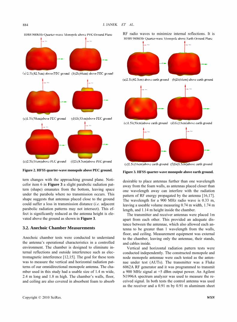
Once these simulations were complete, the PEC ground plane was replaced by an earth-like ground plane. The ground plane was configured with similar dielectric (15) and conductivity (0.008) characteristics of terrain in our WSN field location (see Figure 2(d) from [5]). All antenna simulations were executed varying the antenna height from 0.5λ to 2.5λ in 0.5λ steps. The results of these simulations produced 3-dimensional radiation plots and gain measurements. The radiation plots illustrate an overall shape of the pattern for the antenna as it approa- ched the ground plane.

Figures 2 and 3 are HFSS 3-dimensional radiation plots for a quarter-wave monopole above a PEC ground plane, and a quarter-wave monopole above an earth-like ground plane respectively. The radiation pattern for each height was simulated and illustrate how the vertical pat-

J. JANEK ET AL.


884

Figure 2. HFSS quarter-wave monopole above PEC ground.

tern changes with the approaching ground plane. Noti-cefor item 6 in Figure 3 a slight parabolic radiation pat-tern (shape) emanates from the bottom, leaving space under the parabola where no transmission occurs. This shape suggests that antennas placed close to the ground could suffer a loss in transmission distance (i.e. adjacent parabolic radiation patterns may not intersect). This ef-fect is significantly reduced as the antenna height is ele-vated above the ground as shown in Figure 3. 3.2. Anechoic Chamber Measurements Anechoic chamber tests were conducted to understand the antenna’s operational characteristics in a controlled environment. The chamber is designed to eliminate in-ternal reflections and outside interference such as elec-tromagnetic interference [12,15]. The goal for these tests was to measure the vertical and horizontal radiation pat-terns of our omnidirectional monopole antenna. The chamber used in this study had a usable size of 1.4 m wide, 2.4 m long and 1.8 m high. The chamber’s walls, floor, and ceiling are also covered in absorbent foam to absorb

RF radio waves to minimize internal reflections. It is

Figure 3. HFSS quarter-wave monopole above earth ground.

desirable to place antennas further than one wavelength away from the foam walls, as antennas placed closer than one wavelength away can interfere with the radiation pattern of RF energy propagated by the antenna [16,17]. The wavelength for a 900 MHz radio wave is 0.33 m, leaving a useable volume measuring 0.74 m width, 1.74 m length, and 1.14 m height inside the chamber.

The transmitter and receiver antennas were placed 1m apart from each other. This provided an adequate dis-tance between the antennae, which also allowed each antenna to be greater than 1 wavelength from the walls, floor, and ceiling. Measurement equipment was external to the chamber, leaving only the antennae, their stands, and cables inside.

Vertical and horizontal radiation pattern tests were conducted independently. The constructed monopole and node monopole antennae were each tested as the anten-nae under test (AUTs). The transmitter was a Fluke 6062A RF generator and it was programmed to transmit a 900 MHz signal at +5 dBm output power. An Agilent N1996A spectrum analyzer was used to measure the re-ceived signal. In both tests the control antenna was used as the receiver and a 0.91 m by 0.91 m aluminum sheet

J. JANEK ET AL.


885

was used as a ground plane. In the horizontal radiation test, the control antenna was at a fixed location and height.

The AUT was attached to a device that would rotate the AUT horizontally at fixed intervals of 15˚. This test was repeated with the AUT at vertical heights ranging from 3λ (1 m) down to 0.5λ (16 cm) to measure horizontal radia-tion pattern differences due to the presence of a ground plane. Limitations caused by the combination of test stand mechanics and the physical size of the antenna made measurements at 0.25λ unreliable. The control height was fixed at 3λ (1 m). An example comparison between the anechoic chamber and an HFSS simulation with an anten-na height of 2λ (66 cm) is shown in Figure 4.

Vertical radiation pattern tests required that the AUT be held in a fixed angular position and height. The con-trol antenna was repositioned vertically in 15 degree in-crements about the AUT and kept exactly 1m from the AUT. These tests were also performed with the AUT at vertical heights ranging from 3λ (1 m) down to 0.25λ (8 cm) to measure any affects on the vertical radiation pat-tern due to the presence of a ground plane.

Vertical height limitations of the chamber restricted vertical pattern measurements to less than the full 180˚ desired range. However this does not translate into a problem with the sensor nodes because they were de-signed to be positioned in a horizontal plane, not a ver-tical plane. A larger chamber however would have better enabled more comprehensive data in the vertical plane. It was assumed that maximum power would be received at0◦ horizontal. Received power should decrease as the control antenna’s height was adjusted. The results in Figure 5 appear to be less uniform when compared to the simulated radiation patterns from Figures 2 and 3. Figure 5 does illustrate however that at higher AUT

Figure 4. Horizontal radiation pattern (Anechoic chamber vs. HFSS).

Figure 5. Anechoic chamber vertical pattern results. elevations (82.5 cm and 66 cm) the vertical radiation pattern is significantly more consistent than the lower elevations.

3.3. Field Measurements

The outdoor range test was designed to measure the RF communication distance of two sensor nodes in a real- world environment. The tests were conducted at a uni-versity agriculture research facility located in the midwestern United States.

Three different test fields were studied: bare (not planted or tilled) soil, soybeans, and corn. The tests were conducted in mid-July, so the crops were approaching their full mature size. The same nodes were used for all tests to eliminate variations from one node to another. One node was programmed with a “transmit blink” pro-gram, where it flashed its on-board LED at 1 Hz, and transmitted a communication signal for any receivers to flash their LEDs. The second node was programmed with a “receive blink” program such that when it is in range of the transmitter, the receiver node received a message from the transmitter and responded by flashing its LED. When the receiver was out of range, the signal was lost and the LED stopped flashing.

Tests were performed where the transmitting node height was varied from 2.5λ (82.5 cm) to 0.25λ (8.25 cm) above the ground. Marker flags were setup at increments of 4.1 m, 6.1 m or 3.1 m depending on the crop, up to a total distance of approximately 150 meters. The receiver node was moved to a distance and its minimum height above the ground was measured. In other words, at a set distance the receiver was lowered until it would lose re-ception of the transmitted signal. As the distance away

J. JANEK ET AL.


886

from the transmitter increased, the receiver would nec-essarily need to be higher above the ground in order to receive correctly from the transmitter. This was repeated until the receiver node was at a distance sufficient to require its antenna to be located at least 2.4 m above the ground in order to receive the transmitted signal. This test was repeated for each of the transmitter heights and for the 3 different crop types.

The results of these tests show communication ranges at different antenna heights, whether both antennae are high (2λ lambda and above), both antennas are low (sim-ilar to node-to-node communication), or one is high and one is low (base station-to-node communication).

Figures 6-8 illustrate the communication response in bare soil, soybean, and corn environments respectively. There are several observations that can be made. First there is a clear parabolic transmission effect, meaning that communication occurs in the upper left portion of each graph. For example, examining Figure 6 we see that a transmitter at a height of 0.25λ (8.5 cm and de-noted as 0.25 in the legend) needs a receiver to be mounted at least 100 cm in the air in order to be heard at a distance of 40 m. A receiver that is also at a height of 8.5 cm must be within 15 m to be heard.

Second, the communication performance in a mature corn field was better than expected, meaning the area to the upper left portion of the graph (where communica-tion occurs) is larger than the lower right (where com-munication does not).

4. Communication Range Prediction

The Friis free space equation is useful for calculating the expected free space loss in a system. However, it does not account for earthly and atmospheric losses. Both Golio and Goldsmith presented similar analytical treatments which modify the Friis free space equation with the inclusion of a propagation factor for the presence of the earth (not the atmosphere) by incorporating

Equation (9) into Equation (10).

1 2

42R + R t r

LOS

h hR

d

(11)

Using a Taylor series approximation, Goldsmith mod-ified the phase delay equation:

1 2

42R +R t r

LOS

h hR

d

(12)

This equation is more useful since it incorporates the antenna heights ( th and rh ) into the propagation loss factor. Recall that the results from section III on propagation patterns and losses are also based on antenna height and distance. In section II, the propagation beha-

Figure 6. Required receiver height vs. receiver distance (Bare soil).

Figure 7. Required receiver height vs. receiver distance (Soybeans).

Figure 8. Required receiver height vs. receiver distance (Corn).

vior as the grazing angle approaches 0 (Figure 1) was introduced. A propagation wave that appears to graze the earth’s surface is not absorbed by the earth. As a result, is approximately equal to –1. In addition, when is approximately equal to 0 , RLOS is then approximately equal to 1 2R + R .

During the range testing, the antenna heights ( th and

rh ) were relatively low (< 1 m) and the distance between antennas was much greater , .t rD h h So, 0 ,

1 , 1 2R +RLOSR d , and converted in Equa-tion (12). Equation (11) is now rewritten as (with the Taylor approximation from Equation (12)):

J. JANEK ET AL.


887

2 22

2 2

4

4t r t r t rt r

r t t

G G G G h hh hP P P

d d d

(13)

where rP and tP are in units of dΒm . Converting this in terms of logarithms we have:

10log 20log 40logr t t r t rP P G G h h d (14)

An environmental propagation factor is still missing from Equation (14). If one were to solve for distance, d, with all other parameters known, there would be no way to distinguish if the distance, d, was determined for a particular environment (such as bare soil, corn, or soy-bean). Therefore an “environmental” propagation factor is required to distinguish the communication environ-ment. To determine such a propagation factor, theoretical results from Equation (14) were compared to measured results from our field tests.

First, ,rP the receiver sensitivity, is specified at –98dBm according to the transceiver specifications. It was assumed that during testing the receiver node re-ceived a signal from between –90 to –98 dBm (If the receiver height was lowered, it would lose the signal, indicating a signal magnitude of lower than –98dBm). Because the actual received signal was not measured, the expected receiver sensitivity, exprP , was approximated

to –95 dBm. Second, Equation (14) was used to determine a value

for rP based on the experimental results. For example, using the soil environment with a height th of 82.5 cm,

rG and tG were approximated to be 1.52 (from HFSS simulation results for an ideal monopole), and transmit power was fixed at +5 dBm. Receiver antenna height,

r meash , and distance, dmeasured, data were recorded during the outdoor range tests from section III-C.

5 10log 1.52 1.52

20log 82.5 40log

r meas

measr meas

p d m

h d

(15)

The power difference can now be determined based on expected and measured power

expr diff r r measP P P (16)

This process was repeated for all values of soil with ht = 82.5 cm which gave an array of values for r diffP . The interquartile range was found for the array of values and outliers were eliminated. The average of the remain-ing values in the array was then calculated and the result was placed in a table. This example process resulted in a value representing the propagation factor for soil with the one antenna at 82.5 cm. This method was repeated for the 3 environments (soil, soybeans, corn) and for the 6 different heights of th , (82.5, 66, 50, 33, 16,8), for a total of 18 values. Table 1 shows the 18 propagation

factors, under the assumption of exprP = 95dBm ; tG and rG = 1:52.

Equation (14) was modified to include the new “envi-ronmental” propagation factor, penv. One value is selected from Table 1 based on a corn, soybean, or soil environ-ment and is inserted into the envP value of the modified

Equation (17).

10log 20log

40 log

r t t r t r

env

P P G G h h

d P

(17)

Table 1 and Equation (17) were used to create a series of profiles for the vertical radiation pattern of the trans-mitter antenna. Figure 9 to 11 are illustrations of the data produced by the mathematical model. As the antenna was lowered towards the ground, the parabolic effect na- rrowed and it appeared as if more RF energy was ra-diated in an upward, vertical direction.

There were no obstacles in the soil environment above the ground surface (i.e. no crops) to impede the RF sig-nal strength. As a result, of the 3 crop environments, the soil test promoted the greatest distance with the lowest

Figure 9. Radiation distance vs. antenna height (Soil).

Figure 10. Radiation distance vs. antenna height (Soybean).

Table 1. Environmental propagation values based on theo-retical and measured values.

ht.=82.5(cm)

ht.=66(cm)

ht.=50(cm)

ht.=33(cm)

ht.=16(cm)

ht.=8(cm)

Soil 20.16 19.62 17.67 20.40 17.27 16.33Soybean 24.72 26.16 30.96 27.57 28.67 28.92

Corn 24.20 22.41 23.31 21.54 24.39 22.35

J. JANEK ET AL.


888

Figure 11. Radiation distance vs. antenna height (Corn). receiver heights. With ht at 82.5 cm, 66 cm, and 50 cm, there was virtually no difference in receiver height hr. This indicated that there would be little value in distance gained by increasing the antenna from 50cm to 82.5 cm.

The soybean crop canopy was 45 cm to 55 cm above the surface. As a result, there is little difference between the measured values at antenna heights of 33 cm and 50 cm. When ht was at 82.5 cm and 66 cm, the antenna was fully above the soybean canopy leaving no obstacles. With the antenna at a height of 8 cm, the thick soybean stems and antenna proximity to the ground caused considerable signal attenuation.

Conversely, corn stalks at their base was thinner than the soybeans. In fact, a direct line of sight for was viewed down the corn row for about 30 meters. Across the corn row, the stems were randomly distributed and line of sight was short (about 2 m). Higher up the corn stalks (0.5 m to 2.5 m), the leaves dominate and become thicker, which contributed to more attenuation. Above the leaves, (greater than 2.5 m) the corn stalks were at their thinnest, with few leaves or obstacles. It is assumed that above 2.5 m an RF signal be affected by a minimal amount of attenuation from the corn stalks (measure-ments were not taken above 2.5 m).

To verify the accuracy of the prediction method, a comparison was made between the simulated curves and the measured values. Of the many different plots, the measured values appeared to closely follow the predicted propagation curve. An example of closely related data is shown in Figure 12. It should be pointed out that the presence of the crops did affect the overall curves. For instance, Figure 13 shows the predicted values of corn with a transmitter height, ht, at 16 cm. This places the transmitter basically in air, but as the receiver increases in height, its trajectory is affected by the presence of the leaves.

One noticeable difference between the predicted val-ues and the measured data was that the predicted values created a parabola and thus were only at a value of 0 m

Figure 12. Predicted vs. measured (Soybean, ht = 50 cm)

Figure 13. Predicted vs. measured (Corn, ht = 16 cm). receiver height for a distance of 0m. For all crop envi-ronments, the receiver antenna was at a height of 0 m for at least a few meters, before the receiver antenna had to be raised. This can be seen in Figure 12 for the distance values of –10 m and +10 m; the receiver antenna was still on the ground at minimum height up to 10 meters away from the transmitter, while the predicted value for this distance is approximately 0.11 m for height. Figure 12 Predicted vs. measured (Soybean, th = 50 cm) Figure 13 Predicted vs. measured (Corn, th = 16 cm) 5. Conclusions and Future Work This work sought to develop a better understanding of-sensor node communication performance degradation as a function of antenna proximity to the earth’s surface combined with the effects of obstacles such as typical Midwestern U.S. agricultural crops. Experimental results agreed with the hypothesis that antenna proximity to the ground plays a significant role in limiting the RF range. Test results from simulations, anechoic chamber mea-surements, and field experiments all indicated that as the

J. JANEK ET AL.


889

height of an omnidirectional monopole antenna approa- ched a ground plane, its radiation pattern changed. More specifically, its horizontal propagation shortened, and a parabola-like image of the vertical radiation pattern compressed, suggesting the existence of areas of limited to no horizontal radiation close to the ground. While at-tempts to measure an extended vertical radiation pattern were problematic in the anechoic chamber, our simula-tion results suggest that the vertical radiation pattern in-creases only if the ground plane is a perfect electric con-ductor (which reflects) and not an earth-like ground sur-face (which absorbs).

Field testing confirmed simulation and anechoic chamber test results and motivated the development of an additional loss component, an “environmental” factor, to be incorporated into an existing analytical model of received power rP as a function of transmit power tP , antenna gains tG ; rG , heights ht; hr, and distance d. The environmental factor was developed empirically, by measuring the loss of communication between nodes of variable height in various obstacle conditions including unobstructed (bare soil) conditions, mature soybean, and mature corn fields. Measurement results were then ap-plied as an average of measurements to establish a re-ceived power difference relative to theoretical (expected) values envP . Comparisons made between using the new model and actual field measurements demonstrate that more accurate prediction is possible.

Tests to study the effects of humidity produced more-questions regarding the isolation of variables and so were not reported here. These tests were conducted in the mor- ning and the afternoon, and as such the humidity, tem-perature, and dew point all changed over time as the data were being recorded. Outdoor range testing was accom-plished with the use of a simple software program. The transmitter sent out a signal with instructions that any receiver should “blink” its LED. When the LED stopped blinking, the receiver was deemed out of range. Given that these tests were ultimately for the benefit of a wire-less sensor network, more detailed results may have been possible with a more comprehensive test setup.

Even with these considerations, our model developed to account for the effects of environmental obstacles (crops) on receive power (and therefore propagation dis-tance) demonstrates promise as a useful tool in the dep-loyment of wireless sensor networks whose nodes must be in close proximity to the earth’s surface and where the sensor field contains obstacles in the form of agricultural crops or other plant life. This model can be used by oth-ers to aid in the deployment of similar sensor networks. In the future we plan on developing more granularity in our model, accounting for humidity and the degree of packet loss.

6. Acknowledgements The authors would like to acknowledge the many helpful suggestions of the anonymous reviewers for improving the quality of this paper. 7. References [1] L. Ruiz, T. Barga, F. Silva, H. Assuncao, J. Nogueira,

and A. Loureiro, “On the Design of a Self-Managed Wireless Sensor Network,” Self-Organization in Net-works Today, Vol. 43, No. 8, August 2005, pp. 95-102.

[2] J. J. Evans, J. F. Janek, A. Gum and B. L. Hunter, “Wire-less Sensor Network Design for Flexible Environmental Monitoring,” Journal of Engineering Technology, Vol. 25, No. 1, 2008, pp. 46-52,.

[3] M. Golio, “The RF and Microwave Handbook,” CRC Press LLC, Boca Raton, 2001.

[4] T. Rappaport, “Wireless Communications, Principles and Practice,” Prentice Hall, New Jersey, 1996.

[5] K. Balman and E. Jordan, “Electromagnetic Waves and Radiating Systems,” Prentice Hall, New Jersey, 1968.

[6] C. De-Santis, D. Campbell and F. Schwering, “An Array Technique for Reducing Ground Losses in Teh HF Range,” IEEE Transactions on Antennas and Propaga-tion, Vol. 21, No. 6, November 1973, pp. 769-773.

[7] L. Braten, T. Brevivik and T. Tjelta, “Predicting the At-tenuation Distribution on Line-of-Sight Radio Links due to Melting Snow,” Access Networks, January 2006.

[8] B. Fong, P. Rapajic, G. Hong and A. Fong, “Factors Causing Uncertainties in Outdoor Wireless Wearable Communications,” IEEE Pervsaive Computing, Vol. 2, No. 2, April-June 2003, pp. 16-19.

[9] K. Paran and M. Kamyab, “Electromagnetic Radiation from Vertical Dipole Antennas Near Air-Lossy Soil In-terface: A Finite-Difference Timedomain Simulation,” International Journal of Numerical Modeling: Electronic Networks, Devices and Fields, Vol. 18, No. 2, March 2005, pp. 119-132,.

[10] G. Anastasi, A. Falchi, A. Passarella, M. Conti and E. Gregori, “Performance Measurements of Motes Sensor Networks,” Proceedings of the 7th ACM Symposium on Modeling, Analysis and Simulations of Wireless and Mo-bile Systems (MSWiM04), Lago di Gardi, Italy, October 2004, pp. 174-181.

[11] J. Thelen, D. Goense and K. Langendoen, “Radio Wave Propagation in Potato Fields,” Proceedings from the 1st Workshop on Wireless Network Measurements, Venice, Italy, February 2005.

[12] R. S. Elliot, “Antenna Theory and Design,” John Wiley & Sons, Inc, Hoboken, 1981.

[13] Ansoft Corporation, “Hfss,” April 2007, http://www. ansoft.com/products/hf/hfss.

[14] W. L. Stutzman, “Antenna Theory and Design,” John Wiley & Sons, Inc., Hoboken, 1981.

J. JANEK ET AL.


890

[15] C. Ichelin, J. Ollikainen and P. Vainkainen, “Effects of RF Absorbers on Measurements of Small Antennas in Small Anechoic Chambers,” IEEE Aerospace and Elec-tronic Systems Society, Vol. 16, No. 11, November 2001, pp. 17-20.

[16] J. Appel-Hansen, “Reflectivity Level of Radio Anechoic

Chambers,” IEEE Transactions on Antennas and Propa-gation, Vol. 21, No. 4, July 1973, pp. 490-498.

[17] J. D. Krause, “Antennas,” McGraw-Hill, Inc., New York, 1988.

Documents

Predicting Ground Effects of Omnidirectional Antennas in Wireless