Predicting employee attrition

Predicting employee attrition A study to the predictive power of employee satisfaction on employee attrition

moderated by the geographical location of the employee.

Claire Wijnen

SNR: u1263583

ANR: 611738

Supervisor: Prof. dr. H. J. Brighton

Second reader: Travis J. Wiltshire

Tilburg University

School of Humanities and Digital Science

Tilburg, The Netherlands

May 13th, 2019

1

Preface

Finishing this thesis is part of receiving the master's degree in Data Science and the title MSc.

Before starting this master, I received my bachelor's degree in Organization Science; this

created my interest in companies, how they are organized and perform. First of I want to thank

my supervisor, Henry Brighton, for all the feedback and support during the creation of this

research, and pushing me to use my newly gained knowledge and skills in data analysis. Also,

a huge thanks to my family and friends for giving feedback, going into a discussion, and giving

me other views on this subject which made me perform significantly better.

2

Abstract

Keeping employees satisfied is important for the economic performance of a company and for

retaining the knowledge created by the company. Several reasons are found within the Indian

IT industry why employees leave a company. These reasons will be included as predictor

variables for predicting employee attrition in other geographical location.

The problem stated within this study is how accurate can employee attrition be predicted

based on different employee satisfaction features within different continents. Five prediction

models are tested, and accuracies are compared. Results show that Asia, Europe, and America,

the continents included in this study, are found to have different combinations of employee

satisfaction features for predicting attrition. One of the main findings is that senior management

predicts attritions with the highest accuracy in each continent. However, the accuracy values

could be higher; that is why for future research, the geographical location could be reduced to

regions within a continent to see if the accuracy of predicting attrition increases.

Keywords: employee attrition, employee satisfaction, geographical location, prediction,

machine learning.

3

Content PREFACE ...........................................................................................................................................................1

ABSTRACT .........................................................................................................................................................2

1. INTRODUCTION .......................................................................................................................................5

1.1. PROBLEM STATEMENT AND RESEARCH QUESTION .........................................................................................6

2. RELATED WORK .......................................................................................................................................7

2.1. EMPLOYEE ATTRITION ...........................................................................................................................7 2.2. EMPLOYEE SATISFACTION .......................................................................................................................7 2.3. THE INFLUENCE OF GEOGRAPHICAL LOCATION .............................................................................................9

3. EXPERIMENTAL SETUP ........................................................................................................................... 11

3.1. DESCRIPTION OF THE DATA SOURCE ........................................................................................................ 11 3.2. PRE-PROCESSING ............................................................................................................................... 11

3.2.1. Data transformation ................................................................................................................. 12 3.2.2. Missing values .......................................................................................................................... 13 3.2.3. Dummy variables ...................................................................................................................... 13 3.2.4. Oddities in the data .................................................................................................................. 13

3.3. DATASET DESCRIPTION ........................................................................................................................ 15 3.3.1. Descriptive linear regressions .................................................................................................... 16 3.3.2. Feature overview ...................................................................................................................... 17 3.3.3. Feature importance .................................................................................................................. 17

3.4. ANALYSIS ......................................................................................................................................... 19 3.4.1. Description of the experiments.................................................................................................. 19 3.4.2. Sub-experiments ....................................................................................................................... 20 3.4.3. Evaluation Criteria .................................................................................................................... 21 3.4.4. Algorithms and parameters ...................................................................................................... 22

3.5. SOFTWARE ....................................................................................................................................... 23

4. RESULTS................................................................................................................................................. 24

4.1. EXPERIMENT 1 .................................................................................................................................. 24 4.1.1. Asia .......................................................................................................................................... 24 4.1.2. Europe ...................................................................................................................................... 25 4.1.3. America .................................................................................................................................... 26


4




5. DISCUSSION ........................................................................................................................................... 40

5.1. LIMITATIONS AND FUTURE RESEARCH. ..................................................................................................... 42

6. CONCLUSION ......................................................................................................................................... 43

7. REFERENCES .......................................................................................................................................... 44

8. APPENDIX .............................................................................................................................................. 46

8.1. OBSERVATIONS PER COMPANY .............................................................................................................. 46 8.2. OVERVIEW OF DATASET ....................................................................................................................... 47 8.3. DESCRIPTIVE LINEAR REGRESSIONS ......................................................................................................... 47 8.4. ALGORITHMS AND PARAMETERS EXPLAINED ............................................................................................. 48

8.4.1. Algorithms used in pre-processing............................................................................................. 48 8.4.2. Algorithms used in the experiments .......................................................................................... 48

8.5. COMPARISON OF THE DIFFERENT PARTITION OF THE DATA SET. ...................................................................... 51 8.5.1. Plot comparing models with different partitions of the dataset. ................................................ 51

5

1. Introduction “Truly, the most distinctive feature of our economic system is the growth in

human capital.” (Schultz, 1961, p.1)

Human capital as implied by Schultz (1961) is an essential feature in how an organization is

performing economically. In turn, employees are the keepers of the human capital created by

the company and the employees itself. In a knowledge-driven industry, the main problem has

to do with its key material - the employees (Agarwal, 2015). So, keeping employees satisfied

in their position is of great importance to make sure they do not leave the company and take

their knowledge to another organization. In other words, employee attrition needs to be as low

as possible especially in companies based on knowledge, where the employees are the key

material. Such companies are for example Amazon, Google, Microsoft, and Apple, who

treasure their human capital and so creating an advantage towards their competitors. The

software industry in India is facing the problem of attrition, and it is examining with possible

reasons and has not developed a panacea in attrition control as yet (Agarwal, 2015). Requiring

knowledge about different factors which motivates employees to leave their job, addresses the

issue such as stress, job satisfaction and job commitment, which might have relation and impact

on the attrition of employees (Agarwal, 2015). Much research within this topic has been done

in the information technology (IT) industry of India. Employee satisfaction is viewed as one of

the organizational cultural impacts by which the overall philosophy and attitudes, is the reason

behind how values and dominant goals are established in the organization (Jaksic & Jaksic,

2013). The corporate culture is connected to the location of the employee. Stated by Raina &

Roebuck (2016) is that researchers within the Indian IT industry found multiple reasons for

employee's leaving a company in India. These kinds of reasons are, for example, payment

packages, career level, growth, and relationships with supervisors are cited as the main reasons

for job attrition while others have observed the lack of job security, ease of flexible work

environments, and career advancements are reasons for employees to leave an organization. So,

can the employee satisfaction features found within the software industry in India also be found

in other geographical locations?

6

1.1. Problem statement and research question In this research, the geographical location of the employee will play a big part in measuring

employee satisfaction and employee attrition. Frye, Boomhower, Smith, Vitovsky & Fabricant

(2018) and Agarwal (2015) found that an area for research on this subject is the influence of

location on the prediction of employee satisfaction on employee attrition.

This problem stated in the introduction and by Frye et al. (2015) leads to the following

research question: To what degree can a prediction be made about employee attrition based on

employee satisfaction, and is a difference found between continents? The dataset used for

answering the main research is published on Kaggle.com. The main research question is: How

accurate can employee satisfaction predict employee attrition moderated by the geographical

location of the employee? In particular, this leads to the following question which will provide

an answer for the main research question. These sub-questions are based on the following

employee satisfaction features included in the dataset: work-life balance, culture values, career

opportunities, senior management, and compensation and benefits.

RQ1. How accurately does the work-life balance aspect of employee satisfaction

predict employee attrition within the different continents?

RQ2. How accurately does the culture values aspect of employee satisfaction predict

employee attrition within the different continents?

RQ3. How accurately does the career opportunities aspect of employee satisfaction


RQ4. How accurately does the senior management aspect of employee satisfaction


RQ5. How accurately does the compensations and benefits aspect of employee

satisfaction predict employee attrition within the different continents?

The motivation of this research is that the outcome could be used for establishing advice on

what a trigger point is for employees leaving the company within a specific geographical

location, and how to prevent employees from resigning. It has already been addressed by

Agarwal (2015) that attrition is a problem within the software industry in India. Understanding

what the leading cause is for employees leaving a company is as important as to understand if

there is a geographical reason. With this research, advice will be realized and if this research

can be used as a ruler to what kind of human research (HR) planning needs to be implemented

geographically to keep employees satisfied. So, how to keep a company’s employee attrition as

low as possible at a specific location.

7

2. Related work The dependent variable of this study is employee attrition, synonyms used within scientific

articles are employee turnover, employee quits, employee retention, and employee churn. The

independent variables are employee satisfaction variables, and as moderator, the geographical

location of the employee is added.

2.1. Employee attrition It has already been said in the introduction of this research, that employee turnover has been

identified as a vital issue for organizations. Because when an employee resigns, it brings costs

and loss of knowledge, such as filling up the vacancy, & tolerating a lower skill set from an

underdeveloped replacement (Frye, Boomhower, Smith, Vitovsky, & Fabricant, 2018). This

conclusion is also confirmed by Hoffman & Tadelis (2018); many firms consider turnover to

be a significant problem. High-tech firms are often keenly interested in reducing turnover

because employee knowledge is a crucial asset and turnover is a critical way that knowledge is

lost (Hoffman & Tadelis, 2018). So, gaining an inside in what motivates an employee to resign

is of importance to a company. A possible solution to solve this problem is that organizations

use machine learning techniques to predict employee turnover (Punnoose & Ajit, 2016).

Accurate predictions will enable organizations to take-action for decreasing employee attrition.

(Punnoose & Ajit, 2016). Aside from the reasons named by Punnoose & Ajit (2016), prediction

of the attrition rate is also essential to ensure continuous growth and development of the

business (Khera & Divya, 2019). Recognized is that a single factor does not influence employee

attrition. However, attrition takes place because of several reasons such as employee

satisfaction. Employee satisfaction influences an employee to leave the current work with the

aim to search for better opportunities (Khera & Divya, 2019).

2.2. Employee satisfaction Employee satisfaction is the positive reaction employees have to their overall job

circumstances, including their supervisors, pay and coworkers (Kumar & Pansari, 2015).

Satisfied employees tend to be more committed to their work and have less absenteeism,

connect better with the values and goals of the organization and perceive themselves to be a

part of the organization (Kumar & Pansari, 2015). However, when employees are unsatisfied

by their ineffective working practices, inadequate support of management and inadequate

compensations as well as work-life balance, attrition will take place (Khera & Divya, 2019).

8

The most common reasons for a mismatch between job and worker is that there are no growth

opportunities for the worker, that there is a lack of appreciation from management, and lack of

trust, support, and coordination among co-workers, stress from overload and work-life

imbalance, and not adequately implemented compensation strategies (Sandhya & Kumar,

2011). Employees commonly city their managers' behavior as the primary reason for quitting

their jobs (Reina, Rogers, Peterson, Byron, & & Hom, 2018). As found by several articles is

that managers are central to employee attrition, when managers inspire rather than pressure

their employees, they are better able to retain talent in part because they create an emotional

connection between their employees and their work (Reina, Rogers, Peterson, Byron, & &

Hom, 2018); (Sandhya & Kumar, 2011); (Khera & Divya, 2019).

Another feature of employee satisfaction is compensation and benefits also found to have a

negative impact on attrition, so can act as a critical factor in reducing managerial turnover and

increasing commitment (Das & Baruah, 2013). Also, work-life balance is essential for

employee satisfaction; a healthy balance between the professional and personal life is found to

be stress reducing and not emotional exhausting (Das & Baruah, 2013). This concept can be

defined as an engagement in work and nonwork roles producing an outcome of equal amounts

of satisfaction in work and nonwork life domains (Sirgy & Lee, 2018).

Another feature explained by Das & Baruah (2013) is Promotion and Opportunity for

growth within the company, it is said to be positively correlated with job satisfaction and which

in turn helps in retaining employees, and job flexibility along with lucrative career and life

options is a critical incentive for all employees. The last employee satisfaction feature explained

is the cultural values within a company also known as the work environment. A work

environment that provides a sense of belonging is beneficial for employees, as well generous

human resource policies and providing employees with an appropriate level of privacy and

sound control on work environment (Das & Baruah, 2013). For a company, the task is the

reduce attrition, which means increasing employee satisfaction. However, public managers

tasked with decreasing retention might have better foresight concentrating on their agencies’

unique demographic characteristics and specific management practices, rather than on their

employees’ self-reported aggregated turnover intention (Cohen, Black, & Goodman, 2016).

9

2.3. The influence of geographical location Frye et al. (2018) and Agarwal (2015) found that there is an area for research on the subject of

the influence of location on predicting the employee attrition influenced by employee

satisfaction. Within the study conducted the same companies are observed within a different

location; Thus, could cultural values of different location influence employee attrition?

Moreover, the culture of the different geographical location could vary, which might make the

importance of different feature of employee satisfaction dissimilar.

Culture is shared belief, assumptions, and values held by a group of members, which

influence the attitudes and behaviors of the group members (Raina & Roebuck, 2016). Culture

is measured through different techniques; one of the leading studies in understanding national

culture and norms is Hofstede & Bond (1984). Hofstede & Bond (1984) identified four

dimensions that could influence business cultures: Power distance, uncertainty avoidance,

individualism vs. collectivism, and masculinity vs. femininity.

Power distance is defined as "the extent to which the less powerful members of institutions

and organizations accept that power is distributed unequally" and the underlying societal issue

to which it relates is social inequality and the amount of authority of one person over the others

(Hofstede & Bond, 1984). It could influence how employees see their senior management and

how this could have an impact on employees leaving the organizations. Uncertainty avoidance

is defined as the extent to which people feel threatened by ambiguous situations, and have

created beliefs and institutions that try to avoid these. The societal issue to which it relates is

the way a society deals with conflicts and aggression (Hofstede & Bond, 1984). Individualism

is defined as a situation in which people are supposed to look after themselves and their

immediate family only, whereas its opposite pole, collectivism, is defined as a situation in

which people belong to in-groups or collectivities which are supposed to look after them in

exchange for loyalty (Hofstede & Bond, 1984). Within individualistic cultures, work-family

conflict seems amplified for employees experiencing work/family demands (Sirgy & Lee,

2018). Employees in an individualistic culture are more likely to segregate work and family

roles (Sirgy & Lee, 2018). Masculinity is defined as a situation in which the dominant values

in society are success, money, and things, whereas its opposite pole, femininity, is defined as a

situation in which the dominant values in society are caring for others and the quality life. The

fundamental societal issue to which it relates is the choice of social sex roles and its effects on

people’s self-concepts (Hofstede & Bond, 1984). This dimension can be connected to the

compensations and benefits, a feature of employee satisfaction. Employees within a masculine

company give a more critical influence to getting benefits such as money than within a feminine

10

work environment. Finding a balance within the culture of the workplace and country and

keeping the employee satisfied is of great importance.

When looking at the different continents included in the study, the following culture

descriptions are found based on Hofstede & Bond (1984). When looking at the Hofstede

dimensions; Asia is found to have great importance for power distance, masculinity, and

collectivism. Europe is found to have a culture with a small influence of power distance, based

on individualism and in between masculinity and femininity and very individualistic. America

is found to have a work culture based on being individualistic, with a high uncertainty avoidance

and a considerable power distance, and with a masculine work floor. Grounded, with

discovering that the continents included in this study have different cultures, is that predicting

attrition may change based on employee satisfaction features in each continent, which why this

is investigated within this study. The study will provide an answer to what kind of employee

satisfaction features predict employee attrition and how accurate this prediction is in different

continents.

11

3. Experimental Setup Within this section, the methods are explained on how the data is analyzed and pre-processed.

3.1. Description of the data source In order to answer the research questions in this study, data analysis is performed using a dataset

published on Kaggle.com. The data gathered from Kaggle.com is collected from a publicly

available source named glassdoor.com. Glassdoor.com is a site for finding a job but also for

current or former employees to give a review of the company.

The dataset contains 67529 observations collected over the years from 2008 till 2018, from

different companies, which include Amazon, Facebook, Google, Apple, & Netflix. The

variables which will be used to answer the research question are the location variable, which

shows the geographical location of the employee, the employee satisfaction variables, & the

job title variable, which shows if an employee is a former or current employee. The location

variable which features the geographical location of the employees is used as the moderator.

The following variables will be used to measure employee satisfaction; work-life balance

culture values, career opportunities, compensation and benefits, and senior management, these

variables have each a 5-star rating from 1 to 5 and are used as the independent variable.

The job title variable includes if the employee is a former or current employee to the company;

this variable will be used as the dependent variable to measure attrition. The dataset is not

practical for conducting this study, because of the use of only characters. By creating a dataset

which is functional for conducting analysis, a new dataset is created with the above-reported

variables adapted to useable variables; table 2 shows an overview of the variables used. The

next section will provide an overview of how the original dataset is recoded into a new dataset.

3.2. Pre-processing This step is used for creating a new data set which will be used for answering the research

question and the sub-questions. This section will provide a clear view of how variables will be

transformed into measurable variables, and how the missing values will be treated. The

following section within this study will be performed in RStudio.

12

3.2.1. Data transformation

The data contains 67529 employee reviews, after the data transformation which will include

deleting and imputing values, 39102 employee reviews are left. The location variable from the

employee_reviews dataset will be transformed into a variable which is based on the

classification of the location variable into different continents. The countries featuring in the

dataset will be divided into three different variables as regards in which continent this location

lies. The continents which will be included are Asia (6181 observations), America (29497

observations) & Europe (3424 observations). There is a criterion applied for including

geographical locations; the criterion unholds that there must be more than 30 observation per

location, will it be included in one of the continents studied Asia, Europe or America. Other

location will not be used within this study because of the low observation amount and are

deleted. The new variable will be named Continent and is computed as, Asia = 1, Europe = 2,

and America = 3. The next step is to compute this continent variable into dummy variables.

Three separate binary variables are created, called Asia, Europe, and America, as shown in table

1.

Continent

variable

Geographical location Asia

variable

Europe

variable

America

variable

Asia China, India, Japan, Turkey, Singapore, Israel 1 0 0

Europe Ireland, England, Netherlands, Italy, Germany,

France, Spain, Switzerland, Scotland, Poland,

Russia, Finland

0 1 0

America United States, Canada, Mexico, Costa Rica,

Brazil

0 0 1

Table 1 : Geographical location divided into continents and if the locations are included in the Asia, Europe or America variable.

The variables used for measuring employee satisfaction are the following: work-life balance,

culture values, career opportunities, compensations and benefits, and senior management.

These variables will be computed from character variables to integer variables to make the

variables measurable. Also, the variables are renamed because of the inaccurate current names.

For measuring employee attrition, the following variable, job title, in the data set is used

and computed into a useable variable named Attrition. Job title will be transformed into a binary

value. The value former-employee will have a value of 1 and current-employee will be

13

computed to the value 0. All these transformations are included in a new dataset. This dataset

is used for investigating the relationship between employee satisfaction and employee attrition

moderated by the continents, Asia, Europe, and America. The new dataset will further be

elaborated in section 3.3.

3.2.2. Missing values

Within the new data, there are no missing values found in the attrition variable. However, there

are 32633 observations with missing values in the continent variable and the employee

satisfaction variables. However, the missing values of the continent variables will be removed

because the showing NA’s are location which will not be used in answering the research

questions. These missing values mean that 42.1% is removed from the dataset, 28427

observations based on the continent variable. After removing these observations from the

dataset, there are 39102 observations left in the Data_attrition dataset. However, there are still

some missing values present within the employee satisfaction variables.

Replacing the missing observation from the employee satisfaction variables are done

with imputations; the MICE package in R is used to keep as much information as possible. The

NA’s will be replaced by predictive mean matching, which means that the overall mean of the

variable is replacing the NA’s for each variable. Lastly, the study will be conducted based on

39102 observations.

3.2.3. Dummy variables

Categorical variables need to be represented as numerical variables in multiple regression

methods and are also needed to make a deviation between testing continents, which why

dummy variables are created from the Continent variable. The moderator variable is a

multilevel factor variable with three levels. Each factor level is transformed as a numeric binary

variable. The dummy variables are created through a caret package algorithm named

dummyVars, explained in Appendix 8.4.

3.2.4. Oddities in the data

Oddities are found between different companies. Some of the companies for example Amazon

have a shallow mean score in employee satisfaction compared to Facebook; this could have an

impact on the outcome of this study. Shown in the appendix 8.1. are the companies per continent

and the number of employees per company. These figures show that Amazon is the most

observed company within these continents, whereas Facebook has a low observation number

14

per continent. In figure 3 the mean of the overall rating of employee satisfaction is shown per

company. Shown by these figures is that the most observed company has a low mean rating,

and one of the least observed companies has the highest rating. This observation could influence

the outcome of this study and will be held into regard.

Figure 1: Mean overall rating of employee satisfaction per company.

Another oddity is found with the balance of the attrition variable within the dataset. As shown

in figure 2 is that the dataset gives more current employees (66,7%) than former employees

(33,3%) which means that the dataset is unbalanced. This finding could have an influence on

the results of this study, which why a balance between criteria; sensitivity and specificity will

be evaluated.

Figure 2: Amount of observation divided into current and former employee status.

15

3.3. Dataset Description The new dataset consists of 39102 observations after cleaning and preprocessing the data. Each

of these observations represents one employee based in a company within the branch of online

platforms. Table 2 gives an overview of the variables in the data, and in the appendix under 8.2.

a short view is given on the dataset as it is in RStudio.

Variable Description Type

Dependent

Variable

Attrition Formed by using the characters current and

former to classify into a binary feature, if the

employee is a current employee or former

employee.

Categorical:

2 levels

Independent

Variables

work.life.balance 1 of 5 variables measuring employee

satisfaction.

Numerical:

values 1-5

culture.values 1 of 5 variables measuring employee

satisfaction

Numerical:

values 1-5

career.opp 1 of 5 variables measuring employee

satisfaction

Numerical:

values 1-5

comp.benefit 1 of 5 variables measuring employee

satisfaction

Numerical:

values 1-5

senior.management 1 of 5 variables measuring employee

satisfaction

Numerical:

values 1-5

Moderator Continent Continent represents the geographical

location of the employees divided into

Europa, Asia or America. Where 1 = Asia, 2

= Europe, and 3 = America.

Categorical:

3 levels

Dummy

Variables

Continent.1 This variable is a binary dummy variable and

used as a moderator. Asia represents if an

employee is from Asia (1) or not from Asia

(0). The countries used for creating this

variable are India, Turkey, China, Japan,

Singapore, and Israel.

Numerical:

values 0 and

1

16


used as a moderator. Europe represents if an

employee is from Europe (1) or not from

Europe (0). The countries used for creating

this variable are Russia, Ireland, England,

Netherlands, Germany, Franc, Italy, Spain,

Switzerland, Scotland, Poland, and Finland.

Numerical:

values 0 and

1


used as a moderator. America represents if

an employee is from America (1) or not from

America (0). The countries used for creating

this variable are the United States, Canada,

Mexico, Costa Rica, and Brazil.

Numerical:

values 0 and

1

Table 2: Description of features used in the experiments.

3.3.1. Descriptive linear regressions

Before starting the analysis, descriptive analyses are performed through linear regressions over

the complete dataset after preprocessing, an overview of the linear regressions can be found in

Appendix 8.3.

When performing the linear regressions on the dataset, the following interesting facts are

found, all the employee satisfaction variables when moderated by the continent Asia have a

significant positive effect on attrition. When investigating the same model however now with

Europe as the moderating continent, the following results are found: only the work-life balance

and the compensation and benefits as independent variables have a significant effect. Work-life

balance has a positive effect; compensation and benefits has a negative effect. Furthermore,

investigating the same model but again with another continent as moderator namely America.

The following results are found: only the compensation and benefits has a non-significant

negative effect on attrition whereas the other independent variables have a significant adverse

effect on attrition.

17

3.3.2. Feature overview

Table 2 gives a summary of the features in the dataset. There are two types of features in the

dataset categorical and numerical. The categorical variable, Continent, is rearranged into three

different dummy variables as explained in section 3.2.3. which are numerical. The numerical

features used for measuring employee satisfaction have the values 1 till 5. Where 1 is low

satisfaction and 5 is high satisfaction.

3.3.3. Feature importance

Measuring feature importance is done to perceive if a variable is more important for predicting

attrition. The feature importance is measured by the receiver operating characteristic (ROC)

curve analysis conducted for each attribute with the RF method based on the whole dataset.

ROC curve is the most commonly used way to visualize the performance of a binary classifier.

The importance is shown in figure 3. After discovering the importance of features, checking for

correlation is the next step done. No significant correlations are found between variables, which

means that no variables have to be removed.

Figure 3: Feature selection based on predicting employee attrition

18

19

3.4. Analysis The analysis is performed by using the CARET package within the RStudio. CARET is

explained in Appendix 8.4.

3.4.1. Description of the experiments

How accurate can employee satisfaction features predict employee attrition moderated by the

geographical location? The experiments conducted in this study answers this question.

The goal within each experiment is predicting employee attrition based on one of the

five employee satisfaction variables moderated by three different continents, Asia, Europe, and

America, which are coded into dummy variables. The independent variable, employee

satisfaction, is changing within each experiment. The first experiment is based on work-life

balance aspect of employee satisfaction, experiment 2 is based on culture values aspect of

employee satisfaction, experiment 3 is based on career opportunities aspect of employee

satisfaction, experiment 4 is based on compensation benefits aspect of employee satisfaction,

and experiment 5 is based on the senior management aspect of employee satisfaction.

Each of these experiments is performed by applying the following methods generalized

linear model(glm), random forest (RF), lasso, ridge, and elastic net, these methods are explained

in Appendix 8.4.2. These five methods will be trained on the training set of the data and tested

on the test set. Before each algorithm is trained, the same random seed is set to ensure that each

algorithm uses the same data partitions and repeats. The outcomes of the test set will be

analyzed and compared to see if one of the methods performs better than the other on the test

set. The results will give a clear overview of which method performs best.

To proof that the outcomes of the experiments are valid, repeated cross-validation is

performed within each experiment, with five cross-validation and three repeats. All the

experiments are based on a randomly selected training set of 80% and a test set of 20% of the

dataset; this decision is based on several articles which also use this separation for validating

that models do not overfit, so making reliable prediction (Frye, Boomhower, Smith, Vitovsky,

& Fabricant, 2018); (Khera & Divya, 2019); (Punnoose & Ajit, 2016). Choosing this separation

is also confirmed by testing different separation levels. 50/50, 70/30, and 80/20. Illustrated by

graphs found in appendix 8.5.1. is that 80/20 has the highest accuracy found within all the

models tested.

20

3.4.2. Sub-experiments

How accurately does the work-life balance aspect of employee satisfaction predict employee

attrition within the different continents?

The first experiment addresses RQ1 and is based on the work-life balance variable of employee

satisfaction in the dataset. The goal is investigating how accurate work-life balance can predict

employee attrition moderated by three different continents; Asia, Europe, and America. The

continent variables are dummy variables as explained in part 3.2.3. The independent and

moderator variables are all numeric except for the dependent variable attrition; this is a binary

factor variable. Each of the different continents is tested individually in the models as

moderator. First of Continent.1 is included as a moderator and trained on 80% of the data with

methods glm, random forest, lasso, ridge, and electric net. These models will then be tested on

20 % of the data, which will show the best model. Secondly, the variable Continent.2 is included

as moderator, and Continent.1 is removed. The five different methods are again trained

separately within this model on the data set and tested on the test set, which will give the best

performing model. At last the variable Continent.3 is included as moderator, and Continent.2

is removed from the model, and again the different methods are individually tested. For each

of these tests, a confusion matrix will be created which include the evaluation criteria; these are

explained in section 3.4.2. The accuracy and balance of sensitivity and specificity of each

method will be compared which will be the base of choosing the best model. The same structure

is used when performing the other experiments only with other independent variables, as will

be explained in the following part of this section.

RQ2 is stated as follows: How accurately does the culture values aspect of employee

satisfaction predict employee attrition within the different continents? This research question

is based on the culture values variable of employee satisfaction; this variable will be included

as the independent variable in the interaction. The goal of the second experiment is investigating

how accurate culture values can predict employee attrition moderated by the three different

continents. RQ3 is stated: How accurately does the career opportunities aspect of employee


is based on career opportunities variable of employee satisfaction; this variable is included as

the independent variable in the interaction within this experiment. The goal of the third

experiment is investigating how accurate career opportunities can predict employee attrition

moderated by the three different continents. RQ4 is formulated as follows: How accurately does

the compensation and benefits aspect of employee satisfaction predict employee attrition within

the different continents? This research question will be answered in experiment 4 and is based

21

on the compensation and benefits variable of employee satisfaction; this variable will be

included as the independent variable in the interaction. The goal of this experiment is

investigating how accurate compensation and benefits can predict employee attrition moderated

by Asia, Europe, and America. The last question will be answered in experiment 5. RQ5 is

formulated as follows: How accurately does the senior management aspect of employee


is based on the senior management variable of employee satisfaction; this variable will be

included as the independent variable in the interaction. The goal of the last experiment is

investigating how accurate senior management can predict employee attrition moderated by the

continents included in the study.

These five experiments will be conducted with each including three sub-experiments

arranged by continents. These five experiments will answer the main research question.

3.4.3. Evaluation Criteria

Explained in section 3.4. is that the dataset is randomly partitioned into a training set of 80%

and a test set of 20 %. After partitioning, the model parameters are tuned in every single

experiment and sub-experiments using 5-fold cross-validation repeated three times within the

Classification and Regression Training (CARET) package of R. First these parameters are tuned

on the training set and subsequently tested on the test set. With the confusion matrix algorithm,

the prediction accuracy of the parameters is registered with the following evaluation criteria:

Accuracy, Kappa, NIR, Sensitivity, and Specificity. A confusion matrix includes the elements

as given in table 3. These elements can be found within the different evaluation criteria.

Confusion Matrix reference

0 1

predicted 0 TP FN

1 FP TN

Table 3: Example Confusion Matrix: TN = true negative, TP = true positive,

FP = false positive, & FN = false negative.

22

Accuracy is the proportions of the total number of correct predictions. The accuracy is

calculated as follows: Accuracy = (TP+TN)/(TP+FP+TN+FN) (Gromski, et al.). Proper

measurement of accuracy is 0.8 or higher. However, accuracy alone is not a good enough

measure for an unbalanced dataset, that is why a trade-off between sensitivity and specificity is

also evaluated.

Kappa is a measure of how well the classifier performed as compared to how well it

would have performed merely by chance. In other words, a model will have a high Kappa score

if there is a big difference between the accuracy and the null error rate. The null error rate is

how often someone would be wrong if someone always predicted the majority class (Unknown,

2016).

The no information rate (NIR) is a criterion which indicates the highest value among

the proportion of all positives in the total number of observations which is also known as the

prevalence (Gromski, et al.).

The following formula 𝑆𝑃 = %&%&'()

measures specificity. This calculation is the

number of correct negative predictions (TN) divided by the total number of negatives (TN+FP).

The best specificity is 1.00. Because the positive class is set to reference 1, the specificity is

evaluated (Gromski, et al.). Sensitivity measures the proportion of positive examples that are

correctly classified with the formula SE = %)%)'(&

. The best sensitivity is 1.00. A balance between

sensitivity and specificity is wanted when performing models on the train and test sets of the

data. The outcome of sensitivity and specificity must be close to each other to represent an

excellently balanced prediction for the given models.

After evaluating the models separately, they are compared to investigate the best performing

models for each sub-experiment. The best performing models are used for creating a conclusion

for this research.

3.4.4. Algorithms and parameters

Adjacent the different learning algorithms used in this study are discussed. First, the overall

algorithms are explained which are used by creating the partitioning of the dataset and how the

models are tuned, which are the same for the methods. Generalized linear regression (GLM) is

discussed followed by the learning algorithms; random forest (RF), lasso (LASSO), ridge

(RIDGE), and elastic net (GLMNET). These methods are implemented into the train algorithm

of the caret package which is explained in appendix 8.4.2.

23

3.5. Software The programming language used in this study is RStudio. The RStudio software is used to

download, explore, preprocess the data and perform the experiments. The data file is found on

Kaggle.com under employee_reviews. This data file is downloaded into RStudio. R packages

that are used for pre-processing and data visualization ggplot2, and mice. The experiments are

performed with the following R package; caret.

24

4. Results The results of the experiments conducted are explained in this section; all relevant results will

be summarized within tables. With these results, an overall conclusion may be given to the

main research question. The goal in the first experiment was investigating the predictability of

attrition based on work-life balance with sub-experiments based on the different continents.

The same is done for the second experiment; however, another independent variable is included

culture values videlicet. The third experiment is done with independent variable career

opportunities. The fourth experiment is done with independent variable compensation and

benefits. The last experiment has the same format as the other four experiments but with the

independent variable senior management. Thus, in the next subsections, the results from each

experiment and sub-experiments will be described.

4.1. Experiment 1 As explained in section 3.4.2., experiment 1 is performed with response variables work-life

balance and Continents (Asia, Europe, and America), and predictor variable employee attrition.

Firstly, the best models are chosen per sub-experiment than the results for the sub-experiments

will be explained. Choosing the best models will be done by comparing the accuracy and the

balance of sensitivity and specificity of the models in the test set.

4.1.1. Asia

The first sub-experiment of experiment 1 is done with moderator Asia, predicting employee

attrition based on work-life balance. This experiment is conducted as explained in section 3.4.2.

In order to determine the best model for testing the interaction given in figure 4, a comparison

is made between the five different methods as explained in section 3.4.1. based on the test set

of 20 % of the dataset.

Figure 4: Prediction format work-life balance on employee attrition moderated by Asia.

25

After testing the models on the test set, the results in table 4 show that the best models for

testing work-life balance are RF, GLM, GLMNET, and LASSO with an accuracy of 0.653, and

a Kappa of 0.093. Specificity is also evaluated; the specificity is 0.924 alongside sensitivity

which is found to be 0.153. RIDGE method shows the same accuracy as the no information rate

which why 0 kappa is measured, and the unbalance of sensitivity and specificity. The accuracy

of the other methods is found to be higher than the no information rate of 0.6483 with a better

balance of sensitivity and specificity. The results suggest that the RF, GLM, GLMNET, and

LASSO methods perform the best when predicting attrition based on work-life balance

moderated by Asia.

Methods Accuracy Kappa Specificity Sensitivity

RF 0.653 0.093 0.924 0.153

GLM 0.653 0.093 0.924 0.153

GLMNET 0.653 0.093 0.924 0.153

LASSO 0.653 0.093 0.924 0.153

RIDGE 0.6483 0 1 0

Table 4: The results for predicting attrition by work-life balance moderated by Asia.

4.1.2. Europe

The second sub-experiment of experiment 1 is done with moderator Europe, predicting

employee attrition based on work-life balance. This experiment is conducted as explained in

section 3.4.2. In order to determine the best model for testing the interaction given in figure 5,

a comparison is made between the five different methods explained in section 3.4.1. based on

the test set of 20 % of the dataset.

Figure 5: Prediction format work-life balance on employee attrition moderated by Europe.


testing work-life balance are RF, GLM, and RIDGE, with an accuracy of 0.649, and a Kappa

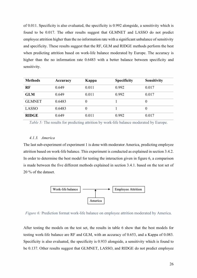
26

of 0.011. Specificity is also evaluated, the specificity is 0.992 alongside, a sensitivity which is

found to be 0.017. The other results suggest that GLMNET and LASSO do not predict

employee attrition higher than the no information rate with a significant unbalance of sensitivity

and specificity. These results suggest that the RF, GLM and RIDGE methods perform the best

when predicting attrition based on work-life balance moderated by Europe. The accuracy is

higher than the no information rate 0.6483 with a better balance between specificity and

sensitivity.


RF 0.649 0.011 0.992 0.017

GLM 0.649 0.011 0.992 0.017

GLMNET 0.6483 0 1 0

LASSO 0.6483 0 1 0

RIDGE 0.649 0.011 0.992 0.017

Table 5: The results for predicting attrition by work-life balance moderated by Europe.

4.1.3. America

The last sub-experiment of experiment 1 is done with moderator America, predicting employee

attrition based on work-life balance. This experiment is conducted as explained in section 3.4.2.


is made between the five different methods explained in section 3.4.1. based on the test set of

20 % of the dataset.

Figure 6: Prediction format work-life balance on employee attrition moderated by America.


testing work-life balance are RF and GLM, with an accuracy of 0.653, and a Kappa of 0.083.

Specificity is also evaluated, the specificity is 0.933 alongside, a sensitivity which is found to

be 0.137. Other results suggest that GLMNET, LASSO, and RIDGE do not predict employee

27

attrition higher than the no information rate with a significant unbalance of sensitivity and

specificity. These results suggest that the RF and GLM methods perform the best when

predicting attrition based on work-life balance moderated by America and the results also show

that the accuracy found is higher than the no information rate 0.6483 with a better balance.


RF 0.653 0.0834 0.933 0.137

GLM 0.653 0.0834 0.933 0.137

GLMNET 0.6483 0 1 0

LASSO 0.6483 0 1 0

RIDGE 0.6483 0 1 0

Table 6: The result for predicting attrition by work-life balance moderated by America.

4.2. Experiment 2 As explained in section 3.4.2., experiment 2 is performed with response variables Culture

Values and Continents (Asia, Europe, and America), and predictor variable employee attrition.

Firstly, the best models are chosen per sub-experiment. Then the results for the sub-experiments

will be explained in the next sub-sections. Choosing the best models will be done by comparing

the accuracy and the balance of sensitivity and specificity.

4.2.1. Asia


attrition based on cultural values. This experiment is conducted as explained in section 3.4.2.




Figure 7: Prediction format culture values on employee attrition moderated by Asia.

28


testing culture values are all the models with an accuracy of 0.653 and a Kappa of 0.0813.

Specificity is 0.936 alongside, a sensitivity which is found to be 0.131. These results suggest

that all the methods can be used for predicting attrition based on culture values moderated by

Asia and the results show that the accuracy found is higher than the no information rate 0.6483.


RF 0.653 0.0813 0.936 0.131

GLM 0.653 0.0813 0.936 0.131

GLMNET 0.653 0.0813 0.936 0.131

LASSO 0.653 0.0813 0.936 0.131

RIDGE 0.653 0.0813 0.936 0.131

Table 7: The results for predicting attrition by culture values moderated by Asia.

4.2.2. Europe


employee attrition based on cultural values. This experiment is conducted as explained in




Figure 8: Prediction format culture values on employee attrition moderated by Europe.


testing culture values are GLM and LASSO, with an accuracy of 0.652, and a Kappa of 0.091.


be 0.154. The accuracy is higher than the no information rate 0.6483. However, the models

chosen to be the best models do not have the highest accuracy; however, the balance between

specificity and sensitivity has better equality as explained in section 3.4.2. The results suggest

29

that the GLM and LASSO methods perform the best when predicting attrition based on culture

values moderated by Europe because of the more balanced results of sensitivity and specificity.


RF 0.653 0.087 0.928 0.144

GLM 0.652 0.091 0.923 0.154

GLMNET 0.653 0.087 0.928 0.144

LASSO 0.652 0.091 0.923 0.154

RIDGE 0.653 0.087 0.928 0.144

Table 8: The results for predicting attrition by culture values moderated by Europe.

4.2.3. America






Figure 9: Prediction format culture on employee attrition moderated by America.


testing culture values are RF, GLMNET, and LASSO, with an accuracy of 0.653, and a Kappa


found to be 0.144. The accuracy found is also higher than the no information rate 0.6483 and

the balance between specificity and sensitivity of the preferred methods is better than the other

methods. Thus, the results suggest that the RF, GLMNET and LASSO methods perform the

best when predicting attrition based on culture values moderated by America.

30


RF 0.653 0.087 0.928 0.144

GLM 0.651 0.07 0.942 0.115

GLMNET 0.653 0.087 0.928 0.144

LASSO 0.653 0.087 0.928 0.144

RIDGE 0.651 0.07 0.942 0.115

Table 9: The results for predicting attrition by culture values moderated by America.

4.3. Experiment 3 As explained in section 3.4.2., experiment 3 is performed with response variables Career

Opportunities and Continents (Asia, Europe, and America), and predictor variable employee

attrition. Firstly, the best models are chosen per sub-experiment. Then the results for the sub-

experiments will be explained in the next sub-sections. Choosing the best models will be done

by comparing the accuracy and the balance of sensitivity and specificity of the models tested

on the test set.

4.3.1. Asia

Sub-experiment 1 of experiment 3 is done with moderator Asia, predicting employee attrition

based on career opportunities. This experiment is conducted as explained in section 3.4.2. In

order to determine the best model for testing the interaction given in figure 10, a comparison is

made between the five different methods as explained in section 3.4.1. based on the test set of


Figure 10: Prediction format career opportunities moderated by Asia.

After testing the models on the test set, the results in table 10 shows that the best models for

testing career opportunities are GLM, LASSO, and RIDGE with an accuracy of 0.651, and a

Kappa of 0.064. Specificity is also evaluated, the specificity is 0.947 alongside, a sensitivity

which is found to be 0.105. The other methods show a higher accuracy of 0.652; however, the

balance is unfavorable compared to the balance of GLM, LASSO, and RIDGE. The accuracy

31

found is higher than the no information rate of 0.6483. These results suggest that the GLM,

LASSO, and RIDGE method performs the best when predicting attrition based on career

opportunities moderated by Asia.


RF 0.652 0.065 0.949 0.104

GLM 0.651 0.064 0.947 0.105

GLMNET 0.652 0.065 0.949 0.104

LASSO 0.651 0.064 0.947 0.105

RIDGE 0.651 0.064 0.947 0.105

Table 10: The results for predicting attrition by career opportunities moderated by Asia.

4.3.2. Europe

Sub-experiment 2 of experiment 3 is done with moderator Europe, predicting employee attrition

based on career opportunities. This experiment is conducted as explained in section 3.4.2. In

order to determine the best model for testing the interaction given in figure 11, a comparison is

made between the five different methods as explained in section 3.4.1. based on the test set of


Figure 11: Prediction format career opportunities moderated by Europe.


testing career opportunities are all the methods. The same accuracies are identified in each of

the models tested, an accuracy of 0.65, and a Kappa of 0.066. Specificity is also evaluated, the

specificity is 0.941 alongside, a sensitivity which is found to be 0.113. These results suggest

that all the method performs the best when predicting attrition based on career opportunities

moderated by Europe. This result is valid because the accuracy is found to be higher than the

no information rate of 0.6483.

32


RF 0.65 0.066 0.941 0.113

GLM 0.65 0.066 0.941 0.113

GLMNET 0.65 0.066 0.941 0.113

LASSO 0.65 0.066 0.941 0.113

RIDGE 0.65 0.066 0.941 0.113

Table 11: The results of predicting attrition by career opportunities moderated by Europe.

4.3.3. America






Figure 12: Prediction format career opportunities moderated by America.


testing career opportunities are GLMNET and LASSO, with an accuracy of 0.65, and a Kappa


found to be 0.113. This balance is also the best within these results. These results suggest that

the GLMNET and LASSO methods perform the best when predicting attrition based on career

opportunities moderated by America and with an accuracy higher than the no information rate

0.6483.


RF 0.649 0.053 0.954 0.089

GLM 0.649 0.052 0.952 0.090

GLMNET 0.65 0.067 0.942 0.113

LASSO 0.65 0.067 0.942 0.113

RIDGE 0.649 0.052 0.952 0.090

Table 12: The results of predicting attrition by career opportunities moderated by America.

33

4.4. Experiment 4 As explained in section 3.4.2., experiment 4 is performed with response variables

Compensation and Benefits, and Continents (Asia, Europe, and America), and predictor

variable employee attrition. Firstly, the best models are chosen per sub-experiment. Then the

results for the sub-experiments will be explained in the next sub-sections. Choosing the best

models will be done by comparing the accuracy and the balance of sensitivity and specificity

of the different models tested on the test set.

4.4.1. Asia

Sub-experiment 1 of experiment 4 is done with moderator Asia, predicting employee attrition

based on compensations and benefits. This experiment is conducted as explained in section

3.4.2. In order to determine the best model for testing the interaction given in figure 13, a

comparison is made between the five different methods explained in section 3.4.1. based on the

test set of 20 % of the dataset.

Figure 13: Prediction format of compensation and benefits moderated by Asia.

After testing the models on the test set, the results in table 13 show that the best model for

testing compensation and benefits is none of the methods. RF results uncover an accuracy of

0.6471 and a Kappa of 0.0182. Specificity is also evaluated, the specificity is 0.979 alongside,

a sensitivity which is found to be 0.036. These results suggest that the RF method performs the

best when predicting attrition based on compensation and benefits moderated by Asia.

However, when compared to the no information rate 0.6483 shows that the accuracy measured

is lower than the no information rate.

34


RF 0.6471 0.0182 0.97870 0.03564

GLM 0.6483 0 1 0

GLMNET 0.6483 0 1 0

LASSO 0.6483 0 1 0

RIDGE 0.6483 0 1 0

Table 13: The results for predicting attrition by compensation and benefits moderated by Asia.

4.4.2. Europe

Sub-experiment 2 of experiment 4 is done with moderator Europe, predicting employee attrition

based on compensations and benefits. This experiment is conducted as explained in section

3.4.2. In order to determine the best model for testing the interaction given in figure 14, a

comparison is made between the five different methods explained in section 3.4.1. based on the

test set of 20 % of the dataset.

Figure 14: Prediction format compensation and benefits moderated by Europe.


testing compensation and benefits is RF, with an accuracy of 0.649, and a Kappa of 0.0046.


be 0.007. The accuracy of the RF method is higher than the no information rate 0.6483, however

it is not the highest accuracy measure. When comparing the balance of specificity and

sensitivity the preferred balance is of RF. These results suggest that the RF method performs

the best when predicting attrition based on compensation and benefits moderated by Europe.

35


RF 0.6485 0.0046 0.996 0.007

GLM 0.6487 0.0048 0.997 0.007

GLMNET 0.6483 0 1 0

LASSO 0.6483 0 1 0

RIDGE 0.6483 0 1 0

Table 14: The results of predicting attrition by compensation and benefits moderated by Europe.

4.4.3. America


attrition based on compensations and benefits. This experiment is conducted as explained in




Figure 15: Prediction format compensation and benefits moderated by America

After testing the models on the test set, the results in table 15 show that the best model found

for testing compensation and benefits is GLM, GLMNET, LASSO, and RIDGE. These models

show an accuracy of 0.6483, which is the same as the no information rate. The balance between

sensitivity and specificity is not preferred whereas the RF model shows a better balance of

sensitivity and specificity. The accuracy of 0.647, and a Kappa of 0.014. These results suggest

that the RF method performs the best when predicting attrition based on compensation and

benefits moderated by America. However, comparing this accuracy of the RF method is not

higher than the no information rate 0.6483. Therefore, none of the models are preferred for

predicting attrition.

36


RF 0.647 0.014 0.982 0.029

GLM 0.6483 0 1 0

GLMNET 0.6483 0 1 0

LASSO 0.6483 0 1 0

RIDGE 0.6483 0 1 0

Table 15: The results of predicting attrition by compensation and benefits moderated by America.

4.5. Experiment 5 As explained in section 3.4.2., experiment 5 is performed with response variables Senior

Management and Continents (Asia, Europe, and America), and predictor variable employee

attrition. Firstly, the best models are chosen per sub-experiment. Then the results for the sub-

experiments will be explained in the next sub-sections. Choosing the best models will be done

by comparing the accuracy and the balance of sensitivity and specificity of the models tested

on the test set.

4.5.1. Asia


attrition based on the senior management aspect of employee satisfaction. This experiment is

conducted as explained in section 3.4.2. In order to determine the best model for testing the

interaction given in figure 16, a comparison is made between the five different methods

explained in section 3.4.1. based on the test set of 20 % of the dataset.

Figure 16: Predicting format senior management moderated by Asia.


testing senior management is RF, with an accuracy of 0.659, and a Kappa of 0.119. The balance

is also evaluated, the specificity is 0.9158 alongside, a sensitivity which is 0.185. The highest

accuracy is found within the other models, but the balance is better within the RF model. The

37

chosen model is the RF model with an accuracy higher than the no information rate. These

results suggest that the RF method performs the best when predicting attrition based on senior

management moderated by Asia.


RF 0.659 0.119 0.91578 0.18545

GLM 0.6593 0.12 0.91637 0.18545

GLMNET 0.6593 0.12 0.91637 0.18545

LASSO 0.6593 0.12 0.91637 0.18545

RIDGE 0.6593 0.12 0.91637 0.18545

Table 16: The results for predicting attrition by senior management moderated by Asia.

4.5.2. Europe


employee attrition based on the senior management aspect of employee satisfaction. This

experiment is conducted as explained in section 3.4.2. In order to determine the best model for

testing the interaction given in figure 17, a comparison is made between the five different

methods explained in section 3.4.1. based on the test set of 20 % of the dataset.

Figure 17: Predicting format senior management moderated by Europe.


testing senior management is RF, with an accuracy of 0.654, and a Kappa of 0.1183. The

balance is also evaluated, the specificity is 0.8982 alongside, a sensitivity which is found to be

0.2036. The balance measured by RF is preferred even as the accuracy which is also higher

than the no information rate. These results suggest that the RF method performs the best when

predicting attrition based on senior management moderated by Europe.

38


RF 0.654 0.1183 0.8982 0.2036

GLM 0.6537 0.1175 0.8982 0.2029

GLMNET 0.6538 0.1178 0.8984 0.2029

LASSO 0.6538 0.1178 0.8984 0.2029

RIDGE 0.651 0.0192 0.9913 0.024

Table 17: The results of predicting attrition by senior management moderated by Europe.

4.5.3. America


attrition based on the senior management aspect of employee satisfaction. This experiment is

conducted as explained in section 3.4.2. In order to determine the best model for testing the

interaction given in figure 18, a comparison is made between the five different methods

explained in section 3.4.1. based on the test set of 20 % of the dataset.

Figure 18: Predicting format senior management moderated by America.


testing senior management are all the models. All the models show the same results as can be

seen in table 18; with an accuracy of 0.657, and a Kappa of 0.103. Specificity is also evaluated,

the specificity is 0.925 alongside, a sensitivity which is found to be 0.162. These results suggest

that all models perform the best when predicting attrition based on senior management

moderated by America, and the accuracies found are higher than the no information rate 0.6483.

39


RF 0.657 0.103 0.925 0.162

GLM 0.657 0.103 0.925 0.162

GLMNET 0.657 0.103 0.925 0.162

LASSO 0.657 0.103 0.925 0.162

RIDGE 0.657 0.103 0.925 0.162

Table 18: The results of predicting attrition by senior management moderated by America.

40

5. Discussion In this section, the study results will be evaluated and discussed. The main findings will be put

against related works, and limitations and recommendations for future research will be stated.

This study was conducted to compare different employee satisfaction aspects and their

prediction factor on employee attrition. Knowing why employees leave the company is vital to

keep the knowledge of the employee within the company. Much research has already been

done, however not with the geographical location added into the interaction. To some extent

has this kind of research already been done. However, in-depth research has only been done in

India. Argwal (2015); Raina & Roebuck (2016), did research within Indian companies. They

stated several reasons why predicting employee attrition is important. These employee attrition

predictors are included within the current study: employee satisfaction aspects included are

work-life balance, culture values, career opportunities, compensation and benefits, and senior

management, which can also be found in the dataset. Will these employee aspects predict

attrition in other countries/continents? Yes, they will, however, these predictors will all have a

different accuracy depending on the continents included.

Work-life balance is essential for employee satisfaction. Within individualistic cultures,

the importance of work-life balance is high as explained by Sirgy & Lee (2018). The continents

found with a high individualistic culture are Europe and America. Expected is that work-life

balance predicts attrition within Europe and America with higher accuracy than in Asia.

However, conflicting results show that Asia (accuracy = 0.653) and America (accuracy = 0.653)

have the highest accuracy, were as Europe (accuracy = 0.649) has an accuracy just higher than

the no information rate. These accuracies result from the RF and GLM models tested for each

sub-experiment. RF shows that the prediction made is non-linear; however, the GLM shows

that the prediction model is linear. An explanation for this observation is that non-linear models

can fit all kinds of curves within the prediction also straight lines whereas linear models cannot

fit these kinds of curves but only straight lines. Because RF and GLM show the same results

concluded is that RF also measures a more linear model.

Culture values on the work floor are also known as the work environment. A work

environment that provides a sense of belonging is beneficial for employees and in keeping the

attrition rate low. The results show that employee attrition in the continents Asia (accuracy =

0.653), Europe (accuracy = 0.652), and America (accuracy = 0.653) can be predicted with a

linear accuracy higher than the no information rate. These results show that cultural values are

41

important in different cultures. Thus, a sense of belonging in the work environment is essential

for many, which why satisfied cultural values are important for predicting attrition.

Opportunities for growth within the company is said to be positively correlated with job

satisfaction, and which in turn helps in keeping attrition low (Das & Baruah, 2013). Found

within the current study, for career opportunity feature of employee satisfaction, is accuracy in

Asia (0.651), Europe (0.65) and America (0.65). These accuracies are just above the no

information rate, but predict employee attrition in each continent with a linear accuracy of 65%.

Compensations and benefits as stated by Das & Baruah (2013), is found to have a

negative impact on attrition, which allows acting as a critical factor in reducing attrition and

increasing commitment. However, found in the study conducted is accuracy not higher or just

higher than the no information rate; Asia (accuracy = 0), Europe (accuracy = 0.6485), and

America (accuracy = 0). Asia and America show a predictive power of 0. However, expected

was that to some degree compensation and benefits predicted attrition. A reason could be that

not the right method has been tested. Moreover, the data was unbalanced; the current employee

group is significantly larger than the former employee group, which could have influenced the

outcome.

Senior management is seen as one of the essential features in predicting employee

satisfaction, as explained in section 2.2. Investigated in this study is, that the highest predictive

power on predicting employee attrition belongs to the aspect of senior management of employee

satisfaction. With the highest measured accuracy of 0.659 and the most balanced sensitivity and

specificity, even though the balance is still not perfect. Senior management is seen as being

able to predict attrition moderated by each continent, with the highest accuracy. A non-linear

prediction model (RF) is found within the continents Asia and Europe whereas America

prediction value fits best with a linear model. This observation may be a consequence of the

unequal amount of observations per continent. America has approximately 30000 observations

considering that Europe and Asia together have just around 10000 observations. When having

a closer amount of observation towards America’s number of observations might create higher

accuracy in linear prediction models. However, the findings are still uniform with the findings

found in scientific literature stating that senior management is the essential feature.

Overall the random forest model performs the best of the models in predicting accuracy.

In total 15 sub-experiments were performed of which 80 % performs best with RF as one of the

methods, 53,3% performs best with GLMNET as one of the methods, 60% with the GLM as

one of the methods, 60% with the LASSO as one of the methods, and 40 % with the RIDGE as

one of the methods. Shown by this is that within several experiments several models were found

42

with the same accuracy. Same accuracies are also found between non-linear versus linear

prediction models. However, explained already is that non-linear could also fit a more linear

prediction whereas linear lines only fit straight lines and not curved lines. This observation

shows that most of the models tested have a linear fit with the predicted interaction.

5.1. Limitations and future research. Some limitations found within the current research are based on performing the analysis and

the data collection. The continent variable is manually constructed by aggregating countries per

continent Asia, Europe or America. The countries within the continents have all different

cultural values, which could mean that they limit each other, when a country gives more value

to one feature of employee satisfaction than another country, within that same continent. This

issue could be the cause of having a low predictive value. Future research could create regions

within the continents with the same company culture to see if the predictive power increases

when adding regions into the prediction of employee attrition.

Another limitation is that the data was not gathered manually, but the whole dataset was

conducted from a site called Kaggle.com. Furthermore, they got the data from a site called

glassdoor.com, the company's, Amazon, Google, Microsoft, Apple, and Netflix, were included

within this dataset. These companies are known for their values and work environment.

Separating the data by different companies could create more accurate prediction within each

continent, which could be done in future research. Because if employees are satisfied or not,

depends on the values and norms of the companies.

Another limitation could be the period in which this data was collected from 2008 till

2018, which is just after the economic crisis. The economic crisis could have made people

easier satisfied with their work than in the second half of the period, where employees had the

freedom of changing jobs. Future research could investigate within this dataset what influence

the economic crisis had on employee attrition.

43

6. Conclusion This study addresses the following problem: How accurate can employee satisfaction predict

employee attrition moderated by the geographical location of the employee? In order to answer

this question, five sub-questions were formulated. Within these five questions, several

predictive models were investigated to see how accurate employee satisfaction factors can

predict employee attrition within different continents. A conclusion can be made based on the

models used is that most of the predictions have a linear fit except for the senior management

feature of employee satisfaction within Asia and Europe.

One of the key findings within this study is that compensation and benefits aspect of employee

satisfaction does not predict employee attrition, this is not a reliable predictor. Employee

satisfaction variables which can be used as a predictor for employee attrition are work-life

balance, cultural values, career opportunities, and senior management. These employee

satisfaction features show accuracy within this study and thus may be used by companies as

predictors. The following key finding is that within each continent another combination of

employee satisfaction features may be used for predicting attrition. Employee attrition can be

predicted in Asia to some accuracy by work-life balance, career opportunities, culture values,

and senior management. Predicting employee attrition within Europe can be done through

cultural values, career opportunities, and senior management. Within America work-life

balance, culture values and senior management factors of employee satisfaction can predict

employee attrition.

Another key finding emerging from this study is that none of the accuracies measured

is higher than 0.8 which is the preferred value for accuracy. All the experiments resulted in

accuracy not higher than 0.66. Still an overall conclusion can be formulated: At least to some

extent; employee satisfaction has predictive power over employee attrition moderated by

continents with an accuracy between 65% and 66%. Concluding is that different combination

of employee satisfaction features can be used by companies to predict employee attrition within

different continents, which allows companies to maintain employee attrition as low as possible

to keep human capital within their company and increasing economic performance.

44

7. References

Agarwal, R. N. (2015). Stress, job satisfaction and job commitment's relation with attrition with

special reference to Indian IT sector. Management and Innovation for Competitive

Advantage.

Bindal, A. (2019, 3 25). Measuring just Accuracy is not enough in machine learning, A better

technique is required.. Retrieved from medium.com:

https://medium.com/datadriveninvestor/measuring-just-accuracy-is-not-enough-in-

machine-learning-a-better-technique-is-required-e7199ac36856

Cohen, G., Black, R. S., & Goodman, D. (2016). Does turnover intention matter? Evaluating

the usefulness of turnover intention rate as a predictor of actual turnover rate. Review of

Public Personnel Administration, 36(3), 240-263.

Das, B. L., & Baruah, M. (2013). Employee retention: A review of literature. Journal of

Business and Management, 14(2), 8 - 16.

Frye, A., Boomhower, C., Smith, M., Vitovsky, L., & Fabricant, S. (2018). Employee Attrition:

What Makes an Employee Quit? SMU Data Science Review, 1, 9.

Gatto, L. (2019, 4 24). An introduction to machine learning with R. Retrieved from Github:

https://lgatto.github.io/IntroMachineLearningWithR/index.html

Gromski, P. S., Correa, E., Vaughan, A. A., Wedge, D. C., Turner, M. L., & Goodacre, R. (n.d.).

A comparison of different chemometrics approaches for the robust classification of

electronic nose data. Analytical and Bioanalytical Chemistry, 406(29), 7581 - 7590.

Hastie, T., & Qian, J. (2014, 06 26). GLMNET vignette. Retrieved from Stanford:

https://web.stanford.edu/~hastie/glmnet/glmnet_alpha.html

Hoffman, M., & Tadelis, S. (2018). People Management Skills, Employee Attrition, and

Manager Rewards: An Empirical Analysis. National Bureau of Economic Research.

Hofstede, G., & Bond, M. H. (1984). Hofstede's culture dimensions: an independent validation

using rokeach's value survey. Journal of Cross-Cultural Psychology, 15(4), 417-433.

Jaksic, M., & Jaksic, M. (2013). Performance Management and Employee Satisfaction.

Montenegrin Journal of Economics, 9, 85.

Khera, S. N., & Divya. (2019). Predictive Modelling of Employee Turnover in the Indian IT

Industry Using Machine Learning Techniques. Vision, 23(1), 12-21.

Kuhn, M. (2019). Package 'caret'. CRAN.

45

Kuhn, M. (2019, 03 27). The caret package. Retrieved from topepo.github.io:

https://topepo.github.io/caret/

Kumar, V., & Pansari, A. (2015). Measuring the Benefits of Employee Engagement. MIT Sloan

Management Review, 56(4), 67 - 72.

Punnoose, R., & Ajit, P. (2016). Prediction of Employee Turnover in Organizations using

Machine Learning Algorithms. International Journal of Advanced Research in

Artificial Intelligence, 5(9), 22 -26.

Raina, R., & Roebuck, D. B. (2016). Exploring Cultural Influence on Managerial

Communication in Relationship to Job Satisfaction, Organizational Commitment, and

the Employees' Propensity to leave in the Insurance sector of India. International

Journal of Business Communication, 53, 97-130.

Reina, C. S., Rogers, K. M., Peterson, S. J., Byron, K., & & Hom, P. W. (2018). Quitting the

boss? The role of manager influence tactics and employee emotional engagement in

voluntary turnover. Journal of leadership & organizational studies, 25(1), 5-18.

Sandhya, K., & Kumar, D. P. (2011). Employee retention by motivation. Indian Journal of

Science and Technology, 4, 1778-1782.

Schultz, T. W. (1961). Investment in Human Capital. The American Economic Review, 51, 1-

17.

Sirgy, J., & Lee, D.-J. (2018). Work-Life Balance: an Integrative Reviw. Applied Research in

Quality of Life, 13(1), 229-254.

Swamy, V. (2018, 10 15). Lasso Versus Ridge Versus Elastic Net. Retrieved from Medium:

https://medium.com/@vijay.swamy1/lasso-versus-ridge-versus-elastic-net-

1d57cfc64b58

Unknown. (2016). Confusion Matrix. Retrieved from Everything about Data Science:

http://scaryscientist.blogspot.com/2016/03/confusion-matrix.html

Van Buuren, S., Groothuis-Oudshoorn, K., Robitzsch, A., Vink, G., Doove, L., Jolani, S., . . .

Gray, B. (2019). Multivariate Imputation by Chained Equations. CRAN.

Wickham, H. (2018). ggplot2 part of the tidyverse. Retrieved from ggplot2.tidyverse.org:

https://ggplot2.tidyverse.org

Yedida, R., Reddy, R., Vahi, R., Jana, R., & Kulkarni, D. (2018). Employee Attrition

Prediction.

46

8. Appendix

8.1. Observations per company

47

8.2. Overview of dataset

8.3. Descriptive linear regressions Moderator = Asia

Independent variable Estimate P-value

Work life balance 0.03964 1.53e-14 *

Culture values 0.032 7.54e-9 *

Career opportunities 0.038 2.22e-11 *

Compensation and benefits 0.025 9.44e-5 *

Senior management 0.039 2.96e-14 *

Moderator = Europe


Work life balance 0.011 0.0864 *

Culture values -0.098 0.1207

Career opportunities -0.0056 0.3912

Compensation and benefits -0.015 0.042 *

Senior management -0.0044 0.474

Moderator = America


Work life balance -0.03 1.33e-12 *

Culture values -0.0133 0.0028 *

Career opportunities -0.01 5.20e-5 *

Compensation and benefits -0.0083 0.119

Senior management -0.0229 6.79e-8 *

ID work.life.balance

culture.values

career.opp

comp. benefit

senior.managem

ent

attrition continent 1 2 3

1 2 3 3 5 3 1 3 0 0 1 2 5 4 5 5 4 0 3 0 0 1 3 2 5 5 4 5 0 3 0 0 1 4 5 5 5 5 5 1 3 0 0 1 5 4 4 4 5 4 1 3 0 0 1

48

8.4. Algorithms and Parameters explained

8.4.1. Algorithms used in pre-processing

The mice package contains functions to inspect the missing data pattern. This algorithm

imputes an incomplete column by generating plausible synthetic values given other columns in

the data (Van Buuren, et al., 2019). The imputations used within this study for the missing

values are the mean values per variable.

The dummyVars algorithm is used for creating dummy variables for one of the

categorical variables with three levels. DummyVars is used for generating a set of dummy

variables from one or more factors. The function takes a formula and a data set and outputs

an object that can be used to create the dummy variables using the predict method (Kuhn,

The caret package, 2019). The created dummy variables are included in the data set and used

in the experiments.

GGPLOT2 is used for creating visualizations of the data as can be seen in figure 1, 2, 3

and appendix 8.1. Ggplot2 is a function with the tidyverse package. Provide the data, tell

ggplot2 how to map variables to aesthetics, what graphical primitives to use, and it takes care

of the details (Wickham, 2018).

8.4.2. Algorithms used in the experiments

Caret is used for the analysis of the data set. Caret package is a package created for RStudio,

which can be used for analyzing datasets through creating training sets, test sets, dummy

variables, doing regressions or other methods and cross-validations, predicting accuracy and

creating confusion matrixes. Caret is a learning algorithm; it is short for Classification and

Regression Training, it contains functions to streamline the model training process for complex

regression and classification problems (Kuhn, The caret package, 2019). The package utilizes

several R packages with different functions that attempt to streamline the model building and

evaluation process, as well as feature selection and other predictive techniques (Kuhn, The caret

package, 2019).

The first step is dividing the data with the function createDataPartition.

CreateDataPartition is used to create balanced splits of the data. The response variable of the

function is a factor; the random sampling occurs within each class and should preserve the

overall class distribution of the data (Kuhn, The caret package, 2019). The split which is

used in the experiments is 80% training data and 20% test data.

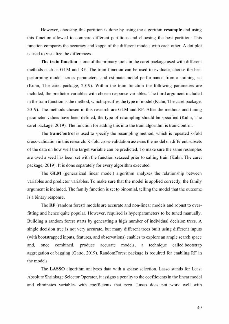
49

However, choosing this partition is done by using the algorithm resample and using

this function allowed to compare different partitions and choosing the best partition. This

function compares the accuracy and kappa of the different models with each other. A dot plot

is used to visualize the differences.

The train function is one of the primary tools in the caret package used with different

methods such as GLM and RF. The train function can be used to evaluate, choose the best

performing model across parameters, and estimate model performance from a training set

(Kuhn, The caret package, 2019). Within the train function the following parameters are

included, the predictor variables with chosen response variables. The third argument included

in the train function is the method, which specifies the type of model (Kuhn, The caret package,

2019). The methods chosen in this research are GLM and RF. After the methods and tuning

parameter values have been defined, the type of resampling should be specified (Kuhn, The

caret package, 2019). The function for adding this into the train algorithm is trainControl.

The trainControl is used to specify the resampling method, which is repeated k-fold

cross-validation in this research. K-fold cross-validation assesses the model on different subsets

of the data on how well the target variable can be predicted. To make sure the same resamples

are used a seed has been set with the function set.seed prior to calling train (Kuhn, The caret

package, 2019). It is done separately for every algorithm executed.

The GLM (generalized linear model) algorithm analyzes the relationship between

variables and predictor variables. To make sure that the model is applied correctly, the family

argument is included. The family function is set to binomial, telling the model that the outcome

is a binary response.

The RF (random forest) models are accurate and non-linear models and robust to over-

fitting and hence quite popular. However, required is hyperparameters to be tuned manually.

Building a random forest starts by generating a high number of individual decision trees. A

single decision tree is not very accurate, but many different trees built using different inputs

(with bootstrapped inputs, features, and observations) enables to explore an ample search space

and, once combined, produce accurate models, a technique called bootstrap

aggregation or bagging (Gatto, 2019). RandomForest package is required for enabling RF in

the models.

The LASSO algorithm analyzes data with a sparse selection. Lasso stands for Least

Absolute Shrinkage Selector Operator, it assigns a penalty to the coefficients in the linear model

and eliminates variables with coefficients that zero. Lasso does not work well with

50

multicollinearity; however found within the data are not high correlations between variables.

Lasso eliminates features, and reduce overfitting in the linear model (Swamy, 2018).

The RIDGE algorithm decreases the complexity of a model but does not reduce the

number of variables to zero or eliminates; it somewhat just shrinks their effect. This algorithm

is also used for measuring linearity and will reduce the impact of features that are not important

in predicting the Y values (Swamy, 2018).

The GLMNET algorithm is a package that fits a generalized linear model via penalized

maximum likelihood. The algorithm is extremely fast and can exploit sparsity in the input

matrix. GLMNET fits linear, logistic and multinomial, poisson, and Cox regression models

(Hastie & Qian, 2014). GLMNET or also known as elastic net combines characteristics of both

lasso and ridge to improve the model's predictions. This algorithm reduces the impact of

different features while not eliminating all of the features (Swamy, 2018).

Predict function is used to understand how accurate the model is at predicting the

response variable. The function takes the model performed and predict the outcomes for the test

dataset.

ConfusionMatrix is applied to check the accuracy by comparing the observed and

predicted results. This function shows a cross-tabulation of the observed and predicted classes.

ConfusionMatrix assumes that the class corresponding to an event is the first level, but it can

be changed by using the positive argument. When performing the confusionMatrix without

changing the positive argument, the level it focusses on is 0; however, it needs to be level 1

which correspond to attrition, so the positive argument is changed to 1. ConfusionMatrix

includes the evaluation criteria of the experiments.

51

8.5. Comparison of the different partition of the data set.

8.5.1. Plot comparing models with different partitions of the dataset.

Figure 18: Comparison between models based on dataset partitions and highest accuracy:

highest accuracy of partition 80/20: 0.6591331 of RF method; Highest accuracy of partition 70/30: 0.6588607 of RF method; Highest accuracy of partition 50/50: 0.6584657 of RF

method

Documents

Predicting employee attrition