Predictable 802.11 Packet Delivery fromWireless Channel Measurements

Daniel Halperin∗, Wenjun Hu∗, Anmol Sheth†, and David Wetherall∗†University of Washington∗ and Intel Labs Seattle†

ABSTRACTRSSI is known to be a fickle indicator of whether a wireless linkwill work, for many reasons. This greatly complicates operationbecause it requires testing and adaptation to find the best rate, trans-mit power or other parameter that is tuned to boost performance.We show that, for the first time, wireless packet delivery can beaccurately predicted for commodity 802.11 NICs from only thechannel measurements that they provide. Our model uses 802.11nChannel State Information measurements as input to an OFDM re-ceiver model we develop by using the concept of effective SNR. Itis simple, easy to deploy, broadly useful, and accurate. It makespacket delivery predictions for 802.11a/g SISO rates and 802.11nMIMO rates, plus choices of transmit power and antennas. We re-port testbed experiments that show narrow transition regions (<2 dBfor most links) similar to the near-ideal case of narrowband, fre-quency-flat channels. Unlike RSSI, this lets us predict the highestrate that will work for a link, trim transmit power, and more. We usetrace-driven simulation to show that our rate prediction is as goodas the best rate adaptation algorithms for 802.11a/g, even over dy-namic channels, and extends this good performance to 802.11n.

Categories and Subject DescriptorsC.2.1 [Computer-Communication Networks]: Network Archi-tecture and Design—Wireless Communication

General TermsDesign, Experimentation

1. INTRODUCTIONWireless LANs based on 802.11 are used almost everywhere,

from airports to zoos and in urban, suburban and rural areas. Mod-ern wireless NICs provide a large and growing range of physicallayer configurations to obtain good performance across this rangeof environments. With 802.11n, the latest version of the standardthat ships on most laptops, combinations of modulation, coding andspatial streams offer rates from 6 Mbps to 600 Mbps [1]. Other im-portant choices include transmit power, channel, and antennas.

For good performance, reliability and coverage, the physical layersettings should match the RF channel over which the wireless sig-nals are sent. This is evident in rate adaptation schemes [5, 10, 14,28] that determine the highest rate for transmission, since a goodscheme has a large effect on throughput. Other work adapts trans-mit power to reduce co-channel interference [17, 21, 25].

Permission to make digital or hard copies of all or part of this work forpersonal or classroom use is granted without fee provided that copies arenot made or distributed for profit or commercial advantage and that copiesbear this notice and the full citation on the first page. To copy otherwise, torepublish, to post on servers or to redistribute to lists, requires prior specificpermission and/or a fee.SIGCOMM’10, August 30–September 3, 2010, New Delhi, India.Copyright 2010 ACM 978-1-4503-0201-2/10/08 ...$10.00.

In theory, it is simple to select the physical layer configurationbecause this is directly determined by the specifics of the RF chan-nel. The signal-to-noise ratio (SNR) is the gold standard for per-formance in narrowband channels. Textbook formulas relate theerror rate of different modulations to the SNR [27]. The best rate orrequired transmit power is then simple to compute.

In practice, 802.11 LANs have never used channel measurementsas more than a coarse indicator of expected performance. Therehave simply been too many ways in which the observed measure-ments and actual performance fail to match the predictions of the-ory. For example, the most accessible channel measurement is re-ceived signal strength indication (RSSI), which serves as a proxyfor the true SNR. RSSI measurements are samples that may varyover packet reception, be mis-calibrated, or be corrupted by in-terference, all of which are known to be issues in practice [6, 10,22]. Even if RSSI were perfect, it does not reflect the frequency-selective fading of 802.11 channels, which are not close to narrow-band. Nor does it account for imperfect receivers that may greatlydegrade performance [3, 10]. Due to these factors, the minimumRSSI at which a rate starts to work varies by more than 10 dB forreal links [22, 30, 31].

To reconcile these viewpoints, a form of guided search is widelyused in practice to select operating points [21, 24, 29]. Packet de-livery is simply tested for a rate or transmit power to see how wellit works. If the loss rate is too high, a lower rate (or more power) isused, otherwise a higher rate (or less power) is tested. SampleRateis a well-known algorithm of this kind for finding transmit rates [5].This approach is very effective for slowly varying channels and sim-ple configurations (e.g., a few rates with fixed transmit power andchannel) since the best setting will soon be found.

However, search becomes less effective as channels change morequickly and the configuration space becomes more complex. Bothof these factors are trends: 802.11 clients are increasingly usedwhen they are truly mobile, both walking and in vehicles; and NICsthat are now being deployed with 802.11n depend on multiple an-tennas, which adds another dimension to and increases the size ofthe search space. Also, tuning combinations such as rate and poweris much more complex.

For rate selection, recent work has made headway by measur-ing symbol-level details of packet reception. In particular, SoftRateuses the output of soft-Viterbi decoding for each symbol to estimatethe bit error rate (BER) [28]. This allows it to predict the effects onpacket delivery of changing the rate. AccuRate uses symbol er-ror vectors for the same purpose [23]. However, these methodsare not defined for selecting other useful parameters, such as trans-mit power, and they do not extend from 802.11a/g to 802.11n, e.g.,when selecting antennas or numbers of spatial streams.

In this work, we return to the basic problem of using theory toconnect the performance of 802.11 NICs on real links to measuredchannels in practice. The opportunity to make progress has arisenfor two reasons. First, 802.11n NICs measure the channel at theOFDM subcarrier level to support MIMO (multiple antenna) op-eration. They report this information in a standard Channel State

1

Information (CSI) format [1]. This provides a much richer sourceof information than RSSI. Note that this CSI naturally applies to802.11a/g rates because they are a subset of 802.11n rates. Sec-ond, modern NICs use OFDM, which gives channel estimates thatare less susceptible to interference than spread spectrum (becauseof lower correlation), and are calibrated. Both factors lead to moremeaningful measurements than in the past.

We use the CSI as input to a model of receiver processing that wedevelop to predict packet delivery. Our model uses the concept ofan effective SNR for a multi-carrier channel [18], such as OFDM,in which there are different subcarrier SNRs, plus approximationsfor coding, interference between MIMO streams, and decoding al-gorithms. It requires no per-link calibration and predicts deliveryfor a wide range of configurations (including rates, transmit power,antenna selection, and spatial streams) from a single CSI measure-ment. We also expect it can be extended to new factors such asbeamforming for even wider applicability in the future.

We make two contributions in this paper. Our main contributionis to show how to accurately predict the performance of commodity802.11 OFDM NICs over real links using only the channel mea-surements that the NIC provides. We believe this to be a first. Ourpacket delivery model is evaluated with measurements over two sta-tionary indoor wireless testbeds built from PCs and 3-antenna In-tel 802.11a/g/n NICs. For a wide range of configurations, we canpredict whether a link will successfully deliver packets (>90%),outside of a narrow (<2 dB for most links) uncertainty region thatis similar to behavior over the near-ideal channel of nodes con-nected by a wire. This lets us consistently predict the best rateto use over a channel, and perform other tasks such as trim ex-cess transmit power. In contrast, RSSI often fails to reflect perfor-mance by a wide enough margin that it does not reliably predictthe best rate or power setting, especially for dense modulation andhigher coding rates (transition >7 dB for 10% of the links). A keyfactor in this improvement is the use of effective SNR to capturefrequency-selective fading, which is clearly visible in our testbeds.No published work has explored effective SNR measures in 802.11beyond simulation, to the best of our knowledge. Note that our ef-fective SNR model does not predict the performance of links underinterference. However, our measurements show that its estimateof interference-free link quality is robust to interfering transmis-sions (§5). We also discuss ways to handle persistent interference.

Our method is practical and can be applied to many classic prob-lems, including rate adaptation, transmit power tuning, and channeland antenna selection. While we must leave most of this to futurework, we demonstrate how our model can inform rate adaptation.Our second contribution is a rate selection algorithm that is as goodas the best 802.11a/g rate adaptation algorithms and extends thisexcellent performance to 802.11n. Our algorithm simply uses ourmodel to predict the highest rate for the channel, repeating to trackthe channel over time. We use a trace-driven simulation to compareit with SampleRate, which is widely used in practice, and SoftRate,which has the best published performance. Our algorithm tracksthe best rate nearly as well as is possible, even for dynamic mobilechannels. It performs very well for MIMO rates, and supports en-hancements such as transmit power trimming and antenna selection.As far as we are aware, there is no other reported work on 802.11nrate adaptation that is evaluated for real, 802.11 channels, and noother rate adaptation algorithms that support these enhancements.

In the rest of this paper, we first motivate the need for better de-livery predictions in §2, and then present our model in §3. Our ex-perimental testbeds are described in §4, and our model is evaluatedin §5. In §6, we use simulation to study rate selection guided byour model. §7 discusses related work, and §8 concludes the paper.

Modulation Coding Rate Data Rate (Mbps)

BPSK 1/2 6.5QPSK 1/2 13.0QPSK 3/4 19.5

QAM-16 1/2 26.0QAM-16 3/4 39.0QAM-64 2/3 52.0QAM-64 3/4 58.5QAM-64 5/6 65.0

Table 1: 802.11n single-stream rates.

2. MOTIVATIONExisting predictions of packet delivery for a given link are based

on its Received Signal Strength Indication (RSSI) value. This iswidely available as a proxy for the SNR. We characterize this map-ping to motivate our research.

802.11 Setting. Our work applies to 802.11a/g/n radios that usecoded Orthogonal Frequency Division Multiplexing (OFDM). 20 or40 MHz channels are divided into 312.5 kHz bands called subcar-riers, each of which sends independent data simultaneously. Con-volutional coding is applied across the bits for error correction andbits are interleaved to spread them in frequency. Each subcarrierin a packet is modulated equally, using BPSK, QPSK, QAM-16, orQAM-64, with 1, 2, 4 or 6 bits per symbol, respectively. The datarates depend on the combination of modulation and coding.

Our experimental platform uses 802.11n radios that operate on20 MHz channels. The single-stream 802.11n rates are shown inTable 1. The main innovation in 802.11n is the use of multiple an-tennas for spatial multiplexing. By using MIMO processing, multi-ple streams can be sent at the same time, each at the single-streamrate, for higher overall rates. Note that the details of single-stream802.11n differ slightly from 802.11a/g (optimized coding rates andmore data subcarriers), but in ways that are not material for ourwork so that we can treat 802.11n as a superset of 802.11a/g.

Packet Delivery versus RSSI/SNR. Textbook analyses of modu-lation schemes give delivery probability for a single signal in termsof the signal-to-noise (SNR) ratio [8], typically expressed on a logscale in decibels. This model holds for narrowband channels withadditive white Gaussian noise. It predicts a sharp transition regionof 1–2 dB over which a link changes from extremely lossy to highlyreliable. This makes the SNR a valuable indicator of performance.

RSSI values reported by NICs give an estimate of the total sig-nal power for each received packet. From RSSI, the packet SNRcan then readily be computed using NIC noise measurements.1 Wegenerated performance curves using SNR for a real 802.11n NICover a simple wired link with a variable attenuator and for a sin-gle transmit and receive antenna. The result is shown for all singleantenna 802.11n rates in Figure 1(a). We observe a characteristicsharp transition region for packet reception rate (PRR) versus SNR.This is despite the relatively wide 20 MHz channel, 56 OFDM sub-carriers, coding and other bit-level operations. This is the behaviorwe want from a link metric in order to predict packet delivery.

In contrast, packet delivery over real wireless channels does notexhibit the same picture. Figure 1(b) shows the measured PRR ver-sus SNR for three sample rates (6.5, 26, and 65 Mbps) over all wire-less links in our testbeds, using the same 802.11n NICs. The SNRof the transition regions can exceed 10 dB, so that some links easilywork for a given SNR and others do not. There is no longer clearseparation between rates. This is consistent with other reported1We refer to the metric computed from RSSI and noise measure-ments as the packet SNR, RSSI-based SNR, or simply RSSI.

2

0 5 10 15 20 25 300

20

40

60

80

100

Packet−level SNR (dB)

PR

R

6.5

13

19.5

26

39

52

58.5

65

(a) A wired 802.11n link with variable attenuation has apredictable relationship between SNR and packet recep-tion rate (PRR) and clear separation between rates.

0 5 10 15 20 25 30 350

20

40

60

80

100

Measured packet SNR (dB)

PR

R

6.5

26

65

(b) Over real wireless channels in our testbeds, the transitionregion varies up to 10 dB. This loses the clear separation be-tween rates (and so only three rates are shown for legibility).

Figure 1: Measured (single antenna) 802.11n packet deliveryover wired and real channels.

measurements that show RSSI does not predict packet delivery forreal links [3, 22, 30, 31].

Impact of Frequency-Selective Fading. Many possible factorscause the observed variability for real channels, including NIC cal-ibration, interference, sampling, and multipath. Here, we look atfrequency-selective fading due to multipath, as our experimentsshow this to be a major factor.

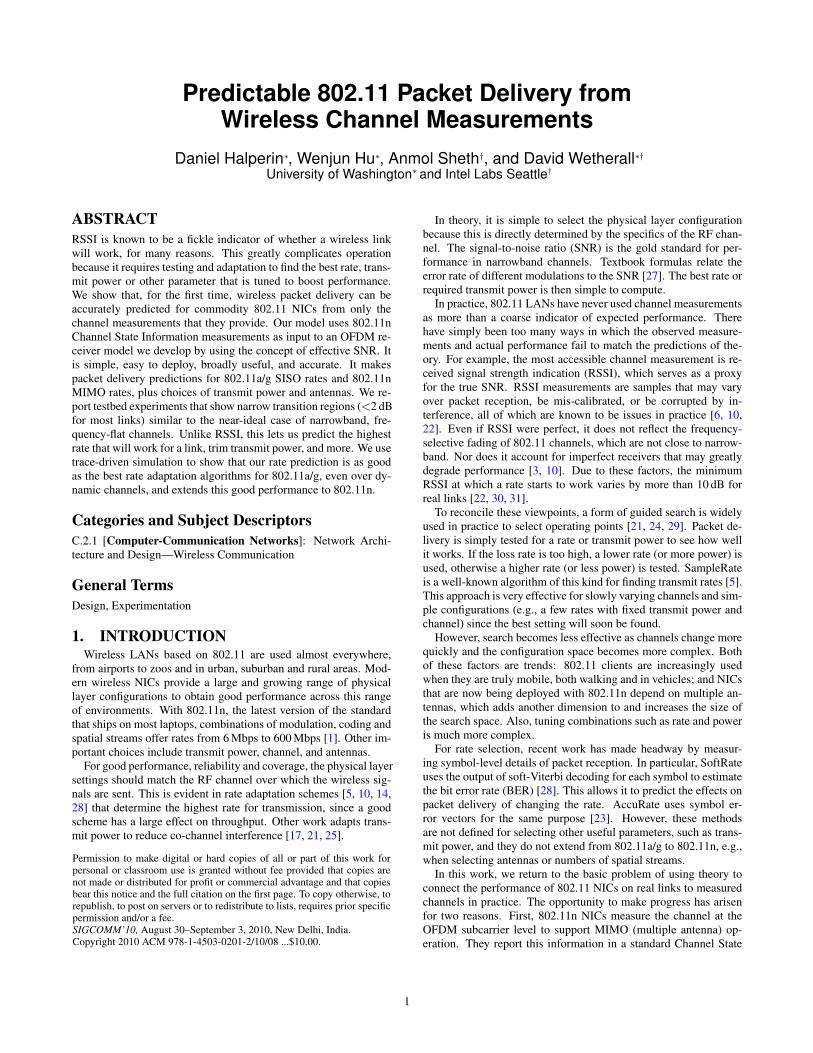
Multipath causes some subcarriers to work markedly better thanothers although all use the same modulation and coding. Thesechannel details, and not simply the overall signal strength as givenby RSSI, affect packet delivery. Figure 2 illustrates this with themeasured subcarrier SNRs for four different links in our testbedaveraged over a 5-second run. All links are shown at the closesttransmit power level, in steps of 2 dB, to 80% packet delivery whenusing the 52 Mbps rate. However, the fading profiles vary signifi-cantly across the four links. One distribution is quite flat across thesubcarriers, while the other three exhibit frequency-selective fadingof varying degrees. Two of the links have two deeply-faded subcar-riers that are more than 20 dB down from the peak.

These links harness the received power with different efficien-cies. The more faded links are more likely to have errors that mustbe repaired with coding, and require extra transmit power to com-pensate. Thus, while the performance is roughly the same, themost frequency-selective link needs a much higher overall packetSNR (30.2 dB) than the frequency-flat link (16.5 dB). This differ-ence of almost 14 dB highlights why RSSI-based SNR does not re-liably predict performance. Fading and its effects are well-known.However, it is rare to see data that shows fading for real links andNICs because it has been difficult to measure.

Impact of multiple streams. The use of multiple antennas adds an-other dimension to the problem of predicting packet delivery. While

5

15

25

35

45

-28 -14 0 14 28

SN

R (

dB

)

Subcarrier index

PRR 83%, SNR 30.2dBPRR 78%, SNR 27.1dBPRR 74%, SNR 18.2dBPRR 80%, SNR 16.5dB

Figure 2: Channel gains on four links that perform aboutequally well at 52 Mbps. The more faded links require largerRSSIs (i.e., more transmit power) to achieve similar PRRs.

we do not present further motivating data here, we briefly note thatthis makes the problem more difficult, not simpler. To begin with,there is now an RSSI for each receive antenna. This makes it dif-ficult to know which RSSI or function of RSSIs to use to predictdelivery even when there is a single spatial stream. When multiplestreams are sent simultaneously, they interfere on the channel. TheMIMO processing used to separate them depends on the details ofthe channel, and less of the signal will be harnessed if the RF pathsare correlated. This adds variability that exacerbates fading effects.

3. PACKET DELIVERY MODELOur goal is to develop a model that can accurately predict the

packet delivery probability of commodity 802.11 NICs for a givenphysical layer configuration operating over a given channel. Wewant our model to be simple and practical, so that it can be readilydeployed, and to cover a wide range of physical layer configura-tions, so that it can be applied in many settings and for many tasks.In particular, the scope of our model is 802.11n including multipleantenna modes, of which single antenna 802.11a/g is a subset. Thisscope is sufficient for many current and future networks. We modeldelivery for single packet transmission only, leaving extensions forinterference and spatial reuse to future work.

Model Design. The structure of our model is simple: given 1) thecurrent state of the RF channel between transmitter and receiver,and 2) a target physical layer configuration of the NIC, it predictswhether that link will reliably deliver packets in that configuration.

For the first piece of input, we use 802.11n Channel State In-formation (CSI). The CSI is a collection of MxN matrices Hs inwhich each describes the RF path (SNR and phase) between allpairs of N transmit and M receive antennas for one subcarrier s.It is reported by the NIC in a format specified by the standard [1],with details in §4.2. An 802.11n NIC can probe a receiver to gatherCSI, or use channel reciprocity to learn CSI from a received packet.The CSI is a much richer source of information than the RSSI, andit gives us the opportunity to develop a much more accurate model.

The second form of input is the target physical layer configura-tion for which we want to predict delivery. This is specified as thechoice of transmit and receive antennas, transmit power level, andtransmit rate (as the combination of modulation, coding, and num-ber of spatial streams). Other choices, such as beamforming, couldbe added in the future. The only restriction is that the CSI includesthe antennas and subcarriers used in the target configuration.

For the model output, we define that the link will work, i.e., willreliably deliver packets, if we predict ≥90% packet reception rate.We do not try to make predictions in the transition region duringwhich a link changes from lossy to reliable. Predictions there are

3

OFDM Demodulator Deinterleaver Convolutional

Decoder Descrambler

(0)Received

signal

MIMO Stream Separation

Separated signalsfor each spatial stream

(1)

Scrambled,coded bits

(3)

(2)Scrambled,interleaved,coded bits

(4)Scrambled bits

(5)Receivedbitstream

Packetprocessing

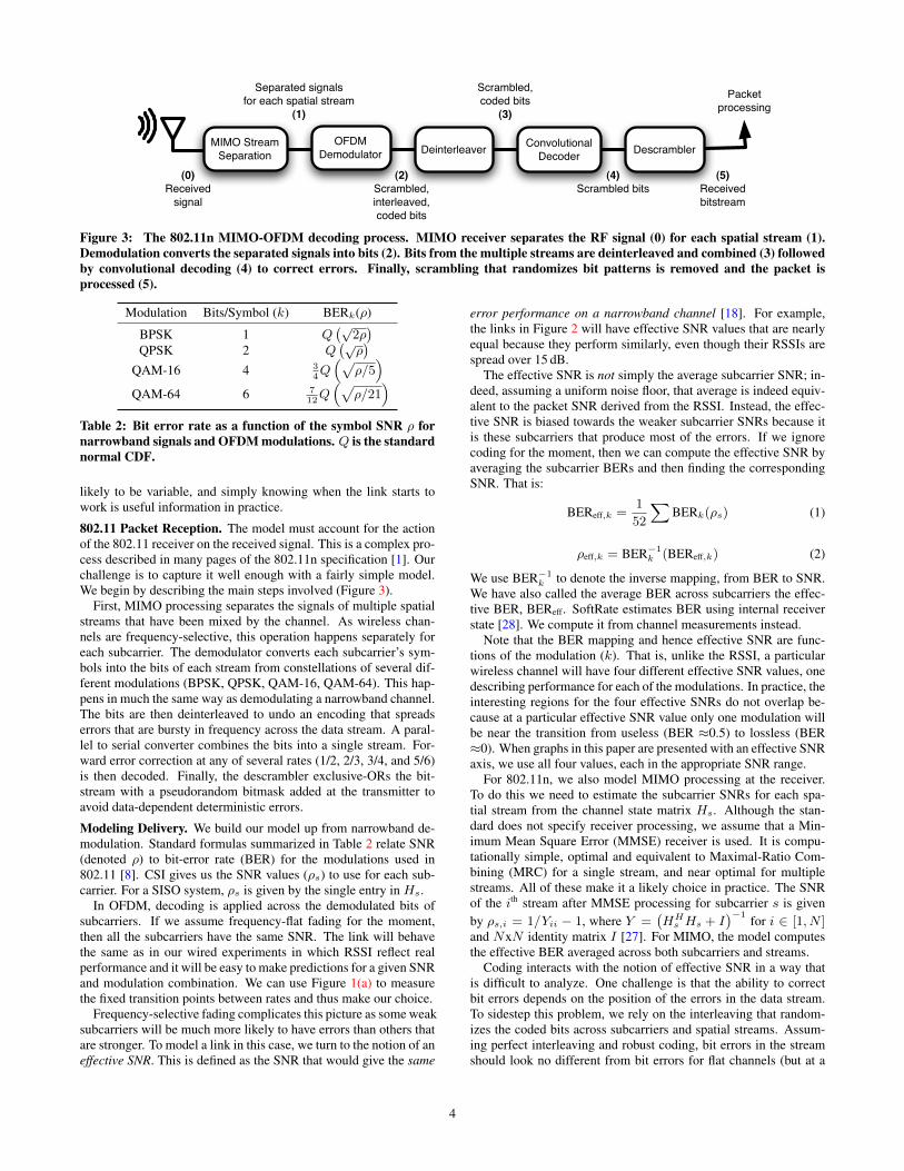
Figure 3: The 802.11n MIMO-OFDM decoding process. MIMO receiver separates the RF signal (0) for each spatial stream (1).Demodulation converts the separated signals into bits (2). Bits from the multiple streams are deinterleaved and combined (3) followedby convolutional decoding (4) to correct errors. Finally, scrambling that randomizes bit patterns is removed and the packet isprocessed (5).

Modulation Bits/Symbol (k) BERk(ρ)

BPSK 1 Q(√

2ρ)

QPSK 2 Q(√ρ)

QAM-16 4 34Q(√

ρ/5)

QAM-64 6 712Q(√

ρ/21)

Table 2: Bit error rate as a function of the symbol SNR ρ fornarrowband signals and OFDM modulations. Q is the standardnormal CDF.

likely to be variable, and simply knowing when the link starts towork is useful information in practice.

802.11 Packet Reception. The model must account for the actionof the 802.11 receiver on the received signal. This is a complex pro-cess described in many pages of the 802.11n specification [1]. Ourchallenge is to capture it well enough with a fairly simple model.We begin by describing the main steps involved (Figure 3).

First, MIMO processing separates the signals of multiple spatialstreams that have been mixed by the channel. As wireless chan-nels are frequency-selective, this operation happens separately foreach subcarrier. The demodulator converts each subcarrier’s sym-bols into the bits of each stream from constellations of several dif-ferent modulations (BPSK, QPSK, QAM-16, QAM-64). This hap-pens in much the same way as demodulating a narrowband channel.The bits are then deinterleaved to undo an encoding that spreadserrors that are bursty in frequency across the data stream. A paral-lel to serial converter combines the bits into a single stream. For-ward error correction at any of several rates (1/2, 2/3, 3/4, and 5/6)is then decoded. Finally, the descrambler exclusive-ORs the bit-stream with a pseudorandom bitmask added at the transmitter toavoid data-dependent deterministic errors.

Modeling Delivery. We build our model up from narrowband de-modulation. Standard formulas summarized in Table 2 relate SNR(denoted ρ) to bit-error rate (BER) for the modulations used in802.11 [8]. CSI gives us the SNR values (ρs) to use for each sub-carrier. For a SISO system, ρs is given by the single entry in Hs.

In OFDM, decoding is applied across the demodulated bits ofsubcarriers. If we assume frequency-flat fading for the moment,then all the subcarriers have the same SNR. The link will behavethe same as in our wired experiments in which RSSI reflect realperformance and it will be easy to make predictions for a given SNRand modulation combination. We can use Figure 1(a) to measurethe fixed transition points between rates and thus make our choice.

Frequency-selective fading complicates this picture as some weaksubcarriers will be much more likely to have errors than others thatare stronger. To model a link in this case, we turn to the notion of aneffective SNR. This is defined as the SNR that would give the same

error performance on a narrowband channel [18]. For example,the links in Figure 2 will have effective SNR values that are nearlyequal because they perform similarly, even though their RSSIs arespread over 15 dB.

The effective SNR is not simply the average subcarrier SNR; in-deed, assuming a uniform noise floor, that average is indeed equiv-alent to the packet SNR derived from the RSSI. Instead, the effec-tive SNR is biased towards the weaker subcarrier SNRs because itis these subcarriers that produce most of the errors. If we ignorecoding for the moment, then we can compute the effective SNR byaveraging the subcarrier BERs and then finding the correspondingSNR. That is:

BEReff,k =1

52

∑BERk(ρs) (1)

ρeff,k = BER−1k (BEReff,k) (2)

We use BER−1k to denote the inverse mapping, from BER to SNR.

We have also called the average BER across subcarriers the effec-tive BER, BEReff. SoftRate estimates BER using internal receiverstate [28]. We compute it from channel measurements instead.

Note that the BER mapping and hence effective SNR are func-tions of the modulation (k). That is, unlike the RSSI, a particularwireless channel will have four different effective SNR values, onedescribing performance for each of the modulations. In practice, theinteresting regions for the four effective SNRs do not overlap be-cause at a particular effective SNR value only one modulation willbe near the transition from useless (BER ≈0.5) to lossless (BER≈0). When graphs in this paper are presented with an effective SNRaxis, we use all four values, each in the appropriate SNR range.

For 802.11n, we also model MIMO processing at the receiver.To do this we need to estimate the subcarrier SNRs for each spa-tial stream from the channel state matrix Hs. Although the stan-dard does not specify receiver processing, we assume that a Min-imum Mean Square Error (MMSE) receiver is used. It is compu-tationally simple, optimal and equivalent to Maximal-Ratio Com-bining (MRC) for a single stream, and near optimal for multiplestreams. All of these make it a likely choice in practice. The SNRof the ith stream after MMSE processing for subcarrier s is givenby ρs,i = 1/Yii − 1, where Y =

(HH

s Hs + I)−1

for i ∈ [1, N ]and NxN identity matrix I [27]. For MIMO, the model computesthe effective BER averaged across both subcarriers and streams.

Coding interacts with the notion of effective SNR in a way thatis difficult to analyze. One challenge is that the ability to correctbit errors depends on the position of the errors in the data stream.To sidestep this problem, we rely on the interleaving that random-izes the coded bits across subcarriers and spatial streams. Assum-ing perfect interleaving and robust coding, bit errors in the streamshould look no different from bit errors for flat channels (but at a

4

50 ft

������

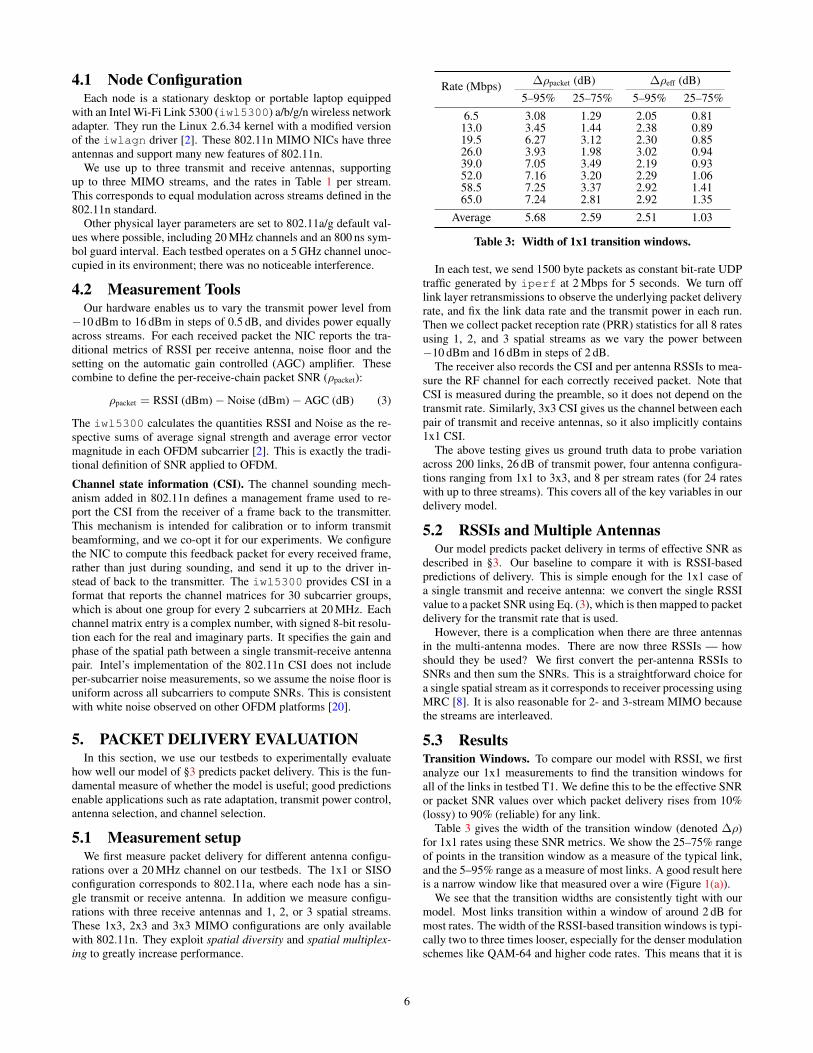
Figure 4: Our indoor 802.11n testbeds, T1 and T2. T1 consists of 10 nodes spread over 8 100 square feet, and T2 consists of 11 nodesspread over 20 000 square feet. The nodes are placed to ensure a large number of links between them, a variety of distance betweennodes, and diverse scattering characteristics.

8

12

16

20

24

-28 -14 0 14 28

SN

R (

dB

)

Subcarrier index

BPSK

QPSK

QAM-16

QAM-64

Packet SNR

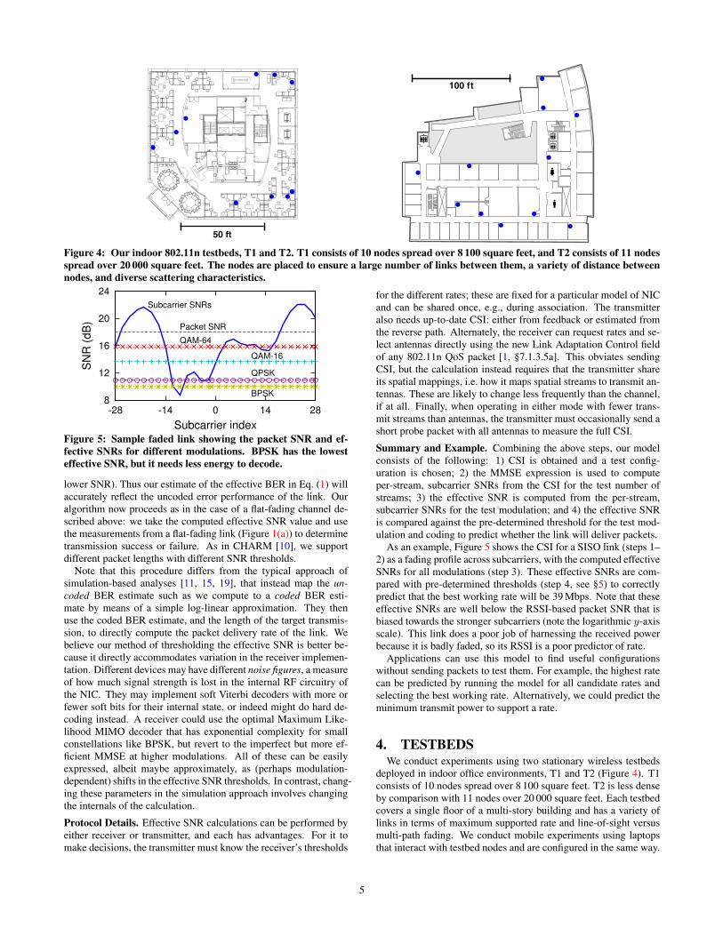
Subcarrier SNRs

Figure 5: Sample faded link showing the packet SNR and ef-fective SNRs for different modulations. BPSK has the lowesteffective SNR, but it needs less energy to decode.

lower SNR). Thus our estimate of the effective BER in Eq. (1) willaccurately reflect the uncoded error performance of the link. Ouralgorithm now proceeds as in the case of a flat-fading channel de-scribed above: we take the computed effective SNR value and usethe measurements from a flat-fading link (Figure 1(a)) to determinetransmission success or failure. As in CHARM [10], we supportdifferent packet lengths with different SNR thresholds.

Note that this procedure differs from the typical approach ofsimulation-based analyses [11, 15, 19], that instead map the un-coded BER estimate such as we compute to a coded BER esti-mate by means of a simple log-linear approximation. They thenuse the coded BER estimate, and the length of the target transmis-sion, to directly compute the packet delivery rate of the link. Webelieve our method of thresholding the effective SNR is better be-cause it directly accommodates variation in the receiver implemen-tation. Different devices may have different noise figures, a measureof how much signal strength is lost in the internal RF circuitry ofthe NIC. They may implement soft Viterbi decoders with more orfewer soft bits for their internal state, or indeed might do hard de-coding instead. A receiver could use the optimal Maximum Like-lihood MIMO decoder that has exponential complexity for smallconstellations like BPSK, but revert to the imperfect but more ef-ficient MMSE at higher modulations. All of these can be easilyexpressed, albeit maybe approximately, as (perhaps modulation-dependent) shifts in the effective SNR thresholds. In contrast, chang-ing these parameters in the simulation approach involves changingthe internals of the calculation.

Protocol Details. Effective SNR calculations can be performed byeither receiver or transmitter, and each has advantages. For it tomake decisions, the transmitter must know the receiver’s thresholds

for the different rates; these are fixed for a particular model of NICand can be shared once, e.g., during association. The transmitteralso needs up-to-date CSI: either from feedback or estimated fromthe reverse path. Alternately, the receiver can request rates and se-lect antennas directly using the new Link Adaptation Control fieldof any 802.11n QoS packet [1, §7.1.3.5a]. This obviates sendingCSI, but the calculation instead requires that the transmitter shareits spatial mappings, i.e. how it maps spatial streams to transmit an-tennas. These are likely to change less frequently than the channel,if at all. Finally, when operating in either mode with fewer trans-mit streams than antennas, the transmitter must occasionally send ashort probe packet with all antennas to measure the full CSI.

Summary and Example. Combining the above steps, our modelconsists of the following: 1) CSI is obtained and a test config-uration is chosen; 2) the MMSE expression is used to computeper-stream, subcarrier SNRs from the CSI for the test number ofstreams; 3) the effective SNR is computed from the per-stream,subcarrier SNRs for the test modulation; and 4) the effective SNRis compared against the pre-determined threshold for the test mod-ulation and coding to predict whether the link will deliver packets.

As an example, Figure 5 shows the CSI for a SISO link (steps 1–2) as a fading profile across subcarriers, with the computed effectiveSNRs for all modulations (step 3). These effective SNRs are com-pared with pre-determined thresholds (step 4, see §5) to correctlypredict that the best working rate will be 39 Mbps. Note that theseeffective SNRs are well below the RSSI-based packet SNR that isbiased towards the stronger subcarriers (note the logarithmic y-axisscale). This link does a poor job of harnessing the received powerbecause it is badly faded, so its RSSI is a poor predictor of rate.

Applications can use this model to find useful configurationswithout sending packets to test them. For example, the highest ratecan be predicted by running the model for all candidate rates andselecting the best working rate. Alternatively, we could predict theminimum transmit power to support a rate.

4. TESTBEDSWe conduct experiments using two stationary wireless testbeds

deployed in indoor office environments, T1 and T2 (Figure 4). T1consists of 10 nodes spread over 8 100 square feet. T2 is less denseby comparison with 11 nodes over 20 000 square feet. Each testbedcovers a single floor of a multi-story building and has a variety oflinks in terms of maximum supported rate and line-of-sight versusmulti-path fading. We conduct mobile experiments using laptopsthat interact with testbed nodes and are configured in the same way.

5

4.1 Node ConfigurationEach node is a stationary desktop or portable laptop equipped

with an Intel Wi-Fi Link 5300 (iwl5300) a/b/g/n wireless networkadapter. They run the Linux 2.6.34 kernel with a modified versionof the iwlagn driver [2]. These 802.11n MIMO NICs have threeantennas and support many new features of 802.11n.

We use up to three transmit and receive antennas, supportingup to three MIMO streams, and the rates in Table 1 per stream.This corresponds to equal modulation across streams defined in the802.11n standard.

Other physical layer parameters are set to 802.11a/g default val-ues where possible, including 20 MHz channels and an 800 ns sym-bol guard interval. Each testbed operates on a 5 GHz channel unoc-cupied in its environment; there was no noticeable interference.

4.2 Measurement ToolsOur hardware enables us to vary the transmit power level from−10 dBm to 16 dBm in steps of 0.5 dB, and divides power equallyacross streams. For each received packet the NIC reports the tra-ditional metrics of RSSI per receive antenna, noise floor and thesetting on the automatic gain controlled (AGC) amplifier. Thesecombine to define the per-receive-chain packet SNR (ρpacket):

ρpacket = RSSI (dBm)− Noise (dBm)− AGC (dB) (3)

The iwl5300 calculates the quantities RSSI and Noise as the re-spective sums of average signal strength and average error vectormagnitude in each OFDM subcarrier [2]. This is exactly the tradi-tional definition of SNR applied to OFDM.

Channel state information (CSI). The channel sounding mech-anism added in 802.11n defines a management frame used to re-port the CSI from the receiver of a frame back to the transmitter.This mechanism is intended for calibration or to inform transmitbeamforming, and we co-opt it for our experiments. We configurethe NIC to compute this feedback packet for every received frame,rather than just during sounding, and send it up to the driver in-stead of back to the transmitter. The iwl5300 provides CSI in aformat that reports the channel matrices for 30 subcarrier groups,which is about one group for every 2 subcarriers at 20 MHz. Eachchannel matrix entry is a complex number, with signed 8-bit resolu-tion each for the real and imaginary parts. It specifies the gain andphase of the spatial path between a single transmit-receive antennapair. Intel’s implementation of the 802.11n CSI does not includeper-subcarrier noise measurements, so we assume the noise floor isuniform across all subcarriers to compute SNRs. This is consistentwith white noise observed on other OFDM platforms [20].

5. PACKET DELIVERY EVALUATIONIn this section, we use our testbeds to experimentally evaluate

how well our model of §3 predicts packet delivery. This is the fun-damental measure of whether the model is useful; good predictionsenable applications such as rate adaptation, transmit power control,antenna selection, and channel selection.

5.1 Measurement setupWe first measure packet delivery for different antenna configu-

rations over a 20 MHz channel on our testbeds. The 1x1 or SISOconfiguration corresponds to 802.11a, where each node has a sin-gle transmit or receive antenna. In addition we measure configu-rations with three receive antennas and 1, 2, or 3 spatial streams.These 1x3, 2x3 and 3x3 MIMO configurations are only availablewith 802.11n. They exploit spatial diversity and spatial multiplex-ing to greatly increase performance.

Rate (Mbps) ∆ρpacket (dB) ∆ρeff (dB)5–95% 25–75% 5–95% 25–75%

6.5 3.08 1.29 2.05 0.8113.0 3.45 1.44 2.38 0.8919.5 6.27 3.12 2.30 0.8526.0 3.93 1.98 3.02 0.9439.0 7.05 3.49 2.19 0.9352.0 7.16 3.20 2.29 1.0658.5 7.25 3.37 2.92 1.4165.0 7.24 2.81 2.92 1.35

Average 5.68 2.59 2.51 1.03

Table 3: Width of 1x1 transition windows.

In each test, we send 1500 byte packets as constant bit-rate UDPtraffic generated by iperf at 2 Mbps for 5 seconds. We turn offlink layer retransmissions to observe the underlying packet deliveryrate, and fix the link data rate and the transmit power in each run.Then we collect packet reception rate (PRR) statistics for all 8 ratesusing 1, 2, and 3 spatial streams as we vary the power between−10 dBm and 16 dBm in steps of 2 dB.

The receiver also records the CSI and per antenna RSSIs to mea-sure the RF channel for each correctly received packet. Note thatCSI is measured during the preamble, so it does not depend on thetransmit rate. Similarly, 3x3 CSI gives us the channel between eachpair of transmit and receive antennas, so it also implicitly contains1x1 CSI.

The above testing gives us ground truth data to probe variationacross 200 links, 26 dB of transmit power, four antenna configura-tions ranging from 1x1 to 3x3, and 8 per stream rates (for 24 rateswith up to three streams). This covers all of the key variables in ourdelivery model.

5.2 RSSIs and Multiple AntennasOur model predicts packet delivery in terms of effective SNR as

described in §3. Our baseline to compare it with is RSSI-basedpredictions of delivery. This is simple enough for the 1x1 case ofa single transmit and receive antenna: we convert the single RSSIvalue to a packet SNR using Eq. (3), which is then mapped to packetdelivery for the transmit rate that is used.

However, there is a complication when there are three antennasin the multi-antenna modes. There are now three RSSIs — howshould they be used? We first convert the per-antenna RSSIs toSNRs and then sum the SNRs. This is a straightforward choice fora single spatial stream as it corresponds to receiver processing usingMRC [8]. It is also reasonable for 2- and 3-stream MIMO becausethe streams are interleaved.

5.3 ResultsTransition Windows. To compare our model with RSSI, we firstanalyze our 1x1 measurements to find the transition windows forall of the links in testbed T1. We define this to be the effective SNRor packet SNR values over which packet delivery rises from 10%(lossy) to 90% (reliable) for any link.

Table 3 gives the width of the transition window (denoted ∆ρ)for 1x1 rates using these SNR metrics. We show the 25–75% rangeof points in the transition window as a measure of the typical link,and the 5–95% range as a measure of most links. A good result hereis a narrow window like that measured over a wire (Figure 1(a)).

We see that the transition widths are consistently tight with ourmodel. Most links transition within a window of around 2 dB formost rates. The width of the RSSI-based transition windows is typi-cally two to three times looser, especially for the denser modulationschemes like QAM-64 and higher code rates. This means that it is

6

0

13

26

52

650

13

26

52

65

0 10 20 30 40 50

Rate

(M

bps)

SNR (dB)

Pkt SNR, best linkPkt SNR, worst link

Eff SNR, best linkEff SNR, worst link

(a) Single spatial stream, single receive antenna (1x1)

0

13

26

52

650

13

26

52

65

0 10 20 30 40 50

Rate

(M

bps)

SNR (dB)

Pkt SNR, best linkPkt SNR, worst link

Eff SNR, best linkEff SNR, worst link

(b) Single spatial stream, three receive antennas (1x3)

0

13

26

52

650

13

26

52

65

0 10 20 30 40 50

Rate

/ s

tream

(M

bps)

SNR (dB)

Pkt SNR, best linkPkt SNR, worst link

Eff SNR, best linkEff SNR, worst link

(c) Two spatial streams, three receive antennas (2x3)

0

13

26

52

650

13

26

52

65

0 10 20 30 40 50

Rate

/ s

tream

(M

bps)

SNR (dB)

Pkt SNR, best linkPkt SNR, worst link

Eff SNR, best linkEff SNR, worst link

(d) Three spatial streams, three receive antennas (3x3)

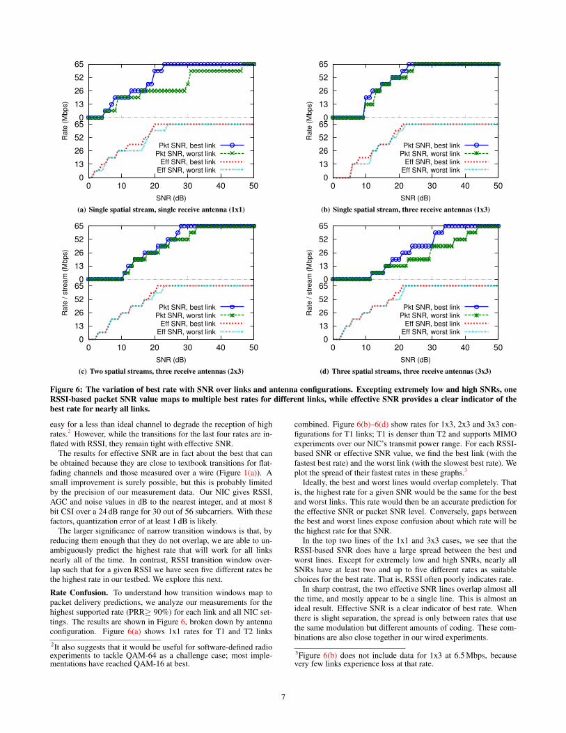
Figure 6: The variation of best rate with SNR over links and antenna configurations. Excepting extremely low and high SNRs, oneRSSI-based packet SNR value maps to multiple best rates for different links, while effective SNR provides a clear indicator of thebest rate for nearly all links.

easy for a less than ideal channel to degrade the reception of highrates.2 However, while the transitions for the last four rates are in-flated with RSSI, they remain tight with effective SNR.

The results for effective SNR are in fact about the best that canbe obtained because they are close to textbook transitions for flat-fading channels and those measured over a wire (Figure 1(a)). Asmall improvement is surely possible, but this is probably limitedby the precision of our measurement data. Our NIC gives RSSI,AGC and noise values in dB to the nearest integer, and at most 8bit CSI over a 24 dB range for 30 out of 56 subcarriers. With thesefactors, quantization error of at least 1 dB is likely.

The larger significance of narrow transition windows is that, byreducing them enough that they do not overlap, we are able to un-ambiguously predict the highest rate that will work for all linksnearly all of the time. In contrast, RSSI transition window over-lap such that for a given RSSI we have seen five different rates bethe highest rate in our testbed. We explore this next.

Rate Confusion. To understand how transition windows map topacket delivery predictions, we analyze our measurements for thehighest supported rate (PRR≥ 90%) for each link and all NIC set-tings. The results are shown in Figure 6, broken down by antennaconfiguration. Figure 6(a) shows 1x1 rates for T1 and T2 links2It also suggests that it would be useful for software-defined radioexperiments to tackle QAM-64 as a challenge case; most imple-mentations have reached QAM-16 at best.

combined. Figure 6(b)–6(d) show rates for 1x3, 2x3 and 3x3 con-figurations for T1 links; T1 is denser than T2 and supports MIMOexperiments over our NIC’s transmit power range. For each RSSI-based SNR or effective SNR value, we find the best link (with thefastest best rate) and the worst link (with the slowest best rate). Weplot the spread of their fastest rates in these graphs.3

Ideally, the best and worst lines would overlap completely. Thatis, the highest rate for a given SNR would be the same for the bestand worst links. This rate would then be an accurate prediction forthe effective SNR or packet SNR level. Conversely, gaps betweenthe best and worst lines expose confusion about which rate will bethe highest rate for that SNR.

In the top two lines of the 1x1 and 3x3 cases, we see that theRSSI-based SNR does have a large spread between the best andworst lines. Except for extremely low and high SNRs, nearly allSNRs have at least two and up to five different rates as suitablechoices for the best rate. That is, RSSI often poorly indicates rate.

In sharp contrast, the two effective SNR lines overlap almost allthe time, and mostly appear to be a single line. This is almost anideal result. Effective SNR is a clear indicator of best rate. Whenthere is slight separation, the spread is only between rates that usethe same modulation but different amounts of coding. These com-binations are also close together in our wired experiments.

3Figure 6(b) does not include data for 1x3 at 6.5 Mbps, becausevery few links experience loss at that rate.

7

0

0.2

0.4

0.6

0.8

1

0 2 4 6 8 10 12 14 16 18 20

CD

F o

ver

links

Power saving (dB)

Eff SNR - 0.5dBMeasured (Optimal)

Eff SNRPkt SNR

(a) Predicted and measured power saving

0

0.2

0.4

0.6

0.8

1

50 60 70 80 90 100

CD

F o

ver

links

Packet reception rates (percentage)

Eff SNR - 0.5dBMeasured (Optimal)

Eff SNRPkt SNR

(b) Measured PRR corresponding to reduced TX power levels

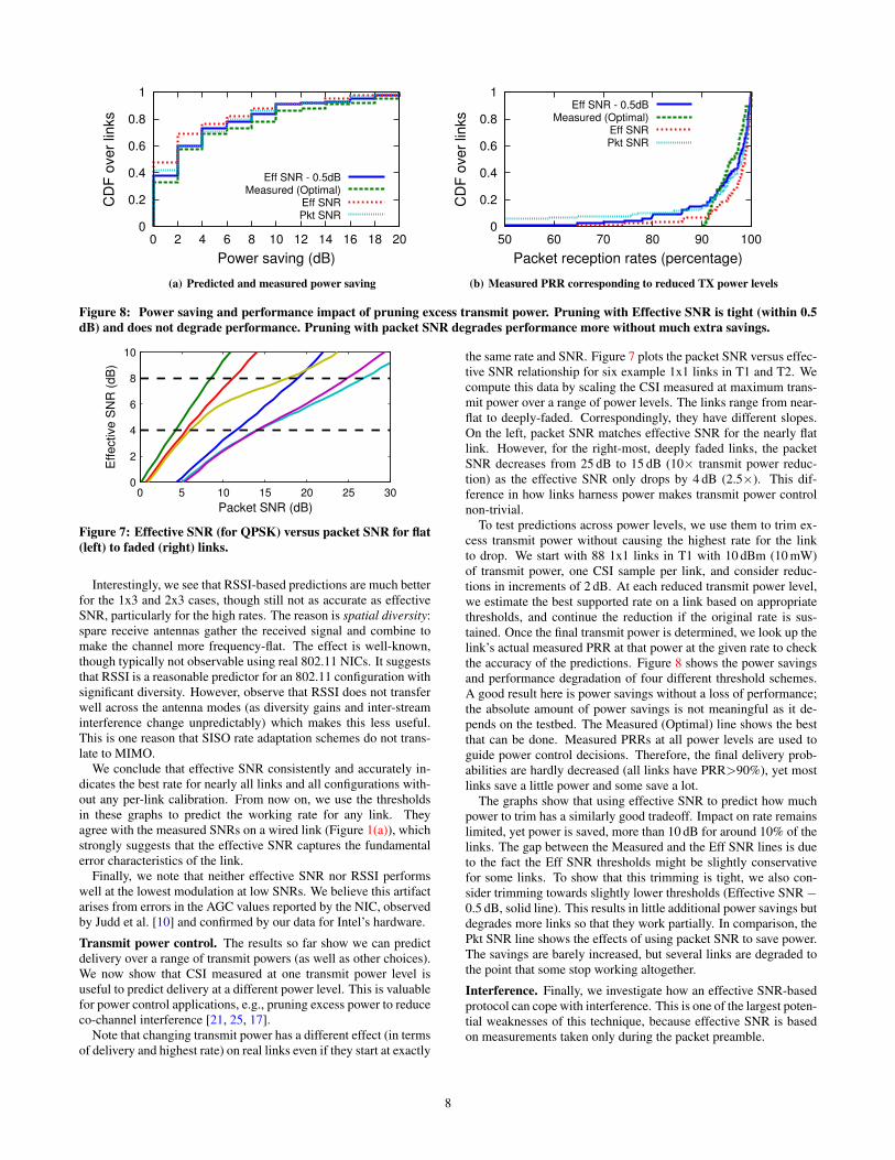
Figure 8: Power saving and performance impact of pruning excess transmit power. Pruning with Effective SNR is tight (within 0.5dB) and does not degrade performance. Pruning with packet SNR degrades performance more without much extra savings.

0 5 10 15 20 25 300

2

4

6

8

10

Packet SNR (dB)

Effective S

NR

(dB

)

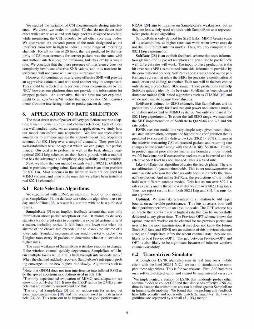
Figure 7: Effective SNR (for QPSK) versus packet SNR for flat(left) to faded (right) links.

Interestingly, we see that RSSI-based predictions are much betterfor the 1x3 and 2x3 cases, though still not as accurate as effectiveSNR, particularly for the high rates. The reason is spatial diversity:spare receive antennas gather the received signal and combine tomake the channel more frequency-flat. The effect is well-known,though typically not observable using real 802.11 NICs. It suggeststhat RSSI is a reasonable predictor for an 802.11 configuration withsignificant diversity. However, observe that RSSI does not transferwell across the antenna modes (as diversity gains and inter-streaminterference change unpredictably) which makes this less useful.This is one reason that SISO rate adaptation schemes do not trans-late to MIMO.

We conclude that effective SNR consistently and accurately in-dicates the best rate for nearly all links and all configurations with-out any per-link calibration. From now on, we use the thresholdsin these graphs to predict the working rate for any link. Theyagree with the measured SNRs on a wired link (Figure 1(a)), whichstrongly suggests that the effective SNR captures the fundamentalerror characteristics of the link.

Finally, we note that neither effective SNR nor RSSI performswell at the lowest modulation at low SNRs. We believe this artifactarises from errors in the AGC values reported by the NIC, observedby Judd et al. [10] and confirmed by our data for Intel’s hardware.

Transmit power control. The results so far show we can predictdelivery over a range of transmit powers (as well as other choices).We now show that CSI measured at one transmit power level isuseful to predict delivery at a different power level. This is valuablefor power control applications, e.g., pruning excess power to reduceco-channel interference [21, 25, 17].

Note that changing transmit power has a different effect (in termsof delivery and highest rate) on real links even if they start at exactly

the same rate and SNR. Figure 7 plots the packet SNR versus effec-tive SNR relationship for six example 1x1 links in T1 and T2. Wecompute this data by scaling the CSI measured at maximum trans-mit power over a range of power levels. The links range from near-flat to deeply-faded. Correspondingly, they have different slopes.On the left, packet SNR matches effective SNR for the nearly flatlink. However, for the right-most, deeply faded links, the packetSNR decreases from 25 dB to 15 dB (10× transmit power reduc-tion) as the effective SNR only drops by 4 dB (2.5×). This dif-ference in how links harness power makes transmit power controlnon-trivial.

To test predictions across power levels, we use them to trim ex-cess transmit power without causing the highest rate for the linkto drop. We start with 88 1x1 links in T1 with 10 dBm (10 mW)of transmit power, one CSI sample per link, and consider reduc-tions in increments of 2 dB. At each reduced transmit power level,we estimate the best supported rate on a link based on appropriatethresholds, and continue the reduction if the original rate is sus-tained. Once the final transmit power is determined, we look up thelink’s actual measured PRR at that power at the given rate to checkthe accuracy of the predictions. Figure 8 shows the power savingsand performance degradation of four different threshold schemes.A good result here is power savings without a loss of performance;the absolute amount of power savings is not meaningful as it de-pends on the testbed. The Measured (Optimal) line shows the bestthat can be done. Measured PRRs at all power levels are used toguide power control decisions. Therefore, the final delivery prob-abilities are hardly decreased (all links have PRR>90%), yet mostlinks save a little power and some save a lot.

The graphs show that using effective SNR to predict how muchpower to trim has a similarly good tradeoff. Impact on rate remainslimited, yet power is saved, more than 10 dB for around 10% of thelinks. The gap between the Measured and the Eff SNR lines is dueto the fact the Eff SNR thresholds might be slightly conservativefor some links. To show that this trimming is tight, we also con-sider trimming towards slightly lower thresholds (Effective SNR−0.5 dB, solid line). This results in little additional power savings butdegrades more links so that they work partially. In comparison, thePkt SNR line shows the effects of using packet SNR to save power.The savings are barely increased, but several links are degraded tothe point that some stop working altogether.

Interference. Finally, we investigate how an effective SNR-basedprotocol can cope with interference. This is one of the largest poten-tial weaknesses of this technique, because effective SNR is basedon measurements taken only during the packet preamble.

8

We studied the variation of CSI measurements during interfer-ence. We chose two nodes in testbed T2 that do not detect eachother with carrier sense and sent large packets designed to collide,while monitoring the CSI recorded by all other receiving nodes.We also varied the transmit power of the node designated as theinterferer from low to high to induce a large range of interferingchannels. For all but one of 20 links, the rate predicted by the ma-jority of CSI measurements for correct packets was the same withand without interference; the remaining link was off by a singlerate. We conclude that the mere presence of interference does notcompletely invalidate effective SNR values, and thus transient in-terference will not cause wild swings in transmit rate.

However, for continuous interference effective SNR will providean aggressive estimate, and will need another way to compensate.This should be reflected in larger noise floor measurements by theNIC,4 however our platform does not provide this information fordropped packets. An alternative, that we have not yet explored,might be an effective SINR metric that incorporates CSI measure-ments from the interfering nodes to predict packet delivery.

6. APPLICATION TO RATE SELECTIONThe most direct uses of packet delivery predictions are rate adap-

tion, transmit power control, and channel selection. Each of theseis a well-studied topic. As an example application, we study howour model can inform rate adaptation. We first use trace-drivensimulation to compare against the state-of-the-art rate adaptationschemes for 802.11a/g over a range of channels. They provide awell-established baseline against which we can gauge our perfor-mance. Our goal is to perform as well as the best, already near-optimal 802.11a/g schemes on their home ground, with a methodthat has the advantages of simplicity, deployability, and generality.

Next, we show that our method extends well to 802.11n (MIMO)and so provides ongoing value. Rate adaptation is an open problemfor 802.11n. Most schemes in the literature were not designed forMIMO systems, and none of the ones that were have been tested onreal 802.11 channels.5

6.1 Rate Selection AlgorithmsWe experiment with ESNR, an algorithm based on our model,

plus SampleRate [5], the de facto rate selection algorithm in use to-day, and SoftRate [28], a research algorithm with the best publishedresults.

SampleRate [5] is an implicit feedback scheme that uses onlyinformation about packet reception or loss. It maintains deliverystatistics for different rates to compute the expected airtime to senda packet, including retries. It falls back to a lower rate when theairtime of the chosen rate exceeds (due to losses) the airtime of alower rate. Standard implementations send a packet to probe 1 or2 higher rates every 10 packets, to determine whether to switch tohigher rates.

The main weakness of SampleRate is its slow reaction to change.If the wireless channel quickly degenerates, SampleRate will in-cur multiple losses while it falls back through intermediate rates.6

When the channel suddenly recovers, SampleRate’s infrequent prob-ing converges to the new highest rate slowly. Algorithms such as4Note that OFDM does not turn interference into inflated RSSI asdo the spread spectrum modulations used in 802.11b.5The only experimental evaluation of MIMO rate adaptation weknow of is on Hydra [12]. It uses the USRP radios for 2 MHz chan-nels that are relatively narrowband and flat.6The original SampleRate [5] did not reduce rate for retries, butsome implementations [10] and the version used in modern ker-nels [24] do. This turns out to be important for good performance.

RRAA [29] aim to improve on SampleRate’s weaknesses, but asthey are less widely used we stick with SampleRate as a represen-tative probe-based algorithm.

SampleRate is only defined for SISO links. MIMO breaks someof its assumptions, as higher rates can work when lower ones donot due to different antenna modes. Thus, we only compare it for802.11a/g experiments.

SoftRate [28] is an explicit feedback scheme that uses informa-tion gleaned during packet reception at a given rate to predict howwell different rates will work. The input to these predictions is thebit error rate (BER) as estimated from side-information provided bythe convolutional decoder. SoftRate chooses rates based on the per-formance curves that relate the BERs for one rate (a combination ofmodulation and coding) to another. Each rate will be the best choiceonly during a predictable BER range. These predictions can helpSoftRate quickly identify the best rate. SoftRate has been shown todominate trained SNR-based algorithms such as CHARM [10] andwe do not evaluate against those directly.

SoftRate is defined for SISO channels, like SampleRate, and itspredictions hold only for fixed transmit power and antenna modes,so it does not extend to MIMO systems. We only compare it for802.11a/g experiments. To cover the full SISO range, we extendedthe MIT implementation of SoftRate to QAM-64 and 2/3 and 5/6rate codes.

ESNR uses our model in a very simple way: given recent chan-nel state information, compute the highest rate configuration that ispredicted to successfully deliver packets (PRR > 90%). It runs atthe receiver, measuring CSI on received packets and returning ratechanges to the sender along with the ACK like SoftRate. Finally,to protect against poor choices near a rate boundary in our model,we fall back one rate if consecutive packets must be retried and theeffective SNR level has not changed. This is a fixed rule.

Like SoftRate, our algorithm obviates the search phase. There isno calibration of dynamic thresholds. This is not rate adaptation somuch as rate selection that changes only because it tracks the chan-nel’s evolution. And unlike SoftRate, the predictions of our modelhold over different antenna modes. This lets us run over 802.11nrates as easily and in the same way that we run over 802.11a/g rates.Thus, we report results from both 802.11a/g and 802.11n runs forour algorithm.

Optimal. We also take advantage of simulation to add upperbounds on achievable performance. This lets us assess how wellthe algorithms perform on an absolute scale. The OPT scheme hasan oracle that knows the true highest rate that can be successfullydelivered at any given time. The Previous-OPT scheme knows theoptimal rate that worked on the channel for the previous packet anduses it for the next transmission; it just does not know the future.Since SoftRate and ESNR use an estimate of this previous channelstate, and SampleRate infers the recent channel state, they are un-likely to beat Previous-OPT. The gap between Previous-OPT andOPT is also likely to be significant because of inherent wirelesschannel variability.

6.2 Trace-driven SimulatorAlthough our ESNR algorithm runs in real time on a mobile

client with the Intel 802.11 NIC,7 we turn to simulations to com-pare these algorithms. This is for two reasons. First, SoftRate runson a software-defined radio, and cannot be implemented on a cur-7We implemented a version of ESNR that randomly probes otherantenna modes to collect CSI and that also sends effective SNR es-timates back to the transmitter, and ran it online against SampleRatein human-scale mobility. We found that the probing and feedbackhave little penalty, and our results match the simulator: the two al-gorithms are separated by a small (5–10%) margin.

9

rently available commercial NIC. Second, we want to compare thealgorithms over varied channel conditions, from static to rapidlychanging, to assess how consistently they perform. For example,no algorithm will beat SampleRate by a significant margin on staticchannels, because it will quickly adapt to the channel. In contrast,SoftRate performs well even when the channel is changing rapidlydue to mobility. However, it is hard to generate controllable high-mobility experimental settings.

Trace. We collect real channel information for the simulations. Amobile client in T1 that is moved at normal walking speed sendsshort, back-to-back packets to stationary testbed nodes that recordthe CSI. The CSI reflects frequency-selective fading over real, vary-ing 20 MHz MIMO channels that is typically not observed withmore narrowband experimentation, e.g., on the USRP. Note thatCSI is estimated during the preamble of the packet transmission,independent of the modulation and coding of the payload. There-fore, the mobile transmitter can quickly cycle through all antennaconfigurations (1x3, 2x3 and 3x3) by sending a single short UDPpacket at the lowest rate for each configuration. This enables finegrained sampling of the channel every 650µs. The following re-sults are derived from a trace with approximately 85,000 channelmeasurements taken over 55 seconds, spanning varying RF chan-nels that range from the best 3-stream rates to SISO speeds.

Simulator. We feed this trace to a custom 802.11a/g/n simulatorwritten in a combination of MATLAB and the MIT C++ GNU Ra-dio code. The simulator implements packet reception as shownin Figure 3, including demodulation for BPSK through QAM-64,deinterleaving, and convolutional decoding with soft inputs and softoutputs. The measured CSI is interpolated to 56 carriers and servesas the ground truth for the channel, and packets are correctly re-ceived when there are no bit errors, or are lost. SampleRate, Soft-Rate, and ESNR are implemented as described previously. To en-sure that ESNR is not given the unrealistic advantage of groundtruth CSI, we corrupt the CSI at the level of ADC quantization,which typically induces an error of ±1.5 dB in the output effectiveSNRs. SoftRate estimates the BER directly during decoding.

To vary mobility, we replay the trace at different speeds. For ex-ample, 4× mobility gives ESNR the CSI from every fourth tracerecord. However, packet reception still uses all trace records. Fora packet to be correctly received in the accelerated trace, it mustbe received over the intermediate records. We require correct re-ception at ≥80% of the records to allow for coding. This modelsa varying channel that we can only sample for CSI periodically, ashappens when CSI is measured during the packet preamble. Soft-Rate operates using the 80th percentile soft estimate from the range.

We aim to evaluate the ability of these algorithms to respond tochanging channel conditions. Thus, our primary metric is the de-livered PHY layer rate per trace index. Higher-layer factors such asMAC backoff, link-layer packet aggregation, and TCP reactions toloss, will affect how this rate translates to throughput.

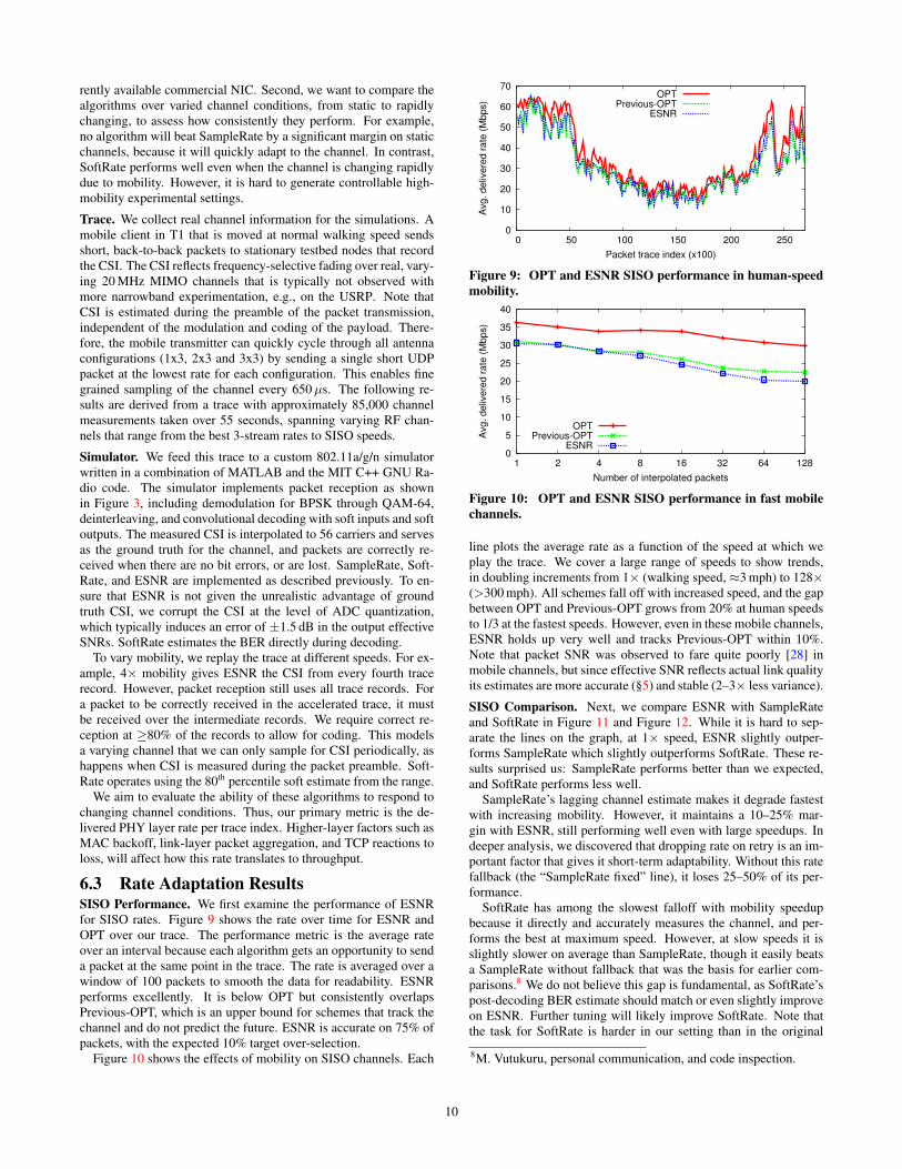
6.3 Rate Adaptation ResultsSISO Performance. We first examine the performance of ESNRfor SISO rates. Figure 9 shows the rate over time for ESNR andOPT over our trace. The performance metric is the average rateover an interval because each algorithm gets an opportunity to senda packet at the same point in the trace. The rate is averaged over awindow of 100 packets to smooth the data for readability. ESNRperforms excellently. It is below OPT but consistently overlapsPrevious-OPT, which is an upper bound for schemes that track thechannel and do not predict the future. ESNR is accurate on 75% ofpackets, with the expected 10% target over-selection.

Figure 10 shows the effects of mobility on SISO channels. Each

0

10

20

30

40

50

60

70

0 50 100 150 200 250

Avg. deliv

ere

d r

ate

(M

bps)

Packet trace index (x100)

OPTPrevious-OPT

ESNR

Figure 9: OPT and ESNR SISO performance in human-speedmobility.

0

5

10

15

20

25

30

35

40

1 2 4 8 16 32 64 128

Avg. deliv

ere

d r

ate

(M

bps)

Number of interpolated packets

OPTPrevious-OPT

ESNR

Figure 10: OPT and ESNR SISO performance in fast mobilechannels.

line plots the average rate as a function of the speed at which weplay the trace. We cover a large range of speeds to show trends,in doubling increments from 1× (walking speed,≈3 mph) to 128×(>300 mph). All schemes fall off with increased speed, and the gapbetween OPT and Previous-OPT grows from 20% at human speedsto 1/3 at the fastest speeds. However, even in these mobile channels,ESNR holds up very well and tracks Previous-OPT within 10%.Note that packet SNR was observed to fare quite poorly [28] inmobile channels, but since effective SNR reflects actual link qualityits estimates are more accurate (§5) and stable (2–3× less variance).

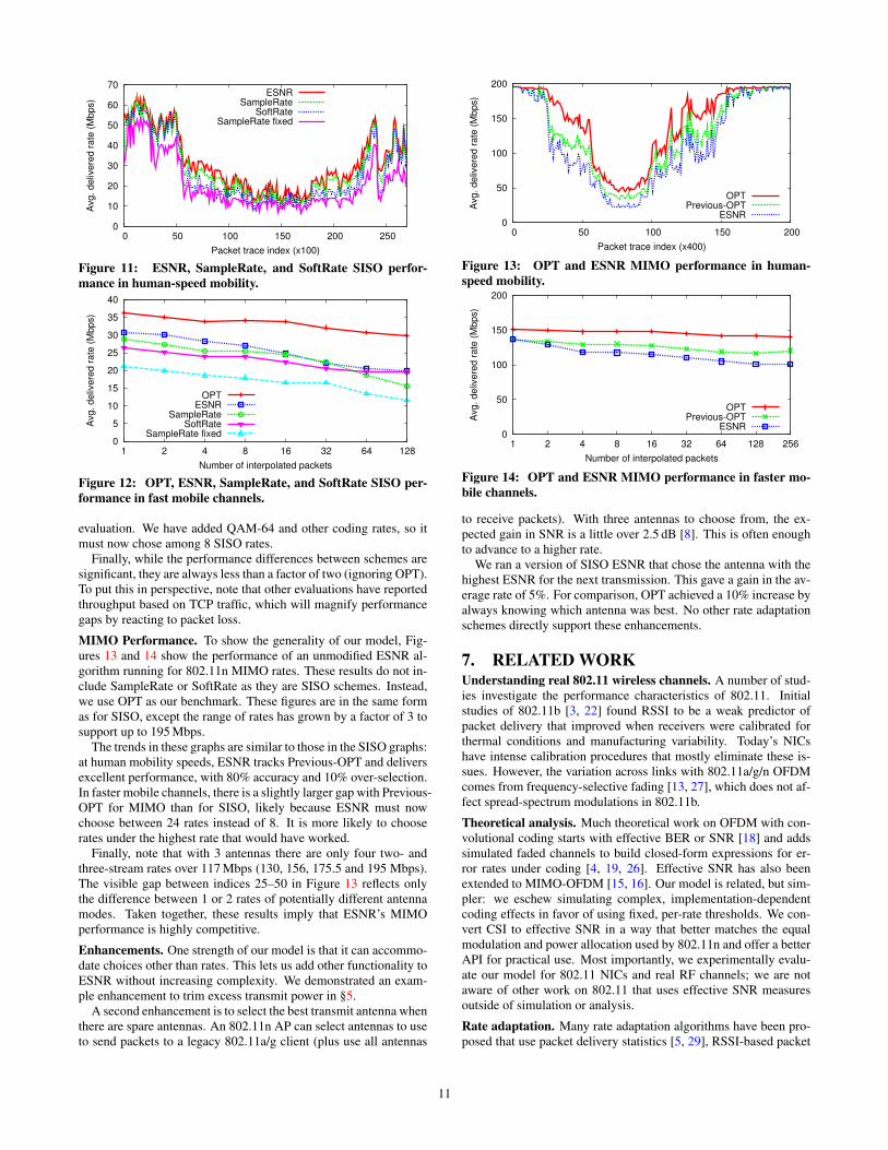
SISO Comparison. Next, we compare ESNR with SampleRateand SoftRate in Figure 11 and Figure 12. While it is hard to sep-arate the lines on the graph, at 1× speed, ESNR slightly outper-forms SampleRate which slightly outperforms SoftRate. These re-sults surprised us: SampleRate performs better than we expected,and SoftRate performs less well.

SampleRate’s lagging channel estimate makes it degrade fastestwith increasing mobility. However, it maintains a 10–25% mar-gin with ESNR, still performing well even with large speedups. Indeeper analysis, we discovered that dropping rate on retry is an im-portant factor that gives it short-term adaptability. Without this ratefallback (the “SampleRate fixed” line), it loses 25–50% of its per-formance.

SoftRate has among the slowest falloff with mobility speedupbecause it directly and accurately measures the channel, and per-forms the best at maximum speed. However, at slow speeds it isslightly slower on average than SampleRate, though it easily beatsa SampleRate without fallback that was the basis for earlier com-parisons.8 We do not believe this gap is fundamental, as SoftRate’spost-decoding BER estimate should match or even slightly improveon ESNR. Further tuning will likely improve SoftRate. Note thatthe task for SoftRate is harder in our setting than in the original

8M. Vutukuru, personal communication, and code inspection.

10

0

10

20

30

40

50

60

70

0 50 100 150 200 250

Avg. deliv

ere

d r

ate

(M

bps)

Packet trace index (x100)

ESNRSampleRate

SoftRateSampleRate fixed

Figure 11: ESNR, SampleRate, and SoftRate SISO perfor-mance in human-speed mobility.

0

5

10

15

20

25

30

35

40

1 2 4 8 16 32 64 128

Avg. deliv

ere

d r

ate

(M

bps)

Number of interpolated packets

OPTESNR

SampleRateSoftRate

SampleRate fixed

Figure 12: OPT, ESNR, SampleRate, and SoftRate SISO per-formance in fast mobile channels.

evaluation. We have added QAM-64 and other coding rates, so itmust now chose among 8 SISO rates.

Finally, while the performance differences between schemes aresignificant, they are always less than a factor of two (ignoring OPT).To put this in perspective, note that other evaluations have reportedthroughput based on TCP traffic, which will magnify performancegaps by reacting to packet loss.

MIMO Performance. To show the generality of our model, Fig-ures 13 and 14 show the performance of an unmodified ESNR al-gorithm running for 802.11n MIMO rates. These results do not in-clude SampleRate or SoftRate as they are SISO schemes. Instead,we use OPT as our benchmark. These figures are in the same formas for SISO, except the range of rates has grown by a factor of 3 tosupport up to 195 Mbps.

The trends in these graphs are similar to those in the SISO graphs:at human mobility speeds, ESNR tracks Previous-OPT and deliversexcellent performance, with 80% accuracy and 10% over-selection.In faster mobile channels, there is a slightly larger gap with Previous-OPT for MIMO than for SISO, likely because ESNR must nowchoose between 24 rates instead of 8. It is more likely to chooserates under the highest rate that would have worked.

Finally, note that with 3 antennas there are only four two- andthree-stream rates over 117 Mbps (130, 156, 175.5 and 195 Mbps).The visible gap between indices 25–50 in Figure 13 reflects onlythe difference between 1 or 2 rates of potentially different antennamodes. Taken together, these results imply that ESNR’s MIMOperformance is highly competitive.

Enhancements. One strength of our model is that it can accommo-date choices other than rates. This lets us add other functionality toESNR without increasing complexity. We demonstrated an exam-ple enhancement to trim excess transmit power in §5.

A second enhancement is to select the best transmit antenna whenthere are spare antennas. An 802.11n AP can select antennas to useto send packets to a legacy 802.11a/g client (plus use all antennas

0

50

100

150

200

0 50 100 150 200

Avg. deliv

ere

d r

ate

(M

bps)

Packet trace index (x400)

OPTPrevious-OPT

ESNR

Figure 13: OPT and ESNR MIMO performance in human-speed mobility.

0

50

100

150

200

1 2 4 8 16 32 64 128 256

Avg. deliv

ere

d r

ate

(M

bps)

Number of interpolated packets

OPTPrevious-OPT

ESNR

Figure 14: OPT and ESNR MIMO performance in faster mo-bile channels.

to receive packets). With three antennas to choose from, the ex-pected gain in SNR is a little over 2.5 dB [8]. This is often enoughto advance to a higher rate.

We ran a version of SISO ESNR that chose the antenna with thehighest ESNR for the next transmission. This gave a gain in the av-erage rate of 5%. For comparison, OPT achieved a 10% increase byalways knowing which antenna was best. No other rate adaptationschemes directly support these enhancements.

7. RELATED WORKUnderstanding real 802.11 wireless channels. A number of stud-ies investigate the performance characteristics of 802.11. Initialstudies of 802.11b [3, 22] found RSSI to be a weak predictor ofpacket delivery that improved when receivers were calibrated forthermal conditions and manufacturing variability. Today’s NICshave intense calibration procedures that mostly eliminate these is-sues. However, the variation across links with 802.11a/g/n OFDMcomes from frequency-selective fading [13, 27], which does not af-fect spread-spectrum modulations in 802.11b.

Theoretical analysis. Much theoretical work on OFDM with con-volutional coding starts with effective BER or SNR [18] and addssimulated faded channels to build closed-form expressions for er-ror rates under coding [4, 19, 26]. Effective SNR has also beenextended to MIMO-OFDM [15, 16]. Our model is related, but sim-pler: we eschew simulating complex, implementation-dependentcoding effects in favor of using fixed, per-rate thresholds. We con-vert CSI to effective SNR in a way that better matches the equalmodulation and power allocation used by 802.11n and offer a betterAPI for practical use. Most importantly, we experimentally evalu-ate our model for 802.11 NICs and real RF channels; we are notaware of other work on 802.11 that uses effective SNR measuresoutside of simulation or analysis.

Rate adaptation. Many rate adaptation algorithms have been pro-posed that use packet delivery statistics [5, 29], RSSI-based packet

11

SNR [6, 10], or symbol-level details of packet reception [23, 28] toadapt to varying channel conditions. Some proposals require cus-tom hardware [6] and may drastically change the fundamentals ofthe communication [20]. These methods do not extend to 802.11nand do not address related factors, e.g., transmit power.

Compared to SoftRate’s [28] use of BER estimates, our effec-tive SNR metric is more general. With a single CSI measurement,we can extrapolate performance in a wide space of rates, spatialstreams, antenna selections, channel widths, and transmit powerlevels. We have also shown that effective SNR can be implementedon commodity NICs and evaluated it over real wireless channelswith mobile and fixed clients. Like RRAA [29] and SoftRate, ef-fective SNR helps to distinguish collisions from channel inducedpacket loss; with accurate predictions of interference-free packetdelivery there is no need to adapt rate in response to loss.

Finally, effective SNR could inform and improve schemes thatcombine transmission with more efficient channel-dependent cod-ing [14] or partially-correct ARQ schemes [9]. Our deeper under-standing of fading should also aid attempts to use the faster OFDMrates in challenging outdoor mobile environments [7].

Transmit power control. Existing proposals for transmit powercontrol require complex probing and adaptation mechanisms [17,21, 25]. Our example in §5 suggests that, with a good predictivemodel, we can directly and confidently select a reduced transmitpower without degrading link performance.

8. CONCLUSIONWireless links are easy to understand in theory, but difficult to

operate in practice, thus search is used to find the best rates, powerlevels, or other parameter of interest. We have presented a practi-cal 802.11 packet delivery model that greatly simplifies this situa-tion. Our model takes as input the RF channel (measured as 802.11Channel State Information) and predicts whether the link will de-liver packets for a wide range of NIC configurations. It uses thenotion of effective SNR to handle OFDM over faded links, worksfor MIMO configurations, and needs no calibration of target links.

We evaluated our model experimentally with Intel 802.11a/g/nNICs. We show that, for the first time, measurements taken bycommodity NICs can accurately predict whether links will workover a wide range of rates, transmit power, spatial streams, and an-tennas settings that have not previously been tested. In contrast,predictions based on RSSI often confuse from two to five rates asthe potential best rate to use.

Our model is simple, involving only computation on channelmeasurements. It is easy to deploy, working with measurementsfrom 802.11n NICs. And it is general, working for 802.11n (MIMO)systems as well as 802.11a/g (SISO) ones. As one application, weuse it to predict the highest transmit rate for a link. Simulationsdriven by real channel measurements show that our scheme is asgood as the best 802.11a/g rate adaptation schemes, and extendsgood performance to 802.11n. We hope our model will prove use-ful for many tasks ranging from antenna and channel selection torate and transmit power control.

AcknowledgmentsWe thank our shepherd, Patrick Thiran, and the rest of the anony-mous reviewers for their helpful feedback. Tom Anderson, Shyam-nath Gollakota, and Ratul Mahajan also provided insightful com-ments on this work. We are grateful to Mythili Vutukuru for ac-cess to the SoftRate source code. This work was supported in partby an Intel Foundation Ph.D. Fellowship and by NSF grants CNS-0435065 and CNS-0722004.

9. REFERENCES[1] IEEE Std. 802.11n-2009: Enhancements for higher throughput.[2] Intel Wireless WiFi Link drivers for Linux.

http://intellinuxwireless.org.[3] D. Aguayo et al. Link-level measurements from an 802.11b mesh

network. In ACM SIGCOMM, 2004.[4] O. Awoniyi and F. A. Tobagi. Packet error rate in OFDM-based

wireless LANs operating in frequency selective channels. IEEEINFOCOM, 2006.

[5] J. C. Bicket. Bit-rate selection in wireless networks. Master’s thesis,MIT, 2005.

[6] J. Camp and E. Knightly. Modulation rate adaptation in urban andvehicular environments: cross-layer implementation andexperimental evaluation. In ACM MobiCom, 2008.

[7] J. Eriksson, H. Balakrishnan, and S. Madden. Cabernet: Vehicularcontent delivery using WiFi. In ACM MobiCom, 2008.

[8] A. Goldsmith. Wireless Communications. Cambridge UniversityPress, 2005.

[9] K. Jamieson and H. Balakrishnan. PPR: Partial packet recovery forwireless networks. In ACM SIGCOMM, 2007.

[10] G. Judd, X. Wang, and P. Steenkiste. Efficient channel-aware rateadaptation in dynamic environments. In ACM MobiSys, 2008.

[11] S. Kant and T. L. Jensen. Fast link adaptation for IEEE 802.11n.Master’s thesis, Aalborg University, 2007.

[12] W. Kim et al. An experimental evaluation of rate adaptation formulti-antenna systems. In IEEE INFOCOM, 2009.

[13] M. Lampe et al. Misunderstandings about link adaptation forfrequency selective fading channels. In IEEE PIMRC, 2002.

[14] K. C.-J. Lin, N. Kushman, and D. Katabi. ZipTx: Harnessing partialpackets in 802.11 networks. In ACM MobiCom, 2008.

[15] H. Liu, L. Cai, H. Yang, and D. Li. EESM based link error predictionfor adaptive MIMO-OFDM system. In IEEE VTC, 2007.

[16] G. Martorell, F. Riera-Palou, and G. Femenias. Cross-layer linkadaptation for IEEE 802.11n. In Cross Layer Design (IWCLD), 2009.

[17] J. P. Monks, V. Bharghavan, and W. M. W. Hwu. A power controlledmultiple access protocol for wireless packet networks. In IEEEINFOCOM, 2001.

[18] S. Nanda and K. M. Rege. Frame error rates for convolutional codeson fading channels and the concept of effective Eb/N0. In IEEEVTC, 1998.

[19] Nortel Networks. Effective SIR computation for OFDM system-levelsimulations. 3GPP TSG RAN WG1 #35, R1-031370, 2003.

[20] H. Rahul, F. Edalat, D. Katabi, and C. Sodini. Frequency-aware rateadaptation and MAC protocols. In ACM MobiCom, 2009.

[21] K. Ramachandran, R. Kokku, H. Zhang, and M. Gruteser. Symphony:synchronous two-phase rate and power control in 802.11 WLANs. InACM MobiSys, 2008.

[22] C. Reis, R. Mahajan, M. Rodrig, D. Wetherall, and J. Zahorjan.Measurement-based models of delivery and interference in staticwireless networks. In ACM SIGCOMM, 2006.

[23] S. Sen, N. Santhapuri, R. R. Choudhury, and S. Nelakuditi.AccuRate: Constellation based rate estimation in wireless networks.In USENIX NSDI, 2010.

[24] D. Smithies and F. Fietkau. minstrel: MadWiFi and Linux kernel rateselection algorithm, 2005.

[25] D. Son, B. Krishnamachari, and J. Heidemann. Experimental study ofthe effects of transmission power control and blacklisting in wirelesssensor networks. In IEEE SECON, 2004.

[26] V. Tralli. Efficient simulation of frame and bit error rate in wirelesssystems with convolutional codes and correlated fading channels.IEEE WCNC, 1999.

[27] D. Tse and P. Viswanath. Fundamentals of Wireless Communication.Cambridge University Press, 2005.

[28] M. Vutukuru, H. Balakrishnan, and K. Jamieson. Cross-layer wirelessbit rate adaptation. In ACM SIGCOMM, 2009.

[29] S. H. Y. Wong, H. Yang, S. Lu, and V. Bharghavan. Robust rateadaptation for 802.11 wireless networks. In ACM MobiCom, 2006.

[30] J. Zhang et al. A practical SNR-guided rate adaptation. In IEEEINFOCOM, 2008.

[31] J. Zhao and R. Govindan. Understanding packet delivery performancein dense wireless sensor networks. In ACM SenSys, 2003.

12