Embed Size (px)
Citation preview

Predictability: the wrong wayAndrea Buraschi and Andrea Carnelli
First draft: November 2011This version: May 2012
ABSTRACT
We study the predictability of S&P500 returns using short term expected risk premia as aconditioning variable. We construct short term expected risk premia by combining dividendprices implied by futures markets with a simple model of dividend expectations. Regressionresults for forecasting horizons from 1 to 4 quarters show that time variation in risk premiacaptures time variation in realized excess returns, albeit with the wrong sign. Counter to theintuition that a high price of risk commands high returns, we find that high expected returnspredict low returns. The economic significance is strong: a one standard deviation rise inexpected risk premia decreases realized excess returns by 0.16 (0.34) standard deviations atquarterly (annual) horizons. No asset pricing model is able to generate these patterns ofpredictability.
Keywords: equity risk premium, predictability, dividend prices, asset pricing models, termstructure.JEL Codes: G10, G12, G13.
Andrea Buraschi ([email protected]) is at The University of Chicago Booth School of Business.Andrea Carnelli ([email protected]) is at Imperial College London Business School.

I Introduction
In this paper we construct an empirical proxy for short term expected risk premia and study its
empirical properties. Understanding the properties of risk premia is one of the most important yet
challenging tasks in asset pricing. One of the challenges is related to the fact that, in general, it
is difficult to identify risk premia demanded by investors: they cannot be directly observed when
the timing and magnitudes of dividends are unknown. A stock index pays uncertain dividends at
uncertain times over a life of uncertain duration. Investors form expectations about future cash
flows and use a set of discount rates to determine the value. All information is then aggregated by
a tatonnement and the econometrician can only observe a time series of stock prices. This “loss”
of information is a binding constraint for our understanding of asset prices; its limits are laid bare
when contrasted to our understanding of discount rates in fixed income markets. In the fixed
income literature, the term structure of interest rates is an observable entity with two important
roles. First, it encodes information about the dynamics of the stochastic discount factor (yields
are risk adjusted expectations of future short rates). Second, it provides a host of restrictions that
allow to better discriminate among alternative models. If equity discount rates were observable,
we could learn about their dynamics and generate additional restrictions that asset pricing models
have to satisfy.
How can we construct a measure of expected returns? We follow the pioneering work of Van
Binsbergen et al. (2011) and address this challenge by using observations on dividend prices.
Dividend prices can be obtained by imposing a simple no-arbitrage pricing restriction on cash and
derivatives markets. The prices of dividends carry information on both future expected dividend
and risk premia. By modeling expectations about short term dividends, we are able to identify the
short term risk premium component embedded in dividend prices. We investigate the properties
of these market-implied short term risk premia (erxSTt hence). In particular, we are interested in
the relationship between erxSTt and longer maturity discount rates. We explore this relationship
indirectly by running predictive regressions of realized excess returns on lagged short term risk
1

premia. Since realized excess returns reveal changes in equity discount rates at all maturities,
these regressions allow us to uncover the dynamic link among short- and long-term discount rates.
We ask to what extent the dynamics of risk premia on short term dividends help to explain index
returns and which asset pricing model can be consistent with some of its basic properties.
We test the null hypothesis of no predictability by projecting realized excess returns on short
term expected risk premia. Our results can be summarized as follows. We find that short term
expected returns predict realized returns over short horizons. The economic significance is strong:
a one standard deviation rise in expected risk premia decreases realized excess returns by 0.16
(0.34) standard deviations at quarterly (annual) horizons. The predictive power of expected
returns over short horizon is over and above that of dividend yields: expected returns detect high
frequency predictability components in stock returns that dividend yields do not capture. Even
more interesting, the sign of the slope coefficient is negative: higher market-implied risk premia at
time t are followed by lower excess returns at time t + h. We control for the overlapping nature of
the regressions, and verify that the results are robust to potential mis-specification of the model
for expected dividends. The results are difficult to be reconciled with leading asset pricing models,
at least in their traditional specifications. These models generate risk premia dynamics and term
structures of expected equity returns that are too restrictive. We identify the two ingredients that
are necessary for a model to be able to explain this type of predictability: shocks to dividends must
be priced, and there must be a multivariate state vector driving the term structure of expected
risk premia.
Our first empirical exercise is a regression of excess returns on expected one year risk premia:
can theory say something about the sign and magnitude of the slope coefficient? The problem can
be best understood by means of an analogy to fixed income securities. We can think of an equity
index as a long maturity bond (say, 30 years) that pays coupons (i.e. dividends), and we can
think of short term expected risk premia as the yield on a short maturity (say, 1 year) zero coupon
bond. The issue we address is akin to the question: can one year yields predict one-year holding
2

period returns on a 30 years maturity bond? A rigorous answer to the question involves specifying
a term structure model that: i) derives the price of a bond as a function of state variables, and
ii) determines expected risk premia by modeling the covariance between shocks to bond prices
and shocks to the stochastic discount factor. To the extent that the yield on the 1 year bond
reveals the state variable, it is also possible to form expectations about the 1 year holding period
return of the 30 year maturity bond. An equity index is like a coupon-bearing bond, except that
is has infinite maturity and cash flow risk. Just like a coupon-bearing bond can be thought of as
a portfolio of zero coupons, an equity index is a portfolio of “zero coupon” dividend strips, i.e.
claims to dividends payable at future dates. The term structure model of dividend strips we adopt
is the one developed in Lettau and Wachter (2007). Lettau and Wachter (2007) show that short
term expected risk premia (our regressor) identify the price of risk up to a scaling factor, and that
expected returns on dividend strips with longer maturities are positive functions of the price of
risk. Since the return on the index is the sum of returns on dividend strips of all maturities, the
model provides a tight link between the left and right hand side variables of our regression, and
motivates its predictive power.
This work is especially related to Van Binsbergen et al. (2011) study of equity yields. Equity
yields are the ratio of the futures price of dividend futures to the current dividend. Time variation
in equity yields reflects time variation in dividend growth expectations and/or risk premia. The
authors test the predictive power of equity yields, and use a VAR to separate the dividend growth
from the risk premia components. They find that equity yields are good forecasters of dividend
and consumption growth, and that risk premia are counter cyclical. Our analysis is different from
Van Binsbergen et al. (2011) in two respects. First, instead of looking at the predictability of
dividend growth, we focus on the predictability of returns. Second, we exploit the predictability
of returns conditional on short term risk premia to uncover the dynamics and time dependence of
the term structure of equity risk premia.
3

II A Motivating Example
As a motivation for the regressions that follow, we use the term structure model of dividend prices
developed by Lettau and Wachter (2007) to shed light on the relationship between short term
expected risk premia and index returns. The logarithm of dividend growth dt+1 = log(Dt+1/Dt)
and its conditional mean zt+1 are assumed to follow
∆dt+1 = g + zt + σdεt+1
zt+1 = φzzt + σzεt+1.
(1)
The price of risk is driven by a state variable xt that evolves according to
xt+1 = (1 − φx)x̄ + φxxt + σxεt+1,
where εt+1 is a 3 × 1 vector of independent standard normal shocks, so that the “shock loadings”
σd, σz, σx are 1×3 row vectors. Note that the conditional volatility of each variable is given by the
norm of the vector of shock loadings, while the conditional covariance between any two variables
is given by the inner product of the respective vectors of shock loadings. Since only dividend risk
is assumed to be priced, and the (log) risk free rate rf = log Rf is assumed to be constant, the
stochastic discount factor equals
Mt+1 = exp{− rf − 1
2x2
t − xtσd
||σd||εt+1
}.
Let Pt,n be the price of a claim that pays the aggregate dividend n periods from now, and let
Rn,t+1 = Pt+1,n−1/Pt,n denote the return on holding the dividend claim for one period. Note that
by no arbitrage, it must be that Pt,0 = Dt. Lettau and Wachter (2007) show that under these
assumptions both the price-to-dividend ratio and the expected excess return on dividend claims
4

are exponential-affine functions of the state variables:
log Pt,n = log Dt + A(n) + Bx(n)xt + Bz(n)zt
log Et
[Rn,t+1/R
f]
=(σd + Bx(n − 1)σx + Bz(n − 1)σz
) σ′d
||σd||xt, (2)
where the values of the coefficients A(n), Bz(n), and Bx(n) are given by the boundary condition
for n = 0
A(0) = Bz(0) = Bx(0) = 0,
and, for n > 0, by the recursions
A(n) = A(n − 1) − rf + g + Bx(n − 1)(1 − φx)x̄ +1
2Vn−1V
′n−1
Bz(n) =1 − φn
z
1 − φz
Bx(n) = Bx(n − 1)
(φx − σx
σ′d
||σd||
)− (σd + Bz(n − 1)σz)
σ′d
||σd||.
Since an index can be thought of as a portfolio of dividend claims, its value today is equal to the
sum of the prices of the dividend strips
Pt =∞∑
n=1
Pt,n,
and the expected excess return it generates is a weighted average of dividend risk premia across
the range of maturities
log Et
[Rt+1/R
f]
= log
(∞∑
n=s
wn exp{
(σd + Bx(n − 1)σx + Bz(n − 1)σz)σ′
d
||σd||xt
}), (3)
where wn = Pn,t/Pt and s = 1 (s = 2) for cum-dividend (ex-dividend) returns.
Equations (2) and (3) allow us to gain insight into the relationship between short term expected
5

risk premia (the right hand side of our regression) and index returns (the left hand side of our
regression). Short term expected risk premia are the empirical counterpart to (2) for n = 1
log Et
[R1,t+1/R
f]
= ||σd||xt. (4)
Equation (4) says that expected risk premia backed out of short term dividend expectations and
prices are a constant multiple of the latent factor xt. Since the expected return on the index is
also a function of xt, its derivative with respect to ||σd||xt is different from zero
β1 =∂ log Et
[Rt+1/R
f]
∂||σd||xt
. (5)
Defining β0 = log Et
[Rt+1/R
f]− β1||σd||xt, and letting {ut} denote a white noise process orthog-
onal to xt, one can see that the model imposes a restriction on the coefficients of the regression
log(Rt+1/Rf ) = β0 + β1||σd||xt + ut+1, (6)
and suggests that expected risk premia on short term dividends can predict future realized returns.
Equations (??) is the core regression of our empirical exercise. The relationship lends itself to a
simple interpretation. The only risk involved in buying a claim to one-year forward dividends is
dividend volatility, so that short term expected risk premia are proportional to the latent factor
that drives the price of risk. Since the price of risk is a state variable for the entire term structure of
dividend strips, variation in short term expected risk premia captures variation in realized returns.
III Data
This section describes the data set. All data are at quarterly frequency and span the period from
1986 : 1 to 2011 : 4. The reason behind picking 1986 as a start year is data availability: since
we construct short term expected risk premia from dividend prices implied by index futures, we
can only study the period over which S&P500 futures are traded. The use of futures data also
6

motivates the choice of sampling frequency: since contract maturities are in the March quarterly
cycle, quarterly observations dispense us with the need to obtain constant maturity contracts. As
an alternative to backing out dividend prices indirectly from index futures via the cost of carry,
we could have obtained direct observations from dividend swaps, as in Binsbergen et al. (2011).
Dividend swaps have the advantage of being traded for a large range of maturities, but, at the
same time, they are OTC contracts with counter-party risk and have gained in popularity quite
some time after index futures. Also, dividend prices implied by dividend swaps are potentially
subject to price pressure owing to institutional hedging.1 Since our intention is to construct short
term expected risk premia, the trade-off between the two datasets is biased in favor of futures
data.
A Derivation of Expected Risk Premia
The price of a stock is the sum of the prices of the dividends it will pay in the future. By combining
dividend prices with dividend expectations of different maturities, it is possible to back out a term
structure of discount rates. Dividend expectations can be recovered either directly (from analysts’
forecasts) or indirectly (via an econometric model). Dividend prices on the other hand are implicit
in the spread between cash and (discounted) futures prices. More formally, consider a dividend-
paying financial asset with time t price St and a forward contract written on the asset with delivery
n periods in the future. Define Pt,n as the value that makes the cost of carry formula true:
Ft,n = [St − Pt,n] enrt,n ,
where rt,n is a (continuously compounded) risk-free rate appropriate to discount t + n cash flows
back to t. The expression can be re-written in terms of Pt,n
Pt,n = St − Ft,ne−nrt,n . (7)
1Investment banks typically sell derivatives whose payoffs are ex-dividend; hedging these derivatives requires aposition in the underlying, which gives rise to a long exposure to dividend risk. If dividend risk is too high, theinvestment bank might have the incentive to sell dividend derivatives at particularly attractive prices.
7

By no arbitrage Pt,n must be the price that markets are willing to pay for the dividend stream
between t and t + n. Equation (6) thus provides a means to infer the price of dividend claims
from spot and futures market data. Let Dt+n denote the dividend that the asset will pay at t+n.
Since Dt+n is a random variable at t, its price today is equal to its expected value discounted by
a risk free rate and an appropriate risk premium µt,n
Pt,n = Et [Dt+n] e−n(rt,n+µt,n).
Re-arranging terms, time t expected risk premia for t + n cash flows can be expressed as
µt,n =log Et[Dt+n] − log Pt,n
n− rt,n. (8)
The following sections explore the data counterparts to equations (6) and (7).
B S&P500 Dividend Prices
In order to construct term structures of dividend prices using (6) we need the time series of spot
prices St, futures prices Ft,n, and interest rates rt,n that are appropriate to discount time t + n
cash flows to t. S&P500 futures trade on the Chicago Mercantile Exchange (CME). Available
maturities vary within the sample. When S&P500 futures started trading in 1982, available
maturities included the first 4 months in the March cycle. Ever since, the number of available
contracts has increased progressively.2 All open positions are settled in cash at close of the last
day of trading (3:15 p.m. on Thursday prior to third Friday of the contract month) to the Special
Opening Quotation (SOQ). The SPQ is calculated using normal index procedures except that the
prices used are the actual opening values of the constituents. Since securities might start trading
minutes or hours after the opening bell of the NYSE, the SPQ can be significantly different than
the published opening value of the index. The SPQ is used because it represents actionable values
and thus ensures convergence of cash and futures markets.
2As of March 2012, available maturities include 11 contracts in the March cycle.
8

Both futures and spot data are taken from Thomson Datastream. There is a slight mismatch
in the timing of index and futures close prices. CME sets settlement prices for the day equal to
midpoint of the closing range based on pit trading activity between 15:14:30-15:15:00 Central Time.
S&P indices on the other hand are computed using New York Stock Exchange (NYSE) close prices
at 16:00:00, Eastern Time. The implicit assumption is that the 15 minutes mismatch in quotes
can be treated as white noise. To compute dividend prices, we use equation (6) by combining
underlying and futures prices with interest rates data from IvyDB (Optionmetrics). The database
contains (annualized, continuously compounded) zero curves derived from LIBOR rates from the
British Bankers Association (BBA) and settlement prices of Chicago Mercantile Exchange (CME)
Eurodollar futures. For a given futures contract, the appropriate interest rate corresponds to the
zero-coupon rate that has a maturity equal to the futures’ expiration date, and is obtained by
linearly interpolating between the two closest zero-coupon rates on the zero curve. 3 At the end
of each quarter, we obtain the prices of cumulative dividends for different maturities. Since we
use quarterly data, the maturities of the dividend prices we obtain are constant over time; this
allows us to dispense with the need of interpolation techniques to obtain constant maturity prices,
which would be necessary with higher sampling frequency. The number of maturities depends
on the set of available contracts. Ideally, we would like to exploit the information of the entire
term structure of dividend prices, and back out a term structure of expected risk premia. This
approach, however, has three limitations. First, the depth of the term structure varies over time,
as argued above. Second, even though the use of quarterly data virtually eliminates the possibility
of stale prices, dividend prices might still reflect, to some extent, the different levels of liquidity of
the futures contracts used to construct them. Third, the prices of short-maturity dividends may
inherit the seasonality of dividend payments. Bearing these considerations in mind, we construct
dividend prices using the third available contract, which is the longest maturity contract available
over the entire sample.
3IvyDB data starts in 1996. Between 1986 and 1996, we use the term structure of monthly LIBOR rates(obtained from Datastream).
9

C S&P500 Dividend Expectations
In order to construct dividend expectations, we work under the null hypothesis that (log) dividend
growth is equal to a constant plus a white noise process. This assumption is well defended by a
large body of empirical literature. Many authors (see Cochrane, 2005, for a review) have found that
time variation in dividend yields can forecast future excess returns. It can be easily shown that,
in rational economies without bubbles, this empirical finding, coupled with an accounting identity
that relates current prices to future cash flows and discount rates, implies the absence of dividend
growth predictability (see, for instance, Cochrane 2006 and references therein). Absence of divi-
dend growth predictability can be understood as the consequence of dividend smoothing corporate
policies; importantly, it implies that time variation in the value of dividend claims is dominated by
revisions in the ”quantity” and ”price” of risk. If (log) dividend growth is equal to a constant plus
white noise, ∆dt+1 = g + σdεt+1, the level of future dividends is Dt+1 = Dt exp (g + σdεt+1), and
expected future dividends are equal to Et[Dt+1] = Dt exp(g + 1
2||σd||
). We use current dividends
Dt as a proxy of dividend expectations. The term g + 12||σd|| is a constant that is absorbed by the
intercept of our regression since we take logs of the RHS. IBES dividend forecasts would be an
ideal measure of model-free, forward-looking dividend expectations. Unfortunately, dividend per
share forecast data are well populated only since 2004. In the robustness section, however, we re-
run predictive regressions using expected risk premia constructed from IBES consensus forecasts,
and show that the results are robust. The assumption that dividend growth is a constant plus a
white noise process seems not to be rejected in our sample: the plot of ∆dt+1 in figure 1 resembles
a white noise process.
D S&P500 expected risk premia, realized returns, and dividend yields
In order to construct excess expected and realized returns, we need data on risk free rates. We
take the 3 month US Treasury rate from Datastream. Rates are quoted on a discount basis,
annualized using the 30/360-day-count convention, and expressed in percentage points. We convert
all rates to their annualized, continuously compounded equivalents using the Actual/360-day-count
10

convention. 4 We compute one-year forward expected risk premia erxSTt by combining one-year
forward dividend expectations and prices with 12 month risk-free rates via (7). Figure 2 plots the
time series of erxSTt . The plot peaks in December 2000 at a level that is economically unreasonable,
so in the analysis that follows we exclude this observation (the inclusion of the observation has the
only effect of strengthening all results). Table I reports the sample statistics: expected risk premia
are generally high (the mean is 31%) and volatile (26% standard deviation). Consistent with the
findings of Van Binsbergen et al. (2010), our measure of expected returns documents that risk
premia on short term cash flows are considerably higher than the risk premium earned historically
on the S&P500. Finally, realized excess returns rxt,t+h are constructed as the (annualized) cum-
dividend (log) return on the index between t and t + h, minus the (annualized) 3 month Treasury
rate prevailing at time t.
IV Forecasting regressions
A Baseline model
The reduced-form model presented in the first section suggests that one year expected returns
predict realized returns with a positive sign. To investigate this link empirically we run regressions
of realized excess returns on expected one-year risk premia over different forecasting horizons h:
rxt+h = β(h)0 + β
(h)1 erxST
t + ε(h)t+h. (9)
When data sampling is finer than forecasting horizons, predictive regressions are overlapping.
The overlap causes regression errors to be serially correlated even under the null hypothesis of no
predictability: estimates of the covariance matrix of coefficients based on the classic assumption of
homoskedasticity and no autocorrelation overstate the statistical significance of the estimates. In
order to rule out spurious statistical significance, we estimate the covariance matrix of coefficients
4Let R be the discount yield on a bond due in τ days. The annualized, continuously compounded, rate associatedwith R is equal to r = (365/τ) log (1 + (R/100) × (τ/360)).
11

in two ways: Newey and West (1987), and Hansen and Hodrick (1980). The two methods can be
understood as instances of the GMM framework for different choices of the long run covariance
matrix of sample moments. To illustrate, let β denote a (K × 1) vector of OLS coefficients in
the forecasting regression yt+h = xtβ′t + εt+h for t = 1, . . . , T + h. Since the OLS estimate of β
satisfies E[εt+h ⊗ xt] = 0, E[εt+h ⊗ xt] = 0 is the equivalent GMM moment condition. The benefit
of working with GMM is that it only assumes that errors are orthogonal to the regressors. The
covariance matrix of OLS estimates is
V ar [β] = E[xtx′t]−1SE[xtx
′t]−1,
where
S =∞∑
j=−∞
E[εt+hxtx
′t−jεt−j+h
].
Henceforth, we will denote Newey and West (1987) and Hansen and Hodrick (1980) errors by NW
and HH, respectively. The difference is based on alternative methods to estimate the (asymptotic)
covariance matrix of coefficients in regression (8), taking the overlaps into account.5 We consider
four forecasting horizons: 1, 2, 3, 4 quarters. For each forecasting horizon, we test for the marginal
significance of slope coefficients using NW and HH errors.
Table II contains the output of the regressions. With the exception of very short horizons, the
statistical significance of the loadings of realized excess returns on expected risk premia is high.
While the significance of the slope coefficient for one quarter horizons is just below 10%, all other
t-statistics, computed using both NW and HH errors, are significant at the 5% level. Statistical
significance tends to be increasing in forecasting horizon, and peaks at forecasting horizons of
three quarters, achieving −3.45 (NW errors) and −3.14 (HH errors). Also the adjusted R2 are
5The two methods differ in the estimation of S. Newey and West (1987) propose to underweight higher ordersample autocorrelations: S =
∑lj=−l
(h−|j|
h
) (1T
∑T+hh εt+hxtxt+h−jεt+h−j
), where the maximum number of
lags l is constrained by sample size lmax = T + h − 1. Hansen and Hodrick (1980) suggest to correct only forthe MA(h − 1) structure introduced by the overlap, and to weight autocorrelations equally: S =
∑h−1j=−h+1
1T∑T+h
h εt+hxtxt+h−jεt+h−j .
12

increasing in maturity: they range from 1.37% to 10.91%. Given the simplicity of the econometric
model and the high noise in realized returns, the degree of predictability we find is interesting.
The most striking feature of the results relates to its economic significance. Since both regres-
sands and regressors are standardized, the coefficients can be interpreted as standard deviation
changes in realized excess returns caused by a one standard deviation change in expected risk pre-
mia.The estimated coefficients over the four forecasting horizons are −0.16,−0.23,−0.30,−0.34.
In order to facilitate comparability across forecasting horizon, consider the annualized slope co-
efficients: −0.64,−0.46,−0.23,−0.34. The magnitudes are economically significant. Importantly,
contrary to the predictions of the model of Lettau and Wachter (2007), the estimated slope coef-
ficients are negative: higher levels of expected risk premia are associated with lower subsequent
realizations of excess returns.
B Horse races
A natural question is whether expected risk premia feature explanatory power over and above
that of traditional predictive variables studied by the empirical literature. A popular strand of
literature, for instance, looks at the predictive power of dividend yields. These regressions have
a strong theoretical motivation: under the assumption of rationality and non bubbles, it can be
easily shown that dividend yields can vary over time only if either dividend growth or excess
returns are predictable. Many authors find evidence that the dividend yield is a predictor of
future excess returns, and that the predictive power rises in the forecasting maturity (see, for
instance, Campbell 1991 and Cochrane 1992). Examining the joint predictive power of expected
risk premia and dividend yields is interesting for two reasons. First, since the two variables capture
time variation of future excess returns at different frequencies (we find that expected risk premia
forecast excess returns over short horizons, while dividend yields are known to have predictive
power over long horizons), a model that includes both variables can lead to better forecasting
performance. Second, by controlling for time varying expectations about all future excess returns,
13

the inclusion of dividend yields allows to isolate the role of short term expected risk premia.
Table III summarizes the evidence about dividend yield predictability in our sample, by showing
the output of forecasting regressions of realized excess returns on lagged dividend yields. (We also
include 3-month treasury rates because Ang and Bekaert (2006) find that it improves the short
term forecasting power of dividend yields). The results are consistent with the empirical literature.
Dividend yields predict excess returns with a positive sign (low prices relative to dividends capture
high discount rates, rather than low dividend growth), and forecasting power builds over longer
maturities: both the t-statistics and adjusted R2 rise monotonically with the forecasting horizon.
On the other hand, contrary to the finding of Ang and Bekaert (2006), we find that 3-month
Treasury rates do not have marginal significance.
Having run univariate regressions on erxSTt and dyt separately, we analyze their combined
predictive power in bivariate regressions:
rxt+h = β(h)0 + β
(h)1 erxt + β
(h)2 dyt + β
(h)3 rft + ε
(h)t+h. (10)
Table IV summarizes the regression results. While the inclusion of dividend yields seem to absorb
some of the forecasting power of erxSTt , the statistical significance of expected risk premia over
horizons of three and four quarters remains high: slope coefficients are significant at least at the
5% level. Controlling for dividend yields, the economic significance is only marginally affected: the
slope coefficients remain negative. The estimated coefficients over the four forecasting horizons
are −0.12,−0.18,−0.23,−0.27, or, expressed on a per annum basis, −0.48,−0.36,−0.17,−0.27:
relative to the baseline case, we still find that the annualized loadings are decreasing (in absolute
value) in the forecasting horizons, but this effect is slightly accentuated by the inclusion of dividend
yields. The loadings on dividend yields, on the other hand, still feature a statistical significance
that increases in the forecasting horizon; erxSTt seems to absorb part of its forecasting power: the
null hypothesis that the estimated slope coefficient on dyt is equal to zero can be rejected only for
14

annual horizons. The loadings on dyt are increasing in the horizon 0.09, 0.15, 0.20, 0.26.
There are three main lessons to be learned from the results of regressions 8 and 9. First,
the finding that higher expected risk premia predict lower subsequent excess returns features high
statistical and economic significance. Importantly, the finding is robust to the inclusion of dividend
yields and interest rates. Second, while expected risk premia and dividend yields feature some
commonality, marginal significance statistics suggest that they carry different information. Third,
differences in the patterns of loadings across maturities suggest that time variation in erxSTt and
dyt captures high (low) frequency components of future realized returns.
C Bond predictability
To the extent that short term risk premia on short term dividends capture the compensation
that investors require on short-term investments, it is reasonable to conjecture that they possess
forecasting ability for other asset classes. We test this conjecture by looking at the ability of short
term risk premia to predict excess returns on Treasury securities. We consider Treasury securities
for two reasons. First, bonds have a fixed maturity, so the decomposition of their returns into
short- and long-term shocks to discount factors is easier than for equities. Second, the absence of
cash flow risk allows us to focus on the “discount rate risk” component of short term risk premia.
We follow the empirical fixed income literature and run predictive regressions of annual bond
excess returns constructed from the Fama-Bliss dataset (from WRDS). Unfortunately, data lim-
itations do not allow us to consider shorter forecasting horizons. The annual excess return on a
bond with maturity n is defined as p(n−1)t+1Y − p
(n)t − y
(1)t , where p
(n)t denotes the time t log-price
of a zero discount bond with maturity in n years, and y(n)t is the yield associated with maturity
n at time t, i.e. y(n)t = −(1/n)p
(n)t . Since n -year forward spreads are known to have predictive
power for the annual returns of n-year bonds (Fama and Bliss, 1987), we include forward spreads
as controls. The n-year forward spread is defined as f(n)t − y
(1)t , where f
(n)t = p
(n−1)t − p
(n)t .
15
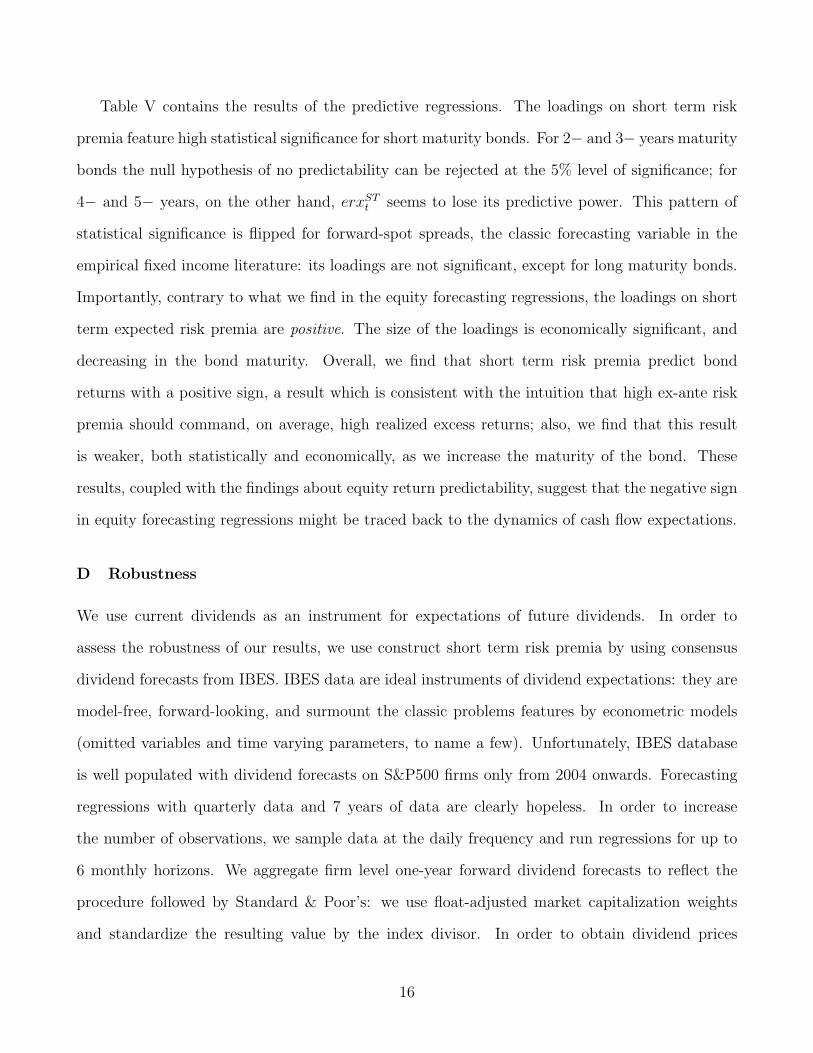
Table V contains the results of the predictive regressions. The loadings on short term risk
premia feature high statistical significance for short maturity bonds. For 2− and 3− years maturity
bonds the null hypothesis of no predictability can be rejected at the 5% level of significance; for
4− and 5− years, on the other hand, erxSTt seems to lose its predictive power. This pattern of
statistical significance is flipped for forward-spot spreads, the classic forecasting variable in the
empirical fixed income literature: its loadings are not significant, except for long maturity bonds.
Importantly, contrary to what we find in the equity forecasting regressions, the loadings on short
term expected risk premia are positive. The size of the loadings is economically significant, and
decreasing in the bond maturity. Overall, we find that short term risk premia predict bond
returns with a positive sign, a result which is consistent with the intuition that high ex-ante risk
premia should command, on average, high realized excess returns; also, we find that this result
is weaker, both statistically and economically, as we increase the maturity of the bond. These
results, coupled with the findings about equity return predictability, suggest that the negative sign
in equity forecasting regressions might be traced back to the dynamics of cash flow expectations.
D Robustness
We use current dividends as an instrument for expectations of future dividends. In order to
assess the robustness of our results, we use construct short term risk premia by using consensus
dividend forecasts from IBES. IBES data are ideal instruments of dividend expectations: they are
model-free, forward-looking, and surmount the classic problems features by econometric models
(omitted variables and time varying parameters, to name a few). Unfortunately, IBES database
is well populated with dividend forecasts on S&P500 firms only from 2004 onwards. Forecasting
regressions with quarterly data and 7 years of data are clearly hopeless. In order to increase
the number of observations, we sample data at the daily frequency and run regressions for up to
6 monthly horizons. We aggregate firm level one-year forward dividend forecasts to reflect the
procedure followed by Standard & Poor’s: we use float-adjusted market capitalization weights
and standardize the resulting value by the index divisor. In order to obtain dividend prices
16

with constant time to maturity, we interpolate linearly between available contracts. Table VI
summarizes the results: the slope coefficients on erxSTt are statistically significant and negative.
Bearing in mind the short span of the sample and the high frequency of the regressions, also
these regressions confirm the robustness of our results to potential misspecification of the model
of dividend expectations.
V Understanding predictability
The finding that expected risk premia predict realized returns with a negative sign is puzzling as
it suggests that higher levels of the price of risk tend to be accompanied by lower realized returns.
In this section we make this observation precise by investigating whether any of the leading asset
pricing models explored by the literature imply negative forecasting power of short term expected
risk premia. We evaluate the implications of three asset pricing models: the reduced form model
of Lettau and Wachter (2007), consumption habit (Campbell and Cochrane, 1999), and long run
risk (Bansal and Yaron, 2004). The main conclusion of the section is that none of these models is
able to generate the predictability patterns that we find in the data.
A Time varying expected dividends
We start by considering the implications of the model by Lettau and Wachter (2007), introduced
above as a motivating example. What range of regression coefficients does the model imply?
Equation (5) provides a means to answer this question. Unfortunately, the expression requires to
compute the derivative of a complex function involving non-linearities and an infinite series, so an
analytical expression for β1 cannot be found. Even though we cannot pin down the magnitude of
β1, we can say something about the loading of expected returns of individual dividend strips on
||σd||xt via (2). Computation of (2) requires a parametrization of the model. We follow Lettau
and Wachter (2007) in part, by considering annual frequency and setting rf = 1.93%, g = 2.28%,
φz = 0.91, φx = 0.87, x̄ = 0.625, ||σd|| = 0.145, ||σz|| = 0.0032, ||σx|| = 0.24. We depart from
Lettau and Wachter (2007) in the parametrization of σd, σz, and σx. Lettau and Wachter (2007)
17

assume that dividend shocks are correlated with shocks to dividend expectations, but not with
shocks to the price of risk. These assumptions, together with the estimates of the conditional
volatilities, imply the following specification for Σ = [σ′d σ′
z σ′x]
′
σdd 0 0
σzd σzz 0
0 0 σxx
,
where
σdd = ||σd||
σzd = ρz,d||σz||
σzz =√||σz||2 − ρ2
z,d||σz||2
σxx = ||σx||,
and
ρz,d =σzσ
′d
||σz||||σd||.
As Lettau and Wachter (2007) note, the assumption of no conditional correlation between dividend
and price of risk shocks is not innocuous and implies assumptions about more primitive features
of the economy. Instead of choosing a particular specification, we explore model predictions for
a variety of combinations of ρzd and ρxd. The characterization differs from Lettau and Wachter
(2007) only in the choice of σx
σx = [σxd 0 σxd] ,
where
σxd = ρx,d||σz||
σxx =√||σx||2 − ρ2
x,d||σx||2.
18

Not all combinations of ρzd and ρxd are allowed: restrictions have to be imposed to ensure that Pt
converges for all zt and xt and that σzz and σxx are real. The appendix explores the derivation of
these restrictions in detail. Figure 3 shows which combinations of correlation coefficients ensure
the convergence for our choice of parameters. It is interesting to note that for this specific choice
of parameter values, the “binding constraint” comes in the form of a lower bound for ρx,d around
−0.3. In figure 4, each panel shows the loadings on xt of expected returns (equation (2)) for
a fixed maturity and different combinations of ρzd and ρxd. The figures exhibit clear patterns.
The key “driver” of the loadings is the correlation between shocks to the price of risk and to
realized dividends. For a fixed combination of ρxd and ρzd, the loadings barely change across
maturities. Fixing maturity, the loadings decrease from approximately 0.8 for high values of ρxd,
to approximately 0.20 for low values of ρxd. The sign of the loadings is positive for all maturities:
an increase in the price of risk raises expected excess returns at all horizons. Since the expected
return on the index is a weighted sum of the expected returns on its dividend strips, the graphs
suggest that a regression of realized excess returns on expected risk premia should yield a positive
slope coefficient.
B Long run risk
In the appendix we show that the model explored by Bansal and Yaron (2004) implies that the
risk premium on short term dividends is equal to zero: long run risk models rule out the possibility
that erxt has any predictive power with regards to future returns. The intuition of this result is
simple. In long run risk models, agents are fearful about states of the world in which expected
growth prospects are low and economic uncertainty is high. A short maturity dividend claim is
exposed to the risk that realized dividends undershoot expectations, but it is virtually not affected
by long run growth prospects and economic uncertainty. Since shocks to realized dividends are not
priced in this economy, agents demand zero risk premia to hold short maturity dividend claims.
19

C Habit formation
Also a simple habit formation model will find it difficult to explain the data. As habit implies
that dividend shocks are negatively correlated with innovations to the price of risk, the model can
be (somewhat) casted in the context of Lettau and Wachter (2007) specification with ρxd < 0. In
this case, however, the lower the correlation between realized dividends and the price of risk, the
higher the implied slope coefficient.
The asset pricing models presented above fail to capture the predictability we find in the data.
The mechanics of the failures are precious because they shed light on the direction of improvement
that future models will have to pursue to match the empirical evidence of short term predictability.
Bansal and Yaron (2004) on one side, and Lettau and Wachter (2007) and Campbell and Cochrane
(1999) on the other, fail to capture predictability for two different reasons. Long run risk models
deny the existence of predictability conditional on erxSTt because short term dividends are not
exposed to the two sources of priced risk of the economy, i.e. long run economic uncertainty and
growth prospects. The reduced form model by Lettau and Wachter (2007), on the other hand,
does allow for predictability conditional on erxSTt , but implies a positive slope coefficient. The
intuition behind this result is simple. Expected returns are increasing in the price of risk, which is
revealed, up to a scaling factor, by the expected returns on the short term asset (via equation (2)).
If the price of risk is the only state variable driving the term structure of expected returns and
follows a persistent process, an increase in short term expected risk premia (i.e. the price of risk)
will raise expected excess returns at all horizons, yielding a positive slope coefficient in regressions
of realized returns on erxSTt . Hence, we learn that two ingredients have to co-exist in a model for
it have a chance to rationalize our empirical findings. First, shocks to realized dividends must be
priced. Second, the term structure of expected risk premia must be driven by a multivariate state
vector.
20

D Epilogue
Having shown that leading asset pricing are unable to explain our empirical findings, we study
the implications for the dynamics of agents’ subjective expectations. In running the predictive
regressions above
Pt+1 + Dt+1
Pt
− Rft = α + β
(Et[R1,t+1] − Rf
t
)+ εt+1,
we have implicitly assumed that the subjective measure of the representative agent used in the
computation of Et[R1,t+1] coincides with the objective measure. Consider now what happens if the
subjective and objective measures differ. In particular, let E∗t [·] denote the expectation operator
associated with the subjective probability measure of the representative agent. Expectations under
the subjective and physical measure are related by the equation
E∗t [R1,t+1] = Et[ηt+1R1,t+1],
where ηt+1 is the Radon-Nikodym derivative (dQ∗/dQ) of the subjective measure with respect to
the physical measure. If we allow for subjective probabilities to differ from physical probabilities,
the regression we run should be written as
Pt+1 + Dt+1
Pt
− Rft = α + β
(Et[ηt+1R1,t+1] − Rf
t
)+ εt+1.
Under the assumption that realized returns are i.i.d. under the objective measure, and that
agents are overly optimistic about short term expected returns in good times, i.e., when stock
excess return are high (∂ηt+1
∂rxt> 0), the regression can yield a negative coefficient. To see the
intuition behind this claim, let us consider the case where expected returns are zero. Suppose
21

that realized excess return at time t are positive. Since expected excess returns are zero, this
realization is just a “lucky draw”. The agent, however, upon observing rxt > 0, assigns more
probability weight to states with high returns (i.e. ∂ηt+1
∂rxt> 0), thus raising the expected risk
premium via erxt = log (R1,t+1) − log(Rft ). Since the average return realization at time t + 1 is
zero, regressions of realized returns on expected risk premia can generate a negative coefficient
under these assumptions.
VI Conclusion
We construct short horizon expected risk premia by combining dividend prices with dividends
expectations, and find evidence that expected risk premia capture short horizon predictability in
S&P500 realized excess returns. The results are robust to the inclusion of dividend yields in the
conditioning information set. The slope coefficients of the predictive regressions are difficult to
reconcile with the predictions of leading asset pricing models. The failure of these models may
be the consequence of their inability to produce a multi-factor structure for the term structure of
equity risk premia and/or to the fact that they fail to capture the slow moving dynamics of risk
premia.
22

VII Appendix
A Parameter restrictions for Lettau and Wachter (2007)
We impose two restrictions in order to derive the set of admissible combinations of ρz,d and ρx,d:
Pt must converge for all zt and xt, and σzz and σxx must be real. Lettau and Wachter (2007) show
that the price of equity converges to a finite value if and only if the following three conditions are
satisfied:
1. |φz| < 1.
2. |φx − σxσd
||σd||| < 1.
3. −r + g + B̄x(1 − φx)x̄ + 12V̄ V̄ ′ < 0.
where
B̄x = −
(σd + σz
1−φz
)σd
||σd||
1 −(φx − σxσd
||σd||
) ,
and
V̄ = σd +σz
1 − φz
+ B̄xσx.
Condition 1 is satisfied because we set φz = 0.91. Condition 2 can be rewritten as follows
|φx − ρxd||σx||| < 1 →∣∣∣∣ρxd −
φx
||σx||
∣∣∣∣ <1
||σd||,
which implies the following condition for ρxd
ρxd =
(φx
||σx||− 1
||σd||,
φx
||σx||+
1
||σd||
).
For the set of admissible ρxd derived above, we evaluate condition 3 numerically and rule out the
ρzd that do not satisfy it.
We assume that Σ = [σ′d σ′
z σ′x]
′ equals:
23

σdd 0 0
σzd σzz 0
σxd 0 σxx
.
The unknown parameters can be computed from the knowledge of the conditional volatilities
and pairwise correlations. We have:
1. σdd = ||σd||.
2. Since ρzd =σzσ′
d
||σz ||·||σd||= σzd
||σz || , we have σzd = ρzd||σz||.
3. σzz =√
||σz||2 − σ2zd.
4. The same argument as point 2 leads to: σxd = ρxd||σx||.
5. σxx =√||σx||2 − σ2
xd.
Points 3 and 5 show that ρzd and ρxd must be such that the argument of the square roots is
positive: we rule out all combinations of correlations that do not satisfy this condition.
B Short horizon expected risk premia in Bansal and Yaron (2004)
The model specifies a process for (log) dividend growth, (log) consumption growth, the conditional
expected growth rate, and economic uncertainty:
∆dt+1 = µd + φzt + wdσtεd,t+1
∆ct+1 = µc + zt + wcσtεc,t+1
zt+1 = φzzt + wzσtεz,t+1
σ2t+1 = µσ + v
(σ2
t − σ2)
+ wσ + εσ,t+1,
24

where εd,t+1, εc,t+1, εz,t+1, and εσ,t+1 are i.i.d. N(0, 1). The equilibrium log return on the market
asset is given by
rt+1 = ∆dt+1 + k1A1,mzt+1 − A1,mzt + k1,mA2,mσ2t+1 − A2,mσ2
t , (11)
where a complete characterization of A1,m, A2,m, k1 and k1,m is provided by Bansal and Yaron
(2004). The expected risk premium on the first dividend strip erxSTt is given by log Et[Dt+1] −
log Pt,1 − rft . Let Mt+1 denote the stochastic discount factor between t and t + 1, i.e. Pt,1 =
Et[Mt+1Dt+1]. By the properties of normal variables, we have
log Et[Dt+1] = log DtEt[exp(∆dt+1)]
=dt + Et[∆dt+1] + 0.5V art[∆dt+1]
log Pt,1 = log DtEt[exp(mt+1 + ∆dt+1)]
=dt + Et[mt+1] + Et[∆dt+1]
+ 0.5(V art[mt+1] + V art[∆dt+1] + 2Covt[mt+1, ∆dt+1]
)
rft = − log Et[exp(mt+1)]
= − Et[mt+1] − 0.5V art[mt+1].
Hence, the expression for erxSTt simplifies to
log Et[Dt+1] − log Pt,1 − rft = −2Covt[mt+1, ∆dt+1],
25

i.e. the expected risk premium depends on the covariance between mt+1 and ∆dt+1. The innova-
tions to the SDF are equal to
mt+1 − Et[mt+1] = λmcσtεc,t+1 − λmzσtεz,t+1 − λmσσtεσ,t+1,
where expressions for the prices of risk λmc, λmz, λmσ are given in the original paper. Since
innovations to ∆dt+1 are equal to
∆dt+1 − Et[∆dt+1] = wdσtεd,t+1,
it follows that Covt[mt+1, ∆dt+1] = 0 and erxSTt = 0.
26

References
[1] A. Ang and G. Bekaert. 2007. Stock Return Predictability: Is it There? Review of Financial
Studies 20(3), pages 651-707.
[2] M. Baker and J. Wurgler. 2006. Investor Sentiment and the Cross-Section of Stock Returns.
Journal of Finance, vol. 61(4), pages 1645-1680.
[3] R. Bansal and A. Yaron. 2004. Risks for the Long Run: A Potential Resolution of Asset
Pricing Puzzles. Journal of Finance, vol. 59(4), pages 1481-1509.
[4] J. H. Van Binsbergen, M. W. Brandt, R. S. J. Koijen. 2010. On the Timing and Pricing of
Dividends. American Economic Review, Forthcoming.
[5] J. H. Van Binsbergen, W. Hueskes, R. S. J. Koijen, and E. B. Vrugt, 2011. Equity Yields.
NBER Working Papers 17416, National Bureau of Economic Research, Inc.
[6] J. Y. Campbell. 1991. A Variance Decomposition for Stock Returns. The Economic Journal,
Vol. 101, pages 157-179.
[8] J. Y. Campbell and J. H. Cochrane. 1999. By Force of Habit: A Consumption-Based Expla-
nation of Aggregate Stock Market Behavior. Journal of Political Economy, Vol. 107, No. 2:
pp. 205-251.
[9] J. Y. Campbell, and R. J. Shiller. 1988. The Dividend-Price Ratio and Expectations of Future
Dividends and Discount Factors. Review of Financial Studies, Oxford University Press for
Society for Financial Studies, vol. 1(3), pages 195-228.
[7] J.H. Cochrane. 1992. Explaining the variance of price-dividend ratios. Review of Financial
Studies, 5(2), pages 243-280.
[10] J. H. Cochrane. 2005. Asset pricing, revised edition. Princeton University Press.
27

[18] Cochrane, John H., 2006. The Dog That Did Not Bark: A Defense of Return Predictability.
Review of Financial Studies 21, 1533-1575.
[11] Fama, E.F., and R.R. Bliss, 1987. The information in long-maturity forward rates. The Amer-
ican Economic Review, 77, p. 680?692.
[12] Lars Peter Hansen and Robert J. Hodrick. 1980. Forward Exchange Rates as Optimal Pre-
dictors of Future Spot Rates: An Econometric Analysis. Journal of Political Economy, 1980,
88(5), pp. 829-53.
[13] R. J. Hodrick. 1992. Dividend yields and expected stock returns: alternative procedures for
inference and measurement. Review of Financial Studies (1992) 5 (3): 357-386.
[14] M. Lettau and J. A. Wachter. 2007. Why is long-horizon equity less risky? a duration-based
explanation of the value premium. Journal of Finance, 62(1):55-92.
[15] Newey, Whitney K; West, Kenneth D. 1987. A Simple, Positive Semi-definite, Heteroskedas-
ticity and Autocorrelation Consistent Covariance Matrix. Econometrica 55 (3): 703–708.
[16] Phillips, P.C.B and P. Perron. 1988. Testing for a Unit Root in Time Series Regression.
Biometrika, 75, 335–346.
[17] Stambaugh, Robert F. 1999. Predictive regressions. Journal of Financial Economics, vol.
54(3), pages 375-421.
28

Table I – Expected risk premia: sample statistics
Mean Stdev AR(1)0.31 0.26 0.55
Table II – Univariate forecasting regressions
This table reports estimates from OLS univariate regressions of S&P500 (t → t + h) excessreturns on time t expected risk premia: rxt+h = β
(h)0 + β
(h)1 erxST
t + ε(h)t+h. The holding
period h ranges from one to four quarters. For each horizon considered, the first row (ingrey) contains OLS estimates of the coefficients and the adjusted R2. The rows below featurethe t-statistics of the coefficients, computed with NW and HH errors respectively. All errorsare estimated with h lags. Two (one) stars indicate significance at the 5% (10% significancelevel.
Horizon(h) const erxSTt R̄2
1Q -0.00 -0.16 1.37%-0.00 -1.61-0.00 -1.61
2Q 0.00 -0.23 4.31%0.00 -2.19∗∗
0.00 -1.98∗∗
3Q 0.00 -0.30 7.82%0.00 -3.45∗∗
0.00 -3.14∗∗
4Q -0.00 -0.34 10.91%-0.00 -2.90∗∗
-0.00 -2.49∗∗
29

Table III – Bivariate forecasting regressions without expected risk premia
This table reports estimates from OLS univariate regressions of S&P500 (t → t + h) excessreturns on time t (log) dividend yield and the 3-month (log) Treasury rate: rxt+h = β
(h)0 +
β(h)1 dyt + β
(h)2 rft + ε
(h)t+h. The holding period h ranges from one to four quarters. For each
horizon considered, the first row (in grey) contains OLS estimates of the coefficients and theadjusted R2. The rows below feature the t-statistics of the coefficients, computed with NWand HH errors respectively. All errors are estimated with h lags. Two (one) stars indicatesignificance at the 5% (10% significance level.
Horizon(h) const dyt rft R̄2
1Q 0.00 0.15 0.01 0.28%0.00 1.40 0.060.00 1.40 0.06
2Q 0.00 0.23 -0.02 3.01%0.00 1.90∗ -0.120.00 1.66∗ -0.11
3Q 0.00 0.30 -0.05 6.41%0.00 2.22∗∗ -0.290.00 1.85∗ -0.26
4Q 0.00 0.36 -0.09 10.08%0.00 2.42∗∗ -0.580.00 1.99∗∗ -0.53
80 83 86 89 92 95 98 01 04 07 10
−0.1
−0.05
0
0.05
0.1
0.15
Realized dividend growth
Figure 1 – Log Dividend Growth
30
Table IV – Bivariate forecasting regressions with expected risk premia
This table reports estimates from OLS univariate regressions of S&P500 (t → t + h) excessreturns on time t expected risk premia, (log) dividend yield, and 3-month Treasury (log)rate: rxt+h = β
(h)0 + β
(h)1 erxST
t + β(h)2 dyt + β
(h)3 rft + ε
(h)t+h. The holding period h ranges
from one to four quarters. For each horizon considered, the first row (in grey) contains OLSestimates of the coefficients and the adjusted R2. The rows below feature the t-statistics ofthe coefficients, computed with NW and HH errors respectively. All errors are estimatedwith h lags. One and two stars indicate significance at the 10% and 5% significance levelrespectively.
h const erxSTt dyt rft R̄2
1Q 0.00 -0.12 0.09 0.04 0.25%0.00 -1.21 0.78 0.320.00 -1.21 0.78 0.32
2Q 0.00 -0.18 0.15 0.02 4.36%0.00 -1.75∗ 1.25 0.130.00 -1.61 1.11 0.11
3Q 0.00 -0.23 0.20 -0.02 8.98%0.00 -2.54∗∗ 1.41 -0.150.00 -2.40∗∗ 1.24 -0.14
4Q 0.00 -0.27 0.26 -0.10 14.43%0.00 -2.50∗∗ 1.85∗ -0.700.00 -2.30∗∗ 1.64∗ -0.66
1986:1 1989:1 1992:1 1995:1 1998:1 2001:1 2004:1 2007:1 2010:1−0.5
0
0.5
1
1.5
2
2.5
3
Expected risk premium
Figure 2 – Expected risk premia
31

Table V – Bond forecasting regressions
This table reports estimates from OLS univariate regressions of n-year Treasury securitiesannual ((t → t + 4)) excess returns on time t expected risk premia and the n-year forwardspot spread
(f
(n)t − y
(1)t
): rxt+4 = β
(n)0 + β
(n)1 erxST
t + β(n)2
(f
(n)t − y
(1)t
)+ ε
(h)t+h. The bond
maturity n ranges from two to five years. For each maturity considered, the first row (ingrey) contains OLS estimates of the coefficients and the adjusted R2. The rows below featurethe t-statistics of the coefficients, computed with NW and HH errors respectively. All errorsare estimated with 6 lags (equivalent to 1.5 years). One and two stars indicate significanceat the 10% and 5% significance level, respectively.
Bondmaturity(n) const erxSTt
(f
(n)t − y
(1)t
)R̄2
2 years 0.00 0.30 0.18 7.88%0.00 2.57∗∗ 1.220.00 2.22∗∗ 1.48
3 years -0.00 0.26 0.17 6.96%-0.00 2.18∗∗ 1.18-0.00 1.85∗ 1.61
4 years 0.00 0.22 0.22 6.78%0.00 1.84∗ 1.550.00 1.58 2.22∗∗
5 years 0.00 0.17 0.18 3.73%0.00 1.44 1.380.00 1.24 1.98∗∗
32

Table VI – Univariate forecasting regressions (daily frequency)
This table reports estimates from OLS univariate regressions of S&P500 (t → t + h) excessreturns on time t one-year-forward expected risk premia: rxt+h = β
(h)0 + β
(h)1 erxt + ε
(h)t+h.
The holding period h ranges from one to six months. For each horizon considered, the firstrow (in grey) contains OLS estimates of the coefficients and the adjusted R2. The rows belowfeature the t-statistics of the coefficients, computed with NW and HH errors respectively.All errors are estimated with h lags. One (two) stars indicate significance at the 0.05 (0.01)level.
Horizon (h) Constant erxSTt R̄2
1 month 0.00 -0.03 1.17%0.59 -1.260.51 -1.06
2 months 0.01 -0.07 4.37%1.25 -1.881.01 -1.60
3 months 0.02 -0.11 7.37%1.30 -2.16∗
1.05 -1.834 months 0.03 -0.14 8.02%
1.21 -2.25∗
1.00 -2.00∗
5 months 3.32 -0.17 8.01%1.22 -2.37∗
1.08 -2.41∗
6 months 0.04 -0.21 8.30%1.27 -2.59∗∗
1.21 -3.16∗∗
33

ρxd
ρ zd
−1 −0.8 −0.6 −0.4 −0.2 0 0.2 0.4 0.6 0.8 1−1
−0.8
−0.6
−0.4
−0.2
0
0.2
0.4
0.6
0.8
1
Figure 3 – Admissible correlations
The region on the right of the line is the set of (ρx,d, ρz,d) =(
σxσ′d
||σx||||σd|| ,σzσ′
d
||σz||||σd||
)that
ensure that: i) the price to dividend ratio of dividend strips converges for any maturity, andii) the values of σzz and σxx are real.
34

0.09
9044
0.11
224
0.12
544
0.13
865
0.15
185
N = 2 years
ρxd
ρ zd
−1 −0.5 0 0.5 1−1
−0.5
0
0.5
1
0.07
6084
0.09
8281
0.12
048
0.14
267
0.16
487
N = 5 years
ρxd
ρ zd
−1 −0.5 0 0.5 1−1
−0.5
0
0.5
1
0.07
2085
0.10
137
0.13
065
0.15
994
0.18
922
N = 10 years
ρxd
ρ zd
−1 −0.5 0 0.5 1−1
−0.5
0
0.5
1
0.07
3901
0.10
716
0.14
042
0.17
368
0.20
694
N = 15 years
ρxd
ρ zd
−1 −0.5 0 0.5 1−1
−0.5
0
0.5
1
0.08
0024
0.12
14
0.16
277
0.20
414
0.24
551
N = 40 years
ρxd
ρ zd
−1 −0.5 0 0.5 1−1
−0.5
0
0.5
10.
0782
02
0.11
744
0.15
668
0.19
592
0.23
516
N = 30 years
ρ
ρ zd
−1 −0.5 0 0.5 1−1
−0.5
0
0.5
1
Figure 4 – Loadings of expected returns on xt
The graphs illustrate the loadings of expected returns of dividend strips of maturity N on theprice of risk xt for a variety of (ρx,d, ρz,d) combinations. The lines are contours connectingthe (ρx,d, ρz,d) pairs with the same loading xt; the number on each contour indicates itslevel.
35