PRECISION AND SCALABILITY IN ULTRASONIC MACHINING FOR

PRECISION AND SCALABILITY IN ULTRASONIC MACHINING FOR

MICROSCALE FEATURES

by

Anupam Viswanath

A dissertation submitted in partial fulfillment

of the requirements for the degree of

Doctor of Philosophy

(Electrical Engineering)

in The University of Michigan

2014

Doctoral Committee:

Professor Yogesh B. Gianchandani, Chair

Professor Khalil Najafi

Professor Albert J. Shih

Assistant research scientist Tao Li

© Anupam Viswanath 2014

ii

To my Mom and Dad,

Dr. Pramila Viswanath and Mr. Viswanath Krishna,

for their endless love and support.

iii

ACKNOWLEDGEMENTS

The work described by this dissertation was funded in part by the University of Michigan, as

well as by the Defense Advance Research Program Agency (DARPA) and the King Abdullah

University of Science and Technology (KAUST, Saudi Arabia). Fabrication assistance was

provided by Mr. Yutao Qin and Dr. Christine Eun. Dr. J. Cho provided the µ-birdbath shells

described in this work.

I thank my committee members for their guidance in the completion of this research and

dissertation. Professor Yogesh B. Gianchandani, as chair of my committee and as the advisor of

my doctoral studies, provided me with moral and intellectual freedom within a well defined

project. His guidance has helped me develop various skills with respect to focused research, a

trait that will I will utilize for many years to come. Dr. Tao Li was instrumental in helping me

grasp the fundamentals of this work. He laid the foundations for the μUSM and μEDM

processes, upon which this research work has been developed. He also trained me on several

laboratory equipment and procedures. For his assistance, I am truly grateful. The discussions

with Professor Khalil Najafi and Professor Albert J. Shih were particularly helpful in providing

completion to this work. Although not a part of my committee, Dr. Scott Green provided

valuable discussions with respect to magnetoelastic sensors and its applications, which formed

the basis for my initial project as a doctorate student. I look forward to continued collaborations

with all of you.

I have had the pleasure of working with many students while at the University of Michigan,

particularly within the Gianchandani research group. Many memorable moments were shared

iv

with Ravish, Jun, Xin, Yushu, Yutao, Venkat, Tal, Ali, Vikram, and Chris. I would also like to

express my gratitude to all my friends outside the University – Vignesh, Shrikant, Erik, Samuel,

Immanuel, and Varsha, for their support and encouragement.

The support of my family has been the main reason that I have come this far. My brother,

Aditya has been there for me always and has lent a helping hand whenever things got tough. My

girlfriend, Pooja, has always been by my side. She continues to inspire me with her zeal for life

and her smile lightened up every tiring research day. Lastly, I am indebted to my parents, Mr.

Viswanath Krishna and Dr. Pramila Viswanath, who have always been the proponents for my

strong education. Their support and belief in me has given me strength through the years. I

cherish the love and unconditional support that they provide me. I am what I am today because

of you, Mom and Dad. I thank you.

v

TABLE OF CONTENTS

DEDICATION............................................................................................................................... ii

ACKNOWLEDGEMENTS ........................................................................................................ iii

LIST OF FIGURES ................................................................................................................... viii

LIST OF TABLES ..................................................................................................................... xiii

LIST OF APPENDICES ........................................................................................................... xiv

ABSTRACT ................................................................................................................................. xv

CHAPTER 1

Introduction ................................................................................................................................... 1

1.1 Motivation .......................................................................................................................... 1

1.2 Non-Traditional Micromachining Technologies in MEMS .......................................... 3

1.2.1 The µUSM process ................................................................................................................ 3

1.2.2 The µEDM process ................................................................................................................ 6

1.2.3 Other non-traditional technologies for ceramic machining ................................................... 7

1.3 Micro USM: Serial Mode or Batch Mode ....................................................................... 9

1.4 Precision and Scalability in µUSM ................................................................................ 11

1.5 Goals and Challenges ...................................................................................................... 13

1.6 Outline .............................................................................................................................. 17

CHAPTER 2

Micro Ultrasonic Machining Instrumentation ......................................................................... 18

2.1 Ultrasound Generator .................................................................................................... 19

2.2 High Precision Motorized Stages ................................................................................... 22

2.3 Acoustic Emission Sensor for Zero-Position Calibration and Feedback Control .... 23

2.4 Abrasive Slurry ............................................................................................................... 24

vi

2.5 Micro-Tool ....................................................................................................................... 25

2.6 Process Control Software ............................................................................................... 27

2.7 Apparatus Integration .................................................................................................... 30

CHAPTER 3

Micro Ultrasonic Machining based High Resolution Trimming of Ceramics ...................... 33

3.1 Process Description ......................................................................................................... 34

3.2 Analytical and Numerical Study.................................................................................... 35

3.3 Process Characterization on Flat Fused Silica Substrates .......................................... 38

3.4 Trimming of 3-D Fused Silica Microshells ................................................................... 43

3.5 Discussion and Conclusions ........................................................................................... 47

CHAPTER 4

Batch-mode µUSM using Workpiece Vibration ...................................................................... 49

4.1 Workpiece Vibration ...................................................................................................... 49

4.2 Process Characterization................................................................................................ 53

4.2.1 Workpiece vibration amplitude ............................................................................................. 53

4.2.2 Machining rate and surface roughness dependence on μUSM parameters ........................... 55

4.3 Batch-mode µUSM Using Tool Arrays Fabricated by µEDM. ................................... 58

4.3.1 Tool design ........................................................................................................................... 58

4.3.2 FEA simulation of slurry flow patterns................................................................................. 59

4.3.3 Tool fabrication ..................................................................................................................... 61

4.3.4 Machining results .................................................................................................................. 63

4.4 Batch-mode µUSM using DRIE Silicon Microtools..................................................... 66

4.4.1 Process description and implementation ............................................................................... 66

4.4.2 Process flow for the fabrication of the micro-tool ................................................................ 67

4.4.3 Modifications of process control software to provide nm and sub-nm feed rates ................ 69

4.4.4 Machining Results ................................................................................................................ 70

vii

4.5 Discussion and Conclusions ........................................................................................... 72

CHAPTER 5

Conclusions and Future Work ................................................................................................... 74

5.1 Conclusions ...................................................................................................................... 74

5.2 Future Work .................................................................................................................... 77

APPENDICES

APPENDIX A ........................................................................................................................ 80

APPENDIX B ........................................................................................................................ 87

APPENDIX C ...................................................................................................................... 112

APPENDIX D ...................................................................................................................... 114

BIBLIOGRAPHY ..................................................................................................................... 115

viii

LIST OF FIGURES

Figure 1.1: High performance ceramics packages for accelerometers and gyroscopes (from

Analog Devices® and Colibrys

®) ………………………………………………………………..03

Figure 1.2: The principle of ultrasonic machining, [Raj06]. …… ……………………………..04

Figure 1.3: Machined features in ceramics and glass using conventional µUSM (a)

Micromachined holes (b) Slots and pockets [Son14a] (c) PZT discs [Li09] (d) Patterns with sizes

≥25 µm machined on a Macor ceramic plate [Li06]…………………………………..………...05

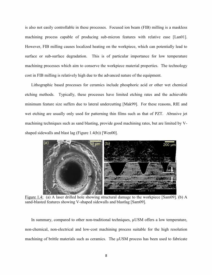
Figure 1.4: (a) A laser drilled hole showing structural damage [Sam09]. (b) A sand-blasted

features showing V-shaped sidewalls and blastlag [Sam09]…………………………….………08

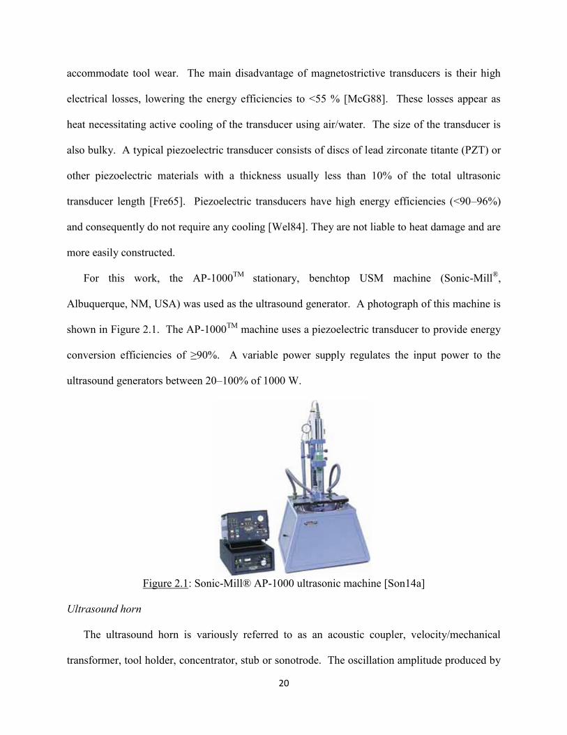
Figure 2.1: Sonic-Mill® AP-1000 ultrasonic machine [Son14a]……………………………….20

Figure 2.2: Typical horn designs: (a) Exponential (b) Rectangular (c) Cylindrical [Son14_2]

…………………………………………………………………………………………………....21

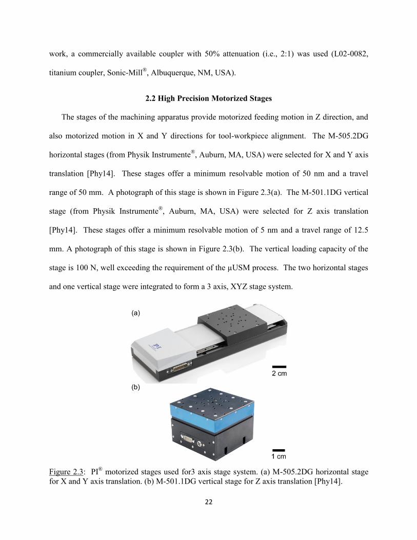
Figure 2.3: PI® motorized stages used for3 axis stage system. (a) M-505.2DG horizontal stage

for X and Y axis translation. (b) M-501.1DG vertical stage for Z axis translation

[Phy14]….......................................................................................................................................22

Figure 2.4: HD15 acoustic emission sensor with 2/4/6C preamp from Physical Acoustics

Corporation…………………………………………………………………………………...….24

Figure 2.5: Conceptual diagram of serial mode fabrication of SS304 micro-tool. (a-b) Wire

electro-discharge grinding (WEDG) of a 300-µm diameter stainless steel (SS) tool in order to

flatten the tip surface and then reduce the tool diameter. (c-d) Electro-discharge machining

(EDM) of a SS substrate to form tool carrier to hold the tool perpendicularly. (e) The tool is

inserted into the cavity of the tool carrier and bonded using STYCAST

epoxy…………...……………………………………………………………………………...…26

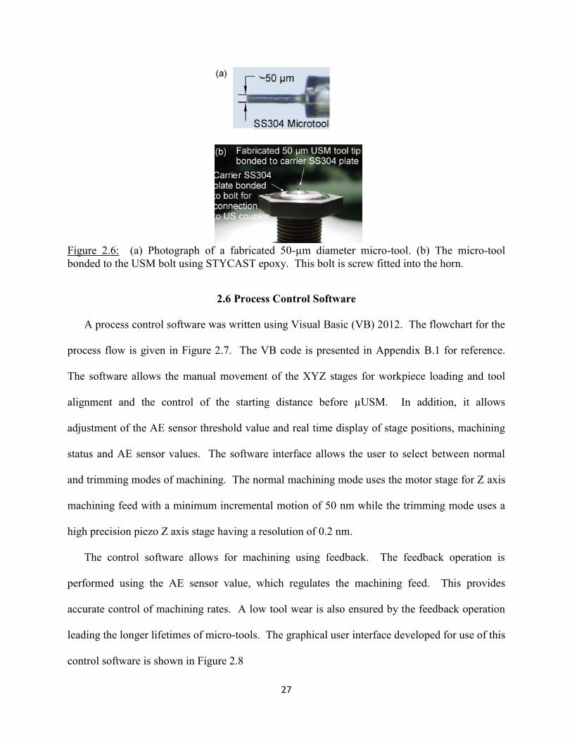
Figure 2.6: (a) Photograph of a fabricated 50-µm diameter micro-tool. (b) the micro-tool

bonded to the USM bolt using STYCAST epoxy. This bolt is screw fitted into the horn.

…………………………………………………………………………………….……………...27

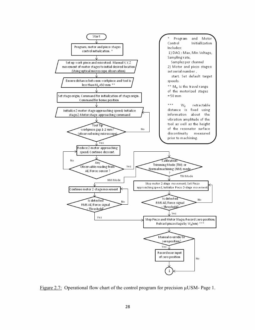
Figure 2.7: Operational flow chart of the control program for precision µUSM…………...28/29

Figure 2.8: Graphical user interface of control program for precision machining. ...…………..30

ix

Figure 2.9: (a) Customized aluminum mounting fixture for integration of motorized stages onto

the USM platform (b) Customized aluminum worktable to hold workpiece during µUSM.

……………………………………………………………………………………………….…...31

Figure 2.10: Photograph of the customized µUSM system showing various components.

………………………………………………………………………………………………...….32

Figure 3.1: Conceptual comparison of micro ultrasonic machining (µUSM) used for

conventional µUSM and for HR-µUSM. (a) Conventional µUSM produces deeper machined

features with rougher surfaces. (b) HR-µUSM uses greater, fixed, distances between tool and

workpiece, smaller abrasive particles and lower tool vibration amplitude. ……………………..35

Figure 3.2: Dependence of machining rate on abrasive particle size and tool vibration amplitude

based on equation (1). The use of ≈10 nm abrasive particle sizes and <1 µm tool vibration

amplitude theoretically allows machining rates of approximately 5-15 µm/min (80-250 nm/sec).

………………………………………………………………………………………………...… 36

Figure 3.3: Results of FEA analysis showing slurry flow patterns during HR-µUSM of different

workpiece profiles (a) Vortex slurry flow pattern seen on a flat surface. The maximum slurry

velocity observed on a flat fused silica substrate is 0.24 m/s. (b) Slurry flow pattern for a curved

profile of 30-µm depth. Maximum fluid velocity observed on curved surface is negligible.

…………………………………………………………..………………………………………..38

Figure 3.4: (a) Machining depth as a function of machining time (b) Machining rate as a

function of machining time. Machining rate averaged ≈100 nm/sec at the end of the window.

…………………………………………………………………………………………………....40

Figure 3.5: Average surface roughness, Sa, as a function of machining time. The minimum Sa

observed was 30 nm; this was obtained with 10 nm diamond powder in 3 minutes. ………...…41

Figure 3.6: SEM images of machined features using: (a) Tungsten Carbide (1 µm,

WC:H2O=1:1 by wt.). The machined feature diameter was 73 µm. The corresponding average

surface roughness, Sa, was 245 nm. (b) Tungsten Carbide (100 nm). The machined feature

diameter was 69 µm. The corresponding Sa was 67 nm. (c) Diamond (10 nm) slurry. The

machined feature diameter was 75 µm. The corresponding Sa was 30 nm. Each machining was

performed for 2 minutes. (d) A typical profile of the machined feature using diamond (10 nm)

slurry. Measured values of Sa at locations 1-6 denoted in (c) are provided in Table 3.2. …...…42

Figure 3.7: (a) A birdbath (BB) hemispherical shell of 5-mm diameter [6]. The inset shows a

BB shell and the microtool after machining. (b-d) Results of trimming of BB shells using HR-

µUSM. (b) Trimming of the top surface of the shell rim. Average machining rate measured was

102 nm/sec. (c) Trimming of the outer sidewall of shell. Average machining rate measured was

84 nm/sec. (d) Trimming of the bottom surface of the shell. Average machining rate measured

was 60 nm/sec. ………………………………………………………………………..…………44

Figure 3.8: Modifications to tool/mounting configurations for trimming of BB shells. (a)

Configuration A for shell rim and sidewall trimming: use of shorter tool lengths (2–5 mm) and

adhesive layers around the shell for mechanical support. (b) Configuration B for shell bottom

trimming: use of longer tools (5–10 mm) and slurry localized within the shell. ………………..46

x

Figure 4.1: Concept of batch-mode μUSM using workpiece vibration. The batch-tool is static

while the workpiece vibrates in the cutting direction. A gradual feed of the workpiece towards

the tool causes machining due to physical attrition of the abrasive particles on the workpiece.

……………………………………………………...…………………………………………....50

Figure 4.2: P.885.51 PICMA® multilayer stack actuator [Phy14]. ............…………………….52

Figure 4.3: Schematic of setup used to measure vibration amplitude of the workpiece………..54

Figure 4.4: Vibration amplitude of the workpiece as a function of PZT actuation voltage. The

PZT was loaded with 25 g weight comprising of glass slide, workpiece, clay reservoir and slurry.

……………………………………………………………………………………………………55

Figure 4.5: Machining depth and rate dependence on transducer actuation voltage. …….…….56

Figure 4.6: Surface roughness, Sa, dependence on PZT actuation voltage. …………………….57

Figure 4.7: Machined depth dependence on machining time- with and without feeding. ……..57

Figure 4.8: Stainless steel micro-tool array design- perspective view. …………………..…….58

Figure 4.9: Stainless steel micro-tool array design- dimensions. ………………………..……..58

Figure 4.10: Results of FEA analysis showing slurry flow patterns during batch-mode µUSM

using workpiece vibration (a) Uniform slurry flow pattern seen due to vibration of workpiece

surface. (b) Slurry velocity magnitude at micro-tool array: ≈2.46 m/s at the surfaces of the tool

tips and ≈0.13 m/s at the surface of the tool substrate. Slurry velocity magnitude at workpiece

surface: ≈2.37 m/s at the target machining locations and ≈0.64 m/s away from cutting zones.

……………………………………………………………………………………………………60

Figure 4.11: Photograph of a fabricated 2×3 stainless steel micro-tool array (unreleased). The

tools have a height of 300 µm and a lateral feature size of 50 µm. ……………………………..61

Figure 4.12: SEM image of a fabricated 5×5 stainless steel micro-tool array (unreleased). The

tools have a height of 40 µm and a lateral feature size of 5 µm……………………………...….62


tools have a height of 50 µm and a lateral feature size of 12 µm, with an improved tool geometry

compared to 5 µm tools………………………………………………………………………….62

Figure 4.14: Machined depth dependence on transducer actuation voltage. The machined depth

represents the average of the depth of all micro-tool array elements machined on the workpiece.

……………………………………………………………64

Figure 4.15: Surface roughness, Sa, dependence on transducer actuation voltage. The surface

roughness represents the average of the Sa of all micro-tool array elements machined on the

workpiece. ……………………………………………………………………………………….64

Figure 4.16: SEM image of a 50-µm lateral size features machined using the micro-tool array

fabricated using serial-mode µEDM. The inset shows a close up of one of the features. ………65

xi

Figure 4.17: The variation in machined depth across different elements in an array. The

variation in depth is less than ±3 % ……………………………………………………………..65

Figure 4.18 The variation in surface roughness, Sa, across different elements in an array. The

variation in Sa is less than ±20 % ………………………………………………………………..65

Figure 4.19: Dependence of silicon tool wear rate on abrasive particle size and tool vibration

amplitude based on equation (1). Theoretically, use of ≈100 nm abrasive particle sizes and 2.5

µm tool vibration amplitude causes tool wear rates approximately 14 µm/min (≈230 nm/sec).

…………………………………………………………………………………………………....67

Figure 4.20: Process flow for the fabrication of micro-tools using DRIE of silicon. ……….….68

Figure 4.21: SEM images of micro-tools fabricated using DRIE. (a) Micro-tool pattern of 2-µm

feature size. The inset shows a closeup of the features. (b) Micro-tool pattern of 5-µm feature

size. The inset shows a closeup of the features. (c) Micro-tool pattern of 1-µm feature size. (d)

Micro-tool pattern of 40 µm circular spirals. The average height of all tools is ≈20 µm.

…………………………………………………………………………………………..………..69

Figure 4.22: Optical and SEM images of cross patterns transferred to a fused silica substrate

using 5-µm lateral size tools. (a) SEM image of the patterns. (b) 3-D view of height intensities

obtained using interferometry. (c) Optical image of the top view (focused on the top FS surface).

(d) Optical image of the top view (focused on the bottom trench surface). The features have an

average lateral size of 8 µm, depth of 6 µm and a surface roughness, Sa of 23 nm. The aspect

ratio of resulting machined features was ≈3:4 …………………………………………………..71




(d) Optical image of the top view (focused on the bottom trench surface). The features have an

average lateral size of 4 µm, depth of 2.7 µm and a surface roughness, Sa of 12 nm. The aspect

ratio of resulting machined features was ≈2.7:4…………………………………………………72

Figure A.1: Sensor and stent geometry showing important dimensions. A sensor bonded to a

single stent cell is also shown……………………………………………………………………81

Figure A.2: Process flow for the fabrication of bi-layer stent cell resonators integrated with the

stent. (1) MetglasTM

2826MB and Elgiloy foils are aligned and bonded using the Au-In eutectic

bonding process to form the bi-layer. (2) Batch patterning of the bonded foils is performed using

µ-EDM. (3) Bi-layer stent cell resonators at specific locations along the stent frame are

fabricated. Parylene deposition is then performed on the resonators to passivate them and make

them bio-compatible……………………………………………………………………………..82

Figure A.3: Fabricated resonators using µEDM (a) Isolated sensor comprising of bi-layer

MetglasTM

-Elgiloy resonators. (b) Perspective view of the anchor of the bi-layer resonators.

……………………………………………………………………………………………………83

Figure A.4: Frequency response of unloaded sensor in air. The measured resonant frequency is

361 kHz while the custom magnetomechanical FEA model resonates at 346 kHz……...………84

xii

Figure A.5: Measured resonance plots of bi-layer resonators in flow at 37°C. Diastolic (flow

velocity of 20 cm/sec) observed fres=356.5 kHz while systolic (flow velocity of 11cm/sec)

observed fres=356.6 kHz………………………………………………………………………….84

Figure A.6: Stent cell resonator response to changes in viscosity levels. Viscosity is varied from

1.1 cP to 15.4 cP using varying concentrations of sugar (sucrose) in water. The resonant

frequencies measured are normalized to the unloaded, sensor resonant frequency in air…….…85

Figure A.7: Stent cell resonator response to mass loading in water flow (velocity of 15 cm/sec)

and at a temperature of 37°C. Mass loading is provided by paraffin wax. Mo denotes the

unloaded sensor mass and ∆m the mass load on the sensor……………………………..………85

Figure B.1: Design of aluminum mounting fixture……………………………………………110

Figure B.2: Design of aluminum worktable………………………………………………...…111

xiii

LIST OF TABLES

Table 1.1: Capabilities of common NLB micromachining technologies compared with that of

high precision µUSM (this work)……………………………………………………………..…12

Table 2.1: Comparison of conventional µUSM system parameters with that of the customized

system for precision µUSM……………………………………………………………………...32

Table 3.1: Machining rate as a function of fixed distance (FD) averaged over 1 min. 100 nm

WC particles was used in the slurry…………………………………………………………...…39

Table 3.2: Average surface roughness (Sa) measured at six different areas of a feature machined

with 10 nm diamond slurry powder (Figure 3.6(c)). …………………………………….…...…43

Table 3.3: Machining results for HR-µUSM…………………………………………….…..…43

Table 4.1: Relevant device specifications of the P.885.51 PICMA® multilayer stack actuator

……………………………………………………………………………………………..…..…52

Table 4.2: Machining parameters used for characterization of machining rate, MR, and surface

roughness, Sa, on workpiece vibration amplitude. ………………………………..………..……55

Table 4.3: Machining parameters used in characterization of MR and surface roughness, Sa, on

machining time- with and without tool feeding. ………………………………………….…..…57

Table 4.4: Machining parameters used in demonstration of batch-mode µUSM using micro-tool

array fabricated by serial µEDMTable 4.5: Typical machining parameters used for batch pattern

transfer from DRIE silicon micro-tools. …………………………………………………..…….63

Table 4.5: Typical machining parameters used for batch pattern transfer from DRIE silicon

micro-tools………………………………………………………………………………….……71

xiv

LIST OF APPENDICES

APPENDIX A: Metglas- Elgiloy magnetoelastic sensors fabricated using µEDM…………..…80

APPENDIX B: Program Script of Process Control Software for the Precision μUSM Apparatus;

Engineering drawings of the customized aluminum worktable and mounting fixture..................87

APPENDIX C: Fabrication Process Flow of the DRIE Silicon Micro-Tools for µUSM……... 112

APPENDIX D: List of Publications Related to This Dissertation…………………………...…114

xv

ABSTRACT

Micro ultrasonic machining, µUSM, is a non-thermal, nonchemical and non-electrical

process that is especially suitable for hard, brittle, and inert insulators such as ceramics.

Typically, the µUSM process is capable of machining rates ≥300nm/sec; the resulting surface

roughness is Sa≥250nm. There is a compelling need to extend this micromachining approach in

precision and resolution for a variety of MEMS, such as for the high resolution trimming of

timing references. However, a number of challenges must be addressed including the

development of appropriate equipment, methodology of tool design and fabrication, and

optimization of machining parameters.

The research described in this thesis addresses the challenges for high resolution micro

ultrasonic machining (HR-µUSM), providing high resolution and high surface quality, and

precise control of machining rates. Experimental results demonstrate that the HR-µUSM process

achieves machining rates as low as 10nm/sec averaged over the first minute of machining of

fused silica substrates. This corresponds to a mass removal rate of ≈20ng/min. The average

surface roughness, Sa, achieved is as low as 30nm, which is an order of magnitude lower than

conventional µUSM. The process is used to demonstrate trimming of hemispherical 3-D shells

made of fused silica.

Additionally, this thesis addresses a challenge of slurry precipitation or settling during 3-D

machining using µUSM, which drastically reduces the machining rates to negligible values. A

mode of μUSM is developed in which the workpiece is vibrated and not the tool. Experimental

xvi

evaluations of this process result in machining rates ranging typically from 5–50 nm/sec for

vibration levels ranging from 1–8 μm. The workpiece vibration agitated the abrasive particles,

alleviating slurry settling.

Finally, this thesis explores the resolution limit of µUSM using lithographically patterned

silicon micromachined tools. The use of lithography enables the batch mode transfer of complex

patterns, greatly enhancing the throughput of the process. Silicon microstructures with high

resolution(≤10 µm) and high aspect ratio(≥20:1) can be readily made using deep reactive ion

etching (DRIE). Fine featured Si cutting tools are lithographically patterned and fabricated.

Machining evaluations result in the successful transfer of patterns with sub-10 μm feature sizes

and ≈3:4 aspect ratios.

1

Chapter 1

Introduction

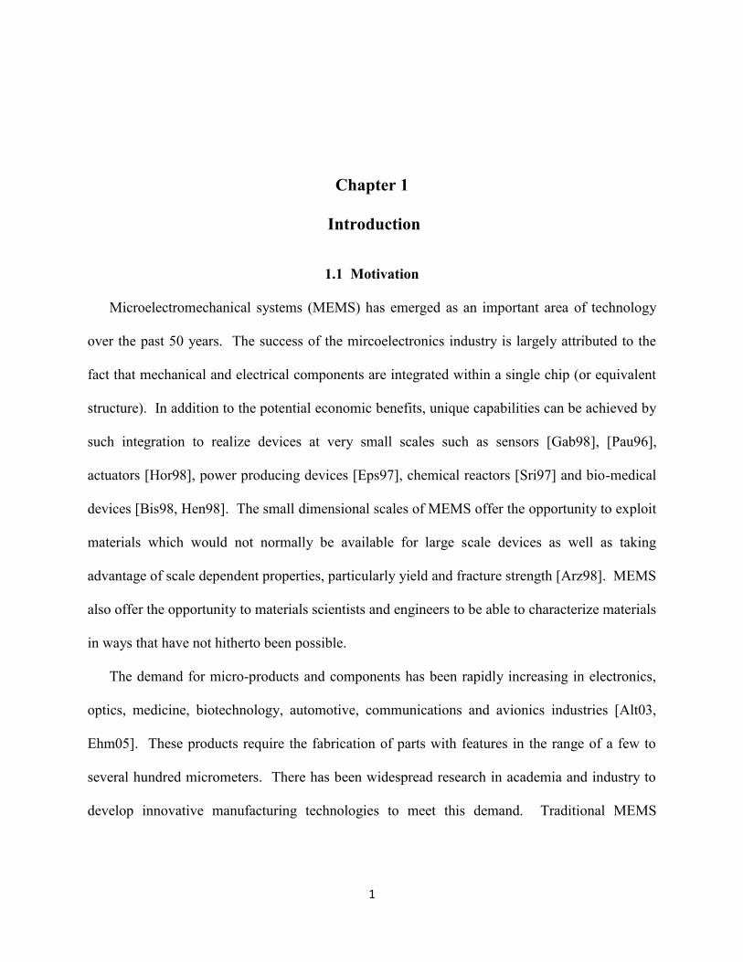
1.1 Motivation

Microelectromechanical systems (MEMS) has emerged as an important area of technology

over the past 50 years. The success of the mircoelectronics industry is largely attributed to the

fact that mechanical and electrical components are integrated within a single chip (or equivalent

structure). In addition to the potential economic benefits, unique capabilities can be achieved by

such integration to realize devices at very small scales such as sensors [Gab98], [Pau96],

actuators [Hor98], power producing devices [Eps97], chemical reactors [Sri97] and bio-medical

devices [Bis98, Hen98]. The small dimensional scales of MEMS offer the opportunity to exploit

materials which would not normally be available for large scale devices as well as taking

advantage of scale dependent properties, particularly yield and fracture strength [Arz98]. MEMS

also offer the opportunity to materials scientists and engineers to be able to characterize materials

in ways that have not hitherto been possible.

The demand for micro-products and components has been rapidly increasing in electronics,

optics, medicine, biotechnology, automotive, communications and avionics industries [Alt03,

Ehm05]. These products require the fabrication of parts with features in the range of a few to

several hundred micrometers. There has been widespread research in academia and industry to

develop innovative manufacturing technologies to meet this demand. Traditional MEMS

2

fabrication technologies are capable of producing micro or sub-micrometer size features.

However these techniques do have limitations such as restricted choice of work materials,

inability to produce complex geometries, huge capital investment and inevitable cleanroom

environment [Liu04]. Non-traditional fabrication technologies are not widely commercialized

due to their immature status as reliable mass production methods [Ehm05]. However they do

provide new ways in subtractive and additive processes to overcome limitations (of MEMS) in

geometry and materials. Non-traditional processes also offer economical solutions for the

micromachining of small and medium quantities.

Ceramics in MEMS

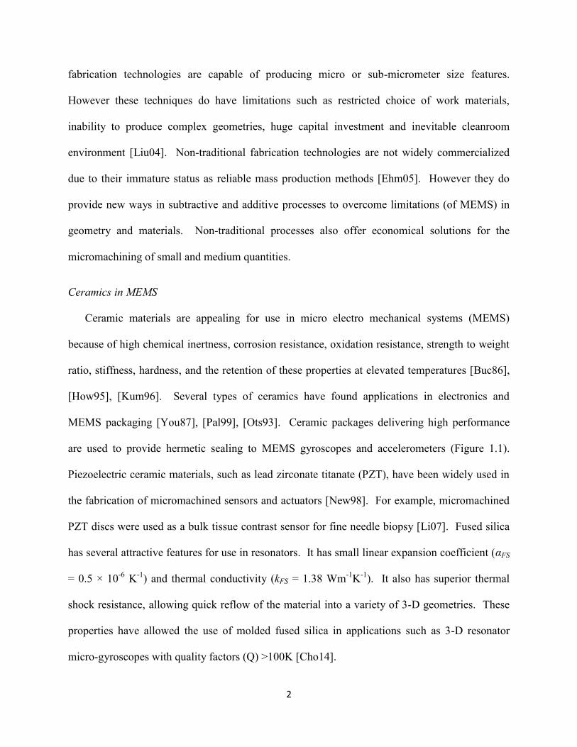
Ceramic materials are appealing for use in micro electro mechanical systems (MEMS)

because of high chemical inertness, corrosion resistance, oxidation resistance, strength to weight

ratio, stiffness, hardness, and the retention of these properties at elevated temperatures [Buc86],

[How95], [Kum96]. Several types of ceramics have found applications in electronics and

MEMS packaging [You87], [Pal99], [Ots93]. Ceramic packages delivering high performance

are used to provide hermetic sealing to MEMS gyroscopes and accelerometers (Figure 1.1).

Piezoelectric ceramic materials, such as lead zirconate titanate (PZT), have been widely used in

the fabrication of micromachined sensors and actuators [New98]. For example, micromachined

PZT discs were used as a bulk tissue contrast sensor for fine needle biopsy [Li07]. Fused silica

has several attractive features for use in resonators. It has small linear expansion coefficient (αFS

= 0.5 × 10-6

K-1

) and thermal conductivity (kFS = 1.38 Wm-1

K-1

). It also has superior thermal

shock resistance, allowing quick reflow of the material into a variety of 3-D geometries. These

properties have allowed the use of molded fused silica in applications such as 3-D resonator

micro-gyroscopes with quality factors (Q) >100K [Cho14].

3

Figure 1.1: High performance ceramics packages for accelerometers and gyroscopes (from

Analog Devices® and Colibrys

®).

A variety of non-traditional processes have been researched on for the fabrication of three

dimensional MEMS components from ceramics. Rather than covering the entire range of these

processes, this work focuses on one micromachining processes: micro ultrasonic machining

(µUSM), which is an indispensable sub-set of the non-traditional technologies.

1.2 Non-Traditional Micromachining Technologies in MEMS

Non-traditional technologies offer capabilities for the fabrication of 3-D strcutures from

broader range of materials. This is an intrinsic limitation of traditional technologies, such as the

surface and bulk micromachining of silicon. Examples of non-traditional technologies include

µUSM, micro electrodischarge machining (µEDM), laser machining, and abrasive jet machining.

1.2.1 The µUSM process

The µUSM process is a non-thermal, non-chemical and non-electrical micromachining

process that is especially suitable for hard, brittle materials such as glass, ceramics, quartz,

precious stones, and graphite. Unlike µEDM, µUSM does not depend on the electrical

properties of the workpiece. In conventional µUSM, high frequency electrical energy is

converted into mechanical vibrations [Mor88], [Far80], which causes a tool to vibrate along its

longitudinal axis at high frequency (usually at 20–40 kHz) with an amplitude of 10–50 µm

[Bal64], [Cli93]. An abrasive slurry (comprising a mixture of abrasive material, e.g. silicon

4

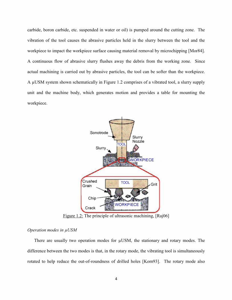
carbide, boron carbide, etc. suspended in water or oil) is pumped around the cutting zone. The

vibration of the tool causes the abrasive particles held in the slurry between the tool and the

workpiece to impact the workpiece surface causing material removal by microchipping [Mor84].

A continuous flow of abrasive slurry flushes away the debris from the working zone. Since

actual machining is carried out by abrasive particles, the tool can be softer than the workpiece.

A µUSM system shown schematically in Figure 1.2 comprises of a vibrated tool, a slurry supply

unit and the machine body, which generates motion and provides a table for mounting the

workpiece.

Figure 1.2: The principle of ultrasonic machining, [Raj06]

Operation modes in µUSM

There are usually two operation modes for µUSM, the stationary and rotary modes. The

difference between the two modes is that, in the rotary mode, the vibrating tool is simultaneously

rotated to help reduce the out-of-roundness of drilled holes [Kom93]. The rotary mode also

5

reduces machining load and extends tool life. Because of the rotary motion, the rotary mode can

only be used for circular-hole drilling in most situations, and is not applicable for batch mode

pattern transfer.

Capabilites of µUSM

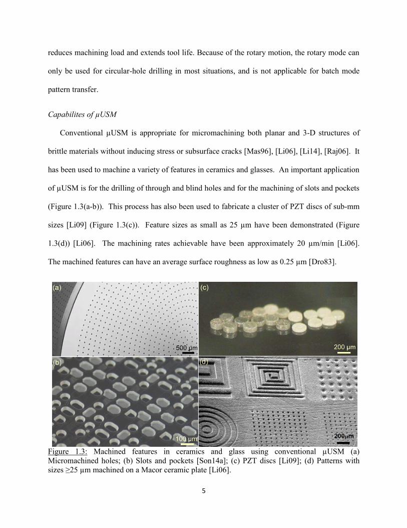
Conventional µUSM is appropriate for micromachining both planar and 3-D structures of

brittle materials without inducing stress or subsurface cracks [Mas96], [Li06], [Li14], [Raj06]. It

has been used to machine a variety of features in ceramics and glasses. An important application

of µUSM is for the drilling of through and blind holes and for the machining of slots and pockets

(Figure 1.3(a-b)). This process has also been used to fabricate a cluster of PZT discs of sub-mm

sizes [Li09] (Figure 1.3(c)). Feature sizes as small as 25 µm have been demonstrated (Figure

1.3(d)) [Li06]. The machining rates achievable have been approximately 20 µm/min [Li06].

The machined features can have an average surface roughness as low as 0.25 µm [Dro83].

Figure 1.3: Machined features in ceramics and glass using conventional µUSM (a)

Micromachined holes; (b) Slots and pockets [Son14a]; (c) PZT discs [Li09]; (d) Patterns with

sizes ≥25 µm machined on a Macor ceramic plate [Li06].

6

The µUSM process, which was initially considered as a complementary technique to

lithographic processes, has matured to offer true three-dimensional machining capability to

process a wide variety of engineering materials including ceramics and polymers. However the

use of this process for fine resolution and precision machining of substrates has not been

explored in detail.

1.2.2 The µEDM process

The µEDM process is the successful adaptation of EDM for micromachining features that

range from simple holes to complex molds [Tak02]. Here the discharge energy is reduced to the

order of 10-6

to 10-7

Joules in order to minimize the unit material removal per discharge. Electro-

discharge machining is based on the erosion of the material to be machined by means of a

controlled electric discharge between an electrode and the material. The gap phenomena include

plasma formation in the dielectric, interaction between electrons and ions, heat transfer and

material ejection. The µEDM process, ofcourse, requires the substrate to be conductive or semi-

conductive. The µEDM process has been mainly used to machine a variety of metals and semi-

conductors and is not suitable for ceramic machining.

Based on the electrode being used, µEDM can be classified into drilling, die-sinking, milling,

wire EDM (WEDM) and wire electro-discharge grinding (WEDG) [Mas01]. The minimum

feature sizes capable by µEDM range from 3 to 30 µm depending on the µEDM process being

used. The aspect ratios achievable using µEDM drilling and milling can be as high as 25.

Surface roughness (Ra) as low as 50 nm have been reported [Raj06]. Currently wire electro-

discharge grinding (WEDG) is the widely accepted and commercialized method to fabricate

micro tools [Mas85]. Using single pulse discharge is an innovative technique to produce 20~40

μm diameter tungsten electrodes in hundreds of microseconds. While tungsten tool electrodes

7

are attractive for µEDM, WEDG can be used to fabricate micro-tools from other materials such

as stainless steel which are more preferable for µUSM for its tool wear properties. These tools

can then be used in µUSM to achieve very fine feature sizes.

µEDM has been widely used for the fabrication of 3-D structures with feature sizes ≥5 µm.

Serial and batch manufacturing of cardiac stents has been demonstrated in [Tak04], [Tak06].

While the fabrication of structures with complex shapes and small features sizes using µEDM

has been demonstrated before, the integration of these structures to form a sensor/actuator faces

certain challenges. Some of these challenges are explored in Appendix A. Specifically,

Metglas-Elgiloy stent cell resonators are fabricated using µEDM and their application to

viscosity and mass sensing is investigated [Vis13].

1.2.3 Other non-traditional technologies for ceramic machining

In the macro scale, ceramics (including PZT) are often processed by molding from a powder

form. Some examples of these processes include dry pressing or tape casting, fused deposition

(FDC) and sol gel process. However these additive processes suffer from problems which are

especially significant in the micro-scale. Among these, volume shrinkage, high temperature

steps, non-uniform material properties and difficulty in mold forming are predominant [Li06].

Thus, it is often desirable to directly pattern a bulk material without degrading the original

material properties. Subtractive processes are favorable in this regard. However, subtractive

processes have their own challenges.

Among serial subtractive processes, laser drilling and diamond grinding are commonly used

for precision machining of ceramics. However these processes are unfavorable for transfer of

complex patterns which can be best defined by a mask. Laser drilling has also been known to

causes thermal shock and changes in morphology (Figure 1.4(a)). The mass removal rate (MRR)

8

is also not easily controllable in these processes. Focused ion beam (FIB) milling is a maskless

machining process capable of producing sub-micron features with relative ease [Lan01].

However, FIB milling causes localized heating on the workpiece, which can potentially lead to

surface or sub-surface degradation. This is of particular importance for low temperature

machining processes which aim to conserve the workpiece material properties. The technology

cost in FIB milling is relatively high due to the advanced nature of the equipment.

Lithographic based processes for ceramics include phosphoric acid or other wet chemical

etching methods. Typically, these processes have limited etching rates and the achievable

minimum feature size suffers due to lateral undercutting [Mak99]. For these reasons, RIE and

wet etching are usually only used for patterning thin films such as that of PZT. Abrasive jet

machining techniques such as sand blasting, provide good machining rates, but are limited by V-

shaped sidewalls and blast lag (Figure 1.4(b)) [Wen00].

Figure 1.4: (a) A laser drilled hole showing structural damage to the workpiece [Sam09]. (b) A

sand-blasted features showing V-shaped sidewalls and blastlag [Sam09].

In summary, compared to other non-traditional techniques, µUSM offers a low temperature,

non-chemical, non-electrical and low-cost machining process suitable for the high resolution

machining of brittle materials such as ceramics. The µUSM process has been used to fabricate

9

intricate features in ceramics with sizes ≥25 µm and roughness, Sa≥ 0.25 µm, without causing

any surface or sub-surface degradation to the workpiece. However, the use of this process for

fine resolution and precision machining faces several challenges, which have been explored in

detail in this work.

1.3 Micro USM: Serial Mode or Batch Mode

Serial mode µUSM

In conventional µUSM the tool is usually attached to the horn by either soldering or brazing,

screw/taper fitting. Alternatively, the actual tool configuration can be machined on to the end of

the horn. In the micron domain (<100 µm), problems associated with the mounting accuracy and

the fabrication of micro-tools arise. To solve these problems, wire electrode discharge grinding

(WEDG) has been used to machine micro-tools with diameters ≤25 µm. Serial mode µUSM has

been demonstrated in microscale and feature size as small as 5μm in glass and silicon has been

achieved [Ega99], showing excellent potential for MEMS applications. These serial mode

subtractive processes have been commonly used for conventional precision machining of

ceramics and have their own advantages depending on the application situations, while they also

have their own limitations. Importantly, serial processes are usually limited by the inherently

low throughput. For example, the micro-tool shaped by WEDG is mainly favorable for the

drilling of microholes. More complex patterns such as slots and levers can be realized by using a

simple “pencil” tool and contour machining the complex shape with a CNC program. Recently,

the feasibility of using this technique has become of interest and has been investigated in a

number of countries including the UK, France, Switzerland, Japan, etc. [Nis56], [Tho94]. A few

CNC controlled path rotary USM systems are available commercially such as the SoneX 300

(Extrude Hone Limited, France) and the Erosonic US400/US800 (Erosonic AG, Switzerland).

10

However, this approach not only largely reduces the throughput of the process, especially for

complex patterns, but also limits the structural shapes the process can handle [Nis54].

Batch mode µUSM

A batch mode operation in μUSM greatly enhances the throughput of the process and

provides the ability to transfer complex patterns onto ceramic substrates. The fabrication of

batch tools in µUSM can be non-lithographically based (NLB) as well as lithographically based

(LB). Processes such as μEDM can be used to fabricate micro-tool arrays for USM with feature

sizes ≥5 µm [Raj06], [Li06], [Li14]. Serial micro EDM can be used to transfer simple tool

patterns with relative ease onto stainless steel substrates [Li06]. This process is suitable for rapid

prototyping of machining processes.

In order to truly improve the throughput and the ability to machine complex patterns, it is

desired to fabricate micro-tools lithographically. If the μUSM process can be combined with

lithography and have the pattern transferred in die-scale or even waferscale, not only is the

machining throughput greatly improved, but the easy integration with other micromachining

steps and familiar approach for pattern definition and customization will enhance its usability in

many potential MEMS applications. The batch mode μEDM process can be applied to make the

micro-tool for batch mode μUSM, which can facilitate die-scale transfer of complex lithographic

patterns to ceramics with potentially high resolution and throughput, while retaining the favored

characteristics of conventional USM.

Lithography based techniques for fabricating micro-tools have been explored in the past. A

process (named LEEDUS: a combination of lithography, electroplating, μEDM and μUSM)

allowing batch-mode pattern transfer onto ceramic dies was described in [Li06], [Li09]. In this

process, an electroplating mold is first created on a silicon or metal wafer using standard

11

lithography, then using the electroplated pattern as an electrode to EDM a hard metal (stainless

steel or WC/Co) tool, which is finally used in the USM of the ceramic substrate. The machining

rates achieved in that work were ≥18 μm/min. The corresponding surface finish, Ra, of

machined features ranged from 0.4–0.7 μm.

1.4 Precision and Scalability in µUSM

Unlike conventional µUSM, the application of precision and high resolution µUSM for very

fine machining of ceramics is of interest to a number of MEMS industries. In particular, it is

appealing for the post-fabrication trimming of inertial sensors, timing references and mass-

balance resonators to adjust stiffness, mass and potentially damping [Kem11], [Pue12]. While

the resolution of machining and feature sizes depend on the tool sizes used during machining, the

material removal rate is determined mainly by the impact velocity which is a function of the

frequency and the amplitude of the vibrating tool as well as the distance between the tool and the

workpiece. The surface finish depends on the particle size of the abrasive used in the ultrasonic

machining.

Abrasive particle size, vibration amplitude, tool proximity and slurry behavior are the main

parameters influencing the micro USM machining speed for the given workpiece material

[Hu05]. At present the proper selection of these process parameters required for precision

machining is not well understood due to lack of experimental results. Consequently, µUSM has

not yet been commercialized as a functional machine tool at a scale similar to µEDM. However,

it is believed that this process could provide solutions to easily and quickly achieve the larger

MEMS structures as well as packaging for both prototype and production in silicon, glass and

ceramic [Med05]. This is worthy of future research.

12

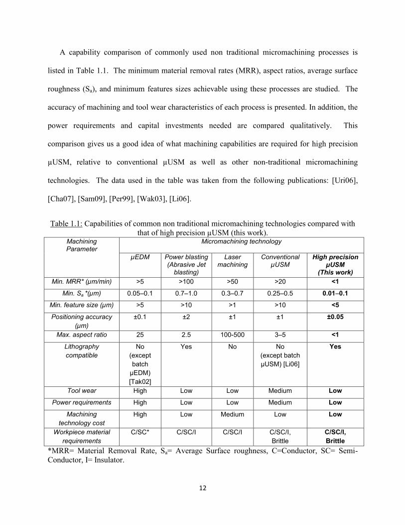
A capability comparison of commonly used non traditional micromachining processes is

listed in Table 1.1. The minimum material removal rates (MRR), aspect ratios, average surface

roughness (Sa), and minimum features sizes achievable using these processes are studied. The

accuracy of machining and tool wear characteristics of each process is presented. In addition, the

power requirements and capital investments needed are compared qualitatively. This

comparison gives us a good idea of what machining capabilities are required for high precision

µUSM, relative to conventional µUSM as well as other non-traditional micromachining

technologies. The data used in the table was taken from the following publications: [Uri06],

[Cha07], [Sam09], [Per99], [Wak03], [Li06].

Table 1.1: Capabilities of common non traditional micromachining technologies compared with

that of high precision µUSM (this work). Machining Parameter

Micromachining technology

µEDM Power blasting (Abrasive Jet

blasting)

Laser machining

Conventional µUSM

High precision µUSM

(This work)

Min. MRR* (µm/min) >5 >100 >50 >20 <1

Min. Sa *(µm) 0.05‒0.1 0.7‒1.0 0.3‒0.7 0.25‒0.5 0.01‒0.1

Min. feature size (µm) >5 >10 >1 >10 <5

Positioning accuracy

(µm)

±0.1 ±2 ±1 ±1 ±0.05

Max. aspect ratio 25 2.5 100-500 3‒5 <1

Lithography

compatible

No

(except

batch

µEDM)

[Tak02]

Yes No No

(except batch

µUSM) [Li06]

Yes

Tool wear High Low Low Medium Low

Power requirements High Low Low Medium Low

Machining

technology cost

High Low Medium Low Low

Workpiece material

requirements

C/SC* C/SC/I C/SC/I C/SC/I,

Brittle

C/SC/I,

Brittle

*MRR= Material Removal Rate, Sa= Average Surface roughness, C=Conductor, SC= Semi-

Conductor, I= Insulator.

13

As seen in Table 1.1, the high precision µUSM process in this work aims to achieve low

material removal rates, smooth surfaces and small feature sizes. Low material removal rates (<1

µm/min or <16 nm/sec) can provide improved control of machining in the vertical (depth)

direction. Superior surface finishes (surface roughness, Sa of 10–100 nm) are targeted. The

process also targets to achieve minimum features sizes of <5 µm, pushing the limits of the

conventional µUSM process. It is also desired to provide lithography compatibility to the µUSM

process to greatly enhance the machining throughput.

1.5 Goals and Challenges

Three primary goals are explored in this effort. The first goal is to develop a fabrication

technology for ultra-high precision machining of hard and brittle materials such as ceramics.

The technology is intended to provide low machining rates, high resolution and high surface

quality, unlike conventional μUSM. The second goal is to explore a mode of μUSM in which

the workpiece is vibrated and not the tool. The main motivation behind vibrating the workpiece

is to eliminate the settling of slurry particles, which presents a challenge for the machining of 3-

D microstructures. The third goal is to explore the resolution limits of μUSM using

lithographically patterned silicon micormachined tools. Silicon microstructures with high

resolution (≤10 μm) and high aspect ratios (≥20:1) can be readily made using deep reactive ion

etching (DRIE). This would allow the possibility of using fine featured cutting tools and would

greatly enhance the throughput of the μUSM process, as well as push the scalability of the

machined features to sub-10 μm levels.

The primary goals lead to five specific goals. (a) Quantitative evaluation of the impact of

particle size, slurry behavior, tool position and tool amplitude on machining rate and surface

roughness. (b) Identification and evaluation of suitable instrumentation to allow high precision

14

machining. (c) Evaluation of the ability to trim fused silica microstructures through precision

µUSM. (d) Investigation of high precision µUSM by vibratory actuation of the workpiece.

Workpiece vibration eliminates slurry precipitation or settling that presents a challenge for 3-D

machining. (e) Investigation of silicon microstructures as cutting tools for batch mode μUSM.

A set of tasks arise in order to achieve the goals listed above. The vibration amplitude,

abrasive particle sizes and tool geometry are some of the key parameters that determine the MRR

rate of a µUSM system. Numerical modeling of the µUSM process will help us understand the

effect of these parameters on MRR, surface characteristics, aspect ratios and tool wear

characteristics. This serves as a foundation for setting the machining parameters required for

high resolution machining. A finite element model of the µUSM process is needed to study

slurry flow patterns and record expected slurry flow velocities. These fluidic simulations will

also help in visualizing the machined profile after µUSM.

Once the process parameters have been studied and identified, the next goal is to identify,

develop and characterize suitable µUSM instrumentations to allow precision machining. The

customization of a conventional µUSM system involves several tasks. Conventional systems are

tailored for high mass removal rates required for industrial purposes. In order to achieve high

resolution machining, the inherent specifications of the USM machine have to be adjusted. The

USM system would have to be integrated with automated stages to provide high resolution

movement in the XYZ directions. This facilitates precise alignment of the workpiece with the

tool and low machine feeding rates for minimal mass removal. A control software is needed that

provides a user interface for precise movement of the automated stages, calibration and surface

detection, and the optimization of machining parameters. Lastly, a complete experimental

15

characterization of the customized µUSM system to study achievable machining rates and

surface roughness of machined features is needed.

In order to test the ability of the customized µUSM system, high resolution trimming of 3-D

microstructures will be performed. Minimal mass removal rates are essential to the fine mass

removal on delicate 3-D microstructures, such as on the rims of micro hemispherical resonators

to improve device symmetry.

The vibration of the workpiece in µUSM eliminates slurry precipitation or settling that

presents a challenge for 3-D machining. A complete characterization of this process provides a

basis for the setting of parameters for 3-D machining of microstructures. Specifically, the

workpiece vibration amplitude, the tool feeding, the abrasive particle sizes, and the machining

time controls the µUSM outcome in terms of machining rates and surface roughness of features.

A batch mode operation in µUSM necessitates the fabrication of micro-tool patterns with

delicate features. Non-lithographic processes, such as serial µEDM, are used to fabricate batch

tools with feature sizes ≤50 µm and aspect ratios ≥6:1. Lithographic processes such as deep

reactive ion etching (DRIE) is also explored in the fabrication of silicon cutting tools with

feature sizes ≤2 µm and aspect ratios ≥20:1. A machining evaluation using these batch tools

assesses the process efficiency in terms of machining rates, surface finishes and variations across

the batch patterns.

Several challenges are expected in order to achieve the goals set for this work. Firstly, at

present the proper selection of µUSM process parameters required for high resolution machining

is not well understood due to lack of experimental results. While an analytical study of these

parameters provides a helpful starting point, repeated experimental characterizations will be

needed to upgrade parameters to an efficient level. The repeatability of machined results must

16

also be assured. Secondly, the integration of components (automated stages, alignment

monoscope, etc.) to a conventional µUSM system requires the design and fabrication of

additional accessories such as worktables and mounting features. The choice of high precision

automated stages must be such that they meet all geometric and loading requirements of the base

µUSM system. Thirdly, the control software for machining must be designed to be versatile

enough for different machining processes. While providing various choices with respect to stage

movement and threshold voltage values, it should also be user friendly.

The high resolution trimming of the 3-D microstructures (goal (c)) poses additional

challenges that have to be dealt with. Firstly, an effective means of mounting these

microstructures onto a carrier substrate is required. Secondly, a high accuracy of alignment of

the µUSM tool tip with the target cutting region is needed for precision machining. This requires

an effective calibration procedure prior to machining for accurate loading of sample. Thirdly,

the trimming of delicate microstructures with fragile, standing, features requires modifications to

be made to the tool/workpiece mounting configuration in order to prevent the acoustic energy of

µUSM from damaging these structures. Along with providing mechanical support, the mounting

layers used in the above configurations also present a flat profile to the 3-D structures to prevent

the quick precipitation of the slurry particles away from the cutting zone.

The use of silicon micro-tools in batch mode µUSM using workpiece vibration presents

significant challenges that have to be dealt with. Firstly, silicon is an inherently brittle material

and will be attacked in USM. Suitable protective coating materials have to be identified in order

to provide ductility and hardness to silicon. Secondly, the silicon micro-tools have very small

feature sizes (≤2 µm) and large aspect ratios (≥20:1). Modifications of control program have to

17

be made to allow significantly lower machining feed rates, to prevent damage to these delicate

tools during machining.

1.6 Outline

The dissertation continues with chapter 2 which discusses the instrumentation required for

precision µUSM. This chapter details the customized system providing low vibration

amplitudes, an improved accuracy in tool-workpiece alignment, fabrication and mounting

procedures for micro-tools of diameter ≤50 µm, and a process control software facilitating open

loop and feedback machining. Chapter 3 describes the high resolution µUSM (HR-µUSM)

process which aims to provide low machining rates, high resolution and superior surface

finishes. The application of HR-µUSM for the trimming of 3-D fused silica microstructures is

presented in this chapter. Chapter 4 presents a batch mode µUSM process using workpiece

vibration and the exploration of using DRIE Si microstructures as cutting tools. The vibration of

the workpiece in µUSM eliminates slurry precipitation or settling, enabling 3-D machining. The

resolution limit of µUSM is explored by using silicon micromachined tools with sub-10 µm.

Chapter 5 presents the conclusions and future work associated with this research effort.

18

CHAPTER 2

Micro Ultrasonic Machining Instrumentation

Conventional USM systems are tailored for high mass removal rates required for industrial

purposes. To enable high resolution and precision in machining, the inherent specifications of

the USM machine have to be adjusted. The main goals of the customized system are low

vibration amplitudes, an improved accuracy in tool-workpiece alignment, fabrication and

mounting procedures for micro-tools of diameter ≤50 µm, and a process control software

facilitating open loop and feedback machining.

The main components required for this customization include an ultrasound generator and its

controller/power supply, high precision motorized XYZ stages, an acoustic emission (AE) sensor

for feedback machining, a micro-tool, the abrasive slurry, and a process control software. The

customization of the ultrasound generator components provides a low vibration amplitude of the

tool (≤ 7 µm). Low tool vibration amplitudes enable the controlled reduction of the machining

rates. Motorized stages provide high resolution movement (≤50 nm) in the XYZ directions.

This facilitates precise alignment of the workpiece with the tool and low machine feeding rates

for minimal mass removal. The micro-tools are fabricated using the WEDG function and have

diameters ≤50 µm. The control software provides a user interface for precise movement of the

stages, calibration and surface detection needed for machining, and feedback operation.

Several challenges are addressed to meet these goals. Firstly, the integration of components

(automated stages, AE sensor etc.) to a conventional USM system requires the design and

19

fabrication of additional accessories such as worktables and mounting features. Secondly, the

choice of high precision automated stages must be such that they meet all geometric and loading

requirements of the base µUSM system. Thirdly, the control software for machining must be

designed to be versatile enough for different machining processes. A calibration procedure is

also needed for high accuracy alignment of tool-workpiece with misalignment errors <1 µm.

While providing various choices with respect to stage movement and threshold voltage values,

the control software should also be user friendly.

Section 2.1 describes the ultrasound generator used for the precision µUSM system. Section

2.2 describes the high precision motorized stages integrated with the USM system. Section 2.3

presents the acoustic emission sensor for providing feedback. Section 2.4 describes the choices

of abrasive slurries for precision µUSM. Section 2.5 describes a procedure for the fabrication

and mounting of micro-tools. Section 2.6 describes the integration of the various apparatus.

2.1 Ultrasound Generator

The main components of the ultrasound generator are the transducer and the horn. The

transducer converts a high frequency electrical signal into mechanical vibrations. These

vibrations are amplified by the horn and coupled to the tool using an acoustic coupler. The

following sections present the functionality of these components in more detail.

Transducer

The transducers used in USM are either magnetostrictive [Nis54] or piezoelectric [Sha56a].

Magnetostrictive transducers have a lower quality factor (Q) which allows the vibration to be

transmitted over a wide frequency band. It allows flexibility with the design of the horn and can

20

accommodate tool wear. The main disadvantage of magnetostrictive transducers is their high

electrical losses, lowering the energy efficiencies to <55 % [McG88]. These losses appear as

heat necessitating active cooling of the transducer using air/water. The size of the transducer is

also bulky. A typical piezoelectric transducer consists of discs of lead zirconate titante (PZT) or

other piezoelectric materials with a thickness usually less than 10% of the total ultrasonic

transducer length [Fre65]. Piezoelectric transducers have high energy efficiencies (<90–96%)

and consequently do not require any cooling [Wel84]. They are not liable to heat damage and are

more easily constructed.

For this work, the AP-1000TM

stationary, benchtop USM machine (Sonic-Mill®,

Albuquerque, NM, USA) was used as the ultrasound generator. A photograph of this machine is

shown in Figure 2.1. The AP-1000TM

machine uses a piezoelectric transducer to provide energy

conversion efficiencies of ≥90%. A variable power supply regulates the input power to the

ultrasound generators between 20–100% of 1000 W.

Figure 2.1: Sonic-Mill® AP-1000 ultrasonic machine [Son14a]

Ultrasound horn

The ultrasound horn is variously referred to as an acoustic coupler, velocity/mechanical

transformer, tool holder, concentrator, stub or sonotrode. The oscillation amplitude produced by

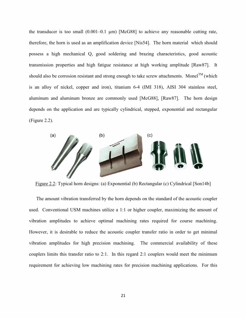
21

the transducer is too small (0.001–0.1 µm) [McG88] to achieve any reasonable cutting rate,

therefore, the horn is used as an amplification device [Nis54]. The horn material which should

possess a high mechanical Q, good soldering and brazing characteristics, good acoustic

transmission properties and high fatigue resistance at high working amplitude [Raw87]. It

should also be corrosion resistant and strong enough to take screw attachments. MonelTM

(which

is an alloy of nickel, copper and iron), titanium 6-4 (IMI 318), AISI 304 stainless steel,

aluminum and aluminum bronze are commonly used [McG88], [Raw87]. The horn design

depends on the application and are typically cylindrical, stepped, exponential and rectangular

(Figure 2.2).

Figure 2.2: Typical horn designs: (a) Exponential (b) Rectangular (c) Cylindrical [Son14b]

The amount vibration transferred by the horn depends on the standard of the acoustic coupler

used. Conventional USM machines utilize a 1:1 or higher coupler, maximizing the amount of

vibration amplitudes to achieve optimal machining rates required for course machining.

However, it is desirable to reduce the acoustic coupler transfer ratio in order to get minimal

vibration amplitudes for high precision machining. The commercial availability of these

couplers limits this transfer ratio to 2:1. In this regard 2:1 couplers would meet the minimum

requirement for achieving low machining rates for precision machining applications. For this

22

work, a commercially available coupler with 50% attenuation (i.e., 2:1) was used (L02-0082,

titanium coupler, Sonic-Mill®, Albuquerque, NM, USA).

2.2 High Precision Motorized Stages

The stages of the machining apparatus provide motorized feeding motion in Z direction, and

also motorized motion in X and Y directions for tool-workpiece alignment. The M-505.2DG

horizontal stages (from Physik Instrumente®, Auburn, MA, USA) were selected for X and Y axis

translation [Phy14]. These stages offer a minimum resolvable motion of 50 nm and a travel

range of 50 mm. A photograph of this stage is shown in Figure 2.3(a). The M-501.1DG vertical

stage (from Physik Instrumente®, Auburn, MA, USA) were selected for Z axis translation

[Phy14]. These stages offer a minimum resolvable motion of 5 nm and a travel range of 12.5

mm. A photograph of this stage is shown in Figure 2.3(b). The vertical loading capacity of the

stage is 100 N, well exceeding the requirement of the µUSM process. The two horizontal stages

and one vertical stage were integrated to form a 3 axis, XYZ stage system.

Figure 2.3: PI

® motorized stages used for3 axis stage system. (a) M-505.2DG horizontal stage

for X and Y axis translation. (b) M-501.1DG vertical stage for Z axis translation [Phy14].

23

2.3 Acoustic Emission Sensor for Zero-Position Calibration and Feedback Control

An acoustic emission (AE) sensor is integrated with the worktable for feedback detection

during µUSM. The sensor detects the Z-axis position of the workpiece surface for zero-position

calibration, and senses the acoustic signals transmitted through the workpiece and the worktable

to evaluate the machining load for use in the feedback control.

The AE sensor detects the transient elastic waves generated by the rapid release of energy

from localized sources within a material. In µUSM, this is generated by the microchipping that

occurs in the workpiece. The AE sensor offers an accurate detection of the actual cutting front

and has been proved effective in a serial and batch mode μUSM of ceramics [Li09], [Li10].

An alternative to acoustic emission detection is force sensing. Dynamic force sensors can be

used to detect ultrasonic vibrations transmitted to the workpiece for zero-position calibration.

However, force sensors provide an average value for the machining load over the whole tool

substrate area, and is less sensitive to the working distance between the tool tip and the cutting

front than to the distance between the tool substrate and the workpiece surface [Li09]. An

acoustic emission detection provides a more accurate detection for feedback in µUSM.

The PAC HD15 miniature sensor (Physical Acoustic Corporation, NJ, USA) was selected for

AE detection (Figure 2.4). The HD15 sensor has a small size (8 mm diameter × 9.5 mm length)

and a high operating frequency range (130–530 kHz). The preamplifier 2/4/6C connected to the

sensor provides adjustable gains of 20, 40 and 60 dB and a band pass filter of 100–400 kHz. The

band pass filter removes the main frequency component in the machining vibrations from the

ultrasonic generator working at 20 kHz, so that only the higher frequency acoustic emission

signals are detected. The upper limit of the filter frequency range is relatively high, and the

sampling rate of the DAQ card for A/D conversion on the process control computer should be at

24

least twice of it. The NI PCI-6251 DAQ card was selected for data acquisition and has a

maximum sampling rate of 1.25 Ms/sec, well above the minimum rate requirement.

Figure 2.4: HD15 acoustic emission sensor with 2/4/6C preamp from Physical Acoustics

Corporation [Li09].

2.4 Abrasive Slurry

The abrasive slurry used is another vital component in µUSM. The slurry is usually pumped

across the tool face by jet flow, suction, or a combination of both [Pen65, Wel84, Kaz66]. It acts

as a coolant for the horn, tool and workpiece, supplies fresh abrasive to the cutting zone and

removes debris from the cutting area. The slurry also provides a good acoustic bond between the

tool, the abrasive, and the workpiece, allowing efficient energy transfer. Some of the most

common abrasive materials used are aluminum oxide, silicon carbide, tungsten carbide and

boron carbide [Gil91], [Adi83]. The transport medium for the abrasive should possess low

viscosity with a density approaching that of the abrasive, good wetting properties and,

preferably, high thermal conductivity and specific heat for efficient cooling. Water meets most

of these requirements [Nep57], [Nis54].

The machining rate and surface roughness is directly proportional to the abrasive grain size.

Conventional µUSM uses abrasive particle sizes ranging from 0.1–10 µm. In contrast, for this

25

work, boron carbide and tungsten carbide abrasive powders with grain sizes as low as 100 nm

are more appropriate. Commercially available diamond powders have grain sizes as low as 10

nm but can be quite expensive.

2.5 Micro-Tool

The material used for the micro-tool should have high wear resistance, favorable elastic and

fatigue strength properties, toughness, and hardness [McG88], [Ken75], [Nep56], [Tho95].

Commonly used tool materials include tungsten carbide, steel, and MonelTM

. The dominant wear

mechanism associated with tungsten carbide tools is diffusion of the tool material away from the

cutting edge [Adi74]. Stainless steel tools, however, have a lower tool wear ratio, i.e. the ratio of

the tool height worn to the machined depth [Li06]. Stainless steel (SS) has a typical (Knoop)

hardness of 138 and so is easier to machine than tungsten carbide (which has a typical Knoop

hardness of 1870). A smaller tool diameter is favorable for precision, but presents challenges in

tool fabrication and handling. A lower limit on the thickness of the micro-tool has been

suggested of not less than five times the abrasive grit size [Ken75], [Nep56]. The micro-tool

weight should be within the loading limits of the horn of the ultrasound generator. The screw

attachment of a tool is known to reduce mechanical losses and increase machining efficiency

[Moo85], [Sha96], [Pra92], [Woj72], but this method is not generally amenable to attaching

microfabricated tools.

SS304 micro-tool preparation: The preparation of SS304 micro-tools of 50-µm diameter is

described in Figure 2.5. These tools are intended for serial µUSM. Wire electro-discharge

grinding (WEDG) of 300-µm diameter SS304 wires is performed in order to flatten the tool tip

as well as reduce the tip diameter to ≈50 µm (Step 2(a)). Tip diameters as small as ≈5 µm can be

26

fabricated by this method. The base of the tool is bonded into a cavity within a 1-mm thick

planar SS304 housing, orienting the tool vertically. The cavity is formed by micro electro

discharge machining (µEDM). This structure is bonded to a bolt that screws into the coupler-

horn assembly of the USM machine using STYCAST epoxy (Figure 2.6). This process can be

adapted to fabricate arrays of micro-tools for a batch mode trimming operation using the

techniques described in [Li06]. For this effort, micro-tools of lengths ranging from 2−5 mm are

used. The short micro-tools are used for high precision µUSM of flat fused silica substrates,

whereas longer micro-tools are preferable for the machining of hard-to-reach surfaces of

complex 3-D workpieces.

Figure 2.5: Conceptual diagram of serial mode fabrication of SS304 micro-tool. (a-b) Wire electro-

discharge grinding (WEDG) of a 300-µm diameter stainless steel (SS) tool in order to flatten the tip

surface and then reduce the tool diameter. (c-d) Electro-discharge machining (EDM) of a SS substrate to

form tool carrier to hold the tool perpendicularly. (e) The tool is inserted into the cavity of the tool carrier

and bonded using STYCAST epoxy.

27

Figure 2.6: (a) Photograph of a fabricated 50-µm diameter micro-tool. (b) The micro-tool

bonded to the USM bolt using STYCAST epoxy. This bolt is screw fitted into the horn.

2.6 Process Control Software

A process control software was written using Visual Basic (VB) 2012. The flowchart for the

process flow is given in Figure 2.7. The VB code is presented in Appendix B.1 for reference.

The software allows the manual movement of the XYZ stages for workpiece loading and tool

alignment and the control of the starting distance before µUSM. In addition, it allows

adjustment of the AE sensor threshold value and real time display of stage positions, machining

status and AE sensor values. The software interface allows the user to select between normal

and trimming modes of machining. The normal machining mode uses the motor stage for Z axis

machining feed with a minimum incremental motion of 50 nm while the trimming mode uses a

high precision piezo Z axis stage having a resolution of 0.2 nm.

The control software allows for machining using feedback. The feedback operation is

performed using the AE sensor value, which regulates the machining feed. This provides

accurate control of machining rates. A low tool wear is also ensured by the feedback operation

leading the longer lifetimes of micro-tools. The graphical user interface developed for use of this

control software is shown in Figure 2.8

28

Figure 2.7: Operational flow chart of the control program for precision µUSM- Page 1.

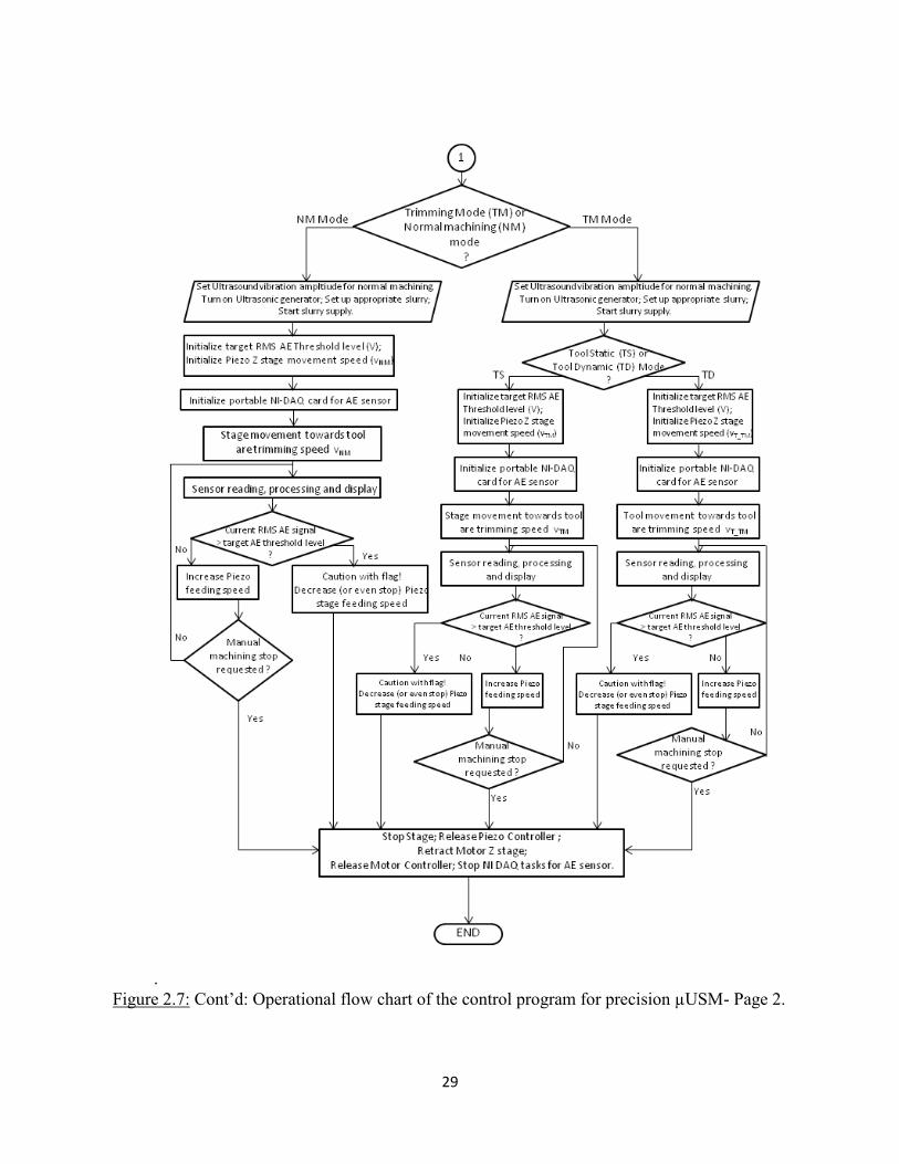
29

.

Figure 2.7: Cont’d: Operational flow chart of the control program for precision µUSM- Page 2.

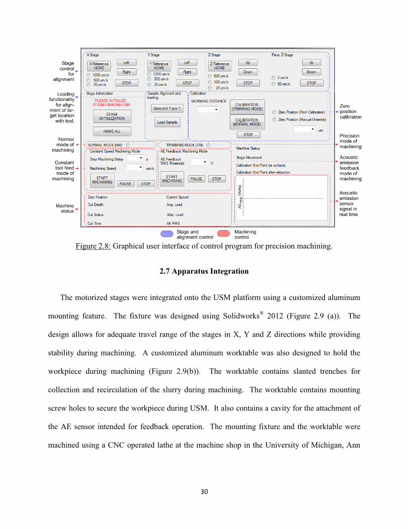
30

Figure 2.8: Graphical user interface of control program for precision machining.

2.7 Apparatus Integration

The motorized stages were integrated onto the USM platform using a customized aluminum

mounting feature. The fixture was designed using Solidworks® 2012 (Figure 2.9 (a)). The

design allows for adequate travel range of the stages in X, Y and Z directions while providing

stability during machining. A customized aluminum worktable was also designed to hold the

workpiece during machining (Figure 2.9(b)). The worktable contains slanted trenches for

collection and recirculation of the slurry during machining. The worktable contains mounting

screw holes to secure the workpiece during USM. It also contains a cavity for the attachment of

the AE sensor intended for feedback operation. The mounting fixture and the worktable were

machined using a CNC operated lathe at the machine shop in the University of Michigan, Ann

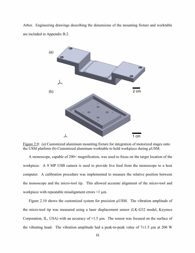
31

Arbor. Engineering drawings describing the dimensions of the mounting fixture and worktable

are included in Appendix B.2.

Figure 2.9: (a) Customized aluminum mounting fixture for integration of motorized stages onto

the USM platform (b) Customized aluminum worktable to hold workpiece during µUSM.

A monoscope, capable of 200× magnification, was used to focus on the target location of the

workpiece. A 9 MP USB camera is used to provide live feed from the monoscope to a host

computer. A calibration procedure was implemented to measure the relative position between

the monoscope and the micro-tool tip. This allowed accurate alignment of the micro-tool and

workpiece with repeatable misalignment errors <1 µm.

Figure 2.10 shows the customized system for precision µUSM. The vibration amplitude of

the micro-tool tip was measured using a laser displacement sensor (LK-G32 model, Keyence

Corporation, IL, USA) with an accuracy of ≈1.5 µm. The sensor was focused on the surface of

the vibrating head. The vibration amplitude had a peak-to-peak value of 7±1.5 µm at 200 W

32

input power. The lateral vibration of a 2-mm long tool was <1.5 µm. Table 2.1 compares

important parameters of a conventional µUSM system and the customized system for precision

µUSM. The smaller vibration amplitudes and high resolution automated stages provide a

platform upon which precision in µUSM can be further explored.

Figure 2.10: Photograph of the customized µUSM system showing various components.

Table 2.1: Comparison of conventional µUSM system parameters with that of the customized

system for precision µUSM. Conventional

µUSM system High precision

µUSM system

Power supply 200-1000 W 200-1000 W

Coupler 1:1 1:2

Measured peak-peak vibration (µm)

15 µm @ P=20%

7 ± 1.5 @ P=20%

Vibration freq. (kHz) 20 20

Z-axis resolution >1 µm 50 nm

33

CHAPTER 3

Micro Ultrasonic Machining based High Resolution Trimming of Ceramics

Introduction

Refinement of µUSM that leads to high resolution µUSM (HR-µUSM) is of potential interest

for the trimming of 3-D microstructures. The two most important attributes of HR-µUSM are

low machining rates, and smooth surfaces. Low machining rates can provide improved control

of machining in the vertical (depth) direction. While the lateral feature sizes depend on the

cutting tools, the material removal rate is determined mainly by the impact velocity of the

abrasive particles. This velocity is a function of the frequency and the amplitude of the vibrating

tool as well as the separation between the tool and the workpiece [Kom93]. In contrast, the

surface finish depends on the particle size of the abrasive used in the ultrasonic machining. For

HR-µUSM trimming with high resolution and high surface quality, several

challenges/requirements need to be addressed. These included: 1) tool miniaturization; 2) fixed

tool position for reduced machining rates; 3) effect of low vibration amplitude; 4) effect of small

abrasive particles; 5) minimization of unwanted acoustic coupling to avoid damaging fragile, 3-

D workpiece structures.

Need for post fabrication trimming using HR-µUSM

Post fabrication trimming using HR-µUSM can be potentially used for a number of MEMS

applications which require high resolution mass removal from 3-D microstructures, while

providing good surface finishes. In particular, it is appealing for the post-fabrication trimming of

34

inertial sensors, timing references and mass-balance resonators to adjust stiffness, mass and

potentially damping [Kem11], [Pue12]. Non-planar geometries and technologies in resonant

MEMS have been investigated in the recent past to provide improved symmetry, reduced surface

roughness and increased aspect ratios. These investigations have led to the development of

hemispherical glass blown structures for use as resonators and gyroscopes [Cho14], [Shk11].

The trimming of these devices is necessary for improving its structural symmetry and thus their

performance. The trimming of these 3-D microstructures is a challenge for traditional

lithographic processes, due to the difficulties associated with spinning and patterning photoresist

on such structures. Laser trimming is also a challenge because of the transparency of the

material.

Section 3.1 describes the concept of the HR-μUSM operation. Section 3.2 describes the

analytical and numerical modeling of the HR-μUSM process. Section 3.3 describes the

experimental evaluation of the HR-μUSM process. In particular, a quantitative evaluation of the

impact of particle size, slurry behavior, micro-tool position, and micro-tool amplitude on

machining rates and surface roughness is performed. Section 3.4 evaluates HR-µUSM for the

trimming of hemispherical 3-D microstructures. In this context, trimming is defined as the

procedure by which small quantities of mass can be removed from selected locations. Section

3.5 presents a discussion and the conclusions.

3.1 Process Description

The HR-µUSM concept is illustrated in Figure 3.1. The micro-tool tip is positioned at a

predefined fixed distance (FD) from the workpiece, without micro-tool feed toward the

workpiece as in conventional µUSM. Low vibration amplitudes and small abrasive particles are

used to further reduce the machining rates and provide superior surface finish.

35

Figure 3.1: Conceptual comparison of micro ultrasonic machining (µUSM) used for

conventional µUSM and for HR-µUSM. (a) Conventional µUSM produces deeper machined

features with rougher surfaces. (b) HR-µUSM uses greater, fixed, distances between tool and

workpiece, smaller abrasive particles and lower tool vibration amplitude.

3.2 Analytical and Numerical Study

Analytical Study

Various analytical models exist in literature to predict the machining rates of stationary

µUSM as a function of process parameters. A majority of these are first order models based on

statistical analysis and provide an estimation of USM behavior. Shaw’s model provides an

equation for material removal rate due to hammering action of the abrasive particles on the

workpiece [Sha56b]. Miller proposed another equation for the material removal rate taking into

consideration the amount of plastic deformation undergone by the workpiece per blow and other

parameters [Mil57]. Cook estimated the penetration rate as a function of common USM

parameters such as the vibration amplitude, frequency, abrasive particle sizes and the workpiece

hardness [Coo66]. Since these were the parameters of interest for HR-µUSM, Cook’s model

was used in this analytical study. In this model the machining rate (MR) in the vertical direction

(in mm·s-1

), or the penetration rate, can be expressed by [Coo66]:

(1)

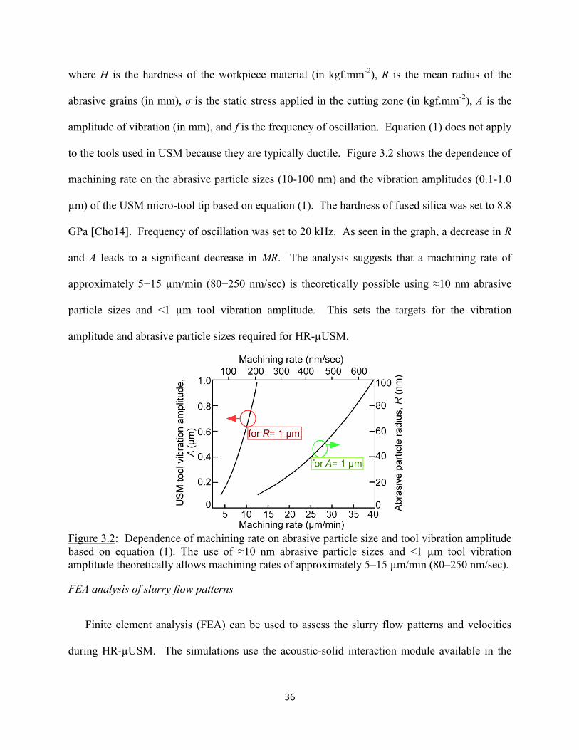
36

where H is the hardness of the workpiece material (in kgf.mm-2

), R is the mean radius of the

abrasive grains (in mm), σ is the static stress applied in the cutting zone (in kgf.mm-2

), A is the

amplitude of vibration (in mm), and f is the frequency of oscillation. Equation (1) does not apply

to the tools used in USM because they are typically ductile. Figure 3.2 shows the dependence of

machining rate on the abrasive particle sizes (10-100 nm) and the vibration amplitudes (0.1-1.0

µm) of the USM micro-tool tip based on equation (1). The hardness of fused silica was set to 8.8

GPa [Cho14]. Frequency of oscillation was set to 20 kHz. As seen in the graph, a decrease in R

and A leads to a significant decrease in MR. The analysis suggests that a machining rate of

approximately 5−15 µm/min (80−250 nm/sec) is theoretically possible using ≈10 nm abrasive

particle sizes and <1 µm tool vibration amplitude. This sets the targets for the vibration

amplitude and abrasive particle sizes required for HR-µUSM.

Figure 3.2: Dependence of machining rate on abrasive particle size and tool vibration amplitude

based on equation (1). The use of ≈10 nm abrasive particle sizes and <1 µm tool vibration

amplitude theoretically allows machining rates of approximately 5–15 µm/min (80–250 nm/sec).

FEA analysis of slurry flow patterns

Finite element analysis (FEA) can be used to assess the slurry flow patterns and velocities

during HR-µUSM. The simulations use the acoustic-solid interaction module available in the

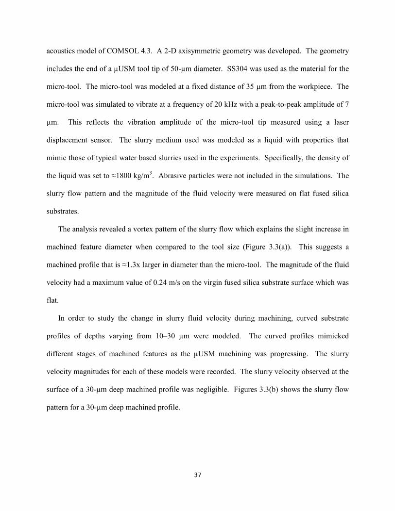
37

acoustics model of COMSOL 4.3. A 2-D axisymmetric geometry was developed. The geometry

includes the end of a µUSM tool tip of 50-µm diameter. SS304 was used as the material for the

micro-tool. The micro-tool was modeled at a fixed distance of 35 µm from the workpiece. The

micro-tool was simulated to vibrate at a frequency of 20 kHz with a peak-to-peak amplitude of 7

µm. This reflects the vibration amplitude of the micro-tool tip measured using a laser

displacement sensor. The slurry medium used was modeled as a liquid with properties that

mimic those of typical water based slurries used in the experiments. Specifically, the density of

the liquid was set to ≈1800 kg/m3. Abrasive particles were not included in the simulations. The

slurry flow pattern and the magnitude of the fluid velocity were measured on flat fused silica

substrates.

The analysis revealed a vortex pattern of the slurry flow which explains the slight increase in

machined feature diameter when compared to the tool size (Figure 3.3(a)). This suggests a

machined profile that is ≈1.3x larger in diameter than the micro-tool. The magnitude of the fluid

velocity had a maximum value of 0.24 m/s on the virgin fused silica substrate surface which was

flat.

In order to study the change in slurry fluid velocity during machining, curved substrate

profiles of depths varying from 10–30 µm were modeled. The curved profiles mimicked

different stages of machined features as the µUSM machining was progressing. The slurry

velocity magnitudes for each of these models were recorded. The slurry velocity observed at the

surface of a 30-µm deep machined profile was negligible. Figures 3.3(b) shows the slurry flow

pattern for a 30-µm deep machined profile.

38

Figure 3.3: Results of FEA analysis showing slurry flow patterns during HR-µUSM of different

workpiece profiles (a) Vortex slurry flow pattern seen on a flat surface. The maximum slurry

velocity observed on a flat fused silica substrate is 0.24 m/s. (b) Slurry flow pattern for a curved

profile of 30-µm depth. Maximum fluid velocity observed on curved surface is negligible.

3.3 Process Characterization on Flat Fused Silica Substrates

Experimental methods

The HR-μUSM process characterization was performed on flat fused silica workpieces of 90-

µm thickness and 4×4 mm2 area. These characterizations aim to evaluate the impact of particle

size, slurry behavior, micro-tool position, and micro-tool amplitude on machining rates and

surface roughness. The precision μUSM system described in Chapter 2 was used as the

machining apparatus. Machining was performed in the serial mode using a 50-µm SS304 micro-

tool fabricated using the procedure outlines in Chapter 2, Section 2.5. The slurry powders used

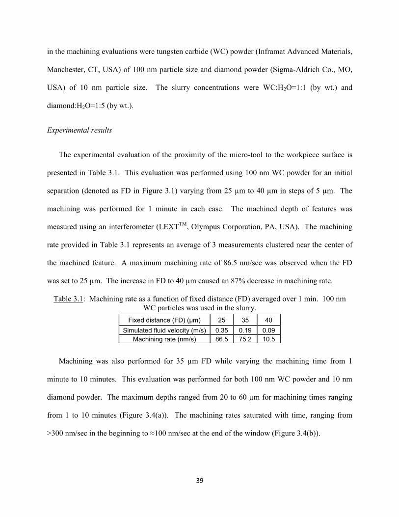
39

in the machining evaluations were tungsten carbide (WC) powder (Inframat Advanced Materials,

Manchester, CT, USA) of 100 nm particle size and diamond powder (Sigma-Aldrich Co., MO,

USA) of 10 nm particle size. The slurry concentrations were WC:H2O=1:1 (by wt.) and

diamond:H2O=1:5 (by wt.).

Experimental results

The experimental evaluation of the proximity of the micro-tool to the workpiece surface is

presented in Table 3.1. This evaluation was performed using 100 nm WC powder for an initial

separation (denoted as FD in Figure 3.1) varying from 25 µm to 40 µm in steps of 5 µm. The

machining was performed for 1 minute in each case. The machined depth of features was

measured using an interferometer (LEXTTM

, Olympus Corporation, PA, USA). The machining

rate provided in Table 3.1 represents an average of 3 measurements clustered near the center of

the machined feature. A maximum machining rate of 86.5 nm/sec was observed when the FD

was set to 25 µm. The increase in FD to 40 µm caused an 87% decrease in machining rate.

Table 3.1: Machining rate as a function of fixed distance (FD) averaged over 1 min. 100 nm

WC particles was used in the slurry.

Machining was also performed for 35 µm FD while varying the machining time from 1

minute to 10 minutes. This evaluation was performed for both 100 nm WC powder and 10 nm

diamond powder. The maximum depths ranged from 20 to 60 µm for machining times ranging

from 1 to 10 minutes (Figure 3.4(a)). The machining rates saturated with time, ranging from

>300 nm/sec in the beginning to ≈100 nm/sec at the end of the window (Figure 3.4(b)).

Fixed distance (FD) (µm) 25 35 40

Simulated fluid velocity (m/s) 0.35 0.19 0.09

Machining rate (nm/s) 86.5 75.2 10.5

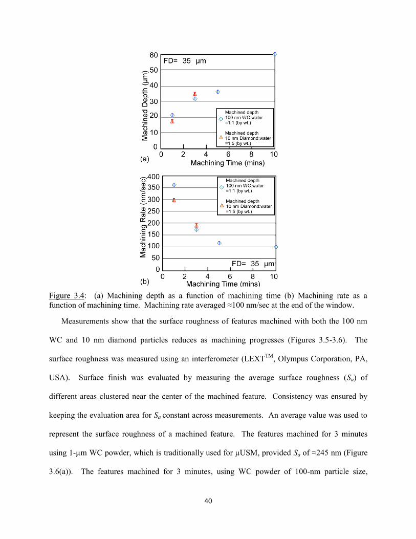
40

Figure 3.4: (a) Machining depth as a function of machining time (b) Machining rate as a

function of machining time. Machining rate averaged ≈100 nm/sec at the end of the window.

Measurements show that the surface roughness of features machined with both the 100 nm

WC and 10 nm diamond particles reduces as machining progresses (Figures 3.5-3.6). The

surface roughness was measured using an interferometer (LEXTTM

, Olympus Corporation, PA,

USA). Surface finish was evaluated by measuring the average surface roughness (Sa) of

different areas clustered near the center of the machined feature. Consistency was ensured by

keeping the evaluation area for Sa constant across measurements. An average value was used to

represent the surface roughness of a machined feature. The features machined for 3 minutes

using 1-µm WC powder, which is traditionally used for µUSM, provided Sa of ≈245 nm (Figure

3.6(a)). The features machined for 3 minutes, using WC powder of 100-nm particle size,

41

provided Sa of ≈85 nm (Figures 3.5 and 3.6(b)). The Sa for features machined with 10 nm

diamond slurry powder was ≈30 nm (Figures 3.5 and 3.6(c,d)). The Sa of the virgin fused silica

substrate was ≈5 nm. The average surface roughness achievable using conventional µUSM

utilized in past work is typically 200-400 nm [Mas96], [Li06], [Li14], [Raj06]. Table 3.2

provides the typical surface roughness parameters evaluated at six different areas in a feature

machined using 10 nm diamond slurry powder (Figure 3.6(c)). The Sa of features machined with

10 nm diamond particles is ≈7× smaller than typical conventional µUSM.

Figure 3.5: Average surface roughness, Sa, as a function of machining time. The minimum Sa

observed was 30 nm; this was obtained with 10 nm diamond powder in 3 minutes.

Another parameter that can be used to assess surface quality is Sp, which represents the

maximum height of peaks. In this work, for samples machined with 10 nm diamond particles,

the Sp was ≈250 nm. The Sp can be greater than Sa due to factors such as minor imperfections of

the tool and residual particles on the workpiece. A single defect can increase Sp even though the

average roughness, as represented by Sa, may not be significantly affected by it. The average

parameter Sa provides a surface roughness that better represents the majority of the area that has

been machined and has been typically used to assess surface quality of machined features

[Mas96],[Li06], [Li14], [Raj06].

42

Figure 3.6: SEM images of machined features using: (a) Tungsten Carbide (1 µm, WC:H2O=1:1

by wt.). The machined feature diameter was 73 µm. The corresponding average surface

roughness, Sa, was 245 nm. (b) Tungsten Carbide (100 nm). The machined feature diameter was

69 µm. The corresponding Sa was 67 nm. (c) Diamond (10 nm) slurry. The machined feature

diameter was 75 µm. The corresponding Sa was 30 nm. Each machining was performed for 2

minutes. (d) A typical profile of the machined feature using diamond (10 nm) slurry. Measured

values of Sa at locations 1-6 denoted in (c) are provided in Table 3.2.

43

Table 3.2: Average surface roughness (Sa) measured at six different areas of a feature machined

with 10 nm diamond slurry powder (Figure 3.6(c)). Evaluation area Sa (nm)

1 31

2 37

3 31

4 29

5 33

6 27

Average ≈30

The average volume removed from virgin flat fused silica substrates in the first minute was

≈9.1×10-6

mm3. This corresponds to a mass removal of ≈20 ng/min. This estimate assumes that

the machined profile can be approximated by a cone frustum. The wear length of the tool after

machining of flat fused silica substrates was ≈1 µm. This corresponds to a tool wear ratio (i.e.

ratio of the tool height worn to the machined depth) of <4 %.

Table 3.3 summarizes the machining results. At 40-µm FD, the HR-µUSM process achieved

cutting rates as low as 10 nm/sec. The average surface roughness, Sa, achieved was ≈30 nm

using 10 nm diamond particles in the slurry medium.

Table 3.3: Machining results for HR-µUSM

Abrasive: avg. size (nm) WC:100 Diamond:10

Min. cutting rate (nm/sec)

10 ≈10

Roughness (Sa) (nm) >60 30 or better

3.4 Trimming of 3-D Fused Silica Microshells

The HR-µUSM process was applied to the trimming of hemispherical 3-D microstructures

made of fused silica. For this work, bird-bath (BB) shells (Figure 3.7(a)), which are being

investigated for use in rate integrating gyroscopes [Cho14], were used. These structures have a

diameter of 5 mm, and height of 1.55 mm, whereas the average thickness of the shell is only 70

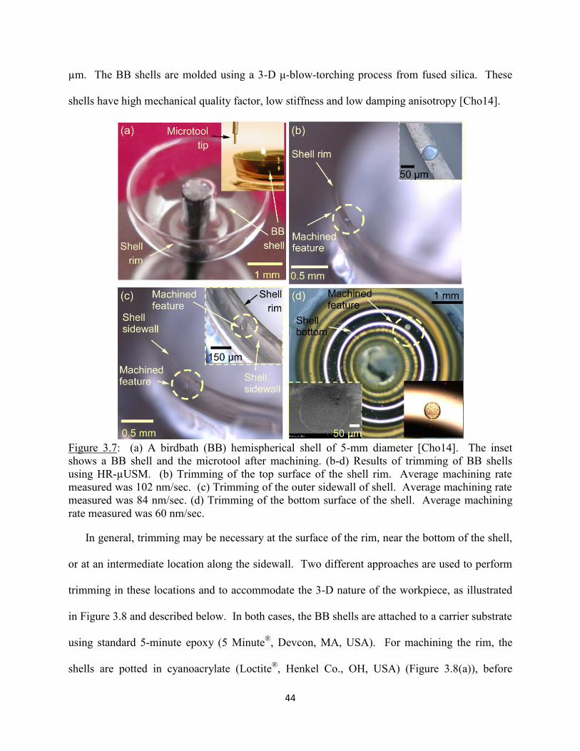
44

µm. The BB shells are molded using a 3-D μ-blow-torching process from fused silica. These

shells have high mechanical quality factor, low stiffness and low damping anisotropy [Cho14].

Figure 3.7: (a) A birdbath (BB) hemispherical shell of 5-mm diameter [Cho14]. The inset

shows a BB shell and the microtool after machining. (b-d) Results of trimming of BB shells

using HR-µUSM. (b) Trimming of the top surface of the shell rim. Average machining rate

measured was 102 nm/sec. (c) Trimming of the outer sidewall of shell. Average machining rate

measured was 84 nm/sec. (d) Trimming of the bottom surface of the shell. Average machining

rate measured was 60 nm/sec.

In general, trimming may be necessary at the surface of the rim, near the bottom of the shell,

or at an intermediate location along the sidewall. Two different approaches are used to perform

trimming in these locations and to accommodate the 3-D nature of the workpiece, as illustrated

in Figure 3.8 and described below. In both cases, the BB shells are attached to a carrier substrate

using standard 5-minute epoxy (5 Minute®, Devcon, MA, USA). For machining the rim, the

shells are potted in cyanoacrylate (Loctite®, Henkel Co., OH, USA) (Figure 3.8(a)), before

45

immersing in slurry. This arrangement provides mechanical support for the 70-µm-thick shell

walls, and also reduces the topographical variation, allowing the slurry flow to be similar to that

for a flat substrate. This arrangement is also used when machining the sidewalls. For machining

the bottom, the potting is not needed. Instead, slurry is filled into the shell, and a long tool (5–10

mm in length) is used to perform the trimming (Figure 3.8(b)). The slurry meniscus does not

contact the tool holder, so the ultrasonic power is not directly transferred into the slurry. This

reduces the propensity for damage to the fragile shell. The machined depth and surface

roughness of features in the BB shells were measured using an interferometer (LEXTTM

,

Olympus Corporation, PA, USA). The BB shells were coated with a ≈5 nm gold layer prior to

measurement. This was done in order to facilitate laser interferometry and SEM imaging of the

transparent and nonconductive fused silica shells, without significantly affecting the depth and

roughness measurements.

Figure 3.7(b) shows a typical machined feature on the rim of the shell. Machining with 100

nm WC for 180 seconds provided an average depth of 18 µm, diameter of 60 µm, and roughness

Sa of 120-150 nm. The tool diameter was 60 µm, and it was 2 mm long. Figure 3.7(c) shows a

typical sidewall machined cavity. A machining time of 300 seconds provided a cavity with a

typical maximum depth of 25 µm using 100 nm WC. The tool diameter and length were 120 µm

and 5 mm, respectively. Figure 3.7(d) shows a typical machined cavity on the bottom surface of

the shell. Tools of 120-µm diameter and 5 mm length were used. A machining time of 150

seconds, with 100 nm WC, provided features with 9-µm depth and 140-µm diameter. Compared

to machining of the rim, the decrease in machining rate can be attributed to the smaller number

of abrasive particles available for circulation in the cutting zone: some particles settle at the

bottom of the shell and do not contribute to the machining. The average machining rate obtained

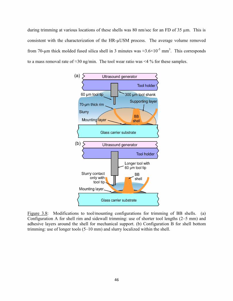
46

during trimming at various locations of these shells was 80 nm/sec for an FD of 35 µm. This is

consistent with the characterization of the HR-µUSM process. The average volume removed

from 70-µm thick molded fused silica shell in 3 minutes was ≈3.6×10-5

mm3. This corresponds

to a mass removal rate of ≈30 ng/min. The tool wear ratio was <4 % for these samples.

Figure 3.8: Modifications to tool/mounting configurations for trimming of BB shells. (a)

Configuration A for shell rim and sidewall trimming: use of shorter tool lengths (2–5 mm) and

adhesive layers around the shell for mechanical support. (b) Configuration B for shell bottom

trimming: use of longer tools (5–10 mm) and slurry localized within the shell.

47

3.5 Discussion and Conclusions

The micro-tool fabrication sequence allows for flexibility of choice of micro-tool diameter

and lengths. However, there are certain limitations to this technique. This is a serial process and

involves manual mounting of a single micro-tool onto the USM tool head. This can be resolved

by fabricating an array of micro-tools using the batch pattern transfer technique. Another

limitation is the micro-tool mounting error, i.e., the error in the orthogonality between the micro-

tool and the workpiece. Although this does not have a major impact when machined features are

shallow, such as those used for trimming, the tolerance is lower for deeper features. A

monolithic approach to micro-tool fabrication will diminish this.

The typical machining rates of HR-µUSM demonstrated in this work averaged ≈100 nm/sec,

for 35 µm FD. The minimum machining rate was 10 nm/sec, for 40 µm FD. This is an

improvement in machining resolution over conventional machining technologies. The average

mass of fused silica removed from a flat virgin sample in the first minute was ≈20 ng. An

average surface roughness (Sa) of 30 nm was achieved by machining with 10 nm diamond

abrasive particles in the slurry. This is ≈7× smaller than typical conventional µUSM. The virgin

fused silica workpiece surface has an average Sa of ≈5 nm and provides a quantitative

comparison of smoothness achieved by HR-µUSM. It can be inferred by the experimental

analysis that while the machining rate is influenced more by the separation between the tool and

the workpiece, the surface roughness depends mainly on the abrasive particle size. A further

decrease in vibration amplitude and abrasive particle sizes will facilitate lower machining rates

and smoother profiles than that achieved in this work. The process was demonstrated for

trimming of hemispherical 3-D shells made of fused silica. Cavities were successfully formed

on the thin shell rim with controlled depths and machining rates.

48

A disadvantage of the HR-µUSM process was the quick precipitation of the slurry which

significantly lowered the machining rates. This necessitated additional mounting configurations

for the µUSM 3-D workpieces. These additional steps increase the complexity associated with

the machining of 3-D structures and therefore restricts its throughput. A process can be

envisioned in which the workpiece is vibrated and not the tool. This would keep the abrasive

particles in the slurry agitated during µUSM operation. Batch-mode µUSM using workpiece

vibration in µUSM is explored in Chapter 4.

49

CHAPTER 4

Batch-mode µUSM using Workpiece Vibration

This chapter describes μUSM process variations in pursuit of two goals. The first is to

eliminate slurry precipitation or settling that presents a challenge for 3-D machining. The second

is to investigate the viability of silicon microstructures as μUSM tools. This would allow the

possibility of using fine-featured cutting tools that can be fabricated by deep reactive ion etching

(DRIE).

Section 4.1 describes the concept of batch-mode μUSM operation using workpiece vibration

to eliminate slurry precipitation. Section 4.2 details machining results obtained using workpiece

vibration, in particular, the influence of μUSM parameters on machining rates and surface

roughness. Section 4.3 describes the batch-mode machining using a micro-tool array of 50-μm

feature sizes fabricated by μEDM. Section 4.4 describes the evaluation of DRIE silicon micro-

tools for batch mode ultrasonic machining of (sub-10 µm features in) fused silica. Section 4.5

presents a discussion and the conclusions.

4.1 Workpiece Vibration

Approach

Traditionally, in the μUSM process, the vibration of the tool imparts momentum to the

abrasive particles suspended in the slurry which bombards the workpiece, causing machining.

The high resolution μUSM process described in Chapter 3 follows this approach for machining.

A complementary approach can be envisioned in which the workpiece is vibrated while the tool

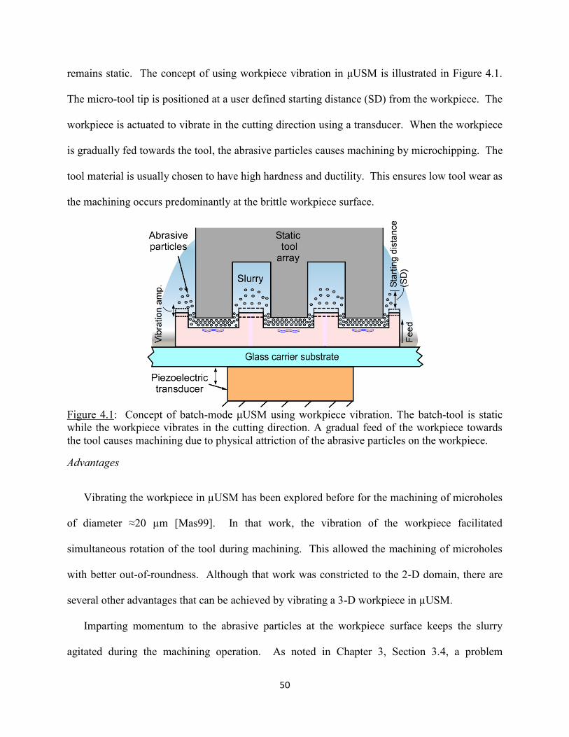
50

remains static. The concept of using workpiece vibration in μUSM is illustrated in Figure 4.1.

The micro-tool tip is positioned at a user defined starting distance (SD) from the workpiece. The

workpiece is actuated to vibrate in the cutting direction using a transducer. When the workpiece

is gradually fed towards the tool, the abrasive particles causes machining by microchipping. The

tool material is usually chosen to have high hardness and ductility. This ensures low tool wear as

the machining occurs predominantly at the brittle workpiece surface.

Figure 4.1: Concept of batch-mode μUSM using workpiece vibration. The batch-tool is static

while the workpiece vibrates in the cutting direction. A gradual feed of the workpiece towards

the tool causes machining due to physical attriction of the abrasive particles on the workpiece.

Advantages

Vibrating the workpiece in µUSM has been explored before for the machining of microholes

of diameter ≈20 µm [Mas99]. In that work, the vibration of the workpiece facilitated

simultaneous rotation of the tool during machining. This allowed the machining of microholes

with better out-of-roundness. Although that work was constricted to the 2-D domain, there are

several other advantages that can be achieved by vibrating a 3-D workpiece in µUSM.

Imparting momentum to the abrasive particles at the workpiece surface keeps the slurry

agitated during the machining operation. As noted in Chapter 3, Section 3.4, a problem

51

encountered during machining of fragile 3-D structures is the settling out of the slurry, which

drastically reduces the machining rates to negligible values. This necessitated additional

mounting configurations to accommodate the 3-D nature of the workpiece. These additional

steps increase the complexity associated with the machining of 3-D structures and therefore

restricts its throughput. In this regard, the vibration of the workpiece helps reduce slurry settling,

enabling the μUSM of 3-D workpieces.

Mechanism of machining

The mechanism of machining using workpiece vibration is illustrated in Figure 4.1. As the

workpiece is fed towards the tool, the tool-workpiece gap decreases gradually. The vibration of

the workpiece agitates the abrasive particles. Machining occurs due to physical attrition of the

workpiece by the trapped abrasive particles and may be enhanced by debris trapped in the

narrow gap between the tool and the workpiece. The slurry supplies fresh abrasive materials to

the cutting zone and removes debris from the cutting area. The slurry also acts as a coolant to

prevent any potential temperature rise as a result of the attrition process.

Choice of transducer to vibrate the workpiece

Piezoelectric lead zirconate titanate (PZT) transducers have been used widely to convert

electrical signals into mechanical vibrations. They have several advantages over electrostatic

and electromagnetic transduction mechanisms. They offer superior linearity over a wide input

amplitude range. The vibration amplitudes achievable using PZT stacks can range from 1–50

μm, which is ideal for the μUSM operation. In fact, most ultrasonic generators contain

piezoelectric discs to generate vibrations (with amplitudes ranging from 0.001–0.1 μm) that are

subsequently amplified using a horn to generate larger tool vibration [Tho98]. Stacking a

52

number of these piezoelectric discs provides a large (1–50 μm) vibration amplitude without the

need for a mechanical horn to perform amplification.

Piezo stack actuators are available commercially and cater to high force, large displacement,

and high mass loading applications. A high force, stack actuator (P.885.51 PICMA® from

Physik Instrumente, Inc.) was used to vibrate the workpiece. A photograph of the actuator is

shown in Figure 4.2. The relevant specifications of this device are provided in Table 4.1.

Figure 4.2: P.885.51 PICMA

® multilayer stack actuator [Phy14].

Table 4.1: Relevant device specifications of the P.885.51 PICMA® multilayer stack actuator

Maximum displacement (µm) 18±10%

Recommended preload for dynamic operation (MPa)

15

Resonant frequency (kHz) 70

Operating voltage (V) -20 to +120

Stiffness (N/µm) 50

Tool preparation for batch mode μUSM

As described in Chapter 1, Section 1.3, a batch mode operation in μUSM greatly enhances

the throughput of the process and provides the ability to transfer complex patterns onto ceramic

substrates. The fabrication of batch tools in µUSM can be non-lithographically based (NLB) as

well as lithographically based (LB). Processes such as μEDM can be used to fabricate micro-

53

tool arrays for USM with feature sizes ≥5 µm [Raj06], [Li06], [Li13]. Serial micro EDM can be

used to transfer simple tool patterns with relative ease onto stainless steel substrates [Li06]. This

process is suitable for rapid prototyping of machining processes. In order to truly improve the

throughput and the ability to machine complex patterns, it is desired to fabricate micro-tools

lithographically. As mentioned in chapter 1, Section 1.3, a process (named LEEDUS: a

combination of lithography, electroplating, μEDM and μUSM) allowing batch-mode pattern

transfer onto ceramic dies was described in [Li06]. In this process, an electroplating mold is first

created on a silicon or metal wafer using standard lithography, then using the electroplated

pattern as an electrode to EDM a hard metal (stainless steel or WC/Co) tool, which is finally

used in the USM of the ceramic substrate. The machining rates achieved in that work were ≥18

μm/min. The corresponding surface finish, Ra, of machined features ranged from 0.4–0.7 μm.

In this work, micro-tools for batch-mode μUSM are fabricated using two processes. Firstly,

a micro-tool array of 50-μm feature sizes is fabricated by serial μEDM. Secondly, the

fabrication of micro-tools using DRIE of silicon is explored. The DRIE process allows the

fabrication of fine features Si micromachined tools intended for the batch mode ultrasonic

machining of (sub-10 µm features in) fused silica. This greatly enhances the throughput of the

μUSM process.

4.2 Process Characterization

4.2.1 Workpiece vibration amplitude

To characterize the vibration amplitude of the piezoelectric transducer used for workpiece

vibration, a setup illustrated in Figure 4.3 was used. The transducer was loaded with a glass

54

carrier slide, workpiece and slurry to mimic the weight that the transducer was subjected to

during the μUSM operation

Figure 4.3: Schematic of setup used to measure vibration amplitude of the workpiece.

A laser displacement sensor (LK-G32 model, Keyence Corporation, IL, USA) having an

accuracy of ±0.5 μm was used to measure the vibration amplitude of the workpiece surface. For

efficient measurement, it is important to ensure that the sampling frequency be set to atleast 10×

the PZT stack actuation frequency. Fortunately, the PZT stack provides constant vibration

amplitudes over a wide range of frequencies (10 Hz to 40 kHz) for a particular actuation voltage.

A typical vibration amplitude plot of a loaded PZT stack is shown in Figure 4.4. A load ≈25 g

comprises of a glass carrier slide, a workpiece, clay slurry reservoirs and slurry and reflects the

static load on the PZT during μUSM. The workpiece vibration amplitude shows a fairly linear

increase with an increase in PZT transducer actuation voltage. The amplitude ranges from 1–10

μm for varying actuation voltage levels. These amplitude levels lie in the range of typical

ultrasonic vibrations used in μUSM.

55

Figure 4.4: Vibration amplitude of the workpiece as a function of PZT actuation voltage. The

PZT was loaded with 25 g weight comprising of glass slide, workpiece, clay reservoir and slurry.

4.2.2 Machining rate and surface roughness dependence on μUSM parameters

The machining rate (MR) and surface roughness (Sa) dependence on the workpiece vibration

amplitude was characterized. The characterization was done in the serial mode using a stainless

steel micro-tool having 50-µm tip diameter. This vibration amplitude can be controlled by

varying the input actuation voltage to the piezoelectric transducer as seen in Figure 4.4. The

characterizations were performed on fused silica (FS) substrates. The process control software

described in Chapter 2, Section 2.6 is used to perform the stage movement control and tool

touch-off detection functionalities. There was no machining feed between the tool and the

workpiece in order to ensure that the relative proximity of the tool to workpiece is only

dependent on the workpiece vibration amplitude. The machining parameters used for these

characterizations are summarized in Table 4.2.

Table 4.2: Machining parameters used for characterization of machining rate, MR, and surface

roughness, Sa, on workpiece vibration amplitude. Workpiece Fused silica, flat, 4×4

mm2, 90 µm thickness

Transducer actuation voltage 10–70 Vp-p

Vibration amplitude range (µm) 0.7–8.3

PZT actuation frequency 20 kHz

Fixed distance (FD) 12 µm

Machining time 5 mins.

Slurry type WC(100 nm):H20::1:1 (by wt.)

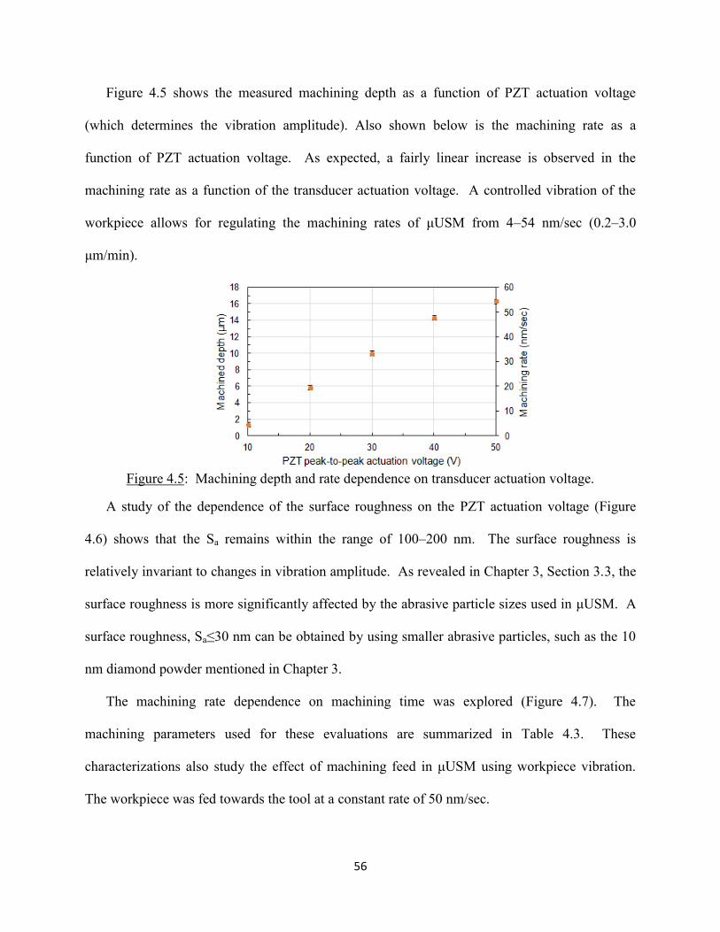
56

Figure 4.5 shows the measured machining depth as a function of PZT actuation voltage

(which determines the vibration amplitude). Also shown below is the machining rate as a

function of PZT actuation voltage. As expected, a fairly linear increase is observed in the

machining rate as a function of the transducer actuation voltage. A controlled vibration of the

workpiece allows for regulating the machining rates of μUSM from 4–54 nm/sec (0.2–3.0

μm/min).

Figure 4.5: Machining depth and rate dependence on transducer actuation voltage.

A study of the dependence of the surface roughness on the PZT actuation voltage (Figure

4.6) shows that the Sa remains within the range of 100–200 nm. The surface roughness is

relatively invariant to changes in vibration amplitude. As revealed in Chapter 3, Section 3.3, the

surface roughness is more significantly affected by the abrasive particle sizes used in μUSM. A

surface roughness, Sa≤30 nm can be obtained by using smaller abrasive particles, such as the 10

nm diamond powder mentioned in Chapter 3.

The machining rate dependence on machining time was explored (Figure 4.7). The

machining parameters used for these evaluations are summarized in Table 4.3. These

characterizations also study the effect of machining feed in μUSM using workpiece vibration.

The workpiece was fed towards the tool at a constant rate of 50 nm/sec.

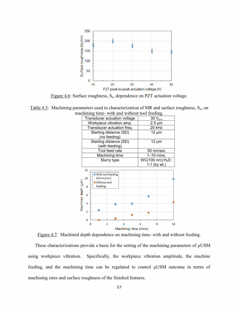
57

Figure 4.6: Surface roughness, Sa, dependence on PZT actuation voltage.

Table 4.3: Machining parameters used in characterization of MR and surface roughness, Sa, on

machining time- with and without tool feeding. Transducer actuation voltage 30 Vp-p

Workpiece vibration amp. 2.5 µm

Transducer actuation freq. 20 kHz

Starting distance (SD) (no feeding)

12 µm

Starting distance (SD) (with feeding)

12 µm

Tool feed rate 50 nm/sec

Machining time 1–10 mins.

Slurry type WC(100 nm):H20:: 1:1 (by wt.)

Figure 4.7: Machined depth dependence on machining time- with and without feeding.

These characterizations provide a basis for the setting of the machining parameters of μUSM

using workpiece vibration. Specifically, the workpiece vibration amplitude, the machine

feeding, and the machining time can be regulated to control μUSM outcome in terms of

machining rates and surface roughness of the finished features.

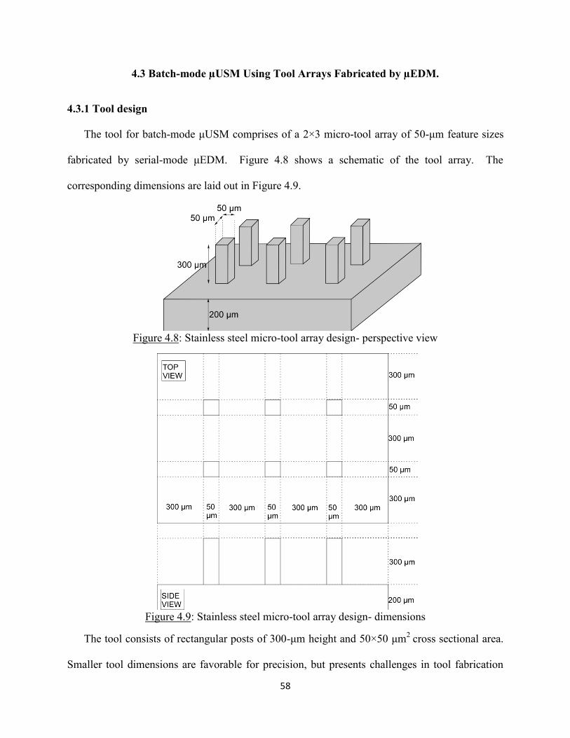
58

4.3 Batch-mode µUSM Using Tool Arrays Fabricated by µEDM.

4.3.1 Tool design

The tool for batch-mode μUSM comprises of a 2×3 micro-tool array of 50-μm feature sizes

fabricated by serial-mode μEDM. Figure 4.8 shows a schematic of the tool array. The

corresponding dimensions are laid out in Figure 4.9.

Figure 4.8: Stainless steel micro-tool array design- perspective view

Figure 4.9: Stainless steel micro-tool array design- dimensions

The tool consists of rectangular posts of 300-μm height and 50×50 μm2

cross sectional area.

Smaller tool dimensions are favorable for precision, but presents challenges in tool fabrication

59

and handling. The 2×3 array size requires less time for machining and is intended for rapid

proof-of-concept of batch fabrication. The micro-tool array can be extended to larger sizes at the

cost of more machining time.

The material used for the micro-tool should have high wear resistance, favorable elastic and

fatigue strength properties, toughness, and hardness [McG88], [Ken75], [Nep56]. Stainless steel

tools have a lower tool wear ratio, i.e. the ratio of the tool height worn to the machined depth

[Li06]. As the tool is not actuated using the ultrasound generator in this process, there are no

stringent requirements for the weight of the tool to be within the loading limits of an ultrasound

horn. This provides flexibility for the choice of tool material and dimensions of the tool

substrate which carry the micro patterns to be transferred to the workpiece.

4.3.2 FEA simulation of slurry flow patterns

To help better understand the effect of slurry fluidics on the machining, finite element

analysis (FEA) was used to assess the slurry flow patterns and velocities during batch-mode

µUSM using workpiece vibration. The simulations use the acoustic-solid interaction module

available in the acoustics model of COMSOL 4.3. A 3-D geometry was developed. The

geometry includes a 2×3 array of micro-tools with 50-µm diameter and 300-µm height. SS304

was used as the material for the micro-tool array. The micro-tool was modeled at a fixed

distance of 12 µm from the workpiece. The workpiece was simulated to vibrate at a frequency

of 20 kHz and with a peak-to-peak amplitude of 2.5 µm. This reflects the vibration amplitude of

the workpiece for an actuation voltage of 30 Vp-p applied to the piezoelectric transducer. The

slurry medium used was modeled as a liquid with properties that mimic those of typical water

based slurries used in the experiments. Specifically, the density of the liquid was set to ≈1800

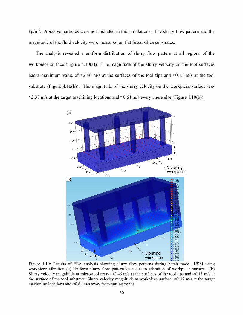
60

kg/m3. Abrasive particles were not included in the simulations. The slurry flow pattern and the

magnitude of the fluid velocity were measured on flat fused silica substrates.

The analysis revealed a uniform distribution of slurry flow pattern at all regions of the

workpiece surface (Figure 4.10(a)). The magnitude of the slurry velocity on the tool surfaces

had a maximum value of ≈2.46 m/s at the surfaces of the tool tips and ≈0.13 m/s at the tool

substrate (Figure 4.10(b)). The magnitude of the slurry velocity on the workpiece surface was

≈2.37 m/s at the target machining locations and ≈0.64 m/s everywhere else (Figure 4.10(b)).

Figure 4.10: Results of FEA analysis showing slurry flow patterns during batch-mode µUSM using

workpiece vibration (a) Uniform slurry flow pattern seen due to vibration of workpiece surface. (b)

Slurry velocity magnitude at micro-tool array: ≈2.46 m/s at the surfaces of the tool tips and ≈0.13 m/s at

the surface of the tool substrate. Slurry velocity magnitude at workpiece surface: ≈2.37 m/s at the target

machining locations and ≈0.64 m/s away from cutting zones.

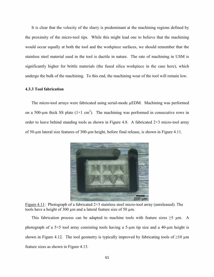
61

It is clear that the velocity of the slurry is predominant at the machining regions defined by

the proximity of the micro-tool tips. While this might lead one to believe that the machining

would occur equally at both the tool and the workpiece surfaces, we should remember that the

stainless steel material used in the tool is ductile in nature. The rate of machining in USM is

significantly higher for brittle materials (the fused silica workpiece in the case here), which

undergo the bulk of the machining. To this end, the machining wear of the tool will remain low.

4.3.3 Tool fabrication

The micro-tool arrays were fabricated using serial-mode µEDM. Machining was performed

on a 500-µm thick SS plate (1×1 cm2). The machining was performed in consecutive rows in

order to leave behind standing tools as shown in Figure 4.8. A fabricated 2×3 micro-tool array

of 50-µm lateral size features of 300-µm height, before final release, is shown in Figure 4.11.

Figure 4.11: Photograph of a fabricated 2×3 stainless steel micro-tool array (unreleased). The

tools have a height of 300 µm and a lateral feature size of 50 µm.

This fabrication process can be adapted to machine tools with feature sizes ≥5 µm. A

photograph of a 5×5 tool array consisting tools having a 5-µm tip size and a 40-µm height is

shown in Figure 4.12. The tool geometry is typically improved by fabricating tools of ≥10 µm

feature sizes as shown in Figure 4.13.

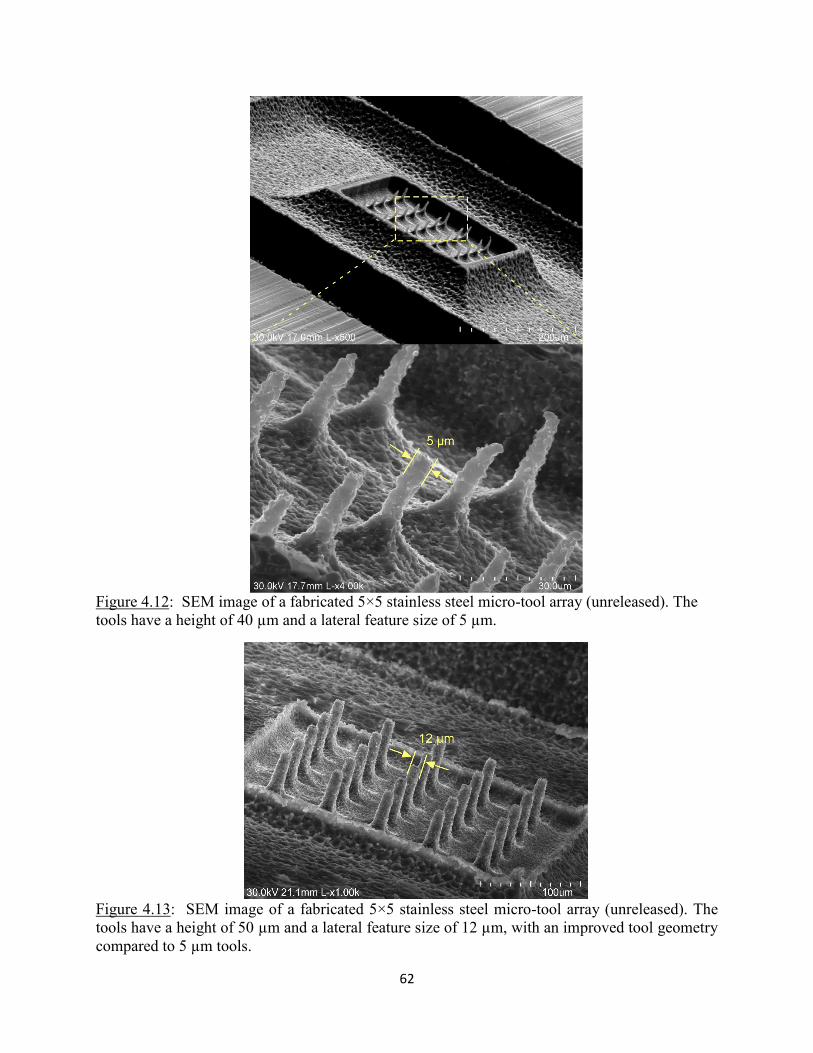
62


tools have a height of 40 µm and a lateral feature size of 5 µm.


tools have a height of 50 µm and a lateral feature size of 12 µm, with an improved tool geometry

compared to 5 µm tools.

63

4.3.4 Machining results

Batch-mode µUSM using workpiece vibration was demonstrated using the micro-tool array

described in the previous section. The machining rate (MR) and surface roughness (Sa)

dependence on the workpiece vibration amplitude was evaluated. The dependence of vibration

amplitude on the PZT transducer actuation voltage follows a linear function as described in

Figure 4.4. The micro-tool array was positioned at a starting distance (SD) of 12 µm from the

workpiece and fed at a constant rate of 50 nm/sec. The machining parameters are listed in Table

4.4.

Table 4.4: Machining parameters used in demonstration of batch-mode µUSM using micro-tool

array fabricated by serial µEDM Workpiece Fused silica, flat,

4×4 mm2, 90 µm

thickness

Transducer actuation voltage 10–50 Vp-p

Vibration amplitude range (µm) 0.7–4.0

Transducer actuation freq. 20 kHz

Starting distance (SD) 12 µm

Tool feed rate 50 nm/sec

Machining time 5 mins.

Slurry type WC(100 nm):H20:: 1:1 (by wt.)

Figures 4.14 and 4.15 show the average machining depth and surface roughness, Sa,

dependence on the workpiece vibration amplitude respectively. These were measured using an

interferometer (LEXTTM

, Olympus Corporation, PA, USA). The batch-mode machining resulted

in transfer of a 2×3 array of machined features onto the workpiece. An average of the depth and

roughness, Sa, of all these features was used to represent the depth and Sa of a machined pattern.

The average machined depth of the features ranged from 2–26 µm for different actuation

voltages. The corresponding machining rates ranged from 6–90 nm/sec for different actuation

voltages. The average surface roughness, Sa, was ≈50 nm. The tool wear, i.e. the ratio of the

tool height worn to the machined depth, was <4%.

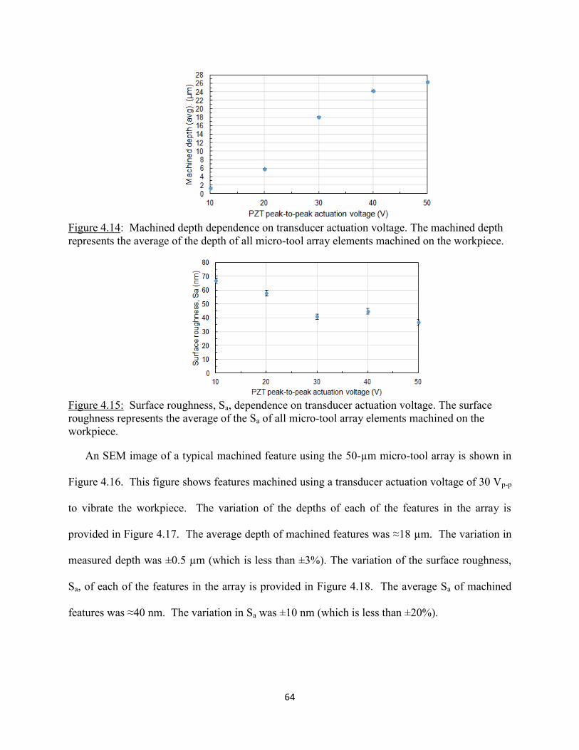
64

Figure 4.14: Machined depth dependence on transducer actuation voltage. The machined depth

represents the average of the depth of all micro-tool array elements machined on the workpiece.

Figure 4.15: Surface roughness, Sa, dependence on transducer actuation voltage. The surface

roughness represents the average of the Sa of all micro-tool array elements machined on the

workpiece.

An SEM image of a typical machined feature using the 50-µm micro-tool array is shown in

Figure 4.16. This figure shows features machined using a transducer actuation voltage of 30 Vp-p

to vibrate the workpiece. The variation of the depths of each of the features in the array is

provided in Figure 4.17. The average depth of machined features was ≈18 µm. The variation in

measured depth was ±0.5 µm (which is less than ±3%). The variation of the surface roughness,

Sa, of each of the features in the array is provided in Figure 4.18. The average Sa of machined

features was ≈40 nm. The variation in Sa was ±10 nm (which is less than ±20%).

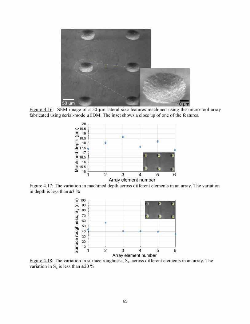
65

Figure 4.16: SEM image of a 50-µm lateral size features machined using the micro-tool array

fabricated using serial-mode µEDM. The inset shows a close up of one of the features.

Figure 4.17: The variation in machined depth across different elements in an array. The variation

in depth is less than ±3 %

Figure 4.18: The variation in surface roughness, Sa, across different elements in an array. The

variation in Sa is less than ±20 %

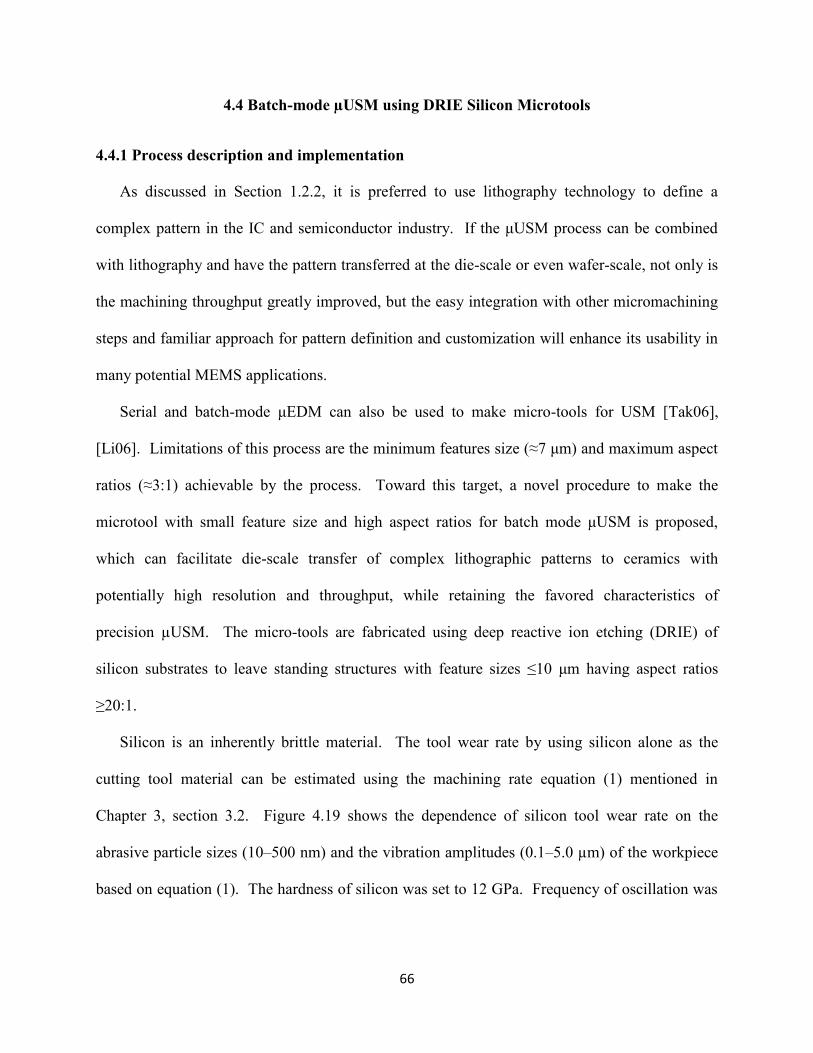
66

4.4 Batch-mode µUSM using DRIE Silicon Microtools

4.4.1 Process description and implementation

As discussed in Section 1.2.2, it is preferred to use lithography technology to define a

complex pattern in the IC and semiconductor industry. If the μUSM process can be combined

with lithography and have the pattern transferred at the die-scale or even wafer-scale, not only is

the machining throughput greatly improved, but the easy integration with other micromachining

steps and familiar approach for pattern definition and customization will enhance its usability in

many potential MEMS applications.

Serial and batch-mode μEDM can also be used to make micro-tools for USM [Tak06],

[Li06]. Limitations of this process are the minimum features size (≈7 μm) and maximum aspect

ratios (≈3:1) achievable by the process. Toward this target, a novel procedure to make the

microtool with small feature size and high aspect ratios for batch mode μUSM is proposed,

which can facilitate die-scale transfer of complex lithographic patterns to ceramics with

potentially high resolution and throughput, while retaining the favored characteristics of

precision µUSM. The micro-tools are fabricated using deep reactive ion etching (DRIE) of

silicon substrates to leave standing structures with feature sizes ≤10 μm having aspect ratios

≥20:1.

Silicon is an inherently brittle material. The tool wear rate by using silicon alone as the

cutting tool material can be estimated using the machining rate equation (1) mentioned in

Chapter 3, section 3.2. Figure 4.19 shows the dependence of silicon tool wear rate on the

abrasive particle sizes (10–500 nm) and the vibration amplitudes (0.1–5.0 µm) of the workpiece

based on equation (1). The hardness of silicon was set to 12 GPa. Frequency of oscillation was

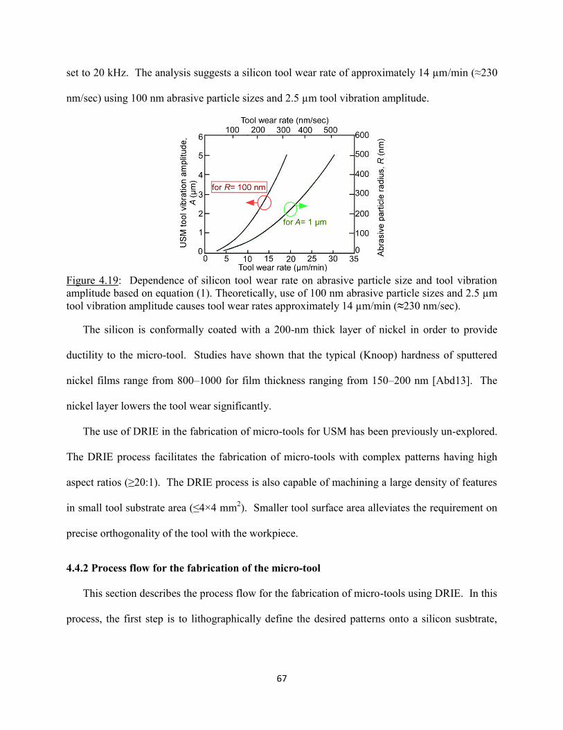
67

set to 20 kHz. The analysis suggests a silicon tool wear rate of approximately 14 µm/min (≈230

nm/sec) using 100 nm abrasive particle sizes and 2.5 µm tool vibration amplitude.

Figure 4.19: Dependence of silicon tool wear rate on abrasive particle size and tool vibration

amplitude based on equation (1). Theoretically, use of 100 nm abrasive particle sizes and 2.5 µm

tool vibration amplitude causes tool wear rates approximately 14 µm/min (≈230 nm/sec).

The silicon is conformally coated with a 200-nm thick layer of nickel in order to provide

ductility to the micro-tool. Studies have shown that the typical (Knoop) hardness of sputtered

nickel films range from 800–1000 for film thickness ranging from 150–200 nm [Abd13]. The

nickel layer lowers the tool wear significantly.

The use of DRIE in the fabrication of micro-tools for USM has been previously un-explored.

The DRIE process facilitates the fabrication of micro-tools with complex patterns having high

aspect ratios (≥20:1). The DRIE process is also capable of machining a large density of features

in small tool substrate area (≤4×4 mm2). Smaller tool surface area alleviates the requirement on

precise orthogonality of the tool with the workpiece.

4.4.2 Process flow for the fabrication of the micro-tool

This section describes the process flow for the fabrication of micro-tools using DRIE. In this

process, the first step is to lithographically define the desired patterns onto a silicon susbtrate,

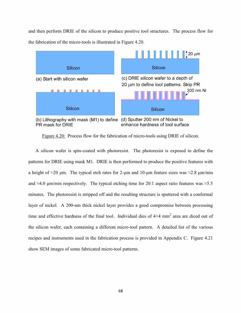
68

and then perform DRIE of the silicon to produce positive tool structures. The process flow for

the fabrication of the micro-tools is illustrated in Figure 4.20.

Figure 4.20: Process flow for the fabrication of micro-tools using DRIE of silicon.

A silicon wafer is spin-coated with photoresist. The photoresist is exposed to define the

patterns for DRIE using mask M1. DRIE is then performed to produce the positive features with

a height of ≈20 μm. The typical etch rates for 2-μm and 10-μm feature sizes was ≈2.8 μm/min

and ≈4.0 μm/min respectively. The typical etching time for 20:1 aspect ratio features was ≈5.5

minutes. The photoresist is stripped off and the resulting structure is sputtered with a conformal

layer of nickel. A 200-nm thick nickel layer provides a good compromise between processing

time and effective hardness of the final tool. Individual dies of 4×4 mm2 area are diced out of

the silicon wafer, each containing a different micro-tool pattern. A detailed list of the various

recipes and instruments used in the fabrication process is provided in Appendix C. Figure 4.21

show SEM images of some fabricated micro-tool patterns.

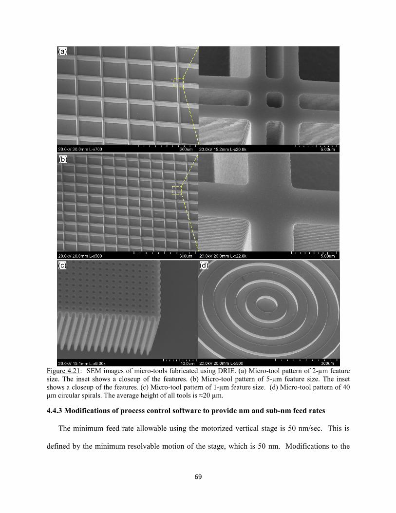
69

Figure 4.21: SEM images of micro-tools fabricated using DRIE. (a) Micro-tool pattern of 2-µm feature

size. The inset shows a closeup of the features. (b) Micro-tool pattern of 5-µm feature size. The inset

shows a closeup of the features. (c) Micro-tool pattern of 1-µm feature size. (d) Micro-tool pattern of 40

µm circular spirals. The average height of all tools is ≈20 µm.

4.4.3 Modifications of process control software to provide nm and sub-nm feed rates

The minimum feed rate allowable using the motorized vertical stage is 50 nm/sec. This is

defined by the minimum resolvable motion of the stage, which is 50 nm. Modifications to the

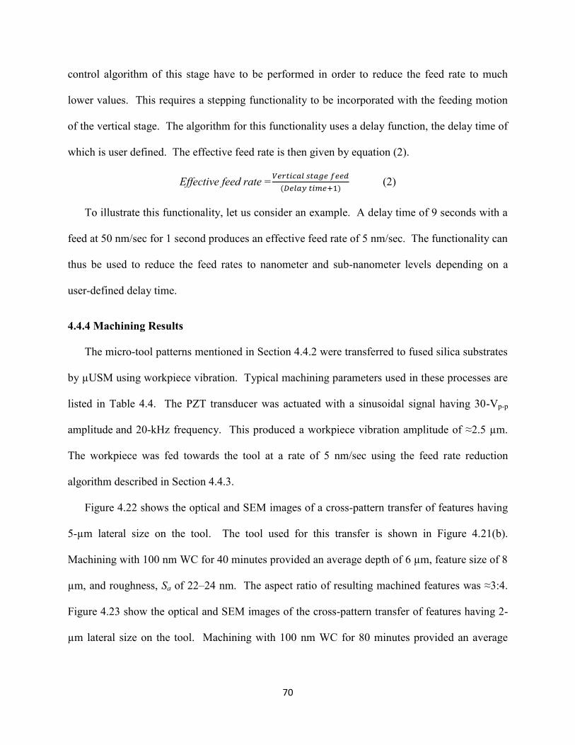
70

control algorithm of this stage have to be performed in order to reduce the feed rate to much

lower values. This requires a stepping functionality to be incorporated with the feeding motion

of the vertical stage. The algorithm for this functionality uses a delay function, the delay time of

which is user defined. The effective feed rate is then given by equation (2).

Effective feed rate =

(2)

To illustrate this functionality, let us consider an example. A delay time of 9 seconds with a

feed at 50 nm/sec for 1 second produces an effective feed rate of 5 nm/sec. The functionality can

thus be used to reduce the feed rates to nanometer and sub-nanometer levels depending on a

user-defined delay time.

4.4.4 Machining Results

The micro-tool patterns mentioned in Section 4.4.2 were transferred to fused silica substrates

by µUSM using workpiece vibration. Typical machining parameters used in these processes are

listed in Table 4.4. The PZT transducer was actuated with a sinusoidal signal having 30-Vp-p

amplitude and 20-kHz frequency. This produced a workpiece vibration amplitude of ≈2.5 µm.

The workpiece was fed towards the tool at a rate of 5 nm/sec using the feed rate reduction

algorithm described in Section 4.4.3.

Figure 4.22 shows the optical and SEM images of a cross-pattern transfer of features having

5-µm lateral size on the tool. The tool used for this transfer is shown in Figure 4.21(b).

Machining with 100 nm WC for 40 minutes provided an average depth of 6 µm, feature size of 8

µm, and roughness, Sa of 22–24 nm. The aspect ratio of resulting machined features was ≈3:4.

Figure 4.23 show the optical and SEM images of the cross-pattern transfer of features having 2-

µm lateral size on the tool. Machining with 100 nm WC for 80 minutes provided an average

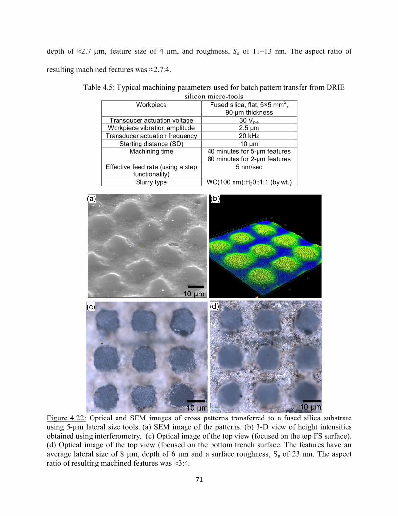
71

depth of ≈2.7 µm, feature size of 4 µm, and roughness, Sa of 11–13 nm. The aspect ratio of

resulting machined features was ≈2.7:4.

Table 4.5: Typical machining parameters used for batch pattern transfer from DRIE

silicon micro-tools Workpiece Fused silica, flat, 5×5 mm

2,

90-µm thickness

Transducer actuation voltage 30 Vp-p

Workpiece vibration amplitude 2.5 µm

Transducer actuation frequency 20 kHz

Starting distance (SD) 10 µm

Machining time 40 minutes for 5-µm features 80 minutes for 2-µm features

Effective feed rate (using a step functionality)

5 nm/sec

Slurry type WC(100 nm):H20::1:1 (by wt.)




(d) Optical image of the top view (focused on the bottom trench surface. The features have an

average lateral size of 8 µm, depth of 6 µm and a surface roughness, Sa of 23 nm. The aspect

ratio of resulting machined features was ≈3:4.

72




(d) Optical image of the top view (focused on the bottom trench surface. The features have an

average lateral size of 4 µm, depth of 2.7 µm and a surface roughness, Sa of 12 nm. The aspect

ratio of resulting machined features was ≈2.7:4.

4.5 Discussion and Conclusions

The vibration of the workpiece in μUSM alleviates slurry precipitation or settling that

presents a challenge for 3-D machining. This eliminates the need for additional mounting

configurations associated with the machining of 3-D microstructures with high aspect ratios

(which was described in Chapter 3, Section 3.4). The workpiece vibration amplitude was

regulated from 1–7 µm by varying the actuation voltage of the piezoelectric PZT transducer.

73

The process was characterized to study the influence of workpiece vibration amplitudes, tool

feeding and machining time on the machining rates and surface roughness. The typical

machining rates ranged from 5–50 nm/sec for vibration levels ranging from 1–8 μm. The

average surface roughness, Sa, was ≈50 nm. The tool wear, i.e. the ratio of the tool height worn

to the machined depth, was <4%. The workpiece vibration agitated the slurry, alleviating slurry

settling.

Batch mode μUSM was demonstrated using SS micro-tool arrays fabricated using serial

μEDM. A 2×3 array of micro cavities was transferred to a ceramic substrate using μUSM with

workpiece vibration. The average depth was 18 μm resulting in aspect ratios of ≈2:5. The

variation in feature sizes of cavities was ≤3%. The variation in depths of cavities was ≤25%.

The tool wear was <4%.

The fabrication of silicon cutting tools using DRIE provides lithographic compatibility in

μUSM, greatly enhancing its throughput. This procedure allows μUSM using cutting tools with

feature sizes ≤5 µm and high aspect ratios (≥20:1). Patterns of 2 and 5 µm were successfully

transferred onto ceramic substrates. The resulting aspect ratios aspect ratios were ≈3:4.

74

CHAPTER 5

Conclusions and Future Work

This chapter provides the summary and conclusions of the research results presented in

previous chapters, as well as the outlines of future work of this research effort.

5.1 Conclusions

This research aimed to address the issue of precision and scalability in μUSM, which is of

interest to a number of MEMS industries. Three primary goals were explored in this effort. The

first goal was to develop a fabrication technology for ultra-high precision machining of hard and

brittle materials such as ceramicsm, which provides high resolution and high surface quality, and

precise control of machining rates. The second goal was to explore a mode of μUSM in which

the workpiece is vibrated and not the tool. The main motivation behind vibrating the workpiece

is to eliminate the settling of slurry particles, which presents a challenge for the machining of 3-

D microstructures. The third goal was to explore the resolution limits of μUSM by using silicon

micromachined tools that were lithographically patterned and fabricated. This would greatly

enhance the throughput of the μUSM process, as well as push the scalability of the machined

features to sub-10 μm levels.

The first step in realizing all the goals set for this work was to identify and evaluate suitable

instrument configurations that would enable precision in μUSM. This required the

customization of a conventional USM system. The customization of the ultrasound generator

components provided a low vibration amplitude of the tool (≤ 7 µm). Low tool vibration

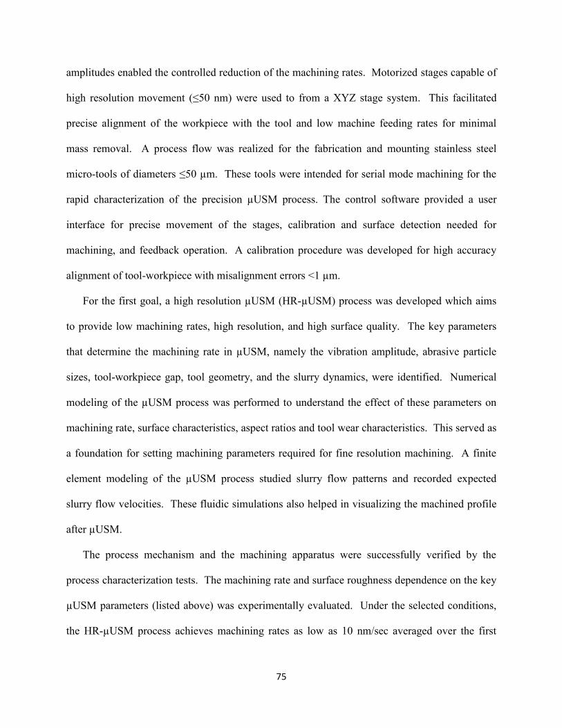
75

amplitudes enabled the controlled reduction of the machining rates. Motorized stages capable of

high resolution movement (≤50 nm) were used to from a XYZ stage system. This facilitated

precise alignment of the workpiece with the tool and low machine feeding rates for minimal

mass removal. A process flow was realized for the fabrication and mounting stainless steel

micro-tools of diameters ≤50 µm. These tools were intended for serial mode machining for the

rapid characterization of the precision µUSM process. The control software provided a user

interface for precise movement of the stages, calibration and surface detection needed for

machining, and feedback operation. A calibration procedure was developed for high accuracy

alignment of tool-workpiece with misalignment errors <1 µm.

For the first goal, a high resolution µUSM (HR-µUSM) process was developed which aims

to provide low machining rates, high resolution, and high surface quality. The key parameters

that determine the machining rate in µUSM, namely the vibration amplitude, abrasive particle

sizes, tool-workpiece gap, tool geometry, and the slurry dynamics, were identified. Numerical

modeling of the µUSM process was performed to understand the effect of these parameters on

machining rate, surface characteristics, aspect ratios and tool wear characteristics. This served as

a foundation for setting machining parameters required for fine resolution machining. A finite

element modeling of the µUSM process studied slurry flow patterns and recorded expected

slurry flow velocities. These fluidic simulations also helped in visualizing the machined profile

after µUSM.

The process mechanism and the machining apparatus were successfully verified by the

process characterization tests. The machining rate and surface roughness dependence on the key

µUSM parameters (listed above) was experimentally evaluated. Under the selected conditions,

the HR-µUSM process achieves machining rates as low as 10 nm/sec averaged over the first

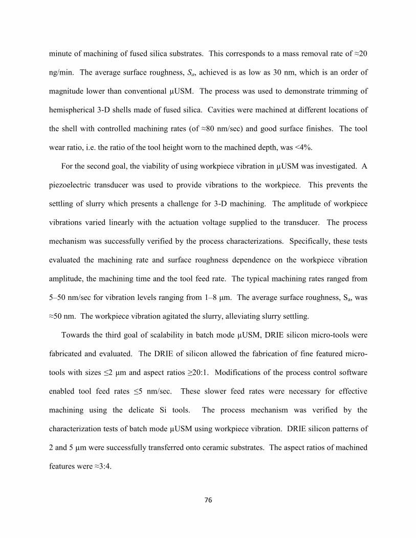
76

minute of machining of fused silica substrates. This corresponds to a mass removal rate of ≈20

ng/min. The average surface roughness, Sa, achieved is as low as 30 nm, which is an order of

magnitude lower than conventional µUSM. The process was used to demonstrate trimming of

hemispherical 3-D shells made of fused silica. Cavities were machined at different locations of

the shell with controlled machining rates (of ≈80 nm/sec) and good surface finishes. The tool

wear ratio, i.e. the ratio of the tool height worn to the machined depth, was <4%.

For the second goal, the viability of using workpiece vibration in µUSM was investigated. A

piezoelectric transducer was used to provide vibrations to the workpiece. This prevents the

settling of slurry which presents a challenge for 3-D machining. The amplitude of workpiece

vibrations varied linearly with the actuation voltage supplied to the transducer. The process

mechanism was successfully verified by the process characterizations. Specifically, these tests

evaluated the machining rate and surface roughness dependence on the workpiece vibration

amplitude, the machining time and the tool feed rate. The typical machining rates ranged from

5–50 nm/sec for vibration levels ranging from 1–8 μm. The average surface roughness, Sa, was

≈50 nm. The workpiece vibration agitated the slurry, alleviating slurry settling.

Towards the third goal of scalability in batch mode µUSM, DRIE silicon micro-tools were

fabricated and evaluated. The DRIE of silicon allowed the fabrication of fine featured micro-

tools with sizes ≤2 μm and aspect ratios ≥20:1. Modifications of the process control software

enabled tool feed rates ≤5 nm/sec. These slower feed rates were necessary for effective

machining using the delicate Si tools. The process mechanism was verified by the

characterization tests of batch mode µUSM using workpiece vibration. DRIE silicon patterns of

2 and 5 µm were successfully transferred onto ceramic substrates. The aspect ratios of machined

features were ≈3:4.

77

Overall, this effort has helped redefine the precision and scalability limits of µUSM. The

machining rates (≤10 nm/sec) and surface finishes (Sa≤30 nm) obtained in this work are

approximately an order of magnitude lower than that achievable using conventional µUSM. The

precision achievable using the fabrication technologies described in this work is beneficial to a

variety of potential MEMS applications and its utility for the trimming 3-D microshells is

demonstrated. The use of workpiece vibration agitated the slurry, alleviating slurry settling. The

developed batch mode µUSM process using DRIE silicon micro-tools pushes the scalability

limits of µUSM by patterning sub-10 µm features, with high throughput.

5.2 Future Work

Several improvements to the precision µUSM process can be envisioned in order to improve

the process efficiency.

Use of AE feedback mode of operation

In this effort, the process control used a simple algorithm for feedback machining mode

(Figure 2.7 and Appendix B.1). The algorithm monitors the acoustic emission (AE) signal level

and regulates the tool feed rate. The tool feed rate is reduced if the acoustic emission signal

crosses a threshold value, which occurs due to the close proximity of the tool to the workpiece.

This threshold value is user defined and is based on statistical measurements. Unfortunately, the

AE sensor signal (and the ideal threshold value) for machine feeding is a function of various

factors other than the tool proximity, such as the slurry concentrations, debris accumulation, etc.

and varies across machining cycles. A user defined threshold does not accurately reflect the tool

proximity alone during µUSM operation.

The threshold level variation is not a significant issue for detection of an impulse, such as

that used in the calibration for tool touch off with the workpiece. The impulse signal measured

78

when the tool makes physical contact with the workpiece is one that is orders of magnitude

larger than the threshold, enabling easier detection. During machining, however, the tool

remains in close proximity of the workpiece, resulting in an AE signal which is relatively closer

to the threshold value. Slight variations in this signal can then cause unwanted shifts in

machining feed rates, lowering the efficiency of the process.

To this end, a more sophisticated control algorithm is needed for realtime time adjustment of

the threshold parameter in feedback. This algorithm should be capable of mapping various

environmental conditions and automatic adjustment of feedback thresholds. An automated

threshold adjustment would not only enhance the machining efficiency in terms of rates and

surface finishes, but would also contribute to better tool life.

Use of a hyrdrophobic coating during machining

The accuracy of machining may potentially be further improved by masking the surface of

the workpiece with a hydrophobic material. Hydrophobic materials can be selectively coated on

the workpiece to define regions that are not to be attacked by the water based slurry. This may

provide selectivity during the machining process to avoid any unwanted machining as a result of

the vortex nature of the slurry flow. As a result, the edge definition of the resulting features may

be enhanced.

Post fabrication, batch mode trimming of MEMS devices

A batch mode process can be envisioned for the post fabrication trimming of devices that

have been lithographically patterned and fabricated. For example, arrays of 3-D MEMS

resonators, timing references, and inertial sensors, such as those described in the introduction of

Chapter 3, can be trimmed in batch mode to reduce and device asymmetry that is common across

devices. A ‘trimming template’ can be prepared using DRIE for use as a cutting tool for

79

ultrasonic machining based trimming. The salient features of the HR-µUSM process (described

in Chapter 3), i.e. low machining rates (≤10 nm/sec) and superior surface roughness (Sa≤30 nm),

can then be used for precision mass removal of these MEMS devices. A batch mode trimming

operation will greatly enhance the throughput of the trimming process and would be beneficial to

a variety of MEMS industries. This is worthy of future research.

80

APPENDICES

APPENDIX A

Metglas- Elgiloy magnetoelastic sensors fabricated using µEDM

A.1 Overview

The fabrication of 3D structures with feature sizes <1 µm is possible using µEDM [Tak02].

For example, serial and batch manufacturing of cardiac stents has been demonstrated in [Tak06,

Tak04]. While the fabrication of structures with complex shapes and small features sizes using

µEDM has been demonstrated before, the integration of these structures to form a

sensor/actuator faces certain challenges. This section addresses certain process integration

challenges of µEDM. As an illustrative example, Metglas-Elgiloy stent cell resonators are

fabricated using µEDM and their application to viscosity and mass sensing is explored [Vis13].

These magnetoelastic sensors integrated with a stent can be used to wirelessly monitor restenosis

in a peripheral artery stents [Vis13]. The sensors are fabricated from 28 μm thick foils of

magnetoelastic 2826MB MetglasTM

, an amorphous Ni-Fe alloy. A gold-indium eutectic bonding

process is used to bond MetglasTM

and Elgiloy foils, which are subsequently patterned using

µEDM to form bi-layer resonators. The response of the sensor to viscosity changes and mass

loading that precede and accompany artery occlusion is tested in vitro. This effort aims to

address some of the challenges in the µEDM of structures and subsequent integration to form a

sensor.

81

A.2 Sensor design

As shown in Figure A.1, the sensor design conforms to the cell of a conventional stent

structure. The stent design follows a wishbone-array pattern that is favored for its flexibility

during expansion. The dimensions of the stent cell and the sensor active area are shown in Fig.

A.1. The sensor layer comprises a frame and an active resonator portion. The frame consists of

150 µm wide struts that are patterned in the same wishbone-array pattern as a 12 mm × 1.46 mm

stent cell. The frame is bonded to the stent struts. The active portion is a 10 mm long symmetric

leaf shape and is connected to the frame with a small anchor at mid-length. The leaf shape nests

within the frame and stent cell, with a uniform gap separating the active portion from the frame.

This gap is 125 µm wide and allows for mechanical decoupling between the sensor and the

frame. The typical active area of a sensor is approximately 4.5 mm2. The resonator is excited in

its fundamental, longitudinal extensional mode of vibration which produces movement of the

ends of the active area of the sensor.

Figure A.1: Sensor and stent geometry showing important dimensions. A sensor bonded to a

single stent cell is also shown.

The stent application calls for a generally tubular shape for use in angioplasty. This sensor

design allows for the easy coiling of stents into this shape without excessive mechanical strain on

the magnetoelastic material, which may lead to unwanted shifts in resonance response.

82

A.3 Sensor fabrication and process integration

The process flow for the fabrication of bi-layer stent cell resonators integrated with the stent

is shown in Figure A.2 (this process is intended to provide rapid prototyping for research

investigations and will need to be modified for final production). MetglasTM

2826MB and

Elgiloy foils are aligned and bonded using the Au-In eutectic bonding process [Lee93]. This

results in bi-layer foils comprising the sensor and stent material.

Figure A.2: Process flow for the fabrication of bi-layer stent cell resonators integrated with the

stent. (1) MetglasTM

2826MB and Elgiloy foils are aligned and bonded using the Au-In eutectic

bonding process to form the bi-layer. (2) Batch patterning of the bonded foils is performed using

µ-EDM. (3) Bi-layer stent cell resonators at specific locations along the stent frame are

fabricated. Parylene deposition is then performed on the resonators to passivate them and make

them bio-compatible.

Isolated, single stent cell resonators are patterned from a pre-bonded MetglasTM

2826MB to

Elgiloy piece. Batch patterning of these resonators is carried out by serial micro-electrode

83

discharge machining (µEDM) of pre-bonded MetglasTM

to Elgiloy pieces. Tungsten tool

electrodes of 125 µm diameter provide a good compromise between machining speed and

minimum feature sizes achievable and were thus used in the µEDM process. The machined

sensors are released and cleaned thoroughly to remove any debris as a result of the machining.

The resulting single stent cell resonators are bi-layers of MetglasTM

2826MB and Elgiloy. A

fabricated, isolated, single stent-cell, bi-layer resonator is shown in Figure A.3.

Figure A.3: Fabricated resonators using µEDM (a) Isolated sensor comprising of bi-layer

MetglasTM

-Elgiloy resonators. (b) Perspective view of the anchor of the bi-layer resonators.

Magnetoelastic alloys are known to corrode in aqueous environments due to its high iron

content. To passivate the material, the sensors are coated in a conformal layer of 200 nm thick

Parylene-C using a standard vacuum deposition technique. This process results in sensors that

are more robust in corrosive environments while causing negligible shifts in resonator frequency

and amplitude response.

A.4 Experimental testing and results

Isolated sensors were tested in vitro for resonance response to various parameter changes.

The unloaded response of a typical sensor in air is presented in Figure A.4. For this device, the

typical unloaded resonant frequency is 361 kHz for the fundamental, longitudinal mode of

vibration. The sensitivity was evaluated for changes in flow velocity of water. The flow

velocity was varied between 20 cm/sec and 11 cm/sec to mimic systolic and diastolic conditions

84

of blood flow. The measured frequency response for each condition, at 37°C, is shown in Figure

A.5. The maximum increase in resonant frequency, due to 9 cm/sec decrease in flow velocity,

fell within the measurement error of the network analyzer. The measured sensitivity of the

fabricated sensors to flow velocity was less than 155 ppm/cm.s-1

. This is a favorable attribute

because the sensors are not intended to respond to flow velocity.

Figure A.4: Frequency response of unloaded sensor in air. The measured resonant frequency is

361 kHz while the custom magnetomechanical FEA model resonates at 346 kHz.

Figure A.5: Measured resonance plots of bi-layer resonators in flow at 37°C. Diastolic (flow

velocity of 20 cm/sec) observed fres=356.5 kHz while systolic (flow velocity of 11cm/sec)

observed fres=356.6 kHz.

The typical viscosity sensitivity of the sensors to varying viscosity levels of sugar water flow

is presented in Figure A.6. The resonant frequencies measured are normalized to the unloaded,

sensor resonant frequency in air. For viscosity levels of 1.084 cP and 8.596 cP, the measured

resonant frequency was 357.65 KHz and 356.505 KHz respectively. The maximum change in

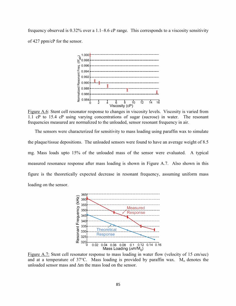
85

frequency observed is 0.32% over a 1.1–8.6 cP range. This corresponds to a viscosity sensitivity

of 427 ppm/cP for the sensor.

Figure A.6: Stent cell resonator response to changes in viscosity levels. Viscosity is varied from

1.1 cP to 15.4 cP using varying concentrations of sugar (sucrose) in water. The resonant

frequencies measured are normalized to the unloaded, sensor resonant frequency in air.

The sensors were characterized for sensitivity to mass loading using paraffin wax to simulate

the plaque/tissue depositions. The unloaded sensors were found to have an average weight of 8.5

mg. Mass loads upto 15% of the unloaded mass of the sensor were evaluated. A typical

measured resonance response after mass loading is shown in Figure A.7. Also shown in this

figure is the theoretically expected decrease in resonant frequency, assuming uniform mass

loading on the sensor.

Figure A.7: Stent cell resonator response to mass loading in water flow (velocity of 15 cm/sec)

and at a temperature of 37°C. Mass loading is provided by paraffin wax. Mo denotes the

unloaded sensor mass and ∆m the mass load on the sensor.

86

The measured sensitivity to mass loading was found to range from 63000 to 65000 ppm/mg

with a maximum resonant frequency change of 8.1% for 15% mass loading on the sensors.

Additionally, the trend observed in measured response agrees with that seen in the theoretical

response within 3.5% error.

An assessment of repeatability involved resonance measurements for 15 trials with a time

interval of 10 minutes in between trials with the sensor position and interrogation parameters

maintained constant for all trials. The maximum change in resonant frequency measured

between trials was around 0.01% or 100 ppm over a time period of 140 minutes. This

corresponds to a mass load of 0.02% of the unloaded sensors mass.

A.5 Conclusion

The fabrication of a magnetoelastic sensor using µEDM, intended for the wireless monitoring

of restenosis, has been presented. The isolated sensors used in these work are made of Metglas-

Elgiloy bi-layers. The metglas serves as the sensor material while the elgiloy is the stent

material. µEDM is used for the patterning of these bi-layers into sensor shapes that conform

with that of a conventional stent cell. The minimum feature sizes used in this work are as low as

125 µm and are designed for stent applications. However, the capabilities of µEDM allow the

fabrication of features with sizes as small as 5 µm. This opens up the possibility of microscale

sensors and actuators that can be fabricated using µEDM which may be used for a wide variety

of applications.

87

APPENDIX B

B.1 Program Script of Process Control Software for the Precision μUSM Apparatus

Imports System Imports System.Text Imports System.Threading Imports System.Runtime.InteropServices Imports PI Imports NationalInstruments.DAQmx Public Class AEFeedbackStageControl Public Declare Function GetCurrentThreadId Lib "kernel32" () As Long 'NI-DAQmx variables Public taskhandle As Long ' NI DAQ Task Handler Public TaskIsRunning As Boolean ' NI DAQ Task running flag Public ScaledData() As Double ' Scaled Data Array from NI DAQ ' Other Global Variables Public AvgForce As Double ' statistic sensor data Public MaxForce As Double Public RMS_AE(513) As Double Public RMS_Counter As Integer Public STD_Counter As Integer Public MaxAE As Double Public AvgData As Double Public SumData As Double Public SumDataAvg As Double Public MaxData As Double Public FFTRealOut(1024) As Double, FFTImgIn(1024) As Double, FFTImgOut(1024) As Double Public FFTData(513) As Double Public Const CalSpeed = 0.005 ' Calibration feeding speed Public Const InitSpeed = 0.0005 ' initial feeding speed Public CurrentSpeed As Single ' current feeding speed Public Const CuttingThreshold = 0.5 ' threshold value for machining starting point Public t_start As Double ' machining starting timer value Public t_end As Double ' machining ending timer value Public t_elapse As Double ' machining time Public t_buffer As Double ' machining time buffer Public t_display As Double ' machining time buffer Public en_counttime ' Time counter state control flag Public flag_cal As Boolean ' Flag to choose calibration or machining feeding Public flag_feedback As Boolean ' Flag to choose force feedback feeding or constant speed feeding Public zeropos(1) As Double ' zero position of tool head Public currentpos(1) As Double ' current position of tool head Public currentCutDepth As Double ' Current cutting depth 'Public inc_timer As Double Dim constSpdVelocity(1) As Double Dim i As Integer Dim icounter As Integer Dim sbErrorMessage As New StringBuilder(1024) Dim sbAxes As New StringBuilder(1024) Dim sAxes As String Dim iReturn(3) As Integer Dim iControllerReady As Integer Dim sbReturn As New StringBuilder(1024)

88

Dim sbHeader As New StringBuilder(1024) Dim iError As Long Dim iChnl(3) As Integer Dim iVal(3) As Integer Dim bFlags(3) As Integer Dim iDataRecorderOptions(3) As Integer Dim dTarget(1) As Double Dim dVelocity(1) As Double Dim dPosition(1) As Double Dim dPosLimit(1) As Double Dim dNegLimit(1) As Double Dim dDataTable(2000) As Double Dim wd_inmm As Double Dim bMoving(1) As Integer Private IDs(16) As Long 'Private p_iControllerId ' Form-wide NI-DAQmx variables Private myTask As Task 'Main Task which is Assigned when a Button is Clicked Private myTask1 As Task 'Main Task which is Assigned when a Button is Clicked Const MinVoltage = -10.0# Const MaxVoltage = 10.0# Const SamplingRate = 200000.0# Const SamplesPerChanlToAcquire = 1024 Const Channel As String = "Dev1/ai0" Public runningTask As Task Private analogInReader As AnalogMultiChannelReader Private analogInReader1 As AnalogMultiChannelReader Private analogCallback As AsyncCallback Private data_everyN_2D(,) As Double Private data_everyN() As Double Private Sub AEFeedbackStageControl_Load(sender As Object, e As EventArgs) Handles MyBase.Load ' Initialize combo box choices ' Setting the Working Distance choices for calibration With comboWD For i = -25 To 150 Step 5 comboWD.Items.Add(i) Next i End With ' Setting the speed choices for constant machining With comboTargetSpd comboTargetSpd.Items.Add(0.0) comboTargetSpd.Items.Add(0.05) comboTargetSpd.Items.Add(0.08) comboTargetSpd.Items.Add(0.1) comboTargetSpd.Items.Add(0.2) comboTargetSpd.Items.Add(0.3) comboTargetSpd.Items.Add(0.4) comboTargetSpd.Items.Add(0.5) comboTargetSpd.Items.Add(0.6) comboTargetSpd.Items.Add(0.8) comboTargetSpd.Items.Add(0.0#) comboTargetSpd.Items.Add(0.5) comboTargetSpd.Items.Add(2.0#) comboTargetSpd.Items.Add(200.0#) End With 'comboTargetSpd.TabIndex = 5 ' Setting target AE RMS feedback value With comboTargetAERMS For i = 1.0# To 8.0# Step 1 comboTargetAERMS.Items.Add(i) Next i End With

89

' Initialize parameters TaskIsRunning = False flag_cal = True flag_feedback = False RMS_Counter = -1 STD_Counter = -1 currentpos(0) = 0 currentpos(1) = 0 For i = 0 To 512 'FFTImgIn(i) = 0 RMS_AE(i) = 0 Next For i = 513 To 1023 'FFTImgIn(i) = 0 Next icounter = 0 ' Initialize the data values End Sub '// STage initialization functionality: Switches on the servo mode of the stages for closed loop operation // Private Sub cmd_StageInit_Click(sender As Object, e As EventArgs) Handles cmd_StageInit.Click '// For the X axis stage: // Me.txtDisplay.Text = Me.txtDisplay.Text + "> SAI?: " If GCS2.qSAI(IDs(0), sbAxes, 1024) = 0 Then iError = GCS2.GetError(IDs(0)) GCS2.TranslateError(iError, sbErrorMessage, 1024) MsgBox(sbErrorMessage.ToString(), , "SAI?") Exit Sub End If sAxes = sbAxes.ToString() Me.txtDisplay.Text = Me.txtDisplay.Text + AddLinefeedToCarrageReturn(sAxes) '// Use only the first axis 'sAxes = "1" '// close the servo loop (closed-loop). // '// Switch on the Servo for all axes bFlags(0) = 1 '// servo on for the axis in the string 'axes'. '// call the SerVO mode command. Me.txtDisplay.Text = Me.txtDisplay.Text + "> SVO 1 1" + vbCrLf If GCS2.SVO(IDs(0), sAxes, bFlags) = 0 Then iError = GCS2.GetError(IDs(0)) GCS2.TranslateError(iError, sbErrorMessage, 1024) MsgBox(sbErrorMessage.ToString(), , "SVO") Exit Sub End If '// confirm servo loop (closed-loop). // '// Check Servo State for all axes Me.txtDisplay.Text = Me.txtDisplay.Text + "> SVO? 1: " If GCS2.qSVO(IDs(0), sAxes, iReturn) = 0 Then iError = GCS2.GetError(IDs(0)) GCS2.TranslateError(iError, sbErrorMessage, 1024) MsgBox(sbErrorMessage.ToString(), , "SVO?") 9: Exit Sub End If Me.txtDisplay.Text = Me.txtDisplay.Text + AddLinefeedToCarrageReturn(iReturn(0)) + vbCrLf '// For the Y axis stage: // '// Get the name of the connected axis. // Me.txtDisplay.Text = Me.txtDisplay.Text + "> SAI?: " If GCS2.qSAI(IDs(1), sbAxes, 1024) = 0 Then iError = GCS2.GetError(IDs(1))

90

GCS2.TranslateError(iError, sbErrorMessage, 1024) MsgBox(sbErrorMessage.ToString(), , "SAI?") Exit Sub End If sAxes = sbAxes.ToString() Me.txtDisplay.Text = Me.txtDisplay.Text + AddLinefeedToCarrageReturn(sAxes) '// Use only the first axis sAxes = "1" '// close the servo loop (closed-loop). // '// Switch on the Servo for all axes bFlags(0) = 1 '// servo on for the axis in the string 'axes'. '// call the SerVO mode command. Me.txtDisplay.Text = Me.txtDisplay.Text + "> SVO 1 1" + vbCrLf If GCS2.SVO(IDs(1), sAxes, bFlags) = 0 Then iError = GCS2.GetError(IDs(1)) GCS2.TranslateError(iError, sbErrorMessage, 1024) MsgBox(sbErrorMessage.ToString(), , "SVO") Exit Sub End If '// confirm servo loop (closed-loop). // '// Check Servo State for all axes Me.txtDisplay.Text = Me.txtDisplay.Text + "> SVO? 1: " If GCS2.qSVO(IDs(1), sAxes, iReturn) = 0 Then iError = GCS2.GetError(IDs(1)) GCS2.TranslateError(iError, sbErrorMessage, 1024) MsgBox(sbErrorMessage.ToString(), , "SVO?") Exit Sub End If Me.txtDisplay.Text = Me.txtDisplay.Text + AddLinefeedToCarrageReturn(iReturn(0)) + vbCrLf '// For the Z axis stage: // '// Get the name of the connected axis. // Me.txtDisplay.Text = Me.txtDisplay.Text + "> SAI?: " If GCS2.qSAI(IDs(2), sbAxes, 1024) = 0 Then iError = GCS2.GetError(IDs(2)) GCS2.TranslateError(iError, sbErrorMessage, 1024) MsgBox(sbErrorMessage.ToString(), , "SAI?") Exit Sub End If sAxes = sbAxes.ToString() Me.txtDisplay.Text = Me.txtDisplay.Text + AddLinefeedToCarrageReturn(sAxes) ' Use only the first axis sAxes = "1" '// close the servo loop (closed-loop). // '// Switch on the Servo for all axes bFlags(0) = 1 '// servo on for the axis in the string 'axes'. '// call the SerVO mode command. Me.txtDisplay.Text = Me.txtDisplay.Text + "> SVO 1 1" + vbCrLf If GCS2.SVO(IDs(2), sAxes, bFlags) = 0 Then iError = GCS2.GetError(IDs(2)) GCS2.TranslateError(iError, sbErrorMessage, 1024) MsgBox(sbErrorMessage.ToString(), , "SVO") Exit Sub End If '// confirm servo loop (closed-loop). //

91

'// Check Servo State for all axes Me.txtDisplay.Text = Me.txtDisplay.Text + "> SVO? 1: " If GCS2.qSVO(IDs(2), sAxes, iReturn) = 0 Then iError = GCS2.GetError(IDs(2)) GCS2.TranslateError(iError, sbErrorMessage, 1024) MsgBox(sbErrorMessage.ToString(), , "SVO?") Exit Sub End If Me.txtDisplay.Text = Me.txtDisplay.Text + AddLinefeedToCarrageReturn(iReturn(0)) + vbCrLf End Sub '// Homing all the axis : X Y and Z referencing. X and Y to middle reference point and Z to the negative (lowest) reference point // Private Sub cmd_HomeAll_Click(sender As Object, e As EventArgs) Handles cmd_HomeAll.Click 'X referencing to the middle position Me.txtDisplay.Text = Me.txtDisplay.Text + "> FRF 1" + vbCrLf If GCS2.FRF(IDs(0), sAxes) = 0 Then iError = GCS2.GetError(IDs(0)) GCS2.TranslateError(iError, sbErrorMessage, 1024) MsgBox(sbErrorMessage.ToString(), , "FRL") Exit Sub End If Me.txtDisplay.Text = Me.txtDisplay.Text + "Waiting for Referencing..." + vbCrLf If GCS2.IsControllerReady(IDs(0), iControllerReady) = 0 Then MsgBox("Error") End If iControllerReady = 0 While iControllerReady = 0 Application.DoEvents() GCS2.IsControllerReady(IDs(0), iControllerReady) End While Me.txtDisplay.Text = Me.txtDisplay.Text + "Referenced." + vbCrLf 'Y referencing to the middle position Me.txtDisplay.Text = Me.txtDisplay.Text + "> FRF 1" + vbCrLf 'If GCS2.FRF(IDs(1) + 1, sAxes) = 0 Then If GCS2.FRF(IDs(1), sAxes) = 0 Then iError = GCS2.GetError(IDs(1)) GCS2.TranslateError(iError, sbErrorMessage, 1024) MsgBox(sbErrorMessage.ToString(), , "FRL") Exit Sub End If Me.txtDisplay.Text = Me.txtDisplay.Text + "Waiting for Referencing..." + vbCrLf If GCS2.IsControllerReady(IDs(1), iControllerReady) = 0 Then MsgBox("Error") End If iControllerReady = 0 While iControllerReady = 0 Application.DoEvents() GCS2.IsControllerReady(IDs(1), iControllerReady) End While Me.txtDisplay.Text = Me.txtDisplay.Text + "Referenced." + vbCrLf 'Z referencing to the lowest (negative limit) position

92

' default referencing velocity set to 0.5 m/s dVelocity(0) = 0.5 GCS2.VEL(IDs(2), sAxes, dVelocity) Me.txtDisplay.Text = Me.txtDisplay.Text + "> FNL 1" + vbCrLf If GCS2.FNL(IDs(2), sAxes) = 0 Then iError = GCS2.GetError(IDs(2)) GCS2.TranslateError(iError, sbErrorMessage, 1024) MsgBox(sbErrorMessage.ToString(), , "FNL") Exit Sub End If Me.txtDisplay.Text = Me.txtDisplay.Text + "Waiting for Referencing..." + vbCrLf If GCS2.IsControllerReady(IDs(2), iControllerReady) = 0 Then MsgBox("Error") End If iControllerReady = 0 While iControllerReady = 0 Application.DoEvents() GCS2.IsControllerReady(IDs(2), iControllerReady) End While Me.txtDisplay.Text = Me.txtDisplay.Text + "Referenced." + vbCrLf End Sub '// X Axis referencing (Set the Middle position reference as default) Private Sub X_reference_Click(sender As Object, e As EventArgs) Handles X_reference.Click '// Refernce the device. (Reference Switch) // Me.txtDisplay.Text = Me.txtDisplay.Text + "> FRF 1" + vbCrLf If GCS2.FRF(IDs(0), sAxes) = 0 Then iError = GCS2.GetError(IDs(0)) GCS2.TranslateError(iError, sbErrorMessage, 1024) MsgBox(sbErrorMessage.ToString(), , "FRL") Exit Sub End If Me.txtDisplay.Text = Me.txtDisplay.Text + "Waiting for Referencing..." + vbCrLf If GCS2.IsControllerReady(IDs(0), iControllerReady) = 0 Then MsgBox("Error") End If iControllerReady = 0 While iControllerReady = 0 Application.DoEvents() GCS2.IsControllerReady(IDs(0), iControllerReady) End While Me.txtDisplay.Text = Me.txtDisplay.Text + "Referenced." + vbCrLf End Sub Private Sub XHighSpdChecked_CheckedChanged(sender As Object, e As EventArgs) Handles XHighSpdChecked.CheckedChanged dVelocity(0) = 1.2 GCS2.VEL(IDs(0), sAxes, dVelocity) End Sub Private Sub XLowSpeedChecked_CheckedChanged(sender As Object, e As EventArgs) Handles XLowSpeedChecked.CheckedChanged dVelocity(0) = 0.5 GCS2.VEL(IDs(0), sAxes, dVelocity) End Sub Private Sub XLow2SpeedChecked_CheckedChanged(sender As Object, e As EventArgs) Handles XLow2SpeedChecked.CheckedChanged dVelocity(0) = 0.02 GCS2.VEL(IDs(0), sAxes, dVelocity) End Sub '// X axis Jogging to the left side

93

Private Sub XLeftJog_Click(ByVal sender As System.Object, ByVal e As System.EventArgs) Handles XLeftJog.Click '// command relative motion dTarget(0) = 0 Me.txtDisplay.Text = Me.txtDisplay.Text + "> MOV 1 2" + vbCrLf If GCS2.MOV(IDs(0), sAxes, dTarget) = 0 Then iError = GCS2.GetError(IDs(0)) GCS2.TranslateError(iError, sbErrorMessage, 1024) MsgBox(sbErrorMessage.ToString(), , "MOV") Exit Sub End If bMoving(0) = 1 While (bMoving(0)) GCS2.IsMoving(IDs(0), sAxes, bMoving) Application.DoEvents() End While '// Display position Me.txtDisplay.Text = Me.txtDisplay.Text + "> POS? 1: " If GCS2.qPOS(IDs(0), sAxes, dPosition) = 0 Then iError = GCS2.GetError(IDs(0)) GCS2.TranslateError(iError, sbErrorMessage, 1024) MsgBox(sbErrorMessage.ToString(), , "POS?") Exit Sub End If Me.txtDisplay.Text = Me.txtDisplay.Text + AddLinefeedToCarrageReturn(dPosition(0)) End Sub '// X axis Jogging to the Right side Private Sub XRightJog_Click(sender As Object, e As EventArgs) Handles XRightJog.Click '// command relative motion dTarget(0) = 50 Me.txtDisplay.Text = Me.txtDisplay.Text + "> MOV 1 2" + vbCrLf If GCS2.MOV(IDs(0), sAxes, dTarget) = 0 Then iError = GCS2.GetError(IDs(0)) GCS2.TranslateError(iError, sbErrorMessage, 1024) MsgBox(sbErrorMessage.ToString(), , "MOV") Exit Sub End If bMoving(0) = 1 While (bMoving(0)) GCS2.IsMoving(IDs(0), sAxes, bMoving) Application.DoEvents() End While '// Display position Me.txtDisplay.Text = Me.txtDisplay.Text + "> POS? 1: " If GCS2.qPOS(IDs(0), sAxes, dPosition) = 0 Then iError = GCS2.GetError(IDs(0)) GCS2.TranslateError(iError, sbErrorMessage, 1024) MsgBox(sbErrorMessage.ToString(), , "POS?") Exit Sub End If Me.txtDisplay.Text = Me.txtDisplay.Text + AddLinefeedToCarrageReturn(dPosition(0)) End Sub '// Halts Right of Left jogging when button is clicked Private Sub XJogStop_Click(sender As Object, e As EventArgs) Handles XJogStop.Click GCS2.HLT(IDs(0), sAxes) '// Display position Me.txtDisplay.Text = Me.txtDisplay.Text + "> POS? 1: "

94

If GCS2.qPOS(IDs(0), sAxes, dPosition) = 0 Then iError = GCS2.GetError(IDs(0)) GCS2.TranslateError(iError, sbErrorMessage, 1024) MsgBox(sbErrorMessage.ToString(), , "POS?") Exit Sub End If End Sub '// Y Axis //// '// Y Axis referencing (Set the Middle position reference as default) Private Sub Y_reference_Click(sender As Object, e As EventArgs) Handles Y_reference.Click '// Refernce the device. (Reference Switch) // Me.txtDisplay.Text = Me.txtDisplay.Text + "> FRF 1" + vbCrLf 'If GCS2.FRF(IDs(1) + 1, sAxes) = 0 Then If GCS2.FRF(IDs(1), sAxes) = 0 Then iError = GCS2.GetError(IDs(1)) GCS2.TranslateError(iError, sbErrorMessage, 1024) MsgBox(sbErrorMessage.ToString(), , "FRL") Exit Sub End If Me.txtDisplay.Text = Me.txtDisplay.Text + "Waiting for Referencing..." + vbCrLf If GCS2.IsControllerReady(IDs(1), iControllerReady) = 0 Then MsgBox("Error") End If iControllerReady = 0 While iControllerReady = 0 Application.DoEvents() GCS2.IsControllerReady(IDs(1), iControllerReady) End While Me.txtDisplay.Text = Me.txtDisplay.Text + "Referenced." + vbCrLf End Sub Private Sub YHighSpdChecked_CheckedChanged(sender As Object, e As EventArgs) Handles YHighSpdChecked.CheckedChanged dVelocity(0) = 1.2 GCS2.VEL(IDs(1), sAxes, dVelocity) End Sub Private Sub YLowSpeedChecked_CheckedChanged(sender As Object, e As EventArgs) Handles YLowSpeedChecked.CheckedChanged dVelocity(0) = 0.5 GCS2.VEL(IDs(1), sAxes, dVelocity) End Sub Private Sub YLow2SpeedChecked_CheckedChanged(sender As Object, e As EventArgs) Handles YLow2SpeedChecked.CheckedChanged dVelocity(0) = 0.02 GCS2.VEL(IDs(1), sAxes, dVelocity) End Sub '// Y axis Jogging to the left side Private Sub YLeftJog_Click(sender As Object, e As EventArgs) Handles YLeftJog.Click '// command relative motion dTarget(0) = 0 Me.txtDisplay.Text = Me.txtDisplay.Text + "> MOV 1 2" + vbCrLf If GCS2.MOV(IDs(1), sAxes, dTarget) = 0 Then iError = GCS2.GetError(IDs(1)) GCS2.TranslateError(iError, sbErrorMessage, 1024) MsgBox(sbErrorMessage.ToString(), , "MOV") Exit Sub End If bMoving(0) = 1 While (bMoving(0))

95

GCS2.IsMoving(IDs(1), sAxes, bMoving) Application.DoEvents() End While '// Display position Me.txtDisplay.Text = Me.txtDisplay.Text + "> POS? 1: " If GCS2.qPOS(IDs(1), sAxes, dPosition) = 0 Then iError = GCS2.GetError(IDs(1)) GCS2.TranslateError(iError, sbErrorMessage, 1024) MsgBox(sbErrorMessage.ToString(), , "POS?") Exit Sub End If Me.txtDisplay.Text = Me.txtDisplay.Text + AddLinefeedToCarrageReturn(dPosition(0)) End Sub '// Y axis Jogging to the Right side Private Sub YRightJog_Click(sender As Object, e As EventArgs) Handles YRightJog.Click '// command relative motion dTarget(0) = 50 Me.txtDisplay.Text = Me.txtDisplay.Text + "> MOV 1 2" + vbCrLf If GCS2.MOV(IDs(1), sAxes, dTarget) = 0 Then iError = GCS2.GetError(IDs(1)) GCS2.TranslateError(iError, sbErrorMessage, 1024) MsgBox(sbErrorMessage.ToString(), , "MOV") Exit Sub End If bMoving(0) = 1 While (bMoving(0)) GCS2.IsMoving(IDs(1), sAxes, bMoving) Application.DoEvents() End While '// Display position Me.txtDisplay.Text = Me.txtDisplay.Text + "> POS? 1: " If GCS2.qPOS(IDs(0), sAxes, dPosition) = 0 Then iError = GCS2.GetError(IDs(1)) GCS2.TranslateError(iError, sbErrorMessage, 1024) MsgBox(sbErrorMessage.ToString(), , "POS?") Exit Sub End If Me.txtDisplay.Text = Me.txtDisplay.Text + AddLinefeedToCarrageReturn(dPosition(0)) End Sub '// Halts Right of Left jogging when button is clicked Private Sub YJogStop_Click(sender As Object, e As EventArgs) Handles YJogStop.Click GCS2.HLT(IDs(1), sAxes) '// Display position Me.txtDisplay.Text = Me.txtDisplay.Text + "> POS? 1: " If GCS2.qPOS(IDs(1), sAxes, dPosition) = 0 Then iError = GCS2.GetError(IDs(1)) GCS2.TranslateError(iError, sbErrorMessage, 1024) MsgBox(sbErrorMessage.ToString(), , "POS?") Exit Sub End If End Sub '// Z Axis : Motorized Stage //// Private Sub Z_reference_Click(sender As Object, e As EventArgs) Handles Z_reference.Click '// Refernce the device. (Reference Switch) // ' default referencing velocity set to 0.5 m/s dVelocity(0) = 0.5

96

GCS2.VEL(IDs(2), sAxes, dVelocity) Me.txtDisplay.Text = Me.txtDisplay.Text + "> FNL 1" + vbCrLf If GCS2.FNL(IDs(2), sAxes) = 0 Then iError = GCS2.GetError(IDs(2)) GCS2.TranslateError(iError, sbErrorMessage, 1024) MsgBox(sbErrorMessage.ToString(), , "FNL") Exit Sub End If Me.txtDisplay.Text = Me.txtDisplay.Text + "Waiting for Referencing..." + vbCrLf If GCS2.IsControllerReady(IDs(2), iControllerReady) = 0 Then MsgBox("Error") End If iControllerReady = 0 While iControllerReady = 0 Application.DoEvents() GCS2.IsControllerReady(IDs(2), iControllerReady) End While Me.txtDisplay.Text = Me.txtDisplay.Text + "Referenced." + vbCrLf End Sub Private Sub ZHighSpdChecked_CheckedChanged(sender As Object, e As EventArgs) Handles ZHighSpdChecked.CheckedChanged dVelocity(0) = 0.5 GCS2.VEL(IDs(2), sAxes, dVelocity) End Sub Private Sub ZLowSpeedChecked_CheckedChanged(sender As Object, e As EventArgs) Handles ZLowSpeedChecked.CheckedChanged dVelocity(0) = 0.1 GCS2.VEL(IDs(2), sAxes, dVelocity) End Sub Private Sub ZLowSpeedChecked2_CheckedChanged(sender As Object, e As EventArgs) Handles ZLowSpeedChecked2.CheckedChanged dVelocity(0) = 0.02 GCS2.VEL(IDs(2), sAxes, dVelocity) End Sub '// Z axis Jogging Upwards Private Sub ZUpJog_Click(sender As Object, e As EventArgs) Handles ZUpJog.Click '// command relative motion dTarget(0) = 12.2 Me.txtDisplay.Text = Me.txtDisplay.Text + "> MOV 1 2" + vbCrLf If GCS2.MOV(IDs(2), sAxes, dTarget) = 0 Then iError = GCS2.GetError(IDs(2)) GCS2.TranslateError(iError, sbErrorMessage, 1024) MsgBox(sbErrorMessage.ToString(), , "MOV") Exit Sub End If bMoving(0) = 1 While (bMoving(0)) GCS2.IsMoving(IDs(2), sAxes, bMoving) Application.DoEvents() End While '// Display position Me.txtDisplay.Text = Me.txtDisplay.Text + "> POS? 1: " If GCS2.qPOS(IDs(2), sAxes, dPosition) = 0 Then iError = GCS2.GetError(IDs(2)) GCS2.TranslateError(iError, sbErrorMessage, 1024) MsgBox(sbErrorMessage.ToString(), , "POS?") Exit Sub End If Me.txtDisplay.Text = Me.txtDisplay.Text + AddLinefeedToCarrageReturn(dPosition(0)) End Sub

97

'// Z axis Jogging Downwards Private Sub ZDownJog_Click(sender As Object, e As EventArgs) Handles ZDownJog.Click '// command relative motion dTarget(0) = 0.2 ' default down moving velocity set to 0.5 m/s dVelocity(0) = 0.5 GCS2.VEL(IDs(2), sAxes, dVelocity) Me.txtDisplay.Text = Me.txtDisplay.Text + "> MOV 1 2" + vbCrLf If GCS2.MOV(IDs(2), sAxes, dTarget) = 0 Then iError = GCS2.GetError(IDs(2)) GCS2.TranslateError(iError, sbErrorMessage, 1024) MsgBox(sbErrorMessage.ToString(), , "MOV") Exit Sub End If bMoving(0) = 1 While (bMoving(0)) GCS2.IsMoving(IDs(2), sAxes, bMoving) Application.DoEvents() End While '// Display position Me.txtDisplay.Text = Me.txtDisplay.Text + "> POS? 1: " If GCS2.qPOS(IDs(2), sAxes, dPosition) = 0 Then iError = GCS2.GetError(IDs(2)) GCS2.TranslateError(iError, sbErrorMessage, 1024) MsgBox(sbErrorMessage.ToString(), , "POS?") Exit Sub End If Me.txtDisplay.Text = Me.txtDisplay.Text + AddLinefeedToCarrageReturn(dPosition(0)) End Sub '// Halts Right or Left jogging when button is clicked Private Sub ZJogStop_Click(sender As Object, e As EventArgs) Handles ZJogStop.Click GCS2.HLT(IDs(2), sAxes) '// Display position Me.txtDisplay.Text = Me.txtDisplay.Text + "> POS? 1: " If GCS2.qPOS(IDs(2), sAxes, dPosition) = 0 Then iError = GCS2.GetError(IDs(2)) GCS2.TranslateError(iError, sbErrorMessage, 1024) MsgBox(sbErrorMessage.ToString(), , "POS?") Exit Sub End If End Sub ''//------------------Code for Having button pressed down functionality---------- 'Private Sub Form_Load() ' Timer1.Interval = 100 ' Timer1.Enabled = False 'End Sub 'Private Sub Image1_MouseDown(Button As Integer, Shift As Integer, X As Single, Y As Single) ' If Button = 1 Then Timer1.Enabled = True 'End Sub 'Private Sub Image1_MouseUp(Button As Integer, Shift As Integer, X As Single, Y As Single) ' If Button = 1 Then Timer1.Enabled = False 'End Sub

98

'Private Sub Timer1_Timer() ' Print "Rewinding..." 'End Sub ' Command for Calibhration in Normal Mode Private Sub cmd_CalibrateNM_Click(sender As Object, e As EventArgs) Handles cmd_CalibrateNM.Click ' '' the "Calibrate" button was clicked ''On Error GoTo ErrorHandler ' '' if the com port has already been opened, send the instruction Me.lblMachineStatus.Text = " Command Calibrate Nm button Clicked!" Me.lblStageMvment.Text = " Z axis MOVING (approaching tool at 5 um/s)" cmd_CalibrateNM.Enabled = False cmd_CalibrateStopNM.Enabled = True flag_cal = True ' '''''' ''DAQmx Configure Code' If runningTask Is Nothing Then Try myTask = New Task() myTask.AIChannels.CreateVoltageChannel(Channel, "", CType(-1, AITerminalConfiguration), MinVoltage, MaxVoltage, AIVoltageUnits.Volts) myTask.Timing.ConfigureSampleClock("", SamplingRate, SampleClockActiveEdge.Rising, SampleQuantityMode.ContinuousSamples, SamplesPerChanlToAcquire * 10000) '' Verify the task myTask.Control(TaskAction.Verify) myTask.EveryNSamplesReadEventInterval = SamplesPerChanlToAcquire runningTask = myTask analogInReader = New AnalogMultiChannelReader(myTask.Stream) AddHandler runningTask.EveryNSamplesRead, AddressOf EveryNSamplesEventHandler ' Prepare the table for Data ' aInitializeDataTable(myTask.AIChannels, dataTable) ''InitializeDataTable(myTask.AIChannels, dataTable) ''acquisitionDataGrid.DataSource = dataTable ReDim data_everyN(SamplesPerChanlToAcquire - 1) runningTask.SynchronizeCallbacks = True myTask.Start() 'Stage Control Code' 'MG17Motor1.SetJogMode(CHAN1_ID, JOG_CONTINUOUS, STOP_PROFILED) 'MG17Motor1.SetJogVelParams(CHAN1_ID, 0, 0.1, CalSpeed) 'MG17Motor1.MoveJog(CHAN1_ID, JOG_FWD) dTarget(0) = 12.2 ' Set calibration speed as calspeed dVelocity(0) = CalSpeed GCS2.VEL(IDs(2), sAxes, dVelocity) Me.txtDisplay.Text = Me.txtDisplay.Text + "> MOV 1 2" + vbCrLf If GCS2.MOV(IDs(2), sAxes, dTarget) = 0 Then 'iError = GCS2.GetError(IDs(2)) 'GCS2.TranslateError(iError, sbErrorMessage, 1024) 'MsgBox(sbErrorMessage.ToString(), , "MOV") 'Exit Sub End If 'bMoving(0) = 1 'While (bMoving(0)) ' GCS2.IsMoving(IDs(2), sAxes, bMoving) ' Application.DoEvents() 'End While '// Display position Me.txtDisplay.Text = Me.txtDisplay.Text + "In cmdCalibrate click: > POS? 1: " If GCS2.qPOS(IDs(2), sAxes, dPosition) = 0 Then iError = GCS2.GetError(IDs(2)) GCS2.TranslateError(iError, sbErrorMessage, 1024)

99

MsgBox(sbErrorMessage.ToString(), , "POS?") Exit Sub End If Me.txtDisplay.Text = Me.txtDisplay.Text + AddLinefeedToCarrageReturn(dPosition(0)) ZUpJog.Enabled = False ZDownJog.Enabled = True ZJogStop.Enabled = True cmd_CSpdStart.Enabled = True cmd_AEFBStart.Enabled = True cmd_CalibrateNM.Enabled = True cmd_CalibrateStopNM.Enabled = True 'If Not (runningTask Is Nothing) Then ' runningTask.Stop() ' runningTask = Nothing ' myTask.Dispose() 'End If Exit Sub Catch exception As DaqException MessageBox.Show(exception.Message) runningTask = Nothing 'stopButton.Enabled = False 'startButton.Enabled = True myTask.Dispose() End Try End If End Sub Private Sub cmd_CalibrateStopNM_Click(sender As Object, e As EventArgs) Handles cmd_CalibrateStopNM.Click ' the "Stop" button for constant speed feeding was clicked, stop the movement 'StopMicroStepFeed() '''''' ' Stop the Z axis Motor GCS2.HLT(IDs(2), sAxes) Me.lblMachineStatus.Text = " Command Calibrate STOP button Clicked!" Me.lblStageMvment.Text = " Z axis IDLE " Me.lblCutStatus.Text = "Status: Idle" Me.lblCurrentSpd.Text = "Current Feed Speed: 0 (um/s)" ZDownJog.Enabled = True ZUpJog.Enabled = True cmd_CalibrateNM.Enabled = True cmd_CalibrateStopNM.Enabled = False cmd_CSpdStart.Enabled = True 'cmdAEFBStart.Enabled = True 'cmdCSpdStart.Enabled = True 'cmdAEFBStop.Enabled = False 'cmdCSpdStop.Enabled = False '''''' flag_cal = True flag_feedback = False '''''' ' Call the NIDAQStopTask module to stop the DAQmx task. If Not (runningTask Is Nothing) Then runningTask.Stop() runningTask = Nothing myTask.Dispose() End If End Sub '//AE FEEDBACK MACHINING OPERATION // '////////////////////////////////////////////////// ' The AE Feedback Machining Start button was clicked Private Sub cmd_AEFBStart_Click(sender As Object, e As EventArgs) Handles cmd_AEFBStart.Click t_elapse = 0 t_buffer = 0

100

en_counttime = False CurrentSpeed = InitSpeed flag_cal = False flag_feedback = True '' DAQ Configuration code: Creating task and channel; setting sampling parameters; and starting task: myTask = New Task() myTask.AIChannels.CreateVoltageChannel(Channel, "", CType(-1, AITerminalConfiguration), MinVoltage, MaxVoltage, AIVoltageUnits.Volts) myTask.Timing.ConfigureSampleClock("", SamplingRate, SampleClockActiveEdge.Rising, SampleQuantityMode.ContinuousSamples, SamplesPerChanlToAcquire * 10000) '' Verify the task myTask.Control(TaskAction.Verify) myTask.EveryNSamplesReadEventInterval = SamplesPerChanlToAcquire runningTask = myTask analogInReader = New AnalogMultiChannelReader(myTask.Stream) AddHandler runningTask.EveryNSamplesRead, AddressOf EveryNSamplesEventHandler ReDim data_everyN(SamplesPerChanlToAcquire - 1) runningTask.SynchronizeCallbacks = True myTask.Start() ' Machining with the desired speeds 'StartMicroStepFeed() ZUpJog.Enabled = False ZDownJog.Enabled = False ZJogStop.Enabled = False cmd_CSpdStart.Enabled = False cmd_AEFBStart.Enabled = False cmd_CalibrateNM.Enabled = False cmd_CalibrateStopNM.Enabled = True cmd_AEFBPause.Enabled = True cmd_AEFBStop.Enabled = True End Sub ' The AE Feedback Machining Pause button was clicked Private Sub cmd_AEFBPause_Click(sender As Object, e As EventArgs) Handles cmd_AEFBPause.Click ' Stops the movement 'StopMicroStepFeed() End Sub ' The AE Feedback Machining Stop button was clicked Private Sub cmd_AEFBStop_Click(sender As Object, e As EventArgs) Handles cmd_AEFBStop.Click ' the "Stop" button for AE feedback feeding was clicked, stop the movement 'StopMicroStepFeed() '''''' Me.lblCutStatus.Text = "Status: Idle" Me.lblCurrentSpd.Text = "Current Feed Speed: 0 (um/s)" '''''' '''''' ZUpJog.Enabled = True ZDownJog.Enabled = True ZJogStop.Enabled = True cmd_CSpdStart.Enabled = True cmd_AEFBStart.Enabled = True cmd_CalibrateNM.Enabled = True cmd_CalibrateStopNM.Enabled = True cmd_AEFBPause.Enabled = True cmd_AEFBStop.Enabled = False flag_cal = True flag_feedback = False ' Call the NIDAQStopTask module to stop the DAQmx task. If Not (runningTask Is Nothing) Then runningTask.Stop()

101

runningTask = Nothing myTask.Dispose() End If End Sub '//CONSTANT SPEED MACHINING OPERATION // '////////////////////////////////////////////////// ' The constant Speed machining start button was clicked Private Sub cmd_CSpdStart_Click(sender As Object, e As EventArgs) Handles cmd_CSpdStart.Click t_elapse = 0 t_buffer = 0 en_counttime = False CurrentSpeed = Val(comboTargetSpd.Text) flag_cal = False flag_feedback = False cmd_CSpdStart.Enabled = False cmd_CSpdStop.Enabled = False cmd_CSpdPause.Enabled = False ' DAQ Configuration code: Creating task and channel; setting sampling parameters; and starting task: If runningTask Is Nothing Then Try myTask = New Task() myTask.AIChannels.CreateVoltageChannel(Channel, "", CType(-1, AITerminalConfiguration), MinVoltage, MaxVoltage, AIVoltageUnits.Volts) myTask.Timing.ConfigureSampleClock("", SamplingRate, SampleClockActiveEdge.Rising, SampleQuantityMode.ContinuousSamples, SamplesPerChanlToAcquire * 10000) '' Verify the task myTask.Control(TaskAction.Verify) myTask.EveryNSamplesReadEventInterval = SamplesPerChanlToAcquire runningTask = myTask analogInReader = New AnalogMultiChannelReader(myTask.Stream) AddHandler runningTask.EveryNSamplesRead, AddressOf EveryNSamplesEventHandler ReDim data_everyN(SamplesPerChanlToAcquire - 1) runningTask.SynchronizeCallbacks = True myTask.Start() 'Machining with the desired speeds 'StartMicroStepFeed() 'Setting the speed of the machining constSpdVelocity(0) = CSng(Val(Me.comboTargetSpd.Text)) / 1000 GCS2.VEL(IDs(2), sAxes, constSpdVelocity) dTarget(0) = 12.2 If GCS2.MOV(IDs(2), sAxes, dTarget) = 0 Then 'iError = GCS2.GetError(IDs(2)) 'GCS2.TranslateError(iError, sbErrorMessage, 1024) 'MsgBox(sbErrorMessage.ToString(), , "MOV") 'Exit Sub End If GCS2.qPOS(IDs(2), sAxes, dPosition) Me.lblCutDepth.Text = " cut depth: " & dPosition(0) & "mm" Me.lblMachineStatus.Text = " Command Constant Speed machining Start button Clicked!" Me.lblStageMvment.Text = " Z axis MOVING " ZUpJog.Enabled = False ZDownJog.Enabled = True ZJogStop.Enabled = False cmd_CSpdStart.Enabled = False cmd_AEFBStart.Enabled = False cmd_CalibrateNM.Enabled = False cmd_CalibrateStopNM.Enabled = False cmd_AEFBPause.Enabled = False

102

cmd_AEFBStop.Enabled = False cmd_CSpdStop.Enabled = True cmd_CSpdPause.Enabled = True Exit Sub Catch exception As DaqException MessageBox.Show(exception.Message) runningTask = Nothing 'stopButton.Enabled = False 'startButton.Enabled = True myTask.Dispose() End Try End If End Sub ' The constant Speed machining Pause button was clicked Private Sub cmd_CSpdPause_Click(sender As Object, e As EventArgs) Handles cmd_CSpdPause.Click ' Stops the movement 'StopMicroStepFeed() ' Stop the Z axis Motor GCS2.qPOS(IDs(2), sAxes, dPosition) GCS2.HLT(IDs(2), sAxes) If Not (runningTask Is Nothing) Then runningTask.Stop() runningTask = Nothing End If Me.lblMachineStatus.Text = " Constant speed machining PAUSE button Clicked!" Me.lblStageMvment.Text = " Z axis IDLE " Me.lblCutDepth.Text = " Cut depth: " & dPosition(0) & "mm" cmd_CSpdStop.Enabled = True cmd_CSpdStart.Enabled = True End Sub ' The constant Speed machining stop button was clicked Private Sub cmd_CSpdStop_Click(sender As Object, e As EventArgs) Handles cmd_CSpdStop.Click ' the "Stop" button for constant speed feeding was clicked, stop the movement 'StopMicroStepFeed() ' Stop the Z axis Motor GCS2.HLT(IDs(2), sAxes) GCS2.qPOS(IDs(2), sAxes, dPosition) Me.lblMachineStatus.Text = " Command Calibrate STOP button Clicked!" Me.lblStageMvment.Text = " Z axis IDLE " Me.lblCutDepth.Text = " Cut depth: " & dPosition(0) & "mm" lblCutStatus.Text = "Status: Idle" lblCurrentSpd.Text = "Current Feed Speed: 0 (um/s)" ZUpJog.Enabled = True ZDownJog.Enabled = True ZJogStop.Enabled = True cmd_CSpdStart.Enabled = True cmd_AEFBStart.Enabled = True cmd_CalibrateNM.Enabled = True cmd_CalibrateStopNM.Enabled = True cmd_AEFBPause.Enabled = False cmd_AEFBStop.Enabled = False cmd_CSpdStop.Enabled = False cmd_CSpdPause.Enabled = False flag_cal = True flag_feedback = False ' Call the NIDAQStopTask module to stop the DAQmx task. If Not (runningTask Is Nothing) Then runningTask.Stop() runningTask = Nothing myTask.Dispose() End If

103

End Sub Public Sub EveryNSamplesEventHandler(sender As Object, e As EveryNSamplesReadEventArgs) Try 'Plot your data here 'dataToDataTable(data, dataTable) 'Dim numRead As Long MaxData = 0 SumData = 0 SumDataAvg = 0 ' Read data data_everyN_2D = analogInReader.ReadMultiSample(SamplesPerChanlToAcquire) ' DAQmxErrChk DAQmxReadAnalogF64(LocalTaskhandle, NumSamples, 10, DAQmx_Val_GroupByScanNumber, ScaledData(0), NumSamples, numRead, ByVal 0) For i As Integer = 0 To (SamplesPerChanlToAcquire - 1) data_everyN(i) = data_everyN_2D(0, i) Next ' Use the data received every N samples and send it to either calibrate feeding or machine feeding functions: If flag_cal = True Then Call CalibrateFeeding(data_everyN) Else Call MachiningFeeding(data_everyN) End If 'EveryNSamplesEventHandler = 0 Exit Sub MsgBox("Error:" & Err.Number & " " & Err.Description, , "Error") Catch ex As DaqException MessageBox.Show(ex.Message) runningTask = Nothing myTask.Dispose() ' stopButton.Enabled = False ' startButton.Enabled = True End Try End Sub Public Sub CalibrateFeeding(CalData() As Double) Dim i 'For i = 0 To SamplesPerChanlToAcquire ' data_everyN(i) = CalData(0, i) 'Next For i = 0 To (SamplesPerChanlToAcquire - 1) SumData = SumData + CalData(i) ^ 2 SumDataAvg = SumDataAvg + CalData(i) If Math.Abs(CalData(i)) > MaxData Then MaxData = Math.Abs(CalData(i)) End If Next AvgData = SumDataAvg / 1024 If RMS_Counter < 512 Then RMS_Counter = RMS_Counter + 1 RMS_AE(RMS_Counter) = Math.Sqrt(SumData / 1024 - AvgData ^ 2) Else RMS_Counter = 0 RMS_AE(RMS_Counter) = Math.Sqrt(SumData / 1024 - AvgData ^ 2) End If ' AEControlPanel.CWGraph1.PlotY RMS_AE Me.lblAERMS.Text = "AE RMS value " & RMS_AE(RMS_Counter) & " Volts" If RMS_AE(RMS_Counter) > 0.1 Then ' Stop the Z axis Motor GCS2.HLT(IDs(2), sAxes) ' Call the NIDAQStopTask module to stop the DAQmx task. If Not (runningTask Is Nothing) Then

104

runningTask.Stop() runningTask = Nothing myTask.Dispose() End If '// Display position Me.txtDisplay.Text = Me.txtDisplay.Text + "End point detected !! (Calibrate feeding) > POS? 1: " GCS2.qPOS(IDs(2), sAxes, zeropos) Me.lblMachineStatus.Text = " End POINT detected for calibration!. The end point is at" & zeropos(0) & "mm" Me.lblcalsurface.Text = " Surface POINT detected for calibration!. The surface point is at" & zeropos(0) & "mm" Me.lblStageMvment.Text = " Z axis MOVING (retrating initiated)" 'If GCS2.qPOS(IDs(2), sAxes, zeropos) = 0 Then ' iError = GCS2.GetError(IDs(2)) ' GCS2.TranslateError(iError, sbErrorMessage, 1024) ' MsgBox(sbErrorMessage.ToString(), , "POS?") ' Exit Sub 'End If Me.lblZero.Text = "Zero position: " & zeropos(0) & " (mm)" '// Display current cut depth Me.lblCutDepth.Text = "Current Cut Depth: " & -Val(Me.comboWD.Text) & " (um)" ' move relatively -WD (um) wd_inmm = CSng(Val(Me.comboWD.Text)) / 1000 dTarget(0) = zeropos(0) - wd_inmm dVelocity(0) = 0.05 GCS2.VEL(IDs(2), sAxes, dVelocity) GCS2.MOV(IDs(2), sAxes, dTarget) 'If GCS2.MOV(IDs(2), sAxes, dTarget) = 0 Then ' iError = GCS2.GetError(IDs(2)) ' GCS2.TranslateError(iError, sbErrorMessage, 1024) ' MsgBox(sbErrorMessage.ToString(), , "MOV") ' Exit Sub 'End If bMoving(0) = 1 While (bMoving(0)) GCS2.IsMoving(IDs(2), sAxes, bMoving) Application.DoEvents() End While '// Display position Me.txtDisplay.Text = Me.txtDisplay.Text + "> POS? 1: " If GCS2.qPOS(IDs(2), sAxes, dPosition) = 0 Then iError = GCS2.GetError(IDs(2)) GCS2.TranslateError(iError, sbErrorMessage, 1024) MsgBox(sbErrorMessage.ToString(), , "POS?") Exit Sub End If Me.txtDisplay.Text = Me.txtDisplay.Text + AddLinefeedToCarrageReturn(dPosition(0)) Me.lblcalendpt.Text = "CALIBRATION COMPLETE: Retracted by wd !. The end point is at" & dPosition(0) & "mm" Me.lblMachineStatus.Text = "CALIBRATION COMPLETE: Retracted by wd !. The end point is at" & dPosition(0) & "mm" Me.lblStageMvment.Text = " Z axis IDLE (at wd)" ZUpJog.Enabled = True ZDownJog.Enabled = True ZJogStop.Enabled = True cmd_CSpdStart.Enabled = True 'cmdAEFBStart.Enabled = False cmd_CalibrateNM.Enabled = True cmd_CalibrateStopNM.Enabled = False End If End Sub Public Sub MachiningFeeding(AEFBData() As Double) icounter = icounter + 1 If icounter = 10 Then Dim i For i = 0 To (SamplesPerChanlToAcquire - 1) SumData = SumData + AEFBData(i) ^ 2 SumDataAvg = SumDataAvg + AEFBData(i)

105

If Math.Abs(AEFBData(i)) > MaxData Then MaxData = Math.Abs(AEFBData(i)) End If Next AvgData = SumDataAvg / 1024 If RMS_Counter < 512 Then RMS_Counter = RMS_Counter + 1 RMS_AE(RMS_Counter) = Math.Sqrt(SumData / 1024 - AvgData ^ 2) Else RMS_Counter = 0 RMS_AE(RMS_Counter) = Math.Sqrt(SumData / 1024 - AvgData ^ 2) End If Me.lblAERMS.Text = "AE RMS value " & RMS_AE(RMS_Counter) & " Volts" Me.lblavgload.Text = "Current Average Load: " & Math.Round(RMS_AE(RMS_Counter), 3) & " (V)" Me.lblMaxLoad.Text = "Current Peak Load: " & Math.Round(MaxData - AvgData, 3) & " (V)" ' ..get the position.. GCS2.qPOS(IDs(2), sAxes, currentpos) If Me.optManualZero.Enabled = True Then currentCutDepth = currentpos(0) * 1000 - Val(Me.txtManualZero.Text) Else currentCutDepth = currentpos(0) * 1000 - zeropos(0) End If Me.lblCutDepth.Text = "Current Cut Depth: " & Math.Round(currentCutDepth, 2) & " (um)" If RMS_AE(RMS_Counter) >= CuttingThreshold Then Me.lblCutStatus.Text = "Status: Machining!" If en_counttime = False Then 't_start = DateTime.Now.ToOADate MsgBox(t_start) End If en_counttime = True 't_end = TimeOfDay. t_elapse = t_buffer + t_end - t_start t_display = Math.Round(t_elapse, 2) 'Round to 2 digits for display Me.lblCutTime.Text = "Machining Time: " & t_display & " secs" If flag_feedback = True Then ' AE feedback feeding mode If RMS_AE(RMS_Counter) > (Val(Me.comboTargetAERMS.Text) * 1.1) Then If CurrentSpeed >= 0.00005 Then CurrentSpeed = CurrentSpeed - 0.00005 End If ElseIf RMS_AE(RMS_Counter) < (Val(Me.comboTargetAERMS.Text) * 0.9) Then If CurrentSpeed <= 0.001 Then CurrentSpeed = CurrentSpeed + 0.0001 End If Else CurrentSpeed = CurrentSpeed End If Me.Timer1.Interval = 40 / CurrentSpeed '1000ms / (CurrentSpeed / 0.04nm/sec) End If Else en_counttime = False t_buffer = t_elapse Me.lblCutStatus.Text = "Status: Machining!" t_display = Math.Round(t_elapse, 2) 'Round to 2 digits for display Me.lblCutTime.Text = "Machining Time: " & t_display & " secs" End If ' display current speed Me.lblCurrentSpd.Text = "Current Feed Speed: " & Math.Round(CurrentSpeed, 2) & " (um/s)" icounter = 0 End If End Sub Public Sub New() ' This call is required by the Windows Form Designer. InitializeComponent()

106

' Add any initialization after the InitializeComponent() call. Dim iError As Long Dim sbErrorMessage As New StringBuilder(1024) Dim sbIdn As New StringBuilder(1024) Dim sbUsbController As New StringBuilder(1024) 'Dim IDs(16) As Integer Dim DaisyChainID As Integer Dim iNumberOfConnectedDevices As Integer 'Dim iCounter As Integer Dim iActuallyConnected As Integer Dim buffer As New StringBuilder(1024) iActuallyConnected = 0 GCS2.EnumerateUSB(sbUsbController, 1024, "PI C-863") '//IDs(0) = GCS2.ConnectUSB(sbUsbController.ToString()) '///////////////////////////////////////// '// connect to the Controller over USB. // '///////////////////////////////////////// DaisyChainID = GCS2.OpenUSBDaisyChain(sbUsbController.ToString(), iNumberOfConnectedDevices, Nothing, 0) 'Public DaisyId As Integer If DaisyChainID < 0 Then MsgBox(" Unable to establish daisy chain connection") End If If iNumberOfConnectedDevices <= 0 Then GCS2.CloseDaisyChain(DaisyChainID) MsgBox(" No C-863 Controller connected to the Daisy Chain") End If '// If there is atleast one C-863 Controller Connected to the Daisy Chain (inumber of connecteddevices>0) then '// we can try all possible addresses. For iCounter As Integer = 1 To iNumberOfConnectedDevices Step 1 IDs(iActuallyConnected) = GCS2.ConnectDaisyChainDevice(DaisyChainID, iCounter) 'MsgBox(iActuallyConnected) 'MsgBox(IDs(iActuallyConnected)) If IDs(iActuallyConnected) >= 0 Then 'If GCS2.qIDN(IDs(iActuallyConnected), buffer, 99) = 0 Then 'MsgBox("Connected to", buffer) 'MsgBox("on Daisy Chain Address", iCounter) iActuallyConnected = iActuallyConnected + 1 Else 'MsgBox(" No d.c. device on address ", iCounter) End If Next '//////////////////////////////////// '// Get the IDeNtification string. // '//////////////////////////////////// For iCounter As Integer = 1 To (iActuallyConnected) Step 1 Me.txtDisplay.Text = Me.txtDisplay.Text + "> IDN?: " + AddLinefeedToCarrageReturn(sbIdn.ToString()) If GCS2.qIDN(IDs(iCounter - 1), sbIdn, 1024) = 0 Then iError = GCS2.GetError(IDs(iCounter - 1)) GCS2.TranslateError(iError, sbErrorMessage, 1024) 'MsgBox("Controller:", , (iCounter - 1)) '00MsgBox(sbErrorMessage.ToString(), , "IDN?") Application.Exit() End If Me.txtDisplay.Text = Me.txtDisplay.Text + AddLinefeedToCarrageReturn(sbIdn.ToString()) Next 'Me.txtDisplay.Text = Me.txtDisplay.Text + +" " + iActuallyConnected + IDs(0) + " " + IDs(1) + " " + IDs(2) '// Connect to the C 863 controller over USB DAisy Chain ' int IDs[16];

107

'int DaisyChainID; 'int iNumberOfConnectedDevices; 'int iCounter; 'int iActuallyConnected = 0; 'char buffer[100]; '// connect to the C-867 over RS-232 daisy chain (COM port 1, baudrate 38400) 'DaisyChainID = PI_OpenRS232DaisyChain(1, 38400, &iNumberOfConnectedDevices, NULL, 0); 'if (DaisyChainID < 0) // maybe the wrong baudrate or COM port was used? 'return FALSE; '// if there is no C-867 connected to the daisy chain, close it again and return. ' If (iNumberOfConnectedDevices <= 0) Then '{ 'PI_CloseDaisyChain(DaisyChainID); 'return FALSE; '} '// if there is at least one C-867 connected to the daisy chain (iNumberOfConnectedDevices > 0) '// try all possible addresses 'for(iCounter = 1; iCounter <=16; iCounter++) '{ 'IDs[iActuallyConnected] = PI_ConnectDaisyChainDevice(DaisyChainID, iCounter); 'if (IDs[iActuallyConnected] >=0) '{ 'if(!PI_qIDN(IDs[iActuallyConnected],buffer,99)) 'return FALSE; 'printf(“Connected to %s on Daisy Chain Address %d\n”,buffer, iCounter); 'iActuallyConnected++; '} ' Else 'printf(“No d.c. device on address %d\n”,iCounter); '} '// now you can access the controllers '// … 'for(iCounter = 1; iCounter <= iActuallyConnected; iCounter++) '{ 'PI_CloseConnection(IDs[iCounter]); '} 'PI_CloseDaisyChain(DaisyChainID); 'Dim p_sIdn As New StringBuilder(1024) 'Dim p_sbUsbController As New StringBuilder(1024) ''//////////////////////////////////////////////////////////////////// ''// connect to the E-517 over RS-232 (COM port 1, baudrate 38400). // ''//////////////////////////////////////////////////////////////////// 'E816_EnumerateUSB(p_sbUsbController, 1024, "PI E-625") 'p_iControllerId = GCS2.ConnectUSB(p_sbUsbController.ToString()) 'MsgBox(p_iControllerId) 'If p_iControllerId < 0 Then ' iError = GCS2.GetError(p_iControllerId) ' 'sbErrorMessage = Space(1024) ' GCS2.TranslateError(iError, sbErrorMessage, 1024) ' MsgBox(sbErrorMessage.ToString(), , "Connect USB") ' Application.Exit() 'Else ' '//////////////////////////////////// ' '// Get the IDeNtification string. // ' '//////////////////////////////////// ' If GCS2.qIDN(p_iControllerId, p_sIdn, 1024) = 0 Then ' iError = GCS2.GetError(p_iControllerId) ' 'sbErrorMessage = Space(1024) ' GCS2.TranslateError(iError, sbErrorMessage, 1024) ' MsgBox(sbErrorMessage.ToString(), , "IDN?") ' Application.Exit() ' End If ' Me.txtDisplay.Text = Me.txtDisplay.Text + "> IDN?:" + vbCrLf + vbTab + AddLinefeedToCarrageReturn(p_sIdn.ToString())

108

' Me.txtDisplay.Text = Me.txtDisplay.Text + vbCrLf 'End If End Sub Protected Overrides Sub Finalize() GCS2.CloseDaisyChain(DaisyChainID) '' Closing connection for daisy chained motorized stages For iCounter As Integer = 1 To 16 Step 1 If IDs(iCounter) >= 0 Then GCS2.CloseConnection(IDs(iCounter - 1)) IDs(iCounter - 1) = -1 End If Next ' '' Closing connection for piezo Z stage If p_iControllerId >= 0 Then GCS2.CloseConnection(p_iControllerId) p_iControllerId = -1 End If MyBase.Finalize() End Sub Public Function AddLinefeedToCarrageReturn(ByVal sString As String) As String Dim sTmpStringCrLf As String Dim sTmpStringCrLfTab As String Dim iStartPosition As Integer Dim iTargetPosition As Integer ' Syntax of the kommandoset seperates lines only with a linefeed. ' to display eache answer in a new line, a carrage return hase to be attaced to ' eache linefeed. sTmpStringCrLf = "" iStartPosition = 1 Do iTargetPosition = InStr(iStartPosition, sString, vbLf, vbTextCompare) If iTargetPosition <> 0 Then sTmpStringCrLf = sTmpStringCrLf & Mid(sString, iStartPosition, iTargetPosition - iStartPosition) & vbCrLf '" (LF)" & vbCrLf iStartPosition = iTargetPosition + 1 Else sTmpStringCrLf = sTmpStringCrLf & Mid(sString, iStartPosition, Len(sString) - iStartPosition + 1) End If Application.DoEvents() Loop While iTargetPosition <> 0 iStartPosition = 1 sTmpStringCrLfTab = "" Do iTargetPosition = InStr(iStartPosition, sTmpStringCrLf, " " + vbCrLf, vbTextCompare) If iTargetPosition <> 0 Then sTmpStringCrLfTab = sTmpStringCrLfTab & Mid(sTmpStringCrLf, iStartPosition, iTargetPosition - iStartPosition + 3) & vbTab '" (CR)" & vbCrLf iStartPosition = iTargetPosition + 3 Else sTmpStringCrLfTab = sTmpStringCrLfTab & Mid(sTmpStringCrLf, iStartPosition, Len(sTmpStringCrLf) - iStartPosition + 1) End If Application.DoEvents() Loop While iTargetPosition <> 0 AddLinefeedToCarrageReturn = sTmpStringCrLfTab End Function Private Sub xpos_click_Click(sender As Object, e As EventArgs) Handles xpos_click.Click GCS2.qPOS(IDs(0), sAxes, dPosition) Me.lblMachineStatus.Text = " Xpos: " & dPosition(0) & "mm" GCS2.qPOS(IDs(1), sAxes, dPosition) Me.lblStageMvment.Text = " Ypos: " & dPosition(0) & "mm" End Sub Private Sub LoadSample_click_Click(sender As Object, e As EventArgs) Handles LoadSample_click.Click

109

GCS2.qPOS(IDs(0), sAxes, dPosition) dTarget(0) = 36.893038 + dPosition(0) Me.txtDisplay.Text = Me.txtDisplay.Text + "> MOV 1 2" + vbCrLf If GCS2.MOV(IDs(0), sAxes, dTarget) = 0 Then iError = GCS2.GetError(IDs(0)) GCS2.TranslateError(iError, sbErrorMessage, 1024) MsgBox(sbErrorMessage.ToString(), , "MOV") Exit Sub End If bMoving(0) = 1 While (bMoving(0)) GCS2.IsMoving(IDs(0), sAxes, bMoving) Application.DoEvents() End While '// Display position Me.txtDisplay.Text = Me.txtDisplay.Text + "> POS? 1: " If GCS2.qPOS(IDs(0), sAxes, dPosition) = 0 Then iError = GCS2.GetError(IDs(0)) GCS2.TranslateError(iError, sbErrorMessage, 1024) MsgBox(sbErrorMessage.ToString(), , "POS?") Exit Sub End If GCS2.qPOS(IDs(1), sAxes, dPosition) dTarget(0) = 16.16978 + dPosition(0) Me.txtDisplay.Text = Me.txtDisplay.Text + "> MOV 1 2" + vbCrLf If GCS2.MOV(IDs(1), sAxes, dTarget) = 0 Then iError = GCS2.GetError(IDs(1)) GCS2.TranslateError(iError, sbErrorMessage, 1024) MsgBox(sbErrorMessage.ToString(), , "MOV") Exit Sub End If bMoving(0) = 1 While (bMoving(0)) GCS2.IsMoving(IDs(1), sAxes, bMoving) Application.DoEvents() End While '// Display position Me.txtDisplay.Text = Me.txtDisplay.Text + "> POS? 1: " If GCS2.qPOS(IDs(0), sAxes, dPosition) = 0 Then iError = GCS2.GetError(IDs(1)) GCS2.TranslateError(iError, sbErrorMessage, 1024) MsgBox(sbErrorMessage.ToString(), , "POS?") Exit Sub End If End Sub End Class ‘//////End of Code//////

110

B.2 Engineering Drawings of Customized Aluminum Mounting Fixture and Work Table

Figure B.1: Design of the aluminum mounting fixture

111

Figure B.2: Design of the aluminum worktable

112

APPENDIX C

Fabrication Process Flow of the DRIE Silicon Micro-Tools for µUSM

00.10 Prepare starting wafers

Scribe near major flat zone of the front side with wafer ID

– Wafer A1: Target DRIE depth= 5 µm.

– Wafer A2: Target DRIE depth= 10 µm.

Rinse with DI water, 2 min

spin dry

Photomask [10-DRIE]

10.00 [10-DRIE] PhotoMask Preparation

10.10 [10-DRIE] Photolithography

Spin-coat photoresist

1) Tool:ACS 200

2) Recipe: 100mm_1813_4000RPM (Photoresist 1813)

3) Parameters: HMDS vapor prime, spin 1813 @4000 rpm, soft bake 115°C 60 s.

Expose

1) Tool: GCA 2000 stepper

2) Parameters: Expose 0.3 sec

[Power ≈ 300 mW/cm2 (365 nm i-Line)]

Develop :

1) Tool: ACS 200

2) Recipe: MF-319, 30 sec

Comments: Possible problems: DRIE Lag.

10.20 [10-DRIE] DRIE to create positive structures:

Tool: STS PEGASUS 4

Recipe: LNF Recipe 1

Parameters:

1) Depo step: Pressure 24 mTorr, Coil RF 2000 W, Platen RF off, Self-bias ≈0 V, C4F8 250

sccm, Time 2 s, Platen chiller: 35 °C

2) Etch step: Pressure 30 mTorr, Coil RF 2800 W, Platen RF 380 kHz, 60 W, Duty cycle

80%, SF6 390 sccm, O2 39 sccm, Time 2.6 s, Platen chiller: 35 °C

Rated etch rate: 2 m features: 2.76 m/min

10 m features: 4.02 m/min

PR etch rate (SPR220): 84 nm/min

Etch time: Wafer A1: For 10 µm depth: 10 um / 2.76 um/min * 75% = 2 min 43 sec

Wafer A2: For 20 µm depth: 20 um / 2.76 um/min * 75% = 5 min 26 sec

113

10.30 [10-DRIE] Ashing to remove passivation

Tool: YES plasma stripper

Recipe: Recipe 2

Relevant parameters: O2 80 sccm, 800 W, 150°C, etch rate 6000 Å/sec, etch time 360 sec

Inspection & comments:

10.40 [10-DRIE] Ni coating

Thickness: 200 nm.

Tool: Sputter- for conformal deposition

Dicing 20

20.10 Photoresist Coating for Dicing Protection Notes: Minimum pattern width (1 μm)

Spin-coat photoresist

1) Tool: ACS 200

2) Recipe: SPR220-3.0-5um (two runs). ≈10.0 µm thickness. Allows for protection of

standing features during Dicing.

3) Relevant parameters:

(HMDS vapor prime, 3 µm thickness, softbake 115°C, 90 sec)

20.20 Wafer Dicing Notes: Minimum pattern width (1 μm)

4) Tool: ADT 7100 Dicing Saw

114

APPENDIX D

List of Publications Related to this Dissertation

Journal Publications:

A.Viswanath, T. Li, Y. B. Gianchandani, “Evaluation of DRIE Si micro tools for batch mode

ultrasonic machining of (sub-10µm features in) fused silica,” In preparation.

A.Viswanath, T. Li, Y. B. Gianchandani, “High Resolution Micro Ultrasonic Machining (HR-

μUSM) for Trimming 3-D Microstructures,” J. Micromech. Microengg. (JMM), vol. 24, no. 6,

2014.

A. Viswanath, S. R. Green, J. Kosel, Y. B. Gianchandani, “Metglas–Elgiloy Bi-layer, Stent Cell

Resonators for Wireless Monitoring of Viscosity and Mass Loading,” J. Micromech. Microengg.

(JMM 2013), vol. 23, no. 2, pp. 1317-1322, 2013.

Conference Publications:

A. Viswanath, T. Li, Y. B. Gianchandani, “High Resolution Micro UltraSonic Machining (HR-

μUSM) for Post-fabrication Trimming of Fused Silica 3-D microstructures,” IEEE Conf. Micro

Electro Mechanical Systems (MEMS 2014), San Francisco, USA, pp. 494-497. 2014.

A. Viswanath, S. R. Green, J. Kosel, Y. B. Gianchandani, “Conformally Integrated Stent Cell

Resonators for Wireless Monitoring of Peripheral Artery Disease,” IEEE Conf. Micro Electro

Mechanical Systems (MEMS 2013), Taipei, Taiwan, pp. 1069-1072, 2013.

115

BIBLIOGRAPHY

[Abd13] A. UlHamida, H. Dafallaa, F.K. AlYousefa, A.A. Abdallah, “Surface Mechanical

Characterization of Sputtered Nickel using Nanoindentation,” Protection of Metals and Physical

Chemistry of Surfaces, vol. 49, no. 3, pp. 359–365, 2013.

[Adi74] M. Adithan, “Tool Wear Studies in Ultrasonic Drilling,” Wear, vol. 29, pp. 81-93, 1974.

[Adi83] M. Adithan, “Abrasive wear in ultrasonic drilling,” Tribology International, 16(5), pp.

253–255, 1983.

[Alt03] L. Alting, F. Kimura, et. all, “Micro Engineering”, Annals of the CIRP, 52(2), pp. 635-

657, 2003.

[Arz98] E. Arzt, “Size effects in materials due to microstructural and dimensional constraints: a

comparative review,” Acta mater., 46, 5611, 1998.

[Bal64] L. Balamuth, “Ultrasonic vibrations assist cutting tools,” Metalworking Prod., 108(24),

pp. 75–77, 1964.

[Bis,98] C. Bisson., J. Campbell., Cheadle, R., Chomiak, M.,Lee, J., Miller, C., Milley, C.,

Pialis, P., Shaw, S., Weiss, W, Widrig, C., Proceedings, Solid State Sensor and Actuator

Workshop, pp. 1-6, 1998.

[Cha07] C. Chang, C Kuo, “Evaluation of surface roughness in laser-assisted machining of

aluminum oxide ceramics with Taguchi method,” International Journal of Machine Tools &

Manufacture 47, pp. 141-147, 2007.

[Cho14] J. Cho, J. Woo, J. Yan, R.L Peterson, K. Najafi, “Fused Silica Micro Birdbath

Resonator Gyroscope (µ-BRG),” Journal of Microelectromechanical Systems, vol. 23, no. 1, pp.

66-77, 2014.

[Cli93] D. Clifton, Y. Imal, J.A. McGeough, “Some ultrasonic effects on machining materials

encountered in the offshore industries,” Proc. 30th Int. MATADOR Conf., pp. 119–123, 1993.

[Coo66] N. H. Cook, Manufacturing Analysis, Addison Wesley, pp. 133-138, New York, 1966.

[Dro83] T.J. Drozda, C. Wick, Tool and Manufacturing Engineers Handbook, 4th

Ed., vol. 1,

1983.

116

[Ehm05] K. F. Ehmann, D. Bourell, “ International Assessment of Research and Development in

Micro Technology,” World Technology Evaluation Center (WTEC), Inc. Baltimore, Maryland

USA, 2005.

[Eps97] A.H.Epstein, S.D. Senturia, “Macro power from micro machinery,” Science, 276, 1211,

1997.

[Far80] F.T. Farago, “ Abrasive methods engineering,” Industrial Press, 2, pp. 480–481, 1980.

[Fre65] J.R Frederick, Ultrasonic engineering, John Wiley and Sons Inc., New York, ISBN

0471277258, 1965.

[Gab98] K. J. Gabriel, “Microelectromechanical Systems,” Proceedings of IEEE, 86(8), pp.

1534-1535, 1998.

[Gil91] R. Gilmore, “Ultrasonic machining: A case study,” 7th

Intl. Conf on Computer-Aided

Prod. Engg., 28(1-2), pp. 139–148, 1991.

[Hen98] S. Henry, D. V. McAllister, Allen, M. G. and Prausnitz, M. R., J. Pharmaceut. Sci., 87,

922, 1998.

[Hor98] D.A. Horsley, R.Horowitz, A.P. Pisano, "Microfabricated electrostatic actuators for hard

disk drives," Mechatronics,IEEE/ASME Transactions, 3(3), pp. 175-183, 1998.

[Hu05] X. Hu, et. al., “Experimental Study of Micro Ultrasonic Vibration Machining,” 14th

International Symposim on Processing and Fabrication of advanced Materials, Pittsburg, PA,

USA, pp. 197-210, 2005.

[Kaz66] V.F. Kazantsev, “Improving the output and accuracy of ultrasonic machining,”

Machines and Tooling, 37(4), pp. 33–39, 1966.

[Kem11] V. Kempe, Inertial MEMS Principles and Practice, Cambridge University Press, 2011.

[Ken75] D.C. Kennedy, R.J. Grieve, “Ultrasonic Machining- A Review,” Production. Engineer,

vol. 54, no. 9, pp. 481-486, 1975.

[Kom93] M. Komaraiah, P.N. Reddy, “A Study on the Influence of Workpiece Properties in

Ultrasonic Machining,” International Journal of Machine Tools and Manufacture, vol. 33, no.

(3), pp. 495-505, 1993.

[Li06] T. Li, Y.B. Gianchandani, “A Micromachining Process for Die-Scale Pattern Transfer in

Ceramics and its Application to Bulk Piezoelectric Actuators,” Journal of

Microelectromechanical Systems, vol. 15, no. 3, pp. 605-612, 2006.

[Li07] T. Li, R. Y. Gianchandani, Y. B. Gianchandani, "Micromachined Bulk PZT Tissue

Contrast Sensor for Fine Needle Aspiration Biopsy," Lab on a Chip, vol. 7, no. 2, pp. 179-185,

2007.

117

[Li09] T. Li, “Ultrasonic Batch Mode Micromachining and its Application to Piezoelectric

Sensors for Fine Needle Aspiration Biopsy,” PhD Thesis, University of Michigan, Ann Arbor,

2009.

[Li10] T. Li, Y.B. Gianchandani, “A high speed batch mode ultrasonic machining technology for

multi-level quartz crystal microstructures,” IEEE International Conference on Micro Electro

Mechanical Systems, pp. 398–401, 2010.

[Li14] T. Li, K. Visvanathan, Y.B. Gianchandani, "A Batch Mode Micromachining Process for

Spherical Structures,” IOP J. Micromech. Microeng. (JMM), 24(2), 2014. doi:10.1088/0960-

1317/24/2/025002.

[Mak99] E. Makino, T. Shibata, Y. Yamada, “Micromachining of fine ceramics by

photolithography,” Sensors Actuators A (Phys.), 75(3), pp. 278–288, 1999.

[Mas01] T. Masuzawa, “Micro-EDM,” Proceedings of the 13th

international Symposium for

Electromachining, Bilbao, Spain, pp. 1-19, 2001.

[Mas85] T. Masuzawa, et. al., “Wire Electro Discharge Grinding for Micro Machining,” Annals

of the CIRP, 34(1), pp. 431-434, 1985.

[Mas96] X. Sun, T. Masuzawa, M. Fujino, “Micro Ultrasonic Machining and its Applications in

MEMS,” Sensors Actuators A (Phys.), vol. 57, no. 2, pp. 159-164, 1996.

[Mas99] K. Egashira and T. Masuzawa, "Microultrasonic machining by the application of

workpiece vibration," CIRP Annals - Manufacturing Technology, vol. 48, no. 1, pp. 131-134,

1999.

[McG88] J. A. McGeough, Advanced Methods of Machining, Chapman and Hall, pp. 170-198,

1988.

[Med05] P. S Medis, H.T. Henderson, “Micromachining Using Ultrasonic Impact Grinding,”

Journal of Micromechanics and Microengineering, 15(8), pp. 1556-1559, 2005.

[Mil57] G. E. Miller, “Speed Theory of Ultrasonic Machining,” Journal of Applied Physics, vol.

28, no. (2), pp. 149-156, 1957.

[Moo85] D. Moore, “Ultrasonic impact grinding,” Proc. Non-traditional Machining Conference,

Cincinnati, pp. 137-139, 1985.

[Mor84] M.A. Moreland , “Ultrasonic impact grinding: What it is: What it will do,” 1984 Proc. –

22nd AbrasiveEngg. Soc. Conf.: Abrasives and Hi-Technology, A 2-way Street, pp. 111–117,

1984.

[Mor88] M.A Moreland, “Versatile performance of ultrasonic machining,” Cer. Bull., 67(6), pp.

1045–1047, 1988.

http://dx.doi.org.proxy.lib.umich.edu/10.1088/0960-1317/24/2/025002

http://dx.doi.org.proxy.lib.umich.edu/10.1088/0960-1317/24/2/025002

118

[Nep56] E.A. Neppiras, “Report on ultrasonic machining,” Metalworking Prod., vol. 100, pp.

1283-1288, 1956.

[Nep57] E.A. Neppiras, E. A,R.D. Foskett, “Ultrasonic machining – II. Operating conditions and

performance of ultrasonic drills,” Philips Tech. Rev., 18(12), pp. 368–379, 1957.

[New98] J.F. Tressler, S. Alkoy, R.E. Newnham, "Piezoelectric Sensors and Sensor Materials,"

Journal of Electroceramics, vol. 2, no. 4, pp. 257-272, 1998.

[Nis54] G. Nishimura, “Ultrasonic machining – Part I,” J. Fac. Engg. Tokyo Univ., 24(3), 65–

100, 1954.

[Ots93] K. Otsuka, Multilayer Ceramic Substrate-Technology for VLSI Package/Multichip

Module, London, U.K.: Elsevier Applied Science, 1993.

[Pal99] D.W. Palmer, “High-temperature electronics packaging,” in High Temperature

Electronics, R. Kirschman, Ed. New York: IEEE Press, 1999.

[Pau96] G, Paula, “MEMS sensors branch out” Aerosp. Am.,34, pp.26-32, 1996.

[Pen65] E.W. Pentland, J.A. Ektermanis, “Improving ultrasonic machining rates – some

feasibility studies” J. Engg. for Ind., Trans. of the ASME, 87(Series B), pp. 39–46, 1965.

[Per99] M. D. Perry, B. C. Stuart, P. S. Banks, M. D. Feit, V. Yanovsky, A. M. Rubenchik,

“Ultrashort-pulse laser machining of dielectric material,” Journal of Applied Physics, 85(9),

pp.6803-6810, 1999.

[Phy14] Physik Instrumente Website, http://www.physikinstrumente.com/en/products

[Pra92] D. Prabhakar, M. Haselkorn, “An Experimental Investigation of Material Removal Rates

in Rotary Ultrasonic Machining,” Trans. of North American Manufacturing Research Institution

of SME (NAMRI/SME), vol. 20, 211-218, 1992.

[Pue12] J.T.M. VanBeek, R. Puers, “A Review of MEMS Oscillators for Frequency Reference

and Timing Applications,” Journal of Micromechanics and Microengineering, vol. 22, no. 2,

013001-1-013001-35, 2012.

[Raj06] Z. Yu, X. Hu, K. P. Rajurkar, "Influence of Debris Accumulation on Material Removal

and Surface Roughness in Micro Ultrasonic Machining of Silicon,” Annals of the CIRP, vol. 55,

no. 1, pp. 201-204, 2006.

[Raw87] F.F. Rawson, “High power ultrasonic resonant horns, part 1 – Basic design concepts.

velocity of ultrasound at 20 KHz; effects of material and horn dimensions,” Ultrasonics Intl. 87th

Conf. Proc., London, pp. 680–685, 1987.

[Sam09] A. N. Samant, N. B. Dahotre, “Laser machining of structural ceramics - A review,”

Journal of the European Ceramic Society, 29, pp. 969-993, 2009.

http://www.physikinstrumente.com/en/products

119

[Sha56a] M.C. Shaw, Principles of Abrasive Processing, Clarendon Press (Oxford and New

York), 1956.

[Sha56b] M. C Shaw, “Ultrasonic grinding,” Microtechnic, vol. 10, no. 6, pp. 257–265, 1956.

[Shk11] I.P. Prikhodko, S.A. Zotov, A.A. Trusov, A.M.Shkel, “Microscale Glass-Blown Three-

Dimensional Spherical Shell Resonators,” Journal of Micromechanical Systems, vol. 20, no. 3,

pp. 691-701, 2011.

[Son14a] Sonic-Mill Website, http://www.sonicmill.com/machine.html

[Son14b] Sonitek Website, http://www.sonitek.com/ultrasonics/ultrasonic-tooling.html

[Tak02] K. Takahata, Y.B. Gianchandani, “Batch Mode Micro-Electro Discharge Machining,” J.

Microelectromech. Sys., 13( 6), pp. 933-9, 2004.

[Tak04] K. Takahata, Y.B. Gianchandani, “A Planar Approach for Manufacturing Cardiac

Stents: Design, Fabrication, and Mechanical Evaluation,” J. Microelectromech. Sys., 13( 6), pp.

933-9, 2004.

[Tak06] K. Takahata, Y.B. Gianchandani, K. Wise, “Micromachined Antenna Stents and Cuffs

for Monitoring Intraluminal Pressure and Flow,” J. Microelectromech.Sys., 15(5), pp. 1289-98,

2006.

[Tho94] T.B. Thoe, “Ultrasonic contour machining of ceramic materials,” MPhil Thesis, Uni. of

Birmingham (1994).

[Tho95] T.B. Thoe, D.K. Aspinwall, M.L.H. Wise, “The Effect of Operating Parameters when

Ultrasonic Contour Machining,” Conf. Irish Manufacturing Committee (IMC-12), Cork, Ireland,

September 1995, pp. 305-312.

[Uri06] L. Uriarte, A. Herrero, A. Ivanov, H. Oosterling, L. Staemmler, P. T. Tang, D. Allen,

“Comparison between microfabrication technologies for metal tooling,” Proceedings of the

Institution of Mechanical Engineers, Part C: Journal of Mechanical Engineering Science, 220,

page 1665, 2006.

[Vis13] A. Viswanath, S. R. Green, J. Kosel, Y. B. Gianchandani, “Metglas–Elgiloy bi-layer,

stent cell resonators for wireless monitoring of viscosity and mass loading,” J. Micromech.

Microengg., 23(2), pp. 1317-1322, 2013

[Wak03] M. Wakuda, Y. Yamauchi, S. Kanzaki, “Material response to particle impact during

abrasive jet machining of alumina ceramics,” Journal of Materials Processing Technology, 132,

pp. 177-183, 2003.

[Wel84] E.J. Weller, Non-traditional machining processes (2nd edn.), Soc. of Manuf. Engineers,

, pp. 15–71, 1984.

http://www.sonicmill.com/machine.html

120

[Wen00] H. Wensink, J. W. Berenschot, H. V. Jansen, M. C. Elwenspoek, “High resolution

powder blast micromachining,” in Proc. IEEE Int.Conf. Microelectromechanical Systems

(MEMS), pp. 769–774, 2000.

[Woj72] M.P. Wojchiechowski, “Ultrasonic Machining: Past, Present and Future,” Society of

Manufacturing Engineers Technical Paper, MR72-188, p. 12, 1972.

[You87] M.F. Yan, K. Niwa, H.M. O’Bryan, W.S. Young, Eds, Ceramic Substrates and

Packages for Electronic Applications, Advances in Ceramics, Westerville, OH: American

Ceramic Society, vol. 26, 1987.

Documents

PRECISION AND SCALABILITY IN ULTRASONIC MACHINING FOR