Embed Size (px)
Citation preview

PRECIPITATION-RUNOFF MODELING SYSTEM: USER'S MANUAL
By G. H. Leavesley, R. W. Lichty, B. M. Troutman, and L. G. Saindon
Water-Resources Investigations Report 83-4238
Denver, Colorado
1983

UNITED STATES DEPARTMENT OF THE INTERIOR
WILLIAM P. CLARK, Secretary
GEOLOGICAL SURVEY
Dallas L. Peck, Director
For more information write to:
Regional Hydro!ogist Water Resources Division U.S. Geological Survey Box 25046, Mail Stop 406 Denver Federal Center Lakewood, CO 80225
Central Region
Copies of this report can be purchased from:
Open-File Services Section Western Distribution Branch U.S. Geological Survey Box 25425, Federal Center Denver, CO 80225 [Telephone (303) 234-5888]

CONTENTSPage
Abstract - - - 1Introduction ---- 1System structure 3
Data management ---- 3System library 5Output 6
System concepts 6Conceptual watershed system 7Watershed partitioning 9Daily and storm modes 10
Theoretical development of system library components-- ~ 12Meteorologic data -- 12
Temperature 12Precipitation - 13Solar radiation - 14
Impervious area 18Interception -- 3_3Soil-moisture accounting 19
Evapotranspi ration 20Infiltration 24
Surface runoff - 25Daily mode 25Storm overland flow 28
Subsurface flow r 31Ground water 33Channel flow , 34Reservoir routing- 36Sediment -- -- 37Snow 39Optimization 46
Rosenbrock optimization ---- - 48Gauss-Newton optimization 49Distributed parameters- 50Correlated daily errors 51Constraints (prior information) 52Optimization using volumes and peaks simultaneously - 53
Statistical analysis 54Daily error summaries 54Storm error summaries 57
Sensitivity analysis 57Data handling 61
Linkage of system library components 61Control and system input specifications - 68
GENDISK 68Job control cards 71System input cards 75
Card group 1: Parameter and variable initialization 772: Storm period selection - 933: Infiltration/upland erosion parameters 954: Flow and sediment routing specifications 96

CONTENTS Continued
Control and system input specifications Continued aQ System input cards Continued
Card group 5: Precipitation form adjustment 1016: Snowpack adjustment 1027: Optimization or sensitivity analysis data 103 8: Optimization/sensitivity analysis
continuation 107System output 108System modification - 124References-- - _________ ___ _ _____ 3^7Attachment I. PRMODEL cataloged procedure 130
II. Simulation examples 130III. DCARDS procedure 171IV. Definitions of system variables 181V. Instructions for obtaining MAIN and subroutine
1 istings 181VI. System labeled COMMON areas 199
VII. Modifying PRMS data retrieval subroutines 204VIII. Instructions for obtaining a copy of PRMS - 207
ILLUSTRATIONS
Figure 1. Schematic diagram of the precipitation-runoff modeling a^ system - 4
2. Schematic diagram of the conceptual watershed system and itsinputs 8
3. Diagram of flow-plane and channel-segment delineation ofa basin-- 11
4-9. Graphs showing:4. Example of coaxial relationship for estimating short
wave solar radiation from maximum daily air tempera ture developed for northwestern Colorado 16
5. The soil-water withdrawal functions forevapotranspi ration- - 23
6. The relation that determines the value of the product of capillary drive and moisture deficit. (PS) as a function of soil-moisture content 26
7. The relation that determines rainfall excess (QR) as a function of maximum infiltration capacity (FR) and supply rate of rainfall (PTN) 26
8. The relation between contributing area (CAP) andsoil-moisture index (SMIDX) for Blue Creek, Ala 29
9. Diagram of components of the snowpack energy-balanceequations 40
10. The functional relationships between winter forest-coverdensity (COVDNW) and the transmission coefficient of theforest canopy -- 44
11. Flow chart of the MAIN program 6212. JCL for running GENDISK with a WATSTORE unit- and daily-
values retrieval 69
IV

CONTENTS ContinuedPage
13. JCL for saving unit- and daily-values sequential-outputfiles 70
14. JCL for running GENDISK with previously stored online- sequential files 70
15. JCL for using catalog-procedure PRMODEL 7116. JCL modifications to catalog-procedure PRMODEL 7317. JCL for region and time modifications to cataloged
procedure PRMODEL 7518. Diagram showing delineation of hydrograph segments within
a storm period 9319. Diagram showing delineation of sample watershed 97
20-25. Sample printouts of:20. Summary table of predicted versus observed daily
mean discharge 10921. Annual summary table for basin average and total
values-- 11022. Monthly summary table for basin average and total
values 11023. Daily summary table for basin average and total
values 11124. Annual summary table for HRU's 11325. Monthly summary table for HRU's 11326. Daily summary table for HRU's 11327. Storm summary table 11628. Inflow and outflow summary tables for a storm
event 11729. Linear plot of mean daily discharges 11830. Semi log plot of mean daily discharges 11931. Stormflcw hydrograph plot 12032. Storm sediment-concentration plot 12133. Statistical summary 122
34-36. Listings of JCL to:34. Compile and replace System subroutines with
user subroutines 12435. Store modified program as user-defined load
module 12636. Execute stored user-modified program 126
1-1. List of cataloged procedure PRMODEL 131 II-l. Topography and channel network of Cane Branch watershed 132 II-2. Map showing hydrologic response units and channel segments
delineated for Cane Branch watershed 133 I1-3. Listing of input card deck for daily and stormflow
simulation on Cane Branch watershed 134 Figures II-4 through II-9. Sample printouts of:
II-4. Variables, parameters, and initial conditions for dailyand stormflow simulation on Cane Branch watershed 137
I1-5. Daily mean flow summary table and annual summary fordaily simulation on Cane Branch watershed 142
CONTENTS ContinuedPage
I1-6. Line printer plot of simulated and observed daily mean flow discharge for Cane Branch watershed, February and March, 1956 144
I1-7. Summary for water and sediment discharge for five stormssimulated on Cane Branch watershed 145
II-8. Line printer plot of simulated and observed discharge for storm 2 (March 13-14, 1956) on Cane Branch watershed 146
II-9. Line printer plot of simulated sediment concentration graph for storm 2 (March 13-14, 1956) on Cane Branch watershed 147
II-10. Listing of input card deck for a Rosenbrock optimization followed by a sensitivity analysis on Cane Branch watershed 149
Figures 11-11 through 11-15. Sample printouts of:11-11. Variables, parameters, and initial conditions for
Rosenbrock optimization run on Cane Branch watershed-- 151 11-12. Rosenbrock optimization run on Cane Branch watershed 155 11-13. Rosenbrock optimization with correlation analysis run
on Cane Branch watershed 157 11-14. Sensitivity analysis run on Cane Branch watershed 160 11-15. One iteration of Gauss-Newton optimization with
correlation analysis on Cane Branch watershed 166III-l. Listing of card deck used to run DCARDS procedure 175 III-2. Sample printout from DCARDS procedure 179 III-3. Sample printout from GENDISK procedure 180
TABLESPage
Table 1. Sequence number and dates of the 13 potential solarradiation values for each slope-aspect combination 15
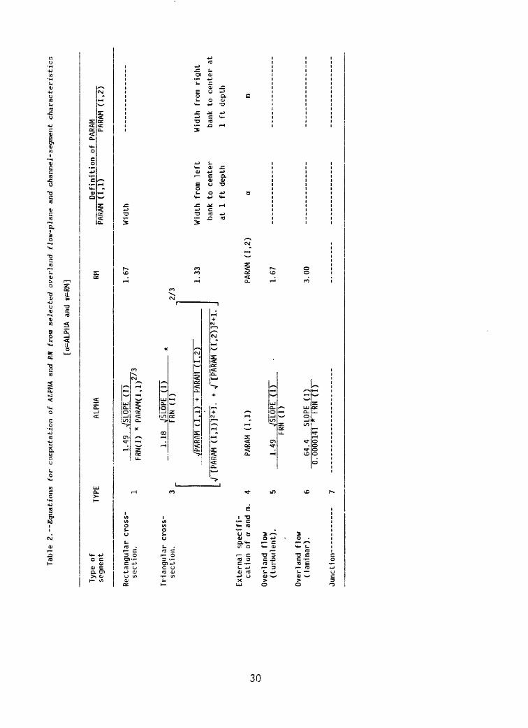
2. Equations for computation of ALPHA and RM from selectedoverland flow-plane and channel-segment characteristics 30
3. Model parameters and the associated values of the array,Lop 47
4. Major variables used in sensitivity-analysis components 605. List of subroutines included in cataloged procedure
PRMODEL 646. Data files developed in subroutine INVIN for stormflow-
hydrograph computations 677. List of input/output units and file structures 728. Default values for parameters specified on EXEC card 769. Input data-card groups needed for various model
configurations 7610. Parameter codes and statistic codes used for input data
types (IDUS) 83 11. List of channel segments delineated in figure 19b and
their upstream and lateral inflows 98

INTENTS--Continued
12. Variable identifiers used in output summary tables for basin averages and totals, and their definitions
13. Variable identifiers used in output summary tables forHRU values, and their definitions -
IV-1. Definitions of system variables -VI-1. System labeled common areas
Page
112
114182199
CONVERSION FACTORS
For use of readers who prefer to use metric units, conversion factors for terms used in this report are listed below.
Multiply
acreacre-inch (ac-in)calorie (cal)degree Fahrenheit (°F)foot (ft)foot per second (ft/s)square foot (ft 2 )cubic foot per second (ft 3/s)inch (in.)inch per day (in./d)inch per hour (in./hr)kilogram per square foot perper second (kg/ft 2 /s)
kilogram per cubic foot(kg/ft3 )
kilogram per cubic footper second (kg/ft 3 /s)
langley (ly)
'C=
By
0.4047 102.744.186
5/9 (°F-32)0.30480.30480.092940.028322.542.542.54
10.7635.31
35.314.186
To obtain
hectarecubic metersjouledegree Celsiusmetermeter per secondsquare metercubic meter per secondcentimetercentimeter per daycentimeter per hourkilogram per square meterper second
kilogram per cubic meter
kilogram per cubic meterper second
joule per square centimeter
National Geodetic Vertical Datum of 1929 (NGVD of 1929) A geodetic datum derived from a general adjustment of the first-order level nets of both the United States and Canada, formerly called mean sea level. NGVD of 1929 is referred to as sea level in this report.
vn

PRECIPITATION-RUNOFF MODELING SYSTEM: USER'S MANUAL
By G. H. Leavesley, R. W. Lichty, B. M. Troutman, and L. G. Saindon
ABSTRACT
The concepts, structure, theoretical development, and data requirements of the precipitation-runoff modeling system (PRMS) are described. The pre cipitation-runoff modeling system is a modular-design, deterministic, dis- tributed-parameter modeling system developed to evaluate the impacts of various combinations of precipitation, climate, and land use on streamflow, sediment yields, and general basin hydrology. Basin response to normal and extreme rainfall and snowmelt can be simulated to evaluate changes in water- balance relationships, flow regimes, flood peaks and volumes, soil-water relationships, sediment yields, and ground-water recharge. Parameter-optimi zation and sensitivity analysis capabilities are provided to fit selected model parameters and evaluate their individual and joint effects on model output. The modular design provides a flexible framework for continued model-system enhancement and hydro!ogic-modeling research and development.
INTRODUCTION
The precipitation-runoff modeling system (PRMS) is a modular-design modeling system that has been developed to evaluate the impacts of various combinations of precipitation, climate, and land use on surface-water runoff, sediment yields, and general basin hydrology. Basin response to normal and extreme rainfall and snowmelt can be simulated on various combinations of land use to evaluate changes in water-balance relationships, flow regimes, flood peaks and volumes, soil-water relationships, sediment yields, and ground-water recharge. PRMS is a deterministic physical-process modeling system. To reproduce the physical reality of the hydro!ogic system as closely as possi ble, each component of the hydro!ogic cycle is expressed in the form of known physical laws or empirical relationships that have some physical interpreta tion based on measurable watershed characteristics.
The modular design of PRMS provides a flexible modeling capability. Each component of the hydrologic system is defined by one or more subroutines that are maintained in a computer-system library. All subroutines are compatible for linkage to each other. Given a specific hydrologic problem and its associated data constraints, the user can select an established model from the library or can design his own model using selected library and user-supplied subroutines. The library also contains subroutines for parameter optimiza tion, sensitivity analysis, and model output handling and analysis. The initial system subroutines were obtained by modularizing an event-type dis tributed routing rainfall-runoff model (Dawdy and others, 1978) and a daily flow rainfall- and snowmelt-runoff model (Leavesley and Striffler, 1978), and by writing new algorithms for processes and procedures not available in these
models. Additional subroutines will be added and existing subroutines will be modified and improved as experience is gained from model applications in various climatic and physiographic regions.
PRMS is designed to function either as a lumped- or distributed-parameter type model and will simulate both mean daily flows and stormflow hydrographs. PRMS components are designed around the concept of partitioning a watershed into units on the basis of characteristics such as slope, aspect, vegetation type, soil type, and precipitation distribution. Each unit is considered homogeneous with respect to its hydrologic response and is called a hydrologic-response unit (HRU). A water balance and an energy balance are computed daily for each HRU. The sum of the responses of all HRU's, weighted on a unit-area basis, produces the daily system response and streamflow from the watershed. Partitioning provides the ability to impose land-use or climate changes on parts or all of a watershed, and to evaluate resulting hydrologic impacts on each HRU and on the total watershed.
Input variables include descriptive data on the physiography, vegetation, soils, and hydrologic characteristics of each HRU, and on the variation of climate over the watershed. The minimum driving variables required to run in the daily-flow mode are (1) daily precipitation, and (2) maximum and minimum daily air temperatures. Daily pan-evaporation data can be substituted for air temperature for situations where snowmelt simulation is not required; daily solar radiation data are recommended when snowmelt will be simulated. To simulate stormflow hydrographs, rainfall depths for time intervals of 60 minutes or less are required. PRMS is designed to run with data retrieved directly from the U.S. Geological Survey's National Water Data Storage and Retrieval (WATSTORE) system (Hutchinson, 1975). However, PRMS afso can use data not stored on the WATSTORE system. Programs are available to read and reformat these data to make them model-compatible.
The modular system approach provides an adaptable modeling system for both management and research applications. For management problems, a model can be tailored to geographic region, data, and problem characteristics. Research applications include development of new model components and the testing and comparison of various approaches to modeling selected components of the hydrologic cycle. New model components proposed as future additions to PRMS include water-quality components and expanded saturated-unsaturated flow and ground-water flow components.
This documentation is designed to provide the user with the basic philos ophy and structure of PRMS, instructions for application of established models designed as cataloged procedures, and instructions for interaction with the PRMS library to permit user additions or modifications of model compo nents. The components and subroutines described in this document are those available at the time of publication. However, the library is dynamic and will be enhanced and updated through time. This manual will be updated to reflect major additions and changes through manual inserts or republications.
All components of PRMS except the hydrologic and meteorologic data retrieval subroutines (DVRETR and UVRET) are written in FORTRAN. PRMS data sets are handled using an indexed sequential (ISAM) file structure. Because PRMS has been developed on an AMDAHL computer system, DVRETR and UVRET are

written in PL/I programming language. To run PRMS on computer systems that don't have ISAM file or PL/I-FORTRAN interface capabilities will require modifications to DVRETR and UVRET. Descriptions of DVRETR and UVRET are given in attachment VII to facilitate user modifications. Future enhancement of the data management components includes the development of a FQRTRAN-based data-management system. This system will permit creation, editing, and limited analysis of a PRMS data set.
SYSTEM STRUCTURE
The PRMS structure has three major components. The first is the data- management component. It handles the manipulation and storage of hydrologic and meteorologic data into a model-compatible direct access file. The second is the PRMS library component. This component consists of both a source- module library and a load-module library for the storage of the compatible subroutines used to define and simulate the physical processes of the hydro- logic cycle. In addition, it contains the parameter-optimization and sensitivity-analysis subroutines for model fitting and analysis. The third component is the output component that provides the model output handling and analysis capabilities.
The three PRMS components are shown schematically in figure 1. Hydro- logic and meteorologic field data are collected and stored in either user data files or the U.S. Geological Survey's WATSTORE system. Data interface pro grams accept data from these two sources and convert and store the data in an index-sequential (ISAM) file, which is fully model-compatible. The precipitation-runoff model either is selected as a cataloged procedure from the PRMS library or is created from PRMS library- and user-supplied subrou tines. The model reads initialization and basin characteristics information from card-deck input and accesses the ISAM data file for hydrologic and meteorologic data required for model operation. Model outputs can be printed and stored for further analysis.
The major components of the PRMS structure are discussed in greater detail in the following sections. Examples of the use of these components are given in attachments II and III.
Data Management
The U.S. Geological Survey WATSTORE system is used for permanent storage of hydrologic and meteorologic data. Field measurements are transmitted to the U.S. Geological Survey Computer Center in Reston, Va., where WATSTORE data reduction and input programs are used to store the data in the "Daily Values" and "Unit Values" files. Data in these files are identified by a unique station number and 5-digit parameter and statistic codes. STORET EPA parame ter codes are used to identify the type of data, and the statistic code defines the frequency of measurement or statistical reduction of the data. Lists and explanations of these codes may be found in Appendices D and E, Volume 1 of the WATSTORE user's manual (Hutchinson, 1975). Typically, the daily file will contain, for each day in the period of record, the maximum, minimum, and mean air temperature in degrees Celsius (°C), total solar radia tion in langleys per day (ly/d), total precipitation in inches, and mean

Mo
de
l-
Co
mp
atib
le
Dat
a
1.
Ra
infa
ll
2.
Snow
meit
3.
Se
dim
en
t
4.
...
Op
tion
2 u
ser
Se
lect
ed
Initia
lization
and
Bas
inC
hara
cterist
ics
Da
ta
Pre
cipi
tatio
n
Run
off
Mod
el
Out
put
Op
tion
s
Sta
tistical
an
aly
sis
Gra
ph
ics
inp
ut
to o
the
r m
odels
(L
ibra
ry o
r use
r su
pp
lied
)
Figu
re 1.
The
pre
cipi
tati
on-r
unof
f mo
deli
ng system.

discharge in cubic feet per second (ftVs). The unit file is used for storage of data collected at shorter time intervals, such as 5-minute precipitation and discharge. The WATSTORE system also has statistical, plot, and update capabilities that allow users to inspect and edit data.
The data-handling subroutines within the model do not access data direct ly from the WATSTORE system. The data-set organization required for use in the model is an indexed sequential (ISAM) file containing both daily- and unit-values data. A cataloged procedure, GENDISK, is available to read sequential files containing standard WATSTORE daily- and unit-values records and create the model-compatible ISAM file. Data contained in the WATSTORE system are made available to GENDISK by executing standard daily- and unit- values retrieval programs. The ISAM file may contain more data than are needed for any particular model run, since the data-handling subroutines within the model will automatically select the years and events requested on the model control cards. However, if more data than are initially included in the ISAM file are required, the file must be recreated, since additions cannot be made to it.
System Library
The system library is the core of the PRMS. It contains all the compati ble subroutines that can be used in system-defined or user-defined combina tions to simulate the hydrologic cycle. The structure of the library and its subroutines is based on two model-design concepts. The first is that a MAIN program will be used as a central point for time and computational sequence control. Timing control maintains day, month, and year variables and incre ments them as required. Sequence control establishes the framework in which the sequence of various model functions will be performed. These functions are performed by calls to appropriate library subroutines. The timing and sequence functions are discussed in more detail in subsequent sections. The second concept is that each subroutine represents one component of the hydro- logic cycle and is designed to be as independent as possible from other component subroutines. The necessary transfer of information between subrou tines is done using COMMON statements.
The PRMS library is composed of both a source-module library and a load- module library. The source-module library contains the FORTRAN coded subrou tines. The load-module library consists of the compiled subroutines ready for linkage editing into a complete program. Instructions for obtaining a copy of the source-module library are given in attachment V.
The library provides the user several options in model development and application. One option is the use of the cataloged procedure PRMODEL, which is the compilation of the complete model system. A second option would be to compile a new model using the System MAIN program with a combination of library- and user-supplied subroutines. A third option would be for the user to write his own MAIN program and use a combination of library- and user-supplied subroutines. This manual primarily is directed to the first option. However, the last two options are discussed in detail in the System Modification section.

Output
The output component provides the user with several options for analyz ing, displaying, and storing model simulation results. Options include various printed summaries, printer plots of observed and predicted streamflow and sediment, and storage of observed and predicted streamflow for use with PRMS library, WATSTORE, Statistical Analysis System (SAS) (SAS Institute Inc., 1982), or user-written analysis programs. Desired outputs are specified in the data input stream.
Printed output options range from a table of predicted and -observed streamflow values to annual, monthly, daily, or storm-event streamflow summa ries. Annual, monthly, or daily summaries also are available for major climate and water-balance elements. These detailed summaries are available both for the total basin and for each individual HRU.
Predicted mean daily streamflow data can be stored by water year as a permanent file for further processing and analysis. Two record formats are available for data storage. One is the standard WATSTORE daily-value format, which permits the use of WATSTORE and SAS analysis programs. The second format option is designed for PRMS library and user-written analysis programs. It contains only the water-year date and 366 data values.
The output component is discussed in more detail in the System Output section. Examples of the output options are shown in the System Output section and in the sample model runs in attachment II.
SYSTEM CONCEPTS
The objectives established to guide the design and development of PRMS were that PRMS should:
1. Simulate mean daily flows and shorter time-interval stormflowhydrographs for any combination of precipitation, climate, and land use.
2. Provide model-modification capabilities to permit specific user requirements or limitations to be incorporated.
3. Provide capabilities for system enhancement and expansion.4. Provide error and sensitivity-analysis capabilities.5. Provide a data-management capability that is compatible with the
U.S. Geological Survey WATSTORE system, but adaptable to other computer systems.
A modular system design was selected to provide the desired flexibility and data-management capabilities, and to allow incorporation of user-specific requirements.
The major component of PRMS is the system library. The use of models or components from the library requires an understanding of the basic concepts used in its design and development. These include the conceptual model of the watershed system, the partitioning scheme used to provide distributed- parameter modeling capabilities, the time basis of model operation, and the interface between daily flow and stormflow hydrograph-generation components.

Conceptual Watershed System
The watershed system and its inputs are schematically depicted in figure 2. System inputs are precipitation, air temperature, and solar radia- ion. Precipitation in the form of rain, snow, or a mixture of both is reduced by interception and becomes net precipitation delivered to the watershed surface. The energy inputs of temperature and solar radiation drive the pro- esses of evaporation, transpiration, sublimation, and snowmelt. The watershed system is conceptualized as a series of reservoirs whose outputs combine to produce the total system response.
The impervious-zone reservoir represents an area with no infiltration capacity. The reservoir has a maximum retention storage capacity (RETIP) which must be satisfied before surface runoff (SAS) will occur. Retention storage is depleted by evaporation when the area is snow free.
The soil-zone reservoir represents that part of the soil mantle that can lose water through the processes of evaporation and transpiration. Average rooting depth of the predominant vegetation covering the soil surface defines the depth of this zone. Water storage in the soil zone is increased by infiltration of rainfall and snowmelt and depleted by evapotranspiration. Maximum retention storage occurs at field capacity; minimum storage (assumed to be zero) occurs at wilting point. The soil zone is treated as a two- layered system. The upper layer is termed the recharge zone and is user- defined as to depth and water-storage characteristics. Losses from the recharge zone are assumed to occur from evaporation and transpiration; losses from the lower zone occur only through transpiration.
The computation of infiltration into the soil zone is dependent on whether the input source is rain or snowmelt. All snowmelt is assumed to infiltrate until field capacity is reached. At field capacity, any additional snowmelt is apportioned between infiltration and surface runoff. At field capacity the soil zone is assumed to have a maximum daily snowmelt infiltra tion capacity, SRX. All snowmelt in excess of SRX contributes to surface runoff. Infiltration in excess of field capacity (EXCS) first is used to satisfy recharge to the ground-water reservoir (SEP). SEP is assumed to have a maximum daily limit. Excess infiltration, available after SEP is satisfied, becomes recharge to the subsurface reservoir. Water available for infiltra tion as the result of a rain-on-snow event is treated as snowmelt if the snowpack is not depleted, and as rainfall if the snowpack is depleted.
For rainfall with no snowcover, the volume infiltrating the soil zone is computed as a function of soil characteristics, antecedent soil-moisture conditions, and storm size. For daily-flow computations, the volume of rain that becomes surface runoff is computed using a contributing-area concept. Daily infiltration is computed as net precipitation less surface runoff . For stormflow-hydrograph generation, infiltration is computed using a form of the Green and Ampt equation (Philip, 1954). Surface runoff for these events is net precipitation less computed infiltration. Infiltration in excess of field capacity is treated the same as daily infiltration.

CO
Eva
potr
an
INP
UTS
sPjra
tion
te
mpe
ratu
re
Pre
cipita
tion
Jola
r^
iE
vapo
ratio
nS
ublim
atio
n
Sub
limat
ion
Eva
pora
tion
""""
C T
rans
pira
tion
_ _
Rld
llr*
4 _ . .
Low
erT
ran
sp
ira
tio
n
F
Inte
rce
ptio
n
Thro
u Jghfa
llt
>s
Sno
wpa
ck
,
......
f E
vaoo
ratio
n
Sno
w /je
zon
e
zone
ne
lt t
V ,-
1 S
urfa
ce r
unof
f (S
AS
)Im
perv
ious
zon
e re
serv
oir
Sur
face
run
off
(SA
S)
) *
\ S
oil
zone
j
rese
rvo
ir
TS
oil
zone
ex
cess
(E
XC
S)
/S
ubsu
rfac
e re
char
ge (
EX
CS
-SE
P)
/
Subs
re
ssurf
ace
erv
oir
Sub
surf
ace
flow
(R
AS
)G
rou
nd
- wat
er
f ...-.._
_. -,
re
char
ge (
SEP)
G
roun
d -w
ate
r I
rech
arge
(G
AD
) 1
4G
roun
d -w
ate
r re
serv
oir
Gro
und
-wate
r flo
w (
BA
S)
'S
trea
mflo
wI
Gro
un
d-w
ate
r si
nk
(SN
K)
I
Figu
re 2
.--S
chem
atic
diagram o
f th
e co
ncep
tual
wa
ters
hed
syst
emand
its
inpu
ts.

The subsurface reservoir performs the routing of soil-water excess that percolates to shallow ground-water zones near stream channels or that moves downslope from point of infiltration to some point of discharge above the water table. Subsurface flow (RAS) is considered to be water in the saturated-unsaturated and ground-water zones that is available for relatively rapid movement to a channel system. The subsurface reservoir can be defined either as linear or nonlinear.
Recharge to the ground-water reservoir can occur from the soil zone (SEP) and the subsurface reservoir (GAD). SEP has a daily upper limit and occurs only when field capacity is exceeded in the soil zone. GAD is computed daily as a function of a recharge rate coefficient (RSEP) and the volume of water stored in the subsurface reservoir. The ground-water reservoir is a linear reservoir and is the source of all baseflow (BAS). Movement of water through the ground-water system to points beyond the area of interest or measurement can be handled by flow to a ground-water sink (GSNK) which is computed as a function of storage in the ground-water reservoir.
Streamflow is the sum of SAS, RAS, and BAS. For daily flow simulations, no channel routing is done.
Watershed Partitioning
The distributed-parameter modeling capability is provided by partitioning a watershed into "homogeneous" units. Watershed partitioning can be done on the basis of characteristics such as slope, aspect, elevation, vegetation type, soil type, and precipitation distribution. Each watershed unit delin eated is considered to be homogeneous with respect to these characteristics. Partitioning provides the ability to account for spatial and temporal varia tions of basin physical and hydrologic characteristics, climatic variables, and system response. It also provides the ability to impose land-use or climatic changes on parts or all of a basin. Evaluation can then be made cf the impacts of such changes on the hydrology of each unit and the total basin.
Two levels of partitioning are available. The first level divides the basin on the basis of some or all of the physical characteristics mentioned above. The resulting units are called hydrologic response units (HRU's), and each is considered homogeneous with respect to its hydrologic response. A water balance and an energy balance are computed daily for each HRU. The sum of the responses of all HRU's, weighted on a unit-area basis, produces the daily system response and streamflow from a basin.
The conceptual watershed system shown in figure 2 could be defined for each HRU. However, for most small watersheds, one soil-zone reservoir is defined for each HRU, while one ground-water reservoir is defined for the entire watershed. One or more subsurface reservoirs are defined, depending on variations in soils and geology.
PRMS will handle a maximum of 50 HRU's. The number and location of HRU's for any given basin are a function of the number of physical characteristics used in the partitioning scheme, the number and location of precipitation

gages available, and the problem to be addressed by the model. There are no hard and fast rules for partitioning currently available; this is an area to be addressed by further research. However, the number of HRU's delineated will influence the calibration fit of many of the model components (Leavesley and Striffler, 1978). A general rule of thumb currently used, for daily-flow computations for most problems is not to create HRU's smaller than 4 to 5 percent of the total basin area. Exception would occur if an area smaller than this would have significant influence on streamflow or on general basin hydrology. A common tendency is to overpartition. Therefore, it is recom mended that test runs be made at a few levels of partitioning to get a feel for the influence of the numbers of HRU's on model daily-flow response.
A second level of partitioning is available for storm hydrograph simula tion. The watershed can be conceptualized as a series of interconnected flow-planes and channel segments. Surface runoff is routed over the flow planes into the channel segments; channel flow is routed through the watershed channel system. An HRU can be considered the equivalent of a flow plane, or it can be delineated into a number of flow planes. Delineation of a basin into 6 overland flow planes and 3 channel segments is shown in figure 3. Overland flow planes have a width equal to the adjacent channel segment, and an equivalent length which, when multiplied by the width, gives the area of the natural basin segment. PRMS will handle a total of 50 overland flow plane and 50 channel segments.
Daily and Storm Modes
A model selected or developed from the PRMS library can simulate basin hydrology on both a daily and a storm time scale. The daily mode simulates hydro!ogic components as daily average or total values. Streamflow is comput ed as a mean daily flow. The storm mode simulates selected hydrologic compo nents at time intervals shorter than a day. The minimum time interval is 1 minute. The storm mode is used to compute infiltration, surface-water runoff, and sediment yield from selected rainfall events.
Data required for daily simulations are input to the model 1 water year at a time. Included in the input are the dates of storm periods within the water year, where data are available for rainfall-runoff simulations. The model operates in a daily mode until it reaches one of these dates. It then shifts to the storm mode and inputs the data available for that date. A stormflow hydrograph and sediment-concentration graph can be simulated for that day at a time interval selected by the user. At the end of the storm day, control is returned to selected daily components for updating to insure storm- and daily-mode compatibility and to compute mean daily streamflow. If the storm period is more than 1 day in length, then control returns to the storm mode and another day of data is input. Subsequent storm days of data are read and used in this manner until the storm period terminates. The model then returns to the full daily-mode sequence.
Summaries can be output both for daily and for storm simulations. Daily mode computations can be summarized on a daily, monthly, and annual basis. Storm-mode computations can be summarized for the full storm period and at a user-selected time interval.
10

HYDROLOGIC-RESPONSE UNIT DELINEATION
EXPLANATION
3 ) Channel segment and number
Flow-plane and number
Figure 3. Flow-plane and channel-segment delineation of a basin.
11

The daily mode keeps account of days using a day-month-year scheme and three numerical sequencing indices that number days of the year from 1 to 365 or 366. One numerical index is the Julian date. This numbers the days of the year beginning on January 1. A water-year date index also is used; it begins day 1 on October 1. The third numerical index is the solar date. Day 1 begins on December 22, which is the winter solstice, or the date of receipt of minimum potential solar radiation.
THEORETICAL DEVELOPMENT OF SYSTEM LIBRARY COMPONENTS
Meteorologic Data
The meteorologic data components take temperature and solar radiation data from one station and precipitation data from up to 5 gages and adjust these data for each HRU. Adjustment factors are computed as functions of the differences in elevation, slope, and aspect between the measuring station and each HRU. Local and regional climate and precipitation data are the sources for the development of these adjustment factors.
Temperature
Observed daily maximum (TMX) and minimum (TMN) air temperatures are adjusted to account for differences in elevation and slope-aspect between the climate station and each HRU. Air-temperature data can be input either in Fahrenheit (°F) or in Celsius (°C), but these data must be consistent through out a simulation. All temperature variables and parameters must be in the same units as the temperature data. All daily maximum, minimum, and mean air-temperature computations are made in subroutine TEMP.
A correction factor (TCRX) for adjusting TMX for each HRU is computed each month (MO) by:
TCRX(MO) = [TLX(MO) * ELCR] - TXAJ (1)
where
TLX is the maximum temperature lapse rate, in degrees per 1,000 feetchange in elevation for month MO;
ELCR is the mean elevation of an HRU minus the elevation of the climatestation, in 1,000's of feet; and
TXAJ is an average difference in maximum air temperature between ahorizontal surface and the slope-aspect of an HRU.
A correction factor [TCRN(MO)] for adjusting TMN for each HRU is computed monthly with an equation of the same form as equation 1, using the monthly minimum temperature lapse rate [TLN(MO)] and minimum temperature slope-aspect correction (TNAJ).
Adjusted daily maximum air temperature (TM) for each HRU is computed by:
TM = TMX - TCRX(MO) (2)
12

Adjusted daily minimum air temperature (TN) for each HRU is computed using an equation of the same form as equation 2 and the variables TMN and TCRN(MO).
Precipitation
Total daily precipitation depth (PPT) received on an HRU is computed by:
PPT = PDV * PCOR (3)
where
PDV is the daily precipitation depth observed in the precipitationgage associated with the HRU, in inches (in.), and
PCOR is the correction factor for the HRU.
A maximum of five gages can be used to define the spatial and temporal varia tion of precipitation on a watershed. Each HRU is associated with one of the available gages by the precipitation gage index KDS. A PCOR value is defined for each HRU and relates to the gage specified by KDS. PCOR accounts for the influences of elevation, spatial variation, topography, and gage-catch effi ciency. Different values of PCOR can be specified for different precipitation forms and time scales of measurement--DRCOR for daily rainfall, DSCOR for daily snowfall, and UPCOR for storm-mode rainfall. In some geographic and climatic regions, the influence of elevation on precipitation volume varies seasonally with general storm patterns (Barry, 1972). Frontal origin storms may show a strong elevation effect, while convective storms may show little elevation effect. If DRCOR and DSCOR include strong elevational influence, they can be overridden for a period of time to account for these seasonal changes. All HRU values of DRCOR are replaced by a single constant value PCONR and all values of DSCOR are replaced by a constant value PCONS. The override period is user-specified to begin on the first day of month MPCS and end on the first day of month MPCN.
Precipitation form (rain, snow, or mixture of both) on each HRU is estimated from the HRU maximum (TM) and minimum (TN) daily air temperatures and their relationship to a base temperature (BST) (Will en and others, 1971). Precipitation is all snow if TM is less than or equal to BST, and all rain if TN is greater than BST. If TM is greater than BST and TN is less than BST, then the part of the total precipitation occurring as rain (PRMX) is computed
where
PRMX = * AJMX(MO) (4)
AJMX is a monthly mixture adjustment coefficient for month MO. For mixed events, rain is assumed to occur first.
13

The mixture algorithm can be overridden in two ways. One is the use of variable PAT. PAT is an air- temperature value which, when exceeded by TM, forces all precipitation to be rain, regardless of the TN value. This capa bility permits accounting for convective rainfall during spring, when minimum daily temperatures are below BST. PAT is user-specified for each month. The second override is used when the form of precipitation is known by the user. Precipitation form then can be specified, using the snow and rain data cards (Card Group 5). These cards designate the Julian dates in each water year that are to be considered all snow or all rain.
All of the computations described above are made in subroutine PRECIP. One additional subroutine, PKADJ, is available for adjusting precipitation input. For snow, gage-catch deficiencies of about 45 to 70 percent can be expected at wind speeds of 10 to 20 miles per hour (Larson and Peck, 1974). To account for gage-catch deficiencies, PKADJ provides the capability of adjusting the snowpack water equivalent on each HRU, based on snowcourse data from each HRU or an index snowcourse. This adjustment option is available only once each year; therefore, it is best used near the anticipated date of maximum snowpack accumulation.
Solar Radiation
Observed daily shortwave radiation (ORAD) expressed in langleys per day (ly/d) is used in snowmelt computations and can be used in evapotranspi ration computations. ORAD is an optional input for areas with no snowmelt. For areas where snowmelt will be simulated, ORAD can be input directly or estimat ed from daily air- temperature data for watersheds where it is not available. All solar radiation computations are made in subroutines SOLRAD and SOLTAB.
ORAD, measured on a horizontal surface, is adjusted to estimate SWRD, the daily shortwave radiation received on the slope-aspect combination of each HRU. SWRD is computed by:
SWRD = ORAD * (5)
whereDRAD is the daily potential solar radiation for tha slope and aspect
of an HRU (ly), and HORAD is the daily potential solar radiation for a horizontal
surface (ly).
DRAD and HORAD are linearly interpolated from a table of 13 potential solar radiation values (RAD), which are calculated for each slope-aspect combination and the horizontal surface. Because of the symmetry of the solar year, these 13 values represent potential solar radiation for 24 dates throughout the year. The 13 dates and date pairs are listed in table 1. Table values are computed in subroutine SOLTAB using a combination of methods described in Frank and Lee (1966) and Swift (1976).
14

Table 1. Sequence number and dates of the 13 potential solar radiation values for each slope-aspect combination
SequenceNo. Date(s)
1 December 222 January 10, December 33 January 23, November 194 February 7, November 55 February 20, October 22 5 March 7, October 8 7 March 21, September 23 Q April 4, September 9 9 April 19, August 25
IQ May 3> August 10 n May 18) July 2712 june i } j uly 1213 June 22
For missing days or periods of record, ORAD can be estimated from air- temperature data. One of two procedures can be selected using variable MRDC. The first is a modification of the degree-day method described by Leaf and Brink (1973). This method was developed for a section of the Rocky Mountain Region of the United States. It appears most applicable to this region of the country, where predominantly clear skies prevail on days without precipitation.
The method is shown graphically in the coaxial relation of figure 4. A daily maximum temperature is entered in the X-axis of part A and intersects the appropriate month curve. From this intersection point, one moves horizon tally across the degree-day coefficient axis and intersects the curve in part B. From this point, the ratio of actual-to-potential radiation for a horizon tal surface (SOLF) can be obtained. An estimate of ORAD is then computed by:
ORAD = SOLF * HORAD. (6)
The ratio SOLF is developed for days without precipitation; thus, the computed ORAD is for dry days. ORAD for days with precipitation is estimated for the period September through April by multiplying the ORAD from equation 6 by a user-defined constant PARW. For days with precipitation in the months May through August, ORAD is adjusted using PARS in place of PARW.
The input data required to use this procedure are the slope (RDM) and the y-intercept (RDC) of the line that expresses the relationship between monthly maximum air temperature and a degree-day coefficient (DD). Estimates
15

DE
GR
EE
-DA
Y C
OE
FFIC
IEN
T (D
D)
CT1
CQ
C -5 (D
-5
£>
O)
C
L
I_j.
|PJ
m
r+
X_.
. O)
O
3
13
T
J __i
-t> r
o-5
O
O
3
OCU
O
X
0)3
-
X
O
3-3
C
c+
3
DJ
O.
-5CD
in
rt>
en
_i. i
3
0)
O-
' r3
O
~5
«/>o
rr
-j <
+ -
o
ro -
a-5
3
Cu
TJ
-ha.
ro
o0-5
-5
- a»
c+
tt>
c
</>-S
r+
ro
-
ro
3 '(
Q
O
TJ
Ul
rt>
r?-
Q.
O
"5-h
r+
o s:
O)
oo_
Jh
*
*
-A
*
KJ
O
M
J»
CD
00
O
O t>
-*
2
o
>
X 35
§
3 g 3D m 2
-n m
og
>5
56
</>
oQ
""
"I ?l O
P 13
S3
Ǥ
Q
i _»S 00 o 8
I I
I I
I I
I I
I I
I I
I I
I I
I 1
I I
! I
I i
I
>
H
i i
i i
i i
i i
i i
i i
i i
i
i i
i i
ii
i ii
IT
i il
l i
i i
rn ii
r
I I
I I J_
I i
I_
III_
I
I I
I I
I I
I I
I I
I I
I
of PARW and PARS also are required. DD is computed by:
DD = (RDM * TMX) + RDC (7)
where TMX is the observed daily maximum air temperature. The DD-SQLF rela tionship of figure 4 is assumed constant.
Monthly values of RDM and RDC can be estimated from historic air- temper ature and solar-radiation data. One method is to make monthly plots of TMX versus their daily degree-day coefficients, DD, for days without precipita tion. The DD values for this plot are computed using figure 4 and the daily SOLF ratios computed from historic data. A set of monthly lines then can be drawn through these points either visually or with linear- regression tech niques. A more rapid and coarse procedure is to establish two points for each monthly line using some average values. One point for each month is estimated using the average SOLF and average maximum temperature for days without precipitation. The second point is estimated using the maximum observed temperature for each month and a DD value of 15. Using this second procedure, curves shown in part A of figure 4 were estimated for a region in northwest Colorado. Estimates of PARW and PARS are obtained from the radiation record. PARW is the ratio of SOLF for days with precipitation to days without precipi tation over the September through April period. PARS is the ratio of SOLF for days with precipitation to days without precipitation over the May through August period.
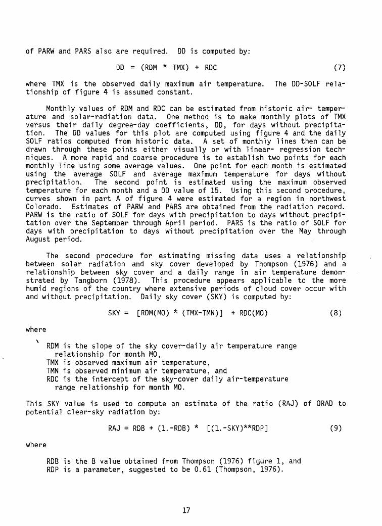
The second procedure for estimating missing data uses a relationship between solar radiation and sky cover developed by Thompson (1976) and a relationship between sky cover and a daily range in air temperature demon strated by Tangborn (1978). This procedure appears applicable to the more humid regions of the country where extensive periods of cloud cover occur with and without precipitation. Daily sky cover (SKY) is computed by:
SKY = [RDM(MO) * (TMX-TMN)] + RDC(MO) (8)
where
RDM is the slope of the sky cover-daily air temperature rangerelationship for month MO,
TMX is observed maximum air temperature, TMN is observed minimum air temperature, and RDC is the intercept of the sky-cover daily air-temperature
range relationship for month MO.
This SKY value is used to compute an estimate of the ratio (RAJ) of ORAD to potential clear-sky radiation by:
RAJ = RDB + (l.-RDB) * [(l.-SKY)**RDP] (9)
where
RDB is the B value obtained from Thompson (1976) figure 1, and RDP is a parameter, suggested to be 0.61 (Thompson, 1976).
17

For days with precipitation, RAJ is multiplied by PARS (May through August) or PARW (September through April). An upper limit on RAJ is specified by the parameter RDMX. ORAD is then computed by:
ORAD = RAJ * HORAD (10)
Both ORAD estimation procedures are relatively coarse, but appear to work reasonably well. They normally are used to fill in days of missing data. However, where radiation data are unavailable, they have produced reasonable results when used to generate entire periods of solar-radiation record. In such cases, the nearest climate station with radiation and air-temperature data is used to estimate RDM and RDC values. If there is a large difference in elevation between the climate station on the watershed and the station with radiation data, the air-temperature data associated with the radiation data are adjusted to the study-basin elevation.
Impervious Area
Impervious area can be treated in one of two ways. If it exists as large, contiguous areas, then it can be designated as one or several totally impervious HRU's. If it is of significant area but scattered throughout the pervious areas of a watershed, then impervious area can be expressed as composing a percentage of an otherwise pervious HRU. Interception is assumed not to occur on impervious areas. Therefore, input to impervious areas is total precipitation. Impervious surface is assigned a maximum retention storage capacity (RETIP). Available retention storage (RSTOR) is depleted by evaporation. Surface runoff from impervious areas is delivered directly to the channel network and occurs only after RETIP is filled.
Interception
Interception of precipitation is computed as a function of the cover density and the storage available for the predominant vegetation on an HRU. Net precipitation (PTN) is computed by:
PTN = [PPT * (l.-COVDN)] + (PTF * COVDN) (11)
where
PPT is the total precipitation received on an HRU (in.),COVDN is the seasonal cover density, andPTF is the precipitation falling through the canopy (in.).
COVDN is defined for summer (COVDNS) and winter (COVDNW). PTF is computed by:
PTF = PPT - (STOR-XIN) PPT > (STOR - XIN) (12) PTF =0.0 PPT < (STOR - XIN)
whereSTOR is the maximum interception storage depth
on vegetation (in.), and XIN is the current depth of interception storage (in.).
18

STOR is defined by season and precipitation form winter snow (SNST), winter rain (RNSTW), and summer rain (RNSTS). When rain falls on intercepted snow, STOR changes from SNST to the seasonal rain-storage value. Any snow in storage that exceeds the new rain-storage value is added to throughfall PTF. When snow falls on intercepted rain, STOR changes to SNST and currently available rain interception is used to satisfy SNST. Intercepted rain in excess of SNST is added to PTF. SNST generally is considered to be greater than or equal to RNSTW. PTF and XIN are computed in subroutine PRECIP for daily-precipitation events, and in subroutine UNITD for storm events.
Intercepted rain is assumed to evaporate at a free-water surface rate (EVCAN). If pan-evaporation data are used, then EVCAN equals the pan loss. If potential evapotranspi ration (PET) is computed from meteorologic variables, EVCAN is computed by:
EVCAN =
where EVC is the evaporation-pan coefficient for month MO. Sublimation of intercepted snow (SUBCAN) is assumed to occur at a rate that is expressed as a percentage (CTW) of PET. In addition to sublimation, intercepted snow can be removed from the canopy by melting. An energy balance is computed for a 12-hour period (assumed 0600 to 1800). If the energy balance is zero or negative, no melt occurs. When the energy balance is positive, all melt is delivered to the snowpack or soil surface as net precipitation.
Actual daily loss from interception (XINLOS) is equal to the smaller value of storage XIN or loss rates, EVCAN or SUBCAN. If XIN is not depleted in I day, the remainder is carried over to the next day. XINLOS, as computed above, represents loss from the percentage of HRU area expressed in the cover density parameters COVDNS or COVDNW. For water balance computations, XINLOS is adjusted to represent an HRU average value. XINLOS is computed in subrou tine INTLOS in the daily mode and in subroutine UNITD in the storm mode.
Soil -Moisture Accounting
Soil -moisture accounting is performed as the algebraic summation of all moisture accretions to, and depletions from, the active soil profile. Deple tions include evapotranspi ration and recharge to the subsurface and ground- water reservoirs. Accretions are rainfall and snowmelt infiltration. The depth of the active soil profile is considered to be the average rooting depth of the predominant vegetation on an HRU. The maximum available water-holding capacity of the soil zone (SMAX) is the difference between field capacity and wilting point of the profile. The active soil profile is divided into two layers. The upper layer is termed the recharge zone and the lower layer is termed the lower zone. The recharge zone is user-definable as to depth and maximum available water-holding capacity (REMX). The maximum available water-holding capacity (LZMX) of the lower zone is the difference between SMAX and REMX. Losses from the recharge zone occur from evaporation and
19

transpiration; they occur only as transpiration from the lower zone. Evapotranspiration losses occur at a rate that is a function of available soil-moisture storage. The attempt to satisfy potential evapotranspiration is made first from the recharge zone. Soil-moisture accretions must fill the recharge zone storage before water will move to the lower zone. When soil-zone storage reaches SMAX, all additional infiltration is routed to the subsurface and ground-water reservoirs.
Soil-moisture accounting for daily computations is done in subroutine SMBAL. Accounting computations for storm-event periods are done in subroutine UNITD.
Evapotranspi rati on
Daily estimates of potential evapotranspiration (PET) are computed in subroutine PETS. Three computation procedures are available. Procedure selection is made, using variable IPET. The first procedure uses daily pan-evaporation data. PET (in./day) is computed by:
PET = EPAN * EVC(MO) (14)
where
EPAN is daily pan-evaporation loss, (in.), andEVC is a monthly pan-adjustment coefficient for month MO.
A second procedure computes PET as a function of daily mean air tempera ture and possible hours of sunshine (Hamon, 1961). PET (in./d) is computed by:
PET = CTS(MO) * DYL2 * VDSAT (15)
where
CTS is a coefficient for month MO,DYL is possible hours of sunshine, in units of 12 hours, and VDSAT is the saturated water-vapor density (absolute humidity) at
the daily mean air temperature in grams per cubic meter (g/m3 ).
VDSAT is computed by (Federer and Lash, 1978):
SAT = 216 ' 7 * (TAvTf273.3) (16)
where
VPSAT is the saturated vapor pressure in millibars (mb) at TAVC, and TAVC is the daily mean air temperature (°C).
20

VPSAT is computed by (Murray, 1967):TAVP
VPSAT = 6.108 * EXP [17.26939 * (TAVC + 237 3) ] (17)
Hamon (1961) suggests a constant value of 0.0055 for CIS. Other investigators (Leaf and Brink, 1973; Federer and Lash, 1978) have noted that 0.0055 underes timated PET for some regions. Limited experience also has shown that a constant annual value underestimates PET for winter months more than summer months. Therefore, the ability to vary CTS by month is provided. DYL will vary with time of year and HRU slope and aspect. A set of day-length values (SSH) in hours is computed in subroutine SOLTA8 for 13 specified date-pairs throughout the year (table 1) for each solar-radiation plane. Each SSH value is divided by 12 to compute its associated DYL value. Daily DYL values are interpolated from the 13 DYL values in subroutine SOLRAD.
The third procedure is one developed by Jensen and Haise (1963). PET (in./d) is "computed by:
PET = CTS(MO) * (TAVF-CTX) * RIN (13)
where
CTS is a coefficient for the month MO, TAVF is the daily mean air temperature (°F), CTX is a coefficient, andRIN is daily solar radiation expressed in inches of evaporation
potential .
As with the Hamon procedure, the Jensen-Haise procedure also tends to underestimate winter month PET. Therefore, the ability to change CTS by month is provided. For the warmer months of the year, constant values for CTS and CTX can be estimated using regional air temperature, elevation, vapor pres sure, and vegetation data (Jensen and others, 1969). For aerodynamical ly rough crops, which are assumed to include forests, CTS is computed for the watershed by: -,
CTS = [Cl + (13.0 * CH)]"" 1 (19)
where
Cl is an elevation correction factor, and CH is a humidity index.
Cl is computed by:
Cl = 68.0 - [3.6 * ( )] (20)
where
El is the median elevation of the watershed (ft).
21

CH is computed by:CH = (iF^T)
where
e« is the saturation vapor pressure (mb) for the mean maximum air temperature for the warmest month of the year, and
e, is the saturation vapor pressure (mb) for the mean minimum air temperature for the warmest month of the year.
CTX is computed for each HRU by:F9
CTX = 27.5 - 0.25 * (e2 - ej - ( ^g^) (22)
where
E2 is the median elevation of the HRU (ft).
Actual evapotranspi ration (AET) is the computed rate of water loss which reflects the availability of water to satisfy PET. When available water is nonlimiting, AET equals PET. PET is first satisfied from interception stor age, retention storage on impervious areas, and evaporation/sublimation from snow surfaces. Remaining PET demand then is applied to the soil -zone storage. AET is computed separately for the recharge zone and the lower zone using the unsatisfied PET demand and the ratio of currently available water in the soil zone to its maximum available water-holding capacity. For the recharge zone*u- «.- RECHR _ _, , , SMAV . j A +. A this ratio is .,.. For the lower zone the ratio is used. AET computed~
for the recharge zone is used first to satisfy PET; any remaining demand is attempted to be met by AET from the lower zone. HRU soils are designated as being predominantly sand, loam, or clay, using variable ISOIL. The AET-PET relations for these soil types as a function of the soil -water ratio are shown in figure 5 (Zahner, 1967). AET computations are done in subroutine SMBAL.
The time of the year in which transpiration occurs is specified as a period of months between ITST and ITND, which are the starting (ITST) and ending (ITND) months of the transpiration period. The specific date of the start of transpiration is computed for each HRU^ using the temperature- index parameter TST. For each HRU, the sum of the daily maximum air temperatures is accumulated, starting with the first day of month ITST. When the sum for an HRU exceeds TST, transpiration is assumed to begin on that HRU. This tech nique permits accounting in part for warmer- or colder-than-normal spring periods. Transpiration is assumed to stop on the first day of ITND.
22

1.00
0.75
C 0.50OL
°'25
O.
12LU
0
1.00
0.75
Z 0.50
2Z 0.25O
O. CO
S 1.008UJ 0.75
D
q 0.50
0.25
Sand
Loam
Clay
0 0.25 0.50 0.75 1.00
CURRENT WATER AVAILABLE/MAXIMUM WATER STORAGE
(RECHR/REMX or SMAV/SMAX)
Figure 5. Soil-water withdrawal functions for evapotranspiration(modified from Zahner, 1967).
23

Infiltration
Infiltration computations vary depending on the time interval and the form of the precipitation input. For daily rainfall occurring on a snow-free HRU, infiltration is computed as the difference between net rainfall computed in subroutine PRECIP and surface runoff computed in subroutine SRFRO. For snowmelt, infiltration is assumed nonlimiting until the soil reaches field capacity. Once field capacity is reached, a user-defined daily maximum infiltration capacity (SRX) limits the daily-infiltration volume. Any snowmelt in excess of SRX becomes surface runoff. For rain-on-snow, the resulting water available for infiltration is treated as snowmelt if the snowpack is not depleted. If the snowpack is depleted, then the rain and snowmelt are treated as rain on a snow-free surface.
Storm-mode computations are made only for rainfall and only when the basin is snow free. Infiltration during storms is computed in subroutine UNITD, using a variation of the Green- Ampt equation (Green and Ampt, 1911). Net rainfall (PTN) reaching the soil surface is allocated to rainfall excess (QR) and infiltration (FIN), either at the user-specified time interval or at 5 minutes, whichever is less. Point- infiltration capacity (FR) is computed
FR = KSAT * (1.0 + -~) (23)
where
KSAT is hydraulic conductivity of the transmission zone ininches per hour,
PS is effective value of the product of capillary driveand moisture deficit (in.), and
SMS is the current value of accumulated infiltration (in.).
RECHRPS is varied linearly as a function of the ratio REMX over the range from PSP, the value of the product of capillary drive and moisture deficit at field capacity, to a maximum value, RGF times PSP, expressed as:
PS = PSP * [RGF - (RGF-I) * (ff§T)L (24)
where
RECHR is the current moisture storage in the recharge zone ofthe soil profile (in.), and
REMX is the maximum moisture storage in the recharge zoneof the soil profile (in.).
24

This relationship is shown in figure 6. Net infiltration FIN then is com puted, assuming that infiltration capacity varies linearly from zero to FR (fig. 7). Thus, FIN is computed as:
FIN = PTN - ~- PTN < FR (25)
FR FIN = otherwise.
Rainfall excess (QR) is simply the net rainfall minus net infiltration
QR = PTN - FIN. (26)
Increments of rainfall excess are stored in the array UPE(1440) to be avail able for subsequent overland-flow computations. Net infiltration enters the recharge zone and is accumulated in the variable SMS for the purpose of computing point infiltration in equation 23. During periods when net rainfall is equal to zero, SMS is reduced at a rate which is computed by a factor DRN times KSAT. SMS also is depleted by evapotranspiration during zero net rainfall periods.
In both daily and storm-mode computations, all infiltration in excess of SMAX is routed to the subsurface and ground-water reservoirs. The excess first is used to satisfy the maximum ground-water recharge rate SEP, and the remainder is routed to the subsurface reservoir.
Surface Runoff
The computation of surface runoff varies with the computation time mode and source of runoff. Daily mean surface runoff is computed in subroutines SMBAL and SRFRO. Surface runoff for storms is computed in subroutine UNITD.
Daily Mode
Surface runoff from snowmelt is computed only on a daily basis. Snowmelt runoff from pervious areas is assumed to occur only when the soil zone of an HRU reaches field capacity. At field capacity, a daily maximum infiltration rate (SRX) is assumed. Any daily snowmelt in excess of SRX becomes surface runoff. For impervious areas, snowmelt first satisfies available retention storage, and the remaining snowmelt becomes surface runoff. Available reten tion storage is computed by subtracting current-retention storage (RSTOR) from maximum-retention storage (RETIP). RSTOR is depleted by evaporation after the sncwpack melts. Snowmelt generated by rain on a snowpack is treated as all snowmelt, if the snowpack is not depleted by the rain. If rain totally depletes a snowpack, the resulting rain and snowmelt mix is treated as if it were all rain on a snow-free HRU.
Daily surface runoff from rainfall on pervious snow-free HRU's is computed using a contributing-area concept (Dickinson and White!ey, 1970; Hewlett and Nutter, 1970). The percent of an HRU contributing to surface
25

o
0)
(jQ
T3
C->
. -5
1
fl>
ro en
RA
INFA
LL S
UPP
LY R
ATE
\O
. -H
-S
3-
(T>
-5
05CU
'
3
Ql
O.
c"*"
_j.
3
OO
3
3
Ofu
f*
C -S
y>
»T>
rt-
Q.
C
O-
0)n>
n> o o
o
-j-^
3 C*
T*
n> -5
3
INF
ILT
RA
TIO
N C
AP
AC
ITY
GO
C 3
O
O
-h
<:+
._i.
<-+
3
CD
O "
O-t>
1
o</>
CL
O
C
PR
OD
UC
T O
F C
AP
ILLA
RY
DR
IVE
A
ND
MO
ISTU
RE
DE
FIC
IT (
PS
)
* o
r* i g CO o
OO
T"
..
7^P
g
^0
W« ^*

runoff can be computed as either a linear or a nonlinear function of antece dent soil moisture and rainfall amount. In the linear relationship, the contributing area (CAP) expressed as a decimal fraction of the total HRU area is computed by:
CAP = SCN + [(SCX-SCN) * (|fj|p) ] (27)
where
SCN is the minimum possible contributing area, SCX is the maximum possible contributing area, RECHR is the current available water in the soil recharge
zone (in.), and REMX is maximum storage capacity of the recharge zone (in.).
Surface runoff (SRO) then is computed by:
SRO = CAP * PTN (28)
where
PTN is the daily net precipitation (in.).
The nonlinear scheme uses a moisture index (SMIDX) similar to that developed by Dickinson and White!ey (1970) for estimating CAP. CAP is comput ed by:
CAP = SCN * 10.**(SC1 * SMIDX) (29)
where
SCN and SCI are coefficients,SMIDX is the sum of the current available water in the soil
zone (SMAV) plus one-half of the daily net precipitation (PTN).
A maximum CAP is specified using variable SCX. SRO then is computed using equation 28.
Estimates of SCX, SCN, and SCI and direct-surface runoff can be made from observed runoff and soi1-moisture data. Where soil-moisture data are not available, estimates of soil-moisture values can be obtained from preliminary model runs. A regression of log CAP versus SMIDX can be done for these data to determine the coefficients:
log CAP = a + b * SMIDX (29a)
thenSCN=10.**a,SCl=b, andSCX is a maximum value of CAP.
27

An example of a CAP versus SMIDX plot for Blue Creek, Ala., and the fitted equation for CAP are shown in figure 8. The soil -moisture values used in computing SMIDX were obtained from preliminary model runs.
Daily surface runoff from impervious areas is computed using total daily precipitation (PPT). Available retention storage, computed as above, first is satisfied, and the remaining PPT becomes runoff.
Storm Overland Flow
Surface runoff for storm-mode simulation is computed using the kinematic wave approximation to overland flow. Overland flow computations on pervious areas are performed using the rainfall excess computed using equation 26 as inflow. Impervious areas use the observed rainfall trace as inflow. An HRU can be considered a single overland flow plane, or it can be divided into 2 or more flow planes to account for variations in slope and surface roughness. All flow planes must discharge to a channel segment; cascading flow planes are not permitted. All flow planes delineated on an HRU use the same rainfall excess trace. The partial differential equation to be solved for each over land flow-plane segment is:
whereh is the depth of flow (ft),q is the rate of flow per unit width in cubic feet per
second per foot (ft3 /s/ft),re is the rate of rainfall excess inflow (ft/s), t is time (s), and x is distance down plane (ft).
The relation between h and q is given as:
q = ahra (31)where
a and m are functions of overland flow-plane characteristics and are computed in subroutine AM.
Equations used to compute a (ALPHA) and m (RM) from selected overland flow-plane and channel-segment characteristics are given in table 2. These equations may be overridden by user-defined values for ALPHA and RM. The numerical technique developed by Led ere and Schaake (1973) and described by Dawdy, Schaake, and Alley (1978) is used to approximate q(x,t) at discrete locations in the x-t plane. A rectangular grid of points spaced at intervals of time, At, and distance, Ax, is used. Values of At and Ax may vary from segment to segment, as required to maintain computational stability, and to produce desired resolution in computed results.
28

zUJ VJ
OQ.
LU CC
O
5 o
o <ccc u.
LU
or2O O
1.0 0.9 0.8 0.7 0.6
0.5
0.4
0.3
0.2
0.10.090.080.07
0.06
0.05
0.04
0.03
0.02
0.01
CAP = 0.00573 * 10{0.2213 * SMIDX}
456783
SOIL MOISTURE INDEX (SMIDX = SMAV r PTN/2), !N INCHES
10
Figure 8. The relation between contributing area (CAP) and soil-moistureindex (SMIDX) for Blue Creek, Ala.
29
Tabl
e 2. Equations fo
r computation
of A
LPHA and
RW from sel
ecte
d ov
erla
nd fl
ow-p
lane
an
d ch
anne
l-se
gmen
t ch
arac
teri
stic
s
[u=ALPHA and
m=RM]
Type
of
segm
ent
TYPE
ALPH
ARM
Defi
niti
on of
PA
RAM
PARAM
(1,1
)PARAM
(1,2)
Rect
angu
lar
cros
s-
section.
1.49
ASLOPE (1)
FRN(
I) * PARAM(I.l)
2/3
1.67
co o
Tria
ngul
ar cr
oss-
section.
External sp
ecif
i
cati
on of
or an
d m.
4
Overland flow
(turbulent).
5
Over
land
fl
ow
(laminar).
i.ie VS
LOPE
JDFRN
(I)
VPAR
AM u.i
)
2/3
[PAR
AM (I
,l)]
z+l. + V
[PAR
AM (I
,2)]
2+l.
_
PARA
M (1
,1)
1.49
VSLOPE
FRN
(I)
64.4
SL
OPE
(I)
0.0000141
* FR
N (I
) '
1.33
PARAM
(1,2)
1.67
3.00
Widt
h from left
bank t
o center
at 1
ft de
pth
Widt
h fr
om right
bank to
center at
1 ft de
pth
Junc
tion
-

Subsurface Flow
Subsurface flow is considered to be the relatively rapid movement of water from the unsaturated zone to a stream channel. Subsurface flow occurs during, and for a period of time after, rainfall and snowmelt. The source of subsurface flow is soil water in excess of field capacity. This excess percolates to shallow ground-water zones or moves downs lope at shallow depths from point of infiltration to some point of discharge above the water table. Subsurface flow is computed using a reservoir routing system.
Inflow to a subsurface reservoir occurs when the maximum available water-holding capacity (SMAX) of the soil zone of an HRU is exceeded, and this excess is greater than the recharge rate (SEP) to the ground-water reservoir. That is, the difference between soil -water excess and SEP is subsurface reservoir inflow. The continuity of mass equation for the subsurface-flow system is expressed as:
RAS = INFLOW - (32) at
where
RAS is the rate of outflow from the subsurface reservoir (in. /At); INFLOW is the rate of inflow to the subsurface reservoir (in. /At), and RES is the storage volume in the subsurface reservoir (in.).
RAS is expressed in terms of RES using the relationship:
RAS = RCF * RES + RCP * RES2 (33)
where
RCF and RCP are routing coefficients.
This is a nonlinear relationship. However, setting RCP equal to 0 makes the relationship linear. Substituting equation 33 into equation 32 produces:
= INFLOW - (RCF * RES) - (RCP * RES2 ) (34)
Equation 34 is solved for RES with the initial conditions RES = RESQ . This solution is combined with the continuity equation, producing:
, RCP ^ , A f -XK3*At," SOS ' " ^ l ~ e '
RAS * At = INFLOW * At + SOS *1 + * SOS
31

where
At is time interval,XK3 - RCF
SOS = RESQ - 2 * RCP ' and
XK3 = V RCF2 + 4 * RCP * INFLOW .
A second discharge point from the subsurface reservoir provides recharge (GAD) to the ground-water reservoir. The computation of GAD is discussed under the topic ground water in this section of the manual.
A subsurface reservoir can receive inflow from one or several HRU's. The number of subsurface reservoirs delineated in a basin can range from one to the number of HRU's delineated. HRU's contributing to each subsurface reser voir are specified by the index, KRES.
Initial storage volumes and routing coefficients must be determined for each subsurface reservoir. The initial estimate of storage normally is zero. Values of RCF and RCP can be fitted from historic streamflow data. For the nonlinear routing scheme, there are no procedures currently developed for making initial estimates of RCF and RCP. However, for the linear case, RCF can be estimated using the hydrograph separation technique on semilogarithmic paper described by Linsley, Kohler, and Paulhus (1958). Integrating the characteristic depletion equation:
qt = qo * K (36)
where
q., q are streamflows at times t and o, andv* \J
K is a recession constant,
they show a relationship between RAS and RES that is expressed as:
RES = - (37)where
K. is the slope of the subsurface flow recession obtained rfrom the semi log plot for t=l day.
Rewriting equation 37 as:RAS = -loge Kf * RES (38)
shows that -log K is equivalent to RCF in equation 33 when RCP is zero.
32

Daily flow computations of RAS are made in subroutine BASFLW using At equals 24 hours. Unit storm computations of RAS are made in subroutine UNSM, using At equals 15 minutes.
Ground Water
The ground-water system is conceptualized as a linear reservoir and is assumed to be the source of all baseflow (BAS). Water can move to a ground- water reservoir from both a soil zone and a subsurface reservoir (fig. 2). Movement from a soil zone occurs when field capacity is exceeded and is limited by a maximum daily recharge rate, SEP. SEP is defined for each HRU. The reservoir receiving recharge from an HRU is specified by the index KGW. Movement to a ground-water reservoir from a subsurface reservoir (GAD) is computed by:
REXP GAD = RSEP * / RES \ (39)
\ RESMX ) where
RSEP is a daily recharge coefficient,RES is the current storage in the subsurface reservoir (in.),RESMX is a coefficient, andREXP is a coefficient.
RESMX and REXP are used to define the routing characteristics of GAD. Setting them to 1.0 makes the routing a linear function of RES. The ground-water reservoir receiving GAD is specified by the index KRSP, The shape of the baseflow recession of the simulated hydrograph will be influenced by the relative proportion of ground-water recharge from the two source terms, SEP and GAD. Recharge from SEP occurs only on days when SMAX is exceeded by infiltration, while GAD occurs every day there is water available in the subsurface reservoir. Therefore, the use of GAD to recharge ground water preferentially over SEP could decrease subsurface flow and increase ground-water flow contributions to the simulated hydrograph.
BAS expressed in acre-inches (acre-in.) is computed by:
BAS = RGB * GW (40) where
RGB is the reservoir routing coefficient, andGW is the ground-water reservoir storage (acre-in.).
RGB and the initial value of GW can be estimated from available streamflow records using equation 36 and a reformulated equation 37:
GW ' -
33

where
K is the slope of the ground-water flow recession from a semi log plot of discharge versus time. The value -log K is equivalent to RGB in equation 40.
The movement of water through the ground-water reservoir to points beyond the area of interest or measurement is treated using a ground-water sink. The daily accretion to the sink (SNK) in acre-inches is computed by:
SNK = GSNK * GW (42) where
GSNK is a seepage constant.
One or more ground-water reservoirs can be delineated in a watershed. More than one reservoir requires sufficient data to estimate initial storage volumes and routing coefficients. On small watersheds, only one ground-water reservoir normally is specified.
For mean daily flows, BAS and GAD are computed in subroutine BASFLW and the water in excess of field capacity available to satisfy SEP is computed in subroutine SMBAL. For storm events, BAS and GAD are computed in subroutine UNSM at 15-minute time intervals and the water in excess of field capacity is computed in subroutine UNITD at the same time interval as the infiltration computations.
Channel Flow
Channel-flow routing of daily streamflow is done only when surface reservoirs are designated. In these cases, the only routing is that accom plished by the reservoirs. Reservoir routing is discussed in detail under the reservoir topic in this section of the manual.
Channel-flow routing for storms is implemented by characterizing the drainage network as an ensemble of channel, reservoir, and junction segments that jointly describe the drainage pattern. The total number of channel, reservoir, and channel segments cannot exceed 50. Each type of segment can receive upstream inflow from as many as three other segments. In addition, channel segments may receive lateral inflow from as many as two overland flow planes (left bank and right bank). The upstream inflow hydrograph and the lateral inflow per unit length of channel times the channel length serve as the input or driving functions for channel-segment flow computations.
Channel-flow routing uses the same approach as that used for overland-flow computations a finite difference approximation of the continui ty equation
3Aat
34
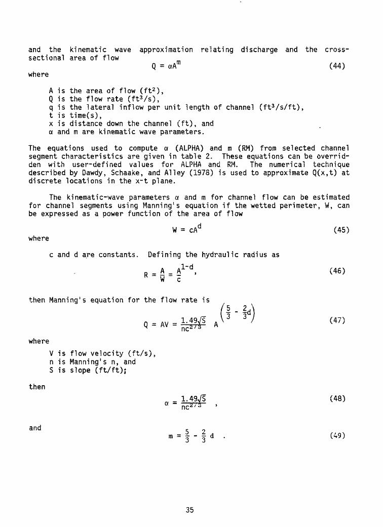
and the kinematic wave approximation relating discharge and the cross- sectional area of flow
Q = aAm (44) where
A is the area of flow (ft2 ),Q is the flow rate (ftVs),q is the lateral inflow per unit length of channel (ftVs/ft),t is time(s),x is distance down the channel (ft), anda and m are kinematic wave parameters.
The equations used to compute a (ALPHA) and m (RM) from selected channel segment characteristics are given in table 2. These equations can be overrid den with user-defined values for ALPHA and RM, The numerical technique described by Dawdy, Schaake, and Alley (1978) is used to approximate Q(x,t) at discrete locations in the x-t plane.
The kinematic-wave parameters a and m for channel flow can be estimated for channel segments using Manning's equation if the wetted perimeter, W, can be expressed as a power function of the area of flow
W = cAd (45)where
c and d are constants. Defining the hydraulic radius as
n _ A _ A1" 01 , (46)R " W " c
then Manning's equation for the flow rate is
( ^ " "3 ) 1.49^/S \ ° ° / (47)^ ~ nc2/:*
whereV is flow velocity (ft/s), n is Manning 1 s n, and S is slope (ft/ft)j
then(48)
and . 0m = - d . (49)
35

Dawdy, Schaake, and Alley (1978) suggest that the time and space steps, At and Ax, used in the numerical computations, be selected on the -frequency- response characteristic (time to equilibrium) of "fastest" channel segment, the highest expected lateral inflow rate and a unit-hydrograph rule of thumb. A linear-stability criterion (Woolhiser and others, 1970) also can be used to temper the selection of the time and space steps for channel segments with predominantly upstream flow. This criterion is
(50)
where
A is a maximum expected cross-sectional area of flow.
Reservoir Routing
Reservoir routing is based on a general form of the continuity equation:
where
= 1- (51)at
0 is reservoir outflow,I is reservoir inflow,STO is reservoir storage, andt is time.
For daily streamflow computations, I is the sum of the streamflow contribu tions from all HRU's and the part of subsurface- and ground-water reservoirs above the channel reservoir. Reservoir inflow also can include the outflow of up to 3 upstream channel reservoirs. For storm-mode computations, the reser voir is treated as an individual stream segment in the channel-routing scheme. Reservoir inflow in this case is the upstream input of any combination of up to three channel, reservoir, and junction segments.
Two types of reservoir routing are available. One is linear storage routing which uses equation 51 and the relationship
0 = RCS * STO (52)
where
RCS is a routing parameter.
Substituting equation 52 into equation 51 and rearranging terms produces
d(STO) = I - (RCS * STO) (53) at
36

Equation 53 is solved for STO, and this solution is substituted back in equation 51 producing:
-(RCS*At) 0 = (1~ 1" 8RCS*At ) * I * At + (iV (RCS*At) ) * STO, (54)
where
At is the time interval, andSTO is the reservoir storage at the start of At.
STO is recomputed at the end of each At and used in the next iteration of equation 54.
The second type of reservoir routing available is modified-Puls routing (U.S. Soil Conservation Service, 1971). In this procedure, the 0 and I terms of equation 51 are the averages of 0 and I at the beginning and end of time interval At. Rearranging equation 51 using these average values gives
2STO 2STO
where the subscripts 1 and 2 specify start and end values for time interval At. All terms on the right-hand side of equation 55 are known at the begin ning of a routing period. An interpolation procedure described by Dawdy, Schaake, and Alley (1978) is used to solve for 0/>. A table of outflow versus
-rr + 0 values is computed by the model from a user-specified table of stor
age versus outflow. 0? can be determined by entering the computed table
2STO£with the value of T-T + 0« computed from equation 55. Reservoir evapora
tion, leakage, bank storage, and inflow by direct precipitation are not accounted for by the model.
The type of routing for each reservoir is selected with varibles IRTYP for daily routing and TYPE for storm routing. IRTYP and TYPE must be the same value for a given reservoir. Reservoir routing for daily streamflow simula tion is done in subroutine RESVRD. Reservoir routing for storm events is done in subroutine RESVRU.
Sediment
Sediment detachment and transport from overland flow-planes is computed only for storms. Computations are done in subroutine UNITD. The conservation of mass equation used to describe sediment detachment and transport is one presented by Hjelmfelt, Piest, and Saxon (1975) and is expressed as:
= ER + EF (56)
37

where
c is sediment concentration, in kilograms per cubic foot(Kg/ft3 ),
h is flow depth (ft),q is flow rate per unit width (ft3 /s/ft), ER is the rainfall detachment rate of sediment (Kg/ft2 /s), EF is the overland flow detachment rate of sediment (Kg/ft2 /s),x is distance down the flow plane (ft), andt is time(s).
ER is computed using a relationship described by Smith (1976) which is ex pressed as:
ER = KR 'V PPT* * e- &C* ^ «?)
where
PPT is the rainfall rate (ft/s),HBAR is the mean depth of flow (ft), andKR and HC are parameters.
EF is computed using a relationship described by Hjelmfelt, Piest, and Saxon (1975) which is expressed as
EF = KF * (TC-TR) (58) where
TC is the sediment transport capacity (Kg/s),TR is the current sediment transport rate (Kg/s), andKF is a parameter.
TC = MM * HBAREN (59)
TC is computed by
where
MM and EN are parameters.
For a given time step, the rainfall detachment rate (ER) is added to the current transport rate (TR) and the sum is compared to the transport capacity (TC). If the sum is greater than the transport capacity, then the current transport rate is set equal to the transport capacity. If the sum is less than the transport capacity, then the flow detachment (EF) computations are made and added to the current transport rate.
Equations for overland flow are solved to obtain the appropriate values of q and h for use in equation 56. The time trace of sediment-transport rate per unit width of overland flow plane is written to a temporary disk file for use in channel-transport computations performed in subroutine ROUTE.
38

Sediment is transported as a conservative substance in the channel system; sediment detachment and deposition in the channel are not included. Channel transport is computed using the channel network described under the Channel Flow heading of this section. The continuity of mass equation used to describe sediment transport is expressed as:
= TLAT (60)
where
A is the cross-sectional area of flow (ft2 ), Q is the flow rate (ft3 /s), andTLAT is the lateral inflow rate of sediment to the channel
(Kg/s/ft).
TLAT is obtained from the temporary disk file written in subroutine UNITD.
Snow
The snow components simulate the initiation, accumulation, and depletion of a snowpack on each HRU. A snowpack is maintained and modified both on a water-equivalent basis and as a dynamic-heat reservoir. A snowpack-water balance is computed daily, and an energy balance is computed twice each day for two 12-hour periods (designated day and night). Most snow computations are done in subroutine SNOBAL.
The conceptual model for the snowpack system and its energy relationships is one described by Obled and Rosse (1977). The snowpack is assumed to be a two-layered system. The surface layer consists of the upper 3 to 5 centime ters of the snowpack, and the lower layer is the remaining snowpack. Heat transfer between the surface layer and the lower layer occurs by conduction when the temperature of the surface layer (TS) is less than 0°C (Celsius). When TS equals 0°C, heat transfer occurs as conduction when the net energy balance at the air-snow interface is negative, and as mass transfer by surface melting when the net energy balance is positive. Heat transfer from precipi tation occurs as a mass-transfer process. Conduction of heat across the soil -snow interface is assumed to be zero, since it is negligible compared to the energy exchange at the air-snow interface. The conceptual snowpack system and the components of the snowpack energy-balance equations are shown in figure 9.
Temperature of the surface layer for the daylight period is computed as the mean of the maximum and mean-daily air temperature for an HRU. For the night period, it is computed as the mean of the minimum and mean-daily air temperature for a HRU. Snow surface temperature equals 0°C when these means exceed 0°C. When the surface temperature is less than 0°C, the mean air temperature for that 12- hour period is assumed to integrate the effects of the radiation, latent heat, sensible heat, and diffusion processes expressed in the complete equation for the surface temperature. See Andersen (1968) for a complete discussion of the equation.
39

Heat of precipitation
JShortwave radiation incoming Latent and
sensible heat
Longwaveradiation
air
Longwaveradiation
snow
Longwaveradiationcanopy
Shortwave radiation reflected
ConductionA and
between layers
Conduction assumed = 0
v^-O.°o°,>-S &XSO&A&
it
Surface layer snowpack
Lower layer snowpack
Figure 9.--Components of the snowpack energy-balance equations
40

The conduction of heat between the snow surface and the lower layer of the snowpack (QCOND) is computed by:
QCOND = 2 * DEN * CS
whereV
DEN is snowpack density (g/cm3 ),CS is the specific heat of ice in calories per gram per °C
(cal/g/°C), KEFF is the effective thermal conductivity of the snowpack
(cal/s/cm/°C), At is the time interval (s), n is pi , and PACT is the temperature of the lower layer of the snowpack (°C).
KEFF is assumed equal to 0.0077 * DEN2 (Anderson, 1968). DEN is computed by:
DEN = PWEQV/DPT (62)
where
PWEQV is snowpack water equivalent (in.); and DPT is snowpack depth (in.).
DPT is computed using a finite difference scheme to solve the equation (Riley, Israelsen, and Eggleston, 1973):
+ [SETCON*DPT(t)j =
PSN SETCON ,, (63) DENI DENMX
where
SETCON is a settlement- time constant, PSN is net daily snowfall (inches water equivalent), DENI is initial density of new-fallen snow, DENMX is the assumed average maximum snowpack density, t is time in days (t=0 at date of snowpack initiation), and PSS is accumulated sum of PSN from time of snowpack initiation (in. water
equivalent),
The temperature of the lower layer of the snowpack, PACT, is recomputed each 12-hour period by:
PACT = -PKDEF ,,, . *AL1 (PWEQV*!. 27) ^ ;
41

where
PKDEF is the number of calories of heat required to bring the lower layer to an isothermal state at 0°C.
The constant 1.27 is the product of the specific heat of ice (0.5 calories/ gram'/°C) and the conversion factor for inches to centimeters (2.54).
When the temperature of the surface layer equals 0°C, an energy balance at the air-snow interface is computed. For each 12-hour period the energy balance CALN in calories is computed by:
CALM = SWN + LWN + CEN (65)
where
SWN is net shortwave radiation (cal), LWN is net longwave radiation (cal), andCEN is an approximation of the convection-condensation energy
terms (cal).
An additional energy term for the heat content of precipitation (CALPR) is computed in subroutine PRECIP and is added to the snowpack before CALN is computed.
Net shortwave radiation SWN is computed by:
SWN = SWRD * (1.0 - ALB) * TRNCF (66)
where
SWRD is the computed shortwave solar radiation received (ly), ALB is the albedo of the snowpack surface, andTRNCF is the transmission coefficient for the vegetation canopy over
the snowpack.
For albedo computations, the snowpack is considered to be in either an accumulation phase or a melt phase. A new snowpack begins in the accumulation phase and continues in this phase until the temperature of the lower layer is 0°C for 5 consecutive days or the Julian date exceeds a forcing date ISP2. At this point, the snowpack shifts to the melt phase. The date to begin checking for the start of the melt phase (ISP1) and the date to force the start of melt phase (ISP2) are user-specified. Snow surface albedo is computed as a func tion of the snowpack phase and the number of days since the last snowfall (SLST). A separate albedo-SLST relationship (U.S. Army, 1956) is used for each phase. The albedo of new snow decays daily according to the albedo-SLST relationship in effect at the time of the snowfall. The number of days since the last snowfall (SLST) is reset to zero when all-snow precipitation of at least 0.05 inches water equivalent during the accumulation phase, or 0.1 inches water equivalent during the melt phase, occurs. For precipitation that is a mixture of rain and snow, SLST is not reset if the percentage rain in the mixture (PRMX) is greater than or equal to user-defined value of RMXA for the accumulation phase or RMXM for the melt phase.
42

The transmission coefficient (TRNCF) is estimated using a winter forest- cover density (COVDNW)-TRNCF relationship for the vegetation canopy over the snowpack. Miller (1959) developed a COVDNW-TRNCF relationship for several species of pine, and Yezina and Pech (1964) developed similar relationship for both jack pine and balsam fir. Both pine relationships are shown in figure 10, with an average of the two curves that has given reasonable results in model applications (Leavesley and Striffler, 1978).
Longwave net radiation (LWN) has two components the longwave exchange between the air and snowpack surface and the longwave exchange between the vegetation canopy and the snowpack surface. LWN is computed by:
LWN = (1.0 - COVDNW) * [(EMIS*AIRN)-SNON]
+ COVDNW * (AIRN-SNON) (67)
where
COVDNW is the winter cover density of the predominantvegetation above the snowpack,
EMIS is the emissivity of air, AIRN is the longwave energy emitted from a perfect black -
body at the average air temperature for the 12-hourperiod (cal), and
SNON is the longwave energy emitted from the snowpacksurface at the surface temperature (TS) for the 12-hour period (cal).
AIRN and SNON are computed using the Stefan-Boltzmann law. The temperature used for AIRN is the average of the daily-minimum and daily-mean air tempera tures for the night period, and the average of the daily-maximum and daily-mean air temperature for the daylight period. The snowpack and the vegetation canopy are assumed to radiate as perfect black bodies and, thus, have an emissivity of 1.0. Emissivity of the air (EMIS) is a function of its moisture content and ranges between 0.757 and 1.0 (U.S. Army, 1956). For days without precipitation, EMIS is user specified as EAIR. For days with precipi tation, EMIS is computed separately for the day and night periods as a func tion of storm type and observed solar radiation. A period of months during which storms are predominantly convective in origin can be user-specified with the first month (MTSS) and last month (MTSE) parameters. Storms occurring outside these months are assumed to be frontal in origin with an associated EMIS of 1.0 for both day and night periods. During the convective storm period, days with precipitation are assumed to have an EMIS of 0.85 for the night period. For the associated day period, EMIS is assumed to vary between EAIR and 1.0 as a function of the ratio of observed to potential solar radia tion received on a horizontal surface. If solar radiation is computed from temperature data, the day period EMIS is assumed to be 1.0.
The full equation for computing latent and sensible heat flux includes terms for temperature, vapor pressure, wind speed, and diffusivities of heat and vapor (U.S. Army, 1956). However, wind and vapor pressure or humidity data generally are not available. Therefore, the full equation is simplified
43

90
80
S 70ccUJO.
^ 60UUO
cc
r so
cc
40ULu_ lit O O
O 30
20
10
\ Nfc ^x,\ . X<5>, ^ZS>~-
10 20 30 40 50 60
WINTER COVER DENSITY (COVDNW), IN PERCENT
70
Figure 10.--Functional relationships Detween winter forest-cover density (COVDNW) and the transmission coefficient (TRMCF) of the forest canopy.
44

to a temperature index form to estimate latent and sensible heat terms. It is computed by:
CEN = CECN(MO) * TAVC (68)
where
CEN is an estimate of latent and sensible heat,CECN is a parameter for month MO, andTAVC is the mean air temperature for the 12-hour period (°C).
To provide a measure of the influence of wind in the full equation for CEN, areas of forest cover are assumed to receive only one-half of CEN computed by equation 68. Vapor pressure influences are considered by computing CEN only on days of rainfall or when the ratio of observed to potential shortwave solar radiation is less than or equal to 0.33.
When the 12-hour energy balance (CALN) is negative, heat flow occurs by conduction only. The amount and direction of heat flow is computed from equation 61. When the 12-hour energy balance is positive, this energy is assumed to melt snow in the surface layer. Snowmelt transports heat into the snowpack by mass transfer. Sncwmelt and subsequent thermal and water equiva lent changes in the snowpack are computed in subroutine CALIN. Snowmelt (SMLT) is computed by:
SMLT = ^r- (69)
where
203.2 is the number of calories required to melt 1 inch of water- equivalent ice at 0°C.
If the temperature of the lower snowpack (PACT) is less than 0°C, then part or all of the snowmelt is refrozen, releasing 203.2 calories per inch of snowmelt refrozen. This heat is used to satisfy part or all of the heat deficit in the lower snowpack (PKDEF), and a new temperature is computed for the lower snowpack using equation 64. When the temperature of the lower snowpack reaches 0°C, any additional snowmelt is used to satisfy the free water-holding capacity (FWCAP) of the snowpack. FWCAP ranges from 2 to 5 percent of the water equivalent of the snowpack existing in the ice phase (U.S. Army, 1956; Leaf, 1966) and is user-specified. Once FWCAP is satisfied, the remaining snowmelt moves out of the snowpack and becomes available for infiltration and surface runoff.
When the temperature of the lower snowpack is 0°C and the surface temper ature is less than 0°C, heat is conducted from the lower snowpack to the snowpack surface. The amount of heat conducted to the surface is computed using equation 61. The heat loss from the lower snowpack first causes any FREWT held in the pack to freeze. The calorie loss (CALND) required to freeze the FREWT is computed by:
CALND = FREWT * 203.2 (70)
45

Any loss available after FREWT is frozen is accumulated as a heat deficit in variable PKDEF, and a new temperature for the lower snowpack is computed using equation 64. These computations are done in subroutine CALOSS.
Evaporation and sublimation from the snow surface are assumed to occur only when there is no transpiration occurring from vegetation above the snowpack. The loss from the snow surface (SNEV) is computed daily as a percentage of the potential evapotranspiration (PET) value computed in subrou tine PETS. The equation used is:
SNEV = (CTW*PET) - XINLOS (CTW*PET) > XINLOS (71) SNEV = 0 otherwise;
where
CTW is a loss coefficient, andXINLOS is the evaporation and sublimation loss from interception
computed in subroutine INTLOS (in.).
Optimization
This component controls the automatic adjustment of a specified set of parameters (NV in number) to obtain better agreement between observed and predicted runoff, a process known as optimization. The user selects the parameters to be adjusted by specifying the parameter numbers in an array LOP(J), J=l,2,... ,iMV. The parameters and their corresponding numbers are given in table 3. A maximum of 20 parameters may be adjusted during an optimization run, or NV^2Q. The capability to optimize 20 parameters is not provided to encourage the optimization of a large number of parameters. Rather, it is provided to permit a sensitivity analysis of many parameters. This capability is discussed in the Sensitivity Analysis section of this report.
The agreement between observed and predicted runoff is measured by an objective function. The optimization attempts to adjust the parameters to minimize the value of the objective function. The user specifies whether the objective function is to be computed using daily runoff volumes (IOPT=1 or 2), storm volumes (IOPT=3), storm peaks (IOPT=4), or storm volumes and peaks simultaneously (IOPT=5 ; see section Optimization Using Peaks and Volumes Simultaneously). If daily volumes are used, setting IOPT=2 allows the corre lations between the daily runoff prediction errors to be modeled as a station ary time series (see section Correlated Daily Errors); if IOPT=1, no correlation is assumed. When IOPT is either 1 or 2, the user must specify the months within each year (month NFS through month MFN, inclusive) to be includ ed in computation of the daily objective functions. When IOPT is 3, 4, or 5, the model must be run in the storm mode, and the user must specify the storms (TESTNO(J), J=l,2,...,NST, where NST is the number of storms) to be included in computation of the objective function.
The objective function when IOPT is 1, 3, or 4 is computed in one of two ways; it is the sum either of the squared differences (IOBF=2) or of the absolute differences (IOBF=1) between the observed and predicted runoff values. Logarithms (natural) of the runoff values can be used for computing
46

Table 3. Model parameters and the associated values of the array, LOP
Parameter identifi cation No.
(LOP)
12345
6789
10
1112131415
1617181920
21
222324
2526272829
30
Number of parameter elements
NRUNRUNRUNRUNRU
NRUNRUNRUNRUNRU
NRUNRUNRUNRUNRU
NRUNRUNRUNRUNRU
NRU
NRUNRUNRU
NRUNRUNRUNRUNRU
NRU
Parameter
COVDNSCOVDNWTRNCFSNSTCTX
TXAJTNAJSMAXREMXSRX
sexSCNRNSTSRNSTWKSAT
PSPDRNRGFNOT USEDD50
KR
HCKFKM
ENSCISEPDRCORDSCOR
TST
Parameter identifi cation No.
(LOP)
5051525354
6061707172
7374757680
8185869091
9293949596
979899
100101
102103
Number of parameter elements
NRESNRESNRESNRESNRES
NGWNGW121212
12121212NOFSEG
NOFSEGNCRSEGNCRSEG121
11111
11111
11
Parameter
RCFRCPRSEPRESMXREXP
RGBGSNKTLXTLNRDM
RDCEVCPATCECNALPHA
RMALPHACRMCCTSNOT USED
BSTSETCONPARSPARWCSEL
RMXARMXMCTWEAIRFWCAP
DENIDENMX
47

either objective function if ITRANS is set to 1; otherwise, ITRANS is 0. When IOPT is 1 or 2 and ITRANS is 1, one is added to the daily runoff values before logarithms are taken to avoid taking the logarithm of zero. When IOPT is 2 or 5, a special form of the objective function is used, as described in following sections.
There are two algorithms available for performing an optimization: the Rosenbrock and the Gauss-Newton routines. To use the latter, the value of IOPT as described above is made negative; if IOPT is positive, the Rosenbrock routine is used.
The user has the option of running the model for a period of time before the optimization process is begun. When this is done, the beginning and ending dates for the initialization period (BYRIN/BMOIN/BDYIN and EYRIN/EMOIN/ EDYIN) and for the optimization period (BYROP/BMOOP/BDYOP and EYROP/EMOOP/ EDYOP) must be specified. If no initialization period is desired, BYRIN is set to 0. The optimization period always must begin immediately after the initialization period ends. Several optimizations may be performed simply by placing the data for each in succession at the proper point in the data deck (see input data instructions).
Rosenbrock OptimizationThe Rosenbrock optimization technique is described in detail in a paper
by Rosenbrock (1960) and is discussed in a hydro!ogic context by Dawdy and O'Donnell (1965) and Dawdy, Lichty, and Bergmann (1972).
The parameter adjustment proceeds by stages. During the first stage, each parameter represents one axis in an orthogonal set of NV search directions. Adjustments are made in these search directions until arbitrary end-of-stage criteria are satisfied. Then another stage is begun by computing a new set of NV orthogonal search directions based on the experience of parameter movement during the preceding stage. This process is repeated and continues until convergence has occurred or until a specified number of adjustments (NV x NTRY, where NTRY is the number of adjustments per parameter) has been tried. The major feature of this procedure is that, after the first stage, one axis is alined in a direction reflecting the net parameter movement experienced during the previous stage.
To start the fitting process, the model is assigned an initial set of parameter values and upper (HU) and lower (GU) bounds for each parameter. The model is run, and the objective function (OBF) is calculated and stored as a reference value. A step of user-specified length (a proportion P of the parameter magnitude) is attempted in the first search direction, and the model is run again with the adjusted parameter value. If the resulting value of the objective function is less than or equal to the reference value, the trial is registered as a success, and the appropriate step size for each parameter is multiplied by 3 for the next adjustment along this axis. If a failure results, the step is not allowed and the step size is multiplied by -1/2. That is, the next adjustment along this search axis will be in the opposite direction and only one-half the magnitude of the current adjustment. An attempt is made in the next search direction and the process continues until the end-of-stage criteria are met. At this point, a new orthogonal search
48

pattern is determined and another stage of optimization undertaken. The
objective-function value and associated parameter values are printed for each trial .
Gauss-Newton Optimization
The Gauss-Newton optimization algorithm essentially is identical to the linearization method described by Draper and Smith (1966, p. 267-270) and by Beck and Arnold (1977, p. 340-349), and in addition incorporates the Box-Kanemasu interpolation modification (see Beck and Arnold, 1977, p. 362-368).
~(k} Let pv J be the set of NV parameter values obtained at the k-th iterationof the routine; the (k+l)th set is then computed by
(72)
where
(k) _ -IT_
The NV x 1 vector c v ' is the parameter correction vector, and \r ' is a
scalar multiplier that is equal to one in the ordinary Gauss-Newton algorithm.The matrix A=(a. .) is the sensitivity matrix, and Z=(z..)=AA is the,information matrix (described in the section Sensitivity Analysis Components),
-Ck) both evaluated at p . The superscript T denotes transpose and thesuperscript -1 denotes inverse. The vectors 0 and P are observed and predict-
~(k} ed runoff, the latter computed with parameters p .
The correction vector at each iteration is found by a call to subroutine
SENST, which performs a partial sensitivity analysis to obtain the magnitude( k") and direction of c^ . The multiplier h vis ' initially is 1 for each iteration.
If the resulting parameters p^ ^ are outside the constraints imposed by theCO user, hr ' then is halved repeatedly until all values lie within the
constraints. Next, if the objective function obtained with parameters p ' is not smaller than that with p^ , the scalar fr ^ again is halved until the objective function shows some improvement. At this point, the Box-Kanemasu
interpolation scheme is used to obtain a final value for h
49

As in the Rosenbrock optimization, the initial parameter values fr ' are
those assigned by the user in the input data. Iterations continue until the-Ck+1) - (k} elements of p v J differ from those in [S by a small percentage, or until
the number of iterations exceeds NTRY, whichever comes first.
Distributed Parameters
Distributed parameters are defined to be those that are a function of hydrologic response unit, of subsurface reservoir, of ground-water reservoir, of overland flow-plane or channel segment, or of time. Optimization of these parameters presents a special problem because the number of elements over which a parameter is distributed typically is large, and because the observed runoff values used in an optimization are the responses from all the elements lumped together. These two factors make changes in predicted runoff because of changes in any particular element difficult to detect; that is, sensitivi ties to changes in the individual elements are apt to be small.
The model provides two options for dealing with these problems, both of which actually are just ways of constraining the optimization. Consider, for example, adjustment of the parameter COVDNW. There actually are NRU hydrolog ic response units (HRU's) into which the basin has been divided; thus, there are NRU values of this parameter. If there are a large number of HRU's, it probably is not feasible to adjust the NRU values of COVDNW independently. Thus, the user is provided with the option of constraining the optimization so the NRU values are all adjusted in the same direction. Initial values of COVDNW for each of the NRU HRU's are user-specified. The user then may elect to adjust these NRU values, or any subset of these values, (1) by the same magnitude or (2) by the same percentage of the initial value. A variable ILOPL must be specified for each parameter to be optimized. If the user wishes to adjust a parameter using option (1) above, ILOPL is set to 0; if option (2) is to be used, ILOPL=1.
Also, variables NVAR and NDVR must be specified for each parameter. The number of values of a distributed parameter that are to be adjusted together is NVAR. For the parameter COVDNW, for example, NVAR would be NRU if it is desired to adjust all COVDNW values together; or, NVAR could be less than NRU if it is desired to adjust only a subset of the COVDNW values. The numbers of the elements on which a distributed parameter is to be adjusted are specified by the values NDVR(.,J), J=l,2,..., NVAR. For example, if COVDNW is defined on a watershed with five HRU's (NRU=5), and it is desired to optimize the values only on even-numbered units, leaving the value on odd-numbered HRU's unchanged, then NVAR=2, NDVR(.,1)=2, NDVR(.,2)=4.
The program also allows one to adjust different subsets of distributed parameter values independently. In the example in the preceding paragraph, if one wished to adjust COVDNW on even-numbered HRU's and COVDNW on odd-numbered HRU's independently, the NVAR and NDVR for the former would be as given above, and for the latter, NVAR=3 and NDVR(.,!)=!, NDVR(.,2)=3, NDVR(.,3)=5. As a special case of this, the values on all HRU's may be adjusted independently.
50

Optimization instructions for parameters distributed over subsurface reservoir, ground-water reservoir, flow segment, or time are specified in an analogous manner. The variable NVAR must always be less than or equal to the maximum number of parameter elements (table 3) for a given distributed parame ter configuration. For parameters that are not distributed, NVAR is set to 1.
When adjustments according to option (1) are to be performed, the program first calculates an average parameter value (XXAVE). For example, XXAVE for COVDNW is calculated by:
XXAVE = I COVDNW(J)/NRUJ .L
if all NRU values are to be adjusted. Adjustments are then made on XXAVE; deviations from the average, XXDEV, are kept constant. Thus, although there are a total of NRU parameters, there are also NRU-1 linear constraints, resulting in only one parameter being adjusted.
On the other hand, adjustments of the same percentage [option (2)] are made by first transforming the parameters, and then using the same procedure involving XXAVE and XXDEV on the transformed values. The transformed parame ters are calculated by taking the natural logarithm of the original value plus 20. Due to the logarithmic transformation, linear changes in the transformed parameters are equivalent to multiplicative changes in the original parame ters. The constant 20 is added to keep the transformed values positive.
Correlated Daily Errors
When performing an optimization or sensitivity analysis using daily runoff predictions, the user may elect (by setting IOPT=±2 or ISEN=2) to include an analysis of the error correlations. It is recommended that this option be used whenever a daily optimization is performed; parameter estimates so obtained are likely to be more physically reasonable, and prediction errors in noncalibration periods usually will be smaller. Correlated errors are discussed by Beck and Arnold (1977) and, in a rainfall -runoff modeling con text, by Sorooshian and Dracup (1980).
The error structure is assumed to be of the form°i = p i + ei-where
0. and P. are the observed and predicted runoff, and
e. is the prediction error, for the i-th day.
In the usual least-squares optimization, the objective function 1(0. -P.)2 is minimized. This is equivalent to obtaining maximum likelihood parameter estimates with errors e. that have a normal distribution and are uncorrelated with each other. In a 1 daily optimization, the assumption of no correlation
51

among the errors e. is clearly violated; the correlation between errors 1 day apart (lag-one correlation) typically will be greater than 0.9, and the correlation between errors K days apart (lag-K correlation) decreases rather slowly as a function of K. This fact should be incorporated in doing an optimization.
The correlation of the errors is modeled by fitting an autoregressive- moving average (ARMA) time-series structure (see Box and Jenkins, 1976); that is, it is assumed that the errors e- obey a model of the form
v «i ei-i--"- VI-P^ -elfV:L -...-eqVq. (74)
This model is said to be a mixed ARMA model of order (p,q). The {n.} sequence is a zero-mean white noise process, and $., 0. are parameters that are estimated by the optimization routine along with the physical model parame ters. The user must specify the orders p and q.
As an example, when p=l and q=0, the parameters are found by minimizing the following objective function:
U = I [0. - (j>1 O i . 1 - (P. - ^ P^)]2 (75)
The predicted runoffs P. and P._-, here are a function of the physical parameters. When $- = 0, this reduces to the ordinary least-squares objective function. For more general p and q, see Beck and Arnold (1977).
Constraints (Prior Information)
For both the Rosenbrock and Gauss-Newton optimization schemes, lower and upper bounds outside which the parameters cannot be adjusted must be speci fied. It should be noted that if the minimum of the objective function for this constrained optimization is located at one of the boundaries, the Gauss-Newton routine usually will not perform satisfactorily in finding this minimum; it is recommended that the Rosenbrock algorithm be used in this case. Also, an optimization may be made essentially unconstrained if the specific bounds are made sufficiently wide.
Lower and upper bounds on the parameters are equivalent to what is known as a uniform (or rectangular) prior-probability distribution on the parame ters. (See Beck and Arnold, 1977.) That is, it is known before the optimiza tion that the parameters fall somewhere within the range given, but nothing is known regarding where within this range of values the true parameters lie.
As an alternative to the uniform prior-probability distribution the user may specify a prior distribution that is normal by setting IPRIOR=1. Thus, prior knowledge about the true parameter values is assumed to be better represented by a bell-shaped normal distribution than by a rectangular-shaped distribution. The most likely true value of the parameter (that is, the mean of the prior distribution) is that specified in the data input, with the likelihood of the value decreasing as distance from the mean increases. The
52

tightness of the constraint with a normal prior is defined by user specifica tion of the variance (standard deviation squared) of the distribution. As a rough guide to determining the standard deviation, it should be recalled that about 95 percent of the area under a normal curve lies within two standard deviations of the mean.
The normal distribution alternative is useful for another reason. One may incorporate knowledge not only about the likely values of the parameters individually, but also about how parameters are presumed to be related to each other. This is done by specifying the correlations between each pair of parameters. (The parameters taken together are taken to have a multivariate normal prior.) A correlation of ±1 between a pair of parameters would signify a direct linear relationship between the two; in practice, however, all correlations must be given as less than one. It is recalled that the user is given the option of specifying linear constraints among values of a distrib uted parameter by proceeding as described in the section Distributed Parame ters. The use of the normal prior information option, on the other hand, would allow one to place somewhat weaker constraints on distributed parame ters, if desired.
The objective function for normal prior information is:
U = [Z(0.-P.)2] exp [({3-H)T V" 1 (p- M )/n] (76)
where
p is the vector of parameters being optimized, and u and V are the user-supplied mean and covariance of the
prior distribution.
Note that, as the constraints become looser, the elements of V become larger and U approaches an ordinary least-squares objective function. As mentioned before, the elements of jj are the user-specified parameter values in the data input. The elements of V are given as input (array VB) in Card Group 7. One row of V is on each card. For example, if for two parameters (NV=2)
"l.O 1.5
V = 1.5 3.0
the first card would have values (1.0, 1.5) and the second card would have (1.5, 3.0). The diagonal elements 1.0 and 3.0 are the parameter variances and 1.5 is the covariance between the two parameters. The correlation is:
^ = 0.87..O)] 2
Optimization Using Volumes and Peaks Simultaneously
Setting IOPT-±5 allows optimization using flood peaks and volumes simul taneously. The estimation procedure is maximum likelihood, under the assump tion that volume errors and peak errors have a bivariate normal
53

distribution (see, for example, Hiemstra and Francis, 1981) with zero means and covariance matrix that is estimated along with the physical parameters. The objective function that is minimized is-:
where
U = IE2 I2 - (I E E ) 2 (77)^~ l / ^~r\ ^ ̂~ / r\ * \. * J
E is observed minus predicted volume, andE is observed minus predicted peak, and the summation is over the P n storms.
The covariance between peak errors and volume errors is estimated by
n IE E . and the variances are n IE 2 and n IE 2 , so U may be expressed v p v p
as:U = IE 2 IE 2 (1 - r 2 ) , v p ' (78)
letting r be the sample correlation between peak and volume errors.
Use of this option permits optimization on parameters that influence both volumes and peaks simultaneously. Individual parameters may influence both, and there may be parameters that influence one but not the other. The form of the objective function automatically sorts out sensitivity of both model responses with respect to changes in each parameter, giving each parameter an appropriate influence on the value of U. For example, if one were to use this option with parameters that had no influence on volumes, the optimization would be equivalent to a least-squares fit using peaks.
Statistical Analysis
Daily Error Summaries
Several error summaries are available to aid the user in comparing observed and predicted runoff. At the end of each month, a table summarizing the errors for that month is printed. In the first row of that table, four objective function values are given:
Ie 2 , and
where
e = 0-P,
0 = observed runoff, and P = predicted runoff.
54

The quantity e is the error, or residual, associated with the daily predic tion, and ̂ e, is the error in log-transformed daily prediction. The cumulative sums of these values for month NFS through month MFN (see Optimization Sec tion) are given in the next row of the table. Then, mean values obtained by dividing the objective function by the number of days in the month are print ed. Finally, these means expressed as a percentage of the mean observed runoff for the month are given for the untransformed runoff. For the Ie2 objective function, the percentage is obtained by first taking the square root of the mean objective function (yielding a "standard error"), then dividing by the mean observed runoff.
By setting ISTAT equal to 1 on the "PRINT-OP" input card (card 7, Card Group 1), the user may obtain a statistical summary for the entire period of record. First, a table showing monthly total and mean runoff, both observed and predicted, is given. The number of positive and negative residuals and the total number of positive and negative runs in the residuals also are shown month by month. A positive run is defined to be a sequence of positive residuals, preceded and followed by a negative residual, and a negative run is defined analogously. These quantities also are shown for each year and for the total period.
In addition, setting ISTAT=1 results in the following statistics being computed for both the total period and the MFS-to-MFN season:
coefficient of determination^ - Ie2 /Ie..2 ;coefficient of persistence=(r-m)/s;coefficient of gain from daily averages=l - Ie2 /IeD2 ;
coefficient of correlation between predicted and residualrunoff=I(eL-eL)(PL-PL)/[I(eL-iL ) 2
wheree=0-P,
0=mean observed runoff for full period of simulation,
r=total number of runs,
m=mean number of runs, and
s=standard deviation of number of runs under the hypothesis thatthe order of signs of the residuals is random (Weeks and Hebbert,
1980), eD=0 - V
0 =mean value for that day of the year,
55

e L=ln(0+l) -
e. =mean of e, ' s,
P L=ln(P+l),
P=mean of PT ' s .Li Li
Finally, when ISTAT=1, a table is given showing suras le, le, , IL
, Ze 2 , le 2 , means of these values, and these means expressed as a percent Liof mean observed runoff. This table is given for both total period and
MFS-MFN season.
The coefficient of determination is equivalent to R2 for a regression analysis. It is always between 0 and 1 and measures the fraction of the total runoff variation (Ie) explained by using the model.
Ideally, one wants to obtain mean errors near zero with mean absolute errors and mean squared errors as small as possible. The mean error, together with the table giving the number of positive and negative residuals, tells the user whether the model seems to be consistently overpredicting or underpredicting. The correlation coefficient between residual and predicted values tells whether there is any consistent association between these two variables; a positive correlation signifies that e=0-P is large when P is large, or that the model generally is underpredicting for large events and overpredicting for small events. This problem may result from model error, input error, parameter error, or a combination of these; the user must decide whether it is desirable or possible to reduce parameter error by an optimiza tion (parameter adjustment) procedure.
The coefficient of persistence measures the serial correlation, or persistence, in the residuals. A highly negative value indicates a large degree of persistence, or tendency for positive errors to follow positive errors and negative errors to follow negative errors. The coefficient of persistence is standardized so that under the hypothesis that the order of signs of residuals is random, it is distributed for large samples as a stan dard normal random variable. The significance of the computed coefficient can be determined from a standard normal table. For example, the probability that a standard normal random variable is -1.65 or less is 0.05. Therefore, if the computed coefficient is less than -1.65, it is unlikely that the order of the signs is random. Thus, there is significant persistence.
The coefficient of gain from daily averages compares model predictions to predictions based solely on means for each day of the year. For example, the daily average prediction for July 1, given 4 years of record, would be the mean of the four observations for that date. The coefficient is between 0 and 1; a value closer to 1 indicates better predictions using the model over the daily average predictions.
56

Storm Error Summaries
When the model is run with storm data, a table showing
Ie 2 , Ie 2 is given, where e=Q-P and e,.=lnO - InP are now computed with storm
volumes (in inches). If routing is performed, these error measures also are
given for storm peaks. The mean values of these objective functions, and
these means as a percentage of the mean observed values, also are printed.
Sensitivity Analysis
These subroutines perform a sensitivity analysis on the parameters of the model. The results of this analysis allow the user to determine the extent to which uncertainty in the parameters results in uncertainty in the predicted runoff, and to assess the magnitude of parameter errors and parameter intercorrelations when an optimization is performed. Complete discussions of interpretation of the output of the sensitivity analysis are given by Mein and
Brown (1978) and Beck and Arnold (1977).
The user selects the parameters to be analyzed by specification of the parameter numbers in array LOP(J), J=l,..., NV. The parameters and the corresponding parameter numbers are given in table 3. Variables NVAR and NDVR must be specified for a sensitivity analysis; they are interpreted exactly as those variables in an optimization and are discussed in the Optimization Components section. A sensitivity analysis of daily runoff parameters normal
ly is run separately from a sensitivity analysis of storm runoff parameters.
Let n denote the number of days (events) under consideration, and let P.
denote the predicted runoff volume for the ith day (event) l^i^n. First, a matrix with n rows and p columns (where p is the number of parameters), known as the sensitivity matrix, is computed. The element in the ith row and jth column of this matrix is a..=3P./ap.U. This notation indicates that the
partial derivative is evaluated at p, where p is the vector of parameters values used for the model run. The jth component of the vector (3 is denoted
byi^.
57

These partial derivatives are approximated by running the model firstwith parameter value S., and then again with parameter p. + Ap., where Ap. is
_ «j j j ja small fraction of p.. The quantity aP./3p.| B is approximated by the change
_ J ' J Pin P. divided by Ap.. The increment Ap. is taken to be a user-specifiedquantity (PINC) multiplied by p..
j The quantities a., are known as "absolute" sensitivities (McCuen, 1973).
Comparison of these values for different parameters is difficult because the magnitude is highly dependent on the magnitude of the parameter value itself.Therefore, dimensionless "relative" sensitivities a 1 ., are displayed, where
- "a'..=a.. (§./?.). For example, if a'..=1.40, a 10-percent change in theparameter value would produce a 14-percent change in predicted runoff.
Next, a matrix Z with p rows and p columns, known as the (scaled) infor mation matrix, is computed. This matrix is the transpose of the sensitivity matrix times the sensitivity matrix itself, so the element in the ith row and jth column is z..=I,a. .a. .. The extent to which parameter uncertainty is, on
the average, propagated to uncertainty in runoff prediction is examined by evaluating d^z^. (App2 for AJJ^kp., k=0.05, 0.10, 0.20, and 0.50, where 2..=Zz../n is an average squared sensitivity. The results are displayed as an error propagation table which gives d- for the four values of k and for each of the parameters under consideration. For example, in the column labeled 10 percent (k=0.10), a value of 150. would mean that a 10-percent error in the given parameter results in an increase of 150. in the mean squared error of prediction for the model. Units of the values in the table depend on the mode
in which the model is being run (daily or unit) and on whether runoff is being logarithmically transformed (as indicated by the switch 1TRANS). For example, in a daily mode with no logarithmic transform, the units of the value 150. above would be cubic feet per second squared (cfs2 ). In any case, the values
in the table should be compared to the mean squared error of prediction (a residual variance) a2 as defined below.
With correlated daily errors (!SEN=2), the matrix Z is computed as the transpose of the sensitivity matrix times the inverse of the estimated error correlation matrix times the sensitivity matrix. With normal prior informa tion on the parameters (IPRIOR=1), Z is altered by adding the inverse of the
user-specified parameter covariance matrix divided by a2 , defined below. (See
Beck and Arnold, 1977, section 6.6.)
58

When the parameter estimates are obtained by optimization, the covariance matrix of these estimates may be approximated using asymptotic nonlinear regression theory. When a least squares optimization is performed (IOBF=2),
this covariance matrix is the product of the inverse of Z and the scalar a2 , the residual variance. The residual variance is taken to be the squared difference objective function divided by n-p; this variance and its square root (that is, the residual standard error, a) are printed. For the minimum absolute deviation estimates (IOBF=1) the covariance matrix is obtained as when IOBF=2 except a2 is replaced by the scalar w2 , the estimated asymptotic variance of the sample median from samples having the given error distribution (see Bassett and Koenker, 1978). The variance w2 is computed by
w2=(2f)-1
where f, an estimate of the error density at the median, is given by [2(e 7 r - e ps^" 1 * en being the qth percentile of the sample of errors (see Sen, 1968).
The parameter standard errors s. and correlation matrix (c..) are then readilyJ ' J
obtainable from the resulting parameter covariance matrix, and are printed. If the parameter standard error obtained from the covariance matrix TS
referred to as a "joint" standard error, an "individual" standard error for-i*
p. is computed by s.=(z..) s, where s=a if IQBF=2 and s=w if IOBF=1. (This j j j j
actually is the standard error of J3. conditioned on given values of the otherj
parameter estimates, or the standard error that would be obtained if p. aloneJ
were being optimized.)The parameter standard errors give an idea of the uncertainty in the
optimized parameter estimates. Results of an optimization may conveniently be
given in the form "parameter estimate ± standard error." The parameter correlations give an indication of parameter interaction. A positive correla tion between two parameters means that an increase in one parameter has the
same effect on predicted runoff as an increase in the other parameter. A negative correlation means they have opposite effects on predicted runoff.
Finally a matrix known as the "HAT" matrix is computed as a product of three matrices: sensitivity matrix, inverse of the information matrix, and the transpose of the sensitivity matrix. The diagonal elements (h.) of this
matrix are printed. These values, which must all lie between 0 and 1, give an
59

indication of the relative influence of a day or a storm on an optimization. Values closer to 1 signify greater influence. A complete discussion of the interpretation of the HAT matrix is given by Hoaglin and Welsch (1978).
The variables referred to above, and the corresponding computer program names, are summarized in table 4.
Table 4. Major variables used in sensitivity-analysis components
VariableComputer variable Description
P i
N0BF
NV
0BF
ith predicted runoff volume
ith observed runoff volume
number of variables in objective function
number of parameters
objective function
n-p
a. .=
RESVAR residual variance
RESTD residual standard error
Z0PT(J) jth parameter estimate
ASENS(I,J) (i,j)th element of sensitivity matrix
ZINFC(I,J) (i,j)th element of information matrix
S j
h.
PARSTD(J) estimated ("joint") standard error of jth parameter
PARSTD(J) estimated ("individual") standard error of jth parameter
ZINV(I,J) estimated correlation between ith and jth parameters
PDENT(I) ith diagonal element of "HAT" matrix
60
Data Handling
The data-handling components input basin characteristics, meteorologic, and hydrologic data, conduct general housekeeping functions on these data, and generate model output in tabular and graphic forms. Subroutines DATIN, INVIN, DVRETR, and UVRET provide data input capabilities. Subroutines SUMALL, PRTHYD, DVPLOT, and UVPLOT provide simulation output capabilities. More detailed descriptions of input data specifications and output options are described in sections Control and System Input Specifications, and System Output.
LINKAGE OF SYSTEM LIBRARY COMPONENTS
The PRMS system library subroutine MAIN controls the sequencing and timing of model operations. Control is accomplished through a logical se quence of subroutine CALL statements to perform data initialization and input, hydro!ogic-component simulation, and output summarization. Knowledge of the structure and operation of MAIN, and of the library components called, is required to fully understand model logic and to make model modifications.
The following is a brief discussion of MAIN, the subroutine calling sequence, and data links established between library subroutines. A flow chart of MAIN is shown in figure 11. The version of MAIN discussed here is the one used in the PRMS catalog-procedure, PRMODEL. PRMODEL uses all the subroutines in the PRMS system library; table 5 is an annotated list of these subroutines. The names in parentheses in the following discussion are the subroutines called to perform the functions described.
The first functions performed in MAIN are the input of all initialization and basin descriptive data (DATIN, INVIN). In INVIN a number of disk data files are initialized or established for use in storage and transfer of data for stormflow computations. These files are listed in table 6. Next a check is made to determine if the current run is an optimization (ROSOPT), sensitiv ity analysis (SENST), or straight simulation. After all data, parameter, and variable initialization is completed, the timing structure of the model is initialized. The timing structure is a set of 3 nested DO-loops. The outer loop is incremented on water years. Within this loop, 1 water year of daily data for all meteorologic and hydrologic driving variables is input to the model (DVRETR). These daily data are stored in core. In addition, all water year counters and variables are initialized (TIMEY). The next loop is incre mented on months. When a full year of data is available, the period runs from October to September. In this loop, all monthly counters and variables are initialized (TIMEY). The inner loop is incremented on days. It is within the day loop that all hydrologic computations are made.
The first function within the day loop is to increment the counters for the Julian date JLDY, water-year date JWDY, and solar-year date JSOL. The meteorologic data for this date are then obtained. Temperature and solar- radiation data are adjusted for application on each HRU, based on differences in elevation, slope, and aspect between the climate station and each HRU (TEMP, SOLRAD). The adjusted data then are used to compute a potential evapotranspiration value for each HRU (PETS).
61

START
-Call-
DATIN
Begin __ _ year loop
Begin __ __ month loop
Begin __ day loop
Incrementday
counters
Set dailyrneteoro logic
data
Set dailyprecipdata
Figure 11. Flow chart of the MAIN program.
62

-Call- PRECIP
, yes .
yes
yes
^ yes a -Call-
INTLOS
Endmonth and day
loop
End year loop
-Call-
SUMUNTyes
10PT ISEN>
no
yes * -Call-
DVPLOT
STOP )
> yes ?
u
-Cail- PRTHYD UVPLOT
yes ^ -Call-
ROUTE
Figure 11.--Flow chart of the MAIN program Continued.
63

Table 5.--List of subroutines included in cataloged procedure PRtlODEL
SubroutineCalling subroutine Description
Daily components:
BASFLW MAIN
CALIN
CALOSS
INTLOS
PETS
PKADJ
PRECIP
RESVRD
SMBAL
SNOBAL
SOLRAD
SOLTAB
SRFRO
SUMALL
TEMP
SNOBAL PRECIP
SNOBAL PRECIP
MAIN
MAIN
MAIN
MAIN
SUMALL
MAIN
MAIN
MAIN
DATIN
PRECIP SMBAL
MAIN DATIN
MAIN
Computes baseflow and subsurface flow components of the streamflow hydrograph.
Computes change in snowpack when a net gain in heat energy has occurred.
Computes change in snowpack when a net loss in heat energy has occurred.
Computes the evaporation and sublimation of intercepted rain and snow.
Computes daily estimate of potential evapotran- spiration.
Adjusts snowpack water equivalent based on snowcourse data.
Computes precipitation form, total precipitation depth, depth intercepted by vegetation and the net precipitation.
Performs daily routing for surface-water detention reservoirs.
Performs daily soil-moisture accounting.
Computes snowpack energy balance.
Computes daily incoming shortwave solar radiation for each HRU.
Computes potential solar radiation and daylight hours for radiation planes.
Computes daily storm runoff from rainfall.
Computes daily, monthly, and annual data summaries for total basin and individual HRU's.
Adjusts daily maximum and minimum air temperature to account for differences in elevation and aspect from point of measurement to each HRU.
64

Table 5. List of subroutines included in cataloged procedurePRMODEZr-Conti nued
SubroutineCalling subroutine Description
Daily components: TIMEY MAIN
Storm components: AM INVIN
RESVRU
ROUTE
UNITD
UNSM
ROUTE
MAIN
MAIN
UNITD
Optimization components
BDRY SUB! '
COROPT
OPINIT
PARAM
ROSOPT
ROSOPT
ROSOPT
ROSOPT
MAIN
SCALE
SNORT
SUB1
SUBS
Performs initialization and maintenance of the time accounting variables.
Computes kinematic routing parameters a and m.
Performs storm-period routing for surface- water detention reservoirs.
Performs channel routing of water and sediment
Computes rainfall excess and performs overland flow routing of water and sediment.
Performs subsurface and ground-water reservoir routing for storms.
Determines whether any of the parameters being optimized lie close to their boundaries and penalizes the objective function if they do.
Performs a correlation analysis of the residuals in a daily optimization.
Reads input data and initializes variables for optimization.
Adjusts selected model parameters at thebeginning of each parameter fitting iteration.
Initializes model variables and selected model parameters at the beginning of each parameter fitting iteration.
Scales parameter and constraint values and unseales parameter and constraint values.
Determines which of new search directions is most parallel to each of the old directions following an end of stage.
65

Table 5.--List of subroutines included in cataloged procedurePRMODEL Conti nued
SubroutineCalling subroutine Description
SUB!
SUB3
ROSOPT
SUB!
Controls the main strategy of the Rosenbrock optimization procedure.
Does Gram-Schmidt orthogonalization to establish new orthogonal search directions.
Sensitivity analysis components:
MATINV
OPINIT
SENMAT
SENST
PARAM
SENST
SENST
SENST
MAIN
OPINIT
Performs matrix inversion.Reads input data and initializes variables for
a sensitivity analysis.Computes the sensitivity matrix.Controls the main strategy of the sensitivity
analysis procedure.Adjusts selected model parameters for use in
sensitivity analysis routines.
Statistical analysis components:STATS SUMUNT
SUMUNT MAIN
Data handling components: BLKDATDATIN
DVPLOT
DVRETR
INVIN
PRTHYD
UVPLOT
UVRET
MAIN
MAIN
MAIN
MAIN
MAIN
MAIN
INVIN
Computes daily statistics. Computes summary statistics.
Initializes data for common areas.Reads input of model options, parameters,
and variables.Provides line printer plot of predicted and
observed daily mean streamflow.Selects required daily records from ISAM file.
Reads input data for storm periods and handles accounting for storms.
Provides tabular output of stormflow hydrograph.
Provides line printer plot of predicted and observed stormflow hydrographs and sediment concentration graphs.
Selects required storm records from ISAM file.
66

Table 6. Data files developed in subroutine INVIN for stormflow-bydrograph computations
File name Remarks
INV Inventory of storm rainfall data by water year.FHS Hydrograph separation information for each storm period.DFHS Hydrograph separation information for each storm day.UNITP Rainfall data for each rain gage for each storm day.UNITQ Discharge data for each storm period.LATIN Direct access file used to store lateral and upstream
inflow of water (ISIM=2) and sediment (ISIM=3)to channel segments.
A check is then made to see if this date is a storm-mode simulation date. If it is, then infiltration and rainfall excess computations are made on each HRU (UNITD). If channel-flow routing is to be performed, overland-flow computations are made on each flow plane (UNITD). The time trace of overland flow from each flow plane is written to the LATIN disk file for use in the channel-flow routing computations (ROUTE). If the subsurface and ground-water reservoirs are routed on a stormflow time interval, all daily-flow computa tions are bypassed. If these reservoirs are not routed on a stormflow time interval, daily-flow subroutines are called to perform these operations and provide continuity between storm-and daily-mode computations (SMBAL, BASFLW).
If the date is not a storm-mode date, daily-flow computations are made. A check is made for precipitation. If it occurs, the observed depth is adjusted to account for elevation, topography, and interception, and its form as rain, snow, or a mixture of both is determined (PRECIP). Intercepted precipitation is subject to evaporation or sublimation from the vegetation canopy (INTLOS). If a snowpack exists, energy and water balances are computed and the amount of snowmelt, if any, is computed (SNOBAL). Infiltration of rainfall or snowmelt is determined (SMBAL), and any surface runoff is computed (SRFRO). Subsurface flow and ground-water flow contributions to streamflow are then computed (BASFLW). The last subroutine called in the day., loop (SUMALL) performs summary operations on all HRU, subsurface reservoir, and ground-water reservoir computations.
At the termination of the month loop, a check is made for a request to provide a plot of daily observed and simulated streamflows (DVPLOT). At the termination of the water-year loop, a check is made for stormflow summary output to be printed. A check is then made to see if an optimization or sensitivity analysis is in progress. If so, control is returned to the beginning of MAIN for another iteration on the data set. If the run is a simulation only, then a check is made for output on individual storms to be printed (PRTHYD) or plotted (UVPLOT).
67
The sequence of operations established in MAIN and its associated subrou tines attempts to provide a logical and efficient sequence for computation purposes and to simulate the timing of these hydro!ogic processes in nature. Results of computations in most of the subroutines are used in subsequent subroutines. Proposed changes to MAIN or other library components must incorporate these interactions or provide alternative computation procedures.
CONTROL AND SYSTEM INPUT SPECIFICATIONS
Input to PRMS can be supplied from both punched cards and on-line disk files. All meteorologic and discharge data are stored on index-sequential files, using the procedure GENDISK. Job-control information, system initial ization, and basin-characteristics information are input in card format. This section describes the GENDISK procedure and defines the control and data cards required for model operation using the cataloged procedure, PRMODEL. The examples presented are for application of PRMS on the U.S. Geological Survey AMDAHL computer system. Application of PRMS to other computer systems may require modifications to the GENDISK procedure and the data-input subroutines DVRET and UVRET. A discussion of these modifications is presented in attach ment VII.
In this discussion,^\rt / * rt i i r- / */"! ATI
listings of alphabetic data are left-justified. The letter "Oh" is written 0 to contrast with the number zero written 0. The format F5.0 means that the floating-point magnitude of the variable contains no significant digits to the right of the decimal point. If a significant digit is required to the right of the decimal point, the point must be punched in the card listing. The Fnvma+ FA 0 imnlioc thaf -hu/n c T rm-i f ? <~an+ rHn-i-hc 1 -i o + « tha virrhf n-f fho
of the decimal point, the point must be punched format F4.2 implies that two significant digits decimal point.
GENDISK
GENDISK reads sequential files containing standard WATSTORE daily- and unit-values records, and creates the PRMS compatible ISAM file. Unit-values records are the storm-period records which contain data at time intervals less than 24 hours. These sequential-files are created either from the WATSTORE system using standard daily- and unit-values retrieval programs or from user-formatted data cards using a procedure called DCARDS (attachment III). An example set of job-control language (JCL) cards for using GENDISK to create an ISAM file immediately following the job steps of a WATSTORE daily- and unit-values retrieval is shown in figure 12.
See Volumes 1 and 5, respectively, of the WATSTORE users manual (Hutchinson, 1975) for daily- and unit-values retrieval control cards. In the examples included here, users should substitute their own catalog pointer (for example, DG4812S), and data set names (for example, TESTIS1.ISAM), for under lined items. Instructions for establishing a catalog pointer (user I.D.) and naming data sets on the U.S. Geological Survey computer system are included in Section 5.2 of the U.S. Geological Survey Computer User Manual, (1S70).
68
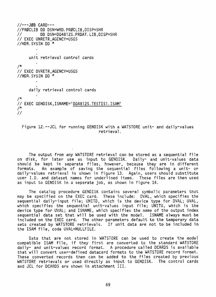
// J0B CARD //PR0CLIB DD DSN=WRD.PR0CLIB,DISP=SHR// DD DSN=DG4812S.PRDAT.LIB,DISP=SHR// EXEC UNRETR,AGENCY=USGS//HDR.SYSIN DD *
unit retrieval control cards
/*// EXEC DVRETR,AGENCY=USGS//HDR.SYSIN DD *
daily retrieval control cards
/*// EXEC GENDISK,ISNAME= I DG4812S.TESTIS1.I$AM I/*
Figure 12.--JCL for running GENDISK with a WATSTORE unit- and daily-valuesretrieval.
The output from any WATSTORE retrieval can be stored as a sequential file on disk, for later use as input to GENDISK. Daily- and unit-values data should be kept in separate files, however, because they are in different formats. An example of saving the sequential files following a unit- or daily-values retrieval is shown in figure 13. Again, users should substitute user I.D. and dataset names for underlined items. These files are then used as input to GENDISK in a separate job, as shown in figure 14.
The catalog procedure GENDISK contains several symbolic parameters thst may be specified on the EXEC card. These include: DVAL, which specifies the sequential daily-input file; UNITD, which is the device type for DVAL; UVAL, which specifies the sequential unit-values input file; UNITU, which is the device type for UVAL; and ISNAME, which specifies the name of the output index sequential data set that will be used with the model. ISNAME always must be included on the EXEC card. The other parameters default to the temporary data sets created by WATSTORE retrievals. If unit data are not to be included in the ISAM file, code UVAL=NULLFILE.
Data that are not stored in WATSTORE can be used to create the model compatible ISAM file, if they first are converted to the standard WATSTORE daily- and unit-values record format. A procedure called DCARDS is available that will convert user-defined datacard formats to the WATSTORE record format. These converted records then can be added to the files created by previous WATSTORE retrievals or used directly as input to GENDISK. The control cards and JCL for DCARDS are shown in attachment III.
69

// J0B CARD //PR0CLIB DD DSN=WRD.PR0CLIB,DISP=SHR // EXEC UNRETR,AGENCY=USGS //HDR.SYSIN DD *
unit retrieval control cards
/*//UNR.DATA0UT DD DSN=DG4812S.UVDATA.DATA,DI$P=(NEW,CATLG),// UNIT=0NLINE,SPACE=(TRK,(TO,5),RLSE)/*// EXEC DVRETR,AGENCY=USGS//HDR.SYSIN DD *
daily retrieval control cards
/*//DVR.BAKFILE DD D$N=DG4812$.DVDATA.DATA,DISP=(NEW,CATLG),// UNIT=0NLINE,SPACE=(TRK,(10,5),RLSE)/*
Figure 13.--JCL for saving unit- and daily-values sequential-output files.
// J0B CARD //PR0CLIB DD DSN=DG4812S.PRDAT.LIB,DISP=SHR// EXEC GENDI$K > DVAL='DG4812$.DVDATA.DATA I ,UNITD=0NLINE,// UVAL='DG4812S.UVDATA.DATA',UNITU=0NLINE,// I$NAME='DG4812S.TESTIS1. ISAM 1/*
Figure 14.--JCL for running GENDISK with previously stored online- sequential files.
70

Job Control Cards
The cataloged-procedure PRMODEL has been established on the U.S. Geologi cal Survey computer system. The JCL cards required to use the procedure are shown in figure 15. The name of the ISAM file created by GENDISK should be inserted, in single quotes, after INFILE=. The full procedure is listed in attachment I.
A number of input/output units are used in the procedure for data stor age, internal data management, and data-output files. An annotated list of these units and the file structure established on each is shown in table 7. With the exception of the files on units 2, 3, 20, and 21, all files have been established as temporary or permanent, and the deletion or retention of each has been predetermined. Files on unit 2 receive plot output for each HRU, and files on unit 3 receive daily data for each HRU. These files can be printed using the JCL shown in figure 16a. Unit 20 receives the predicted mean daily discharge file for permanent storage and further processing, when this option has been selected on card 1 of Card Group 1. A default Data Control Block (DCB) for a standard daily-values WATSTORE record has been established en the DO card for unit 20. However, a null Data Set Name (DSN) parameter has been included. A user DSN must be supplied when the output from a model run is to be saved. An example of how to insert the DSN parameter is shown in figure 16b. If the user selects the second data format option, the DCB parameters of Logical Record Length (LRECL) and Block Size (BLKSIZE) must be included with the DSN parameter on the override card shown in figure 16c. The LRECL parame ter should be set to 1480, and the BLKSIZE parameter should be set to 10360.
The predicted storm hydrograph may be saved as a permanent file on unit21 in the standard unit values format if this option has been selected on card1 of Card Group 1. A user DSN should be supplied, as shown in figure 16d.
// J0B CARD //PR0CLIB DO DSN=DG4812S.PRDAT.LIB,DISP=SHR // EXEC PRMQDEL,INFILE='DG4812S.TESTIS1.ISAM' //PR.SYSIN DD *
CARD GROUPS 1-8
/*//
Figure 15. OCL for using catalog-procedure PRMODEL.
71

Table
7.--
List
of
in
put/
outp
ut and
file
structures
IX)
1/0
unit
2 3 4 5 6 8 9 11 12 13 14 15 17 10 20 21 22 23 24 25 26 27 30
DISK(PLl)
SYSPRINT(PLI)
DSNAME
* A
___
___
&INV
&FHS
&DFHS
&UNI
TQ
&UNI
TP
&LA1IN
&SFILE
A A
___
___
___
___
A*
__
Unit
Line
printer
Line p
rinter
SYSD
KCA
RD INPUT
Line
printer
SYSD
KSY
SDK
SYSDK
SYSDK
SYSDK
SYSD
K
SYSDK
SYSDK
SYSDK
ONLI
NEON
LINE
CARD IN
PUT
CARD
INPUT
CARD
IN
PUT
CARD IN
PUT
CARD IN
PUT
CARD
INPUT
SYSDK
ONLI
NE
Line
printer
Spac
e
___
___
TRK(5,5)
___
---
TRK(
5,5)
128(1000)
TRK(lO.l)
TRK(5,1)
TRK(
10,5
)
TRK(
100,
5)
TRK(
100,
5)
5768(200)
TRK(100,5)
TRK(
5,5)
TRK(
5,5)
---
---
---
TRK(
5,15
)
CYL(
l)
-__
Disp
osit
ion
at j
ob en
d
___
DELETE ___
---
DELETE
DELETE
DELETE
DELETE
DELETE
DELETE
DELETE
DELETE
DELETE
NEW.CATLG
NEW.CATLG
___
---
---
---
DELETE
KEEP
_ _ _
RECF
M
--» ---
F VBS
VBS
VBS
VB VBS
F VBS
FB VB
---
FB VB
LRECL
___
___
___ ___
---
128
1472 656
108
5820
5820
___
5764
1656
1160
4
---
---
---
---
1480
1160
4
- -
BLKS
IZE
___
___
___
___
5896
6568
1088
5830
5830
5760
1200
0
1159
212
932
___
1036
0
1293
2
DSORG
Description
Outp
ut fi
le if daily
plot
s se
lect
ed.
Output f
ile
if pr
into
ut of individual HRU'S
sele
cted
.
Work
fil
e fo
r optimization.
Input
data
car
ds (c
ard
grou
p 1).
---
Line p
rinter o
utpu
t fr
om fo
rtra
n pr
ogra
ms.
---
Work fi
le fo
r sensitivity
anal
ysis
.DA
Dire
ct a
cces
s wo
rk fi
le fo
r op
timi
zati
on an-J
sens
itiv
ity
anal
ysis
.
Inve
ntor
y of un
it-v
alue
s ra
infa
ll da
ta by
water
year
.--
- Hydrograph separation in
form
atio
n fo
r each
stor
m period.
Hydrograph s
eparation
info
rmat
ion
for
each
unit-values
day.
Unit- values di
scha
rge
data
fo
r selected storm
periods.
---
Unit
-val
ues
rain
fall
da
ta fo
r ea
ch ra
in g
age
for
each
day
.DA
Dire
ct a
cces
s file to
st
ore
late
ral
and
upstream in
flow
to
chan
nel
segm
ents
.
Temp
orar
y file fo
r channel
segm
ent
stor
mhydrograph d
ata.
Output file t
o save p
redicted d
aily
di
scha
rge
---
Output f
ile
to save pr
edic
ted
unit d
isch
arge
.
-
Inpu
t da
ta c
ards
(c
ard
grou
p 2).
---
Input
data
car
ds (card
grou
p 3).
---
Input
data c
ards
(c
ard
grou
p 4)
.---
Input
data c
ards (c
ard
grou
p 5).
Input
data
car
ds (c
ard
grou
p 6).
Input
data
car
ds (c
ard
group
7,8).
Temp
orar
y fi
le fo
r predicted
and
obse
rved
dail
y di
scha
rge
data
.IS
Input
ISAM f
ile
containing d
aily
an
d unit
valu
es.
Line p
rint
er ou
tput
fr
om PL
1 pr
ogra
ms.
*Dummy fi
les
unless ov
erri
dden
in J
CL.
**As
sign
ed b
y us
er.

Figure 16a.
// J0B CARD //PR0CLIB DD DSN=DG4812S.PRDAT.LIB,DISP=SHR// EXEC PRM0DEL,INFILE='DG4812S.TESTIS1.ISAM I//PR.FT02F001 DD SYS0UT=A (include to print plots)//PR.FT03F001 DD SYS0UT=A (include if daily HRU data to be printed)//PR.SYSIN DD *
CARD GROUPS 1-8
/* //
Figure 16b.
// J0B CARD //PR0CLIB DD DSN=DG4812S.PRDAT.LIB,DISP=SHR// EXEC PRM0DEL,INFILE='DG4812S.TESTIS1.ISAM',// DV0UT='DG4812$.DVALUES.DATA'//PR. SYSIfTDCP*
CARD GROUPS 1-8
Figure 16.--JCL modifications to cataloged procedure PRMODEL. (a) Generateprinter plot and HRU output; (b) include Data Set Name (DSN) to storesimulated daily flows; (c) include DSN, Logical Record Length (LRECL)
and Block Size (BLKSIZE) to store simulated daily flows; and(d) include DSN to store simulated stormflows.
73

Figure 16c.
// J0B CARD //PR0CLIB DD DSN=DG4812S.PRDAT.LIB,DISP=SHR// EXEC PRM0DEL,DV0UT='DG4812S.DVALUES.DATA' i DVLREC=148Q > DVBLK=10360 t// INFILE=' DG4812S.TESTIS1 . ISAM'//PR.SYSIN DD~^
CARD GROUPS 1-8
/*
Figure 16d.
// J0B CARD //PR0CLIB DD DSN=DG4812S.PRDAT.LIB,DISP=SHR // EXEC PRM0DEL,UV0UT='DG4812S.l)VALUES.DATA' . // INFILE='DG4812S.TESTIS1.ISAM' //PR.SYSIN DD~*
CARD GROUPS 1-8
/*
Figure 16.--JCL modifications to cataloged procedure PRMQDEL (a) generateprinter plot and HRU output; (b) include Data Set Name (DSN) to storesimulated daily flows; (c) include DSN, Logical Record Length (LRECL)
and Block Size (BLKSIZE) to store simulated daily flows; and(d) include DSN to store simulated stormflows Continued.
74

The options selected in the system input stream will determine the number of files and input/output units that will be used in a particular model run. A daily-flow simulation requires fewer files than a daily and storm-event simulation. The number of files required will influence the core-storage requirements for model execution. The default REGION of 600 K should be sufficient for most model runs, but may need to be increased for a model run that includes optimization and storm simulation. This can be specified in the REGION parameter of the Execute (EXEC) card, as shown in figure 17. Param eters that may be specified on the EXEC card and their default values are listed in table 8.
System Input Cards
The PRMS input cards have been delineated into eight Card Groups. Card Group 1 is required for all model runs. The inclusion of one or more additional groups is a function of the options specified in Card Group 1. The Card Groups to be included in a data deck as a function of selected values for the variables IOPT, ISIM, ISEN, IPSW, and INPK are given in table 9.
Variable and parameter names and their definitions are given in all card groups. Additional information on most of these variables and parameters can be found in the Theoretical Development of System Library Components section. The subsections within the Theoretical Development section that provide this information are listed in brackets [] under the Definitions heading for each data card. When the subsection title appears with Card I.D., most or all items on that card are discussed in the referenced subsection. Variables and parameters that are self-explanatory have no subsection reference.
// J08 CARD /7PR0CLIB DD DSN=DG4812S.PRDAT.LIB,DISP=SHR// EXEC PRM0DEL,REGI0N.PR=750K,TIME.PR=5,INFILE='DG4812$.TESTIS1.ISAM'//PR.SYSIN DD *
CARD GROUPS 1-8
/*//
Figure 17. JCL for region and time modification to catalogedprocedure PRMODEL.
75
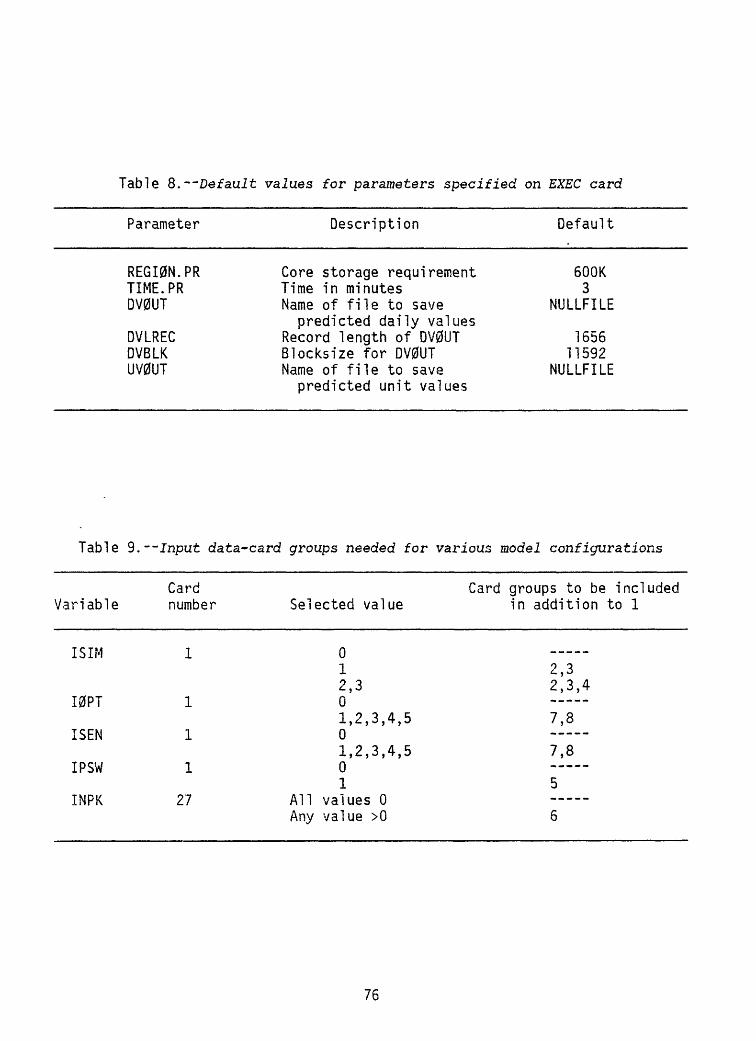
Table 8. Default values for parameters specified on EXEC card
Parameter
REGI0N.PRTIME. PRDV0UT
DVLRECDVBLKUV0UT
Description
Core storage requirementTime in minutesName of file to savepredicted daily values
Record length of DV0UTBlocksize for DV0UTName of file to savepredicted unit values
Default
500K3
NULLFILE
165611592
NULLFILE
Table 9. Input data-card groups needed for various model configuration
Variable
ISIM
I0PT
ISEN
IPSW
INPK
Card number
1
1
1
1
27
Selected value
01 2,3 01,2,3,4,5 01,2,3,4,5 01
All values 0Any value >0
Card groups to be included in addition to 1
_____2,3 2,3,4
7,8
7,8
5
6
76

Card Group 1: Parameter and Variable Initialization
This card group is read on input unit required for all simulation runs. Simulation and output options are established in this variables are initialized, and the physical hydrologic response units (HRU's) are established. //PR.SYSIN DD * card in the input card deck.
5 in subroutine DATIN and is options, types of input data, group. Model parameters and characteristics of the basin
Card group 1 follows a
CARD COLUMNS
1 1-915
FORMAT
'01SIM0PT 1 II
VARIABLES
ISIM
20 II I0BS
25 II I0PT
DEFINITIONS
Card I.D.Simulation mode switch
0=daily mode l=storm and daily mode 2=storm and daily modewith flow routing
3=storm and daily mode with flow and ,,sediment routing
Observed discharge data switch
0=no observed dischargedata
l=observed dischargedata input
Optimization mode switch [Optimization] O^no optimization l=daily optimization 2=daily optimizationwith correlationanalysis
3=optimization on stormvolumes
4=optimization on stormpeaks
5=optimization on stormpeaks and volumes
NOTE; IOPT is positive for Rosenbrock and negative for Gauss-Newton optimization.
77

CARD COLUMNS FORMAT VARIABLES DEFINITIONS
30
NOTE:
II ISEN Sensitivity analysis switch[Sensitivity Analysis]
0=no sensitivity analysis l=daily sensitivity analysis 2=daily sensitivity analysiswith correlation analysis
3=sensitivity analysis onstorm volumes
4=sensitivity analysis onstorm peaks
5=sensitivity analysis onstorm volumes and peakssimultaneously
An optimization and a sensitivity analysis cannot be run simultaneously. They can be run sequentially. See Card Group 8.
35 II ID0UT
40 II IU0UT
44-45
NOTE:
A2 SCODE
Store predicted daily mean stream- flow values switch 0=no storagel=store predicted and observed
daily values as sequential direct access data file by water year.Format is 370-word record with 4-word header and 366 data values.
2=Same as 1, except format is standard WATSTORE daily- values record.
Store predicted stormflow values switch0=no storagel=store predicted stormflow
values as sequential direct-access data file by storm. Format is standard WATSTORE unit- values record.
State code for daily- or unit- values output
ID0UT or IU0UT^O, output data set name must be included on //EXEC card.
78
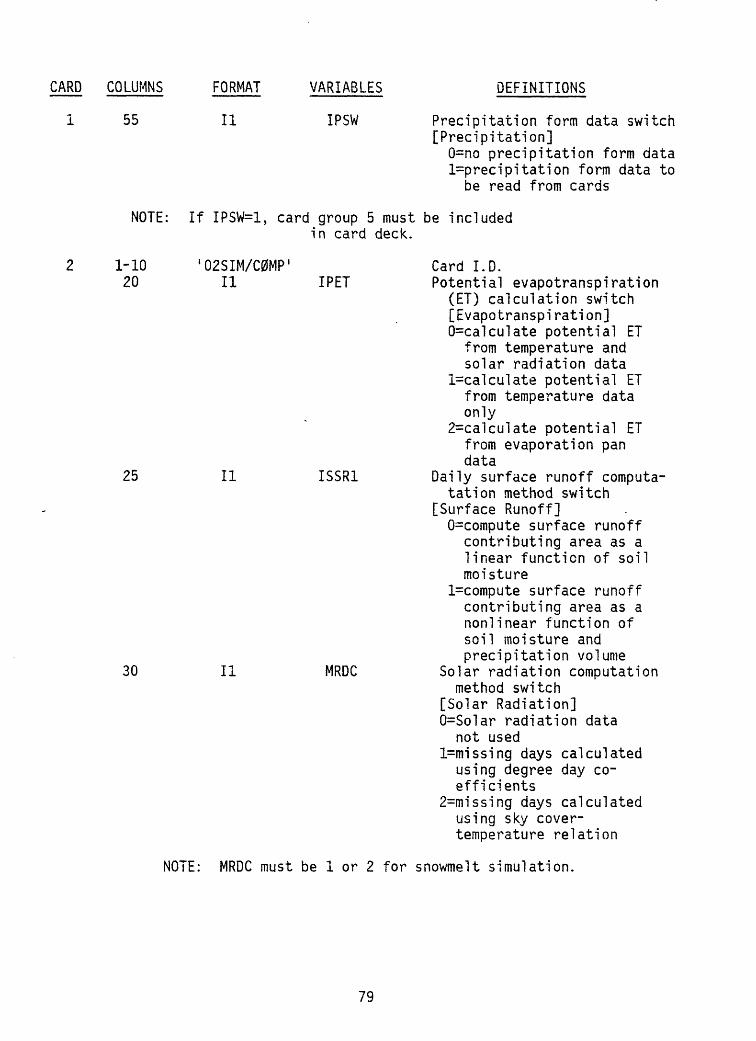
COLUMNS
55
NOTE:
FORMAT VARIABLES DEFINITIONS
II IPSW Precipitation form data switch[Precipitation]
0=no precipitation form data l=precipi tation form data to
be read from cards
If IPSW=1, card group 5 must be included in card deck.
1-10 20
02SIM/C0MP II IPET
25 II ISSR1
30 II MRDC
Card I.D.Potential evapotranspiration
(ET) calculation switch [Evapotranspiration] 0=calculate potential ET
from temperature and solar radiation data
l=calculate potential ET from temperature data only
2=calculate potential ET from evaporation pan data
Daily surface runoff computa-tation method switch
[Surface Runoff] 0=compute surface runoff
contributing area as a linear function of soil moisture
l=compute surface runoff contributing area as a nonlinear function of soil moisture and precipitation volume
Solar radiation computationmethod switch
[Solar Radiation] 0=Solar radiation data
not usedl=missing days calculated
using degree day co efficients
2=missing days calculated using sky cover- temperature relation
NOTE: MRDC must be 1 or 2 for snowmelt simulation.
79

CARD COLUMNS
2 35
FORMAT
1-6 11-80
1-7 11-15 16-20
21-25
'03TITL 1 17A4,A2
'04INIT1 11515
15
26-30
31-35
36-40
41-50
15
15
15
F10.0
1-7 11-15
16-20
21-25
26-30
31-35
36-40
'05INIT2' 15
15
15
15
15
15
VARIABLES DEFINITIONS
ISDN Switch for unit subsurface andground water flow routing
[Subsurface Flow, Ground Water] 0=surface runoff only
included in stormflow computation
l=surface, subsurface, and ground water included in stormflow computations
Card I.D.TITL Any title user wishes to print
as heading for all output
Card I.D.NDS Number of rain-gage data sets NRU Number of hydro!ogic response
units (HRU's) NRD Number of solar radiation
planes (one slope and aspect combination equals a plane). Equals all defined planes on basin plus 1 for horizontal surface
[Solar Radiation] NRES Number of subsurface flow routing
reservoirs [Subsurface Flow]
NGW Number of ground-water flowrouting reservoirs
[Ground Water] NST0R Number of surface-water detention
storage reservoirs [Reservoir Routing]
DAT Total basin drainage area, in acres
Card I.D. BYR Beginning year of data set
(for example, 1978) BM0 Beginning month of data set
(1-12) BDY Beginning day of data set
(1-31) EYR Ending year of data set
(for example, 1979) EM0 Ending month of data set
(1-12) EDY Ending day of data set
(1-31)
80

CARD COLUMNS FORMAT VARIABLES DEFINITIONS
8
1-9
11-15
16-20
1-10 11-15
'06MFS-MFN'
15 MFS
16-20
21-25
26-30
31-35
36-40
41-45
1-6 11-15
16-20
21-25 26-30 31-35 36-40 41-50
51-60
15 MFN
'07PRINT-0P' 15 IP0P1
15
15
15
15
15
15
'08PL0T' 15
15
15 15 15 15 F10.0
F10.0
IPUN3
IPUN4
IP0P2
IPUN1
IPUN2
1ST AT
IPL0T
IPLTYP
IMPLB IDPLB IMPLE IDPLE PLMX
PLMN
Card I.D.[Optimization]Beginning month of objective
function computation (dailyflow option)
Ending month of objectivefunction computation (dailyflow option)
Card I.D.Daily mean values print switch
0=print summary table1=0 plus annual summary2=1 plus monthly summary3=2 plus daily summary
Beginning month for printingdaily basin average values
Ending month for printingdaily basin average values
Individual HRU values print switch0=no printl=annual summary2=1 plus monthly summary3=2 plus daily summary
Julian date to start printingindividual HRU values
Julian date to stop printingindividual HRU values0=statistical summary not printed
l=statistical summary printed
Card I.D.Plot switch daily
0=no plot outputl=plot output
Plot type switch0=1inear scalel=semilog scale
Month plot begins (1-12) Day plot begins (1-31) Month plot ends (1-12) Day plot ends (1-31) The maximum plot value. For
semi log plots, this must bea power of 10 and equal 1,000 *PLMN
The minimum plot value. Forsemi log plots, this must bea power of 10 and non-zero
81

COLUMNS
16-65
FORMAT
'09DATATYPE 1 15
1015
10 1-6 11-60
'10PARM 1 1015
11 1-6
11-60
'11STAT 1
1015
12 1-8 (2 cards)
11-26,29-44, 47-62,65-80
'12STAIDC 1
4(2X,4A4)
VARIABLES DEFINITIONS
Card I.D. NDTY Number of data types being used
in the simulation IDUS(I) sSpecifies input data types. Ten
data types (I) in positionalorder are:
1) daily mean discharge2) daily pan evaporation3) daily maximum air tem
perature4) daily minimum air tem
perature5) daily solar radiation6) daily, user defined7) daily, user defined8) storm discharge9) daily precipitation
10) storm precipitation 0=data type not used l=data type used.
Card I.D.PARMCA(I) Parameter code (WATSTORE) used
with data types (I) specified in IDUS (positional using IDUS sequence, blank field if IDUS(I)=0).
See table 10.
Card I.D.
STATCA(I) Statistic code (WATSTORE) corres ponding to parameter codes on card 10 (positional using IDUS sequence, blank field if IDUS(I)=0). See table 10.
Card I.D.
STAIDC(I) Station I.D. for data types 1 through 8. D or U in first column of each field to indicate daily or unit station, respectively, plus station identification number which is either 15-digit latitude-longitude-sequence number, or 8-digit downstream order number, right- justified. Identification
82

Table 10.--Parameter codes and statistic codes used for inputdata types (IDUS)
Data type IDUS Parameter code Statistic code
Daily mean discharge Daily pan evaporation ------------Daily maximum air termperature
o c ... ..........op_ . ............
Daily minimum air temperature oc__._.________________...___op..........................
Daily solar radiation ------------Storm discharge -----------------Daily precipitation --------------Storm precipitation --------------
1 2 3
4
5 8 9 10
6050
2099998
2099998
30604545
36
11
226
1166
CARD COLUMNS
12
FORMAT VARIABLES
13 1-8 (NDS cards)
11-26,29-44
'13STAIDP
2(2X,4A4) STAIDP(I,J)
DEFINITIONS
number is left-justified when GENDISK was run using a standard WATSTORE retrieval, (positional using IDUS sequence, blank field if IDUS(I)=0)
Card I.D.
Station I.D. for precipitation data types 9 and 10. D or U in first column of each field to indicate daily or unit station, respectively, plus station identification number which is either 15-digit 1ati tude-1ongi tude-sequence number, or 8-digit downstream order number, right- justified. Identification number is left-justified when GENDISK was run using a standard WATSTORE retrieval.
One card required for each set of rain-gage data (I,J=1, NDS)
83

CARD COLUMNS FORMAT VARIABLES DEFINITIONS
14 1-4 (NRD cards) 5-6
10-13
20-25 26-30
31-35
NOTE:
15 1-5
11-70
16 1-5
11-70
17 1-9
11-15
'14RD'
12
A4
F5.2 F5.2
F5.2
Card I.D.[Solar Radiation]
I Index of this solar radiation plane, 1=1 is horizontal surface.
SA(I) Slope and aspect I.D. of this plane (for example, NW20 is northwest aspect, 20 percent slope)
SL Slope of plane (decimal ft/ft)ASP Aspect of plane (degrees clock
wise from north; for example, north=0.;E=90.0, and so forth)
ALAT Latitude of basin (degrees)
One no. 14 card is required for each solar radiation plane defined on the basin. The number of no. 14 cards is equal to NRD specified on card no. 4. The first card in this set is always the horizontal surface values. Not required if MRDC=0 and IPET=0 or 2. Required when MRDC > 0 or IPET=1.
'15RDM 1
12F5.2 RDM(I)
'16RDC'
12F5.2 RDC(I)
'17RAD-C0R'
F5.2 PARS
Card I.D.[Solar Radiation]MRDC=1Slope of maximum air tempera ture^) - degree day(y) relationship for months 1=1,12
MRDC=2Slope of max-min air
temperature(x) - sky cover(y) relationship for months 1=1,12
Card I.D.[Solar Radiation]
MRDC=1Y-intercept of maximum air
temperature(x) - degree day(y) relationship for months 1=1-12
MRDC=2Y-intercept of max-min air
temperature(x) - sky cover(y) relationship for months 1=1-12
Card I.D.[Solar Radiation]Predicted solar radiation correc
tion factor for summer day with precipitation
84
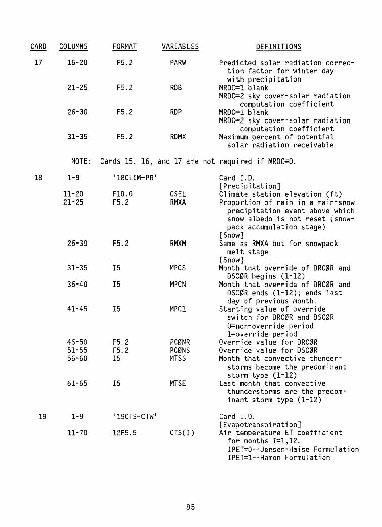
CARD COLUMNS
17
FORMAT
18
19
16-20
21-25
26-30
31-35
F5.2
F5.2
F5.2
F5.2
26-30
31-35
36-40
41-45
46-50 51-55 56-60
61-65
1-9
11-70
VARIABLES
PARW
RDB
RDP
RDMX
NOTE:
1-9
11-20 21-25
Cards 15, 16,
'18CLIM-PR 1
F10.0 F5.2
CSEL RMXA
F5.2
15
15
15
F5.2 F5.2 15
15
RMXM
MFCS
MPCN
MPC1
PC0NR PC0NS MTSS
MTSE
'19CTS-CTW'
12F5.5 CTS(I)
DEFINITIONS
Predicted solar radiation correc tion factor for winter day with precipitation
MRDC=1 blankMRDC=2 sky cover-solar radiation
computation coefficientMRDC=1 blankMRDC=2 sky cover-solar radiation
computation coefficientMaximum percent of potential
solar radiation receivable
Card I.D.[Precipitation]Climate station elevation (ft)Proportion of rain in a rain-snow precipitation event above which snow albedo is not reset (snow- pack accumulation stage)
[Snow]Same as RMXA but for snowpack melt stage
[Snow]Month that override of DRC0R and
DSC0R begins (1-12)Month that override of DRC0R and
DSC0R ends (1-12); ends last day of previous month.
Starting value of override switch for DRC0R and DSC0R 0=non-override period l=override period
Override value for DRC0ROverride value for DSC0RMonth that convective thunder
storms become the predominant storm type (1-12)
Last month that convective thunderstorms are the predom inant storm type (1-12)
Card I.D.[Evapotranspi rati on]Air temperature ET coefficient
for months 1=1,12. IPET=0 Jensen-Haise Formulation IPET=1 Hamon Formulation
85

CARD COLUMNS FORMAT VARIABLES DEFINITIONS
19 71-75 F5.2 CTW
20 1-5 11-70
21
22
23
24
25
1-6
11-70
1-5
11-70
1-5
11-70
1-5
11-70
1-9
11-15
16-20
21-25
26-30
31-35
36-40
20PAT' 12F5.2
'21AJMX 1
12F5.2
'22TLX'
12F5.2
'23TLN 1
12F5.2
'24EVC 1
12F5.2
F5.2
F5.2
PAT(J)
AJMX(J)
TLX(I)
TLN(I)
EVC(I)
'25SN0-VAR'
15 ISP1
15 ISP2
F5.2 EAIR
F5.2 FWCAP
DENI
DENMX
Proportion of potential evapo- transpiration that is subli mated from a snow surface (decimal form)
[Snow]
Card I.D.Maximum air temperature, which
when exceeded forces precipi tation to be rain regardless of minimum air temperature, for months J=l,12
Card I.D.[Precipitation]Adjustment proportion of rain in
a rain-snow mix event, for monthsJ=l,12
Card I.D. [Temperature]Lapse rate for maximum daily air temperature for months 1=1,12
Card I.D. [Temperature]Lapse rate for minimum daily air temperature for months 1=1,12
Card I.D.[Evapotranspiration] Evaporation pan coefficient for
months 1=1,12
Card I.D.[Snow]Julian date to start looking for
spring snowmelt stage Julian date to force snowpack to
spring snowmelt stage Emissivity of air on dayswithout precipitation
Free water-holding capacity ofsnowpack expressed as decimalfraction of total snowpackwater equivalent
Initial density of new-fallensnow (gm/cm3 )
Average maximum snowpack density(gm/cm3 )
86

CARD COLUMNS FORMAT VARIABLES
25
26
27
28
29
30
31
41-45
46-50
1-5
11-70
1-7
11-80
1-5
11-80
1-4
11-80
1-6
11-80
1-10
11-15 21-25 31-35,etc.
16-20 26-30 36-40,etc.
F5.2 SETC0N
F5.0 BST
'26CEN'
12F5.0 CECN(I)
'27PKADJ'
1415 INPK(I)
'28RES 1
14F5.2
'29GW
14F5.2
RES(I)
GW(I)
'30KRSP'
1415 KRSP(I)
'31RESMX-EX 1
F5.2 RESMX(I)
F5.2 REXP(I)
DEFINITIONS
Snowpack settlement time constant
Temperature above which precipi tation is all rain and below which it is all snow
[Precipitation]Card I. D.[Snow]Convecti on-condensati on energy
coefficient for months 1-1,12(cal/°C above zero)
Card I.D.[Precipitation]Julian dates for adjusting
computed snowpack water equivalents from snowcourse data. One date for each water-year run. Use zero for years without an update. For each water year with a nonzero value, one Group 6 data card is required.
Card I.D. [Sursurface Flow] Storage in each subsurface flow
routing reservoir (in.)Card I.D. [Ground Water]Storage in each ground-water
flow routing reservoir (in.)
Card I.D.[Ground Water]The index of the ground-water
reservoir receiving recharge from subsurface reservoir I; 1=1, NRES
Card I.D.[Ground Water]Coefficient for computing
recharge from subsurface reservoir I to its designated ground-water reservoir
Exponent coefficient for computing recharge from sub surface reservoir I to its designated ground-water reservoir
87

CARD COLUMNS FORMAT VARIABLES DEFINITIONS
32
33
34
35
36
1-6
11-80
1-6
11-80
1-5
11-80
NOTE:
1-5 9-10
11-13
14-18 19-25
26-30
31-35
36-40
'32RSEP 1
14F5.2 RSEP(I)
'33GSNK 1
14F5.2 GSNK(I)
'34RCB 1
14F5.2 RCB(I)
1-9
11-20,31-40,51-6021-30,41-50,61-70
'35RCF-RCP'
F10.0
F10.0
RCF(n
RCP(I)
Card I.D.[Ground Water]Coefficient used in computing
recharge rate from subsurface reservoir I to its designated ground-water reservoir
Card I.D.[Ground Water]Coefficient used in computing the
recharge rate from ground-water reservoir I to a ground-water sink
Card I.D.[Ground Water]Ground-water routing coefficient
for each ground-waterreservoir I
Card I.D.[Subsurface Flow]Subsurface flow routing coeffi
cient for each subsurface reservoir I
Subsurface flow routing coeffi cient for each subsurface reservoir I
One set of cards, 36 through 38, is required for each HRU (NRU on card 3).
'36RU1 11213
F5.0 F7.0
15
IRU IRD
SLP ELV
IC0V
F5.2
F5.2
C0VDNS
C0VDNW
Card I.D.HRU I.D.Solar radiation plane index
associated with this HRU Slope (decimal form) Mean elevation of HRU (feet above
MSL)Predominant vegetation cover
type, 0=bare l=grasses 2=shrubs 3=trees
Summer vegetation cover density(decimal)
Winter vegetation cover density (decimal)
88

CARD COLUMNS FORMAT VARIABLES DEFINITIONS
36 41-45 F5.2
46-50
51-55
56-60
61-62
63-64
65
F5.2
F5.2-
F5.2
12
12
11
66-70
37
71-75
76-80
1-5 9-10
11-15
16-20
F5.2
F5.2
F5.2
'37RU2 11215
F5.2
TRNCF Transmission coefficient for short-wave radiation through the winter vegetation canopy (decimal form)
[Snow]SNST Interception storage capacity of
major winter vegetation for snow (inches water equivalent)
RNSTS Summer rain interception storage capacity of major vegetation (in.)
RNSTW Winter rain interception storage capacity of major vegetation (in.)
ITST Month to look for start of tran spiration (1-12)
[Evapotranspiration] ITND Month transpiration ends (1-12);
ends last day of previous month [Evapotranspiration]
ITSW Starting value for transpiration switch0=vegetation dormant l=vegetation transpiring
[Evapotranspiration] CTX Air temperature coefficient for
evapotranspi rati on computati ons [Evapotranspi ration]
IPET=0 Jensen-HaiseFormulation
IPET=1 Blank IPET=2 Blank
TXAJ Adjustment for maximum airtemperature for slope and aspect
[Temperature] TNAJ Adjustment for minimum air
temperature for slope and aspect [Temperature]
Card I.D.IRU HRU I.D. IS0IL Soil type,
l=sand,2=1oam,3=clay
SMAX Maximum available water-holdingcapacity of soil profile (0.3 -15 bars) (in.)
[Soil Moisture]
89

CARD COLUMNS FORMAT VARIABLES DEFINITIONS
37 21-25 F5.2
26-30 F5.2
31-35 F5.2
36-40 F5.2
41-45
46-50
51-55
56-60
61-65
66-70
71-73
74-76
F5.2
F5.2
F5.2
F5.2
F5.2
F5.2
13
13
SMAV Current available water in soilprofile (in.)
[Soil Moisture]REMX Maximum available water-holding
capacity of soil recharge zone (0.3 - 15 bars) (in.)
[Soil Moisture] RECHR Current available water-holding
capacity of recharge zone (in.) [Soil Moisture]
SRX Maximum daily snowmelt infiltra tion capacity of soil profile (in.) when profile is at field capacity
[Soil Moisture]SCX Maximum possible contributing area
as proportion of total HRU area (decimal form)
[Surface Runoff]SCN ISSR1=0 Minimum possible contrib
uting area as proportion of total HRU area (decimal form)
[Surface Runoff]ISSR1=1 Coefficient in contribut
ing area moisture index rela tionship
[Surface Runoff] SCI ISSR1=0 blank
ISSR1=1 Coefficient in contribut ing area moisture index relation ship
[Surface Runoff]IMPERV Effective impervious area as
proportion of total HRU (decimal form)
[Surface Runoff] RETIP Maximum retention storage on
impervious area (in.) [Surface Runoff]
SEP Maximum daily recharge from soil moisture excess to designated ground-water reservoir (KGW), (in./d)
KRES Index of subsurface reservoir receiving recharge from HRU
[Subsurface Flow]KGW Index of ground-water reservoir
receiving recharge from HRU
90

CARD COLUMNS FORMAT VARIABLES DEFINITIONS
37 77-79 13
38
39
1-5
26-30
31-35
36-40
21-25
26-30
31-35
36-40
41-50
51-60
61-70 71-80
38RU3 1
9-1011-1314-2021-25
1213F7.0F5.2
IRUKDSDARUUPC0R
F5.2
F5.2
F5.2
1-6
11-15
16-20
'39ST0R 1
15
15
KST0R
IRTYP
15
15
15
15
F10.2
F10.2
F10.2 F10.2
KST0R Index of surface-water detention storage reservoir receiving runoff from HRU
[Reservoir Routing]
Card I.D. [Precipitation] HRU I.D.Index of rain gage Drainage area for HRU (acres) Rain correction for storm precipi tation for rain gage KDS
DRC0R Rain correction for dailyprecipitation for rain gageKDS
DSC0R Snow correction for dailyprecipitation for rain gageKDS
TST Temperature index to determinespecific date of start oftranspiration
Card I.D.[Reservoir Routing]Index of surface water storagereservoir
Type of reservoir routing 8=Puls routing 9=Linear routing
NS0S IRTYP=8 The number of outflow- storage data pairs to be input (maximum of 10)
IRTYP=9 blankIRUP1 Index (KST0R) of upstream surface-
water storage reservoir 1, else blank
IRUP2 Index (KST0R) of upstream surface- water storage reservoir 2, else blank
IRUP3 Index (KST0R) of upstream surface- water storage reservoir 3, else blank
RCS IRTYP=8 blankIRTYP=9 routing coefficient
ST0 Initial reservoir storage(cfs-days)
QR0 Initial day mean outflow (cfs) DIN1 Initial day mean inflow (cfs)
91
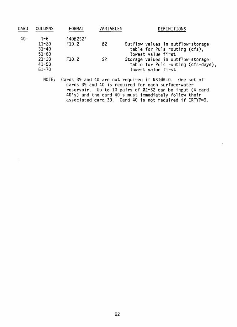
CARD COLUMNS FORMAT VARIABLES DEFINITIONS
40 1-6 '4002S2'11-20 F10.2 02 Outflow values in outflow-storage31-40 table for Puls routing (cfs),51-60 lowest value first21-30 F10.2 S2 Storage values in outflow-storage41-50 table for Puls routing (cfs-days),61-70 lowest value first
NOTE: Cards 39 and 40 are not required if NST0R=0. One set of cards 39 and 40 is required for each surface-water reservoir. Up to 10 pairs of 02-S2 can be input (4 card 40 ! s) and the card 40's must immediately follow their associated card 39. Card 40 is not required if IRTYP=9.
92

Card Group 2: Storm Period Selection
This card group is read on input unit 22 in subroutine INVIN and is required only when the ISIM variable (Card Group 1, card 1) is greater than zero. These data define the storm periods to be simulated in a storm mode and the options for storm peak and volume computations. A storm period is defined as one or more consecutive days of storm rainfall. Each storm-period selec tion card set also describes the number of stormflow hydrograph segments within the storm period. A hypothetical storm period containing two hydrograph segments is shown in figure 18. If storm-mode subsurface and groun'd-water flow routing are selected (ISUN=1), storm computations are made on full-day time intervals, and hydrograph segmentation is not required. Card group 2 follows a //SYSIN2 DD * card in the input deck.
Qo oLU COocLU CL
LU LU U-
O 00
O
LU
8<
OC/5
I I I I M I i 1 I
Segment 2
1200 May 3, 1978
1200 May 4, 1978
1200 May 5. 1978
1200 May 6. 1978
TIME
Figure 18.--Delineation of hydrograph segments within a storm period,
93
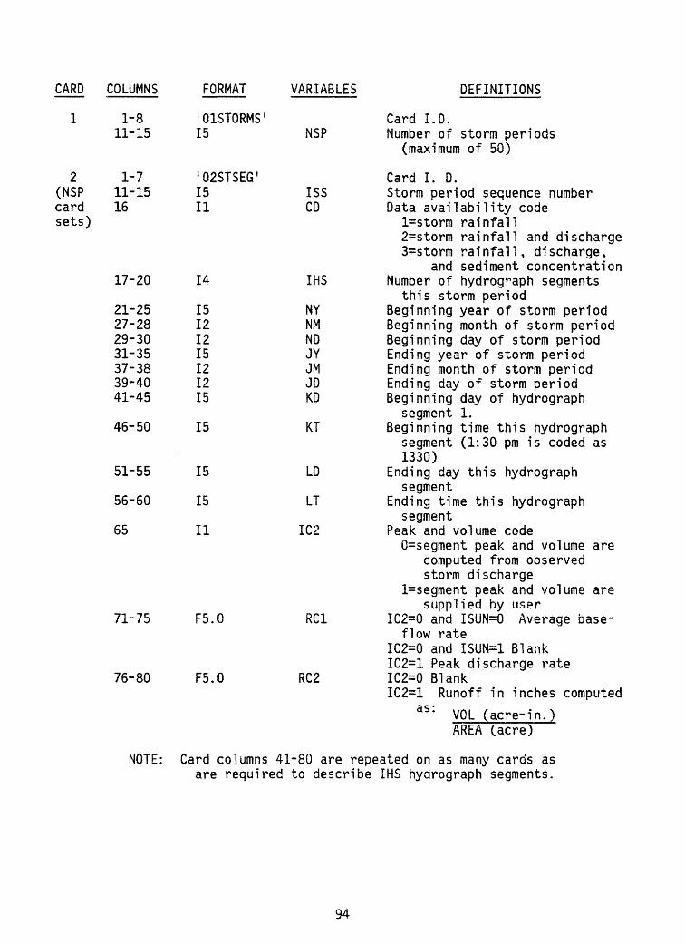
CARD COLUMNS
1 1-8 11-15
2(NSP card sets)
1-7 11-15 16
17-20
21-25 27-28 29-30 31-35 37-38 39-40 41-45
46-50
51-55
56-60
65
71-75
76-80
FORMAT
'01STORMS 1 15
'02STSEG15II
14
15121215121215
15
15
15
II
F5.0
F5.0
VARIABLES
NSP
ISS CD
IHS
NY NM ND JY JM JD KD
KT
LD
LT
IC2
RC1
RC2
DEFINITIONS
Card I.D.Number of storm periods
(maximum of 50)
Card I. D.Storm period sequence numberData availability code
l=storm rainfall2=storm rainfall and discharge3=storm rainfall, discharge,
and sediment concentration Number of hydrograph segments
this storm period Beginning year of storm period Beginning month of storm period Beginning day of storm period Ending year of storm period Ending month of storm period Ending day of storm period Beginning day of hydrograph
segment 1. Beginning time this hydrograph
segment (1:30 pm is coded as1330)
Ending day this hydrographsegment
Ending time this hydrographsegment
Peak and volume code0=segment peak and volume are
computed from observed storm discharge
l=segment peak and volume aresupplied by user
IC2=0 and ISUN=0 Average base-flow rate
IC2=0 and ISUN=1 Blank IC2=1 Peak discharge rate IC2=0 Blank IC2=1 Runoff in inches computed
(acre-in.)
NOTE
AREA (acre)
Card columns 41-80 are repeated on as many cards as are required to describe IHS hydrograph segments.
94

Card Group 3: Infiltration/Upland Erosion Parameters
This card group is read on input unit 23 in subroutine INVIN and is required when the variable ISIM (Card Group 1, card 1) is greater than zero. It defines the infiltration and erosion characteristics of an HRU for storm- mode computations. The parameters KSAT, PSP, RGF, and DRN are always included on the card. However, the remaining parameters are only required if ISIM equals 3. One card is required for each HRU defined. Card group 3 follows a //SYSIN3 DD * card in the input card deck.
CARD COLUMNS
1 1-7 (NRU cards)
8-10 11-15
16-20
21-25
26-30
31-40
41-50
51-60
61-70
71-80
FORMAT
01IN-ER 1
13 F5.0
F5.0
F5.0
F5.0
F10.0
F10.0
F10.0
F10.0
F10.0
VARIABLES
IRU KSAT
PSP
RGF
DRN
KR*
HC*
KF*
KM*
EN*
DEFINITIONS
Card I.D.[Infiltration, Sediment]HRU I.D.Hydraulic conductivity of trans mission zone (inches per hour)
The product of moisture defi cit and capillary drive for RECHR equal to field capacity, REMX (in.)
Ratio of PSP at field capacity (RECHR=REMX) to PSP at wilting point (RECHR=0)
Drainage factor for redistribu tion of saturated moisture storage, SMS, to recharge zone moisture storage, RECHR, as a fraction of hydraulic conduc tivity, KSAT
Parametric coefficient in rain drop-flow depth soil detach ment relation
Parametric coefficient in raindrop-flow depth soil detachment relation
Parametric coefficient in runoff detachment relation
Parametric coefficient in sediment transport capacity relation
Parametric coefficient in sediment transport capacity relation
*NOTE: Required only if ISIM=3.
95

Card Group 4: Flow and Sediment Routing Specifications
This card group is read on input unit 24 in subroutine INVIN and is required only if the variable ISIM (Card Group 1, card 1) is equal to 2 or 3. These cards define the type and flow characteristics of the overland flow planes and channel, reservoir, and junction segments into which the basin has been divided. One card 2 is required for each overland flow plane defined and one card 4 is required for each channel, reservoir, and junction segment defined. Card group 4 follows a //SYSIN4 DD * card in the input card deck.
An example watershed with three HRU's is shown in figure 19a. HRU 1 is the headwater area of the watershed, HRU 2 is the area adjacent to the main channel and major tributaries, and HRU 3 is an area adjacent to the main channel in the lower part of the watershed. A schematic diagram delineating the segmentation of the figure 19a sample watershed into nine overland-flow planes and nine channel segments is shown in figure 19b. It should be noted that overland-flow planes delineated within an HRU and having the same length, slope, and roughness characteristics can be assigned the same plane identifi cation (PCRID). All the overland-flow planes defined except 0F8 have each been used at least twice in their respective HRU's. Flow-plane characteris tics are described on card 2 of this group and one card is completed for each overland-flow plane defined. There is no sequential order required for card 2's. The model computes the rainfall excess and overland-flow hydrograph for a unit width on each defined flow plane. This information then is stored and reused each time a given flow plane is specified as lateral inflow to a channel segment.
Channel segments also can be reused when two or more channel segments have the same length, lateral inflows, and upstream inflows. The outflow hydrograph for the channel segment will be computed once and reused as many times as specified. In figure 19b, channel segments Cl, C2, and C6 each are used at least twice. Reuse of overland-flow plane and channel segments where possible decreases storm-mode computation time by eliminating repetitive computations for similar areas. However, areas reused must be within the same HRU to ensure use of the same antecedent soil-moisture conditions and storm-precipitation record.
The channel segments from figure 19b and the upstream and lateral inflows to each are listed in table 11. This information is placed on card 4 of this group and one card 4 for each channel segment is required. Table 11 is presented to illustrate the two card-sequencing requirements for card 4's. The first is that for any channel to be used as an upstream inflow, it must be defined in the channel segment sequence prior to its use. The second require ment is specified for efficient processing and storage. It states that when a channel segment uses as an upstream inflow the channel segment defined by the previous card 4, this previous card 4 segment must appear as upstream inflow 1 (UP1). For example, in table 11, channel segment C2 must appear as Upstream 1 inflow for channel segment C3. This eliminates the need to store and retrieve this segment information before it is processed.
96

EXPLANATION
Hydro log i c- respon se unit (HWJ) boundary
Flow-plane boundary
Channel network
B
EXPLANATION
iinB Hydro logic-response unit (HRU) boundary
C1 Channel segment and number
j QF3 j Flow plane and number
Figure 19. Delineation of sample watershed: (A) Hydrologic response unit (HRU), flow-plane boundaries, and channel network;
(B) schematic of flow planes and channel segments.
97
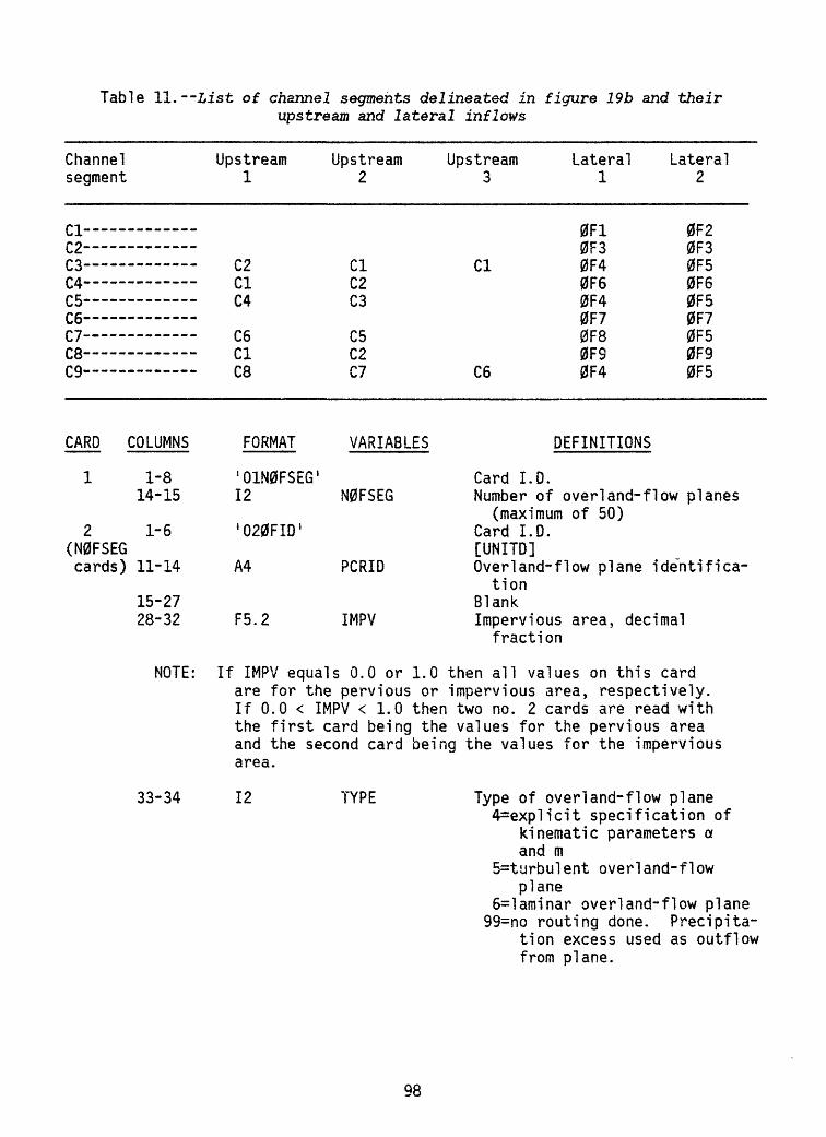
Table 11. List of channel segments delineated in figure 19b and theirupstream and lateral inflows
Channel segment
C2 w£.
ro --------uoPA - , _Vrf"T/> r _____ _ _______LO-- -
t,o ------- C7 t> /uo -----------^y-- -----------
CARD COLUMNS
1 1-8 14-15
Upstream 1
C2 Cl C4
C6 Cl C8
FORMAT
'01N0FSEG' 12
Upstream 2
Cl C2 C3
C5 C2 C7
VARIABLES
N0FSEG
Upstream 3
Cl
C6
Card I. Number
Lateral 1
0F1 0F3 0F4 0F6 0F4 0F7 0F8 0FS 0F4
DEFINITIONS
Lateral 2
0F2 0F3 0F5 0F6 0F5 0F7 0F5 0F9 0F5
D. of overland-flow planes
2 1-6 (N0FSEG cards) 11-14
15-27 28-32
NOTE:
33-34
'020FID'
A4 PCRID
F5.2 IMPV
(maximum of 50)Card I.D.[UNITD]Overland-flow plane identifica
tionBlankImpervious area, decimal
fraction
If IMPV equals 0.0 or 1.0 then all values on this card are for the pervious or impervious area, respectively. If 0.0 < IMPV < 1.0 then two no. 2 cards are read with the first card being the values for the pervious area and the second card being the values for the impervious area.
12 TYPE Type of overland-flow plane 4=explicit specification of
kinematic parameters a and m
5=turbulent overland-flowplane
6=laminar overland-flow plane 99=no routing done. Precipita
tion excess used as outflow from plane.
98
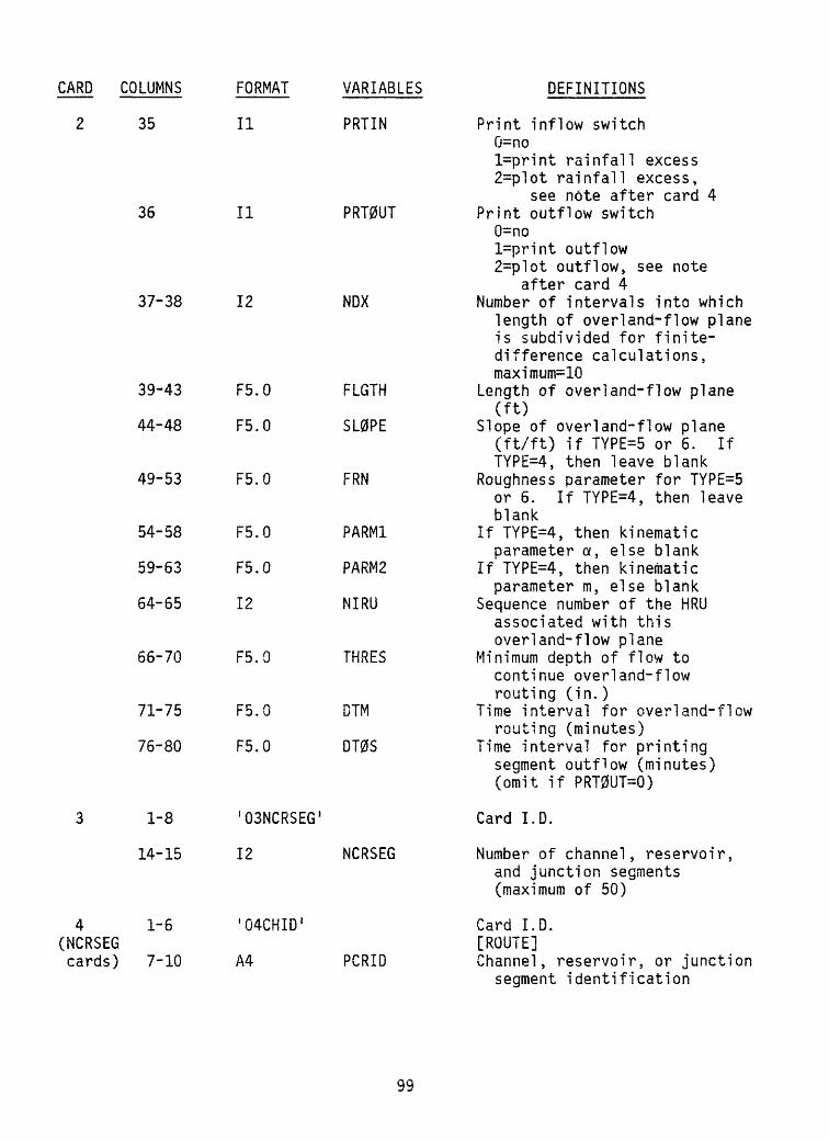
CARD COLUMNS FORMAT VARIABLES DEFINITIONS
35 II PRTIN
36
37-38
39-43
44-48
49-53
54-58
59-63
64-65
66-70
71-75
76-80
1-8
14-15
4 1-6 (NCRSEG cards) 7-10
II
12
F5.0
F5.0
F5.0
F5.0
F5.0
12
F5.0
F5.0
F5.0
PRT0UT
NDX
FLGTH
SL0PE
FRN
PARM1
PARM2
NIRU
THRES
DTM
DT0S
'03NCRSEG 1
12 NCRSEG
'04CHID 1
A4 PCRID
Print inflow switch0=nol=print rainfall excess2=plot rainfall excess,
see n6te after card 4 Print outflow switch
0=nol=print outflow2=plot outflow, see note
after card 4 Number of intervals into which
length of overland-flow planeis subdivided for finite- difference calculations,maximufiFlO
Length of overland-flow plane(ft)
Slope of overland-flow plane(ft/ft) if TYPE=5 or 6. IfTYPE=4, then leave blank
Roughness parameter for TYPE=5or 6. If TYPE=4, then leaveblank
If TYPE=4, then kinematicparameter a, else blank
If TYPE=4, then kinematicparameter m, else blank
Sequence number of the HRUassociated with thisoverland-flow plane
Minimum depth of flow tocontinue overland-flowrouting (in.)
Time interval for overland-flowrouting (minutes)
Time interval for printingsegment outflow (minutes)(omit if PRT0UT=Q)
Card I.D.
Number of channel, reservoir, and junction segments (maximum of 50)
Card I.D. [ROUTE]Channel, reservoir, or junction
segment identification
99

CARD COLUMNS FORMAT
4 11-14 A4
VARIABLES
UP1
15-18
19-22
23-26
A4
A4
A4
UP2
UP3
RBC
27-30 A4 LBC
33-34 12 TYPE
35 II PRTIN
36 II PRT0UT
37-38 12 NDX
DEFINITIONS
Identification of upstream inflow segment number 1, else blank if none. If immedi ately preceding channel seg ment (PCRID) is used as up stream inflow, it must be designated as DPI.
Identification of upstream inflow segment number 2, else blank if none.
Identification of upstream inflow segment number 3, else blank if none
Identification of overland-flow plane that contributes lateral inflow to right side of channel, else blank if none
Identification of overland-flow plane that contributes lateral inflow to left side of channel, else blank if none
Type of segmentl=rectangular open channel 3=triangular open channel 4=explicit specification of
kinematic parameters a and m
7=junction8=reservoirs, Puls routing 9=reservoir, linear routing
Print/plot inflow switch0=nol=print inflow to segment2=plot inflow to segment,
see note Print/plot outflow switch
0=nol=print outflow from segment2=plot outflow from segment,
see note If TYPE < 7 Number of intervals into which
the length of channel segment
100

CARD COLUMNS FORMAT VARIABLES DEFINITIONS
39-43
44-48
49-53
54-58
59-63
66-70
71-75
76-80
F5.0
F5.0
F5.0
F5.0
F5.0
F5.0
F5.0
F5.0
FLGTH
SL0PE
FRN
PARM1
PARM2
THRES
DTM
DT0S
is to be subdivided for finite-difference computa tions, maximum=10
If TYPE=8, number of outflow- storage pairs in Puls routing table
If TYPE=9, blankLength of channel segment in
feetSlope of channel segment
(ft/ft), not required if TYPE=4, 7, 8, or 9
Roughness (Manning's "n") of channel segment, not required if TYPE=4, 7, 8, or 9
If TYPE=1, the width of channel (ft)
If TYPE=3, then ratio of hori zontal to vertical change in side slope (right side)
If TYPE=4, then kinematic parameter a
Else leave blankIf TYPE=3, same as TYPE 3 above
(left side)If TYPE=4, then kinematic parameter m,
Else leave blankMinimum rate of discharge to
continue channel flow routing (cfs)
Time interval for channel flow routing (minutes)
If ITYPE=8 must be 5 or 15 minutes
Time interval for printing segment outflow (minutes) (omit if PRT0UT=0)
Note: Stormflow plots for up to 8 overland-flow planes and/or channel segments may be requested.
Card Group 5: Precipitation Form Adjustment
This card group is read on input unit 25 in subroutine TIMEY and is required only if the variable IPSW (Card Group 1, card 1) is equal to 1. A set of cards 1 and 2 are required for each water year in a simulation run. Precipitation occurring on the Julian dates specified will be considered all snow or all rain, thus overriding the algorithm in subroutine PRECIP which apportions snow and rain on the basis of air temperature. These cards
101

normally are used when continuous records of precipitation and air temperature are available to delineate precipitation form. The cards are read on the first day of each water year. Card group 5 follows a //SYSIN5 DO * card in the input card deck.
CARD COLUMNS
1 1-6
11-15
16-80
11-80
1-6
11-15
16-80
FORMAT
'01SPFS'
15
1315
VARIABLES
Kl
KSV
1415
'02SPFR 1
15
1315
KSV
K2
KSV
11-80 1415 KSV
DEFINITIONS
Card I.D.[PRECIP]Number of dates to be read
(at least 1)Julian dates of days with
precipitation events whose form should be considered all snow. Zero for the first date indicates no snow form changes
Continuation cards if more than 13 values are used
Card I.D. [PRECIP]
Number of dates to be read (at least 1)
Julian dates of days with precipitation events whose form should be considered all rain. Zero for the first date indicates no rain form changes
Continuation cards if more than 13 values are used
Card Group 6: Snowpack Adjustment
This card group is read on input unit 26 in subroutine TIMEY and is required only when the array INPK (Card Group 1, card 27) has a nonzero value in the array element associated with the current water year. INPK is an array containing one Julian date for each water year when snowcourse data are to be input to update snowpack water equivalent values computed by the model. The data from this card group are used to adjust the snowpack water equivalents on each hydrologic response unit. These cards are read on the first day of each water year. Card group 6 follows a //FT26F001 DD * in the input card deck.
102
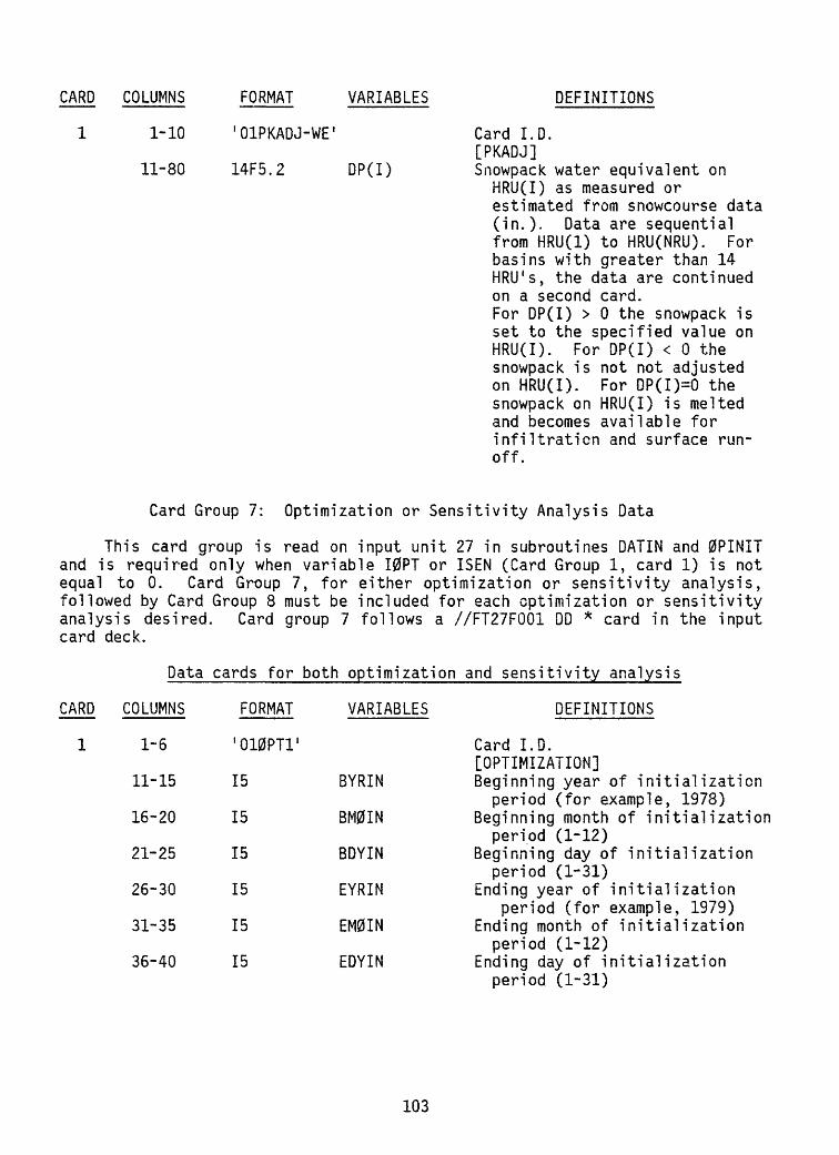
CARD COLUMNS FORMAT VARIABLES DEFINITIONS
1 1-10
11-80
01PKADJ-WE'
14F5.2 DP(I)
Card I.D.[PKADJ]Snowpack water equivalent on
HRU(I) as measured or estimated from snowcourse data (in.)- Data are sequential from HRU(l) to HRU(NRU). For basins with greater than 14 HRU's, the data are continued on a second card. For DP(I) > 0 the snowpack is set to the specified value on HRU(I). For DP(I) < 0 the snowpack is not not adjusted on HRU(I). For DP(I)=0 the snowpack on HRU(I) is melted and becomes available for infiltration and surface run off.
Card Group 7: Optimization or Sensitivity Analysis Data
This card group is read on input unit 27 in subroutines DATIN and 0PINIT and is required only when variable I0PT or ISEN (Card Group 1, card 1) is not equal to 0. Card Group 7, for either optimization or sensitivity analysis, followed by Card Group 8 must be included for each optimization or sensitivity analysis desired. Card group 7 follows a //FT27F001 DD * card in the input card deck.
Data cards for both optimization and sensitivity analysis
CARD COLUMNS
1 1-6
11-15
16-20
21-25
26-30
31-35
36-40
FORMAT VARIABLES DEFINITIONS
'010PT1 1 Card I.D.[OPTIMIZATION]
15 BYRIN Beginning year of initializationperiod (for example, 1978)
15 BM0IN Beginning month of initializationperiod (1-12)
15 BDYIN Beginning day of initializationperiod (1-31)
15 EYRIN Ending year of initializationperiod (for example, 1979)
15 EM0IN Ending month of initializationperiod (1-12)
15 EDYIN Ending day of initializationperiod (1-31)
103

'020PT2'
15 BYR0P
COLUMNS FORMAT VARIABLES DEFINITIONS
Card I.D. [OPTIMIZATION]Beginning year of optimization
or sensitivity analysis period (for example, 1979)
15 BM00P Beginning month of optimizationor sensitivity analysis period (1-12)
15 BDY0P Beginning day of optimization orsensitivity analysis period (1-31)
15 EYR0P Ending year of optimization orsensitivity analysis period (for example, 1980)
15 EM00P Ending month of optimization orsensitivity analysis period(1-12)
15 EDY0P Ending day of optimization orsensitivity analysis period(1-31)
'03I0BF' Card I.D.[OPTIMIZATION]
15 I0BF * Objective function selectionswi tenl=sum of absolute values of
the differences between predicted and observed flows
2=sum of squares of dif ferences between predicted and observed flows
15 ITRANS Logarithmic transformationswi tch0=do not transform predicted and observed runoff values before objective function computa tion
l=transform predicted and observed runoff values before objective function computation
NOTE: If this is a sensitivity analysis run, skip to the"Data cards for sensitivity analysis" section for card 4.
16-20
21-25
26-30
31-35
36-40
1-6
11-15
16-20
104

Data cards for optimization
These data cards define which model parameters are to be optimized in a given run and the boundary constraints on each parameter. The storm periods for optimizing unit storm parameters are also specified here.
CARD COLUMNS
4 1-6
11-15
16-20 21-25
NOTE:
1-8
11-15
16-20
FORMAT VARIABLES DEFINITIONS
'040PT4 1 Card I.D.[OPTIMIZATION]
15 NV Number of parameters to beoptimized
15 NTRY Number of optimization cycles15 IPRI0R Prior information switch
0=no normal prior information l=normal prior information
One set of cards 5 and 6 is required for each parameter to be optimized (NV on card 4).
'05PARAM1 1
15 L0P
15 IL0PL
21-25 15 NVAR
26-30 IDSW
31-35 F5.2
Card I.D.[OPTIMIZATION]Parameter to be optimized. See
table 3 for parameter numbersSwitch indicating whether each
value of a distributed parameter is to be adjusted by the same magnitude or same
. percentage of the initial value0=same magnitude l=same percentage of initial
valueNumber of values of a dis
tributed parameter that are to be adjusted (Set NVAR=1 for parameters that are not distributed)
Switch indicating whether card 6 is included for this param eter. If NVAR equals the total number of parameter elements, then IDSW=0. 0=not included l=included
Initial step size for parameter adjustment, expressed as a fraction of parameter mag nitude
(These are identical in function to PINC in a sensi tivity analysis and should be identical for all the
105

CARD COLUMNS FORMAT VARIABLES DEFINITIONS
36-40 41-45
1-8
11-80
NOTE:
1-7
11-80
NOTE:
1-7
11-80
1-7
11-15 16-20
F5.1 F5.1
GU HU
parameters if I0PT is nega tive; when IOPT is negative, a suggested value is 0.01.)
Lower constraint for parameter Upper constraint for parameter
NOTE: Include :ard 6 for this parameter only if IDSW on card 5 is 1.
'06PARAM2 1
3512 NDVR(.,J)
Card I.D.[OPTIMIZATION]The index numbers of the units
on which a distributed param eter is to be adjusted (J=l, NVAR). If these numbers are the consecutive integers 1,2, 3,..., NVAR, this card should be omitted and IDSW on card 5 set to 0
Include card 7 if |IOPT| > 2; otherwise delete.
'07ST0RM 1
3512 TESTN0(J)
Card I.D. [OPTIMIZATION]Storm events to be included in
objective function l=storm used in computation
of objective function 0=storm not used (J=l to NSP; refers to
sequential order of storm periods defined in Card Group 2)
Include NV Card 8's, only if IPRI0R=1
'08PRI0R 1
14F5.2 VB(.,J)
Card I.D.[OPTIMIZATION]One row of the covariance
matrix of the prior infor mation goes on each card (J=1,NV)
NOTE: Include Card 9 if IOPT=±2.
'09C0R0PT 1
1515
IP IQ
Card I.D. [OPTIMIZATION] Autoregressive order Moving-average order
106

Data cards for sensitivity analysis
CARD COLUMNS FORMAT VARIABLES DEFINITIONS
4 1-7 '04SENST 1 Card I.D.[SENSITIVITY ANALYSIS]
11-15 15 NV Number of parameters to beanalyzed
16-20 F5.2 PINC Fraction by which parameters areto be varied to estimate sensitivities (a suggested value is 0.01)
21-25 15 IPRI0R Prior information switch0=no normal prior information l=normal prior information
NOTE: One set of cards 5 and 6 is required for each parameter to be analyzed (NV on card 1)
5 Identical to card 5 for optimization except no values for P, GU and HU are needed.
6 Identical to card 6 for optimization.
NOTE: Include card 7 if ISEN>2; otherwise delete.
7 Identical to card 7 for optimization.
NOTE: Include NV card 8's only if IPRI0R=1.
8 Identical to card 8 for optimization.
NOTE: Include card 9 if ISEN=2.
9 Identical to card 9 for optimization.
Card Group 8: Optimization/Sensitivity Analysis Continuation
This card group is read on input unit 27 in subroutines R0S0PT or SENST and is required only if one of the variables I0PT or ISEN (Card Group, card 1) is not equal to 0. This card group permits successive optimization or sensi tivity analysis runs on a data set. When an optimization or sensitivity analysis is selected, this card group must be followed by cards 4 to 9 of Card Group 7 to supply the necessary information. Any number of Group 8 cards may be used. A blank Card Group 8 terminates the simulation. Card Group 8 always follows Card Group 7.
107

CARD COLUMNS FORMAT VARIABLES DEFINITIONS
NOTE: Switches are as described on cards 1 and 6, Card Group 1 and on card 3, Card Group 7.
1-10 11-15 16-20 21-25 26-30 31-35
36-40
'010PT/SENS' 15 I0PT 15 ISEN 15 I0BF 15 ITRANS 15 MFS
15 MFN
Card I.D.Optimization switch Sensitivity analysis switch Objective function switch Log transformation switch Beginning month of objective
function application Ending month of objective
function application
SYSTEM OUTPUT
System output can be in the form of tabular summaries of hydro!ogic and climatic variables, printer plots displaying observed and predicted mean daily flow and stormflow hydrographs, statistical summaries, and files of predicted discharge stored on direct-access devices for further hydrologic analysis. The specific combination of these output options is selected by the user in the input data stream.
Tabular summaries are available for both the daily and storm components of the System. The daily flow summaries can be output as averages and totals for the entire basin and for each HRU. Summary tables can range from a simple table of predicted versus observed discharge to annual, monthly, and daily averages and totals for certain hydrologic and climatic variables. The desired daily mean and totals options for basin values are selected using the System variable IP0P1. An example of the output summary table of predicted versus observed mean daily discharge (IP0P1=0) is shown in figure 20. Examples of the output tables for annual (IP0P1=1), monthly (IP0P1=2), and daily (IP0P1=3) summaries of hydrologic and climatic variables are shown in figures 21, 22, and 23. For a specified value of IP0P1, the table indicated plus all tables for IP0P1 values less than the value selected are output. The variable identifiers used in these tables, and the definition of each, are listed in table 12.
108

OBSERVED AND PREDICTED RUNOFF FOR WY 1957
DAY OCTOBER NOVEMBER DECEMBER JANUARY MARCH
OBS PRED OBS PRED OBS PRED OBS PRED OBS PRED
123456789
10111213141516171819202122232425262728293031
0.040.040.090.110.040.040.040.030.030.030.040.040.040.040.040.040.040.060.050.050.050.190.090.080.090.190.060.060.060.050.44
0.000.000.020.020.000.000.000.000.000.000.000.000.000.000.000.000.000.000.000.000.010.030.000.000.000.040.000.000.000.000.19
0.150.050.050.040.040.040.050.050.050.050.040.040.040.030.040.190.040.040.030.030.210.060.040.040.040.040.040.040.040.040.00
0.120.080.050.040.030.020.020.020.010.010.010.010.010.010.040.030.010.010.010.010.070.010.010.010.010.010.010.010.010.010.00
0.040.040.040.040.040.040.040.060.050.040.051.307.306.601.500.680.420.430.310.384.9012.005.102.501.400.940.680.560.490.360.31
0.010.010.000.000.000.000.010.030.010.000.030.973.353.591.681.030.770.800.470.89
11. 538.255.483.752.241.631.291.240.930.840.74
0.260.200.180.821.701.200.940.785.506.502.601.701.200.880.780.600.490.420.390.480.94
11.008.502.901.901.302.20
12.0084.006.103.70
0.670.620.583.182.051.481.191.514.205.003.252.181.641.331.120.980.880.800.731.261.129.746.903.592.381.731.6011.7770.1917.777.87
8.304.902.801.902.802.702.502.502.703.702.401.901.501.100.880.830.680.643.003.502.402.001.701.501.201.401.101.700.00
o.oo.0.00
7.975.193.202.313.612.672.312.531.882.521.751.531.371.251.381.091.000.945.013.482.361.941.641.391.221.591.071.960.000.000.00
1.801.601.301.100.941.003.104.002.702.602.502.001.601.301.200.940.830.780.680.600.560.720.560.490.660.560.560.490.490.490.45
1.301.151.050.960.891.932.732.013.352.442.311.941.471.261.241.000.910.870.790.730.880.800.600.600.740.640.480.460.430.410.39
Figure 20. Summary table of predicted versus observed daily mean discharge.
109

ANNUAL SUMMARY 1957 OBSERVED PRECIP= 55.70 POTENTIAL ET= 60.28 PREDICTED RUNOFF(IN) =
NET PRECIP= 51.50 ACTUAL ET= 29.22 (CFS)=
INTERCEPTION LOSS= 4.20 SNOWMELT= 7.40 MEAN DAILY(CFS)=
20.13 OBSERVED RUNOFF(IN) = 21
363.42 (CFS)= 38£
1.00 MEAN OAILY(CFS)= ]
GW IN= 3.23 SSR IN= 11.52 SSR TO GW= 1.92 SURFACE R0= 5.40 SSR FLOW= 9.59 GW FLOW= 5.14 GW SINK= 0.00
Figure 21. Annual summary table for basin average and total values.
MO SUMMARY 1/1957
SUMCUM SUM
MEANPERCENT
0-PPT N-PPT INLOS P-ET A-ET
11.76 11.59 0.16 1.24 0.94
ERROR SUMMARY
ABS VALUE OBJ FNC
NO LOG LOG
47.7576.511.54
29.45
7.9717.160.26
SMELT GW-FL RS-FL SRO
7.00 1.20 4.63 3.55
MEAN CFS
SUM OF SQUARES OBJ FNC
NO LOG LOG
362.98451.0711.7165.42
3.315.910.11
P-ROFF 0-ROFF
169.33 162.16 ( 9.38)( 8.98)
5.46 5.23
Figure 22.-- Monthly summary table for basin average and total values.
110

voococsjoo«d-ooooaooooooocn<\)<T>oo«3-aooooooooa
r-l 00
OOOOr-li-tCnUJrOCMr-lr I r-l O f-r- 1 r- r-I
OOOr-Ir-IOOOC\JCSJr-( IOOOOOOOOOt/irOr-Ir-IOOvOOO<Ti'd-
o^o'oooooooooo'o'ooooaoooooo'ooooroo'oOOOvOr IOr-lrOr-IinOOOOOOOOO»3-CM'd-rOOO\>Or-IO\>Cr»0'>lOooocnoootvicn^ooooooooocsji-iLnoooor-io^i-Ofo oooooaaaoaaoooaoaoooocsiooooa'd-tnoooooo'oo'ciocao'o'oo'o'o'ao'ciooo'ooo'aocJacsioo
ooooooooooaoooooooooooooooaoi-ioo
ooooooooooooooooooooooooooooooo o'oooooooo'oaa'o'aooo'oaooo'o'a'aoo'o'ooo'
r li-tO^nCMCSJCMinin^MeVICSJi-lr li-lr Ir li-lr IOVO<S-
OOOOOOOOOOOOOOOOOooOOOOOOOOOr-ii-li-l
aooooooooooooaooooocn^j-ooooorHinenrHo ooooaooooooooaooooofoooooooo«j-oooocJoo'ocJoo'o'ooooocJoooooooooo'oO'-iinaa
oooooooooooooaooi-icT> I-I.IH oooooont-^oooOOOOOOOOOOOOOOOOOOi-IOOOOOOOtnCMOOO
ooo'ooocjcjo'oo'ooocjooocjo'ocjooao'cjo'ooo
oooooooooooooooor-r-t-^csjoooooor-r»-ooo
oooooooaoooooooocn<ncncr>oooooo<n<nooocr* cr» cr» CNJ en o>
Or-^j'iOi »mmr>-
ooooooooooooooooooooooooooooooo ooooooooooooooooooooooaoooooooo
ooooooooooooaoooooooooooooooooo oo'oooooooooo'ooo'o'oooooooooooooo'oOOOrHrHOi-lrHi-li-IOOOOaOOOi-l'-l'-lr-lf-IOi-IOO'-lr-li-lr-looooooooooooooooooooooooooooooa ooooooo'oooooooooo'oooooooooooaoo
ooocn (rHcsj«3-innoooooorHooOOOOOOOOCSJf^ss-OaOOOOOOOCSJ'-llOOOOOUDi-IOOOr^
ooooooooo'oooaooooooooi-iooooo'rH«joo
OOOCnOOOCsJf-Td-OOOOOOOr lOOO
o o o a o o o o o o a o' o o o' C3 o o' o o' o' r-J o o' o o' o i-i »d- o o
aomcsicr»<T>cr»cnr i
i ( i ( i ( r- II r-l|| III || I'll
I r-l r I r-l lilt i It-Hi t
LO LO LO LO cn LnLnLniniDLnu^LnLDLO en '-n in en in LO LO tn
111

Table 12. Variable identifiers used in output summary tables for basin averages and totals, and their definitions
Variable Definition
TMXTMNORAD0-PPTN-PPT
INLOSP-ETA-ETSMAV%SN
#SNPWEQVSMELTGW-STRS-ST
GW-FLRS-FLSROTROP-ROFF
0-ROFF GW IN SSR IN SSR to GW
SURFACE RO SSR FLOW GW FLOW GW SINK
Maximum temperature (°F or °C, depending on input data) Minimum temperature (°F or °C, depending on input data) Observed solar radiation (langleys) Observed precipitation (inches) Net precipitation (inches)Interception loss (inches) Potential evapotranspiration (inches) Actual evapotranspiration (inches) Available water in soil profile (inches) Percent of basin with snow coverNumber of HRU's with snow cover Snowpack water equivalent (inches) Snowmelt (inches)Ground-water reservoir storage (inches) Subsurface reservoir storage (inches)Ground-water flow (inches)Subsurface flow (inches)Surface runoff (inches)Predicted runoff (inches)Predicted mean daily discharge (cfs)Observed mean daily discharge (cfs)Inflow to ground-water reservoirs from HRU's (inches)Inflow to subsurface reservoirs (inches)Inflow to, ground-water reservoirs from subsurface reservoirs
(inches)Total surface runoff (inches)Total outflow from subsurface reservoirs (inches)Total outflow from ground-water reservoirs (inches)Seepage to ground water that does not contribute to ground- water outflow from basin (inches)
Tabular summaries of certain hydrologic and climatic variables can also be output for each HRU. The desired HRU summaries are selected using the System variable IP0P2. Inflow and outflow summaries for each ground water and subsurface reservoir also are included. When IP0P2 equals zero, there are no HRU summaries output. Examples of the output tables for annual (IP0P2=1), monthly (IP0P2=2), and daily (IP0P2=3) summaries for hydrologic and climatic variables associated with each HRU are shown in figures 24, 25, and 26. For a specified value of IP0P2, the table indicated plus those tables for IP0P2 values less than the value specified, will be output. The variable identifi ers used in the HRU summaries and the definition of each are listed in table 13. The specific period within the water year for the printing of daily HRU values can be specified by using the beginning Julian date for the output in variable IPUN1 and the ending Julian date for the output in variable IPUN2.
112

IRUAUS 1957AUS 1957AUS 1957AUS 1957AUS 1957AUS 1957AUS 1957
RES#12
1234567
SL-ASNE20SW30S10E20
SW10NE20E20
ELEV1100.1100.1250.1250.1250.1250.1200.
0-PPT55.7055.7055.7055.7055.7055.7055.70
SSR-IN SSR-STO SSR-FLOW10.401 0.27.863 0.
000 8.061 24.
605093
N-PPT51.2551.1951.1951.2251.1951.2655.70
SSR-TO-GW1.7953.715
INTLOS4.454.514.514.484.514.440.00
PET57.7158.9164.6657.6364.7056.9557.88
GW-IN3.2270.000
AET28.1929.9430.6329.0030.5327.9726.39
GWSS-IN1.9180.000
SMELT8.077.027.167.177.078.137.19
GW-STOR0.0110.000
UGS3.903.273.133.353.163.960.00
GW-FLOW5.1370.000
USS SRO11.14 5.9510.09 6.249.58 5.95
10.83 6.259.62 6.13
11.29 5.9527.86 1.54GW-SINK0.0000.000
Figure 24. Annual summary table for HRU's.
RU MO 1 42 43 44 45 46 47 4
RES#12
YEAR 1957195719571957195719571957
SSR-IN0.7611.667
SA ELEV 0-PPT N-PPT NE20 1100. 4.47 3.86SW30 1100. 4.47 3.86S10 1250. 4.47 3.86E20 1250. 4.47 3.86
SW10 1250. 4.47 3.86NE20 1250. 4.47 3.86£20 1200. 4.47 4.47SSR-STO SSR-FLOW SSR-TO-GW0.030 0.569 0.1910.033 1.355 0.311
INTCP 0.610.610.610.610.610.610.00
POTET 4.924.985.524.905.494.854.92GW-IN0.1500.000
ACTET SM-AV PWEQV 4.31 3.20 0.004.384.924.294.884.242.97GWSS-IN0.1990.000
3.17 0.2.75 0.3.23 0.2.76 0.3.25 0.2.14 0.GW-STOR0.2100.000
000000000000
SMELT 0.000.000.000.000.000.000.00
GW-FLOW0.5290.000
UGS 0.230.120.120.120.120.260.00
GW-SINK0.0000.000
USS 0.860.780.590.850.650.861.67
SRO 0.370.340.300.360.310.370.04
Figure 25. Monthly summary table for HRU's.
IRU 1234567
MO DY 4 284 284 284 284 284 284 28
RES#12
YR SWR TMX TMN OPPT NPPT INT INLS PET AET SMAV 1957 170. 84. 55. 0.17 0.11 0.00 0.06 0.25 0.19 3.661957 1791957 1851957 1781957 1841957 1701957 178SSR-IN0.0000.000
. 87. 58.
. 86. 56.
. 86. 56.
. 87. 57.
. 84. 54.
. 86. 57.SSR-STO0.0360.040
0.17 0.11 0.00 0.06 0.25 0.19 3.630.17 0.11 0.00 0.06 0.28 0.22 3.250.17 0.11 0.00 0.06 0.25 0.19 3.680.17 0.11 0.00 0.06 0.28 0.22 3.270.17 0.11 0.00 0.06 0.25 0.19 3.710.17 0.17 0.00 0.00 0.25 0.08 2.23SSR-FLOW SSR-TO-GW GW-IN
0.001 0.002 0.0000.002 0.002 0.000
PWEQV DEN 0.00 0.230.0.0.0.0.0.
000000000000
0.210.210.210.210.230.21
GWSS-IN0.0.
002000
PACT ALB 0.000.770.000.910.000.910.000.800.000.910.000.770.000.91GW-STOR0.2300.000
TCAL SMLT ] 112.3 0.0014.11.16.12.
109.17.
2 0.001 0.003 0.009 0.00.9 0.004 0.00
[Mi 00,00000
GW-FLOW G10.0.,012000
I1
I UGS USS SROII 0.00 0.00 0.00 11 0.00 0.00 0.00 11 0.00 0.00 0.00 11 0.00 0.00 0.00 11 0.00 0.00 0.00 11 0.00 0.00 0.00 17 0.00 0.00 0.00
GW-SINK0.0000.000
Figure 26.--Daily summary table for HRU's.
113

Table 13. Variable identifiers used in output summary table for HRV values, and their definitions
Variable Definition
SWR Shortwave solar radiation (langleys)TMX Maximum temperature (°F)TMN Minimum temperature (°F)OPPT Observed precipitation (inches)NPPT Net precipitation (inches)INT Computed interception (inches)INLS Evaporated and sublimated moisture loss from inter
ception (inches)PET Potential evapotranspiration (inches)AET Actual evapotranspiration (inches)SMAV Available water in soil profile (inches)PWEQV Snowpack water equivalent (inches)DEN Snowpack density (grams per cubic centimeter)PACT Snowpack temperature (°C)ALB Computed albedoTCAL Net energy balance of snowpack (calories)SMELT Snowmelt (inches)INFL Infiltration (inches)UGS Seepage to ground-water reservoir (inches)USS Seepage to subsurface reservoir (inches)SRO Surface runoff (inches)SA Slope and aspectELEV Elevation (feet)SSR-IN Inflow to subsurface reservoir (inches)SSR-STO Storage in subsurface reservoir (inches)SSR-FLOW Outflow from subsurface reservoir to streamflow
(inches)SSR-TO-GW Outflow from subsurface reservoir to ground-water
reservoir (inches)GW-IN Inflow to ground-water reservoir from HRU's (inches)GWSS-IN Inflow to ground-water reservoir from subsurface
reservoirs (inches)GW-STOR Storage in ground-water reservoir (inches)GW-FLOW Outflow from ground-water reservoir (inches)GW-SINK Seepage from ground water that does not contribute to
ground-water outflow from basin (inches)
114

HRU summaries are written to input/output unit 3. In the cataloged procedure PRMODEL, unit 3 is defined as a dummy unit. Therefore, if HRU summary output is desired, unit 3 must be redefined as a SYSOUT file. See Control and System Input Specifications for details.
A summary table of observed and predicted peak flows and runoff volumes for each storm period simulated is printed after the last yearly summary; figure 27 is an example of this table. Small differences may occur between "storm predicted volume" and "routed outflow." This is because the predicted volume is computed as the sum of the rainfall excess, subsurface flow and baseflow, whereas the routed outflow is the computed volume past the outflow point at the end of the user-defined storm period. Some rainfall excess may remain to be routed if the storm period is ended early in the hydrograph recession.
Tabular summaries of inflow and outflow for specified overland-flow planes and channel segments can be output for all storm events. The overland- flow plane and channel segments are selected using the PRTIN and PRT0UT System variables. The time interval for printing segment outflows can be specified in the variable DT0S. An example of inflow and outflow summary table for a storm is shown in figure 28.
Printer plots of observed and predicted discharge for mean daily flows, stormflows, and sediment concentrations can be output. Mean daily flow plots are selected by setting variable IPL0T=1. Plot scale can be linear (IPLTYP=0) or semi log (IPLTYP=1). The starting and ending month and day for the plot period and the maximum and minimum values for the Y-axis are user-definable. An example of a linear printer plot is shown in figure 29; an example of a linear semi log printer plot is shown in figure 30. Storm-flow plots are obtained by setting the variables PRTIN/PRT0UT=2 for up to eight over!and-flow or channel segments. An example of the stormflow hydrograph plot is shown in figure 31; an example of a sediment concentration plot is shown in figure 32.
Predicted mean daily and stormflow discharges can be stored on a direct-access device for later processing by WATSTORE, SAS, or user-written data analysis programs. Two output formats are available for storing mean daily discharges by water year. One is the standard WATSTORE daily-values format (ID0UT=2), which makes the record compatible with WATSTORE and SAS programs on the U.S. Geological Survey computer system. The other (ID0UT=1) is simply a record with 366 data values and a header containing four data items, one of which is the water year of the record. All storm discharges are output by storm period, and are in the standard WATSTORE unit-values format.
An example of the statistical summary that may be obtained by setting ISTAT=1 is shown in figure 33. This summary is provided by month for each water year simulated, followed by the summary for the entire period simulated.
Some output sections will require redefining and renaming of system data sets established in the cataloged procedure, PRM00EL. See the Control and System Input Specifications section for the required control cards (JCL) to make these modifications.
115

STORM PREDICTED VOLUME (INCHES)
ROUTED OBSERVEDOUTFLOW OUTFLOW(INCHES) (INCHES)
PREDICTED OBSERVEDPEAK PEAK(CFS) (CFS)
PREDICTEDSEDIMENT(TONS)
2.441.070.700.010.03
2.391.030.650.010.03
2.821.521.170.010.01
96.8364.5664.340.361.28
83.8075.0097.800.610.64
1094.26525.59451.48
2.6032.27
SUMMEAN
PERCENT
STORM VOLUME ERROR SUMMARYABS VALUE OBF FNC SUM OF SQUARES OBF FNC
NO LOG LOG NO LOG LOG1.31 2.27 0.56 1.370.26 0.45 0.11 0.27
23.63 30.14
SUMMEAN
PERCENT
STORM PEAK ERROR SUMMARYABS VALUE OBF FNC SUM OF SQUARES OBF FNC
NO LOG LOG NO LOG LOG 57.84 1.95 1399.28 0.99 11.57 0.39 279.86 0.20 22.43 32.44
Figure 27.--Storm summary table.
116

HYDROGRAPH SEGMENT # 1 M/D/Y=10/ 5/1981 START= 15.0 MIN., END=1440.0 MIN., DT=15.0 MIN.
TIMEHH:MM:SS
00:15:0000:30:0000:45:0001:00:0001:15:0001:30:0001:45:0002:00:0002:15:0002:30:0002:45:0003:00:0003:15:0003:30:0003:45:0004:00:0004:15:0004:30:0004:45:0005:00:0005:15:0005:30:0005:45:0006:00:0006:15:0006:30:0006:45:0007:00:0007:15:0007:30:0007:45:0008:00:0008:15:0008:30:0008:45:0009:00:0009:15:0009:30:0009:45:0010:00:0010:15:0010:30:0010:45:0011:00:0011:15:0011:30:0011:45:0012:00:0012:15:0012:30:0012:45:0013:00:0013:15:0013:30:0013:45:0014:00:00
INFLOW TOSEGMENT CH20
(CFS)1.715E+021.695E+021.678E+021.662E+021. 649E+021.641E+021. 636E+021.634E+021.632E+021.628E+021.623E+021.615E+021.607E+021.601E+021.598E+021.595E+021. 588E+021. 576E+021.562E+021.547E+021.534E+021.521E+021.509E+021.499E+021.491E+021.487E+021.484E+021. 484E-»-021.485E+021.487E+021.488E+021.490E+021.492E+021.493E+021.495E+021.49SE+021.496E+021.496E+021.495E+021.494E+021.493E+021.491E+021.489E-»-021.487E+021.485E+021.482E+021.480E-KJ21.477E+021.475E+021.472E*021.470E*021.467E+021.465E+021.462E+021.460E+021.457E+02
OUTFLOW FROMSEGMENT CH20
(CFS)
1.711E+02
1.653E+02
1.635E*02
1.612E+02
1.587E+02
1. 535E+02
1. 497E+02
1.492E+02
1.498E+02
1.502E+02
1.498E+02
1.489E+02
1.480E+02
1.469E+02
INFLOW TOSEGMENT CH21
(CFS)1. 955E+021.934E+021.906E+021.881E+021.857E+021.834E+021.816E+021.800E+021.789E+021. 779E+021.770E-KJ21.760E+021. 748E+021.737E+021.729E+021. 724E+021.720E+021.712E+021.700E+021. 686E+021.671E+021.657E+021.644E+021.632E+021.621E+021. 613E+021. 608E+021.S06E+021.605E+021. 606E+021.607E+021.609E+021. 611E+021.612E+021. 614E+021.615E+021.616E+021.616E+021.616E+021.616E+021.615E+021.613E+021. 611E+021.609E+021.607E+021.605E+021.602E+021.600E+021. 597E+021. 594E+021. 592E-KJ21. 589E+021. 587E+021. 5S4E+021.581E+021. 579E+02
OUTFLOW FROMSEGMENT CH21
(CFS)
1. 985E+02
1.910E+02
1.826E*02
1.780E+02
1.744E+02
1.709E+02
1.656E*02
1.625E*02
1.623E+02
1.630E+02
1.631E+02
1.626E+02
1.617E+02
1.606E+G2
INFLOW TOSEGMENT CH22
(CFS)2.085E+022.074E+022.061E+022.040E+022.011E-KJ21.979E*021.950E+021.924E+021.899E+021.881E*021. 865E-»-021.853E+021.843E+021.834E+021.824E-KJ21.812E+021. S01E+021.793E-KJ21.788E+021. 783E+021.776E+021. 764E+021.750E+021.736E+C21. 721E+021.709E+021.697E+021.686E+021.678E+021.672E+021.669E+021.668E+021.668E*021.670E+021.671E+021.673E+021. 674E+021. 676E+021.677E+021.678E+021.679E+021.679E+021. 678E+021. 677E+021.675E+021.674E+021.672E*021.669E+021.667E+021.66SE+021.662E+021. 659E+021. 657E+021. 654E+021.652E+021. 649E+02
OUTFLOW FROMSEGMENT CH22
(CFS)
2. 104E+02
2.047E+02
1. 941E*02
1.869E+02
1.827E+02
1.795E+02
1.751E*02
1.703E+02
1.683E+02
1.685E+02
1.690E+02
1.689E*02
1.682E+02
1.672E+02
Figure 28. Inflow and outflow summary table for a storm event.
117

CANE BRANCH, KY 7HRUS, DAILY
0=OBSERVED P=?REDICTED *=0 AND P R=OUT OF RANGE
WATER YEAR= 1956
DAILY MEAN DISCHARGE, IN CFS
0.I -FEB 11 IRFEB 12 IRFEB 13 IRFEB 14 IRFEB 15 IRFEB 16 IFEB 17 IFEB 18 IFEB 19 IFEB 20 IFEB 21 IFEB 22 IFEB 23 I 0FEB 24 IFEB 25 IFEB 26 IFEB 27 IFEB 28 IFEB 29 I MAR 1 I 0-MAR 2 IMAR 3 IMAR 4 IMAR 5 IMAR 6 I *MAR 7 IMAR 8 IMAR 9 IMAR 10 -IMAR 11 I *MAR 12 IMAR 13 IMAR 14 IMAR 15 IMAR 16 IMAR 17 IMAR 18 IMAR 19 IMAR 20 IMAR 21 I *MAR 22 I POMAR 23 I OPMAR 24 I 0MAR 25 I OPMAR 26 I *MAR 27 I *MAR 28 I 0 PMAR 29 I *MAR 30 I OPMAR 31 I *
3. 6. 9, ,
i ii i; ;; ii ii * |; j; ii i o! P!0
0!P !OP! !P ! !
0! P !! P 0 !OP !
0 P !* ! !
* ! ! p + + PO ! !
*! !P 0! !
* i i; ;! P 0 !!P 0 !
PO! !* ! !
i |0 P! !
!0 P !i i! 0 !P! 0 P! 0 P !
OP !P 0! !
P 0 ! !i " |i ;j i
P ! !i ii i; ii ii ;i ii i
12. 15. 18. 21. 24. 27. 30.J_ i i_ f
!!!!!!!! ' ' ' ' ' I!!!!!!!!!!!!!!!!!!!!!! ! ! ! ! 1 I! ! ! ! ! PO ! I! ! P ! ! ! 0 ! I
P ! ! ! ! ! ! I!!!!!!!!!!!!!!!!!!!!!!!!!!!!!!!!!!!!!!!!!!!!!!!!!!!!!!!!!!!!!!!
!!!!!!!!!!!!!!!!!!!!!!!!!!!!i i f i i i i! ! ! ! ! ' ! I!!!!!!!!!!!!!!!!!!!!!!!'!!' I!!!!!!!
P ! ! ! ! 0 ! I!!!!!!!!!!!!!!!!!!!!!!!!!!!!!!!!!!!!!!!!!!!!!!!!!!!!!!!!!!!!!!!!!!!!!!!!!!!!!!!!!!!!!!!!!!!!!!!!!!!!!!!!!!!!!!!!!!!!!!!
.2 .5 1.0 2.0 5.0 10. 20. 50.
Figure 29.--Linear plot of mean daily discharge.
118

rtO IK" - f
11 IR
!
12 IR
!
13 IR
!14 IR
!15
IR
!16
I
>17
1 !
18 I
!19
I !
20
I !
21
I !
22
I !
23
I !
24 1
!25 I
!26
I !
27
I !
28
I !
29 1
! MAR
I + - -
2 I
!3
I !
4 I
!5
I !
6 I
!7
I !
8 I
!9
I !
10 1
!11
I
!12
I
!13
I
!14
I
!15 I
!16 I
!17
I !
18 I
!19
I
>20 I
!21
I
!22
I
!23
I !
24
I !
25
I !
26 I
!27 I
!28
I
!29 1
!30
I !
31
I !
! I
i j i i ! i ! ! i ! I
! I
! I 0
! I
! I
! I
! I
! I
! 1
! I
! I
! I
! I
! I
! I
! I
! I
! I
! I
! I
! I
! I
! I
! I
« I
! I
! I
! I
! I
! I
P!
0 IP
I
! OP I
! *
I!
* I
! 0
PI!
PO
I!
0 P
1!0
P
I
___
t--. --
----
i i i ! i ! *
i ! r o
P0
! P
P ! !
0 P
1 1 *
i o
P1 *
* J
>-_p_.^.v.*... _.
P 0 !
POP
0P
0!PO
! i !
P!
P 0
PO!
* i
o i
PP
0! i ! i j
*P
0P
! 0
P 0
!0
! j0
P ! i i i i i ! !
--- i ---
----
i i i ! i i i ! 0
! P
0i i i i
P 0 i i i ' i i i i j P!0 !0 i i i
.i i i
0!
P!
OPOP
! « i i i i i i i i i i i i i
I !
!I
' !
I !
!I
! !
I !
!I
! !
I P!
0 !
1 !
* !
IP
! .
iI
! !
I !
!I
! !
I !
!I
! !
I !
!I
! !
I !
!I
! !
I !
!
I !
!I
! !
I !
!I
! !
I !
!I
! !
I !
!I
! !
I !
!I
! !
I !
!I
! !
I P
! 0
!I
! !
I !
!I
! !
I !
!I
! !
I !
!I
! !
I !
!I
! !
I !
!I
! !
I !
!I
! !
I !
!I
! !
I !
!I
! !
. j I I I I I I I I I I I I I I I I I I I 1 I I 1 I I I I I 1 I I 1 I I I I I I I I I I I I I I I I I

CANE BRANCH, KY 7HRUS , DISCHARGE IN CFSSEGMENT CH31 OUT 3/13/1956 - 3/14/1956
PREDICTED (P), OBSERVED (0), BOTH (*), OUT OF PLOT RANGE (R) VALUE = PREDICTED DIVIDED BY 10 TO THE APPROPRIATE POWER
0.0100 0.1000 1.000 10.00 100.00TIME VALUE j 2 i4|6!8!J 2 !4j6|8!! 2 !4!6j8!i 2 | 4 { 6 | 8
2.5910. . . ....... . . ....... . P 0 ....... . . .....2.4564 P 02.2762 P 02.1133 P 01.9012 P 01.7335 P 01.6567 P 01.6284 P 01.6131 P 01.6000 P 01.5874. . . ....... . . ....... P.O. ....... . . .....1.5751 P 01.5630 P 01.5511 P 01.5394 P 01.5280 P 01.5167 P 01.5057 P 01.4949 P 01.4874 P 01.5390. . . ....... . . ....... P . . 0 ...... . . .....1.8402 P 02.8651 P 05.3871 P 01.1710 P 01.8262 P 01.9616 P 01.6299 P 01.2951 P 02.9326 P 06.0668. . . ....... . . ....... . . ....... . . . . P .0.3.8717 . P 02.3179 P * 01.7652 P 01.5242 P 01.3873 P 01.2928 P 01.2187 P 01.1564 P 01.1018 PO1.0528. . . ....... . . ....... . . .......* . . .....1.0082 *0.9671 OP0.9290 OP0.8935 0 P8.6033 0 P8.2924 0 P8.0002 0 P
Figure 31.--Stormflow hydrograph plot.
120

CANE BRANCH, KY 7HRUS , SEDIMENT IN G/LSEGMENT CH31 OUT 3/13/1956 - 3/14/1956
PREDICTED (P), OBSERVED (0), BOTH (*), OUT OF PLOT RANGE (R) VALUE = PREDICTED DIVIDED BY 10 TO THE APPROPRIATE POWER
0.0100 0.1000 1.000 10.00 100.TIME VALUE { 2 |4;6!8|! 2 !4!6|8jj 2 !4!6|8!! 2 ! 4 j 6 !100 O.OOOOR . ........ . ........200 O.OOOOR300 O.OOOOR400 O.OOOOR500 O.OOOOR600 O.OOOOR700 O.OOOOR800 O.OOOOR900 O.OOOOR
1000 O.OOOOR1100 O.OOOOR . ........ . ........ . . .....1200 O.OOOOR1300 O.OOOOR1400 O.OOOOR1500 O.OOOOR1600 O.OOOOR1700 O.OOOOR1800 O.OOOOR1900 O.OOOOR2000 0.5321R2100 1.8428. . ........ p. ........ . ........ . . .2200 1.1915 P2300 3.5176 P2400 6.2298 P100 1.4944 P200 1.5493 P300 1.5306 P400 1.5456 P500 1.4967 p600 1.4757 P700 1.3942. . ........ . ........ . ........ P . . .800 1.6309 P900 1.6342 P - .1000 1.4864 P1100 1.2864 P1200 1.1061 P1300 0.9475 P1400 7.9204 P1500 6.3991 P1600 5.0285 P1700 3.8991. . ........ . ........ . .P ...... . .....1800 3.0286 P1900 2.3835 P2000 1.9124 P2100 1.5672 P2200 1.3106 P2300 1.1160 P2400 0.9651 P
Figure 32. Storm sediment-concentration plot.
121

CANE BRANCH, KY 7HRUS, DAILY SUMMARY STATISTICS FOR WATER YEAR 1957
TOTAL RUNOFF (CFS DAYS)
OBSV. PRED.
# OF # OF RESIDUALS RUNS
OCTNOVDECJANFEBMARAPRMAYJUNJULAUGSEP
0.0.1.5.2.1.1.0.0.0.0.0.
074056569231294245494255284072027210
0.0.1.5.2.1.0.0.0.0.0.0.
Oil023664462363187885156072018004142
2.1.
48.162.64.38.44.7.8.2.0.6.
290680640160230600830920510230830300
0.0.
51.169.66.36.26.4.2.0.0,4.
,345.701,592,331,159,788.553,831,175,550126,270
3127157
1417271929313128
03
162414143
121002
1547
10747 1
2I13
YEARMFS-MFNSEASON
388.219388.219
363.421363.421
276276
8989
4545
RESIDUAL = OBSERVED - PREDICTED MFS-MFN SEASON IS OCT TO SEP
CANE BRANCH, KY 7HRUS, DAILYSUMMARY STATISTICS FOR OPTIMIZATION PERIOD 1956 TO 1958
MEAN RUNOFF (CFS)
TOTAL RUNOFF (CFS DAYS)
# OF RESIDUALS
OBSV. PRED. OBSV. PRED.
# OF RUNS
TOTALMFS-MFNSEASON
0.9810.981
0.8290.829
1075.3081075.308
908.417908.417
660 436660 436
120120
RESIDUAL = OBSERVED - PREDICTED MFS-MFN SEASON IS OCT TO SEP
Figure 33.--Statistical summary.
122

VERIFICATION CRITERIADAILY
TOTAL MFS-MFNMONTHLY
TOTAL MFS-MFN
COEFFICIENT OF DETERMINATION
COEFFICIENT OF PERSISTENCE COEFFICIENT OF GAIN
FROM DAILY AVERAGES RESIDUAL-PREDICTED CORRELATION
0.872 0.872(LOGS) 0.881 0.881
-25.616 -25.6160.870 0.870
-0.015 -0.015
0.918 0.918
SUMMEAN
PERCENT
ERROR SUMMARY (MFS-MFN PERIOD) ERRORS ABSOLUTE ERRORS
NO LOG LOG NO LOG LOG 166.88 38.54 403.33 127.13
0.15 0.04 0.37 0.12 15.52 37.51
SQUARED ERRORS NO LOG LOG 1579.80 42.56
1.53 0.04 126.18
SUMMEAN
PERCENT
ERROR SUMMARY (TOTAL PERIOD) ERRORS ABSOLUTE ERRORS
NO LOG LOG NO LOG LOG 166.88 38.54 403.33 127.13
0.15 0.04 0.37 0.12 15.52 37.51
SQUARED ERRORS NO LOG LOG 1679.80 42.56
1.53 0.04 126.18
Figure 33.--Statistical summary Continued.
123

SYSTEM MODIFICATION
The modular design of the precipitation-runoff modeling system gives users the flexibility to add or replace subroutines to fit their particular modeling needs. Two options to modify the System are described in this section: (1) Replacing model subroutines with user subroutines, and (2) adding and (or) replacing model subroutines that require a new main program.
Several things must be taken into consideration when substituting a user subroutine for one of the system subroutines. The common areas used in the new subroutines should have the same labels as the system commons, although the variable names within the common area may be different as long as they are in the same order. The user should determine if all the data needed for the new subroutine are available through the common areas. A list of the labeled commons, the variables included, and the subroutines they are used in is given in attachment VI. If new data items need to be read from cards, the placement of these cards within the input stream is critical. Any input/output (I/O) of data within the new subroutine should be compatible with the existing I/O for the rest of the system.
An example of substituting user subroutines for system subroutines, using source-card decks is given in figure 34. If the new subroutines have dif ferent names than the system subroutines, the REPLACE card in the example is
// J0B CARD //PR0CLIB DD DSN=DG4812S.PRDAT.LIB,DISP=SHR //STEP1 EXEC F0RTXCL,PARM.F0RT='0PT(2)' //F0RT.SYSIN DD *
fortran source decks
/*//LKED.DD1 DD DSN=DG4812S.PRR0TEST.L0AD,DISP=SHR
n * A i r , . .,/ -.XT.JO/ o> (needed only if subroutines haveREPLACE oldsri(newsrl),oldsr2(newsr2) > Hi*f*rpnt nam^^INCLUDE DDKPRM0D1) } di.ferent names
ENTRY MAIN /*// EXEC PRM0DLK t INFILE='DG4812S.TESTISl.ISAM' //PR.SYSIN DD *
card groups 1-8
/*//
Figure 34. JCL to compile and replace system subroutines with user subroutines.
124

needed; otherwise, it should be omitted. Subroutines with identical names will be replaced automatically. When the new subroutines have been debugged and are running correctly, a copy of the model containing the user modifica tions may be stored in a userdefined load module library, as shown in figure 35. By selecting one of the two //LKED.SYSLM00 cards shown, a new library can be created or an existing library can be updated. The library, designated by 'userid.libname' in the example, may contain more than one version of the model. The names for the library and any of the modified versions of the model are user options. The model, including the user subroutines, then may be run, using the JCL shown in figure 36. The underlined items should be replaced with the same names assigned by the user in figure 35. The catalog procedure PRM0DLK has the same I/O options and symbolic parameters as PRM0DEL. The two additional symbolic parameters shown on the EXEC card and the J0BLIB card in figure 36 always must be included when PRM0DLK is used alone.
A new subroutine can be incorporated using the procedure described above. The new subroutine and the existing subroutines from which the CALL is made to the new subroutine must be recompiled and link-edited. A copy of the result ing load module may be stored and executed, using figures 35 and 36.
125
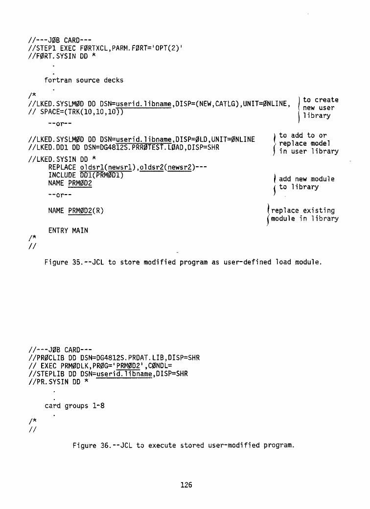
// J0B CARD //STEP1 EXEC F0RTXCL,PARM.F0RT='OPT(2)'//F0RT.SYSIN DO *
fortran source decks
/*//LKED.SYSLM0D DD DSN=userid.1ibname,DISP=(NEW,CATLG).UNIT=0NLINE. // SPACE=(TRK(10,10,10))
--or
//LKED.SYSLM0D DD D$N=userid.libname.DI$P=0LD,UNIT=0NLINE //LKED.DD1 DD DSN=DG4812S.PRR0TEST.L0AD,DISP=SHR//LKED.SYSIN DD *
REPLACE oldsrl(newsrl),oldsr2(newsr2) INCLUDE DDKPRM0D1) NAME PRM0D2--or
NAME PRM0D2(R)
to create new user library
to add to or replace model> icpictue uiuue i
) in user library
| add new module / to library
(replace existing (module in library
/* //
ENTRY MAIN
Figure 35. JCL to store modified program as user-defined load module.
// J08 CARD //PR0CLIB DD DSN=DG4812S.PRDAT.LIB,DISP=SHR // EXEC PRM0DLK,PR0G= i PRM0D2',C0NDL= //STEPLIB DD DSN=userid.libname,DISP=$HR //PR.SYSIN DD *
card groups 1-8
/*//
Figure 36.--JCL to execute stored user-modified program.
126

REFERENCES
Anderson, E. A., 1968, Development and testing of snow pack energy balance equations: Water Resources Research, v. 4, no. 1, p. 19-38.
Barry, R. G. , 1972, Climatic environment on the east slope of the Colorado front range: Boulder, University of Colorado, Institute of Arctic and Alpine Research Occasional Paper 3, 206 p.
Bassett, Gilbert, and Koenker, Roger, 1978, Asymptotic theory of least abso lute error regression: Journal of the American Statistical Association, v. 73, p. 618-622.
Beck, J. V., and Arnold, K. J. , 1977, Parameter estimation in engineering and science: New York, John Wiley and Sons, Inc., 501 p.
Box, G. E. P., and Jenkins, G. M. , 1976, Time series analysis Forecasting and control: San Francisco, Holden-Day, 575 p.
Dawdy, D. R. , Lichty, R. W. , and Bergmann, J. M. , 1972, A rainfall-runoff simulation model for estimation of flood peaks for small drainage basins: U.S. Geological Survey Professional Paper 506-B, p. B1-B28.
Dawdy, D. R. , and O'Donnell, Terence, 1965, Mathematical models of catchment behavior: Proceedings of the American Society of Civil Engineers, Journal of the Hydraulics Division, v. 91, no. HY4, p. 123-137.
Dawdy, D. R., Schaake, J. C., Jr., and Alley, W. M., 1978, Distributed routing rainfal1-runoff model: U.S. Geological Survey Water-Resources Investiga tions 78-90, 151 p.
Dickinson, W. T. , and Whiteley, H. Q. , 1970, Watershed areas contributing to runoff: International Association of Hydrologic Sciences Publication 96, p. 1.12-1.28.
Draper, N. R. , and Smith, Harry, 1966, Applied regression analysis: New York, John Wiley and Sons, Inc., 407 p.
Federer, Anthony C. , and Lash, Douglas, 1978, Brook: A hydrologic simulation model for eastern forests: Durham, New Hampshire, University of New Hampshire, Water Resources Research Center, Research Report No. 19, 84 p.
Frank, E. C., and Lee, Richard, 1966, Potential solar beam irradiation on slopes: U.S. Department of Agriculture, Forest Service Research Paper RM-18,116 p.
Green, W. H. , and Ampt, G. A., 1911, Studies on soil physics, I Flow of air and water through soils: Journal of Agricultural Research, v. 4, p. 1-24.
Hamon, W. R. , 1961, Estimating potential evapotranspiration: Proceedings of the American Society of Civil Engineers, Journal of the Hydraulic Division, v. 87, no. HY3, p. 107-120.
Hewlett, J. D. , and Nutter, W. L., 1970, The varying source area of stream- flow from upland basins, in Symposium on Interdisciplinary Aspects of Watershed Management, Montana State University, Bozeman, Montana, 1970, Proceedings, p. 65-83.
Hiemstra, L. A. V., and Francis, D. M. , 1981, Run hydrographs for prediction of flood hydrographs: Proceedings of the American Society of Civil Engineers, Journal of the Hydraulics Division, v. 107, no. HY6, p. 759-778.
Hjelmfelt, A. T., Piest, R. P., and Saxton, K. E., 1975, Mathematical modeling of erosion on upland areas: Congress of the 16th International Associ ation for Hydraulic Research, Sao Paulo, Brazil, 1975, Proceedings, v. 2, p. 40-47.
127
Hoaglin, D. C. , and Welsch, R. E. , 1978, The hat matrix in regression and ANOVA: The American Statistician, v. 32, no. 1, p. 17-22.
Hutchinson, N. E. , compiler, 1975, WATSTORE--National water data storage and retrieval system of the U.S. Geological Survey User 1 s Guide, U.S. Geological Survey Open-File Report 75-426, 791 p.
Jensen, M. E. , and Haise, H. R. , 1963, Estimating evapotranspiration from solar radiation: Proceedings of the American Society of Civil Engineers, Journal of Irrigation and Drainage, v. 89, no. IR4, p. 15-41.
Jensen, M. E., Rob, D. C. N., and Franzoy, C. E., 1969, Scheduling irrigations using climate-crop-soil data: National Conference on Water Resources Engineering of the American Society of Civil Engineers, New Orleans, La., 1969, Proceedings, 20 p.
Larson, L. W., and Peck, E. L., 1974, Accuracy of precipitation measurements for hydro!ogic modeling: Water Resources Research, v. 10, no. 4, p. 857-863.
Leaf, C. F., 1966, Free water content of snowpack in subalpine areas: Western Snow Conference, Seattle, Wash., 1966, Proceedings, v. 34, p. 17-24.
Leaf, C. F. , and Brink, G. E. , 1973, Hydrologic simulation model of Colorado subalpine forest: U.S. Department of Agriculture, Forest Service Research Paper RM-107, 23 p.
Leavesley, G. H. , and Striffler, W. D. , 1978, A mountain watershed simulation model, in Colbeck, S. C. , and Ray, M. , eds., Modeling of Snow Cover Runoff, Hanover, New Hampshire, 1978, Proceedings: U.S. Army Corps of Engineers, Cold Regions Research and Engineering Laboratory, p. 379-386.
Led ere, Guy, and Schaake, J. C. , Jr. , 1973, Methodology for assessing the potential impact of urban development on urban runoff and the relative efficiency of runoff control alternatives: Massachusetts Institute of Technology, Ralph M. Parsons Laboratory Report 167, 257 p.
Linsley, R. K. , Jr., Kohler, M. A., and Paulhus, J. L. , 1958, Hydrology for engineers: New York, McGraw-Hill, p. 151-155.
McCuen, R. H. , 1973, The role of sensitivity analysis in hydrologic modeling, Journal of Hydrology, v. 18, p. 37-53.
Mein, R. G. , and Brown, B. M. , 1978, Sensitivity of optimized parameters in watershed models: Water Resources Research, v. 14, no. 2, p. 299-303.
Miller, D. H., 1959, Transmission of insolation through pine forest canopy as it effects the melting of snow: Mitteilungen der Schweizerischen Anstalt fur das forstliche Versuchswesen, Versuchsw. Mitt., v. 35, p. 35-79.
Murray, F. W., 1967, On the computation of saturation vapor pressure: Journal of Applied Meteorology, v. 6, p. 203-204.
Musser, John J., 1963, Description of physical environment and of strip-mining operations in parts of Beaver Creek basin, Kentucky: U.S. Geological Survey Professional Paper 427-A, 25 p.
Obled, Charles, and Rosse, B. B., 1977, Mathematical models of a melting snowpack at an index plot: Journal of Hydrology, no. 32, p. 139-163.
Philip, J. R. s 1954, An infiltration equation with physical significance: Soil Science Society of America Proceedings, v. 77, p. 153-157.
Riley, J. P., Israelsen, E. K., and Eggleston, K. 0., 1973, Some approaches to snowmelt prediction, in The role of snow and ice in hydrology: Interna tional Association of Hydrological Sciences Publication 107, p. 956-971.
128

Rosenbrock, H. H. , 1960, An automatic method of finding the greatest or least value of a function: Computer Journal, v. 3, p. 175-184.
SAS Institute Inc., 1982, SAS user's guide basics, 1982 edition: Gary, N.C., Statistical Analysis System Institute Inc. , 923 p.
Sen, P. K. , 1968, Asymptotic normality of sample quantiles for independent processes: Annals of Mathematical Statistics, v. 39, p. 1724-1730.
Smith, R. E. , 1976, Field test of a distributed watershed erosion/sedimenta tion model, in Soil erosion Prediction and control: Ankeny, Iowa, Soil Conservation Society of America, p. 201-209.
Sorooshian, Soroosh, and Dracup, John, 1980, Stochastic parameter estimation procedures for hydrologic rainfall-runoff models Correlated and hetero- scedastic error cases: Water Resources Research, v. 16, no. 2, p. 430-442.
Swift, Lloyd W. , Jr. , 1976, Algorithm for solar radiation on mountain slopes: Water Resources Research, v. 12, no. 1, p. 108-112.
Tangborn, W. V., 1978, A model to predict short-term snowmelt runoff using synoptic observations of streamflow, temperature, and precipitation in Colbeck, S. C. , and Ray, M. , eds. , Modeling of snow cover runoff, Hanover, New Hampshire, 1978, Proceedings: U.S. Army Corps of Engineers, Cold Region Research and Engineering Laboratory, p. 414-426.
Thompson, E. S. , 1976, Computation of solar radiation from sky cover: Water Resources Research, v. 12, no. 5, p. 859-865.
U.S. Army, 1956, Snow hydrology: Portland, Oreg., U.S. Army Corps of Engi neers, North Pacific Division, 437 p.
U.S. Geological Survey, 1970, U.S. Geological Survey computer user's manual: Computer Center Division [Information Services Division], p. 5.4-5.7.
U.S. Soil Conservation Service, 1971, SCS national engineering handbook, Section 4 Hydrology: Washington, D.C., U.S. Government Printing Office, 654 p.
Vezina, P. E., and Pech, G. Y., 1964, Solar radiation beneath conifer canopies in relation to crown closure: Forest Science v. 10, no. 4, p. 443-451.
Weeks, W. D. , and Hebbert, R. H. E. , 1980, A comparison of rainfall-runoff models: Nordic Hydrology, v. 11, p. 7-24.
Willen, D. W. , Shumway, C. A., and Reid, J. E. , 1971, Simulation of daily snow water equivalent and melt: Western Snow Conference, Billings, Montana, 1971, Proceedings, v. 39, p. 1-8.
Woolhiser, D. A., Hanson, C. L. , and Kuhlman, A. R. , 1970, Overland flow on rangeland watersheds: Journal of Hydrology, v. 9, no. 2, p. 336-356.
Zahner, R., 1967, Refinement in empirical functions for realistic soil- moisture regimes under forest cover, in Sopper, W. E. , and Lull, H. W., eds. , International symposium of forest hydrology: New York, Pergamon Press, p. 261-274.
129

ATTACHMENT I
PRMODEL Cataloged Procedure
A cataloged procedure has been written that includes all of the JCL required to use the Precipitation-Runoff Modeling System. This procedure, named PRMODEL, is stored in the procedure library DG4812S.PRDAT.LIB. Figure 1-1 is a listing of PRMODEL.
ATTACHMENT II
Simulation Examples
The simulation examples for this attachment were developed using the Cane Branch watershed located in the Cumberland Plateau physiographic section of southeastern Kentucky. The watershed is described by Musser (1963). It has an area of 429 acres and relief of about 400 feet. The highest altitude above mean sea level is about 1,380 feet. Except for a small area of strip mining, the watershed is completely forested with a mix of hardwoods and pines. Soils generally are silt loam in texture. The topography and channel network of Cane Branch are shown in figure II-l. For daily mean flow simulation, the watershed was divided into seven HRU's. HRU 7 is the 27.4-acre strip-mined area. For stormflow simulation, an average overland-flow plane was defined in each HRU and reused several times to describe the flow plane network of each HRU. The channel system was delineated into 28 segments. The HRU and ttie channel segments defined are shown in figure II-2. A listing of the input card deck created to run a daily and stormflow simulation on Cane Branch from February 16, 1956, to September 30, 1957, is given in figure II-3, The deck consists of card groups 1, 2, 3, and 4, and includes the cards necessary for water and sediment routing of five storms. Card group 1 contains the physical description of the HRU's shown in figure II-2 and card groups 3 and 4 contain the physical description of the overland-flow plane and channel segments shown.
Selected segments of the output from this simulation run are shown in figures II-4 through II-9. The summary of the input data as they are dis played to the user in the model output is shown in figure II-4. It is impor tant that the user always review this section of the output to ensure that the data supplied in the input card groups are correct. The daily mean flow summary table and the annual summary for water year 1956 are shown in figure II-5. Note that the simulation began in February; therefore, the annual summary is for a period less than 1 year. The line printer plot of the daily mean flows for the period February and March 1956 is shown in figure 11-6. The plot is on a semi log scale.
The summary for water and sediment discharge for the five storms simulat ed is shown in figure I1-7. There were no observed sediment data available for this example. Therefore, the sediment parameters used in card group 3 were just estimated values to permit the generation of a sediment summary and a sediment-concentration graph. The stormflow hydrograph for storm no. 2 (March 13-14, 1956) is shown in figure II-8, and the hypothetical sediment- concentration graph for this storm is shown in figure II-9.
130

//PRMODEL PROC INFILE=NULLFILE,DVOUT=NULLFILE,DVLREC=1656,// DVBLK=11592,UVOUT=NULLFILE,UVLREC=11604,UVBLK=12932//PR EXEC PGM=PRMOD1,REGION=600K,TIME=3//STEPLIB DD DSN=DG4812S.PRROTEST.LOAD,DISP=SHR// DD DSN=SYS1.FORTG.LINKLI3X,DISP=SHR// DD DSN=SYS1.PLIX.TRANSLIB,DISP=SHR//FT02F001 DD DUMMY//FT03F001 DD DUMMY//FT04F001 DD UNIT=SYSDK,SPACE=(TRK,(5,5)),DISP=(,DELETE)//FT05F001 DD DDNAME=SYSIN1//FT06F001-DD SYSOUT=A//FT08F001 DD UNIT=SYSDK,SPACE=(TRK,(5,5)),DISP=(,DELETE)//FT09F001 DD DISP=(,DELETE),SPACE=(128,(1000)),// DCB=(RECFM=F,LRECL=128,DSORG=DA),UNIT=SYSDK//FT10F001 DD UNIT=SYSDK,SPACE=(TRK,(5,5)),DISP=(,DELETE)//INV DD DSN=&INV,UNIT=SYSDK,DISP=(,DELETE),SPACE=(TRK,(10,1)),// DCB=(RECFM=V8S,LRECL=1472,BLKSIZE=5896,BUFNO=2)//FT11F001 DD DSN=*. INV,DISP=(OLD,DELETE),VOL=REF=*. INV//FT12F001 DD DSN=&FHS,UNIT=SYSDK,DISP=(,DELETE),SPACE^(TRK,(5,1)),// DCB=(RECFM=VBS,LRECL=656,BLKSIZE=6568,BUFNO=2)//DFHS DD DSN=&DFHS J UNIT=SYSDK,DISP=(,DELETE),SPACE=(TRK,(10,5)),/'/ DCB=(RECFM=VBS, LRECL=108, BLKSIZE=1088)//FT13F001 DD DSN=*.DFHS,DISP=(OLD,DELETE),VOL=REF=*.DFHS//UNITQ DD DSN=&UNITQ,UNIT=SYSDK,DISP=(,DELETE),SPACE=(TRK,(100,5)),// DCB=(RECFM=VB,LRECL=5820,BLKSIZE=5830,BUFNO=2)//FT14F001 DD DSN=*.UNITQ,DISP=(OLD,DELETE),VOL=REF=*.UNITQ//UNITP DD DSN=&UNITP,UNIT=SYSDK,DISP=(,DELETE),SPACE=(TRK,(100;5)),// DCB=(RECFM=VB,LRECL=5820,BLKSIZE=5830,BUFNO=2)//FT15F001 DD DSN=*.UNITP,DISP=(OLD,DELETE),VOL=REF=*.UNITP//FT17F001 DD DSN=&LATIN,DISP=(,DELETE),SPACE=(5768,(200)),/'/ DCB=(RECFM=F,BLKSIZE=5760,DSORG=DA),UNIT=SYSDK//QSFILE DD DSN=&SFILE,DISP=(,DELETE),UNIT=SYSDK,SPACE=(TRK,(100.5)),// DCB=(RECFM=VBS,LRECL=5764,BLKSIZE=12000,3UFNO=3)//FT18F001 DD DSN=*.QSFILE,DISP=(OLD,DELETE),VOL=REF=*.QSFILE//FT20F001 DD DSN=&DVOUT,DISP=(NEW,CATLG),SPACE=(TRK,(5,5),RLSE),// DCB=(RECFM=FB,LRECL=£DVLREC,BLKSIZE=&DVBLK,BUFNO=2),// UNIT=ONLINE//FT21F001 DD DSN=&UVOUT,DISP=(NEW,CATLG),SPACE=(TRK,(5,5),RLSE) >// DCB=(RECFM=VB,LRECL=&UVLREC,BLKSIZE=&UVBLK,BUFNO=2),// UNIT=ONLINE//DISK DD DSN=&INFILE,DISP=SHR,UNIT=ONLINE,// OCB=(RECFM=VB,LRECL=11604,BLKSIZE=12932,// KEYLEN=28,DSORG=IS)//FT30F001 DD UNIT=SYSDK f SPACE=(TRK,(5,5)) f DISP=(,DELETE)//FT22F001 DD DDNAME=SYSIN2//FT23F001 DD DDNAME=SYSIN3//FT24F001 DD DDNAME=SYSIN4//FT25F001 DD DDNAME=SYSIN5//SYSPRINT DD SYSOUT=A
Figure 1-1. Cataloged procedure PRMODEL.
131

34°27' I
34°26'30' 84°26'
36° 52'
EXPLANATION
...^ Drainage boundary
A Stream gaging station
Strip mined area
5CO 500 10OO FEET _;_______j
Figure II-l. Topography and channel network of Cane Branch watershed.
132

36'
52
36C SI- 30'
84°27 P I
84°26'
500 500 1000 FEET
^ Hydrologic-response**'"~ unit (HRU) boundary
Q Hydrologic- response unit (HRU) number
CH15 Channel segment number
J13 Junction segment number
A Stream gaging station
Figure II-2. HRU and channel segments delineated for Cane Branch watershed,
133
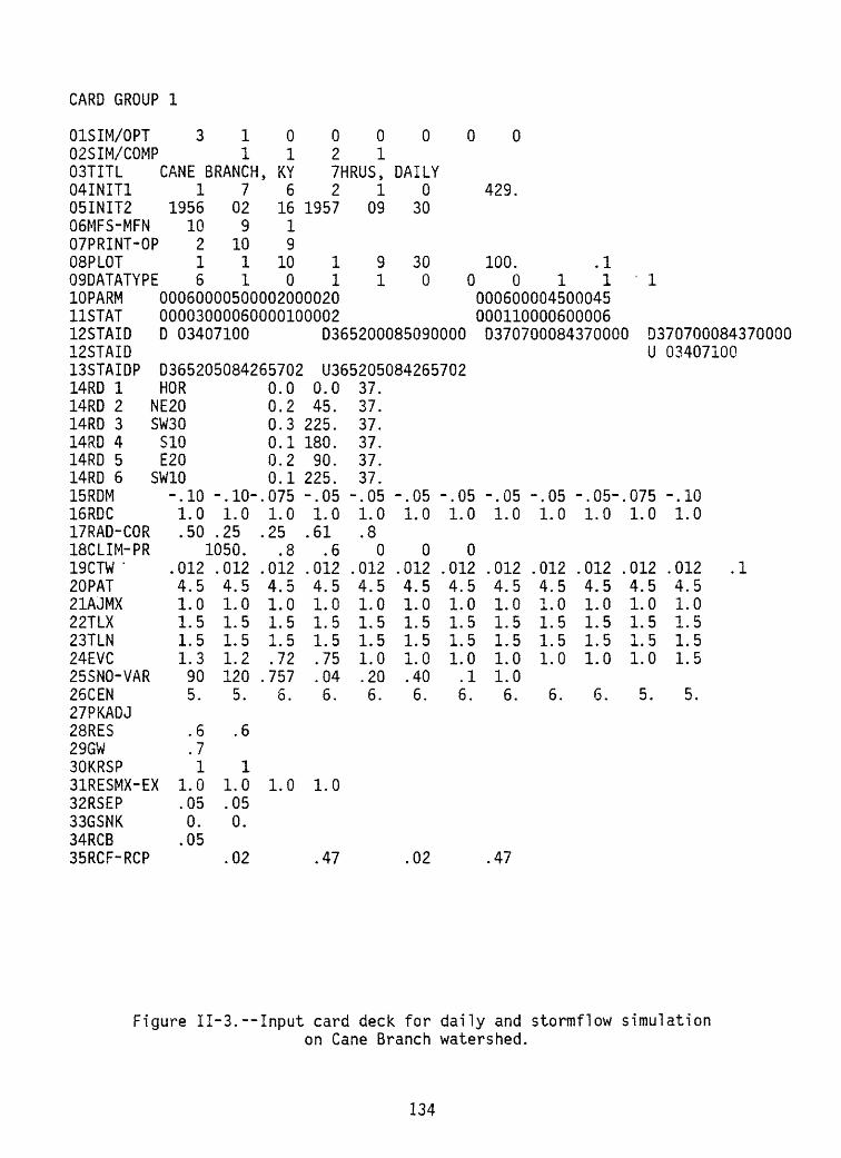
CARD GROUP 1
01SIM/OPT 31000 02SIM/COMP 1121 03TITL CANE BRANCH, KY 7HRUS, 04INIT1 17621 05INIT2 1956 02 16 1957 09 06MFS-MFN 10 9 1 07PRINT-OP 2 10 908PLOT 1 1 10 1 909DATATYPE 6101110PARM 0006000050000200002011STAT 00003000060000100002
000
DAILY 0 429.
30
300
100. .10011
000600004500045000110000600006
12STAID D 03407100 D365200085090000 D37070008437000012STAID
1
D370700084370000U 03407100
13STAIDP D365205084265702 U36520508426570214RD 1 HOR 0.0 0.0 37.14RD 2 NE20 0.2 45. 37.14RD 3 SW30 0.3 225. 37.14RD 4 S10 0.1 180. 37.14RD 5 E20 0.2 90. 37.14RD 6 SW10 0.1 225. 37.15RDM -.10 -.10-. 075 -.05 -.0516RDC 1.0 1.0 1.0 1.0 1.017RAD-COR .50 .25 .25 .61 .818CLIM-PR 1050. .8 .6 019CTW .012 .012 .012 .012 .01220PAT 4.5 4.5 4.5 4.5 4.521AJMX 1.0 1.0 1.0 1.0 1.022TLX 1.5 1.5 1.5 1.5 1.523TLN 1.5 1.5 1.5 1.5 1.524EVC 1.3 1.2 .72 .75 1.025SNO-VAR 90 120 .757 .04 .2026CEN 5. 5. 6. 6. 6.27PKADJ28RES .6 .629GW . 730KRSP 1 131RESMX-EX 1.0 1.0 1.0 1.032RSEP .05 .0533GSNK 0. 0.34RCB . 0535RCF-RCP .02 .47
-.051.0
0.0124.51.01.51.51.0.406.
.02
-.05 -.05 -.05 -.05-.1.0 1.0 1.0 1.0
0.012 .012 .012 .012 .4.5 4.5 4.5 4.51.0 1.0 1.0 1.01.5 1.5 1.5 1.51.5 1.5 1.5 1.51.0 1.0 1.0 1.0
.1 1.06. 6. 6. 6.
.47
0751.0
0124.51.01.51.51.0
5.
-.101.0
.012 .14.51.01.51.51.5
5.
Figure II-3.--Input card deck for daily and stormflow simulationon Cane Branch watershed.
134
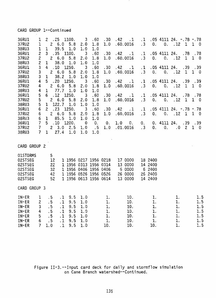
CARD GROUP 1 Continued
36RU137RU238RU336RU137RU238RU336RU137RU238RU336RU137RU238RU336RU137RU238RU336RU137RU238RU336RU137RU238RU3
111222333444555666777
CARD GROUP
01STORMS02STSEG02STSEG02STSEG02STSEG02STSEG
CARD GROUP
IN-ERIN-ERIN-ERIN-ERIN-ERIN-ERIN-ER
1234567
2 .25 1100. 3 .602 6.0 5.8 2.0 1.8
1 39.5 1.0 1.0 1.03 .35 1100. 3 .60
2 6.0 5.8 2.0 1.81 38.0 1.0 1.0 1.04 .10 1250. 3 .60
2 6.0 5.8 2.0 1.81 38.2 1.0 1.0 1.05 .20 1250. 3 .60
2 6.0 5.8 2.0 1.81 77.7 1.0 1.0 1.06 .12 1250. 3 .60
2 6.0 5.8 2.0 1.81 122.7 1.0 1.0 1.02 .23 1250. 3 .60
2 6.0 5.8 2.0 1.81 85.5 1.0 1.0 1.05 .10 1200. 0 0.
2 3.0 2.5 1.0 .51 27.4 1.0 1.0 1.0
2
512 1 1956 0217 195622 1 1956 0313 195632 1 1956 0406 195642 1 1956 0526 195652 1 1956 0613 1956
3
.5 .1 9.5 1.0
.5 .1 9.5 1.0
.5 .1 9.5 1.0
.5 .1 9.5 1.0
.5 .1 9.5 1.0
.5 .1 9.5 1.01.0 .1 9.5 1.0
.301.0
.301.0
.301.0
.301.0
.301.0
.301.0
0.1.0
02180314040605260614
1.1.1.1.1.1.
10.
.42
.60.
.42
.60.
.42
.60.
.42
.60.
.42
.60.
.42
.60.
1.0.01.
17136
2613
.10016
.10016
.10016
.10016
.10016
.10016
0.0016
00000000000000000000
10.10.10.10.10.10.10.
.1
.3
.1
.3
.1
.3
.1
.3
.1
.3
.1
.3
0..3
18146
2614
.050.
.050.
.050.
.050.
.050.
.050.
0.0.
24002400240024002400
1.1.1.1.1.1.
10.
41110.
41110.
41110.
41110.
41110.
41110.
41110.
24. -..12
24. ..12
24. ..12
24. ..12
24. ..12
24. -..12
24. ..0
1.1.1.1.1.1.1.
781
781
391
391
781
781
392
-.781 0
.781 0
.391 0
.391 0
.781 0
-,781 0
.391 0
1.1.1.1.1.1.i f
Figure II-3. Input card deck for daily and stormflow simulation on Cane Branch watershed--Continued.
135

CARD GROUP 4
NOFSEG 7020FID OF1020FID OF2020FID OF3020FID OF4020FID OF5020FID OF6020FID OF7NCRSEG 2804CHIDCH104CHIDCH2704CHIDCH2
OF6 OF6OF4 OF4OF4 OF6
04CHIDCH3 CH2 CH1 CH270F4 OF604CHIDCH4 CH3 CH104CHIDCH504CHIDCH6 CH504CHIDCH704CHIDCH8 CH7 CH6 CH104CHIDCH9 CHS CH704CHIDCH11CH9 CH7 CH404CHIDCH1204CHID J13CH12CH11CH704CHIDCH15 J13CH1204CHIDCH16CH7 CH704CHIDCH17CH16CH1504CHIDCH1804CHIDCH19CH18CH1704CHIDCH2104CHIDCH2204CHIDCH23CH21CH2104CHIDCH24CH2204CHIDCH25CH24CH2304CHIDCH26CH25CH1904CHIDCH25CH27CH2704CHIDCH29CH28CH1804CHIDCH30CH29CH26
OF4 OF6OF5 OF6OF5 OF6OF5 OF5OF5 OF6OF5 OF6OF5 OF7OF7 OF7
OF1 OF1OF2 OF2OF1 OF2OF1 OF1OF1 OF2OF2 OF2OF3 OF3OF2-OF2OF2 OF2OF2 OF2OF1 OF2OF4 OF4OF1 OF1OF1 OF2
400 2 170400 2 170400 5 530400 5 500400 3 310400 3 320400 2 200
400 31000400 2 700400 31000400 3 860400 2 650400 3 900400 41100400 41100400 2 600400 2 500400 2 660400 2 500700400 41200400 2 670400 2 500400 2 560400 2 600400 2 560400 3 780400 2 410400 3 770400 2 420400 2 660400 2 400400 3 850400 2 430
04CHIDCH31CH30CH18CH240F1 OF2 402 2 320.
2.352.631.671.861.492.20
1.18
0.69.56.61.24.16.56.34.54.25.19.09.44
.07
.30
.07
.75
.06
.70
.53
.35
.61
.37
.04
.35
.26
.03
.03
1.67 11.67 21.67 31.67 41.67 51.67 61.67 7
1.671.671.671.671.671.671.671.671.671.671.671.67
1.671.671.671.671.671.671.671.671.671.671.671.671.671.671.67
0.0.0.0.0.0.0.
0.0.0.0.0.0.0.0.0.0.0.0.0.0.0.0.0.0.0.0.0.0.0.0.0.0.0.0.
5.5.5.5.5.5.5.
5.5.5.5.
10.5.5.5.5.
10.10.5.
10.10.5.
10.5.
10.5.5.5.5.
10.15.5.
10.15.15.
5555555
5555
105555
10105
10105
105
105555
10155
101560
Figure II-3. Input card deck for daily and stormflow simulation on Cane Branch watershed Continued.
136

CANE BRANCH, KY 7HRUS
IOPT= IDOUT=
IPET= NYR=
ISIM= IUOUT=
ISSR1= NDS=
BYR/BMO/BDY= 195S/ 2/15
IOBS= 1 SCODE=319
MRDC= NRU=
ISEN= ICBC=
ISUN= NRD=
EYR/EMO/EDY= 1957/ 9/30
IPSW=
NRES= NGW= NSTOR= DAT= 429.00
MFS= 10 MFN= 9DATA TYPE
DAILY DISCHARGEDAILY EVAPDAILY MAX TEMPDAILY MIN TEMPDAILY SOLAR RADUSER VARIABLE 1USER VARIABLE 2UNIT DISCHARGEDAILY PRECIP
PARAMETERCODE
00060000500002000020
0006000045
STATISTICCODE
00003000060000100002
0001100006
UNIT PRECIP 00045 00006
STATION ID 1
03407100365200085090000370700084370000370700084370000
03407100365205084265702
365205084265702
POT SOLAR RADIATIONHOR
NE20SW30S10E20
SW10
374.4 398.6 440.2 '499.1 571.5 651.1 732.4 809.8 877.2 933.2 975.4 1003.7 1019.7260.2536.4458.8376.5433.7
284.6558.4482.2400.5457.4
327.0595.2521.7441.6497.5
388.6645.6576.7499.7553.7
466.4704.7642.8571.1621.9
554.6765.8713.6649.4695.3
547.9824.2783.7729.3769.0
739.7875.4848.2805.1837.4
823.0915.7902.4871.0895.5
894.6945.8945.7925.7942.5
950.6965.8977.0966.8977.0
989.2 1011.4977.8 984.1997.4 1008.6994.3 1009.8999.7 1012.2
RDM(1-12)= -0.10 -0.10 -0.08 -0.05 -0.05 -0.05 -0.05 -0.05 -0.05 -0.05 -0.08 -0.10RDC(1-12)= l.OC 1.00 1.00 1.00 1.00 1.00 1.00 1.00 1.00 1.00 1.00 1.00
MRDC= 2 PARS= 0.50 PARW= 0.25 RDB= 0.25RDP= 0.61RDMX= 0.80
SUNLIGHT HOURS/12HOR
NE20SW30S10E20
SW10
0.8 0.7 0.8 0.8 0.7 0.8
0.8 0.7 0.8 0.8 0.7 0.8
0.8 0.7 0.8 0.8 0.8 0.8
0.9 0.8 0.8 0.9 0.8 0.8
0.9 0.8 0.9 0.9 0.8 0.9
1.0 0.9 0.9 1.0 0.9 0.9
1.0 0.9 0.9 1.0 0.9 1.0 1.0
1.1 1.01.01.11.01.1
1.1 1.11.01.1 1.1 1.1
1.21.1 1.1 1.1 1.1 1.1
1.2 1.21.11.21.11.2
1.21.21.11.21.11.2
Figure II-4. Variables, parameters, and initial conditions for daily and stormflow simulation onCane Branch watershed.
137

CANE BRANCH, KY 7HRUS
CSEL= 1050. RMXA= 0.80 RMXM= 0.60 MTSS= 0 M1SE= 0
MPCS= 0 MPCN= 0 MPC1= 0 PCONR= 1.00 PCONS= 1.00
CTS(1-12)=0.0120000.0120000.0120000.0120000.0120000.0120000.0120000.0120000.0120000.012GOOO.0120000.012000 CTV= 0.10
PAT(1-12)= AJMX(1-12)=
TLX(1-12)= TLN(1-12)=
EVC(1-12)=
ISP1= 90
CECN(1-12)=
RES-RSEP
4.50 1.00
1.50 1.50
1.300
I5P2=12
5.00
1-
4.50 1.00
1.50 1.50
1.200
4.50 4 1.00
1.50 1 1.50 1
0.720 0.
0 EAIR= 0.757
5.00
0.60
6.00
0.05 2-
.50 4.50 1.00 1.00
.50 1.50
.50 1.50
750 1.000
FWCAP= 0.
6.00 6.00
0.60 0
4.50 1.00
1.50 1.50
1.000
4.50 1.00
1.50 1.50
1.000
04 DENI= 0.20
6.00
.05
6.00
4.50 1.00
1.50 1.50
1.000
4.50 1.00
1.50 1.50
1.000
DENMX= 0.40
6.00 6.00
4.50 1.00
1.50 1.50
1.000
4.50 1.00
1.50 1.50
1.000
SETCON= 0.
6.00 5.00
4.50 1.00
1.50 1.50
1.500
10 8ST= 1.00
5.00
RESMX-REXP 1.0000 1.0000 1.0000 1.0000
KRSP= 1 1
RCF-RCP 1- 0.0200000 0.4700000 2- 0.0200000 0.4700000
GW-GSNK 1- 0.700 0.000
RGB 1- 0.0500
Figure II-4. Variables, parameters, and initial conditions for daily and stormflow simulation onCane Branch watershed Continued.
138

CANE BRANCH, KY 7HRUS
IRU
1
2
3
4
5
6
7
IRU1234567
TOTAL
IRD
ELEV
21100.
31100.
41250.
51250.
61250.
21250.
51200.
IDS1111I11
ITST ITSW
ITNO CTX
4 111 24.004 111 24.004 111 24.004 111 24.004 111 24.004 111 24.004 111 24.00
SLOPE0.250.350.100.200.120.230.10
TXAJ
TNAJ
-0.78-0.780.780.780.390.390.390.390.780.78
-0.78-0.780.390.39
AREA39.538.038.277.7
122.785.527.4
429.0
RNSTS SNST
RNSTW TRNCF
0.10 0.100.05 0.420.10 0.100.05 0.420.10 0.100.05 0.420.10 0.100.05 0.420.10 0.100.05 0.420.10 0.100.05 0.420.00 0.000.00 1.00
PERVAREA39.538.038.277.7
122.785.527.4
429.0
COVDS
COVOW
0.600.300.600.300.600.300.600.300.600.300.600.300.000.00
IMPERVAREA
0.00.00.00.00.00.00.0
0.0
ICOV
ISOIL
3o
323232323202
SMAX
SMAV
6.005.806.005.806.005.806.005.806.005.806.005.803.002.50
UPCOR1.001 001.001.001.001.001.00
1111111
REMX
RECHR
2.001.802.001.802.001.802.001.802.001.802.001.801.000.50
DRCOR.00.00.00.00.00.00.00
SCN
SCI
O.OQ1600.300000.001600.3COOO0.001600.300000.001600.300000.001600.300000.001600.300000.001600.30000
DSCOR1.001.001.001.001.001.001.00
SRX
sex
1.000.601.00C.601.000.601.000.601.000.601.000.601.000.01
TST0.00.00.00.00.00.00.0
RETIP
IMPRV
0.000.000.000.000.00o.oc0.000.000.000.000.000.000.000.00
SEP
KSTOR
0.120
0.120
0.120
0.120
0.120
0.120
0.000
K.RES
KGW
111^1111]1112T^
Figure II-4. Variables, parameters, and initial conditions for daily and stormflow simulation onCane Branch watershed Continued.
139

BYR= 1956 BMO= 2 BDY= 16 NSP= 5
1 11956 2171956 218 NE= 162 11956 3131956 314 NE= 163 11956 4 61956 4 6 NE= 164 11956 5261956 526 NE= 165 11956 6131956 614 NE= 16
INV=1956 INV=1957
STORMFLOW HYDROGRAPH PARAMETERS FOR EACH HYDROLOGIC RESPONSE UNIT(IRU)
IRU KSAT PSP RGF DRN KR HC KF MM EN1 0.500 0.100 9.500 1.000 1.00 10.0 1.00000 1.00 1.502 0.500 0.100 9.500 1.000 1.00 10,0 1.00000 1.00 1.503 0.500 0.100 9.500 1.000 1.00 10.0 1.00000 1.00 1.504 0.500 0.100 9.500 1.000 1.00 10.0 1.00000 1.00 1.505 0.500 0.100 9.500 1.000 1.00 10.0 1.00000 1.00 1.506 0.500 0.100 9.500 1.000 1.00 10.0 1.00000 1.00 1.507 1.000 0.100 9.500 1.000 10.00 10.010.00000 1.00 1.50
WY WYD #HS ST# RFL SFL BEGIN AND END TIMES FOR #HS1956195619561956195619561956
140141165166189239257
1111111
1122345
0101000
1010001
0.0.0.0.0.0.0.
1440.1440.1440.1440.1440.1440.1440.
1956 258 1 5 1 0 0.1440.
Figure II-4. Variables, parameters, and initial conditions for daily and stormflow simulation enCane Branch watershed Continued.
140

NUMBER O
F OVERLAND FlOW PLANE
SEGMENTS IS
7.
THEI
R CHARACTERISTICS
ARE
AS FOLLOWS:
SEGM
ENT
# NAME
1 OF1
2 OF2
3 OF3
4 OF
45 OF5
6 OF6
7 OF7
NUMBER O
F
SEGM
ENT
# NA
ME1
CH1
2 CH
273
CH2
4 CH3
5 CH4
6 CH
57
CH6
8 CH7
9 CH8
10 CH9
11 CH
1112 CH12
13
J13
U CH15
15 CI
I16
16 C
II17
17 CH18
18 C
H19
19 CI
I21
20 CH22
21 CH23
22 CI
I24
23 CH25
24 CH
2625
CH28
26 CH29
27 CH30
28 CH31
IDS 1 1 1 1 1 1 1 CHAN
NEL
AND
UPSTREAM
SEGMENTS
CH2
CH3
CH5
CH7
CH8
CH9
CIIJ2
J13
CH7
CH16
CH18
CH21
CH22
CH24
CH25
CH27
CII2
8CH29
CH30
CH1
cm CH6
CH?
CH7
CH11
CH12
CH7
CH15
CH17
CH21
CH23
CH19
CH27
CH18
CH26
CH18
IRU 1 2 3 4 5 6 7
RESE
RVOI
RSEGMENTS
ADJA
CENT
SEGM
ENTS
OF6
OF4
OF4
CH27
OF4
OF4
OF5
OF5
OF5
CH1
OF5
OF5
CII4
OF
5OF
7CH
7OF
1OF2
OF1
OF1
OF1
OF2
OF3
OF2
OF2
OF2
OF1
OF4
OF1
OF1
OF1
OF6
OF4
OF6
OF6
ore
OF6
OF6
OF5
OF6
OF6
OF7
OF7
OF1
OF 2
OF2
OF1
OF 2
OF2
OF3
OF2
OF2
OF2
OF2
OF4
OF1
OF2
OF2
IS
28
INC.
AREA 14
.716
.118
.816
.212
.213
.015
.915
.7 8.7
7.2
7.7
4.6
0.0
9.4
5.2
3.9
4.4
4.7
4.4
19.0 3.2
6.0
3.3
5.2
9.2
6.6
3.4
2.5
THRE
SDE
PTH
0.0000
0.0000
0.0000
0.0000
0.0000
0.00
000.0000
CUM.
TH
RES
AREA
DISC.
14.7
0.
0016
.1
0.00
18.8
0.00
65.8
0.
0092
.7
0.00
13.0
0.00
28.9
0.00
15.7
0.00
68.0
0.
0090
.8
0.00
206.9
0.00
4.6
0.00
227.2
0.00
241.1
0.00
36.5
0.00
281.6
0.00
4.4
0.00
290.6
0.00
4.4
0.00
19.0
0.00
11.9
0.00
25.0
0.
0040
.2
0.00
336.0
0.00
41.3
0.00
52.3
0.00
391.
7 0.00
423.5
0.00
TYPE 4 4 4 4 4 4 4
TYPE 4 4 4 4 4 4 4 4 4 4 4 4 7 4 4 4 4 4 4 4 4 4 4 4 4 4 4 4
IN O
UT0
00
00
00
00
00
00
0
IN O
UT0
00
00
00
0.
0 0
0 0
0 0
0 0
0 0
0 0
0 0
0 0
0 0
0 0
0 0
0 0
0 0
0 0
0 0
0 0
0 0
0 0
0 0
0 0
0 0
0 0
0 0
0 2
NDX
LENGTH SL
OPE
2 170.0
.0000
2 17
0.0
.0000
5 530.0
.0000
5 500.0
.0000
3 31
0.0
.0000
3 320.0
.0000
2 20
0.0
.0000
NDX
LENG
TH SLOPE
3 10
00.0
.0
000
2 70
0.0
.000
03
1000.0 .0
000
3 86
0.0
.000
02
650.0
.0000
3 900.0
.0000
4 1100.0 .0
000
4 1100.0 .0
000
2 600.0
.0000
2 500.0
.0000
2 660. 0 .0000
2 500.0
.0000
0 0.
0 .0
000
4 1200.0 .0
000
2 67
0.0
.000
02
500.
0 .0000
2 560.0
.0000
2 600.0
.0000
2 560.0
.000
03
780.
0 .0
000
2 410.0
.0000
3 770.0
.0000
2 42
0.0
.0000
2 660.0
.000
02
400.
0 .0000
3 85
0.0
.000
02
430.
0 .0
000
2 320.0
.000
0
ROUG
HNESS .000
.000
.000
.000
.000
.000
.000
ROUGH
NESS
.000
.000
.000
.000
.000
.000
.000
.000
.000
.000
.000
.000
.000
.000
.000
.000
.000
.000
.000
.000
.000
.000
.000
.000
.000
.000
.000
.000
PARM1
PARM
2 AL
PHA
EXPM
ROUTE
INT.
INT.
2.35
1.
67
2.35 1.
67
5.0
5.0
2.63
1.
67
2.63
1.
67
5.0
5.0
1.67
1.67
1.67 1.
67
5.0
5.0
1.86
1.
67
1.86
1.
67
5.0
5.0
1.49
1.
67
1.49
1.
67
5.0
5.0
2.20
1.67
2.20 1.
67
5.0
5.0
1.18
1.67
1.18
1.6
7 5.
0 5.
0
PARM1
PARM
2 AL
PHA
EXPM
ROUTE
INT.
INT.
0.69
1.67
0.
69 1.
67
5.0
5.0
0.56
1.
67
0.56
1.
67
5.0
5.0
0.61
1.67
0.61 1.
67
5.0
5.0
0.24
1.
67
0.24
1.
67
5.0
5.0
0.16
1.67
0.16
1.
67
10.0
10
.00.
56
1.67
0.
56 1.
67
5.0
5.0
0.34
1.
67
0.34
1.
67
5.0
5.0
0.54
1.67
0.54
1.
67
5.0
5.0
0.25
1.67
0.
25 1.
67
5.0
50
0.19
1.67
0.
19 1.
67
10.0
10
.00.
09
1.67
0.09
1.
67
10.0
10
.00.
44
1.67
0.44
1.
67
5.0
5.0
0.00
0.
00
0.44
1.
67
10.0
10
.00.
07
1.67
0.
07 1.
67
10.0
10
.00.
30
1.67
0.30 1.
67
5.0
5.0
0.07
1.
67
0.07
1.67
10.0
10.0
0.75
1.67
0.75
1.
67
5.0
5.0
0.06
1.67
0.06
1.
67
10.0
10
.00.70
1.67
0.70
1.
67
5.0
5.0
0.53
1.
67
0.53
1.
67
5.0
5.0
0.35
1.67
0.35 1.67
5.0
5.0
0.61
1.67
0.
61 1.
67
5.0
5.0
0.37
1.67
0.37
1.
67
10.0
10
.00.
04
1.67
0.04
1.
67
15.0
15.0
0.35
1.67
0.35
1.
67
5.0
5.0
0.26
1.67
0.26
1.
67
10.0
10
.00.03
1.67
0.03 1
.67
15.0
15
.00.03
1.67
0.
03 1.
67
15.0
60.0
Figure II
-4.-
-Var
iabl
es,
parameters,
and
init
ial
cond
itio
ns for
daily
and
stormflow
simu
lati
on on
Cane
Branch watershed Continued

OBSE
RVED
AN
D PREDICTED
RUNO
FF FOR
WY 1956
DAY
OCTO
BER
NOVE
MBF.
R DFCEMBER
JANU
ARY
FEBRUARY
MARCH
OBS
PREO
DBS
PRED
OB
S PR
ED
OBS
PRED
08S
PRED
OB
S PR
ED
1 2 3 4 5 6 7 0 9 10 11 12 13 14 15 16 17 18 19 20 21 22 23 24 25 26 27 28 29 30 31
0.00
0.00
0.00
0.00
0.00
0.00
0.00
0.00
0.00
0.00
0.00
0.00
0.00
0.00
0.00
0.00
0.00
0.00
0.00
0.00
0.00
0.00
0.00
0.00
0.00
0.00
0.00
0.00
0.00
0.00
0.00
0.00
0.00
0.00
0.00
0.00
0.00
0.00
0.00
0.00
0.00
0.00
0.00
0.00
0.00
0.00
0.00
0.00
0.00
0.00
0.00
0.00
0.00
0.00
0.00
0.00
0.00
0.00
0.00
0.00
0.00
0.00
0.00
0.00
0.00
0.00
0.00
0.00
0.00
0.00
0.00
0.00
0.00
0.00
0.00
o.oo
0.00
0.00
0.00
0.00
0.00
0.00
0.00
0.00
0.00
0.00
0.00
0.00
0.00
0.00
0.00
0.00
0.00
0.00
0.00
o.oo
0.00
0.00
0.00
0.00
0.00
0.00
0.00
0.00
0.00
0.00
0.00
0.00
0.00
0.00
0.00
0.00
0.00
0.00
0.00
0.00
0.00
0.00
0.00
0.00
0.00
0.00
0.00
0.00
0.00
0.00
0.00
0.00
0.00
0.00
0.00
0.00
0.00
0.00
0.00
0.00
0.00
0.00.
0.00
0.00
0.00
0.00
0.00
0.00
0.00
0.00
0.00
0.00
0.00
0.00
0.00
o.co
0.00
0.00
0.00
0.00
0.00
0,00
0.00
0.00
0.00
0.00
0.00
0.00
0.00
0.00
0.00
0.00
0.00
0.00
0.00
0.00
0.00
0.00
0.00
0.00
0.00
0.00
0.00
0.00
0.00
0.00
0.00
0.00
0.00
0.00
0.00
0.00
0.00
0.00
. 0.00
0.00
0.00
0.00
0.00
0.00
0.00
0.00
0.00
0.00
0.00
0.00
0.00
0.00
0.00
0.00
0.00
0.00
0.00
0.00
0.00
0.00
0.00
0.00
0.00
0.00
0.00
0.00
0.00
0.00
0.00
0.00
0.00
0.00
0.00
0.00
0.00
0.00
0.00
0.00
0.00
0.00
0.00
0.00
0.00
0.00
0.00
0.00
0.00
0.00
0.00
0.00
0.00
0.00
0.00
0.00
0.00
0.00
0.00
0.00
0.00
0.00
0.00
0.00
0.00
0.00
0.00
0.00
0.00
0.00
0.00
0.00
0.00
3.50
25.00
25.00
7.40
6.40
2.60
1.70
1.10
2.70
5.00
3.10
2.40
2.10
1.70
0.00
0.00
0.00
0.00
0.00
0.00
0.00
0.00
0.00
0.00
0.00
0.00
0.00
0.00
0.00
0.00
0.00
3.52
18.5
324
.50
11.12
5.56
3.19
2.19
1.67
3.49
4.46
3.18
3.04
2.07
1.66
0.00
0.00
1.30
2.00
2.80
2.70
1.90
1.50
5.40
5.40
2.80
1.90
1.50
1.70
3.20
24.0
04.
805.
904.
002.80
2.80
2.50
1.50
1.40
0.88
1.30
0.88
0.88
0.78
0.73
0.78
0.60
0.52
1.63
1.73
2.66
2.00
1.62
1.39
4.74
3.27
2.26
1.75
1.48
2.62
1.94
16.61
6.46
6.18
4.23
2.85
2.02
1.62
1.37
1.20
1.07
1.71
0.95
0.88
0.81
0.96
0.73
0.67
0.63
Figure II
-5.-
-Dai
ly mean fl
ow s
umma
ry table
and
annual su
mmar
y for
daily
simu
lati
on on Ca
ne Br
anch
watershed.

a ic f»«tfj r-4 O
§ o o o o o o o o o o o o o o
aoo«3vn*
i <= a
i 1
*» 2 >J=
SI O <v">
O O O O O 3 O O O O O O UI UJ -1
ee u u.UJ 2
143

FEB IR 11 IR12 IR13 IR14 IR15 IR16 I17 I18 I19 I20 I21 I22 I23 I24 I25 I25 I27 I28 I29 I
MAR I 2 I3 I4 I5 I6 I7 I8 I9 I
10 I11 I12 I13 I14 I15 I16 I17 I18 I19 I20 I21 I22 I23 I24 I25 I26 I27 I28 I29 I30 I31 I
2 .5 1.0
! I! I! I! I! I! I! I! I! I! I! I! I! I 0! I! I; ii i! I! I
f + + . ! I! I! I! Ii i! I! I! I! I! I! I! I! I! I! I! I! I! I! I! I! I P! 0 IP'. I! OPI! * I! * I! 0 PI! PO I! 0 P I'.OP I
2.0 +_..._...._
iiiii! *iiti! 0 P
0 ! PP !
! 0 PjI *! 0 P!*
* i 0 P +-
P 0! POP 0
P 0!PO !
i! P! P 0
PO!* !
0 ! PP 0iiii'
! *P 0
P ! 0P 0 !0 !
;0 P !
iiiitti
5.0
itI;IIIi
i o! P 0iiii
p biiii. + i.jiii
P!0!0iiiiii
0! P! OP
OP !1iiiIiiiiiitii
10. 20 +
IIIIIII PII PIIIIIII1
I1
. +_ IIIIIjjIIIIII PIIIIIIIII1
J
.1
IIII1
50
0*
0-
100.* IIIIIIIIIIIIIIIIIIII«. IIIIIIIIIIIIIIIIT
IIIIIIIIIIIIT
i
Figure II-6. Line printer plot of simulated and observed daily mean discharge for Cane Branch watershed, February and March, 1956.
144

STORM PREDICTED VOLUME (INCHES)
ROUTED OBSERVEDOUTFLOW OUTFLOW(INCHES) (INCHES)
PREDICTED OBSERVEDPEAK PEAK(CFS) (CFS)
PREDICTEDSEDIMENT(TONS)
2.441.070.700.010.03
2.391.030.650.010.03
2.821.521.170.010.01
96.8364.5664.340.361.28
83.8075.0097.800.610.64
1094.26525.59451.48
2.6032.27
SUMMEAN
PERCENT
STORM VOLUME ERROR SUMMARY
ABS VALUE OBF FNC
NO LOG LOG
1.310.2623.63
SUM OF SQUARES OBF FNC
NO LOG LOG
2.270.45
0.560.11
30.14
1.370.27
SUMMEAN
PERCENT
STORM PEAK ERROR SUMMARY
ABS VALUE OBF FNC SUM OF SQUARES OBF FNC
NO LOG LOG NO LOG LOG
57.8411.5722.43
1.950.39
1399.28279.8632.44
0.990.20
Figure II-7. Summary for water and sediment discharge for five storms simulated on Cane Branch watershed.
145

CANE BRANCH, KY 7HRUS , DISCHARGE IN CFSSEGMENT CH31 OUT 3/13/1956 - 3/14/1956
PREDICTED (P), OBSERVED (0), BOTH (*), OUT OF PLOT RANGE (R) VALUE = PREDICTED DIVIDED BY 10 TO THE APPROPRIATE POWER
0.0100 0.1000 1.000 10.00 100.C TIME VALUE \ 2 | 4 { 6 | 8 ! | 2 !4!6J8|! 2 | 41618!! 2 | 4 | b ! 8 100 2.5910. . . ....... . . ....... . P 0 ....... . . .....
P 0 P 0
P 0 P 0
P 0 P 0
P 0 P 0 P 0
....... . . ....... P.O. ....... . . . . . . .P 0 P 0 P 0 P 0 P 0
P 0 P 0 P 0 P 0
200300400500600700800900100011001200130014001500160017001800190020002100220023002400100200300400500600700800900
100011001200130014001500160017001800190020002100220023002400
2.45642.27622.11331.90121.73351. 65671. 62841.61311.60001.5874.1.57511.56301.55111.53941. 52801.51671. 50571. 49491.48741.5390.1.84022.86515.38711. 17101.82621.96161.62991.29512.93265.0668.3.87172. 31791.76521.52421.38731.29281. 21871. 15641. 10181.0528.1.00820.96710.92900.89358.60338.29248,0002
0 P C
P 0 P 0
P 0 P 0
P 0. . P .0. P 0
P 0 P 0
P 0 P 0
P 0 P 0
P 0PO *
OP OP
0 P 0 P 0 P
0 PFigure II-8.--Line printer plot of simulated and observed discharge for
storm 2 (March 13-14, 1956) on Cane Branch watershed.
146

CANE BRANCH, KY 7HRUS , , SEDIMENT IN G/LSEGMENT CH31 OUT 3/13/1956 - 3/14/1956
PREDICTED (P), OBSERVED (0), BOTH (*), OUT OF PLOT RANGE (R) VALUE = PREDICTED DIVIDED BY 10 TO THE APPROPRIATE POWER
0.0100 0.1000 1.000 10.00 100.0TIME VALUE J 2 ! 4 | 6 | 8 11 2 !4|6j8ii 2 J4i6',8!! 2 |416i8
100 O.OOOOR . . ....... . . ....... . . ....... . . . . . . .200 O.OOOOR300 O.OOOOR400 O.OOOOR500 O.OOOOR600 O.OOOOR700 O.OOOOR800 O.OOOOR900 O.OOOOR
1000 O.OOOOR1100 O.OOOOR . . ....... . . ....... . . ....... . . . . . . .1200 O.OOOOR1300 O.OOOOR1400 O.OOOOR1500 O.OOOOR1600 O.OOOOR1700 O.OOOOR1800 O.OOOOR1900 O.OOOOR2000 0.5321R2100 1.8428. . . ....... P. . ....... . . ....... . . . . . . ,2200 1.1915 P2300 3.5176 P2400 6.2298 P100 1.4944 P200 1.5493 P300 1.5306 ' P400 1.5456 P500 1.4967 P600 1.4757 P700 1.3942. . . ....... . . ....... . . ....... P . . . . . . .800 1.6309 P900 1.6342 P
1000 1.4864 P1100 1.2864 P1200 1.1061 P1300 0.9475 P1400 7.9204 P1500 6.3991 P1600 5.0285 P1700 3.8991. . . ....... . . ....... . . P ...... . . . . . . .1800 3.0286 P1900 2.3835 P2000 1.9124 P2100 1.5672 P2200 1.3106 P2300 1.1160 P2400 0.9651 P
Figure II-9. Line printer plot of simulated sediment concentration graph for storm 2 (March 13-14, 1956) on Cane Branch watershed.
147

Rosenbrock Optimization and Sensitivity Analysis Example
An example of selected segments of the input and output for a daily simulation run using the Rosenbrock optimization option followed by the sensitivity analysis option is shown in figures 11-10 through 11-14. The four parameters SMAX (LOP=8), EVC (LOP=74), RCF (LOP=50), and RCP (LOP=51) were optimized. Card groups 1, 7, and 8 are shown in figure 11-10. The input values in card group 7 for the optimization are displayed in the model output as shown in figure 11-11. An initialization period of February through September, 1956, was used and parameters were fitted only on the period October, 1956, through September,. 1957. The results of each step in the Rosenbrock optimization procedure are displayed along with the summary of best fit parameter values as shown in figure 11-12. The first line of output shows the initial objective function value in the first column followed by a zero in the second column and then four columns showing the parameter values used to obtain the initial objective function. Parameter columns are in the same order as the '05PARAM1 1 cards in card group 7. The second row begins the iterations of the optimization procedure. The first column is the iteration number and the second column is the sequence number of the parameter being adjusted. The next column is the old objective function from the previous iteration and it is followed by the objective function value computed during the current iteration. The remaining four columns are again the parameter values used in this iteration. In this example, log transforms were selected so that parameters were adjusted as a percentage of their initial value. Therefore, the tabular values are log values. This table is followed by the initial and final parameter and objective function values. Again, these values are log values. The base 10 parameter values are given in the last section of the optimization output. The values for the distributed parameters SMAX and 'EVC are output in the same sequential order as they are expressed on the '06PARAM2 1 card. If the '06PARAM2 1 card is not used, then the sequence is 1 to n, where n is the maximum number of HRU's, months, or reservoirs about which the parameter is distributed.
Using the Rosenbrock optimization option with correlation analysis produces a different output from that shown in figure 11-12. The correlation analysis option for daily simulation is selected by changing the IOPT parame ter on card 1 of card group 1 (fig. 11-10) from a "1" to a "2." Output from iterations 0 and 1 for a Rosenbrock optimization with correlation analysis is shown in figure 11-13. A table of parameter values and options precedes the output shown in figure 11-13 and is identical to the output shown in figure 11-11. Iteration 0 presents the results of the simulation run for the optimi zation period using the initial parameter values. The subiterations shown are the iterations for fitting the autoregressive moving average (ARMA) model being used to model the correlation of errors on successive days. Subiterations are terminated when no further improvement is made in the sum of squares computation which is the objective function. The ARMA parameters are shown for each subiteration. Subiteration 0 shows the objective function without the ARMA model. The final set of ARMA parameters are carried forward to the next major iteration to provide a starting point in the subiterations.
A Chi-squared statistic and the lag 1-10 correlations are presented for this major iteration for the cases of before and after ARMA model application. This is followed by the variance of the original series and the white noise
148

CARD GROUP 1
01SIM/OPT 01100 02SIM/COMP 1121 03TITL CANE BRANCH, KY 7HRUS, 04INIT1 17621 05INIT2 1956 02 16 1957 09 06MFS-MFN 10 9 1 07PRINT-OP 2 10 908PLOT 1 1 10 1 909DATATYPE 6101110PARM 0006000050000200002011STAT 00003000060000100002
0
DAILY 0
30
300
12STAID D 03407100 D36520008509000012STAID
0 0
429.
100. .10011000600004500045000110000600006
D370700084370000
1
D370700084370000U 03407100
13STAIDP D365205084265702 U36520508426570214RD 1 HOR 0.0 0.0 37.14RD 2 NE20 0.2 45. 37.14RD 3 SW30 0.3 225. 37.14RD 4 S10 0.1 180. 37.14RD 5 E20 0.2 90. 37.14RD 6 SW10 0.1 225. 37.15RDM -.10 -.10-. 075 -.05 -.0516RDC 1.0 1.0 1.0 1.0 1.017RAD-COR .50 .25 .25 .61 .818CLIM-PR 1050. .8 .6 019CTW .012 .012 .012 .012 .01220PAT 4.5 4.5 4.5 4.5 4.521AJMX 1.0 1.0 1.0 1.0 1.022TLX 1.5 1.5 1.5 1.5 1.523TLN 1.5 1.5 1.5 1.5 1.524EVC 1.3 1.2 .72 .75 1.025SNO-VAR 90 120 .757 .04 .2026CEN 5. 5. 6. 6. 6.27PKADJ28RES .6 .629GW . 730KRSP 1 131RESMX-EX 1.0 1.0 1.0 1.032RSEP .05 .0533GSNK 0. 0.34RCB . 0535RCF-RCP .02 .47
-.05 -.05 -.05 -.05 -.05-.1.0 1.
0
0 1.0 1.0 1.0
0.012 .012 .012 .012 .012 .4.5 4.1.0 1.1.5 1.1.5 1.1.0 1..40 .6. 6
.02
5 4.5 4.5 4.50 1.0 1.0 1.05 1.5 1.5 - 1.55 1.5 1.5 1.50 1.0 1.0 1.01 1.0
6. 6. 6.
.47
0751.0
0124.51.01.51.51.0
5.
-.101.0
.012 .14.51.01.51.51.5
5.
Figure 11-10.--Input card deck for a Rosenbrock optimization followed by a sensitivity analysis on Cane Branch watershed.
149

CARD GROUP I Continued
36RU137RU238RU336RU137RU238RU336RU137RU238RU336RU137RU238RU336RU137RU238RU336RU137RU238RU336RU137RU238RU3
111222333444555666777
2
13
14
15
16
12
15
1
2
2
2
2
2
2
2
.256.
39..35
6.38.
.106.
38..20
6.77..12
6.122..23
6.85..10
3.27.
1100.0 5.85 1.01100.
0 5.80 1.01250.
0 5.82 1.01250.
0 5.87 1.01250.
0 5.87 1.01250.
0 5.85 1.01200.
0 2.54 1.0
32.01.0
32.01.0
32.01.0
32.01.0
32.01.0
32.01.0
01.01.0
.601.81.0.601.81.0.601.81.0.601.81.0.601.81.0.601.81.00..5
1.0
.301.0
.301.0
.301.0
.301.0
.301.0
.301.0
0.1.0
.42
.60.
.42
.60.
.42
.60.
.42
.60.
.42
.60.
.42
.60.
1.0.01.
.10016
.10016
.10016
.10016
.10016
.10016
0.0016
.1
.3
.1
.3
.1
.3
.1
.3
.1
.3
.1
.3
0..3
CARD GROUPS 7 AND 8
010PT1020PT203IOBF040PT405PARAM105PARAM105PARAM105PARAM1010PT/SENS04SENST05PARAM105PARAM105PARAM105PARAM1010PT/SENS
19561956
248
745051048
7450510
2101811001
.0111000
161
07
1211207
1211
19561957
00001
0000
99
.1
.1
.1
.110
3030
0.0.0.0.9
10211
.05 4111 24. -.78 -.780. 0. .12 1 1 0
.05 4111 24. .78 .780. 0. .12 1 1 0
.05 4111 24. .39 .390. 0. .12 1 1 0
.05 4111 24. .39 .390. 0. .12 1 1 0
.05 4111 24. .78 .780. 0. .12 1 1 0
.05 4111 24. -.78 -.780. 0. .12 1 1 0
0. 4111 24. .39 .390. 0. .0210
Figure 11-10. Input card deck for a Rosenbrock optimization followed by a sensitivity analysis on Cane Branch watershed Continued.
150

CANE BRANCH, KY 7HRUS, DAILY
IOPT=IDOUT=
IPET=NYR=
10
12
ISIM=IUOUT=
ISSR1=NDS=
00
11
IOBS= 1SCODE=319
MRDC=NRU=
27
ISEN=ICBC=
ISUN=NRD=
00
16
IPSW=
NRES= NGW= NSTOR=
8YR/BMO/BDY= 1956/ 2/16
INIT-BYR/BMO/BDY= 1956/ 2/16 IOBF= 2 ITRANS= 1 MFS= 10 MFN= 9
EYR/EMO/EDY= 1957/ 9/30
EYR/EMO/EDY= 1956/ 9/30 OPT -BYR/BMO/BDY= 1956/10/ 1
DATA TYPE PARAMETER STATISTIC
DAILY DISCHARGEDAILY EVAPDAILY MAX TEMPDAILY MIN TEMPDAILY SOLAR RADUSER VARIABLE 1USER VARIABLE 2UNIT DISCHARGEDAILY PRECIP
CODEOOC60000500002000020
0006000045
CODE00003000060000100002
0001100006
UNIT PRECIP 00045 00006
STATION ID 1DSN406700093
03407100365200085090000370700084370000370700084370000
03407100365205084265702
8 365205084265702
DAT= 429.00
EYR/EMO/EDY= 1957/ 9/30
POT SOLAR RADIATION123456
HORNE20SW30
S10E20
SW10
374.4260.2536.4458.8376.5433.7
398.6284.6558.4482.2400.5457.4
440.2327.0595.2521.7441.6497.5
499.1388.6645.6576.7499.7553.7
571.5466.4704.7642.8571.1621.9
651.1554.6765.8713.5649.4695.3
732.4647.9824.2783.7729.3769.0
809.8739.7875.4848.2805.1837.4
877.2823.0915.7902.4871.0895.5
933.2894.6945.8945.7925.7942.5
975.4 1003.7950.6 989.2965.8 977.8977.0 997.4966.8 994.3977.0 999.7
RDM(1-12)= -0.10 -0.10 -0.08 -0.05 -0.05 -0.05 -0.05 -0.05 -0.05 -0.05 -0.08 -0.10RDC(1-12)= 1.00 1.00 1.00 l.CO 1.00 1.00 1.00 1.00 1.00 1.00 1.00 1.00
HRDC= 2 PARS= 0.50 PARW= 0.25 RDB= 0.25RDP= 0.61RDMX= 0.80
SUNLIGHT HOURS/12HOR
NE20SW30S10E20
SW10
0.80.70.80.80.70.8
0.80.70.80.80.70.8
0.80.70.80.80.80.8
0.90.80.80.90.80.8
0.90.80.90.90.80.9
1.00.90.91.00.90.9
1.00.90.91.00.91.0
1.01.01.01.01.01.0
1.11.01.01.11.01.1
1.11.11.01.11.11.1
1.21.11.11.11.11.1
1.21.21.11.21.11.2
Figure 11-11. Variables, parameters, and initial conditions for Rosenbrock optimization run on Cane Branch watershed.
151

CANE BRANCH, KY 7HRUS, DAILY
CSEL= 1050. RMXA= 0.80 RMXM= 0.60 MTSS= 0 MTSE= 0
MPCS= 0 MPCN= 0 MPC1= 0 PCONR= 1.00 PCONS= 1.00
CTS(1-12)=0.0120000.0120000.0120000.0120000.0120000.0120000.0120000.0120000.0120000.0120000.0120000.012000o.io
PAT(1-12)= AJMX(1-12)=
TLX(1-12)= TLN(1-12)=
4.50 1.00
1.50 1.50
4.50 1.00
1.50 1.50
4.50 1.00
1.50 1.50
4.50 1.00
1.50 1.50
4.50 1.00
1.50 1.50
4.50 1.00
1.50 1.50
4.50 1.00
1.50 1.50
4.50 1.00
1.50 1.50
4.50 1.00
1.50 1.50
4.50 1.00
1.50 1.50
4.50 1.00
1.50 1.50
4.50 1.00
1.50 1.50
£VC(1-12)= 1.300 1.200 0.720 0.750 1.000 1.000 1.000 1.000 1.000 1.000 1.000 1.500
ISP1= 90 ISP2=120 EAIR= 0.757 FWCAP= 0.04 DENI= 0.20 OENMX= 0.40 SETCON= 0.10 BST= 1.00
CECN(1-12)= 0.00 0.00 0.00 0.00 0.00 0.00 0.00 0.00 0.00 0.00 0.00 0.00
RES-RSEP 1- 0.60 0.05 2- 0.60 0.05
RESMX-REXP 1.0000 1.0000 1.0000 1.0000
KRSP= 1 1
RCF-RCP 1- 0.0200000 0.4700000 2- 0.0200000 0.4700000
GW-GSNK 1- 0.700 0.000
RGB 1- 0.0500
Figure 11-11. Variables, parameters, and initial conditions for Rosenbrock optimization run on Cane Branch watershed Continued.
152

CANE BRANCH, KY 7HRUS, DAILY
1RU
1
2
3
4
5
6
7
IRU1234567
TOTAL
IRD
ELEV
21100.
31100.
41250.
51250.
61250.
21250.
51200.
IDS1111111
ITST ITSW
ITND CTX
4 111 24.004 111 24.004 111 24.004 111 24.004 111 24.004 111 24.004 111 24.00
SLOPE0.250.350.100.200.120.230.10
TXAJ
TNAJ
-0.78-0.780.780.780.390.390.390.390.780.78
-0.78-0.780.390.39
AREA39.538.038.277.7
122.785.527.4
429.0
RNSTS SNST
RNSTW TRNCF
0.10 0.100.05 0.420.10 0.100.05 0.420.10 0.100.05 0.420.10 0.100.05 0.420.10 0.100.05 0.420.10 0.100.05 0.420.00 0.000.00 1.00
PERVAREA39.538.038.277.7
122.785.527.4
429.0
COVDS
COVDW
0.600.300.600.300.600.300.600.300.600.300.600.300.000.00
IMPERVAREA
0.00.00.00.00.00.00.0
0.0
ICOV SMAX
I SOIL SMAV
32323232323202
6.005.806.005.806.005.806.005.806.005.806.005.803.002.50
UPCOR1.001.001.001.001.001.001.00
REMX
RECHR
2.001.802.001.802.001.802.001.802.001.802.001.801.000.50
DRCOR1.001.001.001.001.001.001.00
SCN
SCI
0.001600.300000.001600. 300000.001600.300000.001600.300000.001600.300000.001600.300000.001600.30000
DSCOR1.001.001.001.001.001.001.00
SRX
sex1.000.601.000.601.000.601.000.601.000.601.000.601.000.01
1ST0.00.00.00.00.00.00.0
RETIP
IMPRV
0.000.000.000.000.000.000.000.000.000.000.000.000.000.00
SEP
KSTOR
0.120
0.120
0.120
0.120
0.120
0.120
0.000
KRES
KGW
1111X
111111121
Figure 11-11.--Variables, parameters, and initial conditions for Rosenbrock optimization run on Cane Branch watershed Continued.
153

ROSENBROCK OPTIMIZATION
IOPT 1NV 4
IOBF 2MFS 10-
NTRY 8IPRIOR 0ITRANS 1
MFN 9
THE FOLLOWING PARAMETERS ARE TO BE ADJUSTED: LOP= 8 74 50 51
ILOPL= 1100 NVAR= 7 12 1 1
THE LOWER CONSTRAINTS AREO.OOOOOOE+00 O.OOOOOOE+00 O.OOOOOOE+00 O.OOOOOOE+GO
THE UPPER CONSTRAINTS ARE0.100000E+02 0.200000E+01 0.100000E+01 0.100000E+01
THE TRANSFORMED LOWER CONSTRAINTS AREO.OOOOOOE+00 O.OOOOOOE+00 O.OOOOOOE+00 O.OOOOOOE+00
THE TRANSFORMED UPPER CONSTRAINTS ARE0.223026E+02 0.206931E+02 0.100000E+01 0.100000E+01
THE STARTING PARAMETER VALUES ARE0.216927E+02 0.200195E+02 0.200000E-01 0.470000E+00
THE INITIAL STEP SIZE INCREMENTS ARE0.lOOOOOE+OO 0.100000E+00 0.100000E+00 0.100000E+00
THE TRANSFORMED INITIAL STEP SIZE INCREMENTS ARE0.460984E-02 0.499513E-02 0.1COOOOE+CO 0.100000E+00
Figure 11-11. Variables, parameters, and initial conditions for Rosenbrock optimization run on Cane Branch watershed Continued.
154

INIT 0.134364Q1E+02 O.OOOOOOOOE+00 0.21692726E+02 0.20019493E+02 0.20000000E-01 0.47000003E+00
1 1 0.13436401E+02 0.13755552E+02 0.21792725E+02 0.20019493E+02 0.20000000E-01 0.47000003E+GO
1 2 0.13436401E+02 0.13436049E+02 0. 21692726E-M32 0.20119492E+02 0.20000000E-01 0.47C00003E+00
1 3 0.13436049E+02 0.13447371E+02 0.21592726E+02 0.20119492E+02 0.21999996E-01 0.47000G03E+00
1 4 0.13436049E+02 0.13311890E+02 Q.21692726E+Q2 0.20119492E+02 0.20000000E-01 0.51699995E+00
2 1 0.13311890E+02 0.14238367E+02 0.21642723E+02 0.20119492E+02 0.20000000E-01 0.51699996£+00
2 2 0.13311890E+02 0.13301014E+02 0.21692726E+02 0.20419491E+02 0.20000000E-OI 0.51699996E+00
2 3 0.13301014E+02 0.13295477E+02 0.21692726E+02 0.20419491E+02 0.18999998E-01 0.51699996E+00
2 4 0.13295477E+02 0.13083899E+G2 0.21692726E+02 0.20419491E+02 0.18999998E-01 0.65799987E+00
3 1 0.13083899E+02 0.12797766E-f02 0.21717720E+02 0.20419491E+Q2 0.18999998E-01 0.65799987E+00
3 2 0.12797766E+02 0.12799482E+02 0.21717720E+02 0.20644485E+02 0.16999998E-01 0.65799987E+00
3 3 0.12797766E+02 0.127S4101E+02 0.21717720E+02 0.20419491E+02 0.15999995E-01 0.65799987E+CO
3 4 0.12784101E+02 0.12771284E+02 0.21717720E+02 0.20419491E+02 0.15999995E-01 0.8694998QE+00
4 1 0.12771284E+02 C.13509754E+02 0.21792717E+02 0.20419491E+02 0.15999995E-01 0.86949980E+00
4 2 0.12771284E+Q2 0.12774082E+02 0.21717720E+02 0.20306988E+02 0.15999995E-01 0.36949980E+00
4 3 0.12771284E+02 0,12733070E+02 0.21717720E-K)2 0.20419491E+02 0.69999946E-02 0.86949980E+00
4 4 0.12733070E+Q2 0.12775019E+02 0.21717720E+02 0.20419491E+02 0.59999946E-02 0.94881213E+00
5 1 0.12733070E+02 0.13122808E+02 0.21680218E+02 0.20419491E+02 0.69999946E-02 0.8694998QE+CQ
5 2 0.12733C70E+02 0.12732435E+02 0.21717720E+02 0.20475735E+02 0.69999946E-02 C.86949980E+00
5 3 0.12732^35E-^02 0.12703945E+02 0.21717720E+02 0.20475735E+02 0.24999498E-03 0.8694998CE+00
5 4 0.12703945E+02 0.12689768E+02 0.21717720E+02 0.20475735E+02 0.24999498E-03 0.82984352E+CO
5 1 0.12689763E+G2 0.12722698E+02 0.21736469E+02 0.20475735E+02 0.24999498E-03 0.82984352E+00
6 2 0.12689738E+02 0.12591196E+02 0. 21717720E+02 0.20644482E+02 0. 24999493E-03 C.82984352E<-00
6 3 0.12689768E+02 0.12589260E+02 0.21717720E+02 0.20475735E+02 0.91791808E-04 0.82984352EfOO
6 4 0.12589768E+02 0.12686590E+02 0.21717720E+02 0.20475735E+02 0.24999498E-03 0.71087480E+00
Figure 11-12.--Rosenbrock optimization run on Cane Branch watershed.
155
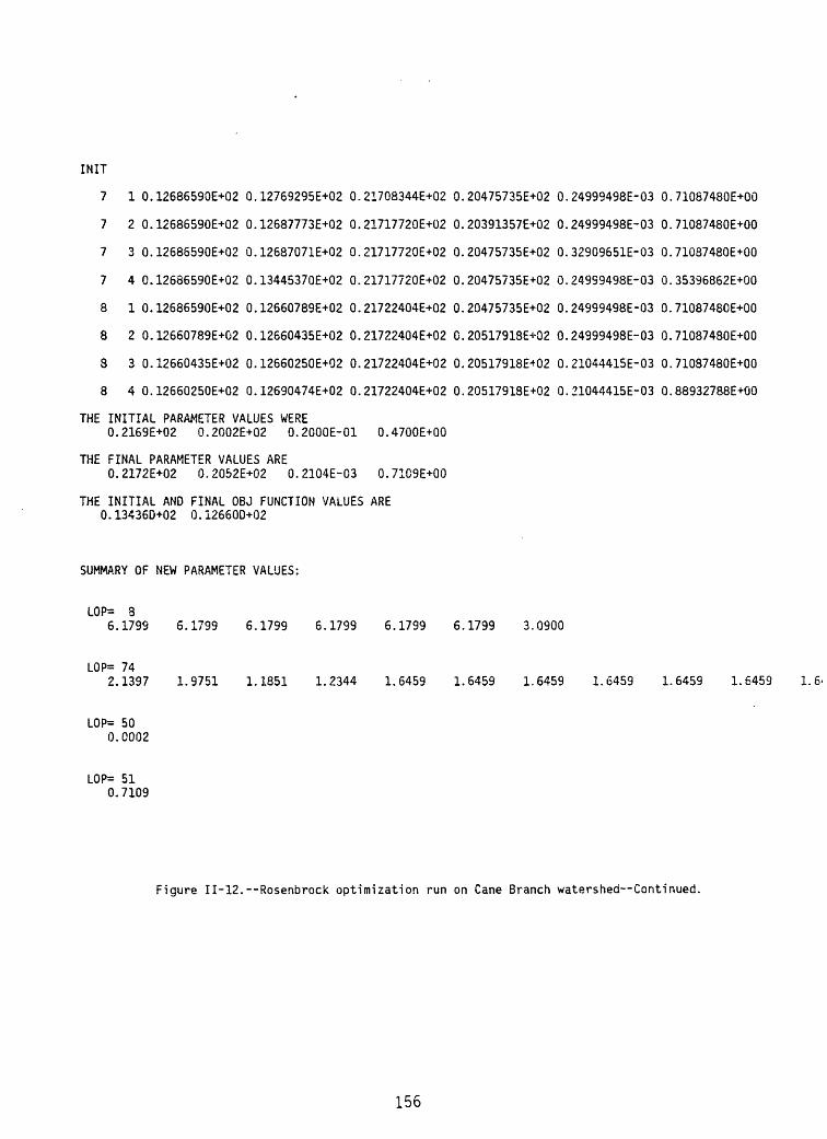
INIT
7 1 0.12686590E+02 0.12769295E+02 0.21708344E+02 0.20475735E+02 0.24999498E-03 0.71087480E+00
7 2 0.12686590E+02 0.12687773E+02 0.21717720E+02 0.20391357E+02 0.24999498E-03 0.71087480E+00
7 3 0.12686590E+02 0.12687071E+02 0.21717720E+02 0.20475735E+02 0.32909651E-03 0.71087480E+00
7 4 0.12686590E+02 0.13445370E+02 0.21717720E+02 0.20475735E+02 0.24999498E-03 0.35396862E+00
8 1 0.12686590E+02 0.12660789E+02 0.21722404E+02 0.20475735E+02 0.24999498E-03 0.71087480E+00
8 2 0.12660789E+G2 0.12660435E+02 0.21722404E+02 C.20517918E+02 0.24999498E-03 0.71087480E+00
8 3 0.12660435E+02 0.12660250E+Q2 0.21722404E+02 0.20517918E+02 0.21044415E-03 0.71087480E+00
8 4 0.12660250E+02 0.12690474E+02 0.21722404E+02 0.20517918E+02 0.21044415E-03 0.88932788E+00
THE INITIAL PARAMETER VALUES WERE0.2169E+02 0.2Q02E+02 0.2000E-01 0.4700E+00
THE FINAL PARAMETER VALUES ARE0.2172E+02 0.2052E+02 0.2104E-03 0.71C9E+00
THE INITIAL AND FINAL OBJ FUNCTION VALUES ARE 0.13436D+02 0.12660D+02
SUMMARY OF NEW PARAMETER VALUES:
LOP= 86.1799 6.1799 6.1799 6.1799 6.1799 6.1799 3.0900
LOP= 742.1397 1.9751 1.1851 1.2344 1.6459 1.6459 1.6459 1.6459 1.6459 1.6459 1.64
LOP= 50 0.0002
LOP= 51 0.7109
Figure 11-12.--Rosenbrock optimization run on Cane Branch watershed Continued.
156
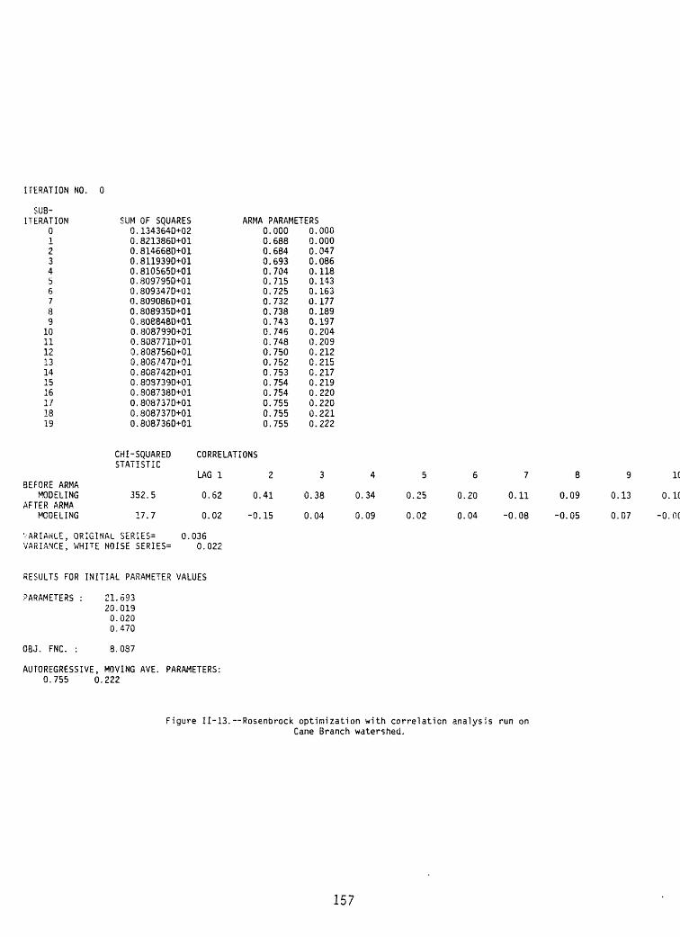
ITERATION NO. 0
SUB- ITERATION
0123456789
10111213141516171819
SUM OF SQUARES 0.134364D+02 0.821386D+01 0.814668D+01 0.8119390+01 0.810565D+01 0.809795D+01 0.809347D+01 0.809086D+01 0.808935D+01 0.808848D+01 0.8087990+01 0.808771D+01 0.8087560+01 0.808/470+01 0.808742D+01 0.80S739D+01 0.8087380+01 0.808737D+01 0.8087370+01 0.808736D+01
ARMA PARAMETERS0.000 0.0000.688 0.0000.684 0.0470.693 0.0860.704 0.1180.715 0.1430.725 0.1630.732 0.1770.738 0.1890.743 0.1970.745 0.2040.748 0.2090.750 0.2120.752 0.2150.753 0.2170.754 0.2190.754 0.2200.755 0.2200.755 0.2210.755 0.222
BEFORE ARMA MODELING
AFTER ARMA MODELING
CHI-SQUARED STATISTIC
352.5
17.7
CORRELATIONS
LAG 1 2
0.62 0.41
0.02 -0.15
VARIANCE, ORIGINAL SERIES= 0.036 VARIANCE, WHITE NOISE SERIES= 0.022
RESULTS FOR INITIAL PARAMETER VALUES
PARAMETERS
OBJ. FNC.
21.69320.0190.0200.470
8.087
AUTOREGRESSIVE, MOVING AVE. PARAMETERS: 0.755 0.222
3
0.38
0.04
4
0.34
0.09
5
0.25
0.02
6
0.20
0.04
7
0.11
-0.08
0.09
-0.05
9
0.13
O.D7
1C
0.1C
-O.OC
Figure 11-13.--Rosenbrock optimization with correlation analysis run on Cane Branch watershed.
157

ITERATION NO. 1
SUB- ITERATION
0123456789
10111213
SUM OF SQUARES 0.1375560+02 0.9705860+01 0.960905D+01 0.9573810+01 0.9559860+01 0.955434D+01 0.955221D+01 0.955141D+01 0.955112D+01 0.955101D+01 0.955097D+01 0.955095D+01 0.955095D+01 0.955095D+01
ARMA PARAMETERS0.000 0.0000.755 0.2220.756 0.2780.768 0.3230.779 0.3540.788 0.3750.794 0.3880.797 0.3960.800 0.4010.801 0.4030.802 0.4050.803 0.4060.803 0.4070.803 0.407
BEFORE ARMA MODELING
AFTER ARMA MODELING
CHI-SQUARED STATISTIC
222.1
13.1
CORRELATIONS
LAG 1
0.50
0.02
VARIANCE, ORIGINAL SERIES= 0.036 VARIANCE, WHITE NOISE SERIES= 0.026
RESULTS FOR ADJUSTMENT 1, PARAMETER 1
PARAMETERS
OBJ. FNC. :
OLD21.69320.0190.0200.470
3.087
NEW21.79320.0190.0200.470
9.551
AUTOREGRESSIVE, MOVING AVE. PARAMETERS: 0.803 0.407
2
0.33
-0.12
3
0.33
0.04
4
0.28
0.07
5
0.18
-0.02
6
0.13
-0.01
7
0.06
-0.06
8
0.04
-0.07
9
0.08
0.07
10
0.03
-0.03
Figure 11-13.--Rosenbrock optimization with correlation analysis run on Cane Branch watershed Continued.
158

THE INITIAL PARAMETER VALUES WERE0.2169E+02 0.2002E+02 0.2000E-01 0.4700E+00
THE FINAL PARAMETER VALUES ARE0.2171E+02 0.2069E+02 0.1215E-03 0.7109E+00
THE INITIAL AND FINAL OBJ FUNCTION VALUES ARE 0.808740+01 0.789780+01
SUMMARY OF NEW PARAMETER VALUES:
LOP= 86.0936 6.0936 6.0936 8.0936 6.0936 6.0936 3.0468
LOP= 742.5431 2.3474 1.4085 1.4671 1.9562 1.9562 1.9562 1.9562 1.9562 1.9562 1.9562 2.9343
LOP= 50 0.0001
LOP= 51 0.7109
AUTOREGRESSIVE, MOVING AVE. PARAMETERS: 0.776 0.281
Figure 11-13.--Rosenbrock optimization with correlation analysis run on Cane Branch watershed--Continued.
159
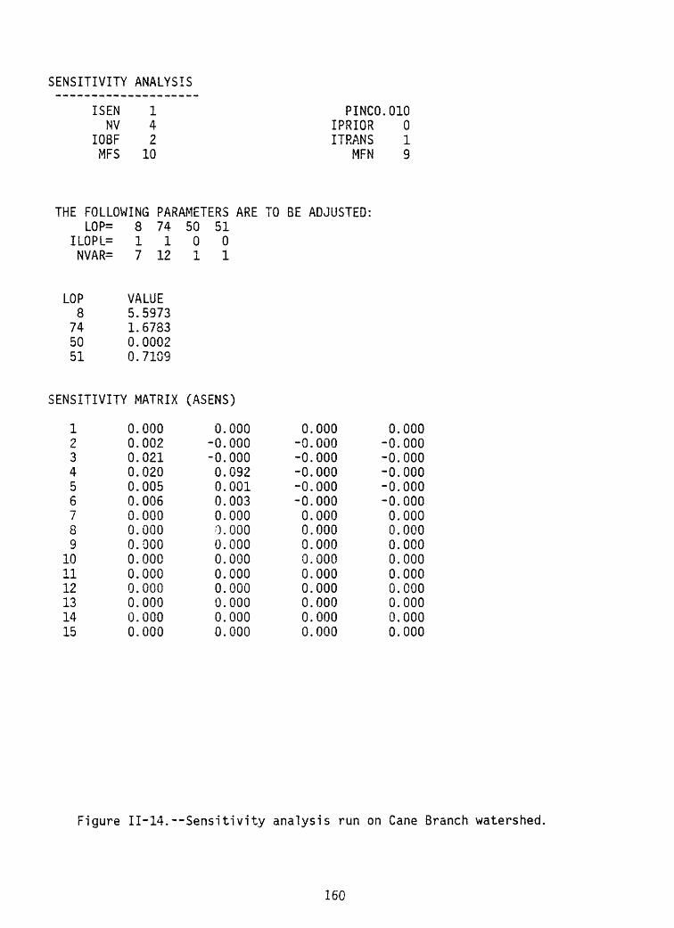
SENSITIVITY ANALYSIS
ISEN 1NV 4
IOBF 2NFS 10
PINC0.010IPRIOR 0ITRANS 1
MFN 9
THE FOLLOWING PARAMETERS ARELOP= 8 74 50 51
ILOPL= 1100NVAR= 7 12 1 1
"0 BE ADJUSTED:
LOP8
745051
VALUE5.59731.67830.00020.7109
SENSITIVITY MATRIX (ASENS)
123456789
101112131415
0.0000.0020.0210.0200.0050.0060.0000.0000.0000.0000.0000.0000.0000.0000.000
0.000-0.000-0.0000.0920.0010.0030.0000.0000.0000.0000.0000.0000.0000.0000.000
0.000-0.000-0.000-0.000-0.000-0.0000.0000.0000.0000.0000.0000.0000.0000.0000.000
0.000-0.000-0.000-0.000-0.000-0.0000.0000.0000.0000.0000.0000.0000.0000.0000.000
Figure 11-14. Sensitivity analysis run on Cane Branch watershed,
160

SENSITIVITY MATRIX (ASENS) Continued
16171319202122232425262728293031
i23456789
101112131415161718192021222324252627282930
0.0000.0040.0190.0000.0000.0340.0440.0000.0000.0000.0450.0000.0000.0000.000
-2.386
-0.219-0.218-0.218-0.217-0.217-0.217-0.216-0.2160.8800.457
-0.0940.2360.1390.0730.0060.153
-0.001-0,0010.1060.115
-0.0030.3990.025
-0.004-0.004-0.005-0.0050.5020.614
-0.005
0.0000.0010.0040.0000.0000.0050.1150.0000.0000.0000.0230.0000.0000.0000.0000.012
0.0010.0000.0010.0010.0010.0010.0010.001
-0.001-0.0000.0010.000
-0.000-0.000-0.000-0.0000.0000.000
-0.000-0.0000.000
-0.0000.0000.0000.0000.0000.000-0.0000.0990.000
0.0000.000
-0.0000.0000.000
-o.ooo-0.0000.0000.0000.000
-0.0000.0000.0000.0000.0000.003
-0.006-0.006-0.006-0.006-0.006-0.006-0.006-0.006-0.001-0.0010.0020.000-0.000-0.0000.000
-0.000-0.000-0.000-0.000-0.000-0.000-0.000-0.000-0.000-0.000-0.000-0.000-0.001-0.001-0.000
0.0000.000
-0.0000.0000.000
-0.000-0.0000.0000.0000.000
-0.0000.0000.0000.0000.0000.004
-0.221-0.221-0.222-0.222-0.223-0.223-0.224-0.224-0.015-0.004-0.026-0.012-0.000-0.000-0.000-0.000-0.001-0.001-0.001-0.002-0.003-0.002-0.003-0.004-0.004-0.004-0.004-0.002-0.002-0.005
OCTOBER
SEPTEMBER
Figure 11-14.--Sensitivity analysis run on Cane Branch watershed Continued,
161

INFORMATION MATRIX (ZINFC)
0.2500E-01 -0.5066E-04 -0.4489E-04 -0.7683E-04
-C.5066E-04 0.2667E-06 0.7054E-07
-0.2756E-06
-0.4489E-04 0.7054E-07 0.1674E-06 0.2058E-05
-0.7683E-04 -0.2756E-06 0.2058E-05 0.2139E-03
ERROR PROROGATION:TABLE OF MEAN SQUARED RUNOFF PREDICTION ERROR RESULTING FROM PARAMETER ERRORS
LOP
8745051
JOINT
MAGNITUDE OF PARAMETER ERROR 5% 10% 20%
0.001220.000000.000000.000010.00123
0.004890.000000.000000.000040.00493
0.019560.000000.000000.000170.01973
50%
0.122270.000000.000000.001050.12332
RESIDUALS ANALYSIS
VARIANCE STD DEV MEAN ABS
0.035070.187270.11180
PARAMETER
8745051
VALUE
5.59731.67830.00020.7109
STANDARD ERROR JOINT INDIVIDUAL
0.1375 0.0785 9,3196 7.2014 0.0018 0.0011 0.1204 0.1077
PARAMETER CORRELATION MATRIX (ZINV)
1.0000.5550.684
-0.255
0.5551.0000.155
-0.004
0.6840.1551.000
-0.441
-0.255-0.004-0.441 1.000
Figure 11-14.--Sensitivity analysis run on Cane Branch watershed Continued,
162

DIAGONAL ELEMENTS OF HAT MATRIX (PDENT)
0.0000.0000.0000.002
0.0060.0000.000
0.0000.0010.0560.014
0.0130.0730.0690.114
0.0140.0100.006
0.0050.0480.0060.003
0.0160.0090.004
0.0020.0010.0010.000
0.0000.0000.000
0.0000.0000.0000.000
0.0000.0000.0000.000
0.0000.0000.000
0.0000.0000.008
0.0020.0000.000
0.0000.0030.038
0.0120.0220.062
0.0860.0090.047
0.0040.0480.046
0.0020.0120.004
0.0020.0010.003
0.0000.0000.000
0.0000.0000.000
0.0000.0000.000
0.0000.0000.000
0.0000.0000.000
0.0010.0000.000
0.0000.0100.005
0.0110.0170.092
0.0370.0080.020
0.0030.023O.C05
0.0020.0120.004
0.0020.0010.000
0.0000.0000.000
0.0000.0000.000
0.0000.0000.000
0.0000.0000.000
0.0030.0000.000
0.0000.0000.000
0.0000.0510.123
0.0180.0160.016
0.0310.0080.014
0.0060.0140.004
0.0230.0120.003
0.0020.0010.000
0.0000.0000.000
0.0000.0000.000
0.0000.0000,000
0.0000.0000.000
0.0000.0000.000
0.0000.0000.000
0.0000.2960.051
0.0400.0150.026
0.0210.0050.012
0.0060.0110.005
0.0050.0100.003
0.0020.0010.000
0.0010.0000.000
0.0000.0000.000
0.0000.0000.000
0.0000.0000.000
0.0000.0000.001
0.0000.0000.000
0.0000.2180.032
0.0080.0130.028
0.0260.0050.014
0.0150.0090.004
0.0020.0090.003
0.0020.0010.000
0.0000.0000.000
0.0000.0000.000
0.0000.0000.000
0.0000.0000.000
0.0000.0000.000
0.0000.0000.000
0.0000.1340.025
0.0270.0120.026
0.0280.0070.035
0.0130.0080.003
0.0020.0080.003
0.0010.0010.000
0.0000.0000.000
0.0000.0000.000
0.0000.0000.000
0.0000.0000.000
0.0000.0000.000
0.0000.0000.000
0.0000.0930.013
0.0230.0100.125
0.0290.0060.058
0.0240.0070.003
0.0360.0070.002
0.0010.0010.000
0.0000.0000.000
0.0000.0000.000
0.0000.0000.000
0.0000.0000.000
0.0000.0000.000
0.0000.0000.000
0.0010.0740.019
0.0260.0090.011
0.0140.027
0.0240.0060.003
0.0970.0060.002
0.0010.0010.000
0.0000.0000.000
0.0000.0000.000
0.0000.0000.000
0.0000.0000.078
0.0000.0000.000
0.0000.0000.000
0.0000.1120.015
0.0330.0220.134
0.0080.061
0.0250.0060.003
0.0100.0050.002
0.0010.0010.000
0.0000.0000.000
0.0000,0000.000
0.0000.0000.000
0.0000.0000.000
Figure II-14. Sensitivity analysis on Cane Branch watershed Continued.
163

series. The initial parameter values, objective function value, and the ARMA parameters are then listed.
Iteration 1 presents the same output sequence as iteration 0, except that parameter 1 has now been adjusted. The new parameter value and the new objective function are shown. In this example, the increase in parameter 1 by 10 percent had a deleterious effect on the simulation which is evidenced by the increase in the objective function. For the next iteration parameter 1 will be returned to its original value and parameter 2 will be changed. This iteration sequence and iteration step output will be repeated until NV (number of variables) times NTRY (number of cycles through parameters) iterations are completed. These will be followed by a summary table of initial and final parameter and objective function values and a listing of the distributed parameter values in the same format as shown in figure 11-12.
The operational sequence for an optimization run begins with a complete simulation for the period designated using the initial parameter estimates. The results of this simulation are output in a form dependent on the choices selected on the 'Q7PRINT0P' card in card group 1. This is followed by the optimization output shown in figure 11-12. Then another complete model simulation is run using the new 'best fit 1 parameter values. The results of this simulation are output after the optimization tables in the same format as the initial simulation run.
The sensitivity analysis output is shown in figure 11-14. The first section lists the input values specified in card group 7 and is followed by the summary of parameter values fitted in the previous optimization. The next section 'is the sensitivity matrix which is n x p in size where n is the number of days or storm periods and p is the number of parameters. The values output are relative sensitivities. Only the 61 values for October and September are shown out of the total 365 daily values output. This is followed by the information matrix. The diagonal elements of this matrix are the sums of squares of the sensitivity matrix columns. The off diagonal elements are the cross products of the sensitivity matrix columns.
Parameter errors are expressed in the next three sections. The first is the error propogation table showing the increase in the mean squared runoff prediction error resulting from various size errors in each parameter. These are the increases that would occur in the variance value expressed in the residuals analysis shown next. The error and variance values shown are log values because ITRANS=1 was selected in card group 7. The residuals analysis is followed by a list of the parameter values with their joint and individual error values.
Parameter correlations are shown in the next output segment which is the parameter correlation matrix. This is followed by the diagonal elements of the hat matrix.
164

ATTACHMENT VIII
Instructions for obtaining a copy of PRMS
A copy of PRMS on magnetic tape (9 track, 1600 BPI) may be obtained by sending a magnetic tape along with a written request to:
U.S. Geological SurveyWater Resources Division, Surface Water BranchNational Center, Mail Stop 41512201 Sunrise Valley DriveReston, VA 22092
A listing only may also be obtained by writing to the same address.
Inquiry should be made to this address regarding the cost of a copy request. Prepayment of the costs of producing a magnetic tape copy or listing is required. Check or money order, in exact amount, should be made payable to the U.S. Geological Survey.
207
Gauss-Newton Optimization Example
A second optimization procedure that can be selected is the Gauss-Newton procedure. This option is selected by making the IOPT parameter on card 1 of card group 1 negative. Figure 11-15 shows the output for one iteration of a daily simulation run using the Gauss-Newton optimization with correlation analysis. Input parameter values and options are presented in a form identi cal to figure 11-11 and immediately precede the output shown in figure 11-15.
Unlike the Rosenbrock procedure, the Gauss-Newton procedure moves all parameters at once during an iteration step. The first item output in each iteration is the sensitivity matrix which is used in computing the direction and magnitude of movement for each parameter. This is followed by the subiteration table of the ARMA modeling procedure used in the error correla tion analysis. This table and the subsequent ARMA output are the same as that described in the preceding section. The first subiteration table uses the parameter values available at the beginning of the current major iteration. For iteration 1, these are the initial parameter estimates. The first ARMA procedure is followed by the information matrix, the initial correction vector, and the correction vector multiplier. A table of the old and new adjusted parameters is then output. Using these new parameters, a second ARMA fitting is conducted and the results printed. A final correction vector multiplier is then computed using the Box-Kanemasu interpolation modification (Beck and Arnold, 1977). The old parameter values and the new parameter values computed using the new correction vector are output. A final ARMA fitting is conducted and the results are printed.
The sequence of procedures described and the outputs shown are repeated for each NTRY iteration requested. After the last iteration a table of initial and final objective functions and parameter values are output along with a table of the distributed parameter values in the same format as shown in fiqure 11-12.
165

GAUSS-NEWTON OPTIMIZATION
IOPT -2 NTRY 8NV 4 IPRIOR 0
IOBF 2 ITRANS 1MFS 10 MFN 9
THE FOLLOWING PARAMETERS ARE TO BE ADJUSTED:
LOP= 8 74 50 51ILOPL= 1100NVAR= 7 12 1 1
OTHE LOWER CONSTRAINTS AREO.OOOOOOE+00 O.QOOOOOE+00 O.OOOOOOE+00 O.OOOOOOE+00
OTHE UPPER CONSTRAINTS ARE0.100000E+02 Q.200000E+01 0.100000E+01 Q.100000E+01
OTHE TRANSFORMED LOWER CONSTRAINTS AREO.OOOOOOE+00 O.OOOOOOE+00 O.OOOOOOE+00 O.OOOOOOE+00
OTHE TRANSFORMED UPPER CONSTRAINTS ARE0.223026E+02 0.206931E+02 0.100000E+01 0.100000E+01
OTHE STARTING PARAMETER VALUES ARE0.216927E+02 0.200195E+02 0.200000E-01 0.470000E+00
OTHE INITIAL STEP SIZE INCREMENTS ARE0.100000E+00 0.100000E+00 0.100000E+00 0.100000E+00
OTHE TRANSFORMED INITIAL STEP SIZE INCREMENTS ARE0.460984E-02 0.499513E-02 0.100000E+00 0.100000E+00
Figure 11-15.--One iteration of Gauss-Newton optimization with correlation analysis on Cane Branch watershed.
166

ITERATION NUMBER 1
SENSITIVITY MATRIX (ASENS)
123456789
10111213141516171819202122232425262728293031
123456789
10111213
0.0000.0330.4490.4410.1000.1380.0000.0000.0000.0000.0000.0000.0000.0000.0000.0000.0950.4140.0000.0000.7290.9360.0000.0000.0000.9600.0000.0000.0000.000
-44.871
-6.323-6.313-6.303-6.293-6.283-6.273-6.264-6.25520.33810.253-2.2845.9323.091
0.0000.000
-0.000-0.0000.000
-0.0000.0000.0000.0000.0000.0000.0000.0000.0000.0000.0000.000
-0.0000.0000.000
-o.ooo-0.0000.0000.0000.0000.0000.0000.0000.0000.0000.153
0.0190.0190.0190.0190.0190.0190.0190.019
-0.000-0.001-0.012-0.006-0.001
0.0000.0000.0000.0000.0000.0000.000
'0.0000.0000.0000.0000.0000.0000.0000.0000.0000.000
-o.ooo0.0000.000
-o.ooo-o.ooo-o.ooo-o.ooo-o.ooo-o.ooo/-o.ooo-o.ooc-o.ooo-o.ooo0.000
-0.095-0.095-0.095-0.095-0.095-0.095-0.095-0.096-0.005-0.001-0.012-O.C05-0.000
0.0000.000
-o.ooo-o.ooo0.000
-o.ooo0.0000.0000.0000.0000.0000.0000.0000.000O.OGO0.0000.000
-o.ooo0.0000.000
-o.ooo-o.oooo.coo0.0000.000-o.ooo0.000
-o.ooo0.0000.0000.000
-0.141-0.141-0.140-0.140-0.140-0.140-0.140-0.140-0.008-0.002-0.017-0.008-o.ooo
OCTOBER
SEPTEMBER
Figure 11-15.--One iteration of Gauss-Newton optimization with correlation analysis on Cane Branch watershed Continued.
167

SENSITIVITY MATRIX (ASENS)--Continued
14 1.632 -0.000 -0.000 -0.00015 0.134 0.000 -0.000 -0.00016 3.397 -0.000 -0.000 -0.00017 -0.025 0.000 -0.000 -0.00018 -0.037 0.000 -0.000 -0.00119 2.204 -0.000 -0.001 -0.00120 2.421 -0.000 -0.001 -0.00121 -0.076 0.000 -0.001 -0.00122 9.754 -0.001 -0.000 -0.00123 0.608 0.000 -0.001 -0.00224 -0.107 0.000 -0.001 -0.00225 -0.114 0.000 -0.002 -0.00226 -0.120 0.000 -0.002 -0.00227 -0.126 0.000 -0.002 -0.00228 21.765 -0.001 -0.001 -0.00129 26.286 -0.001 -0.000 -0.00030 -0.136 0.000 -0.002 -0.003
SUB- ITERATION SUM OF SQUARES ARMA PARAMETERS
0 0.134364D+02 0.000 0.0001 0.821386D+01 0.688 0.0002 0.8146680+01 0.684 0.0473 0.8119390+01 0.693 0.0864 0.8105650+01 0.704 0.1185 0.8097950+01 0.715 0.1436 0.809347D+01 , 0.725 0.1637 0.809086D+01 0.732 0.1778 0.808935D+01 0.738 0.1899 0.8088480+01 0.743 0.197
10 0.808799D+01 0.746 0.20411 0.808771D+01 0.748 0.20912 0.8087560+01 0.750 0.21213 0.808747D+01 0.752 0.21514 0.808742D+01 0.753 0.21715 0.808739D+01 0.754 0.21916 0.8087380+01 0.754 0.22017 0.8037370+01 0.755 0.22018 0.808737D+01 0.755 0.22119 0.8087360+01 0.755 0.222
Figure 11-15.--One iteration of Gauss-Newton optimization with correlation analysis on Cane Branch watershed Continued.
168

BEFORE ARMA MODELING
AFTER ARMA MODELING
CHI-SQUARED STATISTIC
352.5
17.7
CORRELATIONS
LAG 1 2
0.62 0.41
0.02 -0.15
VARIANCE, ORIGINAL SERIES= 0.036 VARIANCE, WHITE NOISE SERIES= 0.022
3
0.38
0.04
4
0.34
0.09
5
0.25
0.02
6
0.20
0.04
7
0.11
-0.08
8
0.09
-0.05
9
0.13
0.07
10
0.10
-0.00
INFORMATION MATRIX (ZINFC)
0.6983E+Q1-0.1803E-02-0.5094E-03 0.9923E-04
-0.1303E-02 0.3767E-04-0.2712E-06-0.1841E-04
-0.5094E-03-0.2712E-06 0.3320E-06 0.3652E-05
0.9923E-04-0.1341E-040.3652E-050.1241E-03
INITIAL CORRECTION VECTOR: -0.0588 12.1704 -0.5256
PARAMETER PARAMETER PARAMETER PARAMETER PARAMETER
OUTSIDE CONSTRAINTS, OUTSIDE CONSTRAINTS, OUTSIDE CONSTRAINTS, OUTSIDE CONSTRAINTS,
0.5898ALPHA HALVED, ALPHA HALVED, ALPHA HALVED, ALPHA HALVED,
ALP= ALP= ALP= ALP=
OUTSIDE CONSTRAINTS, ALPHA HALVED, ALP=
1.0000.5000.2500.1250.063
CORRECTION VECTOR MULTIPLIER: 0.031
PARAMETERSOLD
21.69320.0190.0200.470
NEW21.69120.4000.0040.488
SUB- ITERATION
0123
SUM OF SQUARES 0.133020D+02 0.804972D+01 0.804967D+01 0.8049660+01
ARMA PARAMETERS 0.000 0.000 0.755 0.222 0.754 0.222 0.754 0.222
Figure II-I5.--One iteration of Gauss-Newton optimization with correlation analysis on Cane Branch watershed Continued.
169

CHI-SQUARED STATISTIC
BEFORE ARMAMODELING
AFTER ARMAMODELING
345.
17.
5
4
CORRELATIONS '
LAG 1 2
0.61
0.02
0.41
-0.14
3
0.38
0.04
4
0.34
0.09
5
0.25
0.02
6
0.19
0.04
7
0.10
-0.08
8
0.09
-0.05
9
0.13
0.07
o.
VARIANCE, ORIGINAL SERIES= 0.036 VARIANCE, WHITE NOISE SERIES= 0.0.22
OBJ. FNC. 8.087 8.050
FINAL RESULTS FOR ITERATION 1 CORRECTION VECTOR MULTIPLIER:
PARAMETERS :OLD
21.69320.0190.0200.470
NEW21.69120.4380.0020.490
0.034
SUB- ITERATION
012
SUM OF SQUARES 0.132890D+02 0.804628D+01 0.804627D+01
ARMA PARAMETERS 0.000 0.000 0.754 0.222 0.753 0.222
BEFORE ARMAMODELING
AFTER ARMAMODELING
CHI-SQUARED STATISTIC
344.8
17.4
CORRELATIONS
LAG 1 2
0.61
0.02
0.41
-0.14
3
0.38
0.04
4
0.34
0.09
5
0.25
0.02
6
0.19
0.04
7
0.10
-0.08
8
'0.09
-0.05
9
0.12
0.07
0
0
VARIANCE, ORIGINAL SERIES= 0.036 VARIANCE, WHITE NOISE SERIES= 0.022
OBJ. FNC. 8.087 8.046
Figure 11-15. One iteration of Gauss-Newton optimization with correlation analysis on Cane Branch watershed Continued.
170

ATTACHMENT III
Procedure DCARDS
This procedure contains several subroutines that will read cards with different input formats and write records to online disk storage in the WATSTORE sequential format. The card formats that are currently available for input are: (1) WATSTORE standard daily- and unit-values input formats; (2) "Carter Card" format for daily and unit values; and (3) a variable daily format. Formats of the control cards and data cards are described below.
Input Format--WATSTORE Daily
This subroutine will read data in the U.S. Geological Survey WATSTORE standard daily values card format. Program control cards as shown below are inserted before and after data cards.
CARD
123
COLUMNS FORMAT
117-64 2-16
II12A43A4,A3
4-51
29-33
34-38
2-16
15
15
3A4,A3
17-20 21-22 23-24
25-80
141212
8F7.0
VARIABLE
ITYP TITL STAID
FARM
STAT
STAID
YEARIM0ICD
DATA(I)
Repeat cards 4-51 for each year.
52 II ICODE
DESCRIPTION
WATSTORE Daily=0Station name15-digit station identifi
cation numberWATSTORE 5-digit parameter
codeWATSTORE 5-digit statistic
code15-digit station identifi
cationWater year of recordMonthSequence number of card within month (ICD=1,2,3,4)
8 data values per card
8=end of parameter code orstatistic code
9=end of station
NOTE: For new parameter or statistic code, start at card 3. For new station,start at card 1.
Input Format--WATSTORE unit
1 II ITYP WATSTORE Unit=4 17-64 12A4 TITL Station name 2-16 3A4,A3 STAID 15-digit station identifi
cation number29-33 15 PARM WATSTORE 5-digit parameter
code
171

CARD
Input Format--WATSTORE Unit--Continued.
COLUMNS FORMAT VARIABLE DESCRIPTION
34-38 15 STAT
117-2021-2223-2425-2627-2829-3031-3539-80
Al141212121212156F7.0
FLAGLYRLMOLDYLHRLMNLSCRPDDATA(I)
Repeat card 4 as necessary
1 Al FLAG
3--(un1t data)
WATSTORE 5-digit statisticcode
B=unit values data Calendar year Month DayHour (1st observation) Minute SecondReadings per day Unit values for six consecutive
time intervals
"2"=new time interval,continue with card 4
"7"=new station,continue with card 2
"8!l =new parameter or statisticcode, continue with card 3
"9"=end of WATSTORE Unit valuescard
Input Format--Carter Cards
1 II ITYP Carter=l 9-56 12A4 T1TL Station name
59-64 F6.0 PTIME Time interval for unit data 65-79 3A4,A3 STAID 15-digit station identifi
cation 80 II IC0DE Unit sediment=0
Unit precipitation=l Unit discharge=2 Daily precipitation=3 Daily evaporation=4 Daily maximum temperature
(°C)=5 Daily minimum temperature
(°C)=6 Daily solar radiation=7
9-10 12 IYR Year
11-12 12 IM0 Month13-14 12 IDY Day17-18 12 ICD Card sequence number19-78 12F5.0 DATA(I) Unit data80 II IC0DE Same as card 2
172

CARD COLUMNS FORMAT VARIABLE DESCRIPTION
IYR3 (daily 9-10 12 data)
11-12 13
14-77 80
4 80
Repeat cards 2-4 for all records.
5 79X.I1 IC0DE
12 11 16F4.2 11 11
IM0 ICD DATA(I) IC0DE IC0DE
Year
MonthCard sequence (1 or 2)Daily dataSame as card 2'8' to signify end of record
'9 1 to signify end of Carter cards
Input Format Variable Daily
This option reads in daily data, one card per day with up to 8 variables per card. The format of the data cards is read in along with parameter and statistic codes corresponding to the variables.
CARD COLUMNS FORMAT DESCRIPTION
Variable format=215-digit station identifi
cationTitleNumber of variables read per
day (maximum=8)WATSTORE parameter code for
each data itemStatistic code for each data
itemFormat of data cards, in parentheses
Month of observationDayYearVariables up to 8 per card
Note: Place 99 in columns for 'IM0' at end of variable format data.
12
3
4
5
6--(One card per day)
1 2-16
17-64 65-66
1-40
1-40
1-80
1-2 3-4 5-8 S-80
11 3A4,A3
12A4 12
815
815
20A4
12 12 14 Variable
ITYPE STAID
TITL NV
PARM(I)
STAT(I)
F0RM(I)
IM0 IDY IYR DV(I)
173

The JCL and deck setup to run DCARDS is as follows
// J0B CARD //PR0CLIB DO DSN=DG4812S.PRDAT.LIB,DISP=SHR// EXEC DCARDS, UVAL=' useri d.ds name. DATA ' ,// DVAL=' user id. dsname. DATA'//SYS IN DD~*
program control cards and data
/*
Underlined items should be replaced with the data set name for the unit values (UVAL) and daily values (DVAL) sequential output files.
An example of WATSTORE card format for daily values and Carter card format for storm period values is shown in figure III-l. One water year of daily data for streamflow, precipitation, maximum and minimum air temperature and pan evaporation, in WATSTORE card format, and 45 storm days of streamflow and precipitation at 15-minute intervals in Carter card format were input to DCARDS. The resulting DCARDS output which indicates by water year and storm day the station identification, parameter code, and statistics code of each record created is shown in figure HI-2. DCARDS creates both a daily records file and a storm days file. These two output files were then used as input to program GENDISK to create a PRMS compatible ISAM file. The GENDISK output is shown in figure III-3.
174

//DG4812SD JOB (*********,DOOO),'SAINDON 1 ,CLASS=B //PROCLIB DO DSN=DG4812S.PRDAT.LIB.DISP=SHR // EXEC DCARDS,DVAL='DG4812S.TESTD.DATA', // UVAL='DG4812S.TESTU.DATA' //SYSIN DD *
02462500BLACK WARRIOR R AT BANKHEAD L&D NEAR BESSEMER AL024625000246250019761001024625001976100202462500197610030246250019761004
0246250019770901024625001977090202462500197709030246250019770904
024625000246250019761001024625001976100202462500197610030246250019761004
0246250019770901024625001977090202462500197709030246250019770904
02462500 0006000003 ENT02462500197610011960.00 590.00 890.00 530.002260.002770.002350.003760.0002462500197610022740.00 530.00 590.00 470.00 300.00 590.00 300.00 720.000246250019751003 530.00 530.00 590.00 410.002630.001500.00 410.00 470.000246250019761004 590.001570.00 770.00 840.001520.00 470.00 710.00
000200000123.9016.1024.4020.50
35.5031.7030.0029.40
27.8018.3018.3021.10
35.5031.1031.1028.90
30.23.20.15.
34.31.33.31.
00305060
40703070
30.25.20.13.
34.30.26.31.
00505090
40501070
000200000212.2010.0011.1015.00
20.5020.0020.5020.00
12.205.606.1010.00
19.4020.0019.4020.00
12.6.5.3.
18.19.18.15.
20700090
90409060
15.7.7.3.
22.15.17.20.
00202090
20608050
ENT30.5025.5011.7014.40
32.8031.7028.9030.00
ENT15.009.403.303.30
21.7016.1016.7019.40
30.26.17.13.
31.29.30.21.
19.10.4.3.
21.20.17.18.
CO702090
70405010
40004030
70502090
20.28.22.18.
25.31.29.
11.10.4.8.
22.20.15.
50302030
501040
10004030
205060
22.2027.2024.40
26.7030.0031.70
12.2010.008.30
20.5020.5018.30
02462500197709011500.001330.00 700.00 590.00 650.001590.00 10300. 15100.02462500197709025100.00 800.001340.002860.003700.004730.004940.004900.0002462500197709035200.00 710.005020.003990.003080.002760.002410.00 150.0002462500197709041680.009960.006940.007430.006190.00 10000.
Figure III-l.--Card deck used to run DCARDS procedure.
175
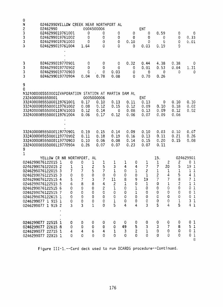
0 N 02462990YELLOW CREEK NEAR2 024629903 02462990197610013 02462990197610023 02452990197610033 0246299019761004
3 02462990197709013 02462990197709023 02462990197709033 0246299019770904
90N324000085550001EVAPORATION2324000085550001332400008555000119761001332400008555000119761002332400008555000119761003332400008555000119761004
33240000855500011977090133240000855500011977090233240000855500011977090333240000855500011977090491
NORTHPORT AL0004500006
000
1.64
000
0.04
0000
000
0.78
STATION AT
0000
00
0.030.08
MARTIN
0.
0.
DAM
00
100
32000
AL0005000006
0.170.080.120.06
0.190.110.100.26
YELLOW CR NR NORTHPORT,0246299076122015 1 00246299076122015 2 1024629S076122015 3 70246299076122515 3 00246299076122515 4 50246299076122515 5 60246299076122515 6 00246299076122515 7 00246299076122615 1 00246299077 1 915 1 00246299077 1 915 2 3
0246299077 22515 i 00246299077 22615 8 00246299077 22715 1 40246299077 22315 1 0
01707800003
0040
AL12503800001
0060
0.100.120.140.17
0.150.180.060.07
15707420000
0040
0.130.15
00.12
0.140.190.080.07
1310
11210015
0010
0.0.0.0.
0.0.0.0.
14008100004
04930
11120806
09161423
04109011004
0520
ENT000
0.03
0.440.01
00.70
ENT0.130.090.130.07
0.100.130.150.07
1721
191000C3
0310
0.
0.
4.0,
0.
0.0.0.
0.0.0.0.
15.17127
000005
0300
5900
19
38530
26
0100909
03112011
0000
0.380.64
0
0.100.180.120.08
0.100.210.15
00.330.01
01.31
0
0.100.020.02
0.070.260.08
0246299012
20147100004
0700
25158200015
0800
0 119 11 14 17 11 10 10 10 13 14 1
0 15 10 10 1
Figure III-l. Card deck used to run DCARDS procedure Continued.
176

YELLOW CR NR NORTHPORT, AL 15. 0246299020246299076122015 1 8.10 8.10 8.10 8.10 8.10 8.10 8.10 8.10 8.10 8.10 8.10 8.40 20246299076122015 2 8.40 8.40 8.40 8.40 8.80 8.80 9.10 9.10 9.50 9.90 10.0 11.0 20246299076122015 3 13.0 15.0 17.0 20.0 24.0 28.0 30.0 33.0 37.0 44.0 49.0 53.0 20246299076122015 4 56.0 60.0 61.0 62.0 52.0 62.0 62.0 61.0 60.0 61.0 60.0 58.0 20246299076122015 5 57.0 56.0 56.0 55.0 53.0 52.0 51.0 49.0 48.0 46.0 45.0 45.0 20246299076122015 6 43.0 42.0 40.0 39.0 38.0 36.0 35.0 35.0 34.0 32.0 32.0 31.0 20246299076122015 7 30.0 29,0 29.0 28.0 27.0 27.0 26.0 25.0 25.0 24.0 24.0 23.0 20246299076122015 8 23.0 23.0 22.0 22.0 21.0 21.0 21.0 21.0 21.0 20.0 20.0 20.0 20246299076122515 1 9.50 9.50 9.50 9.10 9.10 9.10 9.10 9.10 9.10 9.10 9.10 9.10 20246299076122515 2 9.10 9.10 9.10 9.10 9.10 9.10 9.10 9.10 9.10 9.10 9.10 9.10 20246299076122515 3 9.10 9.10 9.10 9.10 9.10 9.10 9.10 9.10 9.10 9.10 9.10 9.10 20246299076122515 4 9.10 9.50 9.50 9.50 9.90 10.0 10.0 11.0 11.0 12.0 13.0 15.0 20246299076122515 5 18.0 21.0 26.0 32.0 37.0 43.0 50.0 59.0 68.0 76.0 83.0 85.0 20246299076122515 6 88.0 90.0 90.0 91.0 88.0 87.0 87.0 85.0 84.0 82.0 81.0 79.0 20246299076122515 7 77.0 76.0 75.0 74.0 73.0 72.0 71.0 69.0 67.0 67.0 65.0 64.0 20246299076122515 8 62.0 61.0 59.0 58.0 56.0 54.0 52.0 51.0 49.0 47.0 46.0 44.0 20246299076122615 1 44.0 43.0 42.0 41.0 40.0 39.0 38.0 37.0 37.0 36.0 35.0 35.0 20246299076122615 2 35.0 34.0 33.0 32.0 32.0 32.0 32.0 31.0 31.0 30.0 30.0 30.0 20246299076122615 3 30.0 29.0 29.0 28.0 28.0 28.0 28.0 28.0 28.0 27.0 27.0 27.0 20246299076122615 4 26.0 26.0 25.0 25.0 25.0 25.0 25.0 25.0 24.0 24.0 24.0 23.0 20246299076122615 5 23.0 23.0 23.0 23.0 23.0 23.0 23.0 23.0 22.0 22.0 22.0 22.0 20246299076122615 6 21.0 21.0 21.0 21.0 21.0 21.0 21.0 21.0 21.0 21.0 21.0 20.0 20246299076122615 7 20.0 20.0 20.0 20.0 20.0 20.0 20.0 20.0 20.0 20.0 19.0 19.0 20246299076122615 8 19.0 19.0 19.0 19.0 19.0 19.0 19.0 19.0 19.0 19.0 19.0 19.0 20246299077 1 915 1 11.0 11.0 11.0 11.0 11.0 11.0 11.0 11.0 11.0 11.0 11.0 11.0 20246299077 1 915 2 11.0 11.0 11.0 11.0 11.0 11.0 11.0 11.0 11.0 11.0 11.0 15.0 2
0246299077 22515 1 24.0 24.0 24.0 24.0 24.0 23.0 23.0 23.0 23.0 23.0 23.0 23.0 20246299077 22515 2 23.0 23.0 22.0 22.0 22.0 22.0 21.0 21.0 21.0 21.0 21.0 21.0 20246299077 22515 3 21.0 21.0 21.0 21.0 21.0 21.0 21.0 21.0 21.0 21.0 21.0 21.0 20246299077 22515 4 21.0 21.0 20.0 20.0 21.0 20.0 20.0 20.0 20.0 20.0 20.0 20.0 20246299077 22515 5 20.0 20.0 20.0 20.0 20.0 20.0 20.0 20.0 19.0 19.0 19.0 19.0 20246299077 22515 6 19.0 19.0 19.0 19.0 19.0 19.0 19.0 19.0 19.0 19.0 18.0 18.0 2
Figure III-l.--Card deck used to run DCARDS procedure Continued.
177

0246299077 22515 7 18.0 18.0 18.0 18.0 18.0 18.0 18.0 18.0 18.0 18.0 18.0 18.0 2 0246299077 22515 8 18.0 18.0 18.0 18.0 18.0 18.0 18.0 18.0 18.0 18.0 17.0 17.0 2 0246299077 22615 1 17.0 17.0 17.0 17.0 17.0 17.0 17.0 17.0 17.0 17.0 17.0 17.0 2 0246299077 22615 2 17.0 17.0 17.0 17.0 17.0 17.0 17.0 17.0 17.0 17.0 17.0 17.0 2 0246299077 22615 3 17.0 17.0 17.0 17.0 17.0 17.0 17.0 17.0 17.0 17.0 17.0 17.0 2 0246299077 22615 4 17.0 17.0 17.0 17.0 17.0 16.0 16.0 16.0 16.0 16.0 16.0 16.0 2 0246299077 22615 5 16.0 16.0 16.0 16.0 16.0 16.0 16.0 16.0 16.0 16.0 16.0 16.0 2 0246299077 22615 6 16.0 16.0 16.0 15.0 15.0 16.0 15.0 15.0 15.0 15.0 15.0 15.0 2 0246299077 22615 7 15.0 15.0 15.0 15.0 15.0 15.0 15.0 15.0 15.0 15.0 15.0 15.0 2 0246299077 22615 8 15.0 15.0 15.0 18.0 17.0 18.0 18.0 20.0 23.0 25.0 27.0 30.0 2 0246299077 22715 1 32.0 36.0 40.0 45.0 49.0 52.0 54.0 56.0 56.0 57.0 59.0 60.0 2 0246299077 22715 2 60.0 61.0 61.0 59.0 59.0 58.0 57.0 56.0 55.0 54.0 53.0 52.0 2 0246299077 22715 3 50.0 49.0 48.0 46.0 45.0 45.0 43.0 42.0 41.0 39.0 38.0 38.0 2 0246299077 22715 4 37.0 36.0 35.0 35.0 34.0 34.0 33.0 32.0 32.0 32.0 31.0 31.0 2 0246299077 22715 5 30.0 30.0 30.0 29.0 29.0 29.0 28.0 28.0 28.0 28.0 27.0 27.0 2 0246299077 22715 6 27.0 27.0 26.0 26.0 26.0 25.0 25.0 25.0 25.0 25.0 25.0 25.0 2 0246299077 22715 7 25.0 25.0 25.0 24.0 24.0 24.0 24.0 24.0 24.0 23.0 23.0 23.0 2 0246299077 22715 8 23.0 23.0 23.0 23.0 23.0 23.0 23.0 23.0 22.0 22.0 22.0 22.0 2 0246299077 22815 10000000000002
9 0 /*
Figure III-l.--Card deck used to run DCARDS procedure Continued.
178
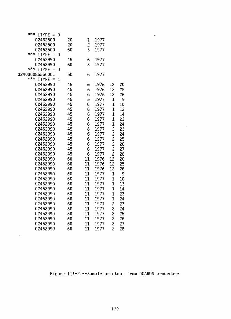
*** ITYPE = 002462500 20 1 197702462500 20 2 197702462500 60 3 1977
*** ITYPE = 002462990 45 6 197702462990 60 3 1977
*** ITYPE = 0324000085550001 50 6 1977
*** ITYPE = 102462990 45 6 1976 12 2002462990 45 6 1976 12 2502462990 45 6 1976 12 2602462990 45 6 1977 1 902462990 45 6 1977 1 1002462990 45 6 1977 1 1302462990 45 6 1977 1 1402462990 45 6 1977 1 2302462990 45 6 1977 1 2402462990 45 6 1977 2 2302462990 45 6 1977 2 2402462990 45 6 1977 2 2502462990 45 6 1977 2 2602462990 45 6 1977 2 2702462990 45 6 1977 2 2802462990 60 11 1976 12 2002462990 60 11 1976 12 2502462990 60 11 1976 12 2602462990 60 11 1977 1 902462990 60 11 1977 1 1002462990 60 11 1977 1 1302462990 60 11 1977 1 1402462990 60 11 1977 1 2302462990 60 11 1977 1 2402462990 60 11 1977 2 2302462990 60 11 1977 2 2402462990 60 11 1977 2 2502462990 60 11 1977 2 2602462990 60 11 1977 2 2702462990 60 11 1977 2 28
Figure III-2.--Sample printout from DCARDS procedure,
179
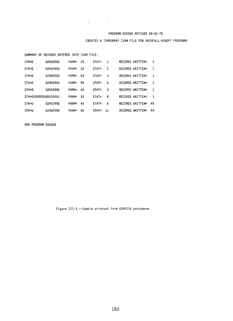
PROGRAM DSK268 REVISED 04-01-75
CREATES A TEMPORARY ISAM FILE FOR RAINFALL-RUNOFF PROGRAMS
SUMMARY OF RECORDS ENTERED INTO ISAM FILE:
STA=D 02462500
STA=0 02462500
STA=D 02462500
STA=D 02462990
STA=D 02462990
STA=0324000085550001
STA=U 02462990
STA=U 02462990
PARM=
PARM=
PARM=
PARM=
PARM=
PARM=
PARM=
PARM=
20
20
60
45
60
50
45
60
STAT=
STAT=
STAT=
STAT=
STAT=
STAT=
STAT=
STAT=
1
2
3
6
3
6
6
11
RECORDS
RECORDS
RECORDS
RECORDS
RECORDS
RECORDS
RECORDS
RECORDS
WRITTEN=
WRITTEN^
WRITTEN=
WRITTEN=
WRITTEN=
WRITTEN=
WRITTEN=
WRITTEN=
1
1
1
1
1
1
45
45
END PROGRAM DSK268
Figure III-3.--Sample printout from GENOI5K procedure.
180

ATTACHMENT IV
Definitions of System Variables
Definitions are listed alphabetically in table IV-1 for all input and common variables used in PRMS. Dimensions and labeled common areas are also indicated in the table.
ATTACHMENT V
Instructions for obtaining MAIN and subroutine listings
To obtain a listing of main and all Fortran subroutines, submit the following job (approximately 5,000 lines of print):
// J0B CARD // EXEC PGM=PDSLIST,PARM='LIST,INDEX,SPACE'//STEPLIB DD DSN=SYS1.USERLIB ) DISP=SHR//SYSPRINT DD SYS0UT=A//SYSUT9 DD DSN=DG4812S.PRMS83.F0RT,DISP=SHR//SYSIN DD DUMMY/*//
The following job can be run to obtain listings of selected subroutines:
// J0B CARD // EXEC PGM=PDSLIST,PARM='ALPHA,LIST,SPACE 1//STEPLIB DD DSN=SYS1.USERLIB,DISP=SHR//SYSPRINT DD SYS0UT=A//SYSUT9 DD DSN=DG4812S.PRMS83.F0RT,DISP=SHR//SYSIN DD *PRMAIN8ASFLW }I selected subroutine names
/*//
181

Table IM-I, Definitions of system variables
VARIABLE DIMENSION COMMON DESCRIPTION
AA
MODEAAI
AETAJMXALBALPIA
ALPHAALPRA
ALPR1AANSWARC
ARS
ASENSBAS
BASQ
BDYBDYIN
BDYOP
BMOBMOIN
BMOOP
BMSA
BPKBROBST
BWYBYLBYRBYRIN
BYROP
B4
11,100
11,50
50125050
50100
100 50
50
366,20
50
----
--
50
5050--
-- --
INITCD INITIAL AREA VALUE FOR EACH X-SECTION FOR EACHOVERLAND FLOW AND CHANNEL SEGMENT(SQ FT) - STORM
INITCD INITIAL AREA VALUES FOR EACH X-SECTION FORIMPERVIOUS AREA OF EACH OVERLAND FLOW PLANE(SQ FT)- STORM MODE
SM COMPUTED ACTUAL EVAPOTRANSPRIATION (INCHES)DPR RAIN/SNOW MIXTURE ADJUSTMENT COEFFICIENT, BY MONTHSNO COMPUTED ALBEDO FOR EACH HRUPCRCHA COEFFICIENT IN KINEMATIC ROUTING EQUATION FOR
IMPERVIOUS AREA OF EACH OVERLAND FLOW PLANE - STORMMODE
PCRCHA INVERSE OF ALPIA - STORM MODEPCRCHA COEFFICIENT IN KINEMATIC ROUTING EQUATION FOR
PERVIOUS AREA OF EACH OVERLAND FLOW PLANE ANDCHANNEL SEGMENTS - STORM MODE
PCRCHA INVERSE OF ALPRA - STORM MODESNO NOT CURRENTLY USEDBS CONTRIBUTING AREA ASSOCIATED WITH SPECIFIC GROUND
WATER RESERVOIR(ACRES)BS CONTRIBUTING AREA ASSOCIATED WITH SPECIFIC
SUBSURFACE RESERVOIR(ACRES)SENT1 SENSITIVITY MATRIX - SENSITIVITY ANALYSISBS TOTAL DAILY FLOW FROM ALL GROUNDWATER
RESERVOIRS(ACRE-INCHES)BS DAILY FLOW FROM EACH GROUNDWATER RESERVOIR
(ACRE- INCHES)DATES BEGIN DAY OF SIMULATIONDATOP BEGIN DAY OF INITIALIZATION PERIOD FOR
OPTIMIZATION OR SENSITIVITY ANALYSISDATOP BEGIN DAY OF OPTIMIZATION OR SENSITIVITY
ANALYSISDATES BEGIN MONTH OF SIMULATIONDATOP BEGIN MONTH OF INITIALIZATION PERIOD FOR
OPTIMIZATION OR SENSITIVITY ANALYSISDATOP BEGIN MONTH OF OPTIMIZATION OR SENSITIVITY
ANALYSISDSM MOISTURE STORAGE IN RECHARGE ZONE OF SOIL PROFILE
(INCHES) - STORM MODEVOL COMPUTED PEAK FLOW FOR EACH STORM PERIOD(CFS)VOL COMPUTED RUNOFF VOLUME FROM EACH STORM PERIOD(INCHES)DPR TEMPERATURE BELOW WHICH PRECIPITATION IS SNOW
AND ABOVE WHICH IT IS RAIN (DEGREES F OR C)SIZE BEGIN WATER YEAR FOR SIMULATIONALL NOT CURRENTLY USEDDATES BEGIN CALENDAR YEAR FOR SIMULATIONDATOP BEGIN YEAR OF INITIALIZATION PERIOD FOR
OPTIMIZATION OR SENSITIVITY ANALYSISDATOP BEGIN YEAR OF OPTIMIZATION OR SENSITIVITY
ANALYSIS OBJECTIVE FUNCTION SWITCH (-1.0=MINIMIZE)
182

Table IV-1. Definitions of system variables Continued
VARIABLE DIMENSION COMMON DESCRIPTION
CECN
CD
CDA
CMIA
CMI1ACMPA
CMP1ACOVDNS
COVDNW
CSELCTS
CTW
CTX
CX
C15
C24
C5
DARIPDARPDARUDATDATIPDATPDENDENI
DENMX
DFH
DIAG
12
50
50
50100
10050
50
--12
--
50
20
10,10
10,10
10,10
505050# --50
--
20
20
SNOP CONVECTION-CONDENSATION ENERGY COEFFICIENT FORMONTHS 1-12 (CAL/DEGREE ABOVE OC)
STORM DATA AVAILABILITY CODE (1=PRECIPITATION;2=1+DISCHARGE; 3=2+SEDIMENT) - STORM MODE
UNSS CUMULATIVE DRAINAGE AREA FOR EACH CHANNEL SEGMENT(ACRES) - STORM MODE
PCRCHA EXPONENT IN KINEMATIC ROUTING EQUATION FOR IMPERVIOUSAREA OF EACH OVERLAND FLOW PLANE - STORM MODE
PCRCHA INVERSE OF CMIA - STORM MODEPCRCHA EXPONENT IN KINEMATIC ROUTING EQUATIONS FOR
PERVIOUS AREA OF EACH OVERLAND FLOW PLANE ANDCHANNEL SEGMENTS - STORM MODE
PCRCHA INVERSE OF CMPA - STORM MODEDPR SUMMER COVER DENSITY FOR MAJOR VEGETATION
FOR EACH HRU (DECIMAL PERCENT)DPR WINTER COVER DENSITY FOR MAJOR VEGETATION
FOR EACH HRU (DECIMAL PERCENT)WX CLIMATE STATION ELEVATION(FT ABOVE MSL)ET AIR TEMPERATURE COEFFICIENT FOR ET COMPUTATION
FOR MONTHS 1-12ET COEFFICIENT FOR COMPUTING SNOWPACK SUBLIMATION FROM
PETET AIR TEMPERATURE COEFFICIENT FOR ET COMPUTATION
FOR EACH HRUSENT1 INITIAL PARAMETER VALUES IN OPTIMIZATION AND
SENSITIVITY ANALYSISSTOR Y INTERCEPT OF LINE DRAWN BETWEEN TWO ADJACENT
POINTS IN THE PULS ROUTING TABLE FOR 15 MINUTERESERVOIR ROUTING - STORM MODE
STOR Y INTERCEPT OF LINE DRAWN BETWEEN TWO ADJACENTPOINTS IN THE PULS ROUTING TABLE FOR 24 HOURRESERVOIR ROUTING
STOR Y INTERCEPT OF LINE DRAWN BETWEEN TWO ADJACENTPOINTS IN THE PULS ROUTING TABLE FOR 5 MINUTERESERVOIR ROUTING - STORM MODE
IMPRV IMPERVIOUS DRAINAGE AREA FOR EACH HRU (ACRES)IMPRV PERVIOUS DRAINAGE AREA FOR EACH HRU (ACRES)ALL DRAINAGE AREA OF EACH HRU (ACRES)ALL TOTAL BASIN DRAINAGE AREA (ACRES)IMPRV TOTAL IMPERVIOUS DRAINAGE AREA (ACRES)IMPRV TOTAL PERVIOUS DRAINAGE AREA (ACRES)SNO DENSITY OF SNOWPACK ON EACH HRUSNO INITIAL DENSITY OF NEW-FALLEN SNOW (DECIMAL
PERCENT)SNO AVERAGE MAXIMUM DENSITY OF SNOW PACK (DECIMAL
PERCENT)DFHSEG BEGAN AND END TIMES FOR EACH HYDROGRAPH SEGMENT
WITHIN SPECIFIED DAY - STORM MODESENT2 SQUARE ROOT OF DIAGONAL ELEMENTS OF INFORMATION
MATRIX-OPTIMIZATION AND SENSITIVITY ANALYSIS
183

Table IV-1. Definitions of system variables Continued
VARIABLE DIMENSION COMMON DESCRIPTION
DIN1
DIRLDPTDRAD
DRCOR
DRN
DS
DSCOR
DTDXA
DTDXMA
DTM
DTMA
DTMNDTOS
DTOSA
DTSA
DUM1DUM2DVP
DXA
DXDTA
DYLD50D50AEAIREDYEDYIN
EDYOP
ELCR
ELV
10
--50
50
366,7
50
100
100
100
100
100
366,5
100
100
50-_50
50
STOR SURFACE WATER RESERVOIR INFLOW FROM THE PREVIOUSTIME STEP (CFS)
ALL NOT CURRENTLY USEDOPSHO DEPTH OF SNQWPACK ON EACH HRU (INCHES) DAILY POTENTIAL SOLAR RADIATION FOR SLOPE-ASPECT
COMBINATION OF AN HRU (LANGLEYS)DPR DAILY PRECIPITATION CORRECTION FACTOR FOR RAIN
FOR EACH HRU DRAINAGE FACTOR FOR REDISTRIBUTION OF SATURATED
MOISTURE STORAGE AS A FRACTION OF KSATDVDT DAILY CLIMATE DATA FOR ONE YEAR AND UP TO 7
VARIABLE TYPESDPR DAILY PRECIPITATION CORRECTION FACTOR FOR SNOW
FOR EACH HRUPCRCHA OT/DX FOR EACH OVERLAND FLOW AND CHANNEL ROUTING
SEGMENT (SEC/FT) - STORM MODEPCRCHA (DT/DX) * CMA FOR EACH OVERLAND FLOW AND
CHANNEL ROUTING SEGMENT - STORM MODE ROUTING TIME INTERVAL FOR OVERLAND FLOW OR
CHANNEL SEGMENT (MINUTES) - STORM MODEPCRCHA ROUTING TIME INTERVAL FOR EACH OVERLAND FLOW AND
CHANNEL SEGMENT (MINUTES) - STORM MODEDTMN1 OUTPUT SWITCH - STORM MODE
-- PRINT OR PLOT OUTPUT TIME INTERVAL FOR 'OVERLANDFLOW OR CHANNEL SEGMENT (MINUTES) - STORM MODE
PCRCHA PRINT OR PLOT INTERVAL FOR EACH OVERLAND FLOWAND CHANNEL ROUTING SEGMENT (MINUTES) - STORM MODE
PCRCHA ROUTING TIME IN SECONDS FOR EACH OVERLAND FLOWAND CHANNEL SEGMENT - STORM MODE
DUMV USER DEFINED INPUT CLIMATE VARIABLE.DUMV USER DEFINED INPUT CLIMATE VARIABLE.DVDT DAILY OBSERVED PRECIPITATION FOR ONE YEAR AND UP
TO 5 GAGES (INCHES).PCRCHA LENGTH/NDX FOR EACH OVERLAND FLOW AND CHANNEL
SEGMENT - STORM MODEPCRCHA DX/DT FOR EACH OVERLAND FLOW AND CHANNEL ROUTING
SEGMENT (FT/SEC)ET POSSIBLE HOURS OF SUNSHINE, IN UNITS OF 12 HOURS NOT CURRENTLY USED
PCRCHA NOT CURRENTLY USEDSNO EMISSIVITY OF AIR ON DAYS WITHOUT PRECIPITATIONDATES END DAY OF SIMULATIONDATOP END DAY OF INITIALIZATION PERIOD FOR
OPTIMIZATION AND SENSITIVITY ANALYSISDATOP END DAY OF OPTIMIZATION OR SENSITIVITY
ANALYSIS- ELEVATION DIFFERENCE FROM CLIMATE STATION TO HRU
(THOUSANDS OF FEET)WX ELEVATION OF HRU (FEET ABOVE MSL)
184

Table IV-1.--Definitions of system variaJbles-'Continuedjf
VARIABLE DIMENSION COMMON DESCRIPTION
EMO DATES END MONTH OF SIMULATIONEMOIN DATOP END MONTH OF INITIALIZATION PERIOD FOR
OPTIMIZATION AND SENSITIVITY ANALYSIS EMOOP DATOP END MONTH OF OPTIMIZATION OR SENSITIVITY
ANALYSIS EN SEDIMENT PARAMETER FOR OVERLAND FLOW PLANE - STORM
MODEENA 50 PCRCHA EN FOR EACH OVERLAND FLOW PLANE - STORM MODE ENFIL 50 SM PRECIPITATION AVAILABLE FOR INFILTRATION ON
EACH HRU (INCHES)EPAN ET DAILY INPUT VALUE FOR PAN EVAPORATION (INCHES) EVC 12 ET EVAPORATION PAN COEFFICIENT FOR MONTHS 1-12 EVCAN MAXIMUM POTENTIAL DAILY INTERCEPTION LOSS (INCHES) EVIMP 50 IMPRV EVAPORATION LOSS FROM IMPERVIOUS AREA FOR EACH
HRU (INCHES)EWY SIZE END WATER YEAR FOR SIMULATION EXCS 50 SM DAILY SOIL WATER IN EXCESS OF SOIL MOISTURE
CAPACITY (SMAX) FOR EACH HRU (INCHES) EXSS 50 BS DAILY ACCUMULATED VOLUME OF WATER ADDED TO
A SUBSURFACE RESERVOIR (ACRE-INCHES)EYR DATES END CALENDAR YEAR FOR SIMULATION EYRIN DATOP END YEAR OF INITIALIZATION PERIOD FOR
OPTIMIZATION AND SENSITIVITY ANALYSIS EYROP DATOP END YEAR OF OPTIMIZATION OR SENSITIVITY
ANALYSIS FLGTH LENGTH OF OVERLAND FLOW PLANE OR CHANNEL SEGMENT
(FEET) - STORM MODEFREWT 50 SNO FREE WATER CONTENT OF SNOW ON EACH HRU (INCHES) FRN ROUGHNESS PARAMETER FOR OVERLAND FLOW PLANE OR
CHANNEL SEGMENT - STORM MODE FWCAP SNO FREE WATER HOLDING CAPACITY OF SNOWPACK
(DECIMAL PERCENT OF SNOWPACK WATER EQUIVALENT)G 60 SENT1 LOWER CONSTRAINT FOR EACH PARAMETER FOR OPTIMIZATION GSNK 50 BS COEFFICIENT TO COMPUTE SEEPAGE FROM EACH
GROUND-WATER RESERVOIR TO A GROUND-WATER SINKGU LOWER CONSTRAINT OF PARAMETER FOR OPTIMIZATION GW 50 BS STORAGE IN EACH GROUND-WATER RESERVOIR (ACRE-
INCHES)GWE1 DATOP NOT CURRENTLY USED GWE2 DATOP NOT CURRENTLY USEDGWS BS DAILY INFLOW TO ALL GROUND-WATER RESERVOIRS (INCHES) GWSNK 50 BS TOTAL SEEPAGE TO GROUND WATER SINK FOR EACH
GROUND-WATER RESERVOIR (ACRE-INCHES)H 60 SENT1 UPPER CONSTRAINT FOR EACH PARAMETER FOR OPTIMIZATION HA 1440 UNITRF ROUTED OUTFLOW FOR OVERLAND FLOW OR CHANNEL SEGMENTS
FOR 1-60 MINUTE INTERVALS - STORM MODE HC ~ SEDIMENT PARAMETER FOR OVERLAND FLOW PLANE - STORM
MODE
185

Table IV-1. Definitions of system variables Continued
VARIABLE DIMENSION COMMON DESCRIPTION
HCA 50 PCRCHA HC FOR EACH HRU - STORM MODEHORAB ALL POTENTIAL SHORTWAVE RADIATION ON HORIZONTAL SURFACE
FOR GIVEN DATE (LANGLEYS)HU UPPER CONSTRAINT OF PARAMETER FOR OPTIMIZATION ICBC EXC CHANGE PARAMETER VALUES SWITCH (0 = NO CHANGES
MADE TO PARAMETER VALUES DURING RUN; 1 = CHANGESMADE)
ICHG VOL COMPUTATION MODE SWITCH (0 = STORM COMPUTATIONS;1 = DAILY COMPUTATION)
ICOV 50 SM VEGETATION COVER TYPE FOR EACH HRU (0= BARE,1= GRASSES, 2= SHURBS, 3= TREES)
IC1 NOT CURRENTLY USED IC2 PEAK AND VOLUME SWITCH (0 = VALUES
COMPUTED FROM OBSERVED DISCHARGE; 1 = VALUESSUPPLIED BY USER) - STORM MODE
IDB DATES BEGIN DAY OF MONTH IDE DATES END DAY OF MONTH IDOUT OPT STORE PREDICTED DAILY VALUES SWITCH (0= NO
STORAGE; 1,2 = STORAGE FORMAT OPTIONS) IDPLB PLOT BEGIN DAY FOR DAILY PLOTS IDPLE PLOT END DAY FOR DAILY PLOTS IDS SIZE IND.EX FOR SPECIFIC RAIN GAGE DATA SET IDSW DISTRIBUTED PARAMETER ADJUSTMENT SWITCH FOR
OPTIMIZATION OR SENSITIVITY ANALYSIS (0 = ADJUSTALL PARAMETERS; 1 = ADJUST SELECTED PARAMETERS)
IDUM -- SIZE DUMMY VARIABLE IDUS 10 SIZE DATA USE SWITCH FOR DATA TYPES 1-10 (0= NOT USED;
1= USED)IDY SIZE CURRENT DAY OF MONTH COUNTER IGOPT DATOP NOT CURRENTLY USED IHS NUMBER OF HYDROGRAPH SEGMENTS IN A STORM PERIOD -
STORM MODE ILOPL 100 SENT1 DISTRIBUTED PARAMETER ADJUSTMENT SWITCH FOR
OPTIMIZATION AND SENSITIVITY ANALYSIS (0= EQUALINCREMENTS; 1=PROPORTIONAL INCREMENTS)
IMO SIZE CURRENT MONTH COUNTERIMPERV 50 UPR PERCENT IMPERVIOUS AREA FOR EACH HRU (DECIMAL) IMPLB PLOT BEGIN MONTH FOR DAILY PLOTS IMPLE PLOT END MONTH FOR DAILY PLOTS INIT OPT INITIALIZATION SWITCH - OPTIMIZATION AND
SENSITIVITY ANALYSIS INPR 50 DPR JULIAN DATES FOR ADJUSTING SNOWPACK WATER
EQUIVALENTS FOR EACH YEAR INQ 1440 UNITRF ACCUMULATED UPSTREAM INPUT TO A CHANNEL SEGMENT
FOR FLOW ROUTING FOR 1-60 MINUTE INTERVALS -STORM MODE
INS 1440 UNITRF WEIGHTED AVERAGE UPSTREAM INPUT TO A CHANNELSEGMENT FOR SEDIMENT ROUTING FOR 1-60 MINUTEINTERVALS - STORM MODE
INSW 50 DPR INTERCEPTION FORM SWITCH (0 = RAIN; 1 = SNOW)
186
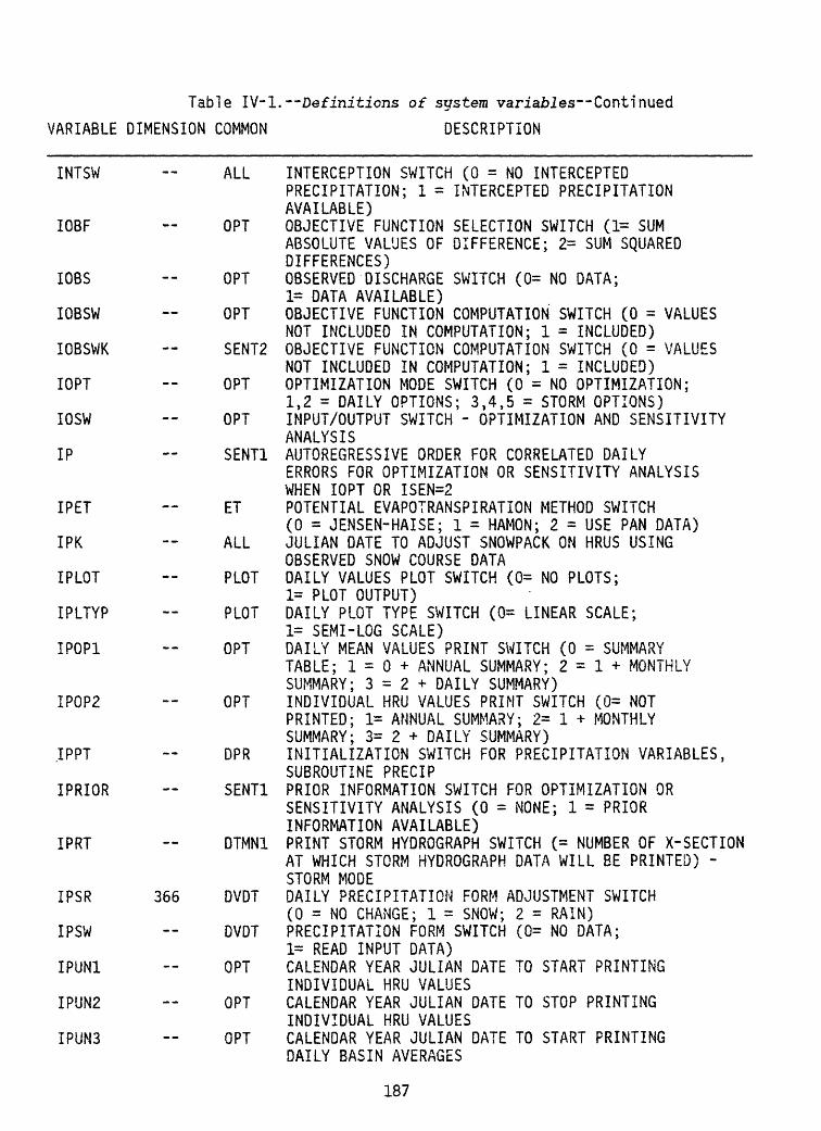
Table IV-1.--Definitions of system variables Continued
VARIABLE DIMENSION COMMON DESCRIPTION
INTSW
IOBF
IOBS
IOBSW
IOBSWK
IOPT
IOSW
IP
IPET
IPK
I PLOT
IPLTYP
IPOP1
IPOP2
IPPT
IPRIOR
IPRT
IPSR
IPSW
IPUN1
IPUN2
IPUN3
366
ALL INTERCEPTION SWITCH (0 = NO INTERCEPTEDPRECIPITATION; 1 = INTERCEPTED PRECIPITATIONAVAILABLE)
OPT OBJECTIVE FUNCTION SELECTION SWITCH (1= SUMABSOLUTE VALUES OF DIFFERENCE; 2= SUM SQUAREDDIFFERENCES)
OPT OBSERVED DISCHARGE SWITCH (0= NO DATA;1= DATA AVAILABLE)
OPT OBJECTIVE FUNCTION COMPUTATION SWITCH (0 = VALUESNOT INCLUDED IN COMPUTATION; 1 = INCLUDED)
SENT2 OBJECTIVE FUNCTION COMPUTATION SWITCH (0 = VALUESNOT INCLUDED IN COMPUTATION; 1 = INCLUDED)
OPT OPTIMIZATION MODE SWITCH (0 = NO OPTIMIZATION;1,2 = DAILY OPTIONS; 3,4,5 = STORM OPTIONS)
OPT INPUT/OUTPUT SWITCH - OPTIMIZATION AND SENSITIVITYANALYSIS
SENT1 AUTOREGRESSIVE ORDER FOR CORRELATED DAILYERRORS FOR OPTIMIZATION OR SENSITIVITY ANALYSISWHEN IOPT OR ISEN=2
ET POTENTIAL EVAPOTRANSPIRATION METHOD SWITCH(0 = JENSEN-HAISE; 1 = HAMON; 2 = USE PAN DATA)
ALL JULIAN DATE TO ADJUST SNOWPACK ON HRUS USINGOBSERVED SNOW COURSE DATA
PLOT DAILY VALUES PLOT SWITCH (0= NO PLOTS;1= PLOT OUTPUT)
PLOT DAILY PLOT TYPE SWITCH (0= LINEAR SCALE;1= SEMI-LOG SCALE)
OPT DAILY MEAN VALUES PRINT SWITCH (0 = SUMMARYTABLE; 1=0+ ANNUAL SUMMARY; 2=1+ MONTHLYSUMMARY; 3 = 2 + DAILY SUMMARY)
OPT INDIVIDUAL HRU VALUES PRINT SWITCH (0= NOTPRINTED; 1= ANNUAL SUMMARY; 2= 1 + MONTHLYSUMMARY; 3= 2 + DAILY SUMMARY)
DPR INITIALIZATION SWITCH FOR PRECIPITATION VARIABLES,SUBROUTINE PRECIP
SENT1 PRIOR INFORMATION SWITCH FOR OPTIMIZATION ORSENSITIVITY ANALYSIS (0 = NONE; 1 = PRIORINFORMATION AVAILABLE)
DTMN1 PRINT STORM HYDROGRAPH SWITCH (= NUMBER OF X-SECTIONAT WHICH STORM HYDROGRAPH DATA WILL BE PRINTED) -STORM MODE
DVDT DAILY PRECIPITATION FORM ADJUSTMENT SWITCH(0 = NO CHANGE; 1 = SNOW; 2 = RAIN)
DVDT PRECIPITATION FORM SWITCH (0= NO DATA;1= READ INPUT DATA)
OPT CALENDAR YEAR JULIAN DATE TO START PRINTINGINDIVIDUAL HRU VALUES
OPT CALENDAR YEAR JULIAN DATE TO STOP PRINTINGINDIVIDUAL HRU VALUES
OPT CALENDAR YEAR JULIAN DATE TO START PRINTINGDAILY BASIN AVERAGES
187

Table IV-1. Definitions of system variables Continued
VARIABLE DIMENSION COMMON DESCRIPTION
IPUN4 -- OPT CALENDAR YEAR JULIAN DATE TO STOP PRINTINGDAILY BASIN AVERAGES
IQ SENT1 MOVING AVERAGE FOR CORRELATED DAILY ERRORS FOROPTIMIZATION OR SENSITIVITY ANALYSIS WHEN IOPTOR ISEN=2
IR SENT1 IP + IQ FOR OPTIMIZATION OR SENSITIVITY ANALYSISWHEN IOPT OR ISE!*=2
IRD 50 RD SOLAR RADIATION PLANE ASSOCIATED WITH EACH HRU IRTYP 10 STOR TYPE OF ROUTING FOR EACH SURFACE RESERVOIR
(8 = PULS; 9 = LINEAR)IRU INDEX FOR SPECIFIC HYDROLOGIC RESPONSE UNIT IRUP1 10 STOR INDEX OF UPSTREAM SURFACE WATER STORAGE RESERVOIR 1
FOR EACH SURFACE WATER STORAGE RESERVOIR IRUP2 10 STOR INDEX OF UPSTREAM SURFACE WATER STORAGE RESERVOIR 2
FOR EACH SURFACE WATER STORAGE RESERVOIR IRUP3 10 STOR INDEX OF UPSTREAM SURFACE WATER STORAGE RESERVOIR 3
FOR EACH SURFACE WATER STORAGE RESERVOIR IS -- DFHSEG STORM EVENT INDEX - STORM MODE ISAVE VOL PRINT/PLOT RECORD COUNTER - STORM MODE ISBAS - SWITCH INITIALIZATION SWITCH, SUBROUTINE BASFLW ISEN OPT SENSITIVITY ANALYSIS SWITCH (0= NO ANALYSIS;
1, 2 = DAILY OPTIONS; 3,4= STORM OPTIONS) ISIM -- OPT SIMULATION MODE SWITCH (0= DAILY; 1,2,3=
STORM OPTIONS)ISNO SNO SNOW SWITCH (0 = NO SNOWPACK; 1 = SNOWPACK) ISNOSW -- OPSN02 INITIALIZATION SWITCH FOR SNOW VARIABLES, SUBROUTINE
SNOBALISNOYR -- OPSNO INITIALIZATION SWITCH, SUBROUTINE SNOBAL ISO 50 OPSN02 SNOWPACK MELT SWITCH FOR EACH HRU (1-
ACCUMULATION STAGE; 2= SPRING MELT STAGE) ISOIL 50 SM SOIL TYPE FOR EACH HRU (1=SAND; 2=LOAM;
3=CLAY) ISP1 -- SNO JULIAN DATE TO START LOOKING FOR SPRING SNOW
MELT STAGE. ISP2 SNO JULIAN DATE TO FORCE SNOWPACK TO SPRING SNOW
MELT STAGE.ISS SEQUENCE NUMBER OF STORM PERIOD - STORM MODE ISSOL -- OPT INITIALIZATION SWITCH, SUBROUTINE SOLRAD ISSRO SWITCH INITIALIZATION SWITCH, SUBROUTINE SRFRO ISSR1 - SWITCH SURFACE RUNOFF METHOD SWITCH (0 = LINEAR;
1 = NON-LINEAR) ISTAT SENT2 STATISTICAL SUMMARY SWITCH (0=NONE; 1=STATISTICAL
SUMMARY AT END OF RUN)ISTMP -- OPT INITIALIZATION SWITCH, SUBROUTINE TEMP ISUN SWITCH STORM SUBSURFACE AND GROUNDWATER ROUTING SWITCH
(0 = NOT DONE; 1 = SUBSURFACE AND GROUND WATERINCLUDED IN STORM COMPUTATION)
ISX1 SWITCH INITIALIZATION SWITCH, SUBROUTINE UNITD IT 50 ET TEST FOR START OF TRANSPIRATION PERIOD SWITCH
(0 = NO TEST; 1 = TEST SUM OF DAILY MAXTEMPERATURES VS TST)
188

Table IV-1. Definitions of system variables Continued
VARIABLE DIMENSION COMMON DESCRIPTION '
ITNDITRANS
ITST
ITSW
IUOUT
IWSWIWSW2IWYJDJDSJLDYJMJPLJPRJSOLJWDYJYKDKDSKFKFAKGW
KJDYKNTKRKRAKRES
KRSP
KSAT
KSTOR
KSVK.TKYRKl
K2
LBA
50
50
50
-- -- -- -- 50 5050
5050
50
50
50
ETSENT2
ET
ALL
OPT
OPTSENTSIZE
DATESALL
-_DTMN1DTMN1ALLALL
ALL
PCRCHABS
EXCBS
PCRCHABS
BS
STOR
--
EXC
PCRCHA
MONTH THAT TRANSPIRATION ENDS FOR EACH HRULOG TRANSFORMATION SWITCH FOR OPTIMIZATION ORSENSITIVITY ANALYSIS (0 = NO TRANSFORMATION OFRUNOFF VALUES; 1 = TRANSFORM)MONTH TO BEGIN CHECKING FOR START OF TRANSPIRATION FOR EACH HRUTRANSPIRATION SWITCH FOR EACH HRU (0 =VEGETATION DORMANT; 1= VEGETATION TRANSPIRING)STORE PREDICTED STORM VALUES SWITCH (0= NOSTORAGE; 1= STORE)INPUT/OUTPUT SWITCH-OPTIMIZATION AND SENSITIVITYWRITE SWITCH, OPTIMIZATION AND SENSITIVITY ANALYSISCURRENT WATER YEAR COUNTEREND DAY OF STORM PERIOD - STORM MODENUMBER OF RAIN GAGE DATA SETSJULIAN DATE, CALENDAR YEAR (1 = JANUARY 1)END MONTH OF STORM PERIOD - STORM MODEPLOT SWITCH (0 = NO PLOTS; 1 = PLOT) - STORM MODEPRINT SWITCH (0 = NO PRINT; 1 = PRINT) - STORM MODEJULIAN DATE, SOLAR YEAR (1 = DECEMBER 22)JULIAN DATE, WATER YEAR (1 = OCTOBER 1)END YEAR OF STORM PERIOD - STORM MODEBEGIN DAY OF HYDROGRAPH SEGMENT - STORM MODEINDEX OF RAIN GAGE ASSOCIATED WITH EACH HRUSEDIMENT PARAMETER FOR OVERLAND FLOW PLANEKF FOR EACH OVERLAND FLOW PLANEINDEX OF GROUND WATER RESERVOIR RECEIVING SEEPAGEFROM EACH HRUJULIAN DAY TO READ IN CHANGES TO HRU PARAMETERSNUMBER OF HRUS WITH SNOW COVERSEDIMENT PARAMETER FOR OVERLAND FLOW PLANEKR FOR EACH OVERLAND FLOW PLANEINDEX OF SUBSURFACE RESERVOIR RECEIVING SEEPAGEFROM EACH HRUINDEX OF GROUND WATER RESERVOIR RECEIVING SEEPAGEFROM EACH SUBSURFACE RESERVOIRHYDRAULIC CONDUCTIVITY OF TRANSMISSION ZONE(INCHES/HOUR) - STORM MODEINDEX OF SURFACE WATER RESERVOIR RECEIVING RUNOFFFROM EACH HRUJULIAN DAY FOR. PRECIPITATION FORM ADJUSTMENTBEGIN TIME OF HYDROGRAPH SEGMENT - STORM MODECALENDAR YEAR TO READ IN CHANGES TO HRU PARAMETERSNUMBER OF DAYS IN WATER YEAR FOR PRECIPITATIONFORM ADJUSTMENT TO SNOWNUMBER OF DAYS IN WATER YEAR FOR PRECIPITATION FORMADJUSTMENT TO RAININDEX OF OVERLAND FLOW SEGMENT TO 3E USED AS INPUTTO CHANNEL SEGMENT - STORM MODE
189

Table IV-l.--Definitions of system variables Continued
VARIABLE DIMENSION COMMON DESCRIPTION
LBC -- I.D. OF OVERLAND FLOW PLANE PROVIDING LATERAL INFLOW
TO CHANNEL SEGMENT - STORM MODELD END DAY OF HYDROGRAPH SEGMENT - STORM MODE LMO SIZE PREVIOUS MONTH COUNTERLOP 20 OPT INDEX NUMBER OF PARAMETER TO BE OPTIMIZED LSO 50 OPSN02 COUNTER FOR CONSECUTIVE DAYS OF ISOTHERMAL
SNOWPACK FOR EACH HRU (5= START SPRING MELT STAGE) LST 50 OPSNO SNOWPACK ALBEDO ADJUSTMENT SWITCH (0 = NO ADJUSTMENT
1 = ADJUST FOR SHALLOW SNOWFALL)LT -- END TIME OF HYDROGRAPH SEGMENT - STORM MODE LYR SIZE PREVIOUS YEAR COUNTER MB DATES BEGIN MONTH OF WATER YEAR MDY -- ALL DAY OF MONTH ME DATES END MONTH OF WATER YEARMFN OPT END MONTH OF OBJECTIVE FUNCTION COMPUTATION MFS OPT BEGIN MONTH OF OBJECTIVE FUNCTION COMPUTATION MMA 50 PCRCHA SEDIMENT PARAMETER FOR OVERLAND FLOW PLANE - STORM
MODEMO -- ALL CURRENT MONTH COUNTERMPCN DPR MONTH THAT OVERRIDE OF DRCOR AND DSCOR ENDS MPCS -- DPR MONTH THAT OVERRIDE OF DRCOR AND DSCOR BEGINS MPC1 DPR OVERRIDE SWITCH FOR DRCOR AND DSCOR (0= NON-
OVERRIDE PERIOD; 1= OVERRIDE PERIOD) MRDC RD SWITCH TO DETERMINE METHOD USED TO COMPUTE SOLAR
RADIATION FOR MISSING DAYS (0= RADIATION DATA NOTUSED; 1= DEGREE - DAY; 2= SKY COVER)
MSO 50 OPSN02 ENERGY BALANCE SWITCH FOR EACH HRU (l^WINTER PERIOD;2 = BEGIN LOOKING FOR SPRING MELT PERIOD)
MTSE -- ET MONTH THAT THUNDERSTORM TYPE EVENTS END MTSS ET MONTH THAT THUNDERSTORM TYPE EVENTS START MXDY -- ALL NUMBER OF DAYS IN YEAR MYR ALL CURRENT CALENDER YEARNCRSEG VOL NUMBER OF CHANNEL ROUTING SEGMENTS - STORM MODE ND BEGIN DAY OF STORM PERIOD - STORM MODE NDELSA 100 PCRCHA NUMBER OF TIME INCREMENTS FOR ROUTING FOR EACH
OVERLAND FLOW AND CHANNEL SEGMENT - STORM MODENDOP OPT OPTIMIZATION SWITCH (0= CONTINUE; 1= END) NDS ALL NUMBER OF RAIN GAGE DATA SET NDSN SENT SENSITIVITY ANALYSIS SWITCH (0= CONTINUE;
1= END)NDTY SIZE NUMBER OF DATA TYPES USED IN SIMULATION NDVR 20,50 SENT1 INDICES OF DISTRIBUTED PARAMETERS TO BE ADJUSTED IN
OPTIMIZATION AND SENSITIVITY ANALYSIS NDX NUMBER OF INTERVALS TO SUBDIVIDE OVERLAND FLOW
PLANES OR CHANNEL SEGMENT FOR FINITE-DIFFERENCECALCULATIONS - STORM MODE
NDY 12 SIZE NUMBER OF DAYS IN EACH MONTH NGW -- BS NUMBER OF GROUND WATER STORAGE RESERVOIRS NIRU IRU ASSOCIATED WITH OVERLAND FLOW PLANE - STORM
MODE
190

Table IV-1. Definitions of system variables Continued
VARIABLE DIMENSION COMMON DESCRIPTION
MMNMOBF
NOBF
NOFSEGNPRNT
NRDNREC
NRESNRUNS
NSOS
NSPNST
NSTORNSWNTRYNVNVAR
NXSA
NYNYRNYRI
OBFOBFOPTOBPKOBROOBSRUN
ODELSA
OFIPA
OFLTORAD
ORO02
__
-_
_
10
50 20
100
--
10 5050
366
100
50
50
10,10
BEGIN MONTH OF STORM PERIOD - STORM MODESENT NUMBER OF MONTHS IN DAILY OBJECTIVE FUNCTION FOR
OPTIMIZATIONSENT NUMBER OF DAYS OR EVENTS INCLUDED IN OBJECTIVE
FUNCTION FOR OPTIMIZATIONVOL NUMBER OF OVERLAND FLOW PLANES - STORM MODEOPT PRINT SWITCH DURING OPTIMIZATION (0= NO PRINT;
1= PRINT)RD NUMBER OF SOLAR RADIATION PLANESSENT2 INDEX FOR DIRECT ACCESS FILE USED IN OPTIMIZATION
OR SENSITIVITY ANALYSISBS NUMBER OF SUBSURFACE STORAGE RESERVOIRSALL NUMBER OF HYDROLOGIC RESPONSE UNITSDFHSEG NUMBER OF HYDROGRAPH SEGMENTS IN A STORM PERIOD -
STORM MODESTOR NUMBER OF STORAGE- OUT FLOW VALUES IN TABLE FOR PULS
ROUTING OF SURFACE-WATER RESERVOIR NUMBER OF STORM PERIODS - STORM MODE
VOL TOTAL NUMBER OF HYDROGRAPH SEGMENTS IN ALL STORMEVENTS - STORM MODE
STOR NUMBER OF SURFACE WATER STORAGE RESERVOIRSSNOPSENT1 NUMBER OF ADJUSTMENTS PER PARAMETER FOR OPTIMIZATIONSENT NUMBER OF PARAMETERS TO BE OPTIMIZEDSENT1 NUMBER OF VALUES OF A DISTRIBUTED PARAMETER TO BE
ADJUSTED DURING OPTIMIZATIONPCRCHA NUMBER OF CROSS-SECTIONS FOR ROUTING FOR EACH
OVERLAND FLOW AND CHANNEL SEGMENT - STORM MODE BEGIN YEAR OF STORM PERIOD - STORM MODE
SIZE NUMBER OF WATER YEARS TO BE SIMULATEDOPT NUMBER OF YEARS IN INITIALIZATION PERIOD
OPTIMIZATION OR SENSITIVITY ANALYSISOPT COMPUTED OBJECTIVE FUNCTIONSSENT2 FINAL OBJECTIVE FUNCTION VALUE FOR OPTIMIZATIONVOL OBSERVED STORM PEAK (CFS) - STORM MODEVOL OBSERVED STORM RUNOFF VOLUME (INCHES) - STORM MODESENT1 OBSERVED RUNOFF ARRAY USED IN OPTIMIZATION AND
SENSITIVITY ANALYSISPCRCHA NUMBER OF TIME INCREMENTS FOR PRINT OR PLOT FOR EACH
OVERLAND FLOW AND CHANNEL SEGMENT - STORM MODEPCRCHA PORTION OF OVERLAND FLOW PLANE THAT IS IMPERVIOUS
(DECIMAL PERCENT) - STORM MODESED TOTAL AREA FOR EACH OVERLAND FLOW PLANE - STORM MODEALL COMPUTED SHORTWAVE RADIATION ON HORIZONTAL SURFACE
(LANGLEYS)ALL DAILY VALUE OF OBSERVED DISCHARGE (CFS)STOR OUTFLOW- STORAGE TABLE VALUES FOR PULS ROUTING
191

Table IV-1. Definitions of system variables Continued
VARIABLE DIMENSION COMMON DESCRIPTION
P 20 SENT1 INITIAL ADJUSTMENT FACTOR FOR EACH PARAMETERFOR OPTIMIZATION
PACT 50 SNO SNOWPACK TEMPERATURE (DEGREES C), EACH HRU PARMCA 10 SIZE FIVE DIGIT CODE TO IDENTIFY EACH TYPE OF INPUT
CLIMATE, PRECIPITATION AND DISCHARGE DATA PARM1 KINEMATIC PARAMETER ALPHA FOR TYPE = 4 OR WIDTH
OF CHANNEL FOR CHANNEL TYPE = 1 OR 3 - STORM MODEPARM2 KINEMATIC PARAMETER M FOR TYPE = 4 - STORM MODE PARS RD CORRECTION FACTOR FOR COMPUTED SOLAR RADIATION
ON SUMMER DAY WITH PRECIPITATION (DECIMALPERCENT)
PARW RD CORRECTION FACTOR FOR COMPUTED SOLAR RADIATIONON WINTER DAY WITH PRECIPITATION (DECIMALPERCENT)
PAT 12 DPR MAXIMUM AIR TEMPERATURE, WHICH WHEN EXCEEDED,FORCES PRECIPITATION TO BE ALL RAIN
PCONR DPR OVERRIDE VALUE FOR RAINFALL ADJUSTMENT FACTOR DRCORWHEN MPC1=1
PCONS DPR OVERRIDE VALUE FOR SNOWFALL ADJUSTMENT FACTOR DSCORWHEN MPC1=1
PCOR CORRECTION FACTOR FOR PRECIPITATION ON AN HRU PCRID IDENTIFICATION CHARACTERS FOR OVERLAND FLOW
PLANES, CHANNEL AND RESERVOIR SEGMENTS ANDJUNCTIONS - STORM MODE
PCRIDA 100 PCRCHA PCRID FOR EACH PLANE, CHANNEL, RESERVOIR ORJUNCTION - STORM MODE
PERV 50 UPR PERCENT OF PERVIOUS AREA ON EACH HRU (DECIMAL) PET 50 ALL COMPUTED POTENTIAL EVAPOTRANSPIRATION FOR EACH
HRU (INCHES) PHI 10 SENT2 ARRAY OF AUTOREGRESSIVE AND MOVING AVERAGE
PARAMETERS FOR OPTIMIZATION AND SENSITIVITY ANALYSIS PICE 50 SNO PORTION OF SNOWPACK EXISTING AS ICE ON EACH HRU
(INCHES) PINC SENT1 FRACTION BY WHICH PARAMETERS ARE ADJUSTED IN A
SENSITIVITY ANALYSIS PKAD 50 SNOP ADJUSTED SNOWPACK WATER EQUIVALENT COMPUTED FROM
OBSERVED SNOW COURSE DATA PKDEF 50 SNO CALORIES REQUIRED TO BRING PACK TO ISOTHERMAL
STATE, EACH HRUPLMN PLOT MINIMUM VALUE FOR DAILY PLOT PLMX PLOT MAXIMUM VALUE FOR DAILY PLOT PP ALL AREA WEIGHTED PRECIPITATION FOR BASIN (INCHES) PPAR 5 DPR AREA ASSOCIATED WITH EACH PRECIPITATION GAGE (ACRES) PPT ~ ALL MEASURED PRECIPITATION (INCHES) PPTI 50 ALL ADJUSTED PRECIPITATION FOR IMPERVIOUS AREA OF EACH
HRU (INCHES) PQ 50 SED TOTAL ROUTED FLOW FOR EACH STORM PERIOD (INCHES) -
STORM MODE PRMX 50 SNOP PERCENT OF TOTAL PRECIPITATION IN A MIXED RAIN-SNOW
EVENT THAT IS RAIN (DECIMAL)
192

Table IV-1. Definitions of system variables Continued
VARIABLE DIMENSION COMMON DESCRIPTION
PRORO
PROUTA PRPRO
PRTIN
PRTINA PRTOUT
PSED
PSN
PSP
PSS
PTF
PTN PWEQV
QA
QCOND
QLAT
QMXA
QQI
QRO
QSDY QSID
QSIO
QSMO
366 PLOT OBSERVED MEAN DISCHARGE VALUES FOR EACH DAY OF WATERYEAR (CFS)
100 PCRCHA PRTOUT FOR EACH ROUTING SEGMENT - STORM MODE 366 PLOT PREDICTED MEAN DISCHARGE VALUES FOR EACH DAY OF
WATER YEAR (CFS) SWITCH TO PRINT OR PLOT INFLOW TO ROUTING
SEGMENTS - STORM MODE (0 = NONE; 1 = PRINT; 2 = PLOT)
100 PCRCHA PRTIN FOR EACH ROUTING SEGMENT - STORM MODE SWITCH TO PRINT OR PLOT OUTFLOW TO ROUTING
SEGMENTS - STORM MODE (0 = NONE; 1 = PRINT;2 = PLOT)
50 SED TOTAL ROUTED SEDIMENT LOAD FOR EACH STORM PERIOD(TONS) - STORM MODE
50 SNOP WATER EQUIVALENT OF NEW SNOW ON EACH HRU(INCHES)
COMBINED EFFECT OF MOISTURE DEFICIT ANDCAPILLARY POTENTIAL (INCHES) - STORM MODE
50 OPSNO ACCUMULATED SUM OF NET PRECIPITATION BEGINNING ON THE FIRST DAY OF SNOWPACK FORMATION
PRECIPITATION WHICH FALLS THROUGH VEGETATION CANOPY(INCHES)
50 ALL NET PRECIPITATION FOR EACH HRU (INCHES) 50 SNO WATER EQUIVALENT OF SNOWPACK ON EACH HRU
(INCHES) 1440 UNITRF ROUTED OUTFLOW FOR AN OVERLAND FLOW OR CHANNEL
SEGMENT FOR 1-60 MINUTE INTERVALS (CFS/FT) - STORM MODEHEAT CONDUCTION BETWEEN SNOW SURFACE AND SNOWPACK (CALORIES)ACCUMULATED LATERAL INFLOW TO A CHANNEL SEGMENT FOR FLOW ROUTING FOR 1-60 MINUTE INTERVALS (CFS/FT) STORM MODEMAXIMUM ROUTED DISCHARGE FOR EACH OVERLAND FLOW OR CHANNEL SEGMENT FOR A STORM EVENT - STORM MODE INITIAL DISCHARGE VALUES FOR EACH X-SECTION OF EACH OVERLAND FLOW AND CHANNEL SEGMENT - STORM MODE INITIAL FLOW VALUE FOR EACH X-SECTION FOR IMPERVIOUS AREA OF EACH OVERLAND FLOW PLANE - STORM MODE INITIAL DAY MEAN OUTFLOW FOR EACH SURFACE STORAGE RESERVOIR (CFS)
QSOUT DAY OF OUTPUT RECORD FOR PLOT OR PRINT - STORM MODEQSOUT OVERLAND FLOW OR CHANNEL SEGMENT ID FOR OUTPUT
RECORD FOR PLOT OR PRINT - STORM MODEQSOUT INFLOW/OUTFLOW SWITCH FOR OUTPUT RECORD FOR PLOT OR
PRINT (1 = INFLOW TO SEGMENT; 2 = OUTFLOW) - STORM MODE
QSOUT MONTH OF OUTPUT RECORD FOR PLOT OR PRINT - STORM MODE
1440 UNITRF
100
11,100
11,50
10
INITCD
INITCD
INITCD
STOR
193

Table IV-1. Definitions of system variables Continued
VARIABLE DIMENSION COMMON DESCRIPTION
QSQS QSOUT TYPE SWITCH FOR OUTPUT RECORD FOR PLOT OR PRINT(1 = PRINT DISCHARGE; 2 = PRINT SEDIMENT; 3 = PLOTDISCHARGE; 4 = PLOT SEDIMENT) - STORM MODE
QSRPD QSOUT VALUES PER DAY FOR OUTPUT RECORD FOR PLOT OR PRINT- STORM MODE
QSWY QSOUT WATER YEAR OF OUTPUT RECORD FOR PLOT OR PRINT -STORM MODE
RAD 20,13 RD POTENTIAL SHORTWAVE RADIATION FOR EACH SOLARRADIATION PLANE FOR 13 DATES (LANGLEYS)
RAJ -- RATIO OF ACTUAL TO POTENTIAL SOLAR RADIATION FORA HORIZONTAL SURFACE
RAS 3S DAILY SUBSURFACE FLOW FOR ALL SUBSURFACE RESERVOIRS(ACRE-INCHES)
RASQ 50 BS DAILY SUBSURFACE FLOW FROM EACH SUBSURFACERESERVOIR (ACRE-INCHES)
RBA 50 PCRCHA INDEX OF OVERLAND FLOW SEGMENT TO BE USED ASINPUT TO CHANNEL SEGMENT - STORM MODE
RBC I.D. OF OVERLAND FLOW PLANE PROVIDING LATERAL INFLOWTO CHANNEL SEGMENT - STORM MODE
RGB 50 BS ROUTING COEFFICIENT FOR EACH GROUNDWATERRESERVOIR
RCF 50 BS LINEAR ROUTING COEFFICIENT FOR EACH SUBSURFACERESERVOIR
RCP 50 BS , NON-LINEAR ROUTING COEFFICIENT FOR EACH SUB SURFACE RESERVOIR
RCS 10 STOR SURFACE STORAGE RESERVOIR LINEAR ROUTING COEFFICIENTFOR EACH RESERVOIR
RC1 - AVERAGE BASEFLOW OR PEAK DISCHARGE WHEN IC2 = 0OR 1 - STORM MODE
RC2 VOLUME OF RUNOFF IN INCHES PER SQUARE MILE WHENIC2 = 1 - STORM MODE
RDB RD COEFFICIENT USED IN SKY COVER - SOLAR RADIATIONRELATION
RDC 12 RD Y - INTERCEPT FOR RELATION BETWEEN TEMPERATURE(X) AND 1) DEGREE DAY (Y) OR 2) SKY COVER (Y)WHEN MRDC = 1 OR 2
RDM 12 RD SLOPE FOR RELATION BETWEEN TEMPERATURE (X) AND1) DEGREE DAY (Y) OR 2) SKY COVER (Y) WHENMRDC = 1 OR 2
RDMX RD MAXIMUM PERCENT OF POTENTIAL SOLAR RADIATION(DECIMAL)
RDP RD COEFFICIENT USED IN SKY COVER - SOLAR RADIATIONRELATION
RECHR 50 SM STORAGE IN UPPER PART OF SOIL PROFILE WHERELOSSES OCCUR AS EVAPORATION AND TRANSPIRATION(INCHES)
REMX 50 SM MAXIMUM VALUE OF RECHR FOR EACH HRU (INCHES) RES 50 BS STORAGE IN EACH SUBSURFACE RESERVOIR
(ACRE-INCHES)
194

Table IV-1. Definitions of system variables Continued
VARIABLE DIMENSION COMMON DESCRIPTION
RESMX
RETIP
REXP
RFL
RGF
RITEA
RMXA
RMXM
RNSTS
RNSTW
RQDRSEP
RSTOR
SASALBSASSCN
SCT
sexSCI
SEP
SETCCNSFL
SGW
50
50
50
-_
--
50
50
50
--50
50
5050--50
50
50
50
50
--
--
BS
IMPRV
BS
DFHSEG
PCRCHA
SNOP
SNOP
DPR
DPR
SED
IMPRV
WXOPSNOSMSM
SM
SM
SM
BS
SNODFHSEG
BS
COEFFICIENT FOR ROUTING WATER FROM EACH SUBSURFACE RESERVOIR TO GROUNDWATER RESERVOIRMAXIMUM RETENTION STORAGE ON IMPERVIOUS AREA FOREACH HRU (INCHES)COEFFICIENT FOR ROUTING WATER FROM EACH SUBSURFACE RESERVOIR TO GROUNDWATER RESERVOIRREAD FLAG FOR CONTINUATION OF STORM HYDROGRAPHFROM PREVIOUS DAY - STORM MODERATIO OF COMBINED EFFECTS OF MOISTURE DEFICIT ANDCAPILLARY POTENTIAL AT WETTING FRONT FROM WILTINGPOINT TO FIELD CAPACITY - STORM MODEWRITE SWITCH FOR EACH CHANNEL, RESERVOIR ORJUNCTION (0 = NO STORAGE; 1 = OUTPUT DATA STOREDFOR INPUT TO SUBSEQUENT SEGMENT) - STORM MODEPROPORTION OF RAIN IN RAIN/SNOW EVENT ABOVE WHICHSNOW ALBEDO IS NOT RESET FOR SNOWPACK ACCUMULATIONSTAGEPROPORTION OF RAIN IN RAIN/SNOW EVENT ABOVEWHICH SNOW ALBEDO IS NOT RESET FOR SNOWPACK MELTSTAGEINTERCEPTION STORAGE CAPACITY OF UNIT AREA OFVEGETATION FOR RAIN DURING SUMMER PERIOD, FOR EACHHRU (INCHES)INTERCEPTION STORAGE CAPACITY OF UNIT AREA OFVEGETATION FOR RAIN DURING WINTER PERIOD FOR EACHHRU (INCHES)DAILY ROUTED FLOW DURING STORM PERIOD - STORM MODESEEPAGE RATE FROM EACH SUBSURFACE RESERVOIR TOGROUND WATER RESERVOIR (INCHES/DAY)RETENTION STORAGE ON IMPERVIOUS AREA FOR EACHHRU (INCHES)SLOPE AND ASPECT FOR EACH RADIATION PLANEALBEDO ON DAY PRIOR TO LAST SNOW FOR EACH HRUTOTAL SURFACE RUNOFF FROM ALL HRUS (ACRE-INCHES)MINIMUM CONTRIBUTING AREA FOR SURFACE RUNOFF WHENISSR1 = 0; COEFFICIENT IN CONTRIBUTING AREA - SOILMOISTURE INDEX RELATION WHEN ISSR1 = 1DIFFERENCE BETWEEN MAXIMUM AND MINIMUM CONTRIBUTINGAREA FOR SURFACE RUNOFF FOR EACH HRUMAXIMUM POSSIBLE CONTRIBUTING AREA FOR SURFACERUNOFF AS PROPORTION OF EACH HRUCOEFFICIENT IN SURFACE RUNOFF CONTRIBUTING AREA -SOIL MOISTURE INDEX RELATIONSEEPAGE RATE FROM SOIL MOISTURE EXCESS TO EACHGROUNDWATER RESERVOIR (INCHES/DAY)SNOWPACK SETTLEMENT TIME CONSTANTSTORE FLAG FOR CONTINUATION OF HYDROGRAPH TO NEXTDAY - STORM MODETOTAL DAILY GROUNDWATER FLOW FROM ALL GROUNDWATERRESERVOIRS (ACRE-INCHES)
195

Table IV-1. Definitions of system variables Continued
VARIABLE DIMENSION COMMON DESCRIPTION
SIMOPT SLP SLST SMAV
SMAX
SMLT SMSA
SMVOPT
SNEV SNST
SNSV SCLF
SRO SRS
SRX
SSGW
SSH
STAIDC
STAIDP
STATCA
STOSWRDSX
S15
S2
S24
55
3 VOL NOT CURRENTLY USED 50 SM SLOPE OF EACH HRU (DECIMAL PERCENT) 50 OPSNO NUMBER OF DAYS SINCE LAST SNOWFALL ON EACH HRU 50 SM DAILY AVAILABLE WATER IN SOIL PROFILE FOR EACH HRU
(INCHES) 50 SM MAXIMUM AVAILABLE WATER HOLDING CAPACITY OF SOIL
PROFILE FOR EACH HRU (INCHES)50 SNO DAILY SNOWMELT FOR EACH HRU (INCHES) 50 DSM ACCUMULATED INFILTRATION FOR EACH HRU (INCHES)
- STORM MODE 366 SENT1 PREDICTED RUNOFF PRODUCED FROM FINAL PARAMETER
VALUES OBTAINED IN OPTIMIZATION50 SNO EVAPORATION FROM SNOWPACK FOR EACH HRU (INCHES) 50 DPR INTERCEPTION STORAGE CAPACITY OF UNIT AREA OF
VEGETATION FOR SNOW, FOR EACH HRU (INCHES, WATER EQUIVALENT)
50 OPSNO DEPTH OF NEW SNOW ON EACH HRU (INCHES) RATIO OF ACTUAL TO POTENTIAL SOLAR RADIATION FOR
A HORIZONTAL SURFACE 50 SM SURFACE RUNOFF FROM EACH HRU (INCHES)
BS TOTAL DAILY SUBSURFACE FLOW FROM ALL SUBSURFACERESERVOIRS (ACRE-INCHES)
50 SM MAXIMUM DAILY SNOWMELT INFILTRATION CAPACITY OF SOILPROFILE AT FIELD CAPACITY FOR EACH HRU (INCHES)
BS TOTAL FLOW FROM ALL SUBSURFACE RESERVOIRS TOGROUND-WATER RESERVOIRS FOR WATER YEAR (INCHES)
20,13 ET HOURS BETWEEN SUNRISE AND SUNSET FOR EACH RADIATIONPLANE FOR 13 DATES
32 SIZE ARRAY OF 16 DIGIT STATION IDENTIFICATION NUMBERS FORCLIMATE DATA
8,5 SIZE ARRAY OF 16-DIGIT STATION IDENTIFICATION NUMBERSFOR PRECIPITATION DATA
10 SIZE FIVE DIGIT CODE USED IN CONJUNCTION WITH PARMCA TODISTINGUISH INPUT DATA TYPES
10 STOR INITIAL STORAGE IN EACH SURFACE RESERVOIR (CFS-DAYS) 50 ALL COMPUTED SW RADIATION FOR EACH HRU (LANGLEYS) 50 BS PORTION OF SNOWMELT THAT BECOMES SURFACE RUNOFF
(INCHES)SLOPE OF LINE DRAWN BETWEEN TWO ADJACENT POINTS IN THE PULS ROUTING TABLE FOR 15 MINUTE RESERVOIR ROUTING - STORM MODE
10,10 STOR STORAGE VALUES IN OUTFLOW/STORAGE TABLE FOR PULSROUTING (CFS DAYS)
10,10 STOR SLOPE OF LINE DRAWN BETWEEN TWO ADJACENT POINTS INTHE PULS ROUTING TABLE FOR 24 HOUR RESERVOIR ROUTING
10,10 STOR SLOPE OF LINE DRAWN BETWEEN TWO ADJACENT POINTS IN THE PULS ROUTING TABLE FOR 5 MINUTE RESERVOIR ROUTING - STORM MODE
10,10 STOR
196

Table IV-1. Definitions of system variables Continued
VARIABLE DIMENSION COMMON DESCRIPTION
TA
TAVCTAVFTCAL
TCRN
TCRX
TESTNO
THRES
THRESA
TITLTLAT
TIN
TIPSTLX
TMN
TMNFTMX
TMXFTNAJ
TRNCF
TSM
TST
TSUW
TT
TXAJ
TYPE
1440
505050
....
50
100
181440
12
-_12
--
50--
5050
50
50
50
50
11,100
50
_-
UNITRF ROUTED SEDIMENT OUTFLOW FOR AN OVERLAND FLOW ORCHANNEL SEGMENT FOR 1-60 MINUTE INTERVALS(KG/CU.FT./S) - STORM MODE
ALL DAILY AVERAGE TEMPERATURE FOR EACH HRU (DEGREES C)ALL DAILY AVERAGE TEMPERATURE FOR EACH HRU (DEGREES F)SNO DAILY NET ENERGY BALANCE FOR EACH HRU WITH
SNOW MONTHLY MINIMUM TEMPERATURE ADJUSTMENT FACTOR FOR
AN HRU (DEGREES C OR F) MONTHLY MAXIMUM TEMPERATURE ADJUSTMENT FACTOR FOR
AN HRU (DEGREES C OR F)OPT SWITCH TO INCLUDE STORM IN OPTIMIZATION OR
SENSITIVITY ANALYSIS (0= NOT INCLUDED; 1= INCLUDED) MINIMUM DEPTH OF FLOW FOR CONTINUATION OF ROUTING
(FT) - STORM MODEPCRCHA THRES FOR EACH OVERLAND FLOW PLANE OR CHANNEL
ROUTING SEGMENT (FT) - STORM MODESIZE TITLE FOR PRINTED OUTPUT (UP TO 70 CHARACTERS)UNITRF LATERAL SEDIMENT INFLOW TO A CHANNEL SEGMENT FOR
SEDIMENT ROUTING FOR 1-60 MINUTE INTERVALS(KG/SQ.FT./S) - STORM MODE
WX LAPSE RATE FOR MINIMUM DAILY TEMPERATURE FOR MONTHS1-12 (DEGREES C OR F)
WX NOT CURRENTLY USEDWX LAPSE RATE FOR MAXIMUM DAILY AIR TEMPERATURE FOR
MONTHS 1-12 (DEGREES C OR F)WX DAILY MINIMUM TEMPERATURE MEASURED AT CLIMATE
STATION (DEGREES C OR F)ALL DAILY MINIMUM TEMPERATURE FOR EACH HRU (DEGREES F)WX DAILY MAXIMUM TEMPERATURE MEASURED AT CLIMATE
STATION (DEGREES C OR F)ALL DAILY MAXIMUM TEMPERATURE FOR EACH HRU (DEGREES F)WX ADJUSTMENT FOR MINIMUM AIR TEMPERATURE FOR SLOPE AND
ASPECT FOR EACH HRU (DEGREES C OR F)SNO TRANSMISSION COEFFICIENT FOR SHORTWAVE RADIATION
THROUGH VEGETATION CANOPY FOR EACH HRUSENT2 SUM OF DAILY MAXIMUM TEMPERATURE TO DETERMINE START
OF ACTIVE ET PERIOD FOR EACH HRUET ACCUMULATED DAILY MAXIMUM TEMPERATURE VALUE FOR
MONTH ITST AT WHICH TRANSPIRATION BEGINS FOR EACHHRU
SED SEDIMENT LOAD FROM EACH OVERLAND FLOW PLANE(TONS/DAY) - STORM MODE
INITCD INITIAL SEDIMENT VALUES FOR EACH X-SECTION FOR EACHOVERLAND FLOW AND CHANNEL SEGMENT (KG/CU.FT)- STORM MODE
WX ADJUSTMENT FOR MAXIMUM AIR TEMPERATURE FOR SLOPE ANDASPECT FOR EACH HRU (DEGREES C OR F)
TYPE OF OVERLAND FLOW PLANE OR CHANNEL ROUTINGSEGMENT - STORM MODE
197

Table IV-1. Definitions of system variables Continued
VARIABLE DIMENSION COMMON DESCRIPTION
TYPEA
UGS
UINF
UNBAS
UPA
UPCORUPE
UPSWA
UP1
UP2
UPS
USS
UVWY
VBIN
WCTXWVD
WV15
WV5
WYWYDXXINXINLOSXOPT
XX
XXAVE
XXDEV
ZINFCZINV
100
50
50,96
50,96
50,3
501440
50
--
50
367
20,20
10,10
10,10
10,10
5,50505020
20
20
20,50
20,2020,20
PCRCHA TYPE FOR EACH OVERLAND FLOW PLANE OR CHANNEL ROUTINGSEGMENT - STORM MODE
BS SEEPAGE TO GROUND WATER RESERVOIRS FROM EACH HRU(INCHES)
UNSS SUBSURFACE FLOW FOR EACH SUBSURFACE RESERVOIR AT15 MINUTE INTERVALS (INCHES) - STORM MODE
UNSS GROUND WATER FLOW FOR EACH GROUND WATER RESERVOIRAT 15 MINUTE INTERVALS (INCHES) - STORM MODE
PCRCHA UPSTREAM INFLOW SEGMENT I.D.S FOR EACH CHANNELROUTING SEGMENT - STORM MODE
UPR STORM PRECIPITATION CORRECTION FACTOR FOR EACH HRUUNITRF PRECIPITATION EXCESS FOR 1 TO 15 MINUTE INTERVALS
(INCHES) - STORM MODEPCRCHA UPSTREAM INFLOW SWITCH FOR EACH CHANNEL ROUTING
SEGMENT - STORM MODE (0 = NONE; 1 = UPSTREAM INFLOW) UPSTREAM INFLOW SEGMENT FOR CHANNEL ROUTING SEGMENT
- STORM MODE UPSTREAM INFLOW SEGMENT FOR CHANNEL ROUTING SEGMENT
- STORM MODE UPSTREAM INFLOW SEGMENT FOR CHANNEL ROUTING SEGMENT
- STORM MODEBS SEEPAGE TO SUBSURFACE RESERVOIRS FROM EACH HRU
(INCHES)UVRT STORM VALUES SWITCH FOR EACH DAY OF WATER YEAR - STO
MODE (0 = NONE; 1 = PRECIPITATION; 2 = PRECIPITATIONAND DISCHARGE)
SENT1 PRIOR INFORMATION COVARIANCE MATRIX FOR OPTIMIZATIONOR SENSITIVITY ANALYSIS
ET NOT CURRENTLY USEDSTOR CALCULATED TABLE VALUES OF (2S/DT + 0) TO DETERMINE
OUTFLOW FOR DAILY PULS ROUTINGSTOR CALCULATED TABLE VALUES OF (2S/DT + 0) TO DETERMINE
OUTFLOW FOR 15 MINUTE PULS ROUTINGSTOR CALCULATED TABLE VALUES OF (2S/DT + 0) TO DETERMINE
OUTFLOW FOR 5 MINUTE PULS ROUTINGDFHSEG WATER YEAR OF STORM EVENT - STORM MODE WATER YEAR DAY OF STORM EVENT - STORM MODE
VOL INFILTRATION PARAMETERS FOR EACH HRU - STORM MODEDPR INTERCEPTION FOR EACH HRU (INCHES)ALL INTERCEPTION LOSS FOR EACH HRU (INCHES)SENT FINAL VALUES OF PARAMETERS OBTAINED FROM
OPTIMIZATIONSENT ARRAY OF PARAMETERS FOR OPTIMIZATION OR SENSITIVITY
ANALYSISSENT1 AVERAGE VALUE OF DISTRIBUTED PARAMETERS FOR
OPTIMIZATION OR SENSITIVITY ANALYSISSENT1 DEVIATION OF DISTRIBUTED PARAMETERS FROM AVERAGE FOR
OPTIMIZATION OR SENSITIVITY ANALYSISSENT1 INFORMATION MATRIX FOR SENSITIVITY ANALYSISSENT1 INVERSE OF INFORMATION MATRIX FOR SENSITIVITY
ANALYSIS
198

ATTACHMENT VI
System labeled COMMON areas
The labeled common areas used in PRMS, the variables included in each common area and the subroutines in which they are used are listed in table VI-1.
Table VI-1. System labeled common areas
COMMON
ALL
BS
DATES
DATOP
VARIABLES
SCODEDIRLITSW(50)KDS(50)MYROROPTN(50)TMNF(50)
ARG(50)GWSKRSP(50)RCB(50)SEP(50)UGS(50)KRSBASQ(50)
BYREMOIDB
BYRINEMOINBDYOPIGOPT
PPTI(SO)HORADJLDYMDYNDSPET(50)SWRD(50)TMXF(50)
ARS(50)KGW(50)NGWRCF(50)SGWUSS(50)EXSS(50)RASQ(50)
BMOEDYIDE
BMOINEDY INEYROPGWE1
DATINTSWJSOLMONRUPPTAVC(50)XINLOS(50)
BASKNTNRESRCP(50)SRSRESMX(SO)GSNK(50)RSEP(50)
BDYMBJDS
BDYINBYROPEMOOPGWE2
DARU(50)IPKJWDYMXDYORADPPTTAVF(50)
GW(50)KRES(50)RASRES(50)SX(50)REXP(50)GWSNK(50)
EYRME
EYRINBMOOPEDYOP
SUBROUTINES
BASFLWINTLOSPKADJPRTHYDROUTESNOBALSUMALLTIMEYUVRET
BASFLWPARAMROUTESUMALL
DATINPETSSENST
DATIN
BLKDATINVINPRECIPRESVRDSENSTSOLRADSUMUNTUNITD
DATINRESVRDSENSTUNSM
DVRETRPRMAINSUMALL
ROSOPT
DATINPETSPRMAINROSOPTSMBALSRFROTEMPUNSM
OPINITROSOPTSMBAL
INVINROSOPTTIMEY
SENST
199
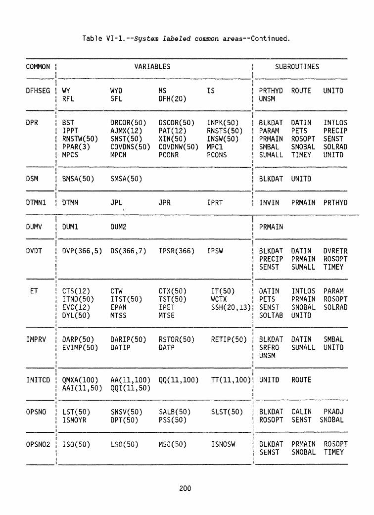
Table VI-1. System labeled common areas--Continued.
COMMON
DFHSEG
DPR
DSM
DTMN1
DUMV
DVDT
ET
IMPRV
INITCD
OPSNO
OPSN02
VARIABLES
WY RFL
BST IPPT RNSTW(50) PPAR(3) MPCS
BMSA(50)
DTMN
DUM1
DVP(356,5)
CTS(12) ITND(50) EVC(12) DYL(50)
DARP(50) EVIMP(SO)
QMXA(IOO) AAI(11,50)
LST(50) ISNOYR
ISO(50)
WYD SFL
DRCOR(50) AJMX(12) SNST(50) COVDNS(50) MPCN
SMSA(50)
JPL
DUM2
DS(356,7)
CTW ITST(50) EPAN MTSS
DARIP(50) DATIP
AA(ll.lOO) QQKU.50)
SNSV(50) DPT(50)
ISO (50)
NS DFH(20)
DSCOR(50) PAT (12) XIN(50) COVDNW(SO) PCONR
JPR
IPSR(366)
CTX(50) TST(50) IPET MTSE
RSTOR(50^> DATP
QQ(11,100)
SALB(50) PSS(50)
MSO(50)
IS
INPK(50) RNSTS(BO) INSW(50) MPC1 PCONS
IPRT
IPSW
IT(50)WCTX SSH(20,13)
RETIP(50)
TT(11,100)
SLST(50)
ISNOSW
SUBROUTINES
PRTHYD UNSM
BLKDAT PARAM PRMAIN SMBAL SUMALL
BLKDAT
INVIN
ROUTE
DATIN PETS ROSOPT SNOBAL TIMEY
UNITD
PRMAIN
UNITD
INTLOS PRECIP SENST SOLRAD UNITD
PRTHYD
RRMAIN
BLKDAT PRECIP SENST
DATIN PETS SENST SOLTAB
BLKDAT SRFRO UNSM
UNITD
BLKDAT ROSOPT
BLKDAT SENST
DATIN PRMAIN SUMALL
INTLOS PRMAIN SNOBAL UNITD
DATIN SUMALL
ROUTE
CALIN SENST
PRMAIN SNOBAL
DVRETR ROSOPT TIMEY
PARAM ROSOPT SOLRAD
SMBAL UNITD
PKADJ SNOBAL
ROSOPT TIMEY
200

Table VI-1. Si/stem labeled common areas Continued.
COMMON
OPT
PCRCHA
PLOT
QSOUT
RD
SED
SENT
VARIABLES
IOPT IPUN1 ISSOL MFS NPRNT IOBS TESTNO(SO)
UPA(50,3) RITEA(50) PROUTA(IOO) THRESA(IOO) DTDXMA(IOO) ALPIA(IOO) ALPIA(50) OFIPA(50) KFA(50)
PRPRO(366) IDPLB PLMN
QSWY QSQS
IRD(50) RDM(12) RDB
OFLT(50) PQ(50)
IWSW2 NV
IOSW IPUN2 ISTMP INIT IWSW OBF(IO) IDOUT
PCRIDA(IOO) UPSWA(BO) NXSA(IOO) DXA(IOO) DTOSA(IOO) CMIA(IOO) ALPI1A(50) D50A(50) MMA(50)
PRORO(366) IMPLE IPLTYP
QSMO QSID
NRD PARS RDP
SEDSG
NOBF XX(20)
IPOP1 IPUN3 LCP(20) NYRI ISEN IOBF IUOUT
RBA(50) TYPEA(50) NDELSA(IOO) DTMA(IOO) DXDTA(IOO) ALPRA(IOO) CMIA(50) KRA(50) ENA(50)
I PLOT IDPLE
QSDY QSRPD
RAD(20,13) PARW RDMX
TSUW(50)
NMOBF XOPT(20)
IPOP2 IPUN4 MFN NDOP ISIM IOBSW
LBA(50) PRTINA(IOO) ODELSA(IOO) DTSA(IOO) DTDXA(IOO) CMPA(IOO) CMI1A(50) HCA(50)
IMPLB PLMX
QSIO
RDC(12) MRDC COSSL(20)
PSED(50)
NDSN
SUBROUTINES
BLKDAT DVRETR PARAM ROSOPT SENST SUMALL TIMEY
INVIN UNITD
DATIN ROSOPT SUMALL
PRTHYD
DATIN SOLTAB
BLKDAT PRMAIN SUMALL
BLKDAT PARAM SENST
COROPT INVIN PKADJ ROUTE SOLRAD SUMUNT UNITD
PARAM UVPLOT
DVPLOT ROUTE
ROUTE
PARAM SUMALL
INVIN ROSOPT SUMUNT
COROPT ROSOPT SUMALL
DATIN OPINIT PRMAIN SENMAT STATS TEMP UVPLOT
ROUTE
PRMAIN SENST
UNITD
SOLRAD
ROUTE SENST UNITD
OPINIT SENMAT
201

Table VI-1. System labeled common areas Continued.
COMMON
SENT1
SENT12
SENT13
SENT14
SENT15
SENT16
SENT17
SENT18
SENT22
SIZE
SM
VARIABLES
XXDEV(20,50)XXAVE(20) NVAR(20) NDVR(20,50) SMVOPT(366) OBSRUN(366) NTRY IPRIOR H(60) CX(20) IQ IR
PINC ILOPL(IOO) ASENS(366,20) ZINV(20,20) OBFOPT VBIN(20,20) G(60) P(20) IP ZINFC(20,20)
PHI(IO)
ITRANS
OFSPR(IO)
TSM(50)
NREC
IOBSWK
ISTAT
IPTEMP
BYW LMO NMO STAIDC(32) IMO
AET(50) ISOIL(SO) SCT(50) SRO(50) SC1(50)
EWY LYR NYR STAIDP(8,5) IDY
ENFIL(SO) RECHR(SO) SLP(50) SRX(50)
IDS NDTY PARMCA(IO) TITL(18) IDUM
EXCS(50) REMX(50) SMAV(50) SCX(50)
IDUS(IO) NOY(12) STATCA(IO) IWY
ICOV(50) SAS SMAX(50) SCN(50)
SUBROUTINES
COROPT ROSOPT
ROSOPT
COROPT ROSOPT
ROSOPT
BLKDAT
COROPT SENST
ROSOPT
DATIN
ROSOPT
BLKDAT DVRETR PRECIP ROSOPT SNOBAL SUNALL UNITD
DATIN RESVRD SMBAL SUMALL
OPINIT SENMAT
SENST
DATIN SENMAT
SUMALL
ROSOPT
ROSOPT SUMALL
SENST
SUMALL
SENST
DATIN INVIN PRMAIN ROUTE SOLRAD TEMP UVPLOT
PARAM ROSOPT SNOBAL UNITD
PARAM SENST
OPINIT SENST
SENST
SENMAT
SUMUNT
DVPLOT PETS PRTHYD SENST STATS TIMEY UVRET
PRECIP SENST SRFRO UNSM
202

Table VI-1. System labeled common areas Continued.
COMMON
SNO
SNOP
SWITCH
UNITRF
UNSS
UPR
UVRT
VOL
WX
ALB(50) IPS1 PKDEF(50) TCALC50) DENI
NSWC50) RMXM
ISBAS ISUN
UPE(1440) TLAT(1440)
UINF(50,96)
IMPERV(SO)
VARIABLES
ANSW IPS2 PWEQV(SO) TRNCF(50) DENMX
PRMX(50) PKAD(50)
ISSRO
INQC1440) QA(1440)
UNBAS(50,
PERV(50)
EAIR PACT(50) SMLT(50) FWCAP SETCON
PSN(50) CECN(12)
ISX1
INS(144Q) TA(1440)
96)CDA(50)
UPCOR(50)
FREWT(50) PICE(50) SNEV(50) ISNO DEN(50)
RMXA
ISSR1
QLAT(1440) HA(1440)
PROLST
UVWY(367)
NST OBPK(50) NOFSEG
CSEL TLX(12) TXAJ(50)
BRO(50) ICHG KRU(50)
ELV(50) TMN SA(50)
X(5,50) SIMOPT(3) I SAVE
TLN(12) TMX
OBRO(50) NCRSEG BPK(50)
TIPS TNAJ(50)
SUBROUTINES
BLKOAT DATIN PKADJ ROSOPT SNOBAL
DATIN PKADJ SNOBAL TIMEY
BASFLW PRMAIN SENST UNITD
PRTHYD UNITD
INVIN
DATIN UNITD
BLKDAT INVIN SMBAL UVRET
BLKDAT PARAM ROSOPT SENST UNITD
DATIN SOLRAD
CALIN INTLOS PRECIP SENST SRFRO
INTLOS PRECIP SRFRO
BLKDAT ROSOPT SRFRO
RESVRU ' UVPLOT
ROUTE
INTLOS
DATIN PRMAIN SUMALL
INVIN PRMAIN ROUTE SMBAL UNSM
PARAM SUMALL
CALOSS PARAM PRMAIN SMSAL SUMALL
PARAM SMBAL SUMALL
DATIN ROUTE SUMALL
ROUTE
SUMALL
SUMALL
DVRETR SENST UVPLOT
OPINIT PRTHYD SENMAT SUMUNT UVPLOT
PRMAIN TEMP
203

ATTACHMENT VII
Modifying PRMS Data Retrieval Subroutines
PRMS uses an indexed sequential (ISAM) file structure for input of streamflow and meteorologic data. Daily data are stored 1 water year per record and storm data are stored 1 day per record. Each record has a key which consists of the station identification, WATSTORE parameter and statistic code, and the year, month, and day of the record. The subroutines DVRETR and UVRET read these ISAM file records. Both subroutines are written in PL1.
Some computer systems do not have ISAM file-handling capabilities that are compatible with the AMDAHL computer system, while others may have no ISAM or PL1 capabilities. To run PRMS on these machines, a compatible file struc ture will have to be selected and the subroutines DVRETR and UVRET will have to be modified or rewritten to read the data from the new file structure. This section describes the subroutines DVRETR and UVRET, their input and output requirements, and data specifications to facilitate any necessary modifica tions required for data storage and retrieval.
Subroutine DVRETR is called at the beginning of each water year and retrieves 366 values for each daily data type. The data are entered into arrays which are included in a labeled common area. The daily meteorologic and streamflow data are entered into the array DS (I,J) where J is dimensioned at 366 and represents the water year day. I is dimensioned at seven and indicates the data type as follows:
I Data type
1 Daily discharge2 Daily pan evaporation3 Daily maximum air temperature4 Daily minimum air temperature5 Daily solar radiation6 Daily data user defined7 Daily data user defined
For example, DS (3,15) would be the maximum air temperature value for October 15 of the water year being simulated. The array IDUS indicates which data types need to be retrieved for the model run. The values for IDUS are read in subroutine DATIN, Card Group 1, card 9.
PRMS can use up to five precipitation gages. Daily data for the water year for all precipitation gages are entered into the array DVP (I,J) where J again is dimensioned at 366 and corresponds to the water year day. I is dimensioned at five and corresponds to the precipitation gage. For example, DVP (3,15) is the precipitation at rain gage 3 for October 15 of the water year being simulated. JDS is the number of rain gages and is read in subrou tine DATIN, Card Group 1, card 4 (NDS).
204

For a storm simulation, the array UVWY (366) is read in DVRETR from file unit 11. This file was written in subroutine INVIN and contains a 0,1 or 2 for every day of the water year, indicating the types of storm data available for that day. A "1" indicates precipitation data only are to be retrieved and a "2" indicates that precipitation and discharge data are available.
The labeled common areas required in DVRETR and the variables used in each of them are the following:
Common
DATES OPT
SIZE
UVRT
DVDT
Variable
JDS ISIM
IWYIDUS(IO)PARMCA(IO)
STATCA(IO)
STAIDC(8)
STAIDP(5,2)
UVWY(366)
DS(7,366) DVP(5,366)
Description
Number of precipitation gagesIndicates type of simulation(ISIM=0 is daily only; ISIM >0 is daily
and storm) Water year Data types WATSTORE parameter code correspond!'nq
to IDUS WATSTORE statistic code corresponding
to IDUS Station I.D.'s for IDUS(l) through
IDUS(8) Station I.D.'s for IDUS(9) and IDUS(IO)
for up to five precipitation gages Storm day indicator (0=no storm;
l=storm day, precipitation data only;2=storm day with precipitation anddischarge data)
Daily meteorologic and streamflow data Daily precipitation data
The type specifications necessary when the above common areas are used in a subroutine are as follows:
INTEGERS STATCA, IWY, IMO, IDY,IDUMINTEGER UVWY, BYR, BMO, BDY, EYR, EMO, EDY, TESTNO, BWY, EWY, PARMCA
Subroutine UVRET is called from subroutine INVIN at the beginning of a storm simulation run. Precipitation and discharge data for all storm days specified in Card Group 2 are retrieved and written sequentially to temporary files for later use in the model run. Precipitation data are written to temporary file unit 15 and the discharge data are written to temporary file unit 14. The UVWY array specifying storm days also is created using the storm day information in Card Group 2.
205

The following unformatted Fortran write statement is an example of how the temporary files are written:
WRITE (15) UVDEL, UVSTA, UVPARM, UVSTAT, UVYR, UVMO, UVDY, UVRPD, UVRDG1, UVNROG, IDUM, UVNVAL, (UVDATA(J), J=l, UVNRDG)
where UVDEL is a blank,UVSTA is the station identification from STAIDC or STAIDP,UVPARM is the WATSTORE parameter code from PARMCA,UVSTAT is the WATSTORE statistic code from STATCA,UVYR is the calendar year,UVMO is the month,UVDY is the day,UVRPD is the maximum number of data values possible (for example,for 15-minute-interval data, UVRPD = 96),
UVRDG1 is the starting index of the first data value (for example,for UVRPD = 96 and first data at 0115, then UVRDG1 = 5),
UVNRDG is the number of data values to be written, IDUM is a dummy variable, and UVDATA(O) is the data array.
UVDATA is dimensioned at 1440 to permit the use of 1-minute data.
Labeled commons "SIZE" and "UVRT" are required in subroutine UVRET. The following type declarations and dimensions also should be used.
LOGICAL*! UVDELINTEGERS STATCA, IWY, IMO, IDY, UVYR, UVMO, UVDY, UVRPD, UVRDG1,
UVNRDG, IDUM, UVSTATINTEGER BWY, EWY, PARMCA, UVWY, UVPARM, OWY DIMENSION UVSTA(4), UVDATA (1440)
206

![The history of investigation of salt water inflows into ...€¦ · runoff (428 km3 ) + precipitation (237 km3) – evaporation (184 km3)] is dominated by runoff because precipitation](https://img.dokumen.tips/doc/110x75/5f7cf0ff5aeed811df507c76/the-history-of-investigation-of-salt-water-inflows-into-runoff-428-km3-.jpg)