PRECAUTIONARY REFERENCE POINTS FOR FRASER RIVER

SOCKEYE SALMON ESCAPEMENT GOALS BASED ON

PRODUCTIVITY OF NURSERY LAKES AND

STOCK-RECRUITMENT ANALYSES

by

Karin Marie Bodtker

B.A. Psychology, University of British Columbia 1981

Dipl. Tech., British Columbia Institute of Technology 1989

RESEARCH PROJECT SUBMITTED IN PARTIAL FULFILLMENT OF

THE REQUIREMENTS FOR THE DEGREE OF

MASTER OF RESOURCE MANAGEMENT

in the

School of Resource and Environmental Management

Project No. 279

© Karin Marie Bodtker 2001SIMON FRASER UNIVERSITY

December 2001

All rights reserved. This work may not bereproduced in whole or in part, by photocopy

or other means, without permission of the author.

iii

Abstract

Accurate and precise determination of optimal spawning escapement is crucial to harvest

management of sockeye salmon (Oncorhynchus nerka). Such escapements have been used as

basis for determining biological reference points in the recent move toward implementing

conservation-oriented policies related to the precautionary approach to fisheries management.

Traditionally optimal escapement is estimated from spawner-recruit data, but these data are not

available for all sockeye salmon populations. Recently, several researchers used data on

productivity of rearing lakes to derive estimates of spawning escapement that should maximize

abundance of juvenile sockeye salmon in the lake. However, only one of these studies accounted

for uncertainty and that was quite limited; the rest produced point estimates. Therefore, I developed

a systematic method of estimating optimal escapement for sockeye salmon based on productivity of

nursery lakes that takes uncertainty into account using a Bayesian approach. Compared to estimates

of optimal spawner abundance produced from Bayesian stock-recruitment analyses of Fraser River,

British Columbia sockeye salmon stocks, this method based on lake productivity produced higher

estimates for the optimal abundance of female spawners in all cases except one, and the precision of

estimates from the two methods was similar. I also propose a scheme for determining biological

reference points from estimates of optimal escapement coupled with estimates of productivity at low

abundance for sockeye population aggregates. The operational performance of specific reference

points developed using this approach needs to be comprehensively assessed, alongside a range of

plausible harvest rules using simulation modeling.

iv

Dedication

To my mother, Joyce Bodtker, for everything a mother provides,

To my partner in life, Dan Blondal, for his unending support and encouragement,

To my son, Ari Blondal, for helping me balance my life.

v

Acknowledgments

I thank my supervisory committee, Randall Peterman and Michael Bradford, for their

generous advise, expertise, and patience. I would also like to thank the members of the Fisheries

Research Group for providing much help and many suggestions that improved this work. I owe

special thanks to Brian Pyper, whose ideas were always insightful, Franz Mueter, whose patience

with statistical questions was ever-present, and Brice MacGregor, who always fielded my questions

with enthusiasm and whose comments on a draft version of this paper were invaluable.

For providing data and technical support, I thank Ken Shortreed, Jeremy Hume, Michael

Bradford, and Jeff Grout (Fisheries and Oceans Canada).

This research was funded by Graduate Fellowships, an NSERC Post-graduate Scholarship,

and Research Assistantships from an NSERC Strategic Projects Grant (via Randall Peterman).

vi

Table of Contents

Approval ............................................................................................................................... ii

Abstract................................................................................................................................. iii

Dedication............................................................................................................................. iv

Acknowledgments.................................................................................................................. v

Table of Contents................................................................................................................... vi

List of Tables......................................................................................................................... viii

List of Figures........................................................................................................................ ix

Chapter 1:

Optimal escapement based on lake productivity and stock-recruitment analyses..........1

Introduction...........................................................................................................................1

Methods ................................................................................................................................4

Fraser River sockeye salmon rearing lakes........................................................................5

Habitat-based estimates of optimal escapement (the Bayesian PR method)........................5

Step 1........................................................................................................................6

Step 2........................................................................................................................8

Step 3........................................................................................................................9

Bayesian stock-recruitment estimates of optimal escapement ...........................................11

Results ................................................................................................................................14

Sensitivity analyses.........................................................................................................15

Exclusion of data from Babine Lake..........................................................................15

Additional years of photosynthetic rate or smolt weight data......................................15

Inaccurate photosynthetic rate or smolt weight input data...........................................16

Number of discrete parameter values explored..........................................................17

Discussion............................................................................................................................17

Comparison of estimates of optimal escapement..............................................................18

vii

Utility of the Bayesian PR method...................................................................................22

Comparison of the Bayesian PR method with the PR and EV models ..............................24

Improving the Bayesian PR method and its application....................................................26

Chapter 2:

Developing biological reference points based on estimates of optimal escapement .....29

Introduction.........................................................................................................................29

Methods ..............................................................................................................................35

Results ................................................................................................................................37

Discussion............................................................................................................................38

Using probability distributions as estimates......................................................................39

Implementation of biological reference points for sockeye salmon escapement goals.........40

Conclusions ........................................................................................................................42

References...........................................................................................................................62

Appendix A:

A Bayesian approach to parameter estimation for linear relationships.....................................67

Appendix B:

Photosynthetic rate and weight per smolt data for Fraser River sockeye salmon.....................69

Appendix C:

Photosynthetic rate (PR) for Early and Late Stuart sockeye salmon stocks.............................71

viii

List of Tables

Table 1. Physical characteristics and trophic status of sockeye salmon nursery lakes in theFraser River drainage basin in British Columbia where data on photosynthetic rates(PR) are available...........................................................................................................44

Table 2. Estimates of photosynthetic rate and weight per smolt used in the application of theBayesian PR method for each of six Fraser River, BC nursery lakes (#1-6) and twoFraser River sockeye stocks (#7-8)................................................................................45

Table 3. Range of observed spawner abundances in S-R data (in units of effective femalespawners, EFS) and estimates of optimal escapement, SMAX, from the PR model ofShortreed et al. (2000), the Bayesian PR method, S-R, and S-J analyses for six BCsockeye nursery lakes and two sockeye stocks...............................................................46

Table 4. Results of sensitivity analysis to determine the effects of inaccurate input data forphotosynthetic rate (PR) or weight per smolt (W) on estimates of optimal escapement,SMAX, produced by the Bayesian PR method. ..............................................................47

ix

List of Figures

Figure 1. Fraser River watershed with major sockeye salmon nursery lakes identified.............48

Figure 2. Conceptual diagram of the 3 steps of the Bayesian PR method................................49

Figure 3. Relationship between maximum observed juvenile sockeye salmon biomass andtotal seasonal photosynthetic rate (PR) in log-log space...................................................50

Figure 4. Estimates of effective female spawners and estimates of smolt abundance at peaksmolt productivity for five BC lakes. ...............................................................................51

Figure 5. Observed stock and recruit data, maximum likelihood estimates for the Rickercurve, posterior probability density functions (pdf) for estimates of the escapement tomaximize recruits, MAXS , from the Bayesian PR method and the S-R analysis or the S-Janalysis of 8 Fraser River sockeye salmon aggregates .....................................................52

Figure 6. Changes in the precision of MAXS estimates from the Bayesian PR method for PittLake with additional years of photosynthetic rate (PR) and weight per smolt (W) inputdata ...............................................................................................................................54

Figure 7. Cumulative probability functions comparing three estimates of the escapement tomaximize recruits, MAXS , for Pitt Lake sockeye salmon calculated using the BayesianPR method and three different input distributions for photosynthetic rate (PR). .................56

Figure 8. Cumulative probability functions comparing three estimates of the escapement tomaximize recruits, MAXS , for Chilko Lake sockeye salmon calculated using theBayesian PR method and three different input distributions for smolt weight at highdensity ( MAXW )..............................................................................................................57

Figure 9. Ratio of equilMSY SS , estimated using the Ricker stock-recruitment model, as a

function of the Ricker a parameter (recruits per spawner at low abundance). ...................58

Figure 10. Provisional estimates of limit reference points (LRP), as probability densityfunctions (pdf), determined from two different combinations of estimates of optimalescapement and sockeye salmon productivity at low abundance for 7 Fraser Riversockeye salmon aggregates.............................................................................................59

Figure 11. Provisional estimates of limit reference points (LRP), as probability densityfunctions (pdf), determined from three different combinations of estimates of optimalescapement and sockeye salmon productivity at low abundance for the Quesnel Lakesockeye salmon aggregate. .............................................................................................61

1

Chapter 1: Optimal escapement based on lake productivity and stock-

recruitment analyses

Introduction

Over the last few years, Pacific fisheries management agencies have developed new

management policies that focus on conservation of wild salmon (Oncorhynchus spp.) stocks. Each

agency has recognized the need to define sets of escapement goals (i.e. numbers of adult recruits

allowed past the fishery to spawn) to meet different objectives, depending on the status of the stocks.

'Optimal' spawning escapement based on maximum sustainable yield (MSY), traditionally used in

harvest management, is becoming a basis for calculating other escapement goals that represent more

conservation-oriented policy targets (e.g., minimum and target levels of abundance might be calculated

as a function of 'optimal' spawning escapement). 'Optimal' escapement goals are termed such because

both lower and higher escapements have negative consequences such as reduced economic returns

and/or potentially unacceptable adverse ecological consequences.

Historically, stock-recruitment analyses and habitat-based models have been used to estimate

optimal escapements of salmon stocks and each method has strengths and weaknesses. Estimates

based on stock-recruitment analyses can be inaccurate and imprecise due to high variability in stock-

recruit data and low contrast in spawner abundances (Hilborn and Walters 1992). Habitat-based

models, usually based on freshwater habitat (e.g., Bradford et al. 2000a for coho salmon), may also

produce inaccurate and imprecise estimates because they rely on indirect indices of the capacity of the

habitat to produce fish. However, habitat-based models can be used to generate estimates of optimal

escapement where stock-recruit data are nonexistent or of poor quality. While stock-recruit data series

2

gathered over decades are required to support stock-recruitment analyses, a relatively short-term study

or analysis might be sufficient to create a habitat-based model.

For sockeye salmon, it is possible to estimate the quality and quantity of their freshwater habitat

from lake productivity because many sockeye salmon rely on lakes for their juvenile nursery. Koenings

and Burkett (1987) found good correlations between euphotic volume (EV) and both total abundance

and biomass of sockeye salmon smolts (i.e. juvenile salmon in the stage of migration to the sea), in

oligotrophic lakes in Alaska. Euphotic volume, calculated from lake surface area (km2) and euphotic

zone depth (Koenings and Burkett 1987), is an index of lake productivity. EV is dependent on lake

clarity and Hume et al. (1996) found that because British Columbia (BC) sockeye lakes had a smaller

range of clarity than the Alaskan sockeye lakes, EV was inappropriate for use as an index of lake

productivity in BC. Therefore, they adapted the relationships of the EV model to use photosynthetic rate

(PR), a more direct measure of lake productivity. Hume et al. (1996) and Shortreed et al. (2000)

developed the PR model from this adaptation of the EV model. Both models used a correlation

between EV or PR and juvenile sockeye salmon abundance to estimate the maximum capacity of a

nursery lake to produce smolts, in units of smolt biomass and numbers. A generally applicable average

of spawner-to-smolt survival rate for sockeye salmon (Koenings and Kyle 1997) was then used in the

EV model to backcalculate spawner abundances required to achieve those smolt maxima (Koenings

and Kyle 1997). In the PR model, optimal spawner escapement was equated with the number of

'spawners per PR unit' that maximized adult returns (Hume et al. 1996; Shortreed et al. 2000), based

on data from Koenings and Burkett (1987).

3

While both the EV and the PR models have been used to estimate optimal spawner

abundances, neither model takes uncertainty into account. Accounting for uncertainty is important for

conservation because biased expectations of productivity based on point estimates may result in

overexploitation of stocks (e.g., Garcia 2000). Also, uncertainty needs to be accounted for in habitat-

based models and stock-recruitment models for researchers to compare precision of estimates of

optimal spawner abundance generated by these models.

The objectives of this study were to: 1) develop a systematic method of estimating optimal

spawner abundance for Fraser River, BC sockeye salmon stocks based on the productivity of their

nursery lakes that explicitly takes uncertainty into account, 2) apply the method to Fraser River sockeye

salmon stocks, and 3) compare these habitat-based estimates with optimal escapement estimated

independently from standard stock-recruitment analyses. I refer to the habitat-based method I

developed as the Bayesian PR method because I used Bayesian statistical methods and represented

parameters and estimates of variables with probability distributions.

In theory, estimates of optimal escapement from two independent sources of information could

be combined to produce a single estimate that may be more precise simply because more information

has been applied to the problem. Geiger and Koenings (1991) estimated optimal escapement for

sockeye salmon stocks by combining estimates of the capacity of their freshwater habitat with stock-

recruit data, using a Bayesian approach to take uncertainty into account. However, they used subjective

estimates of capacity of freshwater habitat based on expert opinion instead of data and inadvertently

combined contradictory information in a way that led to high confidence for specific estimates of optimal

escapement that were unwarranted by both the information on habitat capacity and the stock-recruit

4

data (Adkison and Peterman 1996). I chose not to combine estimates of optimal escapement generated

by the Bayesian PR method with independent estimates from stock-recruitment analyses but rather

chose to contrast the results of the two methods.

Methods

I estimated optimal escapement based on the Bayesian PR method for six sockeye salmon

nursery lakes (Chilko, Francois, Fraser, Pitt, Quesnel, and Shuswap Lakes) and two stocks (the Early

Stuart and Late Stuart stocks) of the Fraser River system in British Columbia. 'Optimal' escapement

here is the escapement that maximizes annual smolt biomass in the freshwater habitat. For comparison, I

also estimated two other optimal escapements. The first was the escapement that maximizes annual

juvenile (fall fry or smolt) sockeye salmon abundance (JSMAXS

−) based on spawning stock and juvenile

recruitment analysis (referred to here as S-J analysis) for three lakes where juvenile data were available

(Chilko, Quesnel, and Shuswap Lakes). The second was the escapement that maximizes total adult

recruitment (in numbers of fish) (RSMAXS

−) based on standard stock and adult recruitment analysis

(called S-R analysis) for all the lakes and stocks. Note that optimal escapement based on stock-

recruitment analyses usually refers to the escapement that maximizes catch ( MSYS ), rather than the

escapement that maximizes adult recruits ( MAXS ). I use the term optimal escapement in the latter

context, defining it as the escapement that maximizes abundance or biomass (depending on the method)

to make all the 'optimal' estimates comparable. These 'optimal' escapements are to be used as a basis

for estimating target reference points (defining desired abundances) and limit reference points

(abundances that are some small fraction of those optimal escapements and below which the spawning

5

stock should not drop). In each type of analysis I take uncertainty into account explicitly by using

Bayesian statistical methods and representing all parameters and estimates with discretized probability

distributions. Chilko Lake cohorts that would have been affected by lake fertilization experiments (i.e.

brood years 1987-1992; Bradford et al. 2000b) were excluded from all analyses to avoid biasing

estimates of productivity.

Fraser River sockeye salmon rearing lakes

Many lakes in the Fraser River's drainage basin provide nursery habitat for juvenile sockeye

salmon (Figure 1). The nursery lakes of the Fraser River system are ideal for this work because they

have relatively good estimates for abundance of major stocks and for productivity in their nursery lakes

compared to other BC nursery lakes. The sockeye salmon nursery lakes in the Fraser system for which

data appropriate to this study were available are Chilko, Francois, Fraser, Pitt, Quesnel, Shuswap,

Stuart, Takla, and Trembleur, the latter three lakes being occupied by the two Stuart stocks. These

lakes range widely in their characteristics (Table 1). The distances that sockeye salmon cover during

their migrations between these lakes and the ocean range from under 100 to over 1000 km.

Habitat-based estimates of optimal escapement (the Bayesian PR method)

The Bayesian PR method consists of three steps (Figure 2): 1) first, I used lake productivity

(photosynthetic rate) to estimate the maximum sockeye salmon smolt biomass (capacity) that each

nursery lake can produce; 2) then I converted smolt biomass to smolt abundance, using lake-specific

estimates of weight per smolt at high smolt densities; and 3) I estimated the minimal spawner abundance

required to produce those smolts and called this 'optimal' spawner abundance. Empirical relationships

6

provide the basis for estimations in steps 1 and 3, and because both of these relationships were

heteroscedastic, I used natural logarithm transformations. These three steps are detailed below.

Step 1

In step 1, I estimated the maximum capacity of each nursery lake to produce sockeye salmon:

(1) iTOTALeiMAXe PRSB loglog •+= γδ ,

where iMAXSB is the maximum smolt biomass (tonnes year-1) that lake i can produce, δ and γ are the

intercept and slope parameters, respectively, of the empirical relationship between mean photosynthetic

rate (PR) and maximum observed juvenile sockeye salmon biomass, and iTOTALPR is the total seasonal

(May to October) carbon production (tonnes) in lake i. Step 1 was based on a positive empirical

relationship between total seasonal PR and maximum observed juvenile sockeye salmon biomass

(Hume et al. 1996; Shortreed et al. 2000) in 10 rearing-limited nursery lakes (Figure 3). Rearing-limited

means that juvenile sockeye salmon output from these lakes has peaked as a function of poor lacustrine

conditions or fry-food interaction, instead of from limitations caused by the number of spawners or the

amount of spawning area (Koenings and Burkett 1987). Data to calibrate this relationship were from

Figure 32.2b in Shortreed et al. (2000) (K. S. Shortreed, Fisheries and Oceans Canada, Cultus Lake

Laboratory, 4222 Columbia Valley Highway, Cultus Lake, BC, V2R 5B6, Canada, personal

communication). Data were fall fry biomass for Quesnel and Shuswap lakes and smolt biomass for all

other lakes. Smolt biomass data for the six Alaskan Lakes, originally from Koenings and Burkett (1987,

Table 6), were averages of one to three years of biomass observations in rearing-limited lakes. For the

four BC lakes, I used the maximum annual juvenile biomass observed to date and assumed these lakes

were rearing-limited in that year (Hume et al. 1996).

7

I estimated a joint posterior probability distribution for the intercept (δ ) and slope (γ )

parameters (Equation 1) of the relationship between loge (observed juvenile sockeye salmon biomass in

tonnes year-1) and loge (total seasonal PR in tonnes of carbon year-1) (Figure 3), using a Bayesian

approach (Appendix A). I used uniform prior probability distributions for δ and γ , each bounded by

the maximum likelihood estimate (MLE) ± 3 standard errors (SE) and described by 20 grid points of

values and associated probabilities. As a result, the joint posterior probability distribution representing

δ and γ was a 20-by-20 grid of parameter values with corresponding probabilities.

The input to Equation 1 is the mean PR for a lake. PR data are usually available for only a few

years, so that the true value for each lake is uncertain. To characterize the uncertainty in estimates of

iTOTALPR , I used discretized log-normal distributions. Means of those distributions were averages of

available annual estimates for each lake (Table 2), while standard errors were based on the amount of

lake-specific data available and an estimate of within-lake year-to-year variability in TOTALe PRlog

(Appendix B), assumed to be the same across lakes. The range of possible values, defined by

)(log TOTALe PR ± 3 SE, was divided equally into discrete bins and I used 20 grid points and associated

probabilities to represent each input distribution. Means and SEs for the input distributions representing

TOTALPR for the Early and Late Stuart sockeye salmon stocks were calculated (Appendix C) to be

stock-specific rather than lake-specific because juvenile fish from these two stocks rear in three lakes,

sharing one between them. Hence, stock-specific TOTALPR estimates were calculated to describe the

productivity of their respective average freshwater habitats.

8

To apply Equation 1 to each lake, I took an iterative approach. For each lake i, MAXe SBlog

was computed according to Equation 1 using each grid point value in the discrete probability distribution

for iTOTALe PRlog in combination with each pair of parameter values from the grid points of the joint

posterior probability distribution for δ and γ . Thus, I computed a total of 8000 possible values for

MAXe SBlog . The probability associated with each MAXe SBlog value was computed by applying the

multiplication law for the probability of independent events:

(2) )(log)()(log imTOTALekijMAXe PRPPSBP θ= .

Here, )(log ijMAXe SBP is the computed probability for each possible iMAXe SBlog value, for j = 1 to

8000, )( kP θ is the probability associated with a set of δ and γ parameter values, for k = 1 to 400,

and )(log imTOTALe PRP is the probability associated with a iTOTALe PRlog grid point, for m = 1 to 20.

Before proceeding to step 2, I standardized the 8000 probability values associated with

iMAXe SBlog , so that the discrete probabilities summed to one. Then I truncated the array of

iMAXe SBlog values and probabilities at both ends to get the 99% interval and avoid extreme tails and

standardized the truncated array so the discrete probabilities summed to one again. To make further

calculations manageable, I created a discrete distribution with 20 iMAXe SBlog values and associated

probabilities.

Step 2

In step 2, I converted the estimated maximum capacity for each lake from smolt biomass to

smolt abundance:

9

(3)iMAX

iMAXeiMAXe W

SBSN loglog = ,

where iMAXSN is the maximum smolt capacity for lake i, in numbers of smolt, and iMAXW is the lake-

specific weight per smolt (tonnes) at maximum smolt capacity. I described MAXW by discretized log-

normal distributions, which were parameterized the same way as the TOTALPR input to step 1 (Table 2,

Appendix B). I used the iterative approach described in step 1 to combine the two distributions on the

right side of Equation 3, resulting in 400 possible values for iMAXe SNlog each with an associated

probability. Following the same procedure described at the end of step 1, I standardized, truncated,

restandardized and reduced the results of step 2 into a discrete distribution with 20 iMAXe SNlog values

and associated probabilities before proceeding to step 3.

Step 3

In step 3, I estimated the minimal number of female spawners (in units of "effective female

spawners", EFS, or the number of female spawners reduced by prespawning mortality (Pacific Salmon

Commission 1998)) required to yield the maximum smolt abundance in each lake:

(4) iMAXeiMAXe SNEFS loglog •+= λκ ,

where iMAXEFS is the minimum escapement needed to produce iMAXSN smolts and κ and λ are the

intercept and slope parameters, respectively, of the empirical relationship between EFS and smolt

abundances at high smolt density across lakes. The data used to calibrate this relationship were point

estimates of EFS and smolt abundances at the peak of the spawner-to-smolt relationship for sockeye

salmon populations in five BC lakes. These point estimates were derived using a Ricker model, shown

here in the linear form:

10

(5) pqpqqqpqpqe vSbaSR +−=)/(log ,

where Spq is the abundance of spawners (EFS) in brood year p for population q, Rpq is the number of

smolts produced by Spq spawners, and vpq is the stochastic error term, assumed to be normally

distributed with standard deviation qσ (Peterman 1981). First, I calculated MLEs of the Ricker aq and

bq parameters, then I computed the arithmetic mean for each productivity parameter

( )2( 2qqq aa σ+=′ ) to better describe 'average' spawner-to-smolt relationships (Ricker 1997). Next,

point estimates of spawner abundance ( qqMAX bEFS 1= ) and smolt abundance ( qa

qMAX beSN q 1−′= )

at the peak of each Ricker curve were calculated from formulas in Ricker (1997). Finally, using these

point estimates and the same Bayesian approach (Appendix A) and treatment of priors that I described

in step 1, I derived a joint posterior probability distribution for parameters κ and λ (Equation 4) of the

relationship between MAXe EFSlog and MAXe SNlog (Figure 4).

The five time series of EFS and smolt abundance used here included 43 years from Chilko

Lake, 29 years from Cultus Lake, 11 years from Babine Lake prior to enhancement, 9 years from Port

John Lake, and 8 years from Lakelse Lake. Most juveniles (>95%) from all but one of these

populations spend one winter in freshwater and migrate to sea as age-1 smolts, although some age-2

smolts were included in the abundance estimates. The exception is Port John Lake, where most smolts

were age-2 and smolts of ages-1, -2, and -3 were included in the estimates. Data were from Foerster

(1968), Wood et al. (1998), J.M.B. Hume (Fisheries and Oceans Canada, Cultus Lake Laboratory,

4222 Columbia Valley Highway, Cultus Lake, BC, V2R 5B6, Canada, personal communication), and

M.J. Bradford (Fisheries and Oceans Canada and Cooperative Resource Management Institute,

11

School of Resource and Environmental Management, Simon Fraser University, Burnaby, BC, V5A

1S6, Canada, personal communication).

Again, I used the iterative approach described in step 1 to apply Equation 4 and computed

8000 possible MAXe EFSlog values and associated probabilities for each lake. Using the exponential

function, I transformed these estimates to EFS abundance (from loge values). Results were compiled

from the entire 8000-bin distribution of iMAXe SNlog values and standardized probabilities. To describe

the precision of the final distributions, I used an 80% credibility interval (i.e. 90th percentile estimate less

10th percentile estimate) divided by the median. Therefore, lower values of this ratio reflect greater

precision. For graphs, the arrays of 8000 iMAXe SNlog values and standardized probabilities were

truncated to get the 99% interval and then described as 20-bin discrete distributions, each standardized

such that the discrete probabilities summed to one.

Bayesian stock-recruitment estimates of optimal escapement

To allow the results from the Bayesian PR method to be compared with estimates of optimal

escapement based on standard stock-recruitment analysis, I applied a Bayesian approach to the latter

as well (Walters and Ludwig 1994). I used the same Ricker stock-recruitment model form as in

Equation 5, but estimated the spawning escapement that maximizes abundance ( MAXS ) of either total

adult recruitment (S-R analyses) or juveniles at the end of their lake residence (S-J analyses). MAXS is

the most appropriate index from fitting the Ricker model to compare with the escapement that

maximizes smolt biomass in nursery lakes (i.e. derived from the Bayesian PR method). Estimates of EFS

were used in all analyses as an index of total spawners.

12

For the S-R analyses, I used EFS-recruit data (brood years 1949 through 1992) for 11

sockeye salmon populations that rear in 8 lakes (Table 2) in the Fraser River watershed (M.J.

Bradford, personal communication). S-R analysis for the Horsefly and Mitchell populations rearing in

Quesnel Lake was excluded from this study because these data show very little evidence of density

dependence and do not support use of the Ricker model. Most Fraser River sockeye salmon juveniles

migrate to the ocean as smolts after one winter in freshwater (Foerster 1968) and I included only these

"1.x" age-classes in the adult recruit data. I summed wild spawner abundance and spawner abundance

in the Nadina spawning channel for the S-R analysis of the Nadina population that rears in Francois

Lake. Note also that the Pitt Lake population is augmented by a hatchery operation that uses native

brood stock and releases hatchery raised fry each year. I analyzed the spawner-recruit data despite this

'enhancement.' Abundance estimates were summed for populations whose juveniles rear in the same

lake (Table 2, lakes #1-4, 6) and I estimated optimal escapement on a lake-by-lake basis for these

population aggregates, so they were comparable with estimates from the S-J analyses and the Bayesian

PR method. However, stock-specific (as opposed to lake-specific) estimates of optimal escapement

were generated for the Early Stuart and Late Stuart stocks to compare with estimates produced by the

Bayesian PR method for these two stocks.

For S-J analyses, juvenile abundance data were available for Chilko, Quesnel, and Shuswap

Lakes (Hume et al. 1996 and J.M.B. Hume, personal communication). Smolt abundance estimates for

Chilko Lake (brood years 1949 - 1986 and 1993 – 1997) were taken from a counting fence at the

outlet of the lake. Fall fry abundance was estimated from hydroacoustic surveys for Quesnel Lake

13

(brood years 1976, 1977, 1981, 1985-1987, 1989-1991, 1993, 1994, and 1997) and Shuswap Lake

(brood years 1974-1979, 1982, 1983, 1986-1992, 1994, and 1995).

For the Bayesian stock assessments, I also used 'uninformative' priors (Punt and Hilborn 1997).

Upper and lower bounds for the uniform prior probability distributions on a and b (Equation 5) were

defined by their respective MLE ± 3 SE (e.g., )ˆ(3ˆ aSEa ± ). However, I was able to use )ˆ(3ˆ bSEb −

as the lower bound on b for only three analyses (i.e. S-R analysis for Francois Lake and S-J analyses

for Chilko and Shuswap Lakes) without going below the biologically reasonable value of zero (Punt and

Hilborn 1997; Hill and Pyper 1998). For the remainder of the analyses, estimates of )ˆ(3ˆ bSEb − were

negative and biologically unreasonable because they implied a positive slope on the ( ) SSRe vs.log

graph. For such stocks, instead of assuming the stock size could reach infinity, I arbitrarily assumed that

3 times the maximum observed EFS abundance ( OBSMAXEFS , ) was a biologically reasonable maximum

bound for the parameter MAXS , in units of EFS, and set the lower bound on b equal to

)3(1 ,OBSMAXEFS• . As the lower bound on b approaches zero, the precision of MAXS estimates

declines and the upper bound of the MAXS distribution increases. Difficulty in setting a lower bound for

b based on statistical analysis of the S-R data alone implies that these data are not informative about the

b parameter.

A 200-by-200 grid of a and b parameter values and associated probabilities was calculated for

each S-R and S-J analysis using methods outlined by Walters and Ludwig (1994). Because MAXS is

equivalent to 1/b, the posterior probability distribution for MAXS was converted, by inversion, from the

marginal posterior probability distribution for b integrated over all probable a parameter values (Walters

14

and Ludwig 1994). Results describing estimates of MAXS (i.e. percentile and precision estimates) were

calculated from the resulting 200-value discrete marginal posterior probability distributions, but for

graphs distributions were reduced to 20 grid points and standardized such that the discrete probabilities

summed to one.

Results

The spawning escapement required to maximize biomass of juvenile sockeye salmon in nursery

lakes ( MAXS ), as estimated by the base case of the Bayesian PR method, was generally higher than the

spawning escapement required to maximize either total adult sockeye salmon recruits or juvenile

abundance in nursery lakes as estimated by the S-R and S-J analyses, respectively (Table 3, medians).

The only exception was Chilko Lake, where estimates of optimal escapement from the three methods

are similar, but the Bayesian PR method produced the lowest of the three estimates. Estimates of

optimal escapement based on the Bayesian PR method are independent of estimates based on stock-

recruitment analyses for all but three of the examples. Estimates for Chilko, Quesnel and Shuswap

Lakes are not independent because estimates of maximum observed juvenile biomass from these three

lakes were used to help parameterize the Bayesian PR method.

Estimates of optimal escapement from the Bayesian PR method were slightly more precise than

those from S-R analyses and less precise than those from S-J analyses, with the exception of Francois

Lake (Table 3, Figure 5). Precision of estimates of optimal escapement, MAXS , based on S-R or S-J

analyses varied greatly among lakes and was best when the observed data showed clear evidence of

density dependence (e.g., S-R analyses for Francois and Pitt Lakes or any of the S-J analyses, Figure

5). These are the few cases where posterior probability distributions for MAXS were largely contained

15

within the range of historical observations. The precision of estimates of MAXS based on the Bayesian

PR method was relatively consistent among lakes and improved as the median value for MAXS

decreased. Although all the posterior distributions for MAXS were skewed, those resulting from S-R

analyses were often more skewed to the right (i.e. had a longer tail at high escapements) than those

resulting from the Bayesian PR method. Thus, S-R data can be poor at defining the upper limit for

MAXS (e.g., Early Stuart S-R analysis, Figure 5).

Sensitivity analyses

Exclusion of data from Babine Lake

I examined the sensitivity of results of the Bayesian PR method to the inclusion of Babine Lake

data in the calibration of both of the predictive relationships (used in steps 1 and 3) because my

assumption that Babine Lake was producing smolts at its peak capacity may not be valid. Abundance of

juvenile sockeye salmon in Babine lake was limited by the capacity of its spawning grounds prior to

enhancement with spawning channels in 1965 and it may still be, despite enhancement (West and

Mason 1987). When I removed the Babine data point from each of the predictive relationships (Figures

3 and 4) and repeated the Bayesian PR analyses, the medians of the resulting probability distributions

for MAXS were 10 to 20 percent higher (Table 3).

Additional years of photosynthetic rate or smolt weight data

The base case analyses of the Bayesian PR method were mostly based on few years of

photosynthetic rate (PR) and smolt weight ( MAXW ) data for each lake, so I asked how the precision of

the MAXS estimates would change with additional years of input data. To do this, I simulated the effect

of acquiring additional years of PR or MAXW data by increasing n in Equations B1 and B2, which

16

narrowed the input distributions. As expected, increasing the data available improved the precision of

estimates of MAXS (Figure 6), but not by much. The greatest relative gains in precision were made when

available data were doubled from one to two years and relative gains in precision diminished as more

years of data were added.

Inaccurate photosynthetic rate or smolt weight input data

I also examined how inaccurate input data for PR or MAXW might affect estimates of MAXS

produced by the Bayesian PR method. When few data are available, estimates of the means for PR and

MAXW could be inaccurate. I adjusted the base case mean of the input distribution for PR or MAXW by

± 2 SE (leaving the standard errors of the input distributions at their base case values). Since the

method relies on linear relationships, changes in MAXS were proportional to changes in the inputs (Table

4, Figures 7-8). The effect of using potentially inaccurate inputs for PR and MAXW was substantial.

However, the medians of these adjusted MAXS estimates from the sensitivity analyses were still within

the 80% credibility interval of MAXS values estimated by the base case Bayesian PR method, with the

exception of the results from the PR± 2 SE analyses for Pitt Lake (Figure 7), which were within the

99% credibility interval of base case MAXS . The relative adjustment to the mean PR for Pitt Lake was

the largest (amongst the lakes) because the SE estimated for Pitt Lake PR was large, as only one year

of PR data was available. The precision of the estimates of MAXS changed very little as a result of

changes to the mean input values for PR or MAXW .

17

Number of discrete parameter values explored

Results of Bayesian analyses can potentially be affected by the number of discrete parameter

values used in calculations (as opposed to assuming a continuous range of values) (Walters and Ludwig

1994). Therefore, to examine the sensitivity of my results for the Bayesian PR method to this potential

bias, I compared results using 20 (base case), 40, and 100 discrete parameter values for the two input

distributions (PR and MAXW ) and for the intermediate results calculated by steps 1 and 2. I also

compared results using a 20-by-20 grid (base case) and a 40-by-40 grid to define the joint posterior

probability distributions for parameters of the two predictive relationships, combined with trials of 20

and 40 discrete parameter values for the input distributions (PR and MAXW ) and the intermediate results.

I found very small differences in the probability distributions for MAXS , indicating that the discretized

ranges of parameter values provided a close approximation to the true probability distributions.

Discussion

Estimates of optimal escapement from habitat-based analyses were generally higher than

estimates of optimal escapement based on stock-recruitment analyses. Contradictory results are not

surprising because the methods analyze different sets of processes. Also, because the results are

contradictory, they cannot be combined to estimate optimal escapement with greater precision.

However, because the differences were generally in the same direction for most sockeye salmon stocks,

they may be indicative of general mechanisms acting to different degrees in each lake. In addition, the

lake-specific differences between estimates can be examined to learn more about individual systems.

While the precision of estimates from the different analyses did not differ greatly overall, RSMAXS

−

18

distributions from the standard adult S-R analyses were often more skewed to the right than those from

the Bayesian PR method, suggesting that habitat-based analyses may be more useful than S-R analyses

in defining an upper limit for optimal escapement when the range of S-R data is limited.

Comparison of estimates of optimal escapement

There are several plausible explanations of my finding that estimates of optimal escapement,

MAXS , from the Bayesian PR method were generally higher than estimates based on S-R or S-J

analysis. First, the range of historically observed escapements is often below the range of RSMAXS

−

estimates (Figure 5). If there is substantial measurement error in the historical estimates of spawner

abundance and the range of these estimates is small, S-R analysis will always underestimate optimum

stock size (Hilborn and Walters 1992, p. 287). If this were the case, I would expect PR-based

estimates of MAXS to be greater than S-R based estimates and I would expect estimates from the two

methods to converge when the range of spawner abundance estimates was large. However, spawner

abundance estimates for Fraser Lake span only 2 orders of magnitude and the MAXS estimates from the

two methods overlap considerably. Additional lakes where PR-based and S-R based MAXS estimates

overlap (Chilko, Quesnel, and Shuswap Lakes) have estimates of spawner abundance spanning 3 to 5

orders of magnitude, but these are also the lakes included in the calibration of the Bayesian PR method,

so MAXS estimates from the two methods are not independent. On the other hand, spawner abundance

estimates for Francois Lake cover 5 orders of magnitude, suggesting that RSMAXS

− should be relatively

unbiased, but S-R based and PR-based MAXS estimates still differ by an order of magnitude. Thus, while

bias due to measurement error and limited contrast in spawner abundance estimates is certainly an issue,

it alone cannot explain the results.

19

Second, MAXS estimated by the Bayesian PR method is the stock size that maximizes smolt

abundance, while MAXS estimated by my S-R analyses is the stock size that maximizes total adult

recruits. If marine abundance of a given population influences its reproductive fitness as adult sockeye

salmon or their survival rate during the smolt-to-adult life stages (e.g., Peterman 1982; Peterman 1984;

Bugaev et al. 2001), estimates of RSMAXS

− would be lower than those from the Bayesian PR method.

However, it is hard to imagine that either of these first two explanations could account for the large

discrepancies between estimates of MAXS illustrated by the Francois, Pitt, and Late Stuart examples

(Figure 5).

Third, when I used the Bayesian PR method, I generalized from the lakes for which rearing-

limited data were available (i.e. those in Figure 3) and assumed that other lakes were similar. If these

other lakes are different, results from the Bayesian PR method might reflect a capacity that cannot

actually be achieved. There are several plausible mechanisms, not necessarily independent of each

other, that would limit the abundance of sockeye salmon smolts produced in nursery lakes and cause

MAXS estimates from S-R analyses to be significantly lower than estimates based on the Bayesian PR

method. For instance, Shortreed et al. (2000) noted mechanisms such as limited spawning habitat,

predator and competitor populations, thermal regimes that limit juvenile sockeye salmon feeding

territory, and predation-resistant plankton community structures, all of which can affect a lake's ability to

produce sockeye salmon. These mechanisms, examined in more detail below, are accounted for in

habitat-based analyses (i.e. EV and PR models and Bayesian PR method) only to the extent that they

may be acting in some of the lakes used to parameterize the models.

20

Some examples of these mechanisms illustrate the potential caveats of using any method based

on photosynthetic rate. Limited spawning habitat may mean that the capacity of a lake to produce

sockeye salmon smolts estimated based on PR will be under-utilized. For instance, the spawning habitat

around Francois Lake has been enhanced with an artificial spawning channel. Total natural and

enhanced spawning ground capacity was estimated at 50 thousand spawners (Rosberg et al. 1986 as

cited in Shortreed et al. 1996), or about 26 thousand EFS, which is a full order of magnitude below the

MAXS estimate from the Bayesian PR method (320-750 thousand EFS, Table 3). In contrast, S-R

based estimates optimal escapement (median of 13 thousand EFS, Table 3) are about half of the

estimated spawning ground capacity. This example illustrates that estimates of optimal escapement

based on the Bayesian PR method in the absence of other stock size information or estimates of

spawning ground capacity could be quite unrealistic.

In cases where competitors or predators of juvenile sockeye salmon reduce the maximum

achievable abundance of sockeye salmon juveniles in a lake, the Bayesian PR method may overestimate

the capacity of the lake to produce sockeye salmon smolts. However, while other planktivores are

present in most of the study lakes (e.g., kokanee or smelt), they are not always competitors with

juvenile sockeye salmon (Diewert and Henderson 1992). In addition, significant populations of potential

predators of sockeye salmon juveniles may be present in the lakes (e.g., juvenile chinook salmon or

rainbow trout), but sockeye salmon are not always a major component in their diet (Diewert and

Henderson 1992). Because the food webs are complex and unique among lakes, experiments may be

required to estimate optimal escapement for these systems independently.

21

Another mechanism that would limit abundance of sockeye salmon juveniles in a nursery lake is

thermal stratification resulting in an epilimnion warm enough to restrict foraging fry in their use of this

productive area of the lake. Evidence suggests this may be the case in Shuswap Lake (Hume et al.

1996) and such an effect would be consistent with the density dependence evident in the Shuswap fall

fry data (Figure 5). This could be related to my results showing that the PR-based median estimate of

MAXS is approximately three times larger than the S-J based median estimate of MAXS (Table 3) for that

lake. In addition, the S-R data for the Shuswap aggregate show total adult returns decreasing above

one million EFS (Figure 5), which corresponds more closely to the S-J based estimate of MAXS , even

though the Ricker S-R analysis estimates a much higher MAXS (Table 3).

While the Bayesian PR method uses empirical data to relate primary lake productivity to

maximum numbers of sockeye salmon juveniles, there is no evidence to suggest that nursery lakes can

produce sockeye salmon sustainably at maximum capacities estimated by the Bayesian PR method.

Maximum observed juvenile biomass data used to develop the Bayesian PR method were based on

three years of observations, at most, for any one lake and were single occurrences for the five BC

lakes. Plankton community structure and productivity are complex and may not be able to sustain high

grazing pressure from sockeye salmon fry year after year. In addition, some evidence suggests that high

grazing pressure from sockeye salmon fry may result in predation-resistant plankton communities (i.e.

predominantly smaller zooplankton species) and subsequent reductions in juvenile sockeye salmon

abundance (Koenings and Kyle 1997). On the other hand, repeated high escapements that maintain

high levels of nutrient loading from carcasses may be necessary to bolster salmon productivity in the long

term (Schmidt et al. 1998). More research is needed to explore the effects of repeated high

22

escapements and heavy grazing pressure of large juvenile sockeye salmon populations (i.e. maximum

capacities estimated by the PR method).

The only results that are contrary to what we might expect from the above discussions are those

from Chilko Lake because MAXS estimated by the Bayesian PR method was slightly smaller than MAXS

estimated by either the S-R and the S-J analyses (Table 3). However, the distributions for MAXS from

all three analyses overlap considerably (Figure 5). The mode of the distribution of the MAXS estimate

based on the Bayesian PR method for Chilko Lake corresponds well to the observed spawner

abundance that produced the greatest number of smolts (Figure 5) partly because Chilko data were

used to calibrate the Bayesian PR method.

Comparing habitat-based estimates of optimal escapement (i.e. from the EV or PR models or

the Bayesian PR method) with those based on S-J or S-R analyses suggests that mechanisms limiting

the abundance of juvenile sockeye salmon within nursery lakes are at play to different degrees in

different lakes. Comparing MAXS estimates cannot differentiate between hypotheses but can support the

need for additional investigation of specific mechanisms in specific lakes.

Utility of the Bayesian PR method

From a management perspective, there is great utility for the Bayesian PR method, despite its

current limitations. If estimates of optimal escapement based on the Bayesian PR method are to be used

in setting escapement goals, each of the mechanisms which can limit the abundance of sockeye salmon

in nursery lakes needs to be considered. This is especially true if the Bayesian PR method is used as a

stand-alone method of assessment. There are several sockeye salmon lakes on the west coast of North

America without stock and recruit data to support adult S-R analyses (or where stock and recruit data

23

are of dubious quality). After PR data are collected over one or two growing seasons in those nursery

lakes, smolt abundance at maximum capacity, optimal escapement, and the uncertainty around them can

be estimated. The Bayesian PR method could also be applied to lakes and reservoirs that kokanee

(land-locked sockeye salmon) inhabit, to estimate the maximum annual production of kokanee biomass.

The Bayesian PR method can also be used in combination with stock-recruitment analyses to

identify systems that might benefit from enhancement and quantify the potential benefits. For example,

this study suggests that if spawning ground capacity around Francois Lake existed for 300-750

thousand EFS, the lake could rear 31-48 million smolts (inter-quartile range) and, assuming 5% ocean

survival, result in 1.5-2.5 million adults, or 5-8 times observed abundances. Such estimates of projected

potential can help inform benefit-cost analyses and management decisions about whether to proceed

with enhancement or costly research (e.g., to study the abundance and diet of sockeye salmon

competitors and predators or plankton community structure).

When S-R data show little or no evidence of density dependence, sockeye salmon populations

are suspected of being recruitment-limited (e.g., Early Stuart, Late Stuart, and Fraser Lake examples,

Figure 5). In these cases, estimates of MAXS from the Bayesian PR method, such as most of those

reported here, can support calls for larger escapements for two reasons. First, they give managers

confidence that nursery lakes can support the additional sockeye salmon fry produced by higher

spawning escapements, especially when S-R analyses provide no such evidence. Second, additional

data from subsequent larger escapements can be used to recalibrate relationships and refine the

Bayesian PR method. Specifically, data from BC nursery lakes where empirical evidence strongly

24

suggests that sockeye salmon juveniles are rearing-limited may reduce the uncertainty implicit in the

Bayesian PR method.

The utility of the Bayesian PR method discussed thus far has been implicitly related to harvest

management, in terms of setting escapement goals for healthy stocks that can support harvest, assessing

enhancement potential to increase harvest, and providing estimates of the maximum capacity of nursery

lakes independent from S-R data, again to maximize harvest. Chapter two discusses the utility of this

method in the context of conservation-oriented policies and develops a scheme to quantify biological

reference points based on estimates of optimal escapement from either the Bayesian PR method or

Bayesian stock-recruitment analyses.

Comparison of the Bayesian PR method with the PR and EV models

The most significant difference between the Bayesian PR method developed here and the PR

model of Shortreed et al. (2000) is that the first accounts for uncertainty. However, because these

methods used different data to calibrate the two predictive relationships and different estimates for smolt

weight as input, estimates of maximum smolt abundance and optimal escapement differ for a given lake.

The Bayesian PR method produced median estimates of MAXS that were higher than, or nearly the same

as, the point estimates produced by the PR model (Shortreed at al. 2000), with the exception of

Francois Lake (Table 3). While lake-specific mean PR values were identical for each method, they

estimated different quantities for the maximum capacity of smolt biomass in a given nursery lake because

the Bayesian PR method included four BC lakes in the calibration of the PR versus maximum smolt

biomass relationship and its parameters were estimated in loge space. As a result, for large lakes with

25

high total seasonal PR, the Bayesian PR method estimated higher maximum capacities of juvenile

sockeye salmon biomass (Figure 3, dotted line) than did the PR model (Figure 3, dashed line).

Differences between the Shortreed et al. (2000) PR model and my Bayesian PR method in

estimates for smolt weight used as input and smolts/EFS had a greater effect on the results than

differences in the calibration of the first predictive relationship. The PR model used a point estimate of

4.5 g per smolt for all lakes, while the Bayesian PR method used lake-specific estimates whose means

range from 2.7 to 9.7 g (Table 2). Also, the Bayesian PR method consistently estimated that more EFS

were required to produce the same number of smolts than did the PR model. The average smolts/EFS

ratio used by the base case Bayesian PR method varied from 51 to 78 smolts/EFS over the range of

observed smolt abundances (Figure 4, dotted line), based on analysis of data from 5 BC lakes. When

the Babine Lake datum was removed from the model fitting for sensitivity analysis, the slope became

almost constant at 57 to 59 smolts produced per EFS. The PR model (Shortreed at al. 2000) used a

constant estimate of 108 smolts/EFS (Figure 4, dashed line), while the EV model used a smolts/EFS

ratio of 54 (Koenings and Kyle 1997). Average egg-to-smolt survival rate (2%) for sockeye salmon

reported by Bradford (1995) translates to 70 smolts/EFS at an average fecundity of 3500 eggs per

effective female. Bradford (1995) found significant differences in egg-to-smolt survival rate among

populations of sockeye salmon and large interannual variation, which emphasizes the importance of

taking uncertainty into account. Note that my estimate of average smolts/EFS may be similar to

Bradford's (1995) estimates because I used data from 4 of the 7 sockeye salmon populations upon

which Bradford's (1995) estimates were based.

26

Improving the Bayesian PR method and its application

Because the Bayesian PR method represents the first attempt to quantify and account for

uncertainty in a habitat-based model for sockeye salmon, improvements can certainly be made to it, or

at least to data used as its input. While it is reassuring that optimal escapement estimates for Fraser

River sockeye salmon using this method are higher and no more uncertain than optimal escapement

estimates produced by S-R analyses, it is disappointing that they are not more precise. Both of the

predictive relationships used in the Bayesian PR method lack sufficient data to precisely estimate their

parameters and the uncertainty in them. It was necessary to extrapolate beyond the ranges of observed

data for both relationships in order to apply the Bayesian PR method to the larger lakes in this study and

the true variability in these relationships may actually be underestimated. PR data and information

quantifying maximum juvenile abundance in both small and large BC sockeye salmon lakes that are

clearly rearing-limited would be extremely valuable, as would estimates of the smolt/spawner ratio at

high smolt abundance. Since I completed this analysis, data have become available to suggest that

Meziadin Lake, a small sockeye salmon nursery lake (36 km2) in the Nass River watershed on the

North coast of BC, may be rearing-limited (R.C. Bocking, LGL Limited, 9768 Second St., Sydney,

BC, V8L3Y8, unpublished data). If the data from this lake were included in the model fit to define

parameters for the predictive relationship between PR and maximum sockeye salmon biomass, it would

reduce estimates of maximum smolt biomass based on the Bayesian PR method by 7 to 15%.

The Bayesian PR method could be modified to consider some of the mechanisms that constrain

the abundance of sockeye salmon smolts produced in a lake such that maximum rearing potential

estimated by PR is underutilized. For example, PR could be used to calculate the abundance or biomass

27

of 'pelagic fish' across several species and that abundance could be prorated according to the relative

abundance of sockeye salmon juveniles. One could also develop models, with additional data, that

quantify the effects of independent variables such as temperature or abundance of predators or

competitors on maximum juvenile sockeye salmon abundance. Implementing these ideas might improve

the precision of results overall, but each adds to the data required by the method.

My application of the Bayesian PR method failed to explicitly consider uncertainty in the

proportional distribution of sockeye salmon fry from the Early and Late Stuart runs among the three

lakes of the Stuart complex (Appendix C). Even if my assumption that juveniles rear directly

downstream of their natal habitat holds true, the area of the rearing habitat available to each stock varies

annually with the relative abundances of the two stocks, and I failed to take this variability into account.

No matter how it is partitioned, the total capacity of the nursery habitat of the three Stuart lakes to

produce juvenile sockeye salmon, in terms of the EFS required, should be approximately equal to the

sum of the PR-based estimates of MAXS for the Early and Late Stuart runs.

Finally, accurate estimates of weight per smolt at high densities are crucial to obtain the best

possible estimates of MAXS using the Bayesian PR method. As the sensitivity analysis showed, use of

inaccurate mean values for weight per smolt can have a large effect on the estimated optimal

escapement. The lake-specific estimates I used for smolt weight were based on very little data (except

for Chilko, Table 2). If the estimates I used were biased at all they would be biased high because they

would represent smolt weight resulting from density-independent growth and, as a result, MAXS

estimated by the Bayesian PR method may be biased low for some lakes. However, the implications of

my findings do not change because estimates of MAXS based on the Bayesian PR method were already

28

generally higher than estimates of MAXS based on S-R or S-J analyses. Again, additional lake-specific

weight per smolt data over a range of smolt densities would be extremely valuable and they are

relatively easy to obtain.

29

Chapter 2: Developing biological reference points based on estimates of

optimal escapement

Introduction

Many stocks of wild salmon, steelhead, and trout have declined along the west coast of North

America recently and these declines have precipitated wide-ranging policy reviews within government

organizations across the Pacific Northwest. Development of conservation oriented policies is part of a

growing trend worldwide that recognizes factors of non-sustainability in fisheries and seeks to implement

a precautionary approach to fisheries management (FAO 1995a; Garcia 2000). The precautionary

approach suggests that agencies should be more biologically conservative in setting management

regulations due to large uncertainties and the failure of past regulations to prevent severe declines in fish

abundance. Specifically, in order to be fully implemented, the precautionary approach to fisheries has

three required components: 1) key indicators must be identified to monitor the state of the fishery in

terms of spawning stock size, fishing pressure, and critical habitats, 2) biological reference points,

related to these indicators, must be determined by methods that take uncertainty into account, and 3)

pre-agreed management decisions corresponding to critical states of the system must be documented

(Garcia 2000). Biological reference points are biologically derived indices of stock status, which are

used to trigger management actions to achieve management goals (Gabriel and Mace 1999). A limit

reference point (LRP) is often defined as a threshold not to be crossed or a highly undesirable state,

whereas a target reference point (TRP) describes the desired state of the stock or the fishery from a

management perspective (Caddy and McGarvey 1996).

30

Among the fisheries management agencies across the Pacific Northwest that have developed

new policies expressing conservation concern and/or mandating new precautionary regulations are the

Oregon Department of Fish and Wildlife (ODFW), the Washington Department of Fish and Wildlife

(WDFW), the Alaska Department of Fish and Game (ADF&G), and Fisheries and Oceans Canada

(DFO). Recent policies developed by these agencies all refer to the issue of sustainability and the

concept of conservation, but they differ in the extent to which they embrace the precautionary approach

to fisheries management and in the depth to which new operational regulations are developed.

Oregon, the first in the Pacific Northwest to develop a policy aimed at the restoration of wild

salmonids, adopted a "Wild Fish Management Policy" in 1990 (ODFW 1992), which was intended to

"restore wild stocks while maintaining fishing important to Oregon's economy." While restoration implies

conservation, there is no specific mention of a precautionary approach and the concept of sustainability

is introduced only in relation to harvest. Expanded in 1992, Oregon's policy specifically directs Oregon

department biologists to identify wild populations, assess wild fish health and related habitat conditions,

document hatchery fish influence on wild stocks, and manage natural and hatchery production to

minimize impacts of fisheries (ODFW 1992). The absolute priority of management there is maintaining

fisheries rather than wild salmon.

In Alaska, the state Constitution mandates ADF&G to manage fishery resources "on the

sustained yield principle" (ADF&G 2001). In general, Alaska's wild stocks of anadromous Pacific

salmon are healthier than those of its neighbors to the south. In the early 1990's, ADF&G developed an

"Escapement Goal Policy" establishing a constant escapement strategy that explicitly declares maximum

sustainable yield (MSY) to be optimal (Eggers 2001). However, it also defines a set of escapement

31

goals (i.e. analogous to reference points) that delineate levels of concern about stock status in

conceptual terms (not quantitative terms) including conservation concern, management concern, and

yield concern. These escapement goals or reference points are to be defined as ranges and uncertainty

must be taken into account in their estimation, but there is no mention of specific estimation procedures.

ADF&G staff perform stock assessments and set escapement goals, but the Alaska Board of Fisheries

(BOF) is responsible for allocation and periodic reviews of the management plans for all Alaskan

salmon stocks. In March 2000, ADF&G and BOF jointly adopted a "Sustainable Fisheries Policy"

(Alaska Department of Fish and Game and the Alaska Board of Fisheries 2000). The goal of this policy

is to ensure conservation of salmon and their habitats, protection of customary, traditional and other

uses, and the sustained economic health of Alaska's fishing communities. Calling for conservative

management in the face of uncertainty, the policy refers to "a precautionary approach," but provides no

guidance for implementing it.

In December 1997, four years after the Washington State Legislature had directed its

Department of Fish and Wildlife to develop a policy to protect the state's wild salmonids, the

Washington Fish and Wildlife Commission adopted the "Joint Wild Salmonid Policy." It was developed

in consultation with the public and the Western Washington Treaty Tribes. Its stated goal is to "protect,

restore, and enhance the productivity, production, and diversity of wild salmonids and their ecosystems

to sustain ceremonial, subsistence, commercial, and recreational fisheries, non-consumptive fish benefits,

and other related cultural and ecological values" (WDFW 1997). The document is a list of policy

statements addressing critical issues of fishery management, hatchery operations, spawning numbers,

and habitat protection and restoration. The spawning escapement policy, applicable only to "primary"

32

populations and/or management units identified by "pertinent management agencies," states that

escapement rates, levels, or ranges shall be designed to achieve MSY and "will account for all relevant

factors, including current abundance and survival rates, habitat capacity and quality, environmental

variation, management imprecision, and uncertainty, and ecosystem interactions." The policy declares

that MSY shall be calculated by using long time series of accurate spawner and recruit statistics for each

population, and when these are not available, historical production, habitat availability, or best available

methods for calculation may be used. No additional details are provided about estimating procedures

for MSY. If escapement levels that produce MSY are not achieved for three consecutive years, the

policy also dictates that within six months a management assessment be completed to identify the

problem and devise a plan for recovery. Currently, in Washington State, nearly every watershed is

affected by salmonid stocks listed as endangered or threatened under the federal Endangered Species

Act (ESA), but the Joint Wild Salmon Policy gives little direction for a course of action.

In 1998, Fisheries and Oceans Canada (DFO) released a new policy document called "A new

direction for Canada's Pacific Salmon Fisheries" (Fisheries and Oceans Canada 1998). According to

this document, conservation of Pacific salmon is the primary objective of management and use of the

precautionary approach should ensure that resource conservation takes precedence over other shorter-

term objectives. The 'New Directions' policy anticipated further policy documents intended to specify

operational policies and guidelines. With this purpose, The Wild Salmon Policy (WSP) was developed

and released in 2000 for public and federal review. This document embraces the global conservation

ethic and draws upon the United Nations (UN) Convention on Biological Diversity, the Code of

Conduct for Responsible Fisheries adopted by the Food and Agriculture Organization (FAO) of the

33

UN (FAO 1995b), and the UN Agreement on Conservation and Management of Straddling Fish

Stocks and Highly Migratory Fish Stocks (United Nations 1995) which commits Canada to apply the

precautionary approach to fisheries management. The explicit goal of the WSP is to ensure the long-

term viability of Pacific salmon populations in natural surroundings and the maintenance of fish habitat for

all life stages for the sustainable benefit of Canada (Fisheries and Oceans Canada 2000). While the

policy outlines principles to guide the conservation and management of wild Pacific salmon, it defines

management units for salmon populations, called "conservation units," as aggregates of closely related

populations with similar productivity and vulnerability to fisheries. The policy also introduces two types

of reference points, target reference points (TRP) and limit reference points (LRP), which define three

zones of abundance or status. Abundance above the TRP is in the "target" zone, between the LRP and

the TRP is the "rebuilding" zone, and abundance below the LRP implies "collapse." According to the

policy, target and limit reference points will be determined for each salmon conservation unit based on

estimates of productive capacity. In addition, DFO's WSP states that annual management plans,

specified through pre-season consultation, should contain harvest rules based on a range of abundance

forecasts to ensure that in-season management actions can be taken without delay. Because this policy

document is based upon the precautionary approach to fisheries, it addresses each of the three required

components, but only conceptually. The draft WSP fails to outline a plan for implementation, including

assigning the responsibility to develop methods to estimate reference points and operationalize them.

All of these policies aim to conserve wild Pacific salmon and sustain our 'uses' of them.

Undoubtedly, the respective agencies have produced internal documents to elaborate their policies for

conservation. However, the following interpretations are based solely on documents available to me.

34

Three of the four polices recognize the need to take uncertainty into account, two mandate the use of

reference points, only one introduces the idea of pre-agreed management decision rules, and none

develop the requirements of the precautionary approach with enough detail to operationalize it. In

Canada, managers and scientists still need to define conservation units for all salmon species, develop

procedures to estimate biological reference points, and develop robust operational harvest rules that

may serve as pre-agreed management actions. In this chapter, I briefly examine a few suggestions for

methods to estimate biological reference points for Pacific salmon and develop one way that Bayesian

S-R analyses and the Bayesian PR method can be used to develop biological reference points,

specifically the LRP and TRP defined in Canada's WSP.

The use of thresholds as harvest management tools has been explored by many (e.g., Quinn et

al. 1990; Myers et al. 1994). Recently, methods for developing biological reference points for Pacific

salmon have been suggested (e.g., Bradford et al. 2000a for coho salmon, Oncorhynchus kisutch;

Johnston et al. 2000 for steelhead, Oncorhynchus mykiss; Quinn and Eggers 2001 for all salmon

species). The challenges differ among salmon species due to habitat and life history differences and the

data available, but something can be learned from each approach. Schemes developed by Bradford et

al. (2000a) and Johnston et al. (2000) separate freshwater and ocean life-stages. In the case of coho,

limit reference points in terms of maximum allowable harvest rates can be derived from estimates of

freshwater production and forecasts of marine survival rates (Bradford et al. 2000a). This permits

harvest rates to track changes in ocean productivity. Johnston et al. (2000) quantify a LRP as an

abundance threshold from which a population can recover, to a specified level, in one generation in the

absence of harvesting. By definition, this LRP is tied to a management action (cease harvesting).

35

Johnston et al. (2000) and Quinn and Eggers (2001) base their reference points on estimates of MSYS

and focus on making the LRP robust over the most likely range of stock productivity. My approach

draws upon these ideas and provides one example of how reference points might be developed for

sockeye salmon and make use of estimates of optimal escapement derived using the Bayesian PR

method.

Methods

In the draft Wild Salmon Policy (WSP) of DFO, the limit reference point (LRP) is defined as a

minimum spawning escapement or similar measure of abundance required to ensure the long-term

viability of the conservation unit. Total abundance below the LRP implies a stock collapse and indicates

that the long-term viability of the conservation unit is at unacceptable risk. A target reference point

(TRP), the desired state of the stock or conservation unit, might be defined as the spawning escapement

that optimizes yield to the fishery ( MSYS ) under equilibrium or average conditions, "or a higher spawning

escapement that achieves a broader ecosystem objective," according to Canada's draft WSP (Fisheries

and Oceans Canada 2000).

I developed a scheme to determine biological reference points that can make use of MAXS

estimates from S-R, S-J, or Bayesian PR analyses. It is known that for the Ricker S-R model, the ratio

of MSYS to unfished equilibrium, equilS , (i.e. the abundance of spawners such that total adult recruits

equals spawners) is dependent on the Ricker a parameter (Hilborn 1985). That ratio ranges from 0.43

to 0.29 as a function of the a parameter over the range of ae values common to sockeye salmon, i.e. 3

to 20 recruits per spawner (Figure 9). Productivity at low abundance must be below 4 recruits per

36

spawner for this ratio to be above 0.40. For this reason, Quinn and Eggers (2001) suggested that

setting a TRP at equilS•4.0 is approximately equivalent to MSYS and would be conservative (i.e.

overestimates MSYS ) for most salmon populations. This fits well with the definition for TRP proposed in

the draft WSP of DFO, restated above.

To estimate this TRP, I defined equilS in terms of MAXS . Unfished equilibrium, equilS , is equal to

ba , when a and b are estimated using total spawners and total adult recruits. Because I used EFS

instead of total spawners in my estimation of the Ricker parameters, equilS in this case was computed by

(Ricker 1997):

(6) bkaS e

equil)log( −=

where a and b are the Ricker parameters from Equation 5 and k is equal to 1 divided by the proportion

of spawners that are EFS (e.g., for Chilko Lake 54.01=k ). Substituting 1/b for MAXS gives:

(7) MAXeequil SkaS •−= )log(

and the related TRP, equilS•4.0 , would be:

(8) MAXeTRP SkaS •−•= )log(4.0 .

An arbitrary but related LRP might be equilS•2.0 or in terms of MAXS :

(9) MAXeLRP SkaS •−•= )log(2.0 .

I formulated both the TRP and the LRP as functions of a and MAXS , which can be estimated

taking uncertainty into account as reflected by the analyses described in previous sections. The a

parameter can be estimated by Bayesian S-R or S-J analysis (care must be taken to ensure correct

units) or, in the absence of S-R or S-J data, a range of plausible a parameters can be taken into

37

account. MAXS can be estimated by Bayesian S-R or S-J analyses or based on nursery lake

productivity via the Bayesian PR method. Therefore, this approach for estimating reference points can

use combinations of a and MAXS estimates from different sources. For example, even when S-R

analysis is not useful for bounding estimates of MAXS because S-R data are available for a limited range

of spawner abundances, it might still be useable for estimating stock productivity at low abundances and

the Bayesian PR method could be used to estimate MAXS . To use MAXS from the Bayesian PR method

or JSMAXS

− in place of

RSMAXS−

would assume that ocean survival is not density-dependent.

To provide examples of this approach for estimating reference points, I applied it to the Fraser

River sockeye salmon aggregates considered in this study. For each of the population aggregates except

Quesnel, I calculated LRPS in two ways. I used the marginal posterior distribution for the Ricker a

parameter from the Bayesian S-R analysis coupled with (1) MAXS from the S-R analysis or (2) MAXS

from the Bayesian PR method. For Quesnel, I calculated LRPS in three ways. The estimate of the

Ricker a parameter from S-R data was used in combination with (1) MAXS estimated from the S-J

analysis or (2) MAXS from the Bayesian PR method. For the third estimate of LRPS for Quesnel and to

illustrate the case where S-R data are unavailable, I used a uniform distribution of plausible a values for

sockeye salmon (i.e. a in Equation 9 ranging from 1 to 3, equivalent to 2.7 to 20 recruits per spawner at

low abundance (Korman et al. 1995)) coupled with MAXS based on the Bayesian PR method.

Results

Probability distributions for limit reference points derived using estimates of the Ricker a

parameter from the Bayesian S-R analysis coupled with (1) MAXS from the S-R analysis or (2) MAXS

38

from the Bayesian PR method were almost identical for Shuswap and Chilko Lakes and overlapped

considerably for the Early Stuart and Fraser Lake examples (Figure 10). Distributions for LRPs based

on two different sources for MAXS were quite disparate for the examples where estimates of MAXS

were contradictory (Francois and Pitt Lakes, Figure 10). As was the case with MAXS distributions,

estimates of LRPs calculated from PR-based MAXS estimates were generally higher than those

calculated from S-R-based MAXS estimates. The results for the Quesnel Lake example show that the

LRP calculated using a range of plausible Ricker a values (to illustrate the case where S-R data were

not available to estimate this parameter) is lower than either of the estimates calculated using S-R-based

Ricker a estimates (Figure 11), but the distribution overlaps considerably with the others.

Discussion

Estimates for LRPs calculated using MAXS from the Bayesian PR method were higher than or

roughly equivalent to estimates for LRPs calculated using S-R-based estimates of MAXS and are

therefore at least as precautionary in the context of spawner abundance. The Quesnel Lake LRP

example calculated from a range of plausible Ricker a values and MAXS as estimated by the Bayesian

PR method was the lowest estimate of the three for Quesnel, because all hypothesized Ricker a values

(productivity at low abundance ranging from 2.7 to 20 recruits per spawner) were given equal weight.

In actual cases where no data were available for a sockeye population, it might be prudent to use a

more restricted range of Ricker a values based on estimates from other sockeye salmon populations in

the region. For example, Ricker a estimates for 7 of the Fraser River sockeye salmon aggregates in this

39

study range from about 5 to 15 recruits per spawner (Figure 9) and these data may provide a useful

'prior' for the Ricker a parameter for other Fraser River sockeye salmon populations with no S-R data.

This method for developing reference points for sockeye salmon described above uses an

arbitrary threshold for a LRP (i.e. equilS•2.0 ). This threshold and others need to be evaluated via

Monte Carlo simulation in the context of various harvest control rules (de al Mare 1998). Although the

equilS•2.0 LRP is commonly recommended and widely applied, Johnston et al. (2000) found that it

performed poorly compared to other LRPs. They used the Beverton-Holt S-R model, which is not

commonly applied to sockeye salmon, but their simulation modeling framework could be adapted for

use with the Ricker S-R and sockeye salmon data. It is possible and desirable to model the

management regime in which these reference points and harvest control rules would be used, and

include management implementation error (observed differences between the intended management

action and the realized result).

Using probability distributions as estimates

Accounting for uncertainty produces estimates of MAXS and reference points in the form of

probability distributions that quantify the precision with which these estimates can be calculated. For

reference points to be useful in practice they may have to be point estimates specified from these

probability distributions. Different percentiles can be specified for such estimates according to the risks

associated with over- and underestimation, which depend on the management objective. When the

objective is harvest management and the sockeye salmon stock is considered healthy, escapements

lower than the optimum TRP mean underutilized freshwater habitats, fewer adult returns, smaller

catches, lower economic returns, and fewer salmon carcasses to add nutrients to the ecosystem.

40

Escapements higher than the optimum mean forgone harvestable salmon in that brood year with no

increases and possibly a decrease in harvestable salmon in subsequent years (i.e. reduced economic

returns). In addition, while large escapements and excessive fry abundance deplete food for salmon

(Koenings and Kyle 1997) and have been linked to substantial long-term declines in total stock size

(Kyle et al. 1988, Koenings and Kyle 1997), they also undoubtedly provide more salmon carcasses

and nutrients for the ecosystem. Therefore, in this context, the dangers of over- and underestimation

tend to offset one another to some extent and setting escapement targets that match the median TRPS

estimate should help to balance the risks. In contrast, when a stock is depleted and the management

objective is conservation, the consequences of underestimating optimal escapement may be as serious

as extinction. In this context, the only negative consequence of overestimating the minimal escapement

required (such as an LRP) may be economic and, therefore, it may be prudent to use the 75th percentile

estimate from the probability density function for the LRP, as an arbitrary example, for the reference

point such that there is low probability of underestimation.

Implementation of biological reference points for sockeye salmon escapement goals

The issue of how to specify a point values for a reference point from a distribution of possible

values is only one of several issues that needs careful consideration before any scheme for developing

biological reference points for sockeye salmon is implemented. Other non-trivial issues that complicate

implementation of a framework for devising reference points include the cyclic abundance of sockeye

salmon populations and their harvest in mixed-stock fisheries. For some of the Fraser River sockeye

salmon populations whose abundance varies greatly, often in 4 year cycles, total abundances in many of

the past fifty years are less than any limit reference point determined using the scheme I devised, and yet

41

these populations have persisted. At the same time their past persistence does not ensure their future

persistence from such low abundances, because the environment and productivity are variable. It is not

clear how to specify reference points for these cyclic sockeye salmon populations and future research is

required.

Finally, most of the sockeye salmon populations I considered are harvested in mixed-stock

fisheries. In these cases the management unit is the scale at which harvest rates can be altered and

escapements can be 'controlled,' and that differs from the scale at which data are collected that may be

used for estimation of reference points. In some cases, optimal escapement estimated for a lake using

the Bayesian PR method may need to be translated into target and limit reference points for two or

more distinct populations from different management units that share the lake habitat. In addition, a

management unit will most likely be made up of more than one conservation unit, such that more than

one set of reference points and forecasts will need to be considered when drawing up annual

management plans and pre-agreed harvest rules could become very complex. Again, implementation of

a reference point framework will need to account for these issues.

42

Conclusions

Determination of optimal escapement is crucial to the management of sockeye salmon and the

Bayesian PR method, developed here, provides an alternative to the standard method, stock-

recruitment analysis. Comparing results from the two methods shows that estimates based on the

Bayesian PR method are generally higher than estimates based on S-R analyses. Many mechanisms that

limit sockeye salmon abundance in nursery lakes can explain these differences and should be considered

before escapement goals are set. The Bayesian PR method is based upon empirical analyses of

relatively few systems and, as such, the assumption that additional systems are not significantly different

is made each time the method is applied. In addition, true variability in the relationships may be

underestimated due to lack of data. Finally, there is little evidence to suggest that sustaining escapements

year after year at approximately the same 'optimal' level will result in sustained high smolt abundances

and high adult returns.

Utility of the Bayesian PR method is not limited to estimating optimal escapement for harvest

management. The Bayesian PR method can also be used in combination with stock-recruitment analyses

to identify sockeye salmon systems that might benefit from enhancement and quantify the potential

benefits. My analyses suggest that the Bayesian PR method may be better at determining an upper

bound for optimal escapement than is S-R analysis, especially when S-R data show no evidence of

density dependence. In addition, I have proposed a scheme for determining LRPs and TRPs from

estimates of optimal escapement coupled with estimates of productivity at low abundance for sockeye

population aggregates. My approach, which suggests that optimal escapement estimates from S-J and

habitat-based analyses are appropriate alternatives to S-R based estimates, is based on the premise that

43

ocean survival rates of sockeye salmon are not density dependent. The operational performance of

specific LRPs and TRPs developed using this approach needs to be comprehensively assessed,

alongside a range of plausible harvest rules, using simulation modeling.

My explicit consideration and reporting of uncertainty in both assessment methods

acknowledges and documents the lack of precision in estimates of optimal escapement. This is

important, especially in the context of conservation of fish stocks, as agencies develop ways to

implement the precautionary approach to fisheries management.

44

Lake nameLatitude

(oN)Longitude

(oW)Elevation

(m)Surface area

(km2)Mean depth

(m) Trophic statusChilko 51o16' 124o04' 1172 185 134 ultra-oligotrophica

Francois 54o04' 125o45' 725 247 87 oligotrophic, upper rangeb

Fraser 54o05' 124o45' 670 54 13 meso-eutrophicb

Pitt 49o26' 122o32' 0 (tidal) 51 46 oligotrophicc

Quesnel 52o31' 121o00' 715 271 158 oligotrophic, lower ranged

Shuswap 50o56' 119o17' 346 330 60 oligotrophic, upper rangea

Stuart 54o38' 124o49' 680 360 20 oligotrophic, upper ranged

Takla 55o15' 125o44' 689 260 107 oligotrophic, mid ranged

Trembleur 54o50' 125o05' 686 117 40 oligotrophic, upper ranged

a Hume et al. 1996b Shortreed et al. 1996c Stobbart and Harding 1996d Shortreed et al. 2001

Table 1. Physical characteristics and trophic status of sockeye salmon nursery lakes in the Fraser River drainage basin in

British Columbia where data on photosynthetic rates (PR) are available.

45

mean(bounds of input

distribution,+/- 3 SE)

No. of years of

dataa

mean(bounds of input

distribution,+/- 3 SE)

No. of years of

data

1. Chilko Chilko,Chilko south

2541(1940 - 3327)

5 4.2(2.5 - 7.0)

28d

2. Francois Nadina 7225(4717 - 11,066)

2 9.7(5.7 - 16.6)

1e

3. Fraser Stellako 3215(2099 - 4925)

2 7.4(4.3 - 12.6)

1e

4. Pitt Pitt 606(332 - 1107)

1 5.8(3.9 - 8.4)

2d

5. Quesnel Horsefly,Mitchell

4995(3814 - 6541)

5 4.0c

(2.3 - 6.9)1d

6. Shuswap Adams,Little Shuswap,Scotch,Seymour

10,148(7933 - 12,980)

6 2.7c

(1.6 - 4.6)1d

Stuart

Takla

a Source of all PR data: K.S. Shortreed, personal communication.

2993b

(2089 - 4289)6.4

(3.8 - 11.0)

10,437b

(6769 - 16,095)6.4

(3.8 - 11.0)

e Data source: Shortreed et al. 1996

f Data source: Taylor and Bradford 1993

7. Late Stuart

8. Early Stuart

3

3

1f

1fTrembleur

d Data source: J.M.B. Hume, personal communication.

Table 2. Estimates of photosynthetic rate and weight per smolt used in the application of the Bayesian PR method for each of six Fraser River, BC nursery lakes (#1-6) and two Fraser River sockeye stocks (#7-8). The mean of each input distribution is an average of available annual lake-specific estimates, while bounds of the input distributions are based on interannual variance estimated across lakes (Appendix B). I show untransformed units here but loge values

were used in the analyses.

b Appendix C describes the calculation of total seasonal PR for the Early and Late Stuart juvenile rearing areas.c For Shuswap and Quesnel lakes no weight per smolt data were available, so the average weight of fall fry in the year of maximum observed biomass was used.

Total seasonal PR(tonnes C per lake)

Weight per smolt at high densities

(grams)Nursery lake

Sockeyepopulation(s)

46a

0.10b 0.25b 0.50b

(median)0.75b 0.90b Precision

Chilko 7 - 369c 265Bayesian PR, base case 264 312 379 465 558 0.77

S-R analysis 291 348 440 583 770 1.09S-J analysis 330 364 412 477 552 0.54

Bayesian PR, no Babine 308 363 438 528 627 0.73Early Stuart 0.8 - 211 280d

Bayesian PR, base case 204 244 298 366 440 0.79S-R analysis 131 155 196 263 359 1.16

Bayesian PR, no Babine 232 274 335 410 489 0.77Francois 0.004 - 33 826

Bayesian PR, base case 320 391 492 618 756 0.89S-R analysis 10 11 13 16 20 0.73

Bayesian PR, no Babine 361 437 547 683 838 0.87Fraser 11 - 201 312

Bayesian PR, base case 189 227 280 346 421 0.83S-R analysis 113 135 169 224 310 1.16

Bayesian PR, no Babine 214 255 313 387 464 0.80

Table 3. Range of observed spawner abundances in S-R data (in units of effective female spawners, EFS) and estimates of optimal escapement,

SMAX, from the PR model of Shortreed et al. (2000), the Bayesian PR method, S-R, and S-J analyses for six BC sockeye nursery lakes and two

sockeye stocks. Precision of Bayesian posterior probability distributions is described by the 80% credibility interval (90th percentile estimate less

10th percentile estimate) divided by the median (i.e. analogous to a C.V.).

Estimates of optimal escapement, SMAX (thousands of effective female spawners, EFS)

Percentile estimates derived from cumulative probability distributionsRange of observed spawner

abundances (thousands

of EFS)

PR model of Shortreed et

al. (2000)a

Nursery lake or sockeye stock; Analysis method

46b

Late Stuart 0.02 - 327 976d

Bayesian PR, base case 661 820 1042 1332 1664 0.96S-R analysis 147 187 259 398 600 1.75

Bayesian PR, no Babine 767 945 1195 1516 1874 0.93Pitt 2 - 22 57d

Bayesian PR, base case 46 55 67 81 96 0.76S-R analysis 10 12 14 18 23 0.90

Bayesian PR, no Babine 52 61 73 88 105 0.72Quesnel 0.2 - 1507 428

Bayesian PR, base case 520 628 780 968 1182 0.85S-J analysis 416 487 599 776 1049 1.06

Bayesian PR, no Babine 617 736 903 1110 1342 0.80Shuswap 2 - 1836 1007

Bayesian PR, base case 1454 1800 2286 2923 3668 0.97S-R analysis 1388 1704 2229 3084 4065 1.20S-J analysis 545 613 716 853 1032 0.68

Bayesian PR, no Babine 1805 2192 2738 3422 4208 0.88

a Published estimates of optimal escapement from the PR model in Shortreed et al. (2000) are in total adult spawners. I converted their estimates to

EFS using estimates for the average proportion of spawners that are EFS for each lake or stock: Chilko 54% (Hume et al. 1996), Fraser 52%

(Shortreed et al. 1996), Francois 59% (Shortreed et al. 1996), Pitt 50%, Quesnel 46% (Hume et al. 1996), Shuswap 53% (Hume et al. 1996), Early

and Late Stuart 50%.

d Estimates of optimal escapement for Pitt Lake and for the Early and Late Stuart sockeye stocks from the PR model were not published. I calculated these using my mean PRTOTAL estimate and the PR model equations (Shortreed et al. 2000).

c Data used for the Chilko S-J analysis included brood years 1993 - 1997 and an observed maximum EFS of 509 thousand, which is greater than the maximum observed in the brood years used for the S-R data (1949 - 1992).

b Probability that optimal escapement is less than the value in the body of the table.

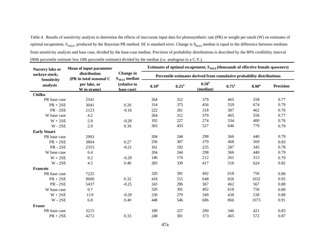
47a

0.10a 0.25a 0.50a

(median)0.75a 0.90a Precision

ChilkoPR base case 2541 264 312 379 465 558 0.77

PR + 2SE 3041 0.20 314 373 456 559 674 0.79PR - 2SE 2123 -0.16 222 261 318 387 462 0.76

W base case 4.2 264 312 379 465 558 0.77W + 2SE 5.9 -0.28 192 227 274 334 400 0.76W - 2SE 2.9 0.39 363 433 527 646 779 0.79

Early StuartPR base case 2993 204 244 298 366 440 0.79

PR + 2SE 3804 0.27 256 307 379 468 569 0.83PR - 2SE 2355 -0.21 161 192 235 287 345 0.78

W base case 6.4 204 244 298 366 440 0.79W + 2SE 9.2 -0.29 146 174 212 261 313 0.79W - 2SE 4.5 0.40 283 339 417 516 624 0.82

FrancoisPR base case 7225 320 391 492 618 756 0.89

PR + 2SE 9600 0.32 418 515 648 826 1032 0.95PR - 2SE 5437 -0.25 243 296 367 462 567 0.88

W base case 9.7 320 391 492 618 756 0.89W + 2SE 13.9 -0.29 230 279 349 438 538 0.88W - 2SE 6.8 0.40 448 546 686 866 1073 0.91

FraserPR base case 3215 189 227 280 346 421 0.83

PR + 2SE 4272 0.33 248 301 373 465 572 0.87

Mean of input parameter distribution

(PR in total seasonal C per lake, orW in grams)

Change in SMAX median

(relative to base case)

Table 4. Results of sensitivity analysis to determine the effects of inaccurate input data for photosynthetic rate (PR) or weight per smolt (W) on estimates of

optimal escapement, SMAX, produced by the Bayesian PR method. SE is standard error. Change is SMAX median is equal to the difference between medians

from sensitivity analysis and base case, divided by the base-case median. Precision of probability distributions is described by the 80% credibility interval

(90th percentile estimate less 10th percentile estimate) divided by the median (i.e. analogous to a C.V.).

Nursery lake or sockeye stock; Sensitivity analysis

Estimates of optimal escapement, SMAX (thousands of effective female spawners)

Percentile estimates derived from cumulative probability distributions

47b

PR - 2SE 2420 -0.25 144 172 211 259 313 0.80W base case 7.4 189 227 280 346 421 0.83

W + 2SE 10.6 -0.28 136 163 200 247 299 0.81W - 2SE 5.2 0.40 264 316 392 486 596 0.85

Late StuartPR base case 10437 661 820 1042 1332 1664 0.96

PR + 2SE 13931 0.34 872 1083 1396 1801 2281 1.01PR - 2SE 7820 -0.25 501 621 780 988 1232 0.94

W base case 6.4 661 820 1042 1332 1664 0.96W + 2SE 9.2 -0.29 475 589 744 948 1179 0.95W - 2SE 4.5 0.40 922 1141 1462 1872 2357 0.98

PittPR base case 606 46 55 67 81 96 0.76

PR + 2SE 906 0.49 69 82 99 121 145 0.77PR - 2SE 405 -0.33 31 37 45 55 64 0.75

W base case 5.8 46 55 67 81 96 0.76W + 2SE 7.4 -0.21 36 43 53 64 76 0.74W - 2SE 4.5 0.27 59 70 85 103 122 0.75

QuesnelPR base case 4995 520 628 780 968 1182 0.85

PR + 2SE 5979 0.19 619 747 931 1168 1432 0.87PR - 2SE 4173 -0.17 439 528 651 809 978 0.83

W base case 4.0 520 628 780 968 1182 0.85W + 2SE 5.7 -0.29 374 450 553 687 839 0.84W - 2SE 2.8 0.39 724 874 1087 1365 1672 0.87

ShuswapPR base case 10148 1454 1800 2286 2923 3668 0.97

PR + 2SE 11957 0.18 1696 2109 2696 3467 4366 0.99PR - 2SE 8612 -0.15 1245 1534 1944 2465 3076 0.94

W base case 2.7 1454 1800 2286 2923 3668 0.97W + 2SE 3.9 -0.29 1050 1288 1631 2076 2595 0.95W - 2SE 1.9 0.40 2018 2491 3211 4126 5206 0.99

a Probability that optimal escapement is less than the value in the body of the table.

0 50 100 km

N

Takla Lake

Trembleur Lake

Stuart Lake

Francois Lake

Fraser Lake

Quesnel Lake

Chilko LakeShuswap

Lake

Pitt Lake

Canada

USA

Figure 1. Fraser River watershed with major sockeye salmon nursery lakes identified.

49

Pro

bab

ility

Photosynthetic rate

Pro

bab

ility

Maximum smolt abundance

Pro

bab

ility

Maximum total smolt biomass / lake

Pro

bab

ility

Smolt weight at high densities

AK lakesBC lakes

Max

imu

m o

bse

rved

sock

eye

smo

lt b

iom

ass

(to

nn

es /

yr)

Photosynthetic rate (tonnes C / yr)

Pro

bab

ility

Smolts (thousands)

Optimal escapementof female spawners

Eff

ecti

ve f

emal

e sp

awn

ers

(th

ou

san

ds)

BC lakes

Step 1

Step 2

Step 3

=

Figure 2. Conceptual diagram of the 3 steps of the Bayesian PR method.

Weight persmolt

Max. totalsmolt biomass

per lake /(( ) )

50

Figure 3. Relationship between maximum observed juvenile sockeye salmon biomass and total

seasonal photosynthetic rate (PR) in log-log space. Data are smolt biomass except for two of the BC

lakes, Shuswap and Quesnel, which are fall fry biomass. Data for Alaskan lakes (solid triangles) are

from Koenings and Burkett (1987) and for BC lakes (solid circles) are from Shortreed et al. (2000).

The dotted line represents the best-fit relationship of the Bayesian PR method, the solid lines illustrate

the extremes of the range of relationships considered by the Bayesian approach, and the dashed line

represents the PR model of Shortreed et al. (2000).

0.01

0.10

1.00

10.00

100.00

1000.00

10000.00

1 10 100 1,000 10,000 100,000

Total seasonal photosynthetic rate (tonnes C * year -1)

Max

imum

obs

erve

d bi

omas

s of

juv

enile

soc

keye

sa

lmon

(to

nnes

* ye

ar-1

)

AK lakes

BC lakes

BabineQuesnel Shuswap

Chilko

51

Figure 4. Estimates of effective female spawners and estimates of smolt abundance at peak smolt

productivity for five BC lakes. The data are from five separate analyses of EFS and smolt data using the

Ricker model to estimate EFS and smolt abundances at the peak of the curve. The dotted line

represents the best-fit relationship of the Bayesian PR method, the solid lines illustrate the extremes of

the range of relationships considered by the Bayesian approach, and the dashed line represents the

smolts per EFS ratio used in the PR model of Shortreed et al. (2000).

0.01

0.10

1.00

10.00

100.00

1,000.00

10,000.00

1 10 100 1,000 10,000 100,000

Peak smolt abundance (thousands)

Effe

ctiv

e fe

mal

e sp

awne

rs (

thou

sand

s)

Babine

Lakelse

Chilko

Cultus

Port John

52

Figure 5. Observed stock and recruit data, maximum likelihood estimates for the Ricker curve,

posterior probability density functions (pdf) for estimates of the escapement to maximize recruits, MAXS ,

from the Bayesian PR method and the S-R analysis or the S-J analysis of 8 Fraser River sockeye

salmon aggregates. Left-hand Y axis refers to observed adult or juvenile abundance; right-hand Y axis

refers to probability for the pdfs of optimal escapement estimated by S-R or S-J analysis (open

triangles) and estimated by the Bayesian PR method (X's).

53a

Effective female spawners (thousands)

Pro

babi

lity

Adu

lt re

crui

ts (

thou

sand

s)Ju

veni

le a

bund

ance

(th

ousa

nds)

Juve

nile

abu

ndan

ce (t

hous

ands

)

Shuswap S-J

0

50,000

100,000

150,000

200,000

0 2000 4000 60000

0.1

0.2

0.3

0.4

Quesnel S-J

0

25,000

50,000

75,000

0 1000 2000 3000 4000 50000

0.1

0.2

0.3

0.4

Chilko S-J

0

10,000

20,000

30,000

40,000

50,000

0 400 800 12000

0.1

0.2

0.3

0.4

Shuswap S-R

0

5,000

10,000

15,000

20,000

0 2000 4000 60000

0.1

0.2

0.3

0.4

Chilko S-R

0

1,000

2,000

3,000

4,000

5,000

0 400 800 12000

0.1

0.2

0.3

0.4

53b

Effective female spawners (thousands)

Pro

babi

lity

Adu

lt re

crui

ts (

thou

sand

s)Francois S-R

0

100

200

300

400

0 25 50 750

0.1

0.2

0.3

0.4

Optimal escapement estimated by the Bayesian

Pitt S-R

0

50

100

150

200

250

0 25 50 75 1000

0.1

0.2

0.3

0.4

Early Stuart S-R

0

400

800

1200

1600

0 200 400 600 8000

0.1

0.2

0.3

0.4Late Stuart S-R

0

2000

4000

6000

0 500 1000 1500 2000 25000

0.1

0.2

0.3

0.4

Fraser S-R

0

500

1000

1500

2000

0 200 400 600 8000

0.1

0.2

0.3

0.4Observed MLE Ricker curve

Pdf of optimal escapement estimated by S-R or S-J analysis

Pdf of optimal escapement estimated by Bayesian PR method

54

Figure 6. Changes in the precision of MAXS estimates from the Bayesian PR method for Pitt Lake

with additional years of photosynthetic rate (PR) and weight per smolt (W) input data.

55Effective female spawners (thousands)

Pro

babi

lity

Pitt Lake

0.00

0.04

0.08

0.12

0.16

20 40 60 80 100

120

140

10 yrs W data

6 yrs W data

2 yrs W data (base case)

1 yr. W data

0.00

0.04

0.08

0.12

0.16

20 40 60 80 100

120

140

10 yrs PR data

6 yrs PR data

2 yrs PR data

1 yr. PR data (base case)

0.00

0.04

0.08

0.12

0.16

0 20 40 60 80 100

120

140

160

10 yrs PR & W data

6 yrs PR & W data

2 yrs PR & W data

1 yr. PR data, 2 yrs W data(base case)

56

Figure 7. Cumulative probability functions comparing three estimates of the escapement to maximize recruits, MAXS , for Pitt Lake sockeye

salmon calculated using the Bayesian PR method and three different input distributions for photosynthetic rate (PR). The mean values of the

input distributions were 606 (base case, solid circles), 906 (base case + 2SE, open squares), and 405 (base case – 2SE, open triangles) metric

tons of carbon. Standard deviation of the input distribution remained at the base-case value.

0.0

0.2

0.4

0.6

0.8

1.0

0 50 100 150 200 250

Effective female spawners (thousands)

Cum

ulat

ive

prob

abili

ty

Base case, PR mean = 606 tonnes C

PR mean = 405 tonnes C

PR mean = 906 tonnes C

Pitt Lake

57

Figure 8. Cumulative probability functions comparing three estimates of the escapement to maximize recruits, MAXS , for Chilko Lake sockeye

salmon calculated using the Bayesian PR method and three different input distributions for smolt weight at high density ( MAXW ). The mean values

of the input distribution were 4.2 (base case, solid circles), 5.9 (base case + 2SE, open squares), and 2.9 (base case – 2SE, open triangles)

0.0

0.2

0.4

0.6

0.8

1.0

0 200 400 600 800 1,000 1,200 1,400

Effective female spawners (thousands)

Cum

ulat

ive

prob

abili

ty

Base case, W mean = 4.2 g

W mean = 2.9 g

W mean = 5.9 g

Chilko Lake

58

grams. Standard deviation of the input distribution remained at the base-case value.

59

Figure 9. Ratio of equilMSY SS , estimated using the Ricker stock-recruitment model, as a function of the Ricker a parameter (recruits per

spawner at low abundance). The solid diamonds represent the Fraser River sockeye aggregates analyzed in this study.

0.25

0.30

0.35

0.40

0.45

0.50

0 5 10 15 20 25

Recruits/spawner at low abundance

SM

SY/S

equi

l

60

Figure 10. Provisional estimates of limit reference points (LRP), as probability density functions

(pdf), determined from two different combinations of estimates of optimal escapement and sockeye

salmon productivity at low abundance for 7 Fraser River sockeye salmon aggregates: 1) PR-based

MAXS and S-R-based Ricker a parameter (stars), 2) S-R-based MAXS and S-R-based Ricker a

parameter (open triangles).

60aEffective female spawners (thousands)

Pro

babi

lity

Francois

0

0.1

0.2

0.3

0.4

0 100 200 300 400

Pitt

0

0.1

0.2

0.3

0.4

0 20 40 60 80

Early Stuart

0

0.05

0.1

0.15

0.2

0.25

0 200 400

Late Stuart

0

0.05

0.1

0.15

0.2

0.25

0 1000 2000

Fraser

0

0.05

0.1

0.15

0.2

0.25

0 200 400

60b

Effective female spawners (thousands)

Pro

babi

lity

Shuswap

0

0.02

0.04

0.06

0.08

0.1

0.12

0.14

0.16

0.18

0 2000 4000

Chilko

0

0.02

0.04

0.06

0.08

0.1

0.12

0.14

0.16

0.18

0 400 800

Pdf of LRP estimated from PR-based SMAX

and S-R-based Ricker a parameter

Pdf of LRP estimated from S-R-based SMAX and S-R-based Ricker a parameter

61

Figure 11. Provisional estimates of limit reference points (LRP), as probability density functions

(pdf), determined from three different combinations of estimates of optimal escapement and

sockeye salmon productivity at low abundance for the Quesnel Lake sockeye salmon aggregate: 1)

PR-based MAXS and S-R-based Ricker a parameter (stars); 2) PR-based MAXS and all plausible

Ricker a values (open circles); and 3) S-J-based MAXS and S-R-based Ricker a parameter (open

triangles).

Effective female spawners (thousands)

Pro

babi

lity

Quesnel

0

0.05

0.1

0.15

0.2

0.25

0.3

0.35

0.4

0.45

0 500 1000 1500 2000 2500 3000

Pdf of LRP estimated from PR-based SMAX

and S-R-based Ricker a parameter

Pdf of LRP estimated from PR-based SMAX

and all plausible Ricker a values

Pdf of LRP estimated from S-J-based SMAX

and S-R-based Ricker a parameter

62

References

Adkison, M.D., and R.M. Peterman. 1996. Results of Bayesian methods depend on details ofimplementation: an example of estimating salmon escapement goals. Fisheries Research. 25:155-170.

Alaska Department of Fish and Game and the Alaska Board of Fisheries. 2000. SustainableSalmon Fisheries Policy for the State of Alaska, March 23, 2000.http://www.state.ak.us/adfg/adfghome.htm (Sept. 2001)

Alaska Department of Fish and Game (ADF&G). 2001. Alaska's conservation mandate.http://www.state.ak.us/adfg/geninfo/hot/brochure.htm (Sept. 2001)

Bradford, M.J. 1995. Comparative review of pacific salmon survival rates. Can. J. Fish. Aquat. Sci.52: 1327-1338.

Bradford, M.J., R.A. Myers, and J.R. Irvine. 2000a. Reference points for coho salmon(Oncorhynchus kisutch) harvest rates and escapement goals based on freshwater production.Can. J. Fish. Aquat. Sci. 57: 677-686.

Bradford, M.J., B.J. Pyper and K.S. Shortreed. 2000b. Biological responses of sockeye salmon tothe fertilization of Chilko Lake, a large lake in the interior of British Columbia. N. A. J. of Fish.Manag. 20: 661-671.

Bugaev, V.F., D.W. Welch, M.M. Selifonov, L.E. Grachev and J.P. Eveson. 2001. Influence of themarine abundance of pink (Oncorhynchus gorbuscha) and sockeye salmon (O. nerka) ongrowth of Ozernaya River sockeye. Fisheries Oceanography 10: 26-32.

Caddy, J.F. and R. McGarvey. 1996. Targets or limits for management of fisheries? N. Am. J.Fish. Manage. 16: 479-487.

de la Mare, W.K. 1998. Tidier fisheries management requires a new MOP (management orientedparadigm). Reviews in Fish Biology and Fisheries. 8: 349-356.

Diewert, R.E. and M.A. Henderson. 1992. The effect of competition and predation on productionof juvenile sockeye salmon (Oncorhynchus nerka) in Pitt Lake. Can. Tech. Rep. Fish. Aquat.Sci. 1853. 51 p.

Eggers, D.M. 2001. ADF&G Escapement goal policy. Presented at the 7th Alaska SalmonWorkshop, "Escapement and the Realities of the New Salmon Management", AnchorageAlaska, Feb. 21-23, 2001.

63

FAO (Food and Agriculture Organization of the United Nations). 1995a. Precautionary approachto fisheries. Part 1: Guidelines on the precautionary approach to capture fisheries and speciesintroductions. Elaborated by the Technical Consultation on the Precautionary Approach toCapture Fisheries (Including Species Introductions). FAO Fisheries Technical Paper No. 350,Part 1. FAO, Rome. 52 p. (Also published in 1996 as FAO Technical Guidelines forResponsible Fisheries No. 2, 54 p.)

FAO (Food and Agriculture Organization of the United Nations). 1995b. The code of conduct forresponsible fisheries. Adopted by the Twenty-eighth session of the FAO Conference inOctober 1995. 41 p. http://www.fao.org/WAICENT/faoinfo/fishery/FIconde.htm (Sept. 2001)

Fisheries and Oceans Canada. 1998. A new direction for Canada's Pacific Salmon Fisheries, policypaper, released for review October 1998.http://www-comm.pac.dfo-mpo.gc.ca/english/newdirections/default.htm (Sept. 2001)

Fisheries and Oceans Canada. 2000. Wild Salmon Policy, discussion paper released for reviewMarch 2000. http://www-comm.pac.dfo-mpo.gc.ca/english/newdirections/default.htm (Sept.2001)

Foerster, R.E. 1954. On the relation of adult sockeye salmon (Oncorhynchus nerka) returns toknown smolt seaward migrations. J. Fish. Res. Bd. Canada 11(4): 339-350.

Foerster, R.E. 1968. The Sockeye Salmon, Oncorhynchus nerka. Fisheries Research Board ofCanada. Ottawa.

Gabriel, W.L. and P.M. Mace. 1999. A review of biological reference points in the context of theprecautionary approach. In: Restrepo, V.R. (ed). Proceedings of the Fifth National StockAssessment Workshop. Providing scientific advice to implement the precautionary approachunder the Magnuson-Stevens Fishery Conservation and Management Act. U.S. Department ofCommerce, National Marine Fisheries Service, NOAA Technical Memorandum NMFS-F/SPO-40.

Garcia, S.M. 2000. The precautionary approach to fisheries management: progress review andmain issues: 1995-2000. In: Nordquist, M.H. and J.N. Moore (eds). Current Fisheries Issuesand the Food and Agriculture Organization of the United Nations, publ. by Kluwer LawInternational, Netherlands.

Geiger, H.J., and J.P. Koenings. 1991. Escapement goals for sockeye salmon with informative priorprobabilities based on habitat considerations. Fisheries Research. 11: 239-256.

Gelman, A., J.B. Carlin, H.S. Stern, and D.B. Rubin. 1995. Bayesian Data Analysis. Chapman andHall. London.

64

Henderson, M.A., R.E. Diewert, J. Hume, K. Shortreed, D. Levy, and K. Morton. 1991. Thecarrying capacity of Pitt Lake for juvenile sockeye salmon (Oncorhynchus nerka). Can. Tech.Rep. Fish. Aquat. Sci. 1797. 161 p.

Hilborn, R. 1985. Simplified calculation of optimum spawning stock size from Ricker's stockrecruitment curve. Can. J. Fish. Aquat. Sci. 42: 1833-1834.

Hilborn, R. and C.J. Walters. 1992. Quantitative Fisheries Stock Assessment: Choice, Dynamicsand Uncertainty. Chapman and Hall. New York.

Hill, R.A. and B.J. Pyper. 1998. Implications of a Bayesian approach for simulating salmonpopulation dynamics. In: Fishery stock assessment models. Alaska Sea Grant CollegeProgram. AK-SG-98-01: 873-887.

Hume, J.M.B., K.S. Shortreed, and K.F. Morton. 1996. Juvenile sockeye rearing capacity of threelakes in the Fraser River system. Can. J. Fish. Aquat. Sci. 53: 719-733.

Johnston, N.T., E.A. Parkinson, A.F. Tautz and, B.R. Ward. 2000. Biological reference points forthe conservation and management of steelhead, Oncorhynchus mykiss. Canadian StockAssessment Secretariat Research Document 2000/126. Available at the web site:http://www.dfo-mpo.gc.ca/csas/ (Sept. 2001)

Koenings, J.P., and R.D. Burkett. 1987. Population characteristics of sockeye salmon(Oncorhynchus nerka) smolts relative to temperature regimes, euphotic volume, fry density andforage base within Alaskan lakes. In: H.D. Smith, L. Margolis, and C. C. Wood (eds).Sockeye salmon (Oncorhynchus nerka) population biology and future management. Can.Spec. Publ. Fish. Aquat. Sci. 96.

Koenings, J.P., and G.B. Kyle. 1997. Consequences to juvenile sockeye salmon and thezooplankton community resulting from intense predation. Alaska Fishery Research Bulletin.4(2): 120-135.

Korman, J., R.M. Peterman, and C.J. Walters. 1995. Empirical and theoretical analyses ofcorrection of time-series bias in stock-recruitment relationships of sockeye salmon. Can. J. Fish.Aquat. Sci. 52: 2174-2189.

Kyle, G.B., J.P. Koenings, and B.M. Barrett. 1988. Density-dependent, trophic level responses toan introduced run of sockeye salmon (Oncorhynchus nerka) at Frazer Lake, Kodiak Island,Alaska. Can. J. Fish. Aquat. Sci. 45: 856-867.

Myers, R.A., A.A. Rosenberg, P.M. Mace, N. Barrowman, and V.R. Restrepo. 1994. In searchof thresholds for recruitment overfishing. ICES J. Mar. Sci. 51: 191-205.

65

Oregon Department of Fish and Wildlife (ODFW). 1992. Oregon's Wild Fish Management Policy.http://www.dfw.state.or.us/ODFWhtml/InfoCntrFish/PDFs/BKGWildFish.pdf (Sept. 2001)

Pacific Salmon Commission (PSC). 1998. Thirteenth annual report 1997/98. Available from PSC,600 – 1155 Robson Street, Vancouver, BC, V6E 1B5.

Peterman, R.M. 1981. Form of random variation in salmon smolt-to-adult relations and its influenceon production estimates. Can. J. Fish. Aquat. Sci. 38: 1113-1119.

Peterman, R.M. 1982. Nonlinear relation between smolts and adults in Babine Lake sockeyesalmon (Oncorhynchus nerka) and implications for other salmon populations. Can. J. Fish.Aquat. Sci. 39: 904-913.

Peterman, R.M. 1984. Density-dependent growth in early ocean life of sockeye salmon(Oncorhynchus nerka). Can. J. Fish. Aquat. Sci. 41: 1825-1829.

Punt, A.E. and R. Hilborn. 1997. Fisheries stock assessment and decision analysis: the Bayesianapproach. Reviews in Fish Biology and Fisheries 7: 35-63.

Quinn II, T.J. and D.M. Eggers. 2001. Applying Alaska groundfish management strategy to Alaskasalmon escapement goals. Presented by T. Quinn at the 7th Alaska Salmon Workshop,"Escapement and the Realities of the New Salmon Management", Anchorage Alaska, Feb. 21-23, 2001.

Quinn II, T.J., R. Fagen, and J. Zheng. 1990. Threshold management policies for exploitedpopulations. Can. J. Fish. Aquat. Sci. 47: 2016-2029.

Ricker, W.E. 1997. Cycles of abundance among Fraser River sockeye salmon (Oncorhynchusnerka). Can. J. Fish. Aquat. Sci. 54: 950-968.

SAS Institute Inc. 1988. SAS Procedures guide, release 6.03. SAS Institute Inc., Cary, N.C.

Schmidt, D.C., S.R. Carlson, and G.B. Kyle. 1998. Influence of carcass-derived nutrients onsockeye salmon productivity of Karluk Lake, Alaska: importance in the assessment of anescapement goal. N. Am. J. Fish. Manage. 18: 743-763.

Shortreed, K.S., J.M.B. Hume, and K.F. Morton. 1996. Trophic status and rearing capacity ofFrancois and Fraser lakes. Can. Tech. Rep. Fish. Aquat. Sci. 993.

Shortreed, K.S., J.M.B. Hume, and J.G. Stockner. 2000. Using photosynthetic rates to estimatethe juvenile sockeye salmon rearing capacity of British Columbia lakes. In: E.E. Knudsen, C.R.Steward, D.D. MacDonald, J.E. Williams, and D.W. Reiser (eds). Sustainable fisheriesmanagement: Pacific salmon. CRC Press LLC.

66

Shortreed, K.S., K.F. Morton, K. Malange, and J.M.B. Hume. 2001. Factors limiting juvenilesockeye production and enhancement potential for selected B.C. nursery lakes. CanadianStock Assessment Secretariat Research Document 2001/098. Available at the web site:http://www.dfo-mpo.gc.ca/csas/ (Dec. 2001)

Stobbard, A.R. and D.R. Harding. 1996. Pitt River Sockeye Hatchery Update – 1995. Can.Manuscr. Rep. Fish. Aquat. Sci. 2353: 38p.

Taylor, G.C. and M.J. Bradford. 1993. Results of rotary auger trap sampling, lower Stuart River,British Columbia, in April and May 1992. Can. Manuscr. Rep. Fish. Aquat. Sci. 2211: 18 p.

United Nations. 1995. Agreement for the implementation of the provisions of the United NationsConvention on the Law of the Sea of 10 December 1982 relating to the conservation andmanagement of straddling fish stocks and highly migratory fish stocks. A/CONF. 164/37 (8September 1995).

Walters, C., and D. Ludwig. 1994. Calculation of Bayes posterior probability distributions for keypopulation parameters. Can. J. Fish. Aquat. Sci. 51: 713-722.

Washington Department of Fish and Wildlife (WDFW). 1997. Policy of Washington Department ofFish and Wildlife and Western Washington Treaty Tribes Concerning Wild Salmonids.http://www.wa.gov:80/wdfw/faq/wspfaq.htm (Sept. 2001)

West, C.J. and J.C. Mason. 1987. Evaluation of sockeye salmon (Oncorhynchus nerka)production from the Babine Lake Development Project. In: H. D. Smith, L. Margolis, andC. C. Wood (eds). Sockeye salmon (Oncorhynchus nerka) population biology and futuremanagement. Can. Spec. Publ. Fish. Aquat. Sci. 96.

Wood, C.C., D.T. Rutherford, D. Bailey, and M. Jakubowski. 1998. Assessment of Sockeyesalmon production in Babine Lake, British Columbia with forecast for 1998. Can. Tech. Rep.Fish. Aquat. Sci. 2241.

67

Appendix A:

A Bayesian approach to parameter estimation for linear relationships

A Bayesian approach was used to take uncertainty into account when quantifying the

parameters for all of the linear relationships fit in this study (i.e. to quantify parameters for

relationships used in steps 1 and 3 of the Bayesian PR method and all the S-R and S-J analyses).

Bayesian methods combine prior information with likelihoods based on available data to compute

posterior probability distributions for the estimates of interest. In this way degrees of belief are

quantified for all probable values of the estimates, given the data. Given the linear relationship:

(A1) εββ ++= XY 10

where Y is the dependent variable, 0β is the intercept, 1β is the slope, X is the independent

variable, and ε is the stochastic error term assumed to be normally distributed with standard

deviation σ , each plausible set of 0β and 1β parameters defines a different relationship between

the X and Y variables. In this study, for each of the linear relationships, plausible ranges for the slope

and intercept parameters were considered while σ was treated as known. θ denotes the

parameter vector ( 0β , 1β , σ̂ ), where σ̂ is the MLE for σ . For a given parameter combination

iθ , the posterior probability of iθ given the observed data, D, was determined using Bayes

theorem (Gelman et al. 1995):

(A2)∑

=

jjj

iii

PDL

PDLDP

)()(

)()()(

θθ

θθθ

68

where )( iDL θ is the likelihood of the data given iθ , )( iP θ is the prior probability assigned to iθ ,

and ∑j

jj PDL )()( θθ is the sum of the products of the likelihoods times priors for all parameter

combinations considered.

For both 0β and 1β , plausible ranges of the prior probability distribution were divided into

a number of discrete bins and an equal probability (i.e. a uniform prior) was assigned to each bin.

For a given iθ , the likelihood of the data across all data points t was computed using the normal

likelihood function:

(A3)

−= ∏ 2

2

2exp

2

1)(

i

t

t ii

wDL

σπσθ

where )( 10 ttt XYwii

ββ +−= and ∏t

is the product of all t terms to the right. The prior

probabilities and likelihoods of the various parameters combinations ( iθ ) were then combined using

Bayes' theorem (Equation A2) to generate the posterior distribution for θ , also called the joint

posterior probability distribution for the slope and intercept parameters.

69

Appendix B:

Photosynthetic rate and weight per smolt data for Fraser River sockeye

salmon

Photosynthetic rate (PR) data used in this study were from 9 BC sockeye salmon nursery

lakes (K.S. Shortreed, personal communication). Shortreed et al. (2000) described the collection of

PR data in detail. Values of seasonal average daily PR (mg C m-2d-1) for each lake were converted

to total seasonal PR (tonnes C per lake) ( TOTALPR ) by multiplying by lake surface area and length of

the growing season, assumed to be 180 days (May 1 to October 31); Shortreed et al. (2000).

Where available, multiple years of annual estimates of PR were averaged to obtain mean total

seasonal PR for each lake (Table 2).

Weight per smolt ( MAXW ) data for Fraser River sockeye salmon are sparse for most stocks

(Table 2). Since MAXW at high smolt density was not always available, where possible I used MAXW

data for cohorts whose parents were not low in abundance relative to the range in historical records

(i.e. relatively high; also, spawner abundance was used as an index of smolt density). Annual

estimates of MAXW were converted from grams to tonnes and lake-specific mean values were

calculated in cases where more than one annual estimate was available.

Lake-specific normally distributed loge estimates of both PR and MAXW were used in the

application of the Bayesian PR method. Standard errors for these distributions were based on the

amount of lake-specific data and estimates of interannual variability in PR and MAXW . Exploratory

data analysis revealed that within-lake annual variability in loge estimates of both PR and MAXW was

70

approximately normally distributed. Interannual variability ( 2log totale PRσ and 2

log MAXe SWσ ) was estimated

using variance components analysis (SAS VARCOMP procedure, SAS Institute Inc. 1988) on all

multiple annual observations available. For PR, data were from 8 of the 9 study lakes because only

one annual estimate of PR was available for Pitt Lake. Data used in the MAXW variance components

analysis included 34 years from Babine Lake (Wood et al. 1998), 28 pre-fertilization years from

Chilko Lake (J.M.B. Hume, personal communication), and 7 years from Cultus Lake (Foerster

1954). These MAXW data represent only those cohorts in relatively high abundance that had been

presumably subject to density-dependent growth. The variance components analysis procedure

assumed equal interannual variability among lakes and these data do not contradict that assumption

(i.e. variance does not increase as a function of PR or MAXW ).

For application of steps 1 and 2 of the Bayesian PR method, loge TOTALPR and loge MAXSW

for each lake were described by normal distributions:

(B1)

nPRPR TOTALe PR

TOTALeTOTALe

2log,logN~log

σ

(B2)

nSWSW MAXe SW

MAXeMAXe

2log,logN~log

σ

where n in each case is the number of annual estimates of either PR or MAXW available for that lake

(Table 2).

71

Appendix C:

Photosynthetic rate (PR) for Early and Late Stuart sockeye salmon

stocks

Quantifying the normal distribution to describe TOTALPR for the rearing habitats of the Early

and Late Stuart sockeye salmon stocks required additional analysis because the rearing habitats for

their juveniles overlap in Trembleur Lake. There are no abundance estimates for juvenile sockeye

salmon rearing in the Stuart Lakes, so I apportioned the nursery habitat of Trembleur Lake between

the two stocks by making various assumptions and using stock-specific estimates of escapement.

Assuming that juveniles rear in the lake directly downstream of their natal stream means that

juveniles of the Early Stuart stock have exclusive use of nursery habitat in Takla Lake and use some

portion of Trembleur Lake habitat, whereas juveniles of the Late Stuart stock have exclusive use of

Stuart Lake and also use some portion of Trembleur Lake. Using escapement estimates

apportioned to each natal stream (J.M.B. Hume, personal communication), for only the dominant

cycle line where fry density was high relative to other years, I calculated the relative proportion of

spawners, from each of the two stocks, that used streams flowing into Trembleur Lake. On

average, 26% of the spawners using these streams in years of high abundance are from the Early

Stuart stock, and 74% are from the Late Stuart stock. Assuming equal egg deposition and equal

egg-to-fry survival rates between stocks, and assuming all fry consume equally, the estimated index

of lake productivity (total seasonal PR) for Trembleur Lake was apportioned to each stock based

on the relative abundances of the spawners. The loge TOTALPR representing the nursery habitat for

each stock is a function of the loge TOTALPR for the two lakes contributing to each stock's habitat:

72

(C1) =)(log tEarlyStuarPRTOTALe

( ))(26.0)(log kTrembleurLPRTaklaLkPR TOTALTOTALe •+

(C2) =)(log LateStuartPRTOTALe

( ))(74.0)(log kTrembleurLPRStuartLkPR TOTALTOTALe •+

The average variance (var) in loge TOTALPR for each of the habitat areas is also a function of the

variance calculated for each contributing lake:

(C3) )(26.0)()( 2 kTrembleurLvarTaklaLkvartEarlyStuarvar •+=

(C4) )(74.0)()( 2 kTrembleurLvarStuartLkvarLateStuartvar •+=

Variance for each contributing lake was computed from standard deviations in loge TOTALPR

(Appendix B, Equation B1).