Page 1

Pre-print version of paper published as: Preene, M (2019). Design and interpretation of packer permeability tests for geotechnical purposes. Quarterly Journal Of Engineering Geology, 52, 2, May, 182–200.

DESIGN AND INTERPRETATION OF PACKER PERMEABILITY TESTS FOR GEOTECHNICAL

PURPOSES Author Martin Preene* Abbreviated title: Packer permeability tests for geotechnical purposes This revision 10 October 2018.

Page 2

DESIGN AND INTERPRETATION OF PACKER PERMEABILITY TESTS FOR GEOTECHNICAL PURPOSES

Abstract Packer permeability tests are used routinely in geotechnical investigations to allow estimation of hydraulic conductivity by analysis of pressure/flow rate response during controlled injection of water into a section of borehole, isolated by packers. This paper is a review of the hydraulic fundamentals of the packer permeability test methods and analyses used routinely in geotechnical investigations and discusses the usefulness and limitations of the test. Guidance is given on design of tests, including the maximum hydraulic conductivity that can be measured by the method. Interpretation of tests must recognise that responses are influenced by the entire test system – the host rock, the borehole and any associated zone of disturbance, water quality (injected water and water in the host rock), the packers or isolation system and the head/flow rate measurement system. It is proposed that, for geotechnical projects, presenting test results as a Q-H diagram (plotting injection flow rate vs. applied excess head) is useful and allows results to be classified against seven conventional and three unconventional test responses (which expand on earlier work by Houlsby (1976) and others). Guidance is given on the selection of values of hydraulic conductivity, for geotechnical design purposes, from various types of test responses. Packer permeability tests are a routine part of ground investigations for construction and tunnelling projects in rock. The method, described in BS EN ISO 22282-3:2012 (and previously in BS5930:2010 and earlier editions of the same standard), is used to estimate hydraulic conductivity in rock. The test, based on methods originally developed for grouting projects, involves analysis of pressure/flow rate response during controlled injection of water into a section of borehole, isolated by packers. Typical test sequences produce multiple values of hydraulic conductivity, complicating the selection of values for geotechnical design. The packer permeability test in context The packer permeability test can be considered a microcosm of routine geotechnical field testing; it has several limitations, in relation to hydraulic conditions during the test, and the methods of analysis commonly used. In an ideal world these tests would be replaced by other test types and analysed differently, to give better estimates of hydraulic conductivity. However, in practice, packer permeability tests are an established part of the geotechnical industry, and were in the historic British Standards and are in the current European Standards. They will continue to be carried out and geotechnical analysts and designers will continue to be presented with data from these tests, and will face the challenge of using the data for geotechnical purposes. This paper is intended to aid geotechnical practitioners in the planning and interpretation of packer permeability tests, as carried out routinely for geotechnical projects. The origins and

Page 3

hydraulic fundamentals of the packer permeability test are reviewed, and the usefulness and limitations of the tests are discussed. Recommendations are given for test design and interpretation where tests are used to provide data for geotechnical designs. The essentials of the packer permeability test The focus of this paper is on routine packer permeability tests used for geotechnical investigations. These tests are commonly called packer tests or Lugeon tests (as will be discussed later, the latter term is used inaccurately for most geotechnical applications). In this context, the principal objective of the tests is to estimate hydraulic conductivity, a term equivalent to coefficient of permeability (often referred to as permeability in geotechnical documents) as used in geotechnical design, to provide parameters for design in rock where groundwater flow is a key consideration (for example contaminant transport, seepage below retaining walls, slope stability, tunnel seepage, construction dewatering). It is widely accepted that these tests have significant limitations, both in execution and analysis, but the tests are in the current Eurocode 7 suite of standards (BS EN 1997-1:2004; BS EN ISO 22282-3:2012) and are likely to remain a staple of ground investigations. More complex in-situ hydraulic tests and analysis are used on some hydrogeological studies for water resources, nuclear repository studies and deep mining projects (Banks, 1992; Gringarten, 2008), but are not covered here. A packer permeability test is typically carried out in a borehole in rock, where unlined sections of the borehole are stable enough to stand unsupported. A section of the borehole is isolated by inflatable packers to form a ‘test section’ and flow of water is induced into or out of the test section, with the flow rate and pressure head in the test section monitored. By setting test sections at different depths in the borehole, multiple tests may be carried out sequentially along the borehole length after drilling is completed, or can be executed incrementally, during pauses in drilling, as the borehole is deepened. A double packer test (Fig. 1a) has a test section isolated above and below by packers. In a single packer test (Fig. 1b) the test section is between a packer and the base of the borehole. In principle, a packer permeability test can be carried out by either injecting water into the test section (inflow or pumping-in tests), or removing water from the test section (outflow or pumping-out tests). Several studies, including Brassington & Walthall (1985) and Price & Williams (1993) indicate that pumping out tests tend to give more representative values of hydraulic conductivity. However, in relatively small diameter boreholes it is much easier to inject water than to remove it (which may require a down hole pump and more sophisticated equipment). In routine geotechnical investigations injection tests are used almost exclusively, and are the focus of the current paper. Practical limitations of the packer permeability test It is important to recognise the imperfections of the packer test method as a means to determine hydraulic conductivity for geotechnical purposes. The primary limitation is that the test is ‘small-scale’ in that it is of short duration (the total injection time of a typical test is 50 to 75 minutes) and can only influence a modest volume of rock around the borehole.

Page 4

To illustrate the scale of the host rock that is tested, consider a geotechnical packer test in a rock of mean hydraulic conductivity 1 x 10-6 m/s. Such a test might inject water at a maximum rate of approximately 10 l/min/metre of borehole for 75 minutes. If, for the sake of simplicity, it is assumed that the injected water moves outward radially on a cylindrical front then the injected water (0.53 m3 per metre of borehole in in this case, estimated from equation A6 in Appendix 3) will occupy a cylinder of modest radius, controlled in part by the effective porosity of the rock. In a Triassic sandstone where the porosity might be 0.25 (Shand et al., 2002), the diameter of the theoretical cylinder of injected water would be around 1 m. The hydraulic effect of the injection will extend further as the host groundwater is displaced outward radially by the injected water, but significant changes in hydraulic head will be limited (in this case) to within a few metres of the borehole. This a very simplified example; in a real packer test water will tend to flow along pathways controlled by bedding and other discontinuities, and the hydraulic effect of the injected water may propagate much further from the borehole. However, modelling by Bliss & Rushton (1984) indicated that packer tests only disturb groundwater flow for a distance of about 10 m from the borehole. When visualising the zone of rock that is significantly affected by a packer test, a radius of 10 m from the borehole is reasonable maximum distance. In rock of lower hydraulic conductivity the affected radius may be much smaller. Therefore, the hydraulic conductivity values from packer tests will be biased toward the conditions close to that test section (including any disturbance effects around the borehole). A packer test can be contrasted with a well pumping test (Kruseman & De Ridder, 1992; Preene & Roberts, 1994; Misstear et al., 2017), where a well is pumped continuously for an extended period (1 to 7 days pumping being typical of geotechnical practice). Such longer-term pumping tests can change groundwater heads at much greater distances from the test borehole, and can provide ‘larger scale’ mass hydraulic conductivity values more representative of conditions away from the test borehole. Other limitations of packer tests include:

• The hydraulic properties derived from the test relate to water being injected into rock. These properties may be different to those for geotechnical projects where water flows out of rock (e.g. tunnel seepage, construction dewatering).

• The test provides data on injection rates and pressure responses for a test section of finite length. The test response is therefore controlled by both the properties of the rock (hydraulic conductivity K) and the geometry of the test section (including the length L of the test section). The analyses discussed in this paper actually calculate transmissivity T. The transmissivity of the test section is the product of the hydraulic conductivity and test length (T = Kaverage.L). Kaverage is calculated as Kaverage = (T/L) and is an average hydraulic conductivity for the test section. It may not be straightforward (without reference to the geological model and other data, such as borehole geophysics) to determine whether outflow is via a single fracture, multiple fractures, or more general percolation through the rock mass.

• The overall test response may be influenced by the equipment issues, including leakage of water past packers intended to isolate the test section.

• The application of high injection flow rates or high excess heads may affect the rock properties by erosion, plugging or jacking of fractures. Hydraulic conductivity values from such tests may not be representative of geotechnical problems where lower heads apply – e.g. contaminant migration or seepage below retaining walls.

Page 5

• Because water is injected into the test section, water quality can affect hydraulic conditions during the test. A particular problem occurs if the water used for injection is even slightly dirty or turbid – the suspended fine-grained particulate matter in the water can clog or plug fractures and intergranular flow paths on the walls of the test section. A lesser problem is geochemical clogging where the injected water may react with the host water or rock. To avoid this problem, ideally the injected water should be groundwater from the same stratum as the test section. However, in most geotechnical investigations this is not practicable and the water is typically sourced from local utilities. Any potential geochemical clogging is likely to be a second order effect compared to clogging caused by the use of ‘dirty’ water.

Development of current packer testing practice UK practice in packer permeability tests has evolved gradually. The essence of the modern packer test derives from the work of Lugeon (1933), as described later in this paper. However, perhaps the first modern analysis of the packer permeability tests for geotechnical investigations in the UK is Muir Wood and Caste (1970) for tests in chalk for the 1964–65 Channel Tunnel Study Group investigations. That paper outlines the use of flow rate vs. excess head plots to interpret different types of hydraulic behaviour during a test; these methods are still used in test assessment today, and are analogous to the recommendations in the current paper. In the 1970s a series of papers in the Quarterly Journal of Engineering Geology collectively set the template for modern practice and analysis including the five step pressure increment method commonly used (Lancaster Jones, 1975; Houlsby, 1976, Pearson and Money, 1977). These papers appear to be the basis of the packer testing sections in the original UK Code of Practice for Site Investigations (BS5930:1981), and are still routinely referenced in industry reports. In the following decades, papers by Bliss and Rushton (1984), Brassington and Walthall (1985) and Walthall (1990) applied more rigorous hydrogeological approaches to test analyses. Ewert (1994), Quiñones-Rozo (2010) and Hartwell (2015) re-visited the fundamentals of these tests and highlighted some limitations and common misunderstandings. The Lugeon test The origins of the packer permeability test probably lie in drill stem testing for oil industry wells in the early 20th century (testing reservoir properties in sections of boreholes isolated by packers is still a staple of the modern oil industry). However, it is generally accepted that modern geotechnical test methods can be traced back to the work of Maurice Lugeon (Lugeon, 1933) who defined a standard test protocol (the Lugeon test) and a new unit, the Lugeon coefficient (Lu), to characterise the hydraulic behaviour of fractured rock around a test borehole, as an aid to the grouting programmes for dam foundations being constructed around that time. It is sometimes forgotten that the Lugeon test was not developed to determine hydraulic conductivity as a geotechnical designer might understand today. The test essentially assesses ‘water take’ to determine how much water can be injected into a small diameter

Page 6

borehole, as a predictor of grout injection rates (background on Lugeon tests for grouting design is given by Paisley et al., 2017). Lugeon’s innovation was to set standardised test parameters, giving an empirical measure of water take (the Lugeon coefficient) calculated on a common basis for each test. This allowed a rational comparison of water take between boreholes and between tests at different levels in the same borehole. The Lugeon coefficient Lu is defined as water absorption measured in litre/minute per metre of test section at an excess pressure of 10 bar (1000 kPa; 1 MPa; 102 m head of water); excess pressure is defined as the pressure above the ambient groundwater pressure at the midpoint of the test section 𝐿𝑢 = !!"""

" (1)

where Q1000 is the water take of the borehole (in litre/min) at an excess pressure of 1000 kPa, and L is the length of the test section. Equation 1 requires the use of the stated units to obtain the correct values; equivalent equations for Imperial Units are used in North American practice. It is interesting to note that borehole diameter does not feature in this equation, which emphasises the empirical nature of Lu values. BS5930:2010 states that Lugeon did not specify the diameter of the borehole, which is usually assumed to be approximately 76 mm (equivalent to an NQ size cored hole). Published literature typically uses a correlation between the Lugeon coefficient and hydraulic conductivity of 1 Lu » 1 x 10-7 m/s (Appendix 1 shows an example correlation of Lu and hydraulic conductivity units). The Lugeon test in its original form presumes that relatively high excess pressures will be used (ideally 1000 kPa), based on its origin as a test to mimic the injection of grout into fractured rock. In many civil engineering applications, the use of such high excess pressures is neither necessary to obtain useful results, nor advisable (due to the risk of fracture dilation or hydrojacking). If an excess pressure of 1000 kPa is not applied, a test is not strictly a Lugeon test, and a Lu value cannot be determined. In these cases, a modified Lugeon coefficient (Lumod) can be calculated from equation 2, using the assumption that inflow is proportional to excess pressure 𝐿𝑢#$% =

!#"× &'''

($ (2)

where QP is the water take of the borehole (in litre/min) at an excess pressure Pt (kPa); again, this equation requires the use of the stated units to obtain the correct values. In practice, in the geotechnical industry, quoted Lu values typically take test pressures into account and are therefore Lumod. This is illustrated by equation 3, which is reproduced from Houlsby (1976), which is directly equivalent to equation 2 𝐿𝑢𝑔𝑒𝑜𝑛𝑐𝑜𝑒𝑓𝑓.= 𝑤𝑎𝑡𝑒𝑟𝑡𝑎𝑘𝑒(𝑙𝑖𝑡𝑟𝑒𝑠/min 𝑝𝑒𝑟𝑚) × &'*+,

-./01,.//2,.(*+,/) (3)

Page 7

In the remainder of this paper, it will be assumed that the derivation of Lu values takes test pressures into account, and so Lu and Lumod will be used interchangeably. The packer permeability test The parameters of a true Lugeon test are strictly defined and may not be appropriate in many geotechnical applications. Furthermore, such tests are designed to produce Lu values, rather than the hydraulic conductivity values required for geotechnical design under Eurocode 7 (BS EN 1997-1:2004) and similar standards. While there are correlations between Lu and hydraulic conductivity in m/s (Appendix 1), the most appropriate approach and terminology for geotechnical projects is to consider the tests as packer permeability tests (not Lugeon tests) and to have the primary derived parameters as hydraulic conductivity in m/s (not Lugeon coefficient). During planning and interpretation, the test should be viewed as a generic hydraulic borehole test, albeit one where the geometry is constrained by packers, rather than being a specialised type of test. Analytical equations to derive hydraulic conductivity are discussed below; notation is given in Appendix 2. Focussing on the hydraulic fundamentals can aid critical assessment of results. The starting point for any hydraulic test is Darcy’s law 𝑄 = 𝐾𝑖𝐴 (4) where Q is the injection flow rate to the test section, K is the hydraulic conductivity, A is the area of flow and i is the hydraulic gradient (the hydraulic gradient is created by the application of an excess head H). Darcy’s law is predicated on laminar flow (termed Darcian flow) where, for a given geometry (for example a borehole test section), Q and H have a linearly proportional relationship. It is generally accepted that packer permeability tests in rock where flow is predominantly via fine fracture networks are dominated by Darcian flow, and a plot of Q vs. H will be approximately linear. However, where more open fractures are present, allowing higher flow rates, non-Darcian (turbulent) flow will occur, and the flow rate will increase under-proportionally with excess head, as energy is lost to turbulence. A Q vs. H plot will be non-linear for at least part of the test. For tests in boreholes, Darcy’s law is often represented by Hvorslev’s formula (Hvorslev, 1951), arranged to calculate values of hydraulic conductivity from observations of flow rate into and out of a borehole under the effect of an excess head H (measured relative to original groundwater level). H can be related to the excess pressure Pt in the test section by H = Pt/gw, where gw is the unit weight of water 𝐾 = !

56 (5)

F is a shape factor, a function of the geometry of the test zone, representing A and the flow path element of i. Hvorslev’s equation assumes saturated conditions (i.e. the test section is entirely below groundwater level), laminar flow conditions, and that the water injected or

Page 8

removed during the test does not change background groundwater level around the test. A further implicit assumption is that the borehole is 100% hydraulically efficient – i.e. the borehole itself does not introduce any hydraulic resistance above that from the properties of the rock mass. The analysis methods for routine packer permeability tests are usually based on the assumption that each phase of the test acts as an individual steady state constant head injection test, with an applied excess head of H and an injection flow rate of Q. A further assumption that flow out of the test section is Darcian (laminar). Hvorslev’s formula (equation 5) can be applied, and various shape factors F can be used (based on length of the test section, borehole diameter and consideration of the geometry of the water flow around the test section) to calculate hydraulic conductivity. Derivation of hydraulic conductivity values The derivation of hydraulic conductivity values from the results of packer tests conventionally uses shape factors based on the work of Hvorslev (1951) to account for the geometry (length L and diameter D) of the test section. With the exception of equations 11 and 12, the hydraulic conductivity values from the equations below are average values for the test section; the test section may comprise a mixture of zones of higher and lower hydraulic conductivity, for example due to differences in bedding and fracturing. Unlike the empirical formulae (equations 1 to 3) used to derive the Lugeon coefficient which are specific to certain combinations of units, the equations below can be used with any combination of SI units. However, to obtain hydraulic conductivity values in m/s, normal practice is to use L, D and H in metres and Q in m3/s (not in litre/min, which is the unit commonly recorded in the field). For a test in a vertical borehole of diameter D in a uniform isotropic aquifer, the generic Hvorslev (1951) shape factor for a test section of length L results in:

𝐾 = !786"

𝑙𝑛 @"9+ B1 + 𝐿

7

𝐷7E F'.;G (6)

For L/D greater than 4 this becomes 𝐾 = !

786"𝑙𝑛 B7"

9F (7)

In practice, most packer tests will have L/D > 4, and equation 7 is widely used for routine analysis (this is the equation used in BS5930:2010 and the earlier versions of that standard). The same equation is used for double packer tests and single packer tests (where there is potentially some ‘end effect’ outflow directly from the base of the test section). For L/D > 4 the flow from the end effect is a very small proportion of the total flow and does not have a major effect on calculated hydraulic conductivity. In anisotropic hydraulic conductivity conditions, where the vertical hydraulic conductivity is Kv, and the horizontal hydraulic conductivity is Kh, then equation 7 for L/D >4 becomes

Page 9

𝐾< =!

786"𝑙𝑛 B7#"

9F (8)

where

𝑚 = B𝐾< 𝐾=E F'.;

(9) An alternative formulation is where it is assumed that the aquifer is very highly anisotropic (Kh>>Kv) and flow from the test section is entirely horizontal within the length L of the test section. This gives an equation equivalent to the Thiem equation for radial steady state flow to/from a well 𝐾< =

!786"

𝑙𝑛 B7>%9F (10)

where Ro is the radius of influence of the change in groundwater levels caused by the test. This is the equation presented in Annex C of BS EN ISO 22282-3:2012. Packer tests typically do not include monitoring of surrounding boreholes, so Ro cannot be measured and must be estimated or assumed. However, due to the log term, the calculated hydraulic conductivity is not especially sensitive to Ro; BS EN ISO 22282-3:2012 indicates that Ro is typically between 10 m and 100 m. In practice, Ro values of 25 to 30 m are commonly applied. A key problem with assessing the hydraulic conductivity from a packer test section of length L is that the equations presented here effectively calculate the average hydraulic conductivity Kaverage, assuming the injected water leaves the test section uniformly across the cylindrical boundary. In many cases this is not the case: for example, where more permeable sandstone beds are present within a mudstone sequence in Coal Measures strata. If the strata descriptions indicate there are two to three orders of magnitude difference in hydraulic conductivity between zones of high and low hydraulic conductivity strata, then the water take of the low hydraulic conductivity stratum can be ignored, and the approximate equivalent hydraulic conductivity K¢ of the permeable zones can be estimated as: 𝐾? = 𝐾+=.,+@. × B

""&F (11)

where L¢ is the assessed total thickness of the permeable stratum within the test section. Equation 11 is appropriate for discrete permeable zones within the test section, where individual zones are of thickness more than 0.1 to 0.5 m. However, if core descriptions or borehole geophysics indicate that flow is likely to be concentrated in one or more discrete fractures, solutions based the equation of Barker (1981) can be used. As applied in Bliss and Rushton (1984), this assumes that the entire injection flow rate leaves the test section (of diameter D) via single horizontal fracture of aperture width b and fracture hydraulic conductivity Kf and then passes, from the fracture into the wider aquifer mass of anisotropic hydraulic conductivity Kh, Kv (which can be estimated from packer tests that do not intercept major fractures). If the fracture aperture width b is known from borehole CCTV or televiewer images then the equivalent hydraulic conductivity kf of the fracture can be

Page 10

estimated for each Q/H data point using equation 12. Kf appears twice in the equation, so this should be solved iteratively by substituting in estimates of Kf until the Q/H value is achieved !6= 78A'*

BCD(')

*+,("./001)"./34(5(6E (12)

Analysis methods for packer tests intercepting discrete transmissive fractures are discussed in Price (1994).

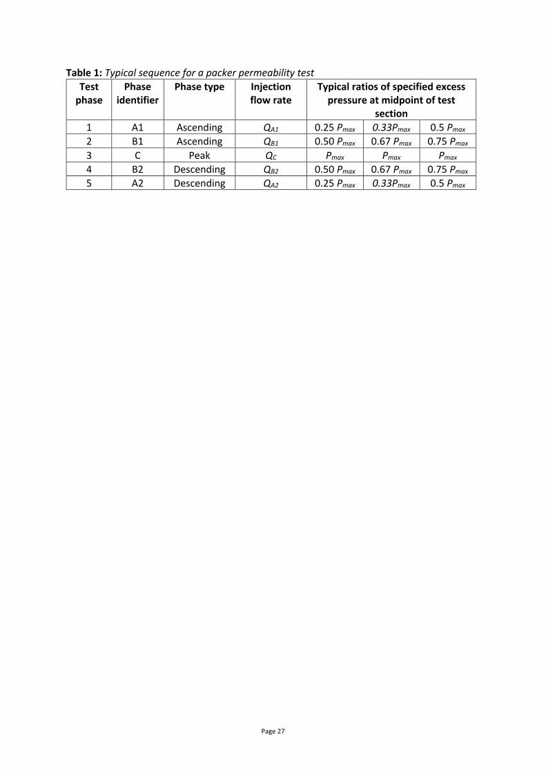
Test design To obtain the most useful and representative geotechnical information, the test parameters for a programme of packer permeability tests should be designed. This includes determining the depth and length of test sections, and setting target excess pressures. A check should also be made that the available equipment can achieve the estimated flow rate/water volume requirements, based on the anticipated rock hydraulic conductivity. It is important that the injected water is clean and free from suspended solids; this reduces the risk of clogging or plugging of the test section. Further guidance on planning and execution of packer permeability tests is given in Appendix 3. The test methods used in geotechnical practice are defined in BS EN ISO 22282-3: 2012, where the tests are described as ‘Water pressure tests in rock’. The requirements of the standard do not constrain either the number and sequence of test injection phases, nor the duration of each phase. In UK geotechnical practice, packer permeability tests most commonly comprise five consecutive injection phases (each phase of the same duration – typically 10 or 15 minutes, longer durations are sometimes used). Injection pressures are varied rapidly at the end of each phase, giving a step-wise transition of pressure between phases. The de-facto standard approach is to use three ascending and descending test pressures, A, B, C in sequence A1-B1-C-B2-A2. Effective results can be obtained with various ratios of excess head in the A, B, C phases, as shown in Table 1. Each phase is effectively a constant head water injection test. The benefit of multiple injection phases at different pressures is that the relationship between injection flow rate and excess head can be graphed as a Q-H plot, which can provide insight into the hydraulic response during the test. Upper hydraulic conductivity limit of equipment Packer tests derive hydraulic conductivity values from the relationship between excess head H and injection flow rate Q. For a given set of test equipment of maximum injection flow rate Qmax, and for a given target excess head, there is a maximum hydraulic conductivity Kmax that can be determined. If zones of high hydraulic conductivity may be encountered, a check should be made at test design stage by applying Qmax and the target Hmax into the relevant hydraulic conductivity equations in this paper. Calculations in Appendix 3 show that for equipment with Qmax of 150 l/min (a common equipment configuration) a packer test with a target excess head of 25 m is not capable of

Page 11

determining a hydraulic conductivity of more than around 5 x 10-5 m/s. If higher hydraulic conductivities are anticipated (and assuming the injection pumping equipment cannot be uprated), the test could be designed with lower target excess pressures. However, even with a target excess head of 10 m, a 150 l/min injection test can only determine hydraulic conductivity up to around 1 x 10-4 m/s. This is interesting, because (as noted by Hartwell (2015)), the British Standard guidance BS EN ISO 22282-1:2012, in its Table 2 ‘Recommended applicability for different test procedures’ indicates that packer permeability tests can be used to determine hydraulic conductivity up to 10-2 m/s. In practice, the range of application of packer tests in BS EN ISO 22282-1:2012 is not achievable at the high hydraulic conductivity end; values higher than around 10-4 m/s cannot be measured with standard equipment. Furthermore, careful test design of injection flow rates and excess heads (including assessment of pipework friction losses) are required to determine hydraulic conductivity between 10-5 and 10-4 m/s. Test length Test length L and depth Z of the midpoint of the test must be specified based on the conceptual geological and hydrogeological model used in the ground investigation design. Test programmes can either: test the whole borehole length, section by section, to obtain a vertical profile of hydraulic conductivity vs. depth: or, target testing at specific horizons inferred to be more or less permeable than the typical host rock. There is no single template for packer testing programmes, but examples include:

i. Early phases of ground investigation, where generic data is sought on the distribution of hydraulic conductivity with depth, may use a series of packer tests with consecutive test sections from groundwater level down to the base of the borehole. Test lengths of between 3 m and 10 m are typical.

ii. In later ground investigation phases, if there is an expectation of variation in hydraulic conductivity with depth (e.g. as might occur due to weathering in the Sherwood Sandstone Group or the Chalk Group), tests with consecutive test sections may be carried out over the relevant depths, from groundwater level downward. Test lengths of between 2 m and 6 m are typical.

iii. Where the bedrock geology is believed to be affected by faults or zones or multiple discontinuities that may be more permeable, tests should be carried out at the depth of the permeable zone and, for comparison purposes, at other depths. The length of test section may be controlled by the need to locate the packers at suitable levels to seal against relatively intact rock.

iv. If discrete permeable horizons are expected (e.g. Tea Green Marls within the Mercia Mudstone Group, or hardgrounds within the Chalk Group) then test sections can be targeted to these zones. Test lengths of between 1 m and 3 m are typical. The same approach can be used if potential permeable features are identified from core logs or borehole geophysics. For comparison, some tests should be done at other depths where the features are not indicated to be present.

A common problem is that the packers may not provide an effective seal against the borehole wall; this is not always apparent at the time of the test, and can affect test results. If there is any information (e.g. from drilling records, core logs or borehole geophysics) that borehole diameter is uneven at certain depths (for example due to flint horizons in Chalk),

Page 12

the field team should be prepared to vary the test depths to avoid setting packers at those levels. For geotechnical investigations, it is relatively unusual to attempt packer permeability tests in the unsaturated zone above the groundwater level. The assumptions of the Hvorslev method described in this paper are invalid in unsaturated conditions and the hydraulic response of a test in this zone will be different to tests in the saturated zone, due to the injected water filling voids and changing rock saturation. It is also difficult to assess the initial groundwater head, and therefore the applied excess head (the test section would be reported as ‘dry’ before the start of the test). Test injection pressure The maximum test excess pressure Pmax should be selected with care. Pmax is sometimes based on the pressure that can be applied without risk of dilating or displacing existing fractures/joints (known as hydrojacking) in the rock around or above the test section. A commonly quoted criterion (in Houlsby (1976) and elsewhere) is that Pmax should not exceed 1 pound per square inch (psi) per foot of depth, subject to a 150 psi (approximately 100 m head) limit. Updated to SI units this is approximately 22.5 kPa per m depth. The studies of Bjerrum et al. (1972) indicate that a Pmax of 22.5 kPa per m depth does have some risk of hydraulic dilation of fractures/joints. Furthermore, as discussed below, there is often no need for high excess pressures to obtain representative hydraulic conductivity values. Bjerrum et al. (1972) recommend that, in rock subject to isotropic stress conditions, the maximum excess test pressure Pmax should not exceed the vertical effective stress s¢v; this is also consistent with the recommendations of Walthall (1990) 𝑃#+F < 𝜎=? (13) This is significantly lower than 22.5 kPa per m depth. In a simple set of ground conditions, where rock is present from the surface, with an initial groundwater level Hw and a hydrostatic pore water pressure distribution, at depths below groundwater level (i.e. Z > Hw) s¢v can be approximately estimated from 𝑃#+F < 𝛾,$GH . 𝑍 − 𝛾I . (𝑍 − 𝐻J) (14) where grock is the unit weight of the rock and gw is the unit weight of water (routinely taken as 10 KN/m3 in geotechnical calculations). An example calculation of maximum test pressures is given in Table 2 (Hmax is the maximum excess head in the test section, where Hmax = Pmax/gw). The test pressures estimated from equations 13 and 14 are maxima, to reduce the risk of hydraulic dilation of fractures/joints, and should not automatically be used. Testing at significantly lower excess pressures can still give good results, with less risk of high pressures opening up fractures or flow pathways and giving unrepresentatively high hydraulic conductivity values. In practice, tests with applied excess heads in the range 5 to

Page 13

25 m (50 kPa < Pt < 250 kPa) are appropriate for many geotechnical investigations. Where any of the target pressures have an equivalent water head in the test section that is below the level of the water injection system (typically around 1 m above ground level), the pressure measurement system must be the down hole pressure sensor type (Fig. A2a), rather than the surface mounted pressure gauge type (Fig.A2b). Presentation of test results Tests should be analysed, where results are used to obtain numerical values of hydraulic conductivity. However, analysis should be guided by interpretation, where results are critically assessed and related to the wider geological model. This requires a basic understanding of typical relationships between applied excess head H and injection flow rate Q. Analysis and interpretation of tests can be aided by graphing injection flow rate Q vs. applied excess head H (Q-H plots). This approach was proposed by Pearson and Money (1977) and is directly analogous to flow rate vs. injection pressure diagrams (P-Q plots) used by various authors, including Muir-Wood and Caste (1970) and Ewert (1994). Q-H plots are preferable over P-Q plots because water heads in metres are easier to visualise than pressure in kPa when assessing the driving impetus (head or pressure) during test interpretation. A Q-H plot is shown schematically in Fig. 2; it is essential that the origin (0,0) is included. The Darcian hydraulic conductivity of any (Q, H) point is proportional to the gradient of a line joining the point to the origin. Visualised in this way, it is easy to interpret hydraulic conductivity changes in test plots such as those shown in Fig. 3, by considering that tests where later phases plot with a steeper gradient to the origin imply that hydraulic conductivity is increasing during the test. Conversely, if later phases plot with a shallower gradient to the origin, this implies a decrease in hydraulic conductivity is indicated from phase to phase. It is important to note that the test response is not solely derived from the rock being tested, but relates to the test system – the host rock, the borehole and any associated zone of disturbance, the packers or isolation system and the head/flow rate measurement system. For example, if a test shows an apparent increase in hydraulic conductivity between phases (i.e. greater Q/H values) this could be due to the opening/erosion of rock fractures (changes in hydraulic conditions in the rock), or could be due to leakage past packers (changes in equipment performance). Categories of packer test responses Comparison of test responses with ‘standard’ patterns can aid interpretation, and an approach commonly used in UK practice is to compare test responses with five categories proposed by Houlsby (1976). The current paper proposes an improved approach, which classifies Q-H plots against seven ‘conventional’ responses (which include Houlsby’s five cases) and a further three ‘non-conventional’ responses. It is also proposed that the categories be described strictly in terms of test response, rather than jumping directly to interpretation of the hydraulic behaviour of the rock, as might implied by titles of Houlsby’s categories.

Page 14

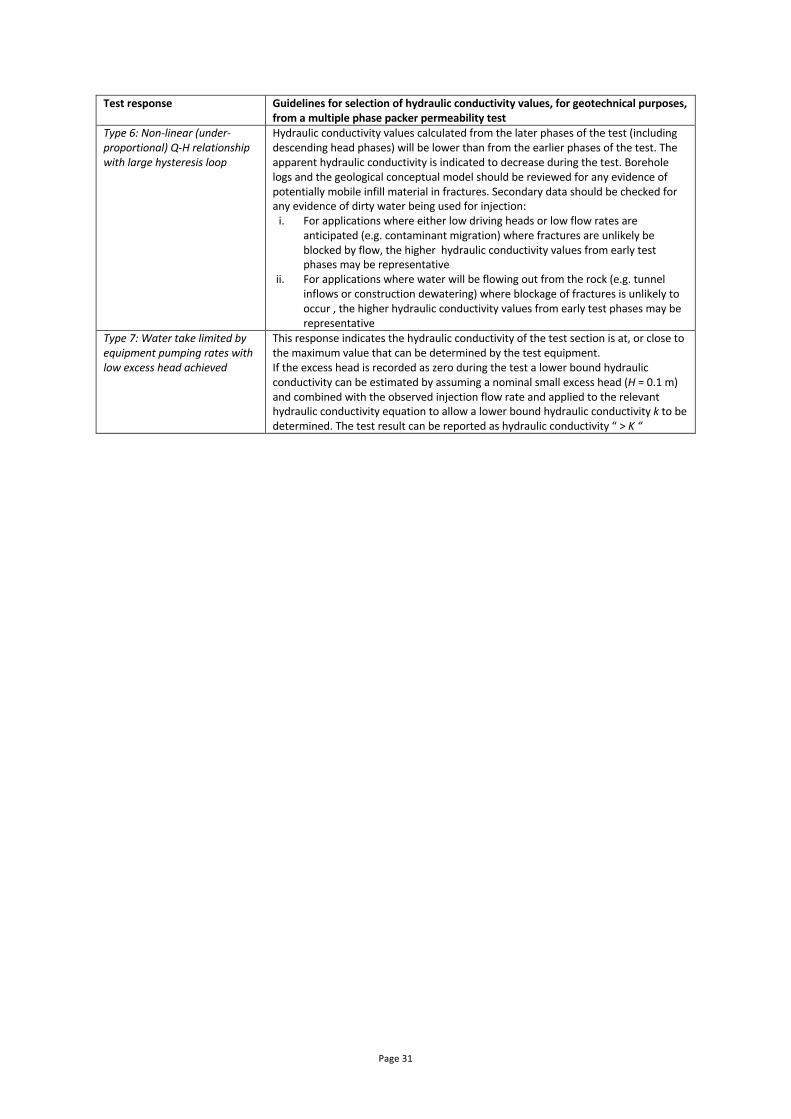
Figs. 3 and 4 show Q-H plots for the conventional and non-conventional test responses, respectively, for test phases of the A1-B1-C-B2-A2 pattern. Each data point represents the Q and H for each phase, and the points are linked in sequence by straight lines. The plot must also include origin (Q=0, H=0) at both the start and of the test, when the applied excess head is zero. The seven conventional test responses types (Fig. 3) are: Type 1: Zero water take Categorised by effectively zero water injection rate at all excess heads (this is an additional case to those of Houlsby). This response has only one plausible interpretation – a test carried out in rock of very low hydraulic conductivity, with good packer seals achieved. Type 2: Linear Q-H relationship with small hysteresis loop Injection flow rate and excess head have an approximate linear relationship (including the line to the origin), with only a small hysteresis between the ascending and descending test phases. Hydraulic conductivity is essentially independent of excess head (this is Houlsby’s laminar case). A possible interpretation is Darcian flow out from the test section. Type 3: Non-linear (under-proportional) Q-H relationship with small hysteresis loop Injection flow rates are not linearly related to excess head, and the apparent hydraulic conductivity reduces as excess head increases, with only a small hysteresis between the ascending and descending test phases, so hydraulic conductivity is not permanently reduced during the test (this is Houlsby’s turbulent case). A possible interpretation is turbulent (non-Darcian) flow causing greater head losses as the water flows out from the borehole, resulting in lower apparent hydraulic conductivity. Type 4: Non-linear (over-proportional) Q-H relationship with small hysteresis loop Injection flow rates are not linearly related to excess head, and the apparent hydraulic conductivity increases as excess head increases, with only a small hysteresis between the ascending and descending test phases, so hydraulic conductivity is not permanently increased during the test (this is Houlsby’s dilation case). Possible interpretations include: existing bedding planes or other discontinuities in the rock are opened up by the applied pressure and close when pressure is removed; and/or packer leakage or movement that causes the test section to lose water at higher heads, but closes with reduced excess head. Type 5: Non-linear (over-proportional) Q-H relationship with large hysteresis loop Apparent hydraulic conductivity increases for each phase, including descending heads, this gives a significant hysteresis loop, where hydraulic conductivity is greater in the descending A2, B2 phases compared to the ascending A1, B1 phases (this is Houlsby’s wash out case). Possible interpretations include: an increase in hydraulic conductivity of the rock caused by the test, due to movement/erosion of infill in fractures in such a way that they do not block flow paths, or permanent rock movements caused by the testing; and/or leakage past the packers that disturbs or erodes the rock, so that leakage paths do not close with reduced excess head. Type 6: Non-linear (under-proportional) Q-H relationship with large hysteresis loop

Page 15

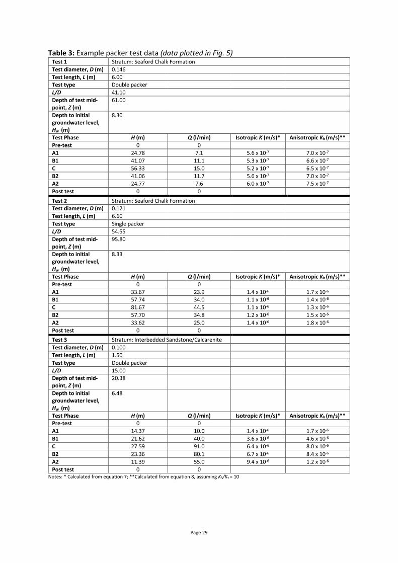
Apparent hydraulic conductivity decreases for each phase, including descending heads, this gives a significant hysteresis loop, where hydraulic conductivity is lower in the descending A2, B2 phases compared to the ascending A1, B1 phases (this is Houlsby’s void filling case). Possible interpretations include: a decrease in hydraulic conductivity of the rock caused by the test, with possible mechanisms including a) water filling and pressurising of voids or discontinuities not linked to a wider network, b) movement or swelling of infill in fractures in such a way that they become trapped and block flow paths, c) clogging of rock fractures due to use of dirty water for injection. Type 7: Water take limited by equipment pumping rates with low excess head achieved This response is categorised by the injection rate quickly reaching close to the maximum injection flow rate Qmax for the test equipment, which is not able to establish an excess head in the test section (this is an additional case to those of Houlsby). Possible interpretations include: the test section intersects highly permeable fractures or discontinuities; and/or excessive water leakage past the packers; and/or poor selection of test equipment with an under-rated injection pump. The three non-conventional test responses (Fig. 4) are: Type 8: Sudden excess head drop to zero The injection flow rate shows a conventional Q-H relationship up to a given head, at which point the flow rate increases rapidly and the excess head drops to almost zero. Possible interpretations include: packer failure or a major fracture opening suddenly as the applied excess head clears a blockage. Type 9: Flow rate initiates at significant non-zero excess head The injection flow rate is effectively zero at lower excess heads, and increases suddenly under the higher heads of later phases. Possible interpretations include: hydrojacking or fracture dilation in a ‘tight’ rock of very low hydraulic conductivity; and/or clearing of a blockage in a sediment filled fracture; and/or packer leakage or movement; and/or the rest water level assumed in analysis is higher than assumed (by an amount greater than the excess head in phases A1/A2). Type 10: Excess head does not build until significant non-zero flow rate The excess head is effectively zero at lower injection rates, and increases suddenly under the higher flow rates of later phases. A possible interpretation is that the rest water level assumed in analysis is lower than assumed (by an amount greater than the excess head in phases A1/A2). Example test plots The value of a Q-H diagram in visualising the test behaviour can be illustrated by plotting data from three contrasting tests. Table 3 presents summary data for two tests in the same borehole in the Seaford Chalk Formation in the confined aquifer of the London Basin in the UK and one test in sandstone and calcarenite in the United Arab Emirates. In all the tests L/D >> 4, and the hydraulic conductivity was calculated using equation 7 for assumed isotropic conditions and equations 8 and 9 for an assumed anisotropy of Kh/Kv = 10.

Page 16

These tests are plotted as Q vs. H in Fig. 5. Although the calculations of hydraulic conductivity use m3/s, it is convenient to plot Q in l/min. Theses plots show: Test 1: The plot in Fig. 5 shows an approximately linear Q-H relationship consistent with Type 2 response (comparable with Fig. 3(b)). As shown conceptually in Fig. 2, the hydraulic conductivity of any (Q, H) point is proportional to the slope of a line joining the point to the origin. The interpretation of Test 1 is that the calculated hydraulic conductivity hardly varies between test phases, and the lack of a hysteresis loop indicates that the hydraulic properties of the rock immediately around the test section have hardly been affected by the test. Test 2: The plot in Fig .5 shows a non-linear (under proportional) Q-H relationship consistent with Type 3 response (comparable with Fig. 3(c)). This indicates that the calculated hydraulic conductivity varies between test phases. The slope from the origin to the data points to the C phase is less steep than the slope to the B1 and B2 phases, which in turn has a shallower slope than the A1 and A2 phases. This indicates that the calculated hydraulic conductivity reduces when higher heads are applied. However, the lack of a significant hysteresis loop indicates that the hydraulic properties of the rock have hardly been affected by the test. This is consistent with turbulent (non-Darcian) flow causing proportionally greater head losses at higher injection rates. It is interesting to note that without the origin (0,0) point the A, B and C phases form an approximately linear sequence, and misinterpretation as a Type 2 response is possible. This highlights the importance of including the origin as part of the data plot. It is interesting to compare Test 1 and Test 2, carried out at different depths in the same stratum in the same borehole. Test 2 shows significantly greater injection rates and calculated hydraulic conductivity than Test 1 and is the deeper test, with the test midpoint approximately 68 m below the top of the Chalk. Taken alone, these packer tests are slightly surprising, because conceptual models for hydraulic conductivity of the Chalk in the confined London basin typically assume that the depths below the top of the Chalk at which significant water-bearing fractures occur are in the order of a few tens of metres, generally no more than 50 m (Streetly et al., 2018). In the absence of other data, the expectation would be that the deeper test would have lower injection rates and lower calculated hydraulic conductivity. However, in this case description of rock core and televiewer borehole geophysics both indicated that steely dipping fractures intercepted the borehole below approximately 90 m and were absent at shallower depths. This supported the interpretation of the Test 2 response as potentially resulting from turbulent flow from discrete fractures. Test 3: The plot in Fig. 5 shows a non-linear (over proportional) Q-H relationship with a significant hysteresis loop consistent with Type 5 response (comparable with Fig. 3(e)). The slope from the origin to the data points increases for A1, B1, C, B2, A2, which indicates that the calculated hydraulic conductivity increases for each phase. A key aspect is that a significant hysteresis loop indicates that the hydraulic properties of the rock have changed during the test – hydraulic conductivity has permanently increased around the test section. The rock being tested was an interbedded sandstone and calcarenite, where the geological model predicted sand-filled fracture zones within rock mass. The test response is consistent

Page 17

with the injected water washing away or eroding fracture infill, and locally increasing hydraulic conductivity. The test pump had a nominal maximum capacity of 90 l/min, and the data indicates that the maximum excess head achieved was limited by the capacity of the pump. Derivation of hydraulic conductivity values A packer test of the A1-B1-C-B2-A2 pattern has five data points for Q and H. For a given geometry of the test section, equations 6 to 12 can be used to estimate a Darcian hydraulic conductivity for each point. In essence, the method treats each phase of the test as a steady-state constant head injection test, with each phase independent of the other; five values of hydraulic conductivity are obtained for each test of this type. Each hydraulic conductivity value is associated with the relevant excess head, and there may be a significant range of values from a single test. Potential errors in test results Like other forms of in-situ hydraulic conductivity tests, there are multiple potential errors in packer test results, including:

a. Application of methods of analysis in conditions when the basic assumptions of the method are not valid – examples include tests in the unsaturated zone above groundwater level, or where the hydraulic conductivity of the test section is dominated by a small number of very permeable fractures.

b. Errors in the design or analysis of the test – examples include assuming an incorrect initial groundwater level when analysing the test results.

c. Problems with the test execution – examples include leakage past or around packers, restrictions in pumps or pipework system limiting applied heads or flow rates or causing fluctuations during test phases (when steady state conditions should apply), and use of dirty or sediment-laden water for injection.

d. Errors in measurement of field observations – examples include mis-readings of flowmeters or pressure gauges, and out of calibration equipment (flowmeters and pressure sensors).

e. Errors in processing of field observations to produce input data for hydraulic conductivity calculations – examples include mis-calculation of the excess head in the test section.

f. Errors in calculation of hydraulic conductivity values for each test phase – examples include arithmetical errors or using inappropriate units (such as using flow rates in litre/min when attempting to calculate hydraulic conductivity in m/s).

Understanding potential errors can be very useful when reviewing test results, especially in cases where the test responses could permit more than one interpretation. Interpretation of packer test results A geotechnical designer must assess the ‘characteristic value’ of parameters, potentially including hydraulic conductivity. Eurocode 7 (BS EN 1997-1:2004) states ‘the characteristic value of a geotechnical parameter shall be selected as a cautious estimate of the value affecting the occurrence of the limit state’. Where packer tests are part of the hydraulic conductivity dataset, in order to select representative values, designers should understand the typical forms of test results to inform parameter selection.

Page 18

One of the challenges of using packer test data is that each test produces multiple values of hydraulic conductivity (five in the case of an A1-B1-C-B2-A2 test), and for some test responses it is clear the test has modified the hydraulic conductivity around the borehole. The most ‘representative’ hydraulic conductivity values should be selected based on the type of test response. Houlsby (1976) proposed a protocol, still used widely, for selecting suitable hydraulic conductivity values from a packer test, based on the type of overall test response. However, Houlsby’s method is rather prescriptive and was primarily intended for grouting projects. Based on experience of multiple projects where packer permeability tests were applied in geotechnical designs, the current paper proposes different guidelines for selection of hydraulic conductivity values from packer tests (Table 4). Use of the hydraulic conductivity values requires consideration of the following:

i. How will the estimated value be used in the geotechnical design? For design cases combining hydraulic conductivity with either natural or low imposed hydraulic gradients (e.g. contamination migration, or slope seepages) it may be appropriate to use hydraulic conductivity derived from test phases at lower heads and flow rates. Conversely, where higher hydraulic gradients are expected (e.g. tunnel inflows or construction dewatering ) it may be appropriate to use hydraulic conductivity from test phases at higher heads and flow rates. As described elsewhere in the current paper, hydraulic conductivity values from routine packer tests give small-scale values of hydraulic conductivity, and are obtained by injecting water into the rock. Packer tests can be a useful data source when developing characteristic values for construction dewatering and tunnel projects, but where hydraulic conductivity will have a major impact on a project, well pumping tests (Kruseman & De Ridder, 1992; Preene & Roberts, 1994; Misstear et al., 2017) should be considered to obtain values of large-scale hydraulic conductivity.

ii. Are the test results calculated and presented appropriately? Relevant checks include: has the excess head in the test section been calculated correctly from the field data; are the data represented correctly on a Q-H plot? For example, is the origin point included to allow linear responses to be identified?

iii. The test response should be critically reviewed in the context of the geological and hydrogeological model. Examples include: where (turbulent) non-Darcian flow is indicated (Type 3), or if very high water takes are reported (Type 7), are very permeable fractures or fractured zones expected?; or, for Types 6 and 7, where the hydraulic conductivity of the rock around the borehole is indicated to change, is there evidence of infill in fractures that could be eroded or moved to open or block flow paths?

iv. For types of test responses where the test characteristics could be due to either the rock behaviour or other test factors (such as packer leakage or clogging due to use of dirty water) the available secondary data (Table A2) should be reviewed to help identify possible factors influencing test behaviour.

Conclusion Packer tests are used routinely in geotechnical investigations to allow hydraulic conductivity to be assessed from analysis of controlled injection of water into a section of borehole,

Page 19

isolated by packers. It is important that the designers and analysts of the tests understand the hydraulic fundamentals of the test, including the limitations of the method. In particular, for a given maximum injection rate, there is an upper limit to the hydraulic conductivity that can be determined; for high capacity pumps (up to 150 l/min) the maximum hydraulic conductivity (averaged over the test section) that can be determined is around 1 x 10-4 m/s. It is also noted that the relatively high applied excess heads (up to 100 kPa) associated with Lugeon tests are not needed to obtain useful hydraulic conductivity values for geotechnical purposes. In practice, applied excess heads in the range 5 to 25 m are appropriate for many geotechnical investigations. It is proposed that, for geotechnical projects, presenting test results as a Q-H diagram (plotting injection flow rate vs. applied excess head, including the origin point (0,0)) is useful and allows results to be classified against seven conventional and three unconventional test responses (which expand on earlier work by Houlsby (1976) and others). Interpretation of tests must recognise that responses are influenced by the entire test system – the host rock, the borehole and any associated zone of disturbance, water quality (injected water and water in the host rock), the packers or isolation system and the head/flow rate measurement system. Guidance is given on the selection of values of hydraulic conductivity, for geotechnical design purposes, from various types of test responses. References Banks, D. 1992. Estimation of apparent transmissivity from capacity-testing of boreholes in bedrock aquifers. Applied Hydrogeology, 4/92, 5–19. Barker, J.A. 1981. A formula for estimating fissure transmissivities from steady state injection-test data. Journal of Hydrology, 52, 337–346. Bjerrum, L., Nash, J.K.T.L., Kennard, R.M. & Gibson, R.E. 1972. Hydraulic Fracturing in field permeability testing. Géotechnique, 22, 319–332. Bliss, J. & Rushton, K. 1984. The reliability of packer tests for estimating the hydraulic conductivity of aquifers. Quarterly Journal of Engineering Geology, 17, 81–91. Brassington, F.C & Walthall, S. 1985. Field techniques using borehole packers in hydrogeological investigations. Quarterly Journal of Engineering Geology, 18, 181–193. BS 5930: 1981. Code of Practice for Site Investigation. British Standards Institution, London. BS 5930: 1999 amended 2010. Code of Practice for Site Investigation. British Standards Institution, London. BS EN 1997-1: 2004. Eurocode 7: Geotechnical Design – Part 1: General Rules. British Standards Institution, London. BS EN ISO 22282-1 :2012. Geotechnical Investigation and Testing – Geohydraulic Testing, Part 1: General Rules. British Standards Institution, London.

Page 20

BS EN ISO 22282-3 :2012. Geotechnical Investigation and Testing – Geohydraulic Testing, Part 3: Water Pressure Tests in Rock. British Standards Institution, London. Ewert, F. 1994. Evaluation and interpretation of water pressure tests. Grouting in the Ground. Thomas Telford, London. 20, 141–162. Gringarten, A.C. 2008. From straight lines to deconvolution: the evolution of the state of the art in well test analyses. SPE Reservoir Evaluation and Engineering, 11, 1, SPE-102079-PA, Society of Petroleum Engineers, London, 41–62. Hartwell, D.J. 2015. Permeability testing problems in rock. Proceedings of the XVI ECSMFGE, Geotechnical Engineering for Infrastructure and Development. ICE Publishing, London, 2846–2852. Houlsby, A.C. 1976. Routine interpretation of the Lugeon water-test. Quarterly Journal of Engineering Geology, 9, 303–313. Hvorslev, M J. 1951. Time Lag and Soil Permeability in Groundwater Observations. Waterways Experimental Station, Corps of Engineers, Bulletin No.36, Vicksburg, Mississippi. Kruseman, G.P. & De Ridder, N.A. 1990. Analysis and Evaluation of Pumping Test Data. International Institute for Land Reclamation and Improvement, Publication 47 (2nd edition), Wageningen, The Netherlands. Lancaster-Jones, P.F.F. 1975. Technical note: The interpretation of the Lugeon water-test. Quarterly Journal of Engineering Geology, 8, 151–154. Lugeon, M. 1933. Barrages et Geologie. Dunod, Paris. Misstear, B.D.R, Banks, D. & Clark, L. 2017. Water Wells and Boreholes, 2nd edition. Wiley, Chichester. Muir Wood, A.M. & Caste G. 1970. In-situ testing for the Channel Tunnel. In-situ Investigation in Soils and Rocks. British Geotechnical Society, London, 79–85. Paisley, A.C., Wullenwaber, J. & Bruce, D.A. 2017. Practical aspects of water pressure testing for rock grouting. 5th International Grouting, Deep Mixing, and Diaphragm Walls Conference. International Conference Organization for Grouting (ICOG), Honolulu, Oahu, Hawaii. Pearson, R. & Money, M.S. 1977. Improvements in the Lugeon or packer permeability test. Quarterly Journal of Engineering Geology, 10, 221–240. Preene, M. & Roberts, T.O.L. 1994. The application of pumping tests to the design of construction dewatering systems. Groundwater Problems in Urban Areas (Wilkinson, W B, ed.). Thomas Telford, London, 121–133.

Page 21

Price, M. 1994. A method for assessing the extent of fissuring in double porosity aquifers, using data from packer tests. Future Groundwater Resources at Risk, Proceedings of the Helsinki Conference, 13–16 June 1994. International Association of Hydrological Sciences (IAHS) Publication No. 222, 271–278. Price, M. & Williams, A.T. 1993. A pumped double-packer system for use in aquifer evaluation and groundwater sampling. Proceedings of the Institution of Civil Engineers, Water, Maritime and Energy, 101, April, 85–92. Quiñones-Rozo, C. 2010. Lugeon test interpretation, revisited. Collaborative Management of Integrated Watersheds, US Society of Dams, 30th Annual Conference, 405–414. Shand, P. Tyler-Whittle, R. Morton, M. Simpson, E. Lawrence, A R. Pacey, J. & Hargreaves, R. 2002. Baseline Report Series 1: The Permo-Triassic Sandstones of the Vale of York. British Geological Survey Commissioned Report No. CR/02/102N. Streetly, M.J. Daily, P.D. Farren, E.R, Hoad, N. & Jones, M.A. 2018. Developments in the conceptual understanding of groundwater flow in the Chalk in London. Engineering in Chalk: Proceedings of the Chalk 2018 Conference (Lawrence, J.A. Preene, M. Lawrence, U.L. & Buckley, R. (Eds)). ICE Publishing, London, 645–650. Walthall, S. 1990. Packer testing in geotechnical engineering. Field Testing in Engineering Geology (Bell, F.G. Culshaw, M.G. Cripps, J.C. and Coffey, J.R. (Eds)). Geological Society Engineering Geology Special Publication No. 6, London, 345–350.

Page 22

Appendix 1 Correlation between Lugeon coefficient and hydraulic conductivity The equations in the main text allow a relationship to be developed between Lugeon coefficient Lu and hydraulic conductivity K. Table A1 shows hydraulic conductivity calculated from equation 7 for a 76 mm diameter borehole at the standard Lugeon test parameters of 1 l/min per metre of borehole at an excess head H of 1000 kPa. The equivalent hydraulic conductivity of 1 Lu varies with L/D and for this example is between 0.9 x 10-7 and 1.5 x 10-7 m/s, as plotted in Fig. A1. This is the basis of typical published correlations of 1 Lu » 1 x 10-7 m/s.

Page 23

Appendix 2 Notation A : Area of flow b: Fracture aperture width Chw : Hazen-Williams roughness coefficient D: Borehole diameter d: Internal diameter of pipework F : Hvorslev’s shape factor H: Excess head (above ambient groundwater level) at midpoint of test section Hf : Frictional head loss in packer testing pipework Hg : Height of the pressure gauge above ground level Hmax: Maximum excess head in the test section Hw : Depth to initial groundwater level i : Hydraulic gradient K : Hydraulic conductivity (coefficient of permeability) Kaverage : Average hydraulic conductivity over the test section Kf : Equivalent hydraulic conductivity of fracture Kv : Vertical hydraulic conductivity Kh : Horizontal hydraulic conductivity Kmax : Maximum hydraulic conductivity that can be determined with injection rate of Qmax K’: Equivalent hydraulic conductivity of discrete permeable zones within test section L: Length of the test section L’: Assessed total thickness of discrete permeable zones within test section Lu : Lugeon coefficient Lumod : modified Lugeon coefficient m : Hydraulic conductivity transformation ratio lp : Effective length of pipework Pg : Gauge pressure in above ground injection pipework Pt : Excess water pressure (above ambient groundwater level) at the mid-point of the test section Pmax : Maximum excess water pressure (above ambient groundwater level) at the mid-point of the test section Q : Injection flow rate to the test section Q1000 : Water take of borehole (in litre/min) at an excess pressure of 1000 kPa during a Lugeon test Qmax : Maximum injection flow rate possible with a given set of equipment QP : Water take of the borehole (in litre/min) at an excess pressure P (kPa) during a modified Lugeon test Qx: Injection flow rate during phase x of test (phases A1-B1-C-A2-B2) r: Borehole radius Ro : Radius of influence of the test t : Duration of each injection phase T: Transmissivity Vtest : Theoretical injected volume of water to carry out a five phase A-B-C-B-A injection test Z : Depth to midpoint of test section grock : Unit weight of rock

Page 24

gw : Unit weight of water s¢v : Vertical effective stress

Page 25

Appendix 3 Some practical aspects of planning and executing packer permeability tests Key test parameters and commonly recorded field data are summarised in Table A2. Key parameters include definition of the test geometry; field data includes the primary flow and pressure data from the injection phases; and the secondary information that is sometimes collected but can be very useful when interpreting unusual test responses. The field data can be collected by manual recording (typically at 30 second or 1 minute intervals) or can be recorded by datalogging systems, providing an effectively continuous data record. Flow rates are typically recorded by flowmeters in the above ground injection pipework, although timed level changes in holding tanks of known dimensions can also be used. Pressures in the test section can be measured directly via a pressure transducer within the test section (Fig. A2a) or via a pressure gauge in above ground injection pipework (Fig. A2b). In both cases the pressure measured in the field must be corrected to determine the excess head H in the test section. Where a pressure sensor located at the midpoint of test section is used (Fig. A2a), the pressure measured is Pt, and 𝐻 = B($

K7F − (𝑍 − 𝐻I) (A1)

where Hw is the initial depth to groundwater level and Z is the depth to the midpoint of the test section. Where an above ground pressure gauge is used (Fig. A2b), the pressure measured is the gauge pressure Pg, and 𝐻 = B(8

K7F + 𝐻@ + 𝐻I − 𝐻L (A2)

where Hg is the height of the pressure gauge above ground level and Hf is the frictional head loss in the injection pipework. Hf can be estimated from the empirical Hazen- Williams Formula, which, formulated for SI units, is

𝐻L = 𝑙1&'.MN!!.9/

(O57)!.9/(%):.90 (A3)

where: lp is the effective length of pipework (in metres), of internal diameter d (in metres), through which the injection flow rate Q (in m3/s) is pumped and Chw is the Hazen-Williams roughness coefficient (dimensionless). For steel pipework Chw is usually assumed to be between 100 and 120, and for plastic pipework 140 can be used. Table A3 presents some example calculations for design of a test programme as a check on possible friction losses. In practice, for tests less than 100 m deep at less than around 60 l/min the head losses in

Page 26

typical pipework sizes are small (<0.5 m) and can be neglected in calculations without affecting the validity of the analysis. For high flow rate tests (Q > 60 l/min) or deeper tests friction losses should be assessed, in case they are a significant proportion of the applied excess head. Upper hydraulic conductivity limit of equipment Packer tests derive hydraulic conductivity values from the relationship between excess head H and injection flow rate Q. For a given set of test equipment of maximum injection flow rate Qmax, and for a given target excess head, there is a maximum hydraulic conductivity Kmax that can be determined. If zones of high hydraulic conductivity may be encountered, a check should be made at test design stage by applying Qmax and the target Hmax into the relevant hydraulic conductivity equations in the main text of the paper. Table A4 shows that for equipment with Qmax of 150 l/min (a common equipment configuration) a packer test with a target excess head of 25 m is not capable of determining a hydraulic conductivity of more than around 5 x 10-5 m/s. If higher hydraulic conductivities are anticipated (and assuming the injection pumping equipment cannot be uprated), the test could be designed with lower target excess pressures. However, even with a target excess head of 10 m, a 150 l/min injection test can only determine hydraulic conductivity up to around 1 x 10-4 m/s. Test water volume Where water availability (or the volume of holding tanks) is a potential test constraint it is prudent to estimate the theoretical volume of water required for a test. For a five-phase test with A1-B1-C-B2-A2 sequence, if Darcian conditions are assumed then the total injected volume of water Vtest required can be estimated from: Test sequence 0.25 Pmax, 0.5 Pmax, Pmax (from Table 1) 𝑉0./0 = 2.5 × 𝑄O𝑡 (A4) Test sequence 0.33 Pmax, 0.67 Pmax, Pmax (from Table 1) 𝑉0./0 = 3 × 𝑄O𝑡 (A5) Test sequence 0.50 Pmax, 0.75 Pmax, Pmax (from Table 1) 𝑉0./0 = 3.5× 𝑄O𝑡 (A6) where t is the duration of each injection phase and QC is the injection rate during phase C of the test (estimated by applying the assumed hydraulic conductivity into the relevant equations in the main text of the paper). It is essential that the injected water used is clean and free from suspended solids. Even very low concentrations of suspended fine-grained particulate matter in the water can clog or plug fissures and intergranular flow paths on the walls of the test section.

Page 27

Table 1: Typical sequence for a packer permeability test Test

phase Phase

identifier Phase type Injection

flow rate Typical ratios of specified excess

pressure at midpoint of test section

1 A1 Ascending QA1 0.25 Pmax 0.33Pmax 0.5 Pmax 2 B1 Ascending QB1 0.50 Pmax 0.67 Pmax 0.75 Pmax 3 C Peak QC Pmax Pmax Pmax 4 B2 Descending QB2 0.50 Pmax 0.67 Pmax 0.75 Pmax 5 A2 Descending QA2 0.25 Pmax 0.33Pmax 0.5 Pmax

Page 28

Table 2: Example calculation of maximum allowable excess test pressure (unit weight of rock 22 kN/m3; unit weight of water 10 kN/m3; depth to groundwater 5 m)

Depth to mid-point of test

section, Z

Vertical effective

stress*, s¢v

Maximum excess test

pressure, PMAX

Maximum excess test head, HMAX

Excess head above ground

level (m) (kPa) (kPa) (m) (m) 10 170 170 17 7 20 290 290 29 9 30 410 410 41 11 40 530 530 53 13 50 650 650 65 15 60 770 770 77 17 70 890 890 89 19 80 1010 1010 101 21 90 1130 1130 113 23

100 1250 1250 125 25 Notes: * Calculated from equation 14

Page 29

Table 3: Example packer test data (data plotted in Fig. 5) Test 1 Stratum: Seaford Chalk Formation Test diameter, D (m) 0.146 Test length, L (m) 6.00 Test type Double packer L/D 41.10 Depth of test mid-point, Z (m)

61.00

Depth to initial groundwater level, Hw (m)

8.30

Test Phase H (m) Q (l/min) Isotropic K (m/s)* Anisotropic Kh (m/s)** Pre-test 0 0 A1 24.78 7.1 5.6 x 10-7 7.0 x 10-7 B1 41.07 11.1 5.3 x 10-7 6.6 x 10-7 C 56.33 15.0 5.2 x 10-7 6.5 x 10-7 B2 41.06 11.7 5.6 x 10-7 7.0 x 10-7 A2 24.77 7.6 6.0 x 10-7 7.5 x 10-7 Post test 0 0 Test 2 Stratum: Seaford Chalk Formation Test diameter, D (m) 0.121 Test length, L (m) 6.60 Test type Single packer L/D 54.55 Depth of test mid-point, Z (m)

95.80

Depth to initial groundwater level, Hw (m)

8.33

Test Phase H (m) Q (l/min) Isotropic K (m/s)* Anisotropic Kh (m/s)** Pre-test 0 0 A1 33.67 23.9 1.4 x 10-6 1.7 x 10-6 B1 57.74 34.0 1.1 x 10-6 1.4 x 10-6 C 81.67 44.5 1.1 x 10-6 1.3 x 10-6 B2 57.70 34.8 1.2 x 10-6 1.5 x 10-6 A2 33.62 25.0 1.4 x 10-6 1.8 x 10-6 Post test 0 0 Test 3 Stratum: Interbedded Sandstone/Calcarenite Test diameter, D (m) 0.100 Test length, L (m) 1.50 Test type Double packer L/D 15.00 Depth of test mid-point, Z (m)

20.38

Depth to initial groundwater level, Hw (m)

6.48

Test Phase H (m) Q (l/min) Isotropic K (m/s)* Anisotropic Kh (m/s)** Pre-test 0 0 A1 14.37 10.0 1.4 x 10-6 1.7 x 10-6 B1 21.62 40.0 3.6 x 10-6 4.6 x 10-6 C 27.59 91.0 6.4 x 10-6 8.0 x 10-6 B2 23.36 80.1 6.7 x 10-6 8.4 x 10-6 A2 11.39 55.0 9.4 x 10-6 1.2 x 10-6 Post test 0 0

Notes: * Calculated from equation 7; **Calculated from equation 8, assuming Kh/Kv = 10

Page 30

Table 4: Assessment of hydraulic conductivity from packer test responses

Test response Guidelines for selection of hydraulic conductivity values, for geotechnical purposes, from a multiple phase packer permeability test

Type 1: Zero water take This response indicates a very low hydraulic conductivity. If the flow rate is recorded as zero during a test phase (or during the overall test) an upper bound injection flow rate can be estimated as the smallest increment on the flow measurement system, divided by the relevant time. This can then be combined with the observed excess head and applied to the relevant hydraulic conductivity equation to allow an upper bound hydraulic conductivity k to be determined. The test result can be reported as hydraulic conductivity “ < K “

Type 2: Linear Q-H relationship with small hysteresis loop

The hydraulic conductivity calculated from each test phase will be essentially the same, and values calculated from any phase can be used. The Q-H plot should be checked to ensure that it is linear, through the origin (if the origin is not plotted, the graph may be apparently linear, but could change gradient at lower heads, indicating a Type 3 or Type 4 response)

Type 3: Non-linear (under-proportional) Q-H relationship with small hysteresis loop

Hydraulic conductivity values calculated from the lower head phases of the test will be higher than from higher head phases.

i. For applications where either low driving heads or low flow rates are anticipated (e.g. contaminant migration) hydraulic conductivity values from lower head phases may be representative

ii. For applications where high driving heads or high flow rates are anticipated (e.g. tunnel inflows or construction dewatering) hydraulic conductivity values from higher head phases may be representative

Type 4: Non-linear (over-proportional) Q-H relationship with small hysteresis loop

Hydraulic conductivity values calculated from the lower head phases of the test will be lower than from higher head phases. The applied excess heads should be checked against criteria for hydraulic jacking or dilation of the host rock, to assess whether these factors may have occurred. Secondary data should be checked for any evidence of packer leakage:

i. If there is evidence of packer leakage during the test, the results should be used with caution, and the hydraulic conductivity results should be considered over-estimates

ii. If packer leakage is not assessed as a major factor, for geotechnical applications that do not involve injection of water at high pressure, hydraulic conductivity values from lower head phases may be representative

iii. For projects that involve groundwater flow in zones of rock with high water pressures but low total stresses (e.g. seepage into shafts and tunnels) hydraulic conductivity values from higher head phases may be representative

Type 5: Non-linear (over-proportional) Q-H relationship with large hysteresis loop

Hydraulic conductivity values calculated from the later phases of the test (including descending head phases) will be higher than from the earlier phases of the test. The apparent hydraulic conductivity is indicated to increase during the test. The applied excess heads should be checked against criteria for hydraulic jacking or dilation of the host rock, to assess whether these factors may have occurred. Borehole logs and the geological conceptual model should be reviewed for any evidence of potentially mobile infill in fractures. Secondary data should be checked for any evidence of packer leakage: i. If there is evidence of packer leakage during the test, the results should be

used with caution, and the hydraulic conductivity results should be considered over-estimates.

ii. For applications where either low driving heads or low flow rates are anticipated (e.g. contaminant migration) where fractures are unlikely be cleaned out by flow, the lower hydraulic conductivity values from early test phases may be representative

iii. For applications where high driving heads or high flow rates are anticipated (e.g. tunnel inflows or construction dewatering) where fractures may be cleaned out by flow, the higher hydraulic conductivity values from later test phases may be representative

Page 31

Test response Guidelines for selection of hydraulic conductivity values, for geotechnical purposes, from a multiple phase packer permeability test

Type 6: Non-linear (under-proportional) Q-H relationship with large hysteresis loop

Hydraulic conductivity values calculated from the later phases of the test (including descending head phases) will be lower than from the earlier phases of the test. The apparent hydraulic conductivity is indicated to decrease during the test. Borehole logs and the geological conceptual model should be reviewed for any evidence of potentially mobile infill material in fractures. Secondary data should be checked for any evidence of dirty water being used for injection:

i. For applications where either low driving heads or low flow rates are anticipated (e.g. contaminant migration) where fractures are unlikely be blocked by flow, the higher hydraulic conductivity values from early test phases may be representative

ii. For applications where water will be flowing out from the rock (e.g. tunnel inflows or construction dewatering) where blockage of fractures is unlikely to occur , the higher hydraulic conductivity values from early test phases may be representative

Type 7: Water take limited by equipment pumping rates with low excess head achieved

This response indicates the hydraulic conductivity of the test section is at, or close to the maximum value that can be determined by the test equipment. If the excess head is recorded as zero during the test a lower bound hydraulic conductivity can be estimated by assuming a nominal small excess head (H = 0.1 m) and combined with the observed injection flow rate and applied to the relevant hydraulic conductivity equation to allow a lower bound hydraulic conductivity k to be determined. The test result can be reported as hydraulic conductivity “ > K “

Page 32

Table A1: Correlation between Lugeon coefficient and hydraulic conductivity (Borehole diameter 76 mm; excess head in test section 1000 kPa)

Injection flow rate per m of borehole

Injection flow rate per m of borehole

Test length, L

Injection flow rate, Q

Calculated hydraulic

conductivity*, K (l/min per metre) (m3/s per metre) (m) (m3/s) (m/s)

1.0 1.7 x 10-5 1 1.7 x 10-5 8.7 x 10-8 1.0 1.7 x 10-5 2 3.3 x 10-5 1.1 x 10-7 1.0 1.7 x 10-5 3 5.0 x 10-5 1.2 x 10-7 1.0 1.7 x 10-5 4 6.7 x 10-5 1.2 x 10-7 1.0 1.7 x 10-5 5 8.3 x 10-5 1.3 x 10-7 1.0 1.7 x 10-5 6 1.0 x 10-4 1.3 x 10-7 1.0 1.7 x 10-5 7 1.2 x 10-4 1.4 x 10-7 1.0 1.7 x 10-5 8 1.3 x 10-4 1.4 x 10-7 1.0 1.7 x 10-5 9 1.5 x 10-4 1.5 x 10-7 1.0 1.7 x 10-5 10 1.7 x 10-4 1.5 x 10-7

Notes: * Calculated from equation 7

Page 33

Table A2: Key test parameters and field data for packer permeability tests Key test parameters Field data Secondary parameters/data - Borehole diameter - Strata type - Test type (single/double packer) - Top of test section - Bottom of test section - Pre-test groundwater level - Diameter, type and length of

injection pipework (where friction loss calculations are required)

- Details of pressure measurement system

- Time duration of each test phase - Pressure achieved for each test

phase - Injection flow rate in each test

phase

- Source of injection water, and observations on water clarity or sediment content

- Maximum flow capacity of injection system

- Packer inflation pressure - Water level above upper packer

during test (changes in this water level can indicate leakage past the packer)

- Water pressure below lower packer during test (changes in this water pressure can indicate leakage past the packer)

- Water level after end of test (typically recorded 10 mins after end of last injection phase)

Page 34

Table A3: Example friction loss calculations for packer permeability test at 50 m depth Injection flow rate, Q

l/min Injection flow rate, Q

m3/s Pipework length*, lp

m Pipework diameter,

d m

Estimated friction losses‡, Hf

m 150 0.0025 55* 0.06† 1.145 120 0.0020 55* 0.06† 0.757 90 0.0015 55* 0.06† 0.445 60 0.0010 55* 0.06† 0.210 40 0.0007 55* 0.06† 0.099 20 0.0003 55* 0.06† 0.028 10 0.0002 55* 0.06† 0.008

Notes: *: Includes an allowance of 5 m for surface pipework; †: NQ drill rods used to suspend packers; ‡ Calculated from equation A3 using a Hazen-Williams roughness coefficient of 120

Page 35

Table A4: Example calculation of maximum hydraulic conductivity that can be determined in a packer test (Borehole diameter 76 mm; excess head in test section 25 m)

Maximum injection flow rate, Qmax

Maximum injection flow rate, Qmax

Test length, L Maximum hydraulic conductivity* that can be

determined, Kmax (l/min) (m3/s) (m) (m/s)

60 0.0010 1 2.1 x 10-5 60 0.0010 5 6.2 x 10-6 60 0.0010 10 3.6 x 10-6

120 0.0020 1 4.2 x 10-5 120 0.0020 5 1.2 x 10-5 120 0.0020 10 7.1 x 10-6 150 0.0025 1 5.2 x 10-5 150 0.0025 5 1.5 x 10-5 150 0.0025 10 8.9 x 10-6

Notes: * Calculated from equation 7

Page 36

(a) Double packer test

(b) Single packer test

Fig. 1: Packer test geometries Note: above ground pressure measurement system shown

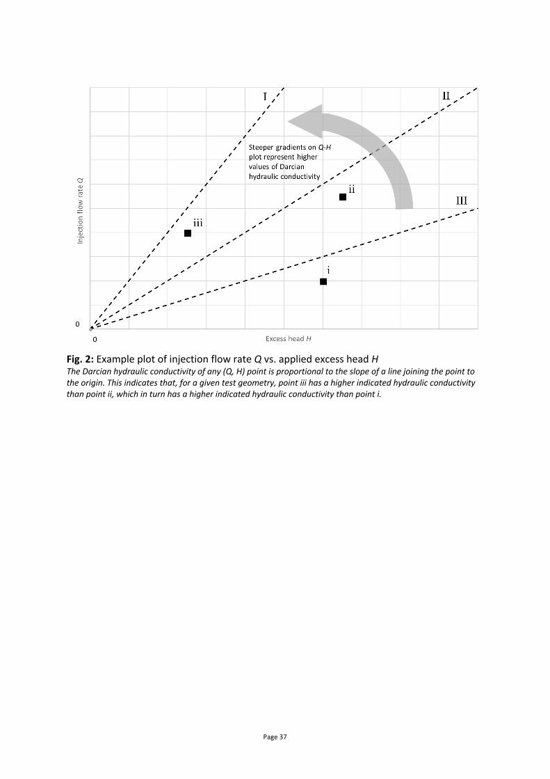
Page 37

Fig. 2: Example plot of injection flow rate Q vs. applied excess head H The Darcian hydraulic conductivity of any (Q, H) point is proportional to the slope of a line joining the point to the origin. This indicates that, for a given test geometry, point iii has a higher indicated hydraulic conductivity than point ii, which in turn has a higher indicated hydraulic conductivity than point i.

Page 38

a. Type 1: Zero water take Effectively zero water injection rate at all excess heads

b. Type 2: Linear Q-H relationship with small hysteresis loop Injection flow rate and excess head have an approximate linear relationship (including the line to the origin), with only a small hysteresis between the ascending and descending test phases

c. Type 3: Non-linear (under-proportional) Q-H relationship with small hysteresis loop Injection flow rates are not linearly related to excess head, and the apparent hydraulic conductivity reduces as excess head increases, with only a small hysteresis between the ascending and descending test phases Fig. 3: Q-H plots for conventional packer test responses

Page 39

d. Type 4: Non-linear (over-proportional) Q-H relationship with small hysteresis loop Injection flow rates are not linearly related to excess head, and the apparent hydraulic conductivity increases as excess head increases, with only a small hysteresis between the ascending and descending test phases

e. Type 5: Non-linear (over-proportional) Q-H relationship with large hysteresis loop Apparent hydraulic conductivity increases for each phase, including descending heads, this gives a significant hysteresis loop, where hydraulic conductivity is greater in the descending A2, B2 phases compared to the ascending A1, B1 phases

f. Type 6: Non-linear (under-proportional) Q-H relationship with large hysteresis loop Apparent hydraulic conductivity decreases for each phase, including descending heads, this gives a significant hysteresis loop, where hydraulic conductivity is lower in the descending A2, B2 phases compared to the ascending A1, B1 phases Fig. 3: Q-H plots for conventional packer test responses

Page 40

g. Type 7: Water take limited by equipment pumping rates with low excess head achieved Injection rate quickly reaches close to the maximum injection flow rate Qmax for the test equipment, which is not able to establish an excess head in the test section Fig. 3: Q-H plots for conventional packer test responses

Page 41

a. Type 8: Sudden excess head drop to zero Injection flow rate shows a conventional Q-H relationship up to a given head, at which point the flow rate increases rapidly and the excess head drops to almost zero

b. Type 9: Flow rate initiates at significant non-zero excess head Injection flow rate is effectively zero at lower excess heads, and increases suddenly under the higher heads of later phases

c. Type 10: Excess head does not build until significant non-zero flow rate Excess head is effectively zero at lower injection rates, and increases suddenly under the higher flow rates of later phases Fig. 4: Q-H plots for non-conventional packer test responses

Page 42

Fig. 5: Example plots of packer test analysis (data from Table 3)

Page 43

Fig. A1: Correlation between Lugeon Coefficient and hydraulic conductivity (Borehole diameter = 76 mm; excess head in test section 1000 kPa)

(a) pressure transducer within the test section (double packer test shown)

(b) pressure gauge in the above ground injection pipework (double packer test shown)

Fig. A2: Measurement of applied excess head in packer test