NoSQL Databases and Cassandra

Pratham Solanki ULB Student Id: 000474971

Braulio Blanco ULB Student Id: 000475854

Advanced Databases

Prof. Esteban Zimanyi

December 2018

Table of Contents

I. Introduction 4

II. Databases 4

2.1. NoSQL Databases 4

2.1.1. Need for NoSQL Databases 4

2.1.2. NoSQL emergence 4

2.1.3. Aggregate orientation 4

2.1.4. Definition 5

2.1.5. Types and examples 5

2.1.5.1. Key Value 5

2.1.5.2. Documental DB 6

2.1.5.3. Column-Family 6

2.1.5.4. Graph DB 6

III. Cassandra Database 7

3.1. History 7

3.2. Data Model 8

3.2.1. Clusters 8

3.2.2. Keyspaces 8

3.2.3. Column Families 9

3.2.4. Column 9

3.2.5. Super Columns 10

3.2.6. Wide Rows and Skinny Rows 10

3.2.7. Datatypes supported 10

3.3. Architecture 11

3.3.1. Peer to Peer 11

3.3.2. Gossip and Failure detection 11

3.3.3. Partitioning and Replication 11

3.3.4. Commit Logs, Memtables and SSTables. 12

3.3.5. SSTables 12

3.3.6. Eventual Consistency 13

3.3.7. Hinted Handoff 13

3.3.8. Consistency Level 13

3.3.9. Tombstones 14

3.3.10. Compaction 14

3.3.11. Bloom Filters 15

3.3.12. Caching 15

3.3.13. Partition Summary and Partition index 15

3.3.14. Compression Offset map 15

3.4. Reading and Writing Lifecycle 15

3.4.1. Writing data: 15

3.4.2. Reading data 16

3.4.3. Updating and deleting data 17

3.4.4. Maintaining data 17

3.5. Cassandra Query Language CQL 18

3.5.1. Create Keyspace 18

3.5.2. Create Table 18

3.5.3. Insert Into 18

3.5.4. Select Table 18

4. Use case study 18

5. Conclusion 28

6. References 29

I. Introduction

This project explains briefly how does the NoSQL databases appeared and the

different main types of this databases we have, but the focus is the Cassandra

technology, how it works and the performance analysis of Cassandra with a SQL

Relational Database.

II. Databases

2.1. NoSQL Databases

2.1.1. Need for NoSQL Databases

In the last years there are new trends that relational databases or SQL databases

that have not been able to overcome effectively. Some of these new trends are:

Big data, Heterogeneous and multiplicity in connectivity, P2P Knowledge, High

Concurrence, Data diversity, Cloud-grid.

2.1.2. NoSQL emergence

The term NoSQL first made its appearance in the late 90s as the name of an open-

source relational database. Led by Carlo Strozzi, this database stores its tables as

ASCII files, each tuple represented by a line with fields separated by tabs. This

database doesn’t use SQL as its query language, instead it used scripts that can be

combined into the usual UNIX pipelines (Sadalage & Fowler, 2013). After, in the

meetup organized by Johan Oskarsson in San Francisco (2009), and by this time,

there were several projects that were working in database storage inspired on

BigTable (Google) and Dynamo (Amazon) and this meeting was a good moment

that would have these projects to present its works, after he asked in a social

network channel the suggestions for the name of the meetup, the result was

named as NoSQL. But the intension was to name only the event, but this later

become in the name of the technology trend. When the trend become popular the

main characteristics of this kind of databases was schema-free, easy replication

support, support of large-scale databases and eventually consistent but not ACID

(Relational databases).

2.1.3. Aggregate orientation

Aggregation is a collection of related objects that should be treated as a unit. It is

represented like a tree, and there is a main node (or multiples first level nodes)

that has one or more nodes that could have the same distribution in deep, like an

xml file of an order and its detail. In the other hand, aggregations present in a more

compressible understandable way. For this reason, relational databases are called

aggregate-ignorant (Sadalage & Fowler, 2013). In NoSQL databases, only graph

databases are aggregate-ignorant. One of the weakness of aggregation is when we

are trying to analyze deeper data for example considering the main and

intermediate data in a range of time of as a subset of another object, in these cases

for obtaining the data could be more complex.

2.1.4. Definition

NoSQL refers to “Not only SQL”

databases and has been

developed based on the new

trends of modern applications

and requirements. Usually are

non-relational, distributed,

open source projects and

scalable.

Martin Fowler (Sadalage &

Fowler, 2013) uses the phrase of

polyglot persistence,

referencing to using different

data store in different

circumstance, and the

organizations must to learn when to use each kind of database (Relational or non-

relational) according to business needs instead of trying to unified in a single

technology. According to the CAP Theorem or Brewers Theory, in a distributed

system we only have the option of choose two of these three options.

2.1.5. Types and examples

2.1.5.1. Key Value

Key Value

databases are

strongly aggregate-

oriented because

are mainly built by

aggregations. Each

aggregate has a key that we use for getting the data. It is the unique way to

get the value. In this type of database, the aggregate is opaque and this allow

us to store whatever we want, only with size limits restrictions. Some key-

value database projects are: Windows Azure Blob Azure, Windows Azure Table

Storage, Windows Azure Cache, Redis, Memcached, Riak, Dynamo (Amazon),

Voldemort, Membase, Tokyo Cabinet, mem cached, hazelcast.

Figure 2.Key/Value database model Source: https://neo4j.com/

Figure 1. CAP Theorem Source: Own elaboration based in different sources detailed in

references

2.1.5.2. Documental DB

Also, this type of database is strongly-

aggregate aggregate-oriented. It consists

in a lot of aggregations that has a Key for

getting the data, but in contrast with

key/value databases, we also can get the

data from other fields different than the

key or ID. Also allows us to see the

structure in the aggregation, and defines

the structure and type of data that could

be allowed. Some documental databases

are: MongoDB, Raven DB, Couch DB.

2.1.5.3. Column-Family

This database was created by

Google in a project called

BigTable. The name makes us to

wonder in table structure, but it is

more like a two-level map. This is

often referred as column stores.

The first key is usually described

as the row identifier and the

second level is referred to as columns. This database organizes the columns

into columns families. The column family is a group of rows that each row

represents a column and its value. So, a row in the relational model should be

represented in this database like the union of the first level row and its column

families and its values in the second level. After Bigtable, there are others

highly spread projects that use this data model: Cassandra, HBase, Hypertable,

SimpleDB (AmazonWS).

2.1.5.4. Graph DB

Most of the NoSQL projects are

conceptualized for running on

clusters, therefore, manage a large

amount of data with simple

relations. Graph databases are

designed differently where there is

a lot of relations that connects

small amount of data. Some Graph

Figure 6. Column Family database model Source: own elaboration based on

http://alexminnaar.com

Figure 5. Document database model Source: https://docs.mongodb.com

Figure 7. Graph database model Source: Own elaboration based on

http://neo4j-contrib.github.io

Databases are: Neo4j, Infinite Graph, Titan, Cayley, FlockDB (Twitter).

III. Cassandra Database

Apache Cassandra is a free and open-source, distributed, wide column store, NoSQL

database management system designed to handle large amounts of data across many

commodity servers, providing high availability with no single point of failure.

Cassandra offers robust support for clusters spanning multiple datacenters,[1] with

asynchronous masterless replication allowing low latency operations for all clients.

3.1. History

● 2007: Facebook engineers Avinash Lakshman and Prashant Malik develop Cassandra

to power Facebook’s inbox search feature using large datasets across multiple

servers. They name their database after the Trojan mythological prophet Cassandra

- with classical allusions to a curse on an oracle. Lakshman’s presentations and the

team’s LADIS (Large Scale Distributed Systems) paper generate excitement in the

distributed systems community.

● 2008, July: Facebook releases Cassandra as an open source project on (now defunct) Google Code.

● 2008, Nov-Dec: Rackspace hires distributed systems engineer Jonathan Ellis with a mandate to build a next-generation scalable database. After evaluating the extant open source projects, he forms a small Cassandra group at the company.

● 2009, Jan: Facebook, Lakshman, and Malik contribute Cassandra to the Apache Software Foundation, where it becomes an Apache Incubator project.

● 2009, Mar: Jonathan Ellis becomes the first new committer to Cassandra in the Apache Incubator. His blogging activity and omnipresence on IRC make him the face of Cassandra to the community.

● 2009, Apr: Ellis is contacted by John Vrionis of Lightspeed Ventures, who asks him if he’s thought about starting a company around Apache Cassandra. Ellis had indeed begun to have these thoughts, but wasn’t quite ready to pull the trigger.

● 2009, May: Twitter engineer Johan Oskarsson announces a conference for scalable databases in San Francisco. Cassandra committer Eric Evans suggests calling this a “NoSQL”

conference, and the term sticks. ● 2009, Nov: Comcast engineers respond to a Cassandra users survey conducted by Ellis. They

evaluated Cassandra positively for a data-intensive project, but corporate policy required having a company behind it that they could call for support. Ellis takes this as the sign he was looking for to start his own company based on Apache Cassandra.

● 2010, Feb-Mar: Ellis convinces fellow Rackspace engineer Matt Pfeil to quit his job and cofound Riptano with him in Austin to commercialize Apache Cassandra.

● 2010, Apr: Cassandra graduates from the incubator and becomes a top-level project of the Apache Foundation, with Jonathan Ellis as project chair.

● 2010, July: Amid competition from multiple interested VC firms, Lightspeed Ventures leads Riptano’s Series A funding round.

● 2011, Jan: Pfeil and Ellis decide to change Riptano’s name to DataStax.

● 2011, May: Ellis and Pfeil hire college football player-turned-tech entrepreneur Billy

Bosworth as CEO to help manage the company’s hypergrowth and to get another round of investment, which was led by Crosslink Capital.

● 2011: The NoSQL data management market explodes, with hundreds of start-ups appearing in the space.

● 2011, Oct: Apache Cassandra 1.0 is released, and so is Version 1 of DataStax Enterprise, the first integrated data platform with built-in analytics powered by Hadoop running on top of Apache Cassandra.

● 2012, Aug: University of Toronto researchers studying NoSQL systems conclude that "In terms of scalability, there is a clear winner throughout our experiments. Cassandra achieves the highest throughput for the maximum number of nodes in all experiments" although "this comes at the price of high write and read latencies." Ellis is determined to fix this.

● 2012-2013: DataStax enters accelerated development and Cassandra awareness mode, significantly advancing Cassandra’s capabilities and spreading the message about the power of Cassandra-based NoSQL data management throughout the tech world. They achieve adoption at many of Silicon Valley’s top tech companies, including Apple, Netflix, and Twitter.

● 2013-2017: DataStax goes into growth mode, taking on a number of big-name customers, including Sony, eBay, Walmart, and FedEx, and going from plucky little startup to the cloud database market leader. DataStax engineers continue to develop Cassandra, making 85% of the code commits and accelerating Cassandra’s evolution through V. 3.11.

● 2018, May: DataStax releases DataStax Enterprise 6, which is 2 times faster than open source Apache Cassandra while eliminating significant operational complexity.

3.2. Data Model

3.2.1. Clusters Cassandra database is distributed over several machines that operate together. The

outermost container is known as the Cluster. For failure handling, every node contains a

replica, and in case of a failure, the replica takes charge. Cassandra arranges the nodes in a

cluster, in a ring format, and assigns data to them.

3.2.2. Keyspaces Keyspace is the outermost container for data in Cassandra. The basic attributes of a

Keyspace in Cassandra are:

- Replication factor − It is the number of machines in the cluster that will receive copies

of the same data.

- Replica placement strategy − It is nothing but the strategy to place replicas in the ring.

We have strategies such as simple strategy (rack-aware strategy), old network

topology strategy (rack-aware strategy), and network topology strategy (datacenter-

shared strategy).

- Column families − Keyspace is a container for a list of one or more column families. A

column family, in turn, is a container of a collection of rows. Each row contains ordered

columns. Column families represent the structure of your data. Each keyspace has at

least one and often many column families.

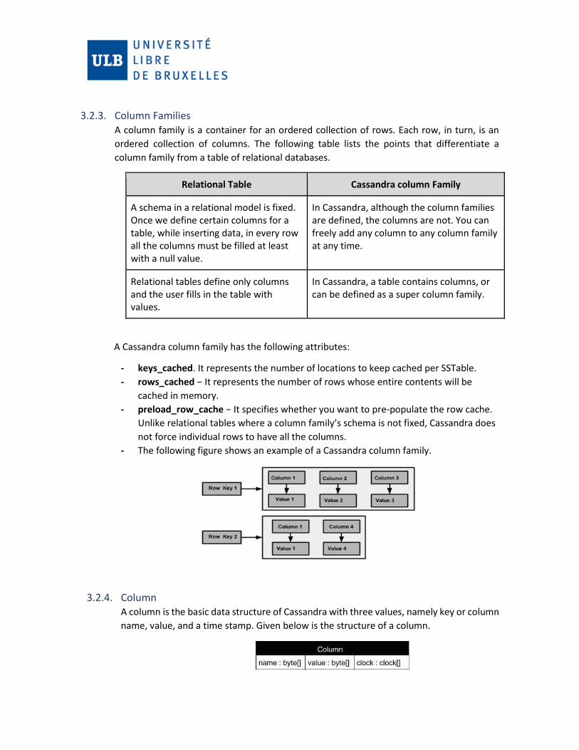
3.2.3. Column Families A column family is a container for an ordered collection of rows. Each row, in turn, is an

ordered collection of columns. The following table lists the points that differentiate a

column family from a table of relational databases.

Relational Table Cassandra column Family

A schema in a relational model is fixed. Once we define certain columns for a table, while inserting data, in every row all the columns must be filled at least with a null value.

In Cassandra, although the column families are defined, the columns are not. You can freely add any column to any column family at any time.

Relational tables define only columns and the user fills in the table with values.

In Cassandra, a table contains columns, or can be defined as a super column family.

A Cassandra column family has the following attributes:

- keys_cached. It represents the number of locations to keep cached per SSTable.

- rows_cached − It represents the number of rows whose entire contents will be

cached in memory.

- preload_row_cache − It specifies whether you want to pre-populate the row cache.

Unlike relational tables where a column family’s schema is not fixed, Cassandra does

not force individual rows to have all the columns.

- The following figure shows an example of a Cassandra column family.

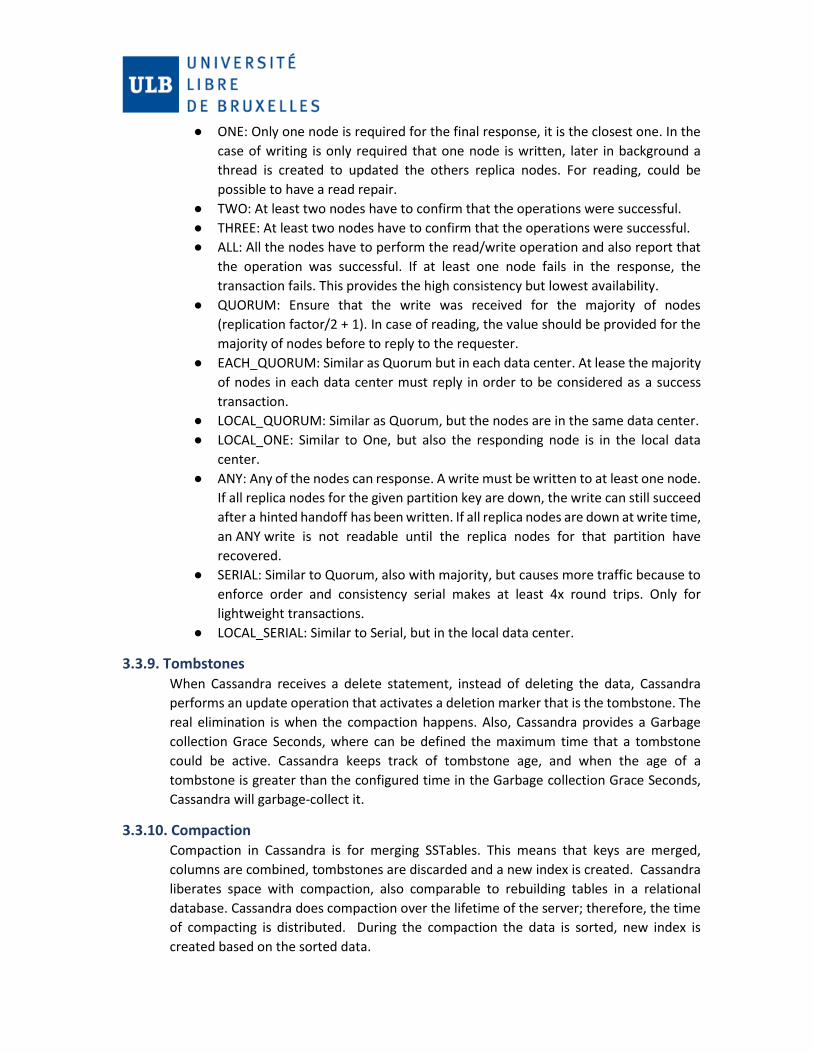
3.2.4. Column A column is the basic data structure of Cassandra with three values, namely key or column

name, value, and a time stamp. Given below is the structure of a column.

3.2.5. Super Columns

A super column is a special column; therefore, it is also a key-value pair. But a super column

stores a map of sub-columns.

Generally, column families are stored on disk in individual files. Therefore, to optimize

performance, it is important to keep columns that you are likely to query together in the

same column family, and a super column can be helpful here. Given below is the structure

of a super column.

3.2.6. Wide Rows and Skinny Rows A Row in a Table can be called as Wide or Skinny depending on the no of Columns in a

Table. A Row can be called Wide row if the table contain Columns in Thousands or Millions.

Primary Key associated with Wide Row can can be called as Compound Key as it involves

2 Keys.

3.2.7. Datatypes supported

Data Type

Constants Description Data Type

Constants Description

Ascii Strings Represents ASCII character string

Inet Strings Represents an IP address, IPv4 or IPv6

Bigint Bigint Represents 64-bit signed long

Int Integers Represents 32-bit signed int

Blob Blobs Represents arbitrary bytes Text Strings Represents UTF8 encoded string

Boolean Booleans Represents true or false timestamp

integers, strings

Represents a timestamp

Counter Integers Represents counter column Timeuuid

Uuids Represents type 1 UUID

Decimal integers, floats

Represents variable-precision decimal

Uuid Uuids Represents type 1 or type 4

Double Integers Represents 64-bit IEEE-754 floating point

Varchar Strings Represents uTF8 encoded string

Float integers, floats

Represents 32-bit IEEE-754 floating point

Varint Integers Represents arbitrary-precision integer

Collection Types:

Collection Description

List A list is a collection of one or more ordered elements.

map A map is a collection of key-value pairs.

Set A set is a collection of one or more elements.

3.3. Architecture

3.3.1. Peer to Peer In many relational databases architectures that are deployed in a cluster environment,

follows the master-slave architecture, that means that the master receives the request

and replicates the information to the slaves, but this represents a single point of failure. In

the case of Cassandra, the distribution model is pear-to-pear, in consequence there is no

master node, and the request can be received for any node in the cluster, for this reason

if a node fails, the system can still alive to attend requests.

3.3.2. Gossip and Failure detection Cassandra uses Gossip protocols for failure detection. According to the period stablished

on the configuration each node (initiator) selects randomly another node in the ring and

creates a session with this node (Friend node), using the Gossiper component. Then the

initiator sends a GossipDiggestMessage to the friend node and this one reply with a

GosspipDiggestAckMessage to inform that is still active. After receive the AckMessage, the

initiator sends a GosspipDiggestAckMessage to the selected node. If the Gossiper detects

that one node is not active, the Gossiper mark the node as dead in its local list. It occurs

with all the nodes in order to gather information of all the other nodes.

Also, Cassandra implements the Phy Accrual Failure Detection for supporting failure

detection. This method doesn’t mark a node as active or inactive because the heartbeat,

this method uses a suspicion level, that means that is a value between active and inactive.

The calculation of the Phy value considers the time that is increasing since the last alive

report that receives, and this in a logarithmic function. The threshold to decide if a Phy is

a failure is configurable.

3.3.3. Partitioning and Replication The purpose of partitioning is to distribute the data across the nodes. The partitioning

algorithm can be defined in the configuration. Cassandra provides three groups of

partitioners: Random partitioner, murmur3 partitioner, order-preserving partitioner (that

includes order-preserving partitioner, collating order-preserving partitioner and Byte-

Ordered partitioner). The random partitioner uses MD5 hash applied to a key to get a

BigIntegerToken to determine which place will be the key in the ring. The main

disadvantage is that the queries are inefficient, because have to get from different

locations. And the returned data will be no sorted. Cassandra creates an alternative to this

and make it as its default partitioner (Random Partitioner was default until 1.1 version,

including) the Murmur3Partitioner. Murmur3 is faster than the first version of Random

partitioner, using MurmurHash function that is a random function also. Thirdly, the order-

preserving partitioner creates a UTF-8 string based on the key, for this case, the keys are

stored sorted, the disadvantage of this partitioner is that some nodes could be very dense

and some nodes could have only few values. For solving this problem, it is necessary that

the administrator balance the nodes periodically. A variant of this partition is the Collation

Order-Preserving, this uses the collation of English locale (EN_US) and works with UTF-8

strings also. An optimization is the Byte-Ordered partitioner, which also preservers the

order of the data as way bytes, this doesn’t validate that keys are strings as the two

previous does.

3.3.4. Commit Logs, Memtables and SSTables. Is a log that stores all the operations. It is used for crash-recovery. If the commit of a write

transaction is written in the commit log, so it is considered as a successful transaction.

After a value is written in the Commit Log, it should be written in Memtables. If the

memtable is full, the data is flushed into SSTables on disk. The commit log is purged after

the flush.

Memtables are structures that store the data in memory, and keep it until it reaches the

threshold, if the threshold is reached, the contents of the memtables are flushed to disk

in a SSTable (Sorted Strings table) file using sequential I/O instead of random I/O, and it is

one of the reasons of the high performance. There are less I/O operations.

Figure 6. SSTables and Index files Source: https://www.igvita.com/

3.3.5. SSTables Partitions has multiple SSTables, and each SSTable contents: Data, Primary Index list,

bloom filter, compression information, statistics, digests, CRC, SS Table Index Sumary, SS

Table of Contents and Secondary index.

● Data (Data.db): The SSTable data.

● Primary Index (Index.db): Index of row keys that had pointers to the positions in

the Data.db file.

● Bloom filter (Filter.db): Structured stored in memoty that checks if the data exists

in the memtable before to access the SSTables on disk.

● Compression information (CompessionInfo.db): All the compression information.

● Statistics (Statistics.db) statistics of the metadata about the content of the

SSTable.

● Digest (Digest.cr32, Digest.adler32, Digest.sha1): Is the file for consistency check

of the data file, the checksum.

● CRC (CRC.db): File that holds the CR32 for the chunks in a compressed file.

● SSTable Index Summary (SUMMARY.db): Part of the index information that is

stored in memory.

● SSTable of Contents (TOC.txt): A file that includes all the components.

● Secondary Index (SI_.x.db): List of secondary indexes. And could exists zero, one

or more than one Secondary Index files.

3.3.6. Eventual Consistency A transaction must leave a database in a legal state when it ends, that is called consistency.

Cassandra according to CAP theorem, emphasizes in Availability and Partition Tolerance

as we mentioned before. In the case of Consistency, Cassandra can’t ensure string

consistency and it relies in eventual consistency. Eventual consistency is the degree of

consistency of the system, and this is represented with the following formula: W+R<=N,

where W is the number of replicas that should report as successful before to report the

transaction as success, R means the number of replicas that are contacted when a data

object is acceded in a read operation; and N is the number of nodes that store replicas of

the data. On the other hand, a strong consistency is: W+R > N.

3.3.7. Hinted Handoff It is a mechanism that Cassandra uses for ensure the general availability in the ring where

there is a network problem or not availability of a node. If a write request should be

attended for a node that for different reasons can’t attend the request, the node that takes

the first contact creates a hint or reminder that this node have a value that should be

delivered to the other node. When the other node comes back online, the first receiver

hand off the hint to the destination node. This procedure to attend the writing request is

similar to Java Message Service (JMS).

In case of the node remains offline for a long time, and many nodes have lots of hints for

handing off to this vulnerable node, the node will receive many requests almost at the

same time, and could cause that the node could fall again. For this reason, Cassandra

allows to avoid the use of hinted hand-off or reduce the use of this. The hand-off happens

after the consistency level has been met, except for the case of the ANY consistency level

that only requires that the hint has been created.

3.3.8. Consistency Level In Cassandra, the queries can specify how much consistency is required. A higher

consistency means that more nodes needs to reply the success of the transaction before

consider reply to the sender with the result. In the case of two or more nodes reply with a

different value, the timestamp value is revised, and the most recent is taken. After this,

Cassandra will update all the inconsistent values, this last process is called “read repair”.

There are four consistency levels: ONE, TWO, THREE, ALL, EACH_QUORUM, QUORUM,

LOCAL_QUORUM, LOCAL_ONE, ANY, also for reading is added: SERIAL and LOCAL_SERIAL.

● ONE: Only one node is required for the final response, it is the closest one. In the

case of writing is only required that one node is written, later in background a

thread is created to updated the others replica nodes. For reading, could be

possible to have a read repair.

● TWO: At least two nodes have to confirm that the operations were successful.

● THREE: At least two nodes have to confirm that the operations were successful.

● ALL: All the nodes have to perform the read/write operation and also report that

the operation was successful. If at least one node fails in the response, the

transaction fails. This provides the high consistency but lowest availability.

● QUORUM: Ensure that the write was received for the majority of nodes

(replication factor/2 + 1). In case of reading, the value should be provided for the

majority of nodes before to reply to the requester.

● EACH_QUORUM: Similar as Quorum but in each data center. At lease the majority

of nodes in each data center must reply in order to be considered as a success

transaction.

● LOCAL_QUORUM: Similar as Quorum, but the nodes are in the same data center.

● LOCAL_ONE: Similar to One, but also the responding node is in the local data

center.

● ANY: Any of the nodes can response. A write must be written to at least one node.

If all replica nodes for the given partition key are down, the write can still succeed

after a hinted handoff has been written. If all replica nodes are down at write time,

an ANY write is not readable until the replica nodes for that partition have

recovered.

● SERIAL: Similar to Quorum, also with majority, but causes more traffic because to

enforce order and consistency serial makes at least 4x round trips. Only for

lightweight transactions.

● LOCAL_SERIAL: Similar to Serial, but in the local data center.

3.3.9. Tombstones When Cassandra receives a delete statement, instead of deleting the data, Cassandra

performs an update operation that activates a deletion marker that is the tombstone. The

real elimination is when the compaction happens. Also, Cassandra provides a Garbage

collection Grace Seconds, where can be defined the maximum time that a tombstone

could be active. Cassandra keeps track of tombstone age, and when the age of a

tombstone is greater than the configured time in the Garbage collection Grace Seconds,

Cassandra will garbage-collect it.

3.3.10. Compaction Compaction in Cassandra is for merging SSTables. This means that keys are merged,

columns are combined, tombstones are discarded and a new index is created. Cassandra

liberates space with compaction, also comparable to rebuilding tables in a relational

database. Cassandra does compaction over the lifetime of the server; therefore, the time

of compacting is distributed. During the compaction the data is sorted, new index is

created based on the sorted data.

3.3.11. Bloom Filters

These filters help to Cassandra to determine if a value corresponds to a set. It is non-

deterministic because to get a false-positive answer, but never a false-negative. Bloom

filters maps the data into a bit array condensing the data into a string. These filters are

stored in memory and allows to avoid disk access, that improves the performance of the

queries. If the filters indicate that the element doesn’t exists, it doesn’t exist. In the other

hand if the filter indicate that the element exists, its not a guarantee that it exists, so, is

required to access to the disks for looking the data.

3.3.12. Caching For caching, the environment requires considerable memory. Cassandra provides two

primary caches: Row cache and key cache. In the first case, the rows are stored completely,

including all the columns, in the other case, only the keys and the reference to the location.

3.3.13. Partition Summary and Partition index The partition summary stores in memory a sampling of the partition index, and a partition

index contains all the partitions keys. If the size of the summary is set in 50, the partition

summary will save each 50 rows, the location of the partition key. The partition index

stores in disk all the locations (offset) of the keys and with this information, the

compression map is used for locate the key in the disk.

Figure 6. SSTables and Index files Source: https://avdeo.com/2015/06/01/cassandra-2-0-architecture/

3.3.14. Compression Offset map This lists stores in memory points to the exact location on disk. In this map is compressed

the offsets, and when is required to access to the disk this information must be

uncompressed.

3.4. Reading and Writing Lifecycle

3.4.1. Writing data: There is no update statement in Cassandra. The update is solved using Insert statement

with an existing key. If the update contains columns that there is no in the current

structure, these columns will be added. Writing doesn’t support transactions, in

consequence, if a user sent a group of statements, if an error occurs, the sender has to

roll-back manually.

The process of writing starts when Cassandra writes in the commit log and then in the in

the memtable. When the memtable reach the threshold, it is put in a queue for being

flushed into the SSTables in the disk. Each commit log maintains an internal bit flag for

indicating if the memtable require to be flushed. If the data exceeds the threshold,

Cassandra blocks writes until the next flush success. After this, a partition index is created.

This index maps the tokens to the disk location.

It is important to mention that each table has its own Memtable and one or more SSTables,

but the commit log is a shared component. SSTables are inmutable, after the flushed

occurred. Data in the commit log is purged after the flushing.

Figure 6. Writing of flow Source: https://docs.datastax.com/

3.4.2. Reading data Clients in reading can connect to any node in the cluster. If the node doesn’t have the data,

this node acts like the coordinator between the destination and the sender. The

coordinator locates the destination node according the token ranges. Cassandra uses the

Bloom filter as first resource in order to know if the data doesn’t exist.

For the response, Cassandra looks the data in different levels and if there is the data,

returns to the requester the results. First the node checks the memtable, then the row

cache if it is enabled and then the bloom filter, then the partition key cache, if there is a

partition key, goes directly to the compression offset, else, checks the partition summary

and the corresponding partition index and consequently the compression offset. After

reading the compression offset, locates the data from the SSTables on the disk.

Figure 6. Reading Flow Source: https://docs.datastax.com/

3.4.3. Updating and deleting data As we mentioned before, an update statement is treated as an insert statement that has

an existing key. So, there will be multiple versions of the same key in different rows. If

during the compaction Cassandra found two or more versions of the same data, only the

most recent version to the new SSTable. In the case of a deletion statement, as we

mentioned before, actives the tombstone marker. In a distributed system, the marker is

distributed to the other replica nodes.

3.4.4. Maintaining data Cassandra have to clean the data because the multiples rows that appeared because

updating and deleting. In the case of update rows, remove earlier versions and for

deleting, removing the rows marked with the tombstone mark.

3.5. Cassandra Query Language CQL

For this report we refer the official documentation for Cassandra Query Language (datastax,

s.f.). In this section, we only are considering four statements that we are using in our

implementation of Cassandra: Create Keyspace, Create table, Insert into and Select From.

3.5.1. Create Keyspace

3.5.2. Create Table

3.5.3. Insert Into

3.5.4. Select Table

4. Use case study

For our Cassandra implementation we pick the data from the U.S.A. government page

(USA Data.gov, s.f.) that corresponds to Crime Data and we create a Crime Table and

a java program to insert and query the data to the databases.

For this work we are considering two databases systems for comparison: Cassandra

and MS SQL Server that are deployed as service in a local Docker server. For the

present work we create two environments; the first environment was implemented

for comparing the performance between Cassandra and SQL Server and the second

environment was implemented for comparing the performance between Cassandra

with different configurations.

• Environment 01: In this first environment we had created a java client that reads

records from the csv crime data and inserts/read it into/from Cassandra using

the datastax driver, the start time and end time are registered for comparison,

after this the same data is inserted /read it into/from SQL Server using the

java.sql connector and also the times are registered. The java client ran 10 times

per each server, each time with different amount of data. We have only created

a table in Cassandra and the equivalent one table in SQL, this is because

according the Cassandra Architecture, it is oriented to be redundant in data

according to the queries and in a natural way doesn’t implement table relations.

Environment Test # 01

Docker server

SQL ServerCassandra

(Replication Factor =1, Nodes =1)

ClientJVM

Cassandra Connector(com.datastax.driver.core)

SQL Connector

(java.sql.Connection)

.csv ReaderClient

a) Configuration of Cassandra environment:

o Install docker and get Cassandra image. After installing docker we can get the

Cassandra image in order to create the server. In the command line execute the

following command.

> docker pull Cassandra

o After the image of Cassandra has been downloaded, we create the service.

> docker run --name cassandra -p 127.0.0.1:9042:9042 -p 127.0.0.1:9160:9160 -d cassandra

o When the server has been created, it automatically starts the server. For

executing CQL instructions, we have to get the bash of Cassandra with the

following command.

> docker exec -it cassandra bash

o To start the client of CQL we execute the following command.

> cql sh

o For creating the keyspace, we use the following command.

# CREATE KEYSPACE Crime WITH REPLICATION = { 'class' : 'SimpleStrategy', 'replication_factor' :

1 };

o For using the keyspace, we have to change of keyspace with the following

command.

# USE crime;

o For creating the column family, we use the following command. As we can see

the create table statement is similar to T-SQL Statement, the main difference

are the datatypes.

# CREATE TABLE crimeReport (

drNumber int,

dateReported timestamp,

dateOcurred timestamp,

timeOcurred int,

areaid int,

reportingDistrict int,

moCodes varchar,

victimAge int,

victimSex varchar,

premiseCode int,

weaponCode int,

crimeCode set<varchar>,

address varchar,

locationX decimal,

locationY decimal,

upload_date timestamp,

PRIMARY KEY (drNumber)

);

o The java program creates records based on the csv file with the following insert

structure as an example. As we can see the insert statement is similar to T- SQL

statement.

# INSERT INTO crimeReport (drNumber,dateReported,dateOcurred, timeOcurred, areaid,

reportingDistrict, moCodes, victimAge, victimSex, premiseCode, weaponCode, crimeCode,

address, locationX, locationY, upload_date)

VALUES (1208575,'2013-03-14 00:00:00','2013-03-11 00:00:00',1800,12,1241,'0416 0446 1243

2000',30,'001',502, 120, {'510',’504’},'6300 BRYNHURST AV',33.9829, -118.3338,'2018-12-03

01:28:34');

o The java program query records according to a given ID. As we can see the insert

statement is similar to T- SQL statement.

# SELECT * FROM crimeReport WHERE drNumber= ‘drNumber’

b) Configuration of SQL Server environment:

o In the command line, using the docker service, get the SQL Server image.

> docker pull mcr.microsoft.com/mssql/server:2017-latest

o After the image of SQL Server has been downloaded, we create the service.

> docker run -e "ACCEPT_EULA=Y" -e "SA_PASSWORD=P@ss" -p 1433:1433 --name sql1 -d

mcr.microsoft.com/mssql/server:2017-latest

o When the server has been created, it automatically starts the server. For

executing SQL instructions, we have to get the bash of SQL Server with the

following command.

> docker exec -it sql1 "bash"

o To start the client of SQL we execute the following command.

> /opt/mssql-tools/bin/sqlcmd -S localhost -U SA -P 'P@ss'

o For creating the database, we use the following command.

# CREATE DATABASE Crime

ON

( NAME = Crime_dat,

FILENAME = 'C: \MSSQL\DATA\crimedat.mdf', SIZE = 100MB, MAXSIZE = 1GB, FILEGROWTH =

15% )

LOG ON

( NAME = Crime_log,

FILENAME = 'C: \MSSQL\DATA\crimelog.ldf', SIZE = 5MB, MAXSIZE = 25MB, FILEGROWTH =

5MB ) ;

;

o For using the database, we use the following command.

# USE crime;

o For creating the table, we use the following command.

# CREATE TABLE crimeReport(

drNumber int,

dateReported date,

dateOcurred date,

timeOcurred int,

areaid int,

reportingDistrict int,

moCodes varchar(200),

victimAge int,

victimSex varchar(1),

premiseCode int,

weaponCode int,

crimeCode varchar(200),

address varchar(200),

locationX decimal(18,0),

locationY decimal(18,0),

upload_date date,

PRIMARY KEY (drNumber)

);

o The java program creates records based on the csv file with the following insert

structure as an example. As we can see the insert statement is similar to T- SQL

statement. As we mention in the previous section, Cassandra performs an insert

operation if she doesn’t find the key and it updated the information with the

key already exists, for this reason the corresponding comparison in SQL server,

for each row we are querying the database and checking if it exists or not, in

the case that the row exists, the java program performs an update statement,

otherwise, performs an insert statement.

# INSERT INTO crimeReport (drNumber,dateReported,dateOcurred, timeOcurred, areaid,

reportingDistrict, moCodes, victimAge, victimSex, premiseCode, weaponCode, crimeCode,

address, locationX, locationY, upload_date)

VALUES (1208575,'2013-03-14 00:00:00','2013-03-11 00:00:00',1800,12,1241,'0416 0446 1243

2000',30,'001',502, 120, '510-504’,'6300 BRYNHURST AV',33.9829, -118.3338,'2018-12-03

01:28:34');

o The java program query records according to a given ID.

# SELECT * FROM crimeReport WHERE drNumber= ‘drNumber’

c) Test Plan:

We prepare the software to run 10 test cases, each with different number of

records, each one duplicates the amounts of records of the previous test case as we

can see in the following table. This test case set was executed for inserting and for

querying both databases. In total for this environment the java program runs 40

times.

Case N° Number of Records

Case N° Number of Records

1 100 6 3,200

2 200 7 6,400

3 400 8 12,800

4 800 9 25,600

5 1,600 10 51,200

d) Results:

In the following chart we can see the performance when Cassandra inserts/updates

the data considerably faster than SQL Server. Both servers are performing a query

of the database for searching the key and according to this, performs an insert or

update. In the case of SQL server this procedure is done manually for the java client.

As we can see Cassandra only performs the insert/update operation for the

maximum number of records (51,200) in 124.60 seconds, approximately 7% of the

time consumed by SQL Server.

In the other hand we have the performance when both select the data. As we can

see in the following chart, the performance of SQL Server is better than Cassandra.

SQL server consumes 66% of the time of Cassandra.

• Environment 02: In this environment we use the java client described in the

previous part, this component read data from the csv crime file and inserts/read

it into/from Cassandra. The java client ran 10 times per each server

configuration, each time with different amount of data. We use the same

schema that was created in the first environment.

Environment Test #02

Client

JVM Client .csv Reader

Cassandra Connector(com.datastax.driver.core)

Docker and docker compose server

Cassandra Node1(Replication Factor =2)

Cassandra Node2(Replication Factor =2)

Cassandra Node3(Replication Factor =2)

Cassandra Node4(Replication Factor =2)

a) Configuration of Cassandra environment:

o Add docker compose to the environment. After installing docker compose,

create a docker-compose.yml file with the configurations of the four nodes to

a directory. version: '3'

services:

Cassandra01:

networks:

- dc1ring

volumes:

- ./n1data:/var/lib/cassandra

environment:

- CASSANDRA_CLUSTER_NAME=dev_cluster

- CASSANDRA_SEEDS=Cassandra01

# Exposing ports for inter cluste communication

expose:

- 7000

- 7001

- 7199

- 9042

- 9160

ports:

- "9041:9042"

Cassandra02:

command: bash -c 'if [ -z "$$(ls -A /var/lib/cassandra/)" ] ; then sleep 60; fi && /docker-entrypoint.sh cassandra -f'

environment:

- CASSANDRA_CLUSTER_NAME=dev_cluster

- CASSANDRA_SEEDS=Cassandra01

depends_on:

- Cassandra01

expose:

- 7000

- 7001

- 7199

- 9042

- 9160

ports:

- "9042:9042"

Cassandra03:

command: bash -c 'if [ -z "$$(ls -A /var/lib/cassandra/)" ] ; then sleep 120; fi && /docker-entrypoint.sh cassandra -f'

networks:

- dc1ring

volumes:

- ./n3data:/var/lib/cassandra

environment:

- CASSANDRA_CLUSTER_NAME= dev_cluster

- CASSANDRA_SEEDS=Cassandra01

depends_on:

- Cassandra01

expose:

- 7000

- 7001

- 7199

- 9042

- 9160

ports:

- "9043:9042"

portainer:

image: portainer/portainer

networks:

- dc1ring

volumes:

- /var/run/docker.sock:/var/run/docker.sock

- ./portainer-data:/data

ports:

- "10001:9000"

networks:

dc1ring:

o In the command line, navigate to the folder where the yml file is located and

run the following statement. After this, the servers will be running and could be

managed in the following path http://localhost:10001/#/init/admin.

> docker-compose up -d

b) Configuration of SQL Server environment:

o In the command line, using the docker service, get the SQL Server image.

> docker pull mcr.microsoft.com/mssql/server:2017-latest

o After the image of SQL Server has been downloaded, we create the service.

> docker run -e "ACCEPT_EULA=Y" -e "SA_PASSWORD=P@ss" -p 1433:1433 --name sql1 -d

mcr.microsoft.com/mssql/server:2017-latest

o When the server has been created, it automatically starts the server. For

executing SQL instructions, we have to get the bash of SQL Server with the

following command.

> docker exec -it sql1 "bash"

o To start the client of SQL we execute the following command.

> /opt/mssql-tools/bin/sqlcmd -S localhost -U SA -P 'P@ss'

o For creating the database, we use the following command.

# CREATE DATABASE Crime

ON

( NAME = Crime_dat,

FILENAME = 'C: \MSSQL\DATA\crimedat.mdf', SIZE = 100MB, MAXSIZE = 1GB, FILEGROWTH =

15% )

LOG ON

( NAME = Crime_log,

FILENAME = 'C: \MSSQL\DATA\crimelog.ldf', SIZE = 5MB, MAXSIZE = 25MB, FILEGROWTH =

5MB ) ;

;

o For using the database, we use the following command.

# USE crime;

o For creating the table, we use the following command.

# CREATE TABLE crimeReport(

drNumber int,

dateReported date,

dateOcurred date,

timeOcurred int,

areaid int,

reportingDistrict int,

moCodes varchar(200),

victimAge int,

victimSex varchar(1),

premiseCode int,

weaponCode int,

crimeCode varchar(200),

address varchar(200),

locationX decimal(18,0),

locationY decimal(18,0),

upload_date date,

PRIMARY KEY (drNumber)

);

o The java program creates records based on the csv file with the following insert

structure as an example. As we can see the insert statement is similar to T- SQL

statement. As we mention in the previous section, Cassandra performs an insert

operation if she doesn’t find the key and it updated the information with the

key already exists, for this reason the corresponding comparison in SQL server,

for each row we are querying the database and checking if it exists or not, in

the case that the row exists, the java program performs an update statement,

otherwise, performs an insert statement.

# INSERT INTO crimeReport (drNumber,dateReported,dateOcurred, timeOcurred, areaid,

reportingDistrict, moCodes, victimAge, victimSex, premiseCode, weaponCode, crimeCode,

address, locationX, locationY, upload_date)

VALUES (1208575,'2013-03-14 00:00:00','2013-03-11 00:00:00',1800,12,1241,'0416 0446 1243

2000',30,'001',502, 120, '510-504’,'6300 BRYNHURST AV',33.9829, -118.3338,'2018-12-03

01:28:34');

o The java program query records according to a given ID.

# SELECT * FROM crimeReport WHERE drNumber= ‘drNumber’

c) Test Plan:

We use the same test plan for each configuration.

Configuration Type Number of Replicas

Consistency Level

1 INSERT / UPDATE / SELECT 2 ALL

2 INSERT / UPDATE / SELECT 2 QUORUM

3 INSERT / UPDATE / SELECT 2 TWO

4 INSERT / UPDATE / SELECT 2 ONE

5 INSERT / UPDATE 2 ANY

d) Results:

In the following chart we can see the performance when Cassandra inserts/updates

the data with different configurations of consistency levels. As we can see the best

results are obtained with ONE and ANY consistency level, this is because in both

cases the transaction is successful if at least the data was received by one node.

As we can see in the following chart, the best performance is obtained with a

Consistency level of ONE, because it is only required the answer of one node.

As we can see the improvements of the selects is greater than the first ran

in the comparison with SQL server.

5. Conclusion NoSQL databases intents to attend to different requirements, don’t intent to replace the

relational database. Both, have advantages and disadvantages, and the current trending of

the companies are not focused in integrate all the data into a single database, in contrast, the

new challenges are to integrate the multiples kinds of database structures for data analysis.

Cassandra database is a NoSQL server that is based in column family database type. It is a

redundant structure with no relations between the column families and ensures Availability

and Partition Support but not consistency by default. For the last weak characteristic,

Cassandra Database implements the consistency level, which is defined by the user when

send the CSQL statement.

The consistency level of Cassandra makes that Cassandra could ensure an eventual

consistency. If the user defines a high consistency and there are many replicas of the data,

the response time will be greater than a simple implementation. If the user requires a low

consistency level, because the supported processes are not query insensitive, the

performance could be almost the same as a relational database.

According with ours tests, Cassandra has a very high performance when it inserts/update data

in comparison with a relational database. Therefore, Cassandra architecture is improved for

intense writing environments, instead of read intense systems.

6. References

datastax. (n.d.). Retrieved from datastax - CQL Reference TOC:

https://docs.datastax.com/en/cql/3.3/cql/cql_reference/cqlReferenceTOC.html

Driscoll, K. (2012). From Punched Cards to "Big Data": A Social History of Database Populism.

Győrödi, C., Győrödi, R., & Sotoc, R. (2015). A Comparative Study of Relational and Non-Relational Database Models in a

Web- Based Application. (IJACSA) International Journal of Advanced Computer Science and Applications, 78.

https://blogs.igalia.com/. (n.d.).

https://neo4j.com/developer/graph-db-vs-nosql/. (n.d.). Retrieved from Neo4j.

https://www.forbes.com/sites/metabrown/2018/03/31/get-the-basics-on-nosql-databases-multivalue-databases/.

(n.d.). Retrieved from forbes.

Ribeiro, J., Ribeiro, R., & Ferreira de Oliveira Neto, R. (2017). NoSQL vs Relational Database: A Comparative Study About

the Generation of Most Frequent N-Grams. Research Gate.

Sadalage, P. J., & Fowler, M. (2013). NoSQL A Brief Guide to the Emerging World of Polyglot Persistence Distilled. Pearson

Education, Inc.

Sanket Ghule, & Ramkrishna Vadali . (2017). A review of NoSQL Databases and Performance Testing of Cassandra over

single and multiple nodes. Second International Conference on Research in Intelligent and Computing in Engineering,

33–38.

Sumbal, R., Kreps, J., Gao, L., Feinberg, A., Soman, C., & Shah, S. (n.d.). Serving Large-scale Batch Computed Data with

Project Voldemort. Usenix The Advance Computing Systems Association.

USA Data.gov. (n.d.). Retrieved from USA Data.gov: https://catalog.data.gov/dataset/crime-data-from-2010-to-present