Proceedings of International Conference Applications of Structural Fire Engineering Prague, 29 April 2011

Session 1

Steel Structures

9

10

Application of Structural Fire Engineering, 29 April 2011, Prague, Czech Republic

SIMPLIFIED METHOD FOR TEMPERATURE DISTRIBUTION IN SLIM FLOOR BEAMS

R. Zahariaa, D. Dumaa, O.Vassartb, Th. Gernayc, J.M. Franssenc a Department of Steel Structures and Structural Mechanics, The “Politehnica” University of Timisoara, Romania

b Reasearch and Development, ArcelorMittal, Esch-sur-Alzette, Luxembourg c Department of Architecture, Geology, Environment & Constructions, University of Liege, Belgium

INTRODUCTION

In recent years, increasing interest has been shown throughout Europe in developing and designing Slim Floor systems in steel-framed buildings. The Slim Floor system is a fast, innovative and economical solution which combines prefabricated or casted concrete slabs with built-in steel beams, as shown in Fig. 1. The particular feature of this system is the special kind of girder with a bottom flange which is wider than the upper flange. Using this arrangement, it is possible to fit the floor slabs directly onto the bottom flange plate of the beam, so that the two constituents thus make up the floor. Additional reinforcement may be provided above the bottom flange, in order to increase the resistance. The result is a reduced height of the slabs and a considerable degree of fire resistance, considering that the steel beam, excepting for the bottom flange, is integrated in the concrete slab.

a) b)

Fig. 1 Slim Floor systems a) steel beam supporting a composite floor using steel sheeting b) steel beam supporting prefabricated elements

To accompany the existing models of Slim Floor systems, ArcelorMittal (ArcelorMittal Commercial Sections) has developed three types of beams which utilize their products. As shown in Fig. 2, IFBs (Integrated Floor Beams) and SFBs (Slim Floor Beams) are built from hot-rolled profiles and welded steel plates. They feature a bottom flange plate which acts as a support for the floor slab. These beams are available for spans up to 8 m and for effective heights of 14 to 30 cm. The length of the bottom flange must guarantee a minimum support on both sides in accordance with the specific requirements of the slab manufacturer.

Fig. 2 ArcellorMittal beams for Slim Floor systems (ArcelorMittal Commercial Sections)

For the design of this type of floor, the composite action between the casted concrete and the steel beams is usually neglected in the calculation of the plastic design bending moment. The beams may be then calculated as steel elements and not as composite steel-concrete elements. On the other hand, due to the presence of the concrete, the temperatures in the steel beams are not uniform, and a

11

proper temperature distribution should be considered when calculating the fire resistance. The temperature distribution may be determined by a numerical analysis, using an appropriate program. Of course, this must be done for each particular situation, considering the dimensions of the steel beam inside the concrete and of the bottom flange exposed to fire on three sides. In order to offer to the designer a tool to evaluate the temperatures in a Slim Floor system exposed to ISO fire, without the need of complex numerical simulations, a parametric study was done by the authors, based on numerical simulations using SAFIR program (Franssen, 2005). The aim was to propose a simplified method for the calculation of temperature in relevant points from the cross-section.

1 NUMERICAL MODEL

All the steel profiles presented in the brochure of ArcelorMittal for Slim Floor systems (ArcelorMittal Commercial Sections) were considered in the parametric study. The temperature on each cross-section was analysed with SAFIR and some formulas have been developed, function of different parameters. For the thermal analysis, the material properties used in the numerical model (Fig. 3), are those of the Eurocodes for fire design (EN1992-1-2; EN1993-1-2) considering the upper limit of the thermal conductivity for concrete. The cross-section of the beams were exposed to ISO fire for 2 hours from bellow, the temperature in the top of the floor being considered 20οC. Temperatures from relevant points of the cross-section were extracted from the numerical analysis, and the distance from the top of the bottom flange from which the temperatures are bellow 400o C was also monitored. For all cases, this distance was found on the height of the web, and consequently the temperature in the top plate never reaches 400oC (temperature at which it is considered that the yield strength of steel decreases at elevated temperatures) and the parametric study concentrated further on the temperature distribution on the bottom flange, web and concrete. Fig. 4 shows, as an example, the relevant points considered and the temperature distribution on the cross-section for a given case, after one hour of ISO fire exposure, by highlighting the 400oC limit.

Fig. 3. Discretisation of the cross-section and exposure to fire

Fig. 4. The main analysed points on the cross-section

2 TEMPERATURE IN THE BOTTOM FLANGE

In a first approach, the temperature in the bottom plate was calculated using the simple approach presented in EN1993-1-2, table 4.2, considering the section factor Am/V = (b+2t)/(bt), for the flange exposed on three sides, with concrete floor above the upper flange. Some analyses emphasised that this approach leads to strongly conservative values of the load bearing capacity of the floor, calculated analytically, when compared to the load bearing capacity of the floor calculated numerically, using in the mechanical analysis the proper temperature distribution in the bottom flange. Therefore, in order to obtain conservatives values of the load bearing capacity but closer to reality, for the calculation of the temperature in the bottom plate, another method, was considered.

12

The temperature was monitored for the fire resistance demands of 30, 60, 90 and 120 minutes, in the point from the bottom plate shown in Fig. 4 (at a quarter of the length of the bottom flange). It was emphasized that this temperature depends essentially on the thickness of the bottom plate. Therefore, in order to derive simple formulas for the temperature evolution, the temperatures were represented as shown in Fig. 5, function of the thickness of the plate, for the different fire resistance demands. First and second order functions were found to fit better with the scatter, as Fig. 5 shows.

Fig.5. Temperature in bottom flange function of plate thickness

The following equation is proposed to determine the temperature in the bottom flange, in which Ti is in °C and the plate thickness tpl is in mm:

2i i pl i pl iT A t B t C (1)

in which the coefficients Ai, Bi and Ci are given in Table 1. These coefficients represent the rounded values of the coefficients of the best-fit curves presented in Figure 5, in order to offer „cleanest” values for the designer.

Table 1. Coefficients for temperature calculation in the bottom flange Time [min] Ai Bi Ci

30 0.113 -12.50 760 60 0.130 -11.80 980 90 - -2.60 990 120 - -1.25 1025

3 TEMPERATURE IN THE WEB OF THE STEEL PROFILE

The temperature on the height of the web is almost not influenced by its thickness, but is strongly influenced by the distance from the bottom flange and, in a smaller amount, by the thickness of the bottom flange tpl. The temperatures were monitored for 30, 60, 90 and 120 minutes in the points from the web shown in Fig. 4. The temperatures were represented as shown in Figure 6, function of the distance from the top of the bottom plate, for the different fire resistance demands and for a given thickness of the bottom plate. Exponential functions were found to fit better with the scatter, as Fig. 6 shows.

13

Fig. 6. Temperature in web function of height for bottom plate thickness of 12 mm

The following equation is proposed to determine the temperature in the web, in which Tw is in °C, the distance z along the height of the web measured from the top of the bottom flange is in cm and the plate thickness tpl is in mm: 2

1k z

wT k e (2)

with 1 lnw pl wk A t B

2 lnw pl wk C t D

in which the coefficients Aw, Bw, Cw and Dw are given in Table 2.

Table 2. Coefficients for temperature calculation in the web Time [min] Aw Bw Cw Dw

30 -140.70 832.42 0.0317 -0.230 60 -103.80 968.60 0.0232 -0.182 90 -108.60 1146.70 0.0198 -0.154 120 -70.44 1124.40 0.0158 -0.134

4 TEMPERATURE IN THE REBARS ABOVE THE BOTTOM FLANGE

The temperature in the rebars above the bottom flange was considered equal to the temperature of the concrete. As in case of the web temperature, the temperature on the height of the concrete is strongly influenced by the distance from the bottom flange and, in a smaller amount, by the thickness of the bottom flange tpl. The temperature was monitored for 30, 60, 90 and 120 minutes in the points from the concrete above the bottom flange shown in Fig. 4, which are located in the zone of the possible positions of the rebars. As shown in Fig. 7, the temperatures were represented in a similar manner as for the web temperature distribution, function of the distance from the top of the bottom plate, for the different fire resistance criteria, for a given thickness of the bottom plate. Exponential functions similar to the ones for web temperature distribution were found for concrete.

14

Fig. 7. Temperature in concrete function of height for bottom plate thickness of 12 mm

The following equation is proposed to determine the temperature in the concrete (rebars), in which Tc is in °C, the distance z measured from the top of the bottom flange is in cm and the plate thickness tpl is in mm : 4

3k z

cT k e (3)

with 3 lnc pl ck A t B

4 lnc pl ck C t D

in which the coefficients Ac, Bc, Cc and Dc are given in Table 3.

Table 3. Coefficients for temperature calculation in concrete (rebars) Time [min] Ac Bc Cc Dc

30 -6.90 612.67 0.0009 -0.342 60 -4.06 834.64 -0.0005 -0.240 90 -2.71 970.63 -0.0005 -0.181 120 -1.37 1043.80 -0.0005 -0.150

5 CONCLUSIONS

The temperature distribution on the cross-sections of the composite Slim Floor beams subjected to ISO fire was investigated using numerical methods and some simple formulas have been developed for determining the values of temperatures in various points, by means of a parametric study. The temperatures were determined for the bottom flange and the web of the steel profile, and for the concrete, in the zone of the possible positions of the rebars. Using these formulas, the load bearing capacity of the beams may be calculated, by means of a simple analytical approach, by considering each part of the cross-section that contributes to the load bearing capacity with the corresponding reduced resistance, function of the temperature.

ACKNOWLEDGEMENTS

This research was made in the frame of a diploma work, supervised in double coordination, within an ERASMUS project between the University of Liege, Belgium, and the „Politehnica” University of Timisoara, Romania.

REFERENCES

ArcelorMittal Commercial Sections, Long Carbon Europe Sections and Merchant Bars, Slim Floor, An innovative concept for floors

Duma D., Simple design method for the fire resistance of composite steel-concrete slim floor systems, T.F.E., Univ. de Liège (2010)

EN 1992-1-2, Eurocode 2 – Design of concrete structures. Part 1-2. General rules – Structural Fire Design, CEN, Brussels, 2005

15

EN 1993-1-2, Eurocode 3 – Design of steel structures. Part 1-2. General rules – Structural Fire Design, CEN, Brussels, 2005

Franssen J.-M., SAFIR. A Thermal/Structural Program Modelling Structures under Fire, Engineering Journal, A.I.S.C., Vol 42, No. 3 (2005), 143-158, http://hdl.handle.net/2268/2928

PROFILARBED s.a., Groupe Arcelor, CENTRE DE RECHERCHES, Test au feu sur un Plancher type 'Slim Floor' EMPA/ETH Zurich, 1994, RPS Report No 24/95

16

Application of Structural Fire Engineering, 29 April 2011, Prague, Czech Republic

ELASTIC BUCKLING OF STEEL COLUMNS UNDER THERMAL GRADIENT

Christos T. Tsalikisa, Efthymios K. Koltsakisb, Charalampos C. Baniotopoulosc a Phd student, Institute of Metal Structures, Aristotle University of Thessaloniki, Greece

b Asst. professor, Institute of Metal Structures, Aristotle University of Thessaloniki, Greece c Professor, Institute of Metal Structures, Aristotle University of Thessaloniki, Greece

INTRODUCTION

Breakout of fire in a steel building causes the progressive development of temperature fields in its members. Those members which are strictly inside the fire room quickly develop roughly uniform temperatures, while those bordering to the external environment sustain a clear thermal gradient over their cross-section. The behaviour of these members is governed by the development of flexural buckling conditions due to the thermal gradient, a matter that is going to be the focus of the present work. Thermal gradient causes the shift of the elastic neutral axis and, as a result, the generation of initial eccentricity, as the mechanical properties of the material depend on the imposed temperature field and taken to obey non-linear rules according to Eurocode 3. Hence, the problem of flexural buckling of a column under axial load without eccentricity transforms to a problem of elastic stability of a beam-column. On the other hand, the thermal gradient will cause different thermal elongation across the cross-section of the beam which will lead to the bowing of the column. The deflection of the column will be amplified due to second-order effects.

1 STATE OF THE ART

Extended research has been made on the behaviour of steel columns under fire conditions. Olawale and Plank (1988) studied the collapse analysis of steel columns in fire using the finite strip method. Burgess and Najjar (1993) studied the behaviour of a steel column under thermal gradient based on ‘Perry-Robertson’ principles and, later, proposed a nonlinear analysis of steel frames with the use of finite element method. Poh and Bennetts (1995) presented a general numerical analysis, incorporating residual or initial stresses and unloading-reloading of the member. Talamona et al. (1997) and Franssen et al. (1998) studied experimentally and numerically the behaviour of axially and eccentrically loaded columns and Franssen et al. (1995) proposed a simple model for the fire resistance of axially-loaded members according to Eurocode 3, based on numerical and experimental results. Usmani et al. (2001) commented on the importance of thermal effects and proposed basic principles for pin-ended members under uniform and non-uniform temperature distribution. Recently, Quiel and Garlock (2008) developed a close-form solution for perimeter columns under thermal gradients. Furthermore, a simple model, which concerns column under non-uniform temperature distribution along the member, was proposed by Tan et al. (2009). More recently, Dwaikat and Kodur (2010) developed another approach for evaluating plastic axial load and moment capacity curves for beam-columns under thermal gradients.

2 DESCRIPTION OF THE PROBLEM

2.1 Scope

This paper focuses on the behaviour of steel pin-ended columns under thermal gradients. Initially, it examines, separately, the effect of thermal gradient on the shift of the elastic neutral axis and, then, adds the thermal bowing of the member to investigate the combined behaviour. An IPE300 European cross-section will be used for the study of the above effects for several lengths in order to obtain the reduction of the maximum elastic axial load. The linear temperature gradient is imposed across the y-y axis, as shown in Fig. 1, which is also the major axis of flexural buckling. The

17

flexural buckling of the minor axis is not within the context of the present work since the influence of the thermal gradient is of main interest. As a result, it is assumed that it is properly restrained by the compartment elements.

2.2 Material

Eurocode 3 – Part 1.2 proposes the use of the usual stress-strain relationships multiplied by factors depending on the applied temperature. These factors affect the modulus of elasticity, the proportionality limit and the yield strength of the material; each one is inversely proportional to the imposed temperature. The shape of these functions is linear-elliptical-linear with the elliptical region depending on the proportionality limit. For the sake of simplicity, the bilinear laws was used with the yield strength factors reducing according to the modulus of elasticity ones. Furthermore, Eurocode gives the reduction factors through step functions. In order that continuous functions be obtained for the yield strength and the modulus of elasticity, curve fitting was applied:

( ) ( ),

20 ,20

2,347sin 0,5275 2,6 0,193sin 7,803 1,438y

y

fET T

E fϑϑ = = + + − (1)

where T=θ/1000 θ is the applied temperature in oC fy,θ , fy,20 are the yield strength at the applied and ambient temperature respectively and Eθ , E20 are the modulus of elasticity at the applied and ambient temperature

respectively

3 EVALUATION OF THE THERMAL GRADIENT EFFECT

At first, the influence of the thermal gradient will be examined. Assume a column without taking into consideration thermal stresses, residual stresses and initial eccentricities. The development of the temperature gradients will progressively move the elastic neutral axis to the ‘colder’ part of the cross-section. Given the planarity of the cross-section, according to Bernoulli-Navier hypothesis, the concept of the equivalent cross-section can be applied, as used for the composite sections (Burgess et al, 1994). The reduction of the modulus of elasticity is dependent on the imposed temperature, as seen in Eq. (1). The non-linear equation produces an arbitrary field of modulus of elasticity along the web of the cross-section. To overcome this obstacle and apply a constant E20, the thickness of the web can be scaled according to the imposed temperature at each point of the cross-section, as shown in Fig. 1. The equivalent section will have a different centroid and reduced geometrical properties. Thus, the centroid:

0 0

0 0

H Beq

g H Beq

zdydzZ

dydz= ∫ ∫

∫ ∫ (2)

where Beq= (Eθ (θ)/ E20 )B(z) the width of the equivalent section at a given z coordinate θ=(∆θ/Η)z + θmin the reference temperature at distance z from the extreme fiber On the assumption of the absence of thermal expansion effects, the column behaves like a beam-column. The differential equation is given:

( ( )) ''( )eqP e w x EI w x+ = − (3)

where e the distance between the mid-height of the cross section and the geometrical centroid P the applied force on the mid-height of the cross section The maximum deflection of the column occurs at the mid-height of the total length. Based on the concept of maximum allowable stress, one can determine the secant formula for the equivalent cross-section:

18

, max ,max

1( sec( ))

2y Eeq eq eq

e l Pk P c

A I EIθσ = + (4)

where c is the distance from the centroid to the extreme fiber kE,max is the reduction coefficient of the modulus of elasticity for the maximum

imposed temperature σy,θmax is the yield stress for the maximum imposed temperature

The initial eccentricity and the reduction of the overall stiffness of the section affect adversely the stability behaviour of the column. The phenomenon is amplified for slender columns, where second-order effects are dominant. The concave side of the column at the mid-height coincides with the maximum temperature of the thermal gradient and the maximum lateral deflection of the member. At that position, the initial yield criterion is applicable. Following an iterative procedure, one can thus determine the maximum allowable mean stress as represented in Eq. (4).

Fig. 1 Equivalent cross-section

Fig. 2 Deflection due to thermal bowing and shift of the centroid

4 THERMAL BOWING

Consider a perfectly straight column. In normal conditions, the column is designed to resist the axial loads applied to it. In a sudden ignition of a local fire, column gradually loses its strength and stiffness. On the absence of axial restraints, the non-uniform temperature distribution will cause the thermal bowing effect. Column, apart from the thermal elongation, will deflect towards the heat source, as shown in Fig. 2. As a result, the concave side of the member will be that of lowest temperature. The increase of thermal elongation and thermal bowing, together with the relocation of the centroid grow simultaneously under the rise of the thermal gradient. Loading of the column pre-exists on it, but it is not necessary to study all the phenomena coupled. As ECCS (1985) advocates, it is the same either to raise the temperature under constant load or to raise the load under constant temperature in order to study the structural behaviour. Ignoring again for the sake of simplicity, the initial imperfections and the residual stresses, one can study the response of a column under fire situation in a similar way with that of normal conditions. Assume the initial imperfections that exist on real columns to be the thermal bowing effect on perfect columns. Moreover, to overcome the obstacle of non-uniform temperature distribution, the equivalent cross-section, as described previously, can be used to simulate the movement of the centroid and the loss of strength and stiffness of the real cross-section. Thus, the deflection of the equivalent column can be obtained:

0

,

( ) sin ( )21 eq

cr eq

a Mxw x x l x

P l EIP

ϑ π∆ = − − − (5)

where a∆θ is the maximum deflection at the middle due to thermal bowing

19

P is the applied force on the mid-height of the cross section Pcr,eq is the Euler buckling load of the equivalent cross section M0 is the edge-moment due to the shift of the centroid

Against this phenomenon, acts the shift of the centroid, as described above and represented at the second part of Eq. (5). The edge moments, which depend on the slope of the thermal gradient, resist to the bowing of the member. Thus, the lateral deflection is being reduced by a constant-curvature equation and the net effect arises by the method of superposition. Following the same line for the determination of maximum allowable stress, initial yield is not clear. Columns of medium or high slenderness are highly possible to create the first yield at the middle of the length, where the maximum lateral deflection arises. At a cross-section level, the concave side is more susceptible to reach first the initial yield criterion with the convex side not to be underestimated due to the fact that the applied temperature there is larger. As far as the low-slenderness columns are concerned, the edges of the members are most apt to undergo the failure of the criterion on the high temperature side. Eq. (5) is valid for high slenderness ratios, where the curvature of the member has always the same sign. When the slenderness ratio reduces enough, then the shift of the centroid will be the dominant effect and the sign of the curvature will change. Consequently, the validity of the above equation is narrowed at medium and high slenderness ratios.

5 FEM VALIDATION

The analysis of the behaviour of the simply-supported steel column under the combined effect was validated for two certain cases with the general purpose finite element package ABAQUS. For the description of the material behaviour, both the mentioned bilinear laws and the true laws, that include the elastoplastic regions as given by Eurocode, are applied in order the deviation to be evaluated. The elements chosen for all members were 4-noded (reduced-integration) shell elements, designated as S4R in the ABAQUS element library. The out-of-plane deflection was restrained at the mid-height of the column. The end nodes were constrained to preserve the planarity of the cross-section. The analysis was performed in two steps. The first step imposes the thermal gradient and the second applies the axial load in an incremental manner. The solution is obtained through the standard analysis, which is implicitly based on static equilibrium. For algorithmical convergence purposes, the Arc-Length algorithm (Riks method) was adopted by the FE package. The Riks method is quite similar to the Newton-Raphson method, which is used mostly in nonlinear analyses, but it is more efficient if the tangent stiffness equals to zero.

6 RESULTS AND CONCLUSIONS

This paper focuses on two different approaches of the same problem. At the first approach, the beam-column equation was applied in order the effect of the shift of the centroid to be studied. Results show that the maximum allowable stresses are not far from the Euler buckling curves for the maximum temperature of the cross-section. The eccentricity that arises from the shift of the centroid cannot be studied independently. The initial deflection that arises from thermal bowing makes necessary the simultaneous behaviour of both phenomena. Eq. (5) adopts in his first term the function of an imperfect column’s deflection and adds, in his second term, that of an edge-moment column. The resultant gives the total deflection of the column with a major limitation. The shift of the centroid should be always smaller than the lateral deflection of the column in order the equation to comply with the initial assumptions. As shown in Fig. 3, buckling curves approach the EC3 curve for the maximum temperature as thermal gradient raises. For small slopes of thermal gradients, buckling curves coincide with Euler curve. This unrealistic situation arises because of the initial assumption of perfect straight column. Furthermore, finite element analysis verifies the validity of this simple approach, as shown in Fig. 3, for a specific thermal gradient. On the contrary, the analysis of the finite element model with the application of the elastoplastic material laws, as proposed by Eurocode, gave more conservative results. This difference arises from the initial overestimation of the yield stress in the bilinear laws that applied to the elastic model. As mentioned before, the validity of this approach can be verified for medium and high slenderness

20

columns. Fig. 3 represents the discrepancy region between the analytical and FEA solution of low slenderness column. Initial eccentricity plays a dominant role at those slenderness ratios, which is a goal for further investigation. The principles presented here constitute a step towards generating the analytical tools necessary for use. With the appropriate determination of bilinear stress-strain laws and the addition of the other phenomena that govern a column even at ambient temperatures, this method can be used safely for the prediction of lower-bounds on the elastic buckling of medium and high slenderness columns.

Fig. 3 Buckling curves for Tmax=500⁰C

Fig. 4 Buckling curves for Tmax=400⁰C

21

REFERENCES

Timoshenko S. P., Gere J. M., Theory of elastic stability, McGraw-Hill book company, 1961.

European convection for constructional steelwork, Design manual on the European recommendations for the fire safety of steel structures, ECCS publication, 1985.

Olawale A. O., Plank R. J., The collapse analysis of steel columns in fire using the finite strip method, International journal for numerical methods in engineering, 1988.

Burgess I. W., Najjar S. R., A simple approach to the behaviour of steel columns in fire, J. of constructional steel research, 1994.

Poh K. W., Bennetts I. D., Analysis of structural members under elevated temperature conditions, J. of structural engineering, 1995.

Franseen J. M., Schleich J. B., Cajot L. G., A simple model for the fire resistance of axially-loaded members according to Eurocode 3, J. of constructional steel research, 1995.

Talamona D., Franssen J. M., Schleich J. B., Kruppa J., Stability of steel columns in case of fire: Numerical modelling, J. of structural engineering, 1997.

Franseen J. M., Talamona D., Kruppa J., Cajot L. G., Stability of steel columns in case of fire: Experimental evaluation, J. of structural engineering, 1998.

Usmani A. S., Rotter J. M., Lamont S., Sanad A. M., Gillie M., Fundamental principles of structural behaviour under thermal effects, Fire safety journal, 2001.

Quiel S. E., Garlock M. E.M., A closed-form analysis of perimeter member behaviour in a steel building frame subject to fire, Engineering structures, 2008.

Tan K. H., Yuan W. F., Inelastic buckling of pin-ended steel columns under longitudinal non-uniform temperature distribution, J. of constructional steel research, 2009.

Dwaikat M., Kodur V., A simplified approach for evaluating plastic axial and moment capacity curves for beam-columns with non-uniform thermal gradients, Engineering structures, 2010.

Timoshenko S. P., Gere J. M., Theory of elastic stability, McGraw-Hill book company, 1961.

Tsalikis C. T., Koltsakis E., Baniotopoulos C. C., Steel beam-column under thermal gradient, Proceedings of int. conference- Application of structural fire engineering, Prague 2009.

Eurocode 3, Design of steel structures, Part 1-2, General rules- Structural fire design, EN1993-1-2, European committee for standardization, 2005.

ABAQUS software, Dassault systemes Simulia corp., Providence, RI, USA.

22

Application of Structural Fire Engineering, 29 April 2011, Prague, Czech Republic

ADHESION AT HIGH TEMPERATURE OF FRP BARS STRAIGHT OR BENT AT THE END OF CONCRETE SLABS

E. Nigro a, G. Cefarelli a, A. Bilotta a, G. Manfredi a, E. Cosenza a

a University of Naples “Federico II”, Department of Structural Engineering (D.I.ST.), Naples, Italy

INTRODUCTION

Nowadays several building codes (CAN/CSA 806-02, 2002; ACI 440.1R-04, 2003; CNR-DT203, 2006) are available for the design of concrete structures reinforced with Fiber Reinforced Polymers (FRP) bars in place of traditional steel reinforcement, even if few provisions and no calculation model taking account of fire condition are suggested. Only the Canadian code (CAN/CSA 806-02, 2002) provides a design procedure in fire situation based on the results of a parametric study conducted by Kodur and Baingo (1998). Consequently, FRP-Reinforced Concrete (FRP-RC) employment is mainly limited to applications, where fire resistance aspects are not particularly meaningful. Thus, in order to improve the confidence in the use of FRP-RC members in multi-story buildings, parking garages, and industrial structures, the performances of these materials in fire situations must be evaluated. In the past authors tested six concrete slabs reinforced with GFRP bars by exposing them to heat in a furnace according to the time-temperature curve of ISO834 provided in EN 1363-1 (2001). The results of these tests are widely reported in Nigro et al. (2009a,b and 2010a,b). The tests were performed to evaluate their resistance and deformability in the fire situation by varying (a) external loads in the range of the service loads, (b) concrete cover in the range of usual values (30-50mm measured from extreme tension fiber to center of bar) and (c) bars anchoring length at the end of the concrete members, namely in the zone not directly exposed to fire (250-500mm). Three slabs characterized by concrete cover value equal to 51mm and anchoring length values in the slab unexposed zone equal to about 500mm, showed a better structural behavior in case of fire than three slabs characterized by concrete cover value equal to 32mm and anchoring length values equal to about 250mm. Hence, the importance of concrete cover in the zone directly exposed to fire for the protection provided to FRP bars, due to concrete low thermal conductivity was confirmed. Moreover, the anchoring length of the FRP bars in the zone of slab not directly exposed to fire at the end of the members was crucial to ensure slab resistance once, in the fire exposed zone of slab, the bars’ temperature has achieved the glass transition value and the resin softening reduced the adhesion at the FRP-concrete interface. Based on such results, in the following sections are showed the results of three further fire tests recently carried out on three slabs reinforced with GFRP bars bent at the end of the member in order to make better the anchorage of the bars within the short zone not directly exposed to fire (i.e. 250mm). A comparison with the test results previously performed on six slabs will be also showed.

1. EXPERIMENTAL PROGRAM

The testing program (see Nigro et al., 2010a,b) involved the design and fabrication of nine full-scale concrete slabs reinforced with GFRP bars, without fire protection system. Table 1 shows the main geometrical properties of all of the nine slabs divided into three sets (namely Set I: S1,S2,S3, Set II: S4,S5,S6 and Set III: S7,S8,S9). The experimental investigation consisted of standard fire tests on the simply-supported slabs. Three slabs (S1, S2 and S3) were 3500mm long, 1250mm wide and 180mm thick; the concrete cover with reference to the bar centroid is 32mm. S4, S5, S6 slabs were 4000mm long, 1250mm wide and 180mm thick; the concrete cover values were 51mm. The slabs S7, S8 and S9 were identical to slabs S1, S2 and S3, respectively, except for the shape of the longitudinal bottom bars bent at the end (see Fig. 1). In order to avoid forming bar splice anchorages in the span of the slab, a single GFRP bar, whose length was that of the slab minus 20mm (i.e. twice the 10mm of concrete cover at each end of the slab), was employed for every slab.

23

Table 1 - Fire test main parameters for FRP reinforced concrete slabs.

Set Slab Length [mm]

Width [mm]

Thickness [mm]

Cover [mm]

Bottom bars (diameter/spacing) [mm]

Anchoring length [mm]

Bar shape

longitudinal transversal

I S1

3500 1250 180 32(*) 26(**)

Φ12/150 Φ12/200 250 Straight S2

S3 Φ12/225

II S4

4000 1250 180 51(*) 45(**)

Φ12/125 Φ12/200 500 Straight S5

S6 Φ12/200

III S7

3500 1250 180 32(*) 26(**)

Φ12/150 Φ12/200 250 Bent S8

S9 Φ12/225 (*) thickness of concrete cover measured from the bottom concrete surface to the centre of bar; (**) distance from the bottom concrete surface to the nearest surface of reinforcement.

Fig. 1 – Geometrical details of slabs S1,S2,S7,S8 (dimensions in millimeters) - Detail of bars’ end

24

The concrete was C35/45, according to European codes, and characterized by calcareous aggregate. For the GFRP reinforcement, E glass fibers and ortophtalic polyester resin was used by manufacture that provided FRPs. Tensile tests on FRP bars provided, in normal temperature condition, values of strength and Young modulus equal to 1000MPa and 50GPa respectively. The slabs were designed according to CNR-DT203 (2006) that provides design relationships to evaluate the bending moment resistance, MRd, at normal temperature. The design bending moment resistance of slabs was equal to MRd,1 65 kNm except for slabs S3, S6, S9 for which MRd,2 46 kNm. Further details regarding geometrical and mechanical properties of each slab are reported in Nigro et al 2010a. Since the span between supports was 3200mm, the slabs 3500mm long (Set I and Set III) were external to furnace at each end for a length of 150mm, whereas the slabs 4000mm long (Set II) were external to furnace for a length of 400mm. A strip of about 100mm of rock wool was used to protect the steel supports from fire exposure. Therefore, the ends of each slab were not directly exposed to fire action for a length, namely anchoring length (see Table 1), of about 250mm for slabs of Set I and of Set III, and 500mm for slabs of Set II. Slabs S1, S4 and S7 have not loaded during the fire exposure. Slabs S2, S5, S7 and S3, S6, S9 have been loaded with a predefined service load corresponding to about the 40% and 60%, respectively, of the ultimate bearing capacity of the slab in normal temperature design. The loads have been imposed, before and during fire exposure, by means of hydraulic jacks jointed to a steel frame. During the tests, the temperatures, at the top and bottom surface of the longitudinal bottom bar and within slab, and the deflection at midspan of each slab have been recorded (see Nigro et al., 2010a,b).

2. EXPERIMENTAL RESULTS

The displacements recorded at midspan of slabs S7, S8, S9 are plotted versus time in Figure 2a, in which also the average bars’ temperature are plotted versus time. Moreover, in order to get a better comparison, the same data for slabs S1, S2, S3 and S4, S5, S6 are respectively reported in Figure 2b,c.

Slabs S7-S8-S9

0

50

100

150

200

250

300

350

0 30 60 90 120 150 180 210

0

100

200

300

400

500

600

700S7S8S9Temp-S7Temp-S8Temp-S9

Tem

perature (°C)

Def

lect

ion

(m

m)

Time (min)

Slabs S1-S2-S3

0

50

100

150

200

250

300

350

0 30 60 90 120 150 180 210

0

100

200

300

400

500

600

700S1S2S3Temp-S1Temp-S2Temp-S3 T

emperature (°C

)

Def

lect

ion

(m

m)

Time (min)

Slabs S4-S5-S6

0

50

100

150

200

250

300

350

0 30 60 90 120 150 180 210

0

100

200

300

400

500

600

700S4S5S6Temp-S4Temp-S5Temp-S6 T

emperature (°C

)

Def

lect

ion

(m

m)

Time (min)

(a) (b) (c)

Figure 2 -- Displacements and Temperatures Vs time: (a) Slab S7-S8-S9, (b) slab S1-S2-S3, (c) slab S4-S5-S6

Hereafter, the deflection of slab X at time Y is indicated with the abbreviation fX,Y. The slabs S8 and S9, stressed respectively at about 40% of MRd,1 and 60% of MRd,2, exceeded 180min of fire exposure and at fire exposure time equal to t≈180min they attained very similar deflection values (fS8,180 ≈ 103mm and fS9,180 ≈ 106mm, respectively). Therefore the loads on the slabs were increased and the tests ended when the bending moment attained 45% of MRd,1 and 90% of MRd,2 for slabs S8 and S9 respectively. Unloaded slab S7, at 180 min attained a deflection fS7,180 ≈ 68mm; its residual resistance, evaluated after the slab cooling phase, when the temperature in the slab attained an average value equal to about 40°C, was about 60% of MRd,1.

25

In Table 2, for the first phase of the test (Stage 1, with constant load level), load level during fire tests, fi, and fire resistance time are compared for all slabs (Set I,II,III). It is clear that: - the slabs S2, S3 (see Figure 2b) characterized by lower concrete cover and lengths of zone not

directly exposed to fire (i.e. c = 32mm and Lunexp = 250mm, respectively) showed a fire endurance equal to the 60 and 120 min depending on the load level;

- the slabs S5, S6 (see Figure 2c) with larger values of both c and Lunexp (i.e. 51mm and 500mm, respectively) attained a fire endurance larger than 180 min;

- the slabs S8, S9 (see Figure 2a) with low values of both c and Lunexp i.e. 51mm and 500mm, respectively) but characterized by bars with bent end attained the same fire endurance of slabs S5, S6 (i.e. 180 min) not depending on the load level.

Table 2 -- Load level during fire tests and fire resistance time (Stage 1); load level increasing at failure and failure mode (Stage 2)

Set Slab

cover thickness

un-exposed length

Bar shape

STAGE 1 STAGE 2

load level during fire test

fire resistance time

load level at failure

failure mode

c Lunexp fi Te fail [mm] [mm] [%] [min] [%]

I S1

32 250 Straight10 180 55

Pull out S2 40 120 50 S3 60 60 -

II S4

51 500 Straight10 180 100

Bar rupture

S5 40 180 85 S6 60 180 100

III S7

32 250 Bent 10 180 60

Bar rupture

S8 40 180 45 S9 60 180 90

All time-displacement curves of Figure 2 present a significant change of slope at about 30 min that corresponds to the change of slope characterizing the standard time–temperature curve of ISO 834 (EN 1363-1, 2001). This suggests that the trend of time-displacement curves depends mainly on the temperatures. In particular the mean of the temperatures recorded during fire tests at the top and bottom of the GFRP bars along longitudinal and transverse axis (fire exposed zone) of slabs S8 and S9 are shown in Figure 3a,b respectively. Moreover the mean of the temperature recorded through the 12 thermocouples embedded at the end of each slab are reported to show the temperatures in the zone of slabs which are not directly exposed to fire. As expected, the GFRP bars temperature values recorded under the bottom longitudinal bars in two slabs are significantly lower than those recorded in the furnace due to thermal inertia of concrete cover. Moreover the temperatures on the top of the bars are lower than those at the bottom of the bars due both to the different distance from exposed zone and to the low thermal conductivity of FRPs. It is meaningful to observe that the temperature recorded at the unexposed zone of slabs remained significantly low during the whole test and achieved a temperature almost equal to the glass transition temperature (i.e. 100°C) just after 180min of fire exposure. Thus during the fire exposure FRP bars were not particularly damaged in the unexposed zone, even if the increasing of temperature can influence the bond behavior of bars at concrete interface (Katz & Berman, 2000). By contrast after about 15 minutes FRP bars attained the glass transition temperature (i.e. 100°C) at the exposed zone of the slabs. Therefore, already in this initial phase of test the resin softening, due to temperatures attained in the bars, the adhesion at the FRP-concrete interface in the fire exposed zone of slab noticeably reduced (Katz & Berman, 2000). Hence, during the fire exposure the structural response depended mainly on the reinforcement anchorage at the fire unexposed end of the member. It is meaningful to observe that temperatures on the bars in the slab S9 were higher than those recorded in the slab S8: in particular, at 30 min the difference was equal to about 100°C and only after two hours the complete coincidence of the bars temperatures was obtained. Such differences were due to a not perfectly homogeneous heating in the oven compared to the ones recorded during the tests on the slabs S1-S6 (Nigro et al., 2010b).

26

Slab S8

0

100

200

300

400

500

600

700

800

900

1000

1100

0 30 60 90 120 150 180

Time (min)

Tem

per

atu

re (

°C)

furnacetransverse-bottomtrasverse-toplongitudinal-bottomlongitudinal-topunexposed

Tg

Slab S9

0

100

200

300

400

500

600

700

800

900

1000

1100

0 30 60 90 120 150 180

Time (min)

Tem

per

atu

re (

°C)

furnacetransverse-bottomtransverse-toplongitudinal-bottomlongitudinal-topunexposed

Tg

a) Slab S8 b) Slab S9 Figure 3 -- Temperatures in the bars during the fire test.

Moreover, based on the temperatures recorded and showed in Figure 3, in Figure 2 it is possible to observe that up to 60 min the slope of the curves decrease even if displacements increase. Since the load is constant the increase of displacement is probably due to the decreasing of Young modulus of bars owing also the deterioration of the fibers at high temperatures. Due to both higher temperatures and higher load level slab S9 a deflection greater than slab S8 up to 120 min of fire exposure (see Figure 2a) was attained when a temperature of about 600°C was recorded in the bars (see Figure 3). A sudden decrease of both stiffness and strength is highly probable for such high value of temperature. In particular for GFRP bars Wang & Kodur (2005) showed a sudden strength decrease of about 70% already at 500°C. Probably for this reason at 120 min the trend of the two curves reversed. The possibility that the bars of the slab S8, less loaded than slab S9, have undergone a rapid damage seems to be confirmed also by a jump in the displacement-time curve of slab S8 at about 165 min of fire exposure. Any way, as confirmed by the investigations on the slabs after the fire test showed below, the anchorage guaranteed by the bent ends of the bars seemed maintaining its effectiveness. Finally, after 180min of fire exposure, the temperatures of the bars in slabs S8 and S9 achieved 700°C: in order to evaluate the resistance of the slabs after 3 hours of fire exposure the load was increased (until the failure attained at the load level fail). As showed in Table 2, at Stage 2, the slab S9 exhibited a resistance higher than slab S8 (90% of MRd vs 45% of MRd). The failure was essentially due to the strength of the bars; the number of bars of the slab S8 was higher than that of the slab S9 (9 and 6 respectively), hence the result seems strange. However, the nine bars of the slab S8 may be underwent to a higher loss of strength compared to the six 6 bars of the slab S9 because: - the reduction of strength at high temperature can be sudden, but the temperature range in which this

reduction is attained is not precisely defined. - the cracking phenomenon may have caused preferential ways for the heat flow which may lead to a

little local increasing of the bars’ temperature and a local significant damaging of the bars. Moreover, the comparison between the load levels attained at failure on slabs S7 and S8 clearly shows that the residual resistance of slab S7, loaded after cooling phase, is just slightly higher than the one of slabs S8, loaded after 180 minutes of fire exposure, in spite of the lower load level under fire condition and even if the slab S8 appeared particularly damaged during the fire exposure. Such a result is also showed by comparing the results of the tests on the slabs S1,S2 and S4,S5. Therefore the damage that GFRP bars undergo due to the high temperatures seems to be almost completely permanent and cooling

27

does not seem to allow a resistance recovery. Figure 4 shows the slab S8 viewed from the furnace after the test. Near the midspan, through the larger crack, it is possible to examine the GFRP bars. The photo clearly shows the glass fibers of the longitudinal bars, broken and completely without resin. In order to examine the bond behavior of bars at the unexposed zone of slabs in which temperatures did not attain Tg, extensive investigations were performed by overturning slabs and picking the whole ends of slabs in the fire unexposed zone after tests. Such investigations confirmed integrity of the anchorage of the bars in the not directly exposed zone of slab (namely Lunexp ≈ 250mm – see Figure 5a) that, thanks to bars bent at the end, allowed bars pull out to be avoided by contrast to what was observed for the slabs S1,S2,S3 (see Figure 5b and Nigro et al., 2010a). Thus slabs S1, S2 and S3 failed when bars pulled out in the anchorage zone without the resistance of glass fibers in the fire exposed zone was attained. By contrast, the slabs S7, S8 and S9 failed as slabs S4, S5 and S6 when glass fibers attained their tensile strength. Based on such observations it is possible to look again at the test results reported in Table 2 in terms of fire endurance and resistance. The fire exposure time of slabs S6 and S9 was meaningfully higher than slab S3 due to the more efficient anchorage of the FRP bars in the unexposed zone of the slab. The comparison between the performances of slabs S5 and S8, when the load applied on the slabs increased, shows that a larger cover allowed bars strength decrease to be mitigated and slightly larger resistance to be obtained.

Figure 4 -- Slab S8 after failure

(a) Slab S9: zone not directly exposed to fire (b) Slab S1: lateral face

Figure 5 – Investigations after the fire tests at the end of the slabs: (a) bent bar and (b) straight bar.

3. REMARKS AND DISCUSSIONS

Experimental outcomes highlighted that the failure of the concrete slabs can be attained due to the rupture of the fibers in the middle of the member if a continuous reinforcement from side to side of the concrete element is used and zones not directly exposed to fire are guaranteed. These zones, near the supports, are necessary to ensure adequate anchorage of bars at the ends once in the fire exposed zone of slab the glass transition temperature is achieved and the resin softening reduces the adhesion at the FRP-concrete interface. Moreover it was shown that a large length of this anchoring zone which was not directly exposed to fire (i.e. 500mm) and adopted for straight bars can be reduced (i.e. 250mm) if the bars are bent at the end. By referring to the specific case of concrete slabs, it should be noted that the width of the beams on which slabs are placed are rarely lower than 250mm. Anyhow the bars cannot be overlapped in the area directly exposed to fire because the temperature attains so high values that the loss of adhesion at the concrete-FRP interface may occur and then the failure of structure could take place in a few time. Therefore, if the bar anchorage allows the pull out of bars to be avoided the failure of slabs is attained due to very high temperatures, namely much higher than glass transition temperature Tg. The values of temperatures largely depend on the concrete cover that influences the temperatures in the bars during

28

fire whereas fire endurance depends on the fibers strength at high temperatures and consequently it may depend on the fiber types. Therefore a simplified method to evaluate fire resistance of concrete slabs can leave out of consideration a detailed modeling of RC slabs and can mainly be based on the definition of the mechanical properties of bars at different temperatures. Moreover particular attention should be paid to high values of temperature for which sudden decrease of strength with high uncertainty are expected for bars.

4. CONCLUSIONS

Tests recently performed allowed to evaluate the resistance and the deformability of three GFRP bars reinforced slabs exposed to fire action according to the ISO 834 standard time–temperature curve. The slabs were characterized by concrete cover values equal to 32mm and anchoring length values in the slab unexposed zone equal to about 250mm. Moreover bars are characterized by bent ends. Fire endurance of slabs and their deflections recorded during tests were showed in the paper: - two slabs tested under different service loads achieved both 3 hours of fire endurance; - one slab exposed to fire for 3 hours was loaded after the cooling phase showing a residual resistance

not particularly higher than resistance assessed on similar slab suddenly after the 3 hours of fire exposure.

Fire endurance was compared with that assessed by means of same tests previously performed on other two groups of 3 slabs. In particular 3 slabs were identical excepting the shape of the bars at the end of the member, and 3 slabs were characterized by larger concrete cover (51mm) and anchoring length in the slab unexposed zone (500mm). Comparisons showed that the anchorage obtained simply by bending bars at the end of member in a short zone (250mm) allowed to attain a good structural behavior in case of fire equivalent to that showed by slabs characterized by a large anchoring length (500mm). Moreover the concrete cover was confirmed particularly meaningful for the protection provided to FRP bars, allowing to delay the attainment of high temperature values in the bars. Experimental results, indeed, showed that the reduction of strength at high temperature can be sudden and the temperature range, this reduction is attained in, is not precisely defined. Finally the cracking phenomenon may cause preferential ways for the heat flow which may lead to a little local increasing of the bars’ temperature and a local significant damaging of the bars.

REFERENCES

Abbasi A, Hogg PJ. (2006). Fire testing of concrete beams with fibre reinforced plastic rebar. Composites Part A, Elsevier 2006; Vol. 37, pp. 1142-1150.

ACI (2003). Guide for the Design and Construction of Concrete Reinforced with FRP Bars. ACI 440.1R-04, American Concrete Institute, Farmington Hills, MI; 2003. 42pp.

CNR (2006). Guide for the design and constructions of concrete structures reinforced with Fiber Reinforced Polymer bar. CNR-DT203/2006, Italian National Research Council, 2006.

CSA (2002). Design and construction of building components with fibre reinforced polymers. CAN/CSA S806-02, Canadian Standards Association, Ottawa, ON; 2002. 210pp.

Bisby, L.A., Kodur, V.K.R. (2007). Evaluating the fire endurance of concrete slabs reinforced with FRP bars: Considerations for a holistic approach. Composites: Part B; 38 (2007):547–558.

Bisby LA, Green MF, Kodur VKR. (2005). Response to fire of concrete structures that incorporate FRP. Prog Struct Eng Mater 2005; 7(3):136–49.

Blontrock H, Taerwe L, Matthys S (1999). Properties of Fiber Reinforced Plastics at Elevated Temperatures with Regard to Fire Resistance of Reinforced Concrete Members. In: Proceedings of IV International Symposium on Fiber Reinforced Concrete Structures, Baltimore, 1999.

European committee for standardization (2001). EN 1363-1:2001. Fire resistance tests - General requirements. 2001.

29

European committee for standardization (2004). EN 1992-1-2. Eurocode 2. Design of concrete structures – Part 1-2: General Rules – Structural Fire Design. March 2004.

European committee for standardization (2002). EN1990. Eurocode 0. Basis of Structural Design. April 2002.

European committee for standardization (2002). EN 1991-1-2 Eurocode 1. Actions on Structures – Part 1-2: General Actions – Actions on structures exposed to fire. November 2002

Italian code (2008). NTC 2008. Norme Tecniche per le Costruzioni (in Italian). Supplemento Ordinario della Gazzetta Ufficiale della Repubblica Italiana del 4 febbraio 2008, n. 29.

Katz A, Berman N (2000). Modeling the effect of high temperature on the bond of FRP reinforcing bars to concrete. Cement & Concrete Composites, Elsevier, Vol 22, pp. 433-443, 2000.

Kodur V.K.R. and Baingo D (1998). Fire Resistance of FRP-Reinforced Concrete Slabs. Internal Report No. 178. Institute for Research in Construction, National Research Council Canada, 1998.

Kodur VKR, Bisby LA, Foo S. (2005). Thermal behaviour of fire-exposed concrete slabs reinforced with fibre reinforced polymer bars. ACI Struct J 2005; 102(6):799–808.

Nigro, E., Manfredi, G., Cosenza, E., Cefarelli, G., Bilotta, A. (2009a). Fire resistance of concrete slabs reinforced with FRP bars: theoretical models. Proceedings of 9th International Symposium on Fiber Reinforced Polymer Reinforcement for Concrete Structures Sydney, Australia 2009.

Nigro, E., Manfredi, G., Cosenza, E., Cefarelli, G., Bilotta, A. (2009b). Fire resistance of concrete slabs reinforced with FRP bars: experimental investigation. Proceedings of 9th International Symposium on Fiber Reinforced Polymer Reinforcement for Concrete Structures Sydney, Australia 2009.

Nigro E., Cefarelli G., Bilotta A., Manfredi G., Cosenza E. (2010a). Mechanical behavior of concrete slabs reinforced with FRP bars in case of fire: experimental investigation and numerical simulation. 3rd fib Int. Congress – Washington 2010.

Nigro E., Cefarelli G., Bilotta A., Manfredi G., Cosenza E. (2010b). Thermal behavior of concrete slabs reinforced with FRP bars in case of fire: experimental investigation and numerical simulation. 3rd fib Int. Congress – Washington 2010.

Sakashita M. (1997). Deflection of continuous fiber reinforced concrete beams subjected to loaded heating. Proceedings of non-metallic (FRP) reinforcement for concrete structures, vol. 58. Japan Concrete Institute; 1997, p. 51–8.

Saafi M (2001). Design of FRP Reinforced Concrete Beams under Fire Conditions. FRP Composites in Civil Engineering – Vol.II, Elsevier, Alabama, USA, pp. 1235-1244, 2001.

Tanano H, Masuda Y, Tomosawa F. (1999). Characteristics and Performances Evaluation Methods of Continuos Fiber Bars – State of the Art Studies on Fire Properties and Durability of Continuous Fiber Reinforced Concrete in Japan. In: Proceedings of IV International Symposium on Fiber Reinforced Concrete Structures, Baltimore, 1999.

Wang Y.C., Kodur V. (2005). Variation of strength and stiffness of fibre reinforced polymer reinforcing bars with temperature. Cement & Concrete Composites, Elsevier, Vol 27, pp. 864-874, 2005.

Weber A (2008). Fire-resistance tests on composite rebars. In: Proceedings of CICE2008, Zurich, Switzerland, 2008.

30

Application of Structural Fire Engineering, 29 April 2011, Prague, Czech Republic

MECHANICAL PROPERTIES OF REINFORCING BARS HEATED UP UNDER STEADY STRESS CONDITIONS

Abramowicz Marian a, Kisieliński Rafał b, Kowalski Robert c

a The Main School of Fire Service, Warsaw, Poland b Warsaw University of Technology, Faculty of Civil Engineering, Warsaw, Poland c Warsaw University of Technology, Faculty of Civil Engineering, Warsaw, Poland

INTRODUCTION

Proper knowledge of mechanical properties of reinforced steel, subjected to elevated temperature, is essential for correct prediction of load capacity as well as economical design of structural reinforced concrete elements within fire conditions, which can be obtained either by simplified engineering methods or by advanced computerized analyses. The most important mechanical properties of reinforced steel while subjected to high temperature are being commonly described by stress-strain relationship, a relationship that is the result of tensile test. When discussing the case of fire conditions, it would be necessary to determine the dependency of three variables: stress (σ), strain (ε) and temperature (θ). Such approach increases the number of possible configurations significantly, in regards to the correlation's experimental measurement. Testing specimens in presence of all three variable parameters could be difficult to achieve. As a result in practice two the most important ways of testing are usually used (Anderberg, 1988; Skowroński, 2004): - at constant temperature (steady temperature state), - at variable (increasing) temperature. In the tests performed at constant temperature, the free thermal steel strain and creep elongations are usually not taken under consideration in the test results (Anderberg, 1988). Presuming, that the measurement of the elongation begins after stabilization of the elevated temperature within the specimen, and the load action is quite short, it is noticeable that during the test performed at constant temperature, the elongation occurring due to load action is measured. Free thermal steel strain should be added to obtained elongations, in order to procure the total strain. The test performed at constant high temperature does not resemble realistic conditions to which the structural elements are subjected during the real fire. However, the real fire conditions can be simulated during the tests performed at variable (increasing) temperature. Reinforcing bars of the real structural elements are stressed before the fire starts, which means that during the fire the bars are heated up while stressed. It is similar to tests, in which steel is subjected to variable, but constant at every single test, value of stress and heated, and the elongations are measured. During the tests conducted at variable (increasing) temperature it is possible to determine the total strain of reinforcement (Abramowicz et al, 2009). It should be mentioned, that the stress – strain relationship for tensioned reinforcement recommended in Eurocode EN 1992-1-2: 2004 is based on the test results performed at steady state temperature conditions (Anderberg, 1988). The bars which are currently most frequently used for reinforced concrete structures, are produced in quenching and self-tempering process (Garbarz, 2002). Main principle behind the technology, designed at the turn of the 80s and 90s of the last century, is that the bar is cooled in three consecutive steps, after it has been removed from the last finishing stand. In the first step, the bar is shortly cooled in the cold water so that the outer layer is being quenched. Than, the bar is placed in the room – temperature air area. Such placement causes the tempering process in the quenched layer because the core is still hot, and is giving back the heat towards the surface. The third phase is the change of the core structure during the further cooling. The result of the process is non uniform microstructure with various mechanical properties (Fig. 1): the outer layer is tempered martensite, which is hard but brittle, the middle layer is formed of also hard and brittle bainite structures; however, it is significantly less harder than martensite, and the most inner part of the bar is composed of ferrite-pearlite structures, which are very mild (Garbarz, 2001; Hertz, 2006).

31

Fig. 1 The scheme of microstructure zones in the cross-section of bar produced in quenching and self-tempering process (Garbarz, 2001)

It is recommended in EN 10002-5: 1998 code, that mechanical properties of reinforcing steel should be tested on 5 mm, 10 mm or 20 mm diameter specimens turned from bars of bigger diameter. The recommendations may have come from the assumption embedded in the past, that the mechanical properties of reinforced steel were approximately the same in every point of the cross-section. Nowadays, it seems more adequate to perform tests directly on raw bars. It is speculated, that for bars with various diameters, the mechanical properties will not demonstrate the same reduction. The paper shows the results of tests performed at variable (increasing) temperature, completed on raw bars, made of B500SP steel, manufactured in Poland using thermal strengthening technology.

1 EXPERIMENTAL STUDY

1.1 Testing arrangement

Testing was conducted using a hydraulic testing machine, onto which an electrically heated furnace was mounted. (Fig. 2). Both were electronically controlled. Tested bar passed through the furnace practically without touching it. The endings of specimen were fixed in specially prepared jaws. Only the middle part of tested bar was heated.

Fig. 2 Testing device Fig. 3 Principle for extension measurement

Gauge length was 80 mm. It's elongation was measured with specially constructed device (Fig. 3). The device was made of two parts. The upper part was constructed of pair of rods connected together, made of WCL heat-resistant steel. The clamp that was fixing WCL rods, was attached to tested bar using four threaded pins. This arrangement created what was known as the upper point of gauge length. Rods in the upper part of the device had the ability to move in the lower part of the same device, that consisted of two pipes. Tested bar was connected to the lower part (second point of gauge length) in the same way as in the upper part. Extensometers were fixed, outside the furnace chamber, at the endings of pipes. Recorded outcome of the test was the total elongation

self-tempered martensite

bainite structures

ferrite-pearlite structures

Upper jaw

Lower jaw

Specimen

Furnace

Arrangement for extension measurement

Gauge length

Specimen

Extensometers

Upper clamp

Lower clamp

Thermocouplers, 5 pcs

32

arising in the gauge length minus free thermal elongation of the device's upper part rods. The thermal elongation of WCL steel arised in the length equal to the gauge length of the specimen. The data pertaining to the thermal elongation of WCL heat resistant steel was derived experimentally, in the tests performed in dilatometer.

1.2 Specimens and test method

The tests were performed using 10, 12 and 16 mm diameter, made of B500SP steel, commonly used in Poland. The steel is produced by the application of QTB variant of thermal strengthening technology. The QTB is equivalent to TEMPCORE technology (Garbarz, 2001). B500SP steel satisfies the „C” class of plasticity according to EN 1992-1-1:2004. The value of yield strength claimed by the manufacturer is 500 MPa, and the tensile strength should vary between 575 and 675 MPa. Before testing in elevated temperature, tensile tests in room temperature were performed. Results of the tests and conclusions drawn from the results: levels of load used in the high temperature tests, are shown in Tab. 1.

Tab. 1 The results of B500SP steel tensile tests performed in room temperature and determined on the basis of it, values of load used in the high temperature tests.

Bar diameter, mm Average yield strength, MPa

Average tensile strength,

MPa

Assumed load values, MPa

% of average yield strength:

30 45 60 75

10 582.7 626.6 175 262 350 437

12 551.1 602.4 165 248 331 413

16 514.6 655.8 154 232 309 386

Specimens were stretched to the previously presumed load levels of: 0, 30, 45, 60 i 75% of average yield strength determined experimentally at room temperature (Tab. 1), and than, heated up under constant load until their break. The value of 10 ºC/min heating rate was applied in all of the experiments; that is considered an approximate heating rate of main reinforcement ducts, which occurs in the RC elements during fire. Strain and temperature of each bar was recorded by a computer every 20 seconds. There were 5 tests performed for every load level and for every bar diameter. The total sum of 75 tests was performed (3 kind of bar diameter x 5 specimens x 5 load levels).

2 RESULTS AND DISCUSSION

The average strain-temperature relationships determined in the tests performed on loaded bars (black lines, filled markers) are shown in Fig. 3. In addition, the relationships based on assumptions of EN 1992-1-2 (grey lines, empty markers) are shown as well. All the dependences demonstrated here, take into consideration the sum of strain appearing due to load action and temperature dependent free thermal strain of steel. The graph of free thermal strain of tested bars is shown on Fig. 4 (average results of test performed without load). In the temperature range up to 700 oC, close conformity to EN 1992-1-2 was achieved. Taking into consideration Fig. 3, one should notice that in the stress levels of 30 and 45 % of average yield strength (fyk) , the strain curves are almost identical and consistent with curves based on EN 1992-1-2 assumptions. In the stress level of 60 and 75% fyk the conformity is not of highest quality; however, in authors' opinion, it may be regarded as quite accurate. Practically speaking, there are no differences between strains. In the range from the beginning of heating process to reaching a critical value of the temperature, at the stress level of 30 i 45% fyk, the obtained relationships are linear, and at the stress level of 60 and 75% are close to linear. After reaching the critical value of temperature, there was an impetuous increase of strain, leading to the breaking of tested bar. The lower the load level, the higher the temperature in which the breaking process takes place.

33

Load level 30 % fyk

0

5

10

15

20

25

0 200 400 600 800Temperature, ºC

Str

ain,

‰

Load level 45 % fyk

0

5

10

15

20

25

0 200 400 600 800Temperature, ºC

Str

ain,

‰

Load level 60 % fyk

0

5

10

15

20

25

0 200 400 600 800Temperature, ºC

Str

ain,

‰

Load level 75 % fyk

0

5

10

15

20

25

0 200 400 600 800Temperature, ºC

Str

ain,

‰

Bar diameter 10 mm EC 2, bar diameter 10 mm

Bar diameter 12 mm EC 2, bar diameter 12 mm

Bar diameter 16 mm EC 2, bar diameter 16 mm

Fig. 3 Experimentally determined strain-temperature relationships

Without load

0

5

10

0 200 400 600 800Temperature, ºC

Str

ain,

‰

Bar diameter 10 mm

Bar diameter 12 mm

Bar diameter 16 mm

EC 2, free thermalstrain

Fig. 4 Measured thermal elongation

The values of critical temperature, based on the test determined results shown in Fig. 3 are shown in Tab. 2. There were two separate temperatures: critical lower temperature (θcr,lo), in which obtained relationship stops to be linear and critical upper temperature (θcr,up), in which real destruction of specimen occurs.

34

Tab. 2 The values of critical temperatures estimated basing on test results shown in Fig. 3

Bar diameter, mm

Critical temperature, ºC

% of average yield strength:

30 45 60 75

lower θcr,lo upper θcr,uplower θcr,loupper θcr,uplower θcr,loupper θcr,up lower θcr,loupper θcr,up

10 576 690 524 628 459 568 285 517

12 569 680 520 634 469 590 310 546

16 572 681 517 633 478 590 319 545

Medium 572 684 520 632 469 583 305 536

A graph presenting steel strength reduction factor (ks,θ = fy,θ/fyk) prepared upon the average values of temperatures given in Tab. 1 is shown in Fig. 5. The values situated on vertical axis are the load levels applied in tests. On the horizontal axis, estimated values of lower and upper critical temperatures are situated. Test results was compared to the ks,θ reduction factor relationships for strain values less and equal to or greater than 2%, recommended in EN 1992-1-2. In addition (Elghazouli et al., 2009) research results are shown.

0.0

0.2

0.4

0.6

0.8

1.0

0 100 200 300 400 500 600 700 800Temperature, ºC

k s,θ

θcr,lo

θcr,up

EC2, hot rolled, εs ≥ 2%

EC2, hot rolled, εs < 2%

Elghazouli, fsp,ϑ, hot rolledbar diameter 10 mmElghazouli, fsu,ϑ, hot rolledbar diameter 10 mm

Fig. 5 Relative reduction of B500SP steel tensile strength in correspondence to temperature

The stress values in which braking of the bars may be expected, derived experimentally, based on the values of critical temperature (θcr,up), are only slightly greater than values recommended in EN 1992-1-2. The stress values in which the strain-temperature relationships stop to be linear and impetuous increase of bar strain begins, experimentally specified, based on the the values of critical temperature (θcr,lo), are only slightly lesser than the values recommended in EN 1992-1-2 for strain values limited to 2%. The test results (Elghazouli et al., 2009) of presently produced, similar in diameter bars, performed at constant temperature (steady temperature state) also indicate an accordance with EN 1992-1-2 curves. Despite the fact, that the tests performed by authors were carried out at variable (increasing) temperature and reccomendations of EN 1992-1-2 are based on tests carried out in steady (constant) temperature, the accordance of reduction factor for steel strength is quite accurate. It may be concluded that in case of heating reinforcement with heat rate about 10oC/min, the influence of heating time is not significant. While predicting the behaviour of reinforcement in bended RC elements in fire, it seems reasonable enough to take into consideration the sum of free thermal strain and the strain appearing due to load action.

4 CONCLUSIONS

The bars, which are currently most frequently used for reinforced concrete structures, are produced in a process, that results in various mechanical properties in several zones of bar cross-section. It

35

would be relevant to perform steel testing directly on bars, not on specimen turned from bars of bigger diameter. In this paper, the results of tests performed on 10, 12 and 16 mm diameter bars, carried out in increasing temperature, with heating rate 10oC/min are shown. This type of testing simulates the conditions, to which the reinforcement of real, bended RC structural elements are subjected during the real fire.. The obtained strain-temperature relationships that range from the beginning of heating process to reaching a critical value of temperature, are close to linear. Afterwords, one may observe an impetuous increase of strain, leading to the breaking of tested bar. The obtained strain-temperature relationships are accordant to the relationships found in the EN 1992-1-2 recommendations; despite the fact, that EN 1992-1-2 model assumptions are based on tests carried out in steady (constant) temperature. Values of steel strength reduction factor also turned out to be accordant with the values determined using EN 1992-1-2 recommendations. It may be concluded, that while predicting a behaviour of thermal strengthened reinforcement in bended RC elements in fire, it seems justified enough, to take into consideration the sum of free thermal strain and the strain caused by stress.

REFERENCES

Abramowicz M., Kowalski R.; Stress-strain relationship of reinforcing steel subjected to tension and high temperature. International Conference: Applications of Structural Fire Engineering, Prague 2009; Conf. Proc. p.134-139.

Anderberg, Y.; Modelling Steel Behaviour. Fire Safety Journal, 13, 1988; p.17-26.

Elghazouli A.Y., Cashell K.A., Izzuddin B.A.; Experimental evaluation of the mechanical properties of steel reinforcement at elevated temperature. Fire Safety Journal, 44, 2009; p.909-919.

Garbarz B.; The progress in production and application of steel product used as reinforcing and prestressing bars (in polish). Metallurgy & Metallurgical Engineering News, 6, 2002; p. 236-245.

Garbarz B.; Class 500 TECOR deformed rebars manufactured by Huta Ostrowiec S.A. using thermal strengthening technology (in polish). Transactions of the Institute for Ferrous Metallurgy 1, 2001; p. 21 – 37.

Hertz K.D.; Quenched reinforcement exposed to fire. Magazine of Concrete Research, Vol.58, No. 1, 2006; p.43-48.

Skowroński W.; Fire Safety of Metal Structures. PWN, Warsaw, Poland 2004.

EN 1992-1-2: 2004: Eurocode 2: Design of concrete structures – Part 1-2: General rules - Structural fire design.

EN 10002-5: 1991: Metallic materials – Tensile testing – Part 5: Method of testing at elevated temperature.

36

Application of Structural Fire Engineering, 29 April 2011, Prague, Czech Republic

COUPLED STRUCTURAL-THERMAL CALCULATIONS FOR RESTRAINED STEEL COLUMNS IN FIRE

Lasław Kwaśniewski a, Faris Ali b , Marcin Balcerzak a a Warsaw University of Technology, Faculty of Civil Engineering, Warsaw, Poland

b University of Ulster, School of The Built Environment, Jordanstown, Newrownabbey, United Kingdom

INTRODUCTION

Behaviour of structures in case of fire is usually strongly affected by primary and secondary thermal effects which can substantially reduce the structural robustness. For example in case of confined fires, adjacent structural elements having much lower temperatures, can impose both axial and rotational restrains. In such cases the thermal expansion can generate additional loading in axially and rotationally restrained columns. The prediction of this additional loading is difficult as it depends on temperature distribution in both the column and the restraints (connections). Another effect on column's buckling is due to the imperfections which are magnified in fire conditions especially when a column is subjected to non-uniform temperature distribution caused by a local fire, partial insulation or due to partially damaged fire protection. The paper presents a study on numerical modeling of steel columns subjected to axial and rotational restraints and time dependent temperatures. The problem is investigated using nonlinear finite element simulations carried out using general purpose program LS-DYNA® (Hallquist, 2006). The coupled thermal – stress analyses were performed with mechanical integration time steps followed by thermal time steps where the heat transfer equations were solved and temperature field updated. Numerical predictions of structural response during heating are compared with published experimental data. As an example of validation, the experimental test presented by (Ali and O’Connor, 2001) has been selected. In this work the structural performance of steel columns is investigated using half scale specimens tested in fire under two values of rotational restraint and one value of axial restraint.

1 SELECTED EXPERIMENTAL FURNACE TESTS

The results of experimental investigation for steel columns 127x76UB13, performed at The Fire Research Center, University of Ulster in the collaboration with The University of Sheffield, presented by (Ali and O’Connor, 2001) were used. Half scale steel columns were tested in a furnace under different values of rotational and axial restraint, see Fig.1. For the chosen loading scenario the investigated members were first loaded to the level of approximately 205 kN and then heated. During the test, both axial forces and column expansion as well as lateral displacements in a mid-section were measured and recorded. Temperature was controlled and monitored by the set of thermocouples distributed uniformly at three levels of the furnace and two levels of the tested specimen. At each level of the column five thermocouples were used in the following arrangement: one attached to the center of the web and four attached to the column flanges. In the experiments (Ali and O’Connor, 2001) the axial and rotational restraints were applied through adjustable rubber pads and top and the bottom plates of the steel frame located outside the furnace, as shown in Fig. 1.

2 FE MODEL DEVELOPMENT

2.1 General assumptions

A numerical model of the selected steel specimen used in the experiment was developed, as shown in Fig. 2. Due to relatively small thicknesses of the component walls (i.e. flanges and web) a 3D shell model was used with heat transfer through the wall thickness neglected. Based on the average temperature profile recorded during the experiment, a time dependent temperature was applied to

37

thethetheespThfolupaptheacccoPreresqual,indmaof

2.2

Inifirsecaccamcorelcarcal

2.3

It iloarepsoustr

e nodes repre surroundine longitudinpecially at he coupled llowed by th

pdated. Durplied througe upper sidcordance wnnecting pleliminary rsolution is

uantitative d 2010). Fudicated threaterial propethe tempera

Fig. 1 E

2 Material

itially threerst material cond modecording to

mbient tempupon tests lationships rbon steel,slculated for

3 Applied

is well knowaded beyonpresentationurces. Imperesses, nons

resenting thngs (interional directionthe top andthermal –

hermal timering the firgh a prescrdes of rubbwith the exates (at the results obtasufficient t

discrepancieurther invesee importanerties for thature in the

Experiment

l propertie

temperaturmodel appl

el took intoEN 1993-1

perature for presented

for all thresee (Kwaśnr the third m

geometrica

wn that evend the critican provided berfections isymmetrical

he part of thor of the furn (i.e. alon

d bottom ofstress anal

e steps, wherst 100 secoribed displaber pads isxperimental top and bot

ained for sto properly

es between ttigation pre

nt modelinghe used grad

column at t

tal test setup

s

re dependenlied nominao considera1-2 (Eurocothe third main (Wald

ee cases waniewski et amaterial mod

al imperfec

en small impal point. Thby an FE min steel coll boundary

he column surnace) and tg the colum

f the columnlyses were ere the heat onds of simacement of as fixed and

recordingsttom) are sesimplified ny capture ththe experimesented in g parameterde of steel, gthe areas clo

p (Ali and O

nt material mal yield streation nominode 3, 2005aterial mode

et al, 200as set basedl, 2010) fordel, for fu=1

ctions

perfections he actual immodel, are numns can bconditions

ubjected to the beam wmn’s axis) w

mn, close to performedtransfer eq

mulation onla rigid beamd the values. The stiffet to producenumerical mhe deforma

mental data athis paper rs affectinggeometricalose to the fu

O’Connor,2

models wereess fy withounal yield st5), (fy=275el (fy=303 f04). The td on formur more deta

1.55fy.

can signifimperfectionsnot easily mbe due to and loading

fire conditiwas ignored.was considethe furnace

d with mechquations werly the compm (see Fig.e of growi

ffness of the assumed amodels sho

ation causedand the numwas focuse

g numericall imperfectiurnace wall

001).

e considereut strain hatress and sMPa, fu=1

fu=469 MPaemperature

ulae provideails. All the

cantly affecs, defined a

measured bevariation og, and impe

ions. The he. However, ered and we walls (comhanical intere solved anpressive loa2). Later, t

ng temperahe rubber paxial and roowed that ad by buckl

merical resuled on param

results: mions, and lons.

Fig. 2

d for the steardening (fu=train harde.25fy). Mat

a, fu=1.55fy)dependenc

ed by (Euroe results pre

ct behavior s the deviat

ecause they f material prfect geome

eat transfer the heat tra

was found immpare Sectiegration timnd temperatading of 20the displaceature is appads of theotational stifalthough thling there alts (Kwasnimetric stud

model descringitudinal v

FE model.

eel grade S2=fy=275 MP

ening approterial param), were basece of stres

rocode 3, 2esented belo

of membertions from tusually havproperties, etry. Varied

between ansfer in mportant ion 2.4). me steps ture field 05 kN is ement at

pplied in e elastic ffness. he mesh are clear iewski et

dy which iption of variation

275. The Pa). The

oximated meters at ed on the ss strain 005) for ow were

s axially the ideal ve many residual

d in time

38

and in sstrains, In the Fprescribreplacedautomatspace dprescriblateral imperfe

Fig. 3 Adifferencompare

Fig. 5temperaimperfe

Fig. 7temperaresults f

space tempeaffecting inFE model tbed perturbd by a slitically genedistribution bed harmoniimperfectio

ection) 1, 2,

Axial force nt magnited to experi

5 Lateral ature for ections comp

7 Axial ature for varfor perturba

erature fieldnitial geomethe most co

bations of iightly curverated throu

and by amic perturbatons of midand 4 mm i

vs. columntudes of iment.

displacemdifferent

pared to exp

displacemeried temper

ation 2 mm.

ds caused betry of the spommon techinitial nodaved specimugh initial vmplitude detions were ad-span crois shown in

n temperaturimperfec

ment vs. magnitud

periment.

ent vs. ature distrib

by fires imppecimen. hnique is toal positions

men. In mavariations oefining maxapplied to thss-section

n Figs 3 - 5.

re for ctions

column

des of

Fvp

column bution -

Ftr

pose additio

o introduces. In this wany commof nodal poximum chahe considerefor four p

Fig. 4 Atemperatureimperfectio

Fig. 6 Axiavaried tempperturbation

Fig. 8 Lemperature

results for p

onal non-un

e geometricway a perfercial prog

ositions defange of noded column. prescribed

Axial dispe for difons.

al force vs. perature di

n 2 mm.

ateral dispfor varied t

erturbation

niform disp

cal imperfecfectly straiggrams impefined by a dal coordinThe effect oamplitudes

placement fferent m

column teistribution

placement temperature2 mm.

lacements a

ctions throught columnerfections pattern giv

nates. Herof geometris: 0 mm (

vs. coluagnitudes

emperature - results

vs. colue distributio

and

ugh n is are ing

rein ical (no

mn of

for for

mn

on -

39

2.4 Reduction of heated column area

In the first modeling approach it was assumed that the whole volume of the column part placed inside the furnace, was subjected to the uniformly distributed in space and time dependent temperature field. Closer examination of photos showing the considered furnace experiments indicated that the bottom and top segments of the column, located near the furnace walls, were subjected to lower temperatures due to unavoidable heat transfer through the furnace openings. The next set of virtual tests was conducted for the third material model (fu=1.55fy), four magnitudes of imperfections and changed longitudinal distribution of temperature in the column. The original heated length of the column equal to 1750 mm was reduced here to 1460 mm. This central part of the column had been modeled to obtain the uniform distribution of prescribed time dependent temperature along its length, while the rest of the column was subjected to longitudinally varied temperatures, calculated from the heat transfer.

2.5 Variation of temperature along the length of the column

Another modification of numerical model taken into consideration is variation of column’s temperature along its length. It is easy to predict that temperature distribution inside the furnace is not uniform, what is confirmed by comparison of temperature readings from 20 thermocouples located at: 300, 600, 1200, 1500 mm distance starting from the bottom of the column, (Ali and O’Connor, 2001). During the experiment temperature in the top half of the heated column is almost uniform, and the same situation is for the bottom half of the column. In the modified numerical model the applied prescribed temperature is varied between bottom and top halves of the column, and three values of relative difference in temperature are assumed: 5%, 10% and 15%. In the diagrams presented in Figs 6-8 the average value of temperature from two zones is taken as abscissa. Figs. 6-8 show comparison of numerical results for variable relative difference in temperature between the top and bottom halves of the column. The assumed variation of temperature along the length of the column improved the results in relation to the experimental ones, though difference between models with 5%, 10% and 15% of temperature variation is very small. For the next calculations 10% variation was applied as the most representative and closest to the experimental readings (Ali and O’Connor, 2001).

2.6 Variation of applied force

The next step in the FE model development is the modification of applied force. Originally the applied force was assumed to be constant during the heating phase although closer investigation indicated that its value was slightly changing during the experiment. The value of the applied axial force was measured during the experiment and this detailed data was used in the numerical modelling. Figs 9-11 present comparison between the results for the modified FE models and the previous model with assumed constant value of applied axial force. The comparison shows that the modification of the applied force improves the results in the reference to the experiment.

2.7 Modification of constraints

The axial constraints are generated in the tested specimen using rubber pads. With appropriate stiffness the rubber pads simulate interaction of the column with the adjacent structure due to axial elongation caused by change of temperature. Another step in the modification of the FE model was to apply discrete elements with nonlinear force-displacement relation according to the obtained experimental data. The results for the model with modified discrete constraints are presented in Figs 12-14.

2.8 Comparison for other test cases

In the next step a series of models were investigated for the variable loading levels, according to (Ali and O’Connor, 2001). All calculations were done for determined optimal modelling parameters i. e. the material model with fu=1.55fy (see Section 2.2) harmonic nodal perturbation of 2 mm

40

(Section(Section

Fig. 9 Aconstanperturba

Fig. 1temperaforce - r

Fig. 1temperaconstrai

n 3) and 10%n 2.5).

Axial forcent and variabation 2 mm.

1 Lateral ature for coresults for d

3 Axial ature for ints - results

% differenc

e vs. columble applied .

displacemonstant and

different per

displacemstandard

s for perturb

ce in the tem

mn temperatforce - res

ment vs. d variable rturbation 2

ent vs. and m

bation 2 mm

mperature be

ture for sults for

Figtemfor

column applied mm.

column

modified m.

Fsd

Ftc

etween the t

g. 10 Amperature rce - results

Fig. 12 Axistandard andifferent per

Fig. 14 Lemperature

constraints -

top and bott

Axial dispfor constan

s for perturb

al force vs.d modifiedrturbation 2

Lateral disfor sta

- results for

ttom halves

placement nt and varbation 2 mm

. column ted constraint2 mm.

splacement andard anperturbatio

of the colu

vs. coluriable appl

m.

emperature s - results

vs. colund modif

on 2 mm.

mn

mn lied

for for

mn

fied

41

Tab. 1 Comparison of maximum generated forces

Column ref. Loading level Max. force generated in column [kN]

Calculated max. generated force

in column

P3UB1 0 260 279

P3UB2 0.2 220 218

P3UB3 0.4 179 191

P3UB4 0.6 142 160

P3UB5 0.8 69 112

The maximum generated force in the column is selected as the representative result used for comparison with the experimental data. The generated force is calculated in a simplified way as a difference between the maximum recorded reaction and the value of prescribed force corresponding to the assumed loading level. Such comparison does not present real value of generated force due to the variation of the actual applied force during the execution of the experiment. The results, which are presented in Tab.1, show that almost for every analysed case the calculated value of generated force is bigger than the experimental one. The numerical results would be closer to the experimental ones if the variation of the applied loading is also considered.

3 SUMMARY

The paper summarizes a parametric study on FE modeling of axially and rotationally restrained steel columns subjected to furnace tests. The computer simulations were carried out using the coupled stress - thermal analysis implemented in the general purpose program LS-DYNA. The study was focused on improving prediction capabilities for the purpose of virtual testing. Common model calibration was replaced by experimental validation and extensive parametric study. The comparison of the numerical results and the experimental data was presented for the relationships between column’s average temperature and axial force, axial displacement, and lateral displacement in the middle section. Three critical modeling characteristics were determined: material behavior, geometrical imperfections, and longitudinal variation of the column temperature. It was found that the postponed buckling occurring at higher furnace temperatures is due to nonuniform temperature distribution along the column, caused by heat transfer at the partially insulated furnace openings. The study shows how the modeling factors affect the numerical results without attempts to calibrate the FE model. In the authors’ opinion it is not possible to correlate better numerical results with the existing experimental data without reducing model uncertainties (e.g. imperfection magnitudes and loading variation) through additional experiments and measurements.

REFERENCES

Hallquist, J.O., LS-DYNA Keyword Manual. Livermore, Livermore Software Technology Corporation, 2006.

Ali, F. and O’Connor, D., Structural performance of rotationally restrained steel columns in fire, Fire Safety Journal, 2001, 36, Issue 7, pp. 679-691.

Kwasniewski, L., Krol, P.A., Lacki K., Numerical modeling of steel columns in fire, in: Proceedings of COST Action C26 International Conference: Urban Habitat Constructions Under Catastrophic Events, Naples, Italy, 16-18 September 2010.

Wald F, da Silva LS, Moore D, Santiago A., Experimental behaviour of steel joints under natural fire, in: ECCS - AISC Workshop, 2004.

CEN, European Committee for Standardization, EN 1993-1-2, Eurocode 3: Design of steel structures – Part 1-2: Structural fire design. Brussels, Belgium, 2005.

42

Application of Structural Fire Engineering, 29 April 2011, Prague, Czech Republic

MODELLING CREEP IN STEEL STRUCTURES EXPOSED TO FIRE

James Lee a, Martin Gillie b a University of Edinburgh, BRE Centre for Fires Safety Engineering, Edinburgh, United Kingdom b University of Edinburgh, BRE Centre for Fire Safety Engineering, Edinburgh, United Kingdom

INTRODUCTION

The ability to model the behaviour of structures in fire conditions numerically has advanced rapidly in recent years with many complex phenomena now routinely represented. However, creep strains at elevated temperatures have been largely ignored to date. This is unfortunate because creep behaviour may significantly affect the time to failure of a heated structure and this time is crucial when egress is being considered. This paper examines the various analytical creep models available for metals and determines the appropriateness of each for inclusion in numerical models of creep. Numerical models are validated against experimental data from prestressed tendons typically used in post-tensioned concrete construction.

1 CREEP BEHAVIOUR

The most common type of creep in metals and that of most interest to the structural engineer, particularly at temperatures when fire is involved is power law creep [Gorash, 2008]. As the name suggests the rate of uniaxial creep straining shows a power law dependence on the deviatoric stress as shown in Eqn. 1. The value of the power exponent n, is dependent on the stress level typically ranging between 3 and 12. The use of the deviatoric stress represents the insensitivity of creep deformation on hydrostatic stresses. The parameter D, in Eqn. 1 represents the resistance against shearing of the metal. D is usually represented by terms including the shear modulus μ, at temperature T, (Eqn. 2) [Frost and Ashby, 1982], and a strain hardening parameter H (Eqn. 3) itself a function of accumulated creep strain. D may also include terms in any number of other evolving state variables Si, which may affect the resistance of the metal to shearing. The shear modulus at room temperature (300K) is defined as μ0, and the melting point of the metal as TM, in Kelvin. The values used in Eqn. 2 represent the shear modulus for steel. Eqn. 3 [Chaboche, 2008] represents the shear resistance due to strain hardening where as the strain evolves the resistance tends towards a steady state for appropriate values for m and k.

n

i

devcr

SHD

,,

(1)

MT

T 30009.110 MPa4

0 101.8 (2)

mcrcr kH1

(3)

At stresses above around 10-3 times the shear modulus [Frost and Ashby, 1982] the power exponent in Eqn. 1 becomes increasingly high and the validity of the power law breaks down. In these cases the creep strain rate instead tends to follow an exponential dependence on the deviatoric stress (Eqn. 4). Creep at these stresses is known as power law breakdown creep.

i

devcr

SHD ,,exp

(4)

The temperature dependence of creep strain rate follows an Arhenius relationship dependent on the activation energy of creep, Qc, which is generally taken as that of self diffusion [Frost and Ashby, 1982; Gorash, 2008; Sherby and Weertman, 1979]. A full representation of power law and power

43

law breakdown creep in terms of stress and temperature T in Kelvin, where R, is the universal gas constant is thus.

RT

Q

SHDc

n

i

devcr exp,,

310dev (5)

RT

Q

SHDc

i

devcr exp,,

exp

310dev (6)

2 NUMERICAL MODELLING OF STRESS RELAXATION INCLUDING CREEP

Creep in prestressed steel tendons as used in Unbonded Post Tensioned (UPT) concrete slabs has become a concern in recent years when the slabs are exposed to fire. Although design codes specify minimum concrete cover to the tendons it is possible in extreme fire cases that sufficient temperatures may be reached at the points of minimum cover to activate creep. Anderberg [2008] has observed creep in prestressed steel tendons at temperatures down to 250˚C. Of more concern is the case where concrete spalls directly exposing the tendon to fire. This is of greater concern than in the past as modern high strength concretes have showed an increased propensity to spall [Gales, 2009]. The lack of bonding of the tendon to the concrete removes any redundancy against local failure of the tendon therefore a local loss of prestress transfers to a global loss across the entire tendon span. Given that a single tendon often spans an entire floor over multiple bays this can be seen as a big issue. Although Eurocode 2 [CEN, 2004] states creep is implicitly accounted for within coded plastic stress strain curves it cannot account for time dependent straining. Therefore there is genuine concern that this data cannot account for the magnitude of the total inelastic strain accumulated over a given time or the creep strain rate which could strongly affect time to failure. The mechanism of creep within a prestressed steel tendon at elevated temperature depends on the level of tensile stress the tendon experiences at a given time. The levels of prestress applied to concrete slabs in UPT construction via post-tensioning steel tendons is typically up to and in excess of 1000 MPa. Based on Eqn. 2 and assuming the transition stress between power law and power law breakdown creep to be around 10-3μ [Frost and Ashby, 1982], the transition stress at 250˚C is 70 MPa. As thermal expansion cannot account for this level of relaxation prior to creep becoming active creep in prestressed steel tendons at elevated temperature must be described by a power law breakdown model (Eqn. 6). Stress relaxation including the relaxation explicitly due to creep has been modelled in prestressed steel tendons within the commercial Finite Element Analsis (FEA) package ABAQUS and validated against test data by MacLean [2007]. MacLeans tests were performed by prestressing seven strand prestressing steel tendons 5400mm in length and approximately 13mm in diameter in a test bed to approximately 1000 MPa. A tube furnace was used in the centre of the bed to heat a 600mm length of the tendon this being 11% of the total tendon length. The heating protocol involved a temperature ramp phase at a heating rate of 10˚C per minute to a given temperature followed by a 90 minute soak phase at this temperature before being allowed to cool naturally. The heating rate was chosen to correspond to the anticipated heating rate of a tendon within a concrete slab exposed to fire at a concrete cover of 20mm [MacLean, 2007]. Tests were carried out on tendons heating to 300˚C, 400˚C, 500˚C and 700˚C with prestress at the anchors recorded throughout the duration of the tests. The element chosen to model the tendon was the continuum element C3D8T. This was chosen to allow contact on the radial surface of the tendon to be modelled for future incorporation into a full UPT concrete slab model. C3D8T elements also allow convective and radiative cooling from the radial surface of the tendon. In order to model creep with the aforementioned temperature distribution a coupled temperature displacement analysis has been used. In order to reduce computation half the tendon was modelled.

44

2.1 Creep models

Three different power law breakdown based creep models have been used to predict stress relaxation due to creep in prestressed steel tendons. The first is a standard power law breakdown model where the creep strain rate is modelled with an exponential stress dependence via a user defined subroutine in ABAQUS. The second uses an algorithm for transient creep commonly used in stand alone models [MacLean, 2007; Gales; 2009] developed by Harmathy [1967] also incorporated into ABAQUS via a user defined subroutine. During steady state creep this model reduces towards a standard power law breakdown model. The third tests the ABAQUS in-built hyperbolic sine model. As stresses rise above the transition stress this tends towards a standard power law breakdown exponential model whilst as stresses drop below the transition stress it tends to a power law representation. Further to this, a relaxation model using Eurocode 2 [CEN, 2004] plastic stress strain curve data, said to implicitly account for creep, has been used. The power law breakdown algorithm used to represent uniaxial creep strain rate is shown in Eqn. 7. The constants were estimated from steady state regions of the experimental relaxation curves produced by MacLean [2007]. The normalising constants within the exponential, perhaps fortuitously, closely matched the inverse of the transition stress σ0, at given temperatures between power law and power law breakdown. The transition stress is taken as 10-3 times the shear modulus [Frost and Ashby, 1982] as shown in Eqn. 8. Therefore the deviatoric stress has been normalised against the transition stress which has a linear dependence on temperature modelled from Eqns. 2 and 8. Experimental curves show little evidence of strain hardening during the temperature ramp phase followed by rapid strain hardening when the temperature becomes constant. Given how rapidly steady state is then reached during the soak phase a strain hardening factor as in Eqn. 3 was not initially included in the model.

RT

Qcdevcr expexp100

13

(7)

30 10 (8)

Harmathy [1967] developed an equation for transient creep strain at elevated temperature and constant stress based around the Zener-Hollomon parameter, Z [Zener and Hollomon, 1944], a dimensionless creep constant εcr,0, and a combined temperature and time dependence known as temperature compensated time θ, (Eqn. 11). The Zener-Hollomon parameter has units of stress whilst temperature compensated time has units of time. The values of these parameters were determined through tests on grade 1725 prestressing steel by Harmathy and Stanzak [1970] and are shown in Eqns. 9 and 10. It should be noted how the Zener-Hollomon parameter closely resembles a power law breakdown creep strain rate model.

0145.0exp1021.8 13Z MPa 690172 (9)

67.050, 10262.9 cr (10)

dtRT

Qtc

0

exp (11)

From these parameters Harmathy [1967] determined Eqn. 12 to predict transient creep strain reducing to a standard power law breakdown model at steady state based around the Zener-Hollomon parameter. Eqn.12 was differentiated with respect to time and then coded within a user defined subroutine for use in ABAQUS.

0,

2cosh2ln

10,

crZcr

cr (12)

The general form of the ABAQUS in-built hyperbolic sine model is given in Eqn. 13 [ABAQUS Analysis Users Manual, v6.8]. Eqn. 7 was used as the basis in determining the constants used within this model. Taking the constant B to be the inverse of the transition stress σ0, Eqns. 7 and 13 are equivalent for deviatoric stresses far greater than the transition stress and similar even down to

45

values around 1.2 times the transition stress [Frost and Ashby, 1982]. In order to equate Eqns. 7 and 13 the power n is taken as 1 and the constant A taken as 13102 .

RT

QBA c

devncr expsinh (13)

In order to incorporate temperature dependence for the transition stress the constant B, must be tabulated against temperature. In the case of the in-built hyperbolic sine model this requires temperature to be tabulated as a field variable. To do this a user defined field subroutine is required to extract the temperature at each time increment and set it as a field variable. ABAQUS then uses interpolation to obtain non tabulated values of B, with temperature.

2.2 Validation of relaxation models including explicit creep representation

The following section shows attempts to validate the use of power law breakdown based creep models in modelling stress relaxation in prestressed steel tendons. The validity of using explicit creep models in predicting relaxation over Eurocode 2 [CEN, 2004] plastic stress strain data is also explored. Significantly, all three relaxation models where creep is explicitly included (Figs. 3, 4, and 5) display reasonable success in predicting both the overall magnitude of the relaxation and the time dependent relaxation during the temperature soak phase. This is not achieved when Eurocode 2 [CEN, 2004] plastic stress strain curve data is used in place of an explicit creep relaxation model (Fig. 6). Fig. 3 and Fig. 4 show that both the simple power law breakdown creep model (Eqn. 7) and Harmathy’s [1967] transient creep model (Eqn. 12) predict the overall experimental relaxation data well. Though when Harmathy’s [1967] equation is used (Fig. 4) there is an underestimation of stresses when the tendon is soaked at 500˚C, generally a conservative model would be preferred. Where the ABAQUS in built hyperbolic sine creep model (Fig. 5) is used to represent the relaxation, the results are far more conservative but the error to the experimental relaxation is greater. It is likely however an adjustment in the constants used could improve this accuracy. When Eurocode 2 [CEN, 2004] plastic stress strain curve data was used in place of an explicit creep model the predicted relaxation was significantly underestimated at temperatures between 400˚C and 700˚C (Fig. 6). The inability to account for time dependent relaxation (due to creep) accounts almost solely for the underestimate at 400˚C, ultimately this makes a difference 100 MPa over a 90 minute period. As the temperature increases to 500˚C the model also significantly underestimates the magnitude of the inelastic strains due to creep when compared to the test data the creep models. All models failed to complete at 700˚C due to an inability to achieve convergence during implicit integration over the next time increment. In the relaxation cases using the ABAQUS in built hyperbolic sine creep model and the Eurocode 2 [CEN, 2004] plastic stress strain data (Figs. 4 and 5) this was due to rapid stress recovery immediately upon cooling. It is possible that softening the rate of cooling in the model which appears too rapid compared to the test data could allow convergence to be achieved in these cases. Where the power law breakdown creep model and Harmathy’s [1967] creep strain equation were used in the relaxation models convergence to a implicit solution could not be achieved due to the highly transient nature of the relaxation at these points.

46

Time, hours

Str

es

s, M

Pa

0 0.5 1 1.5 2 2.5 3 3.5 40

100

200

300

400

500

600

700

800

900

1000

300C

400C

500C

700C

Model

Test

Time, hours

Str

es

s, M

Pa

0 0.5 1 1.5 2 2.5 3 3.5 40

100

200

300

400

500

600

700

800

900

1000

300C

400C

500C

700C

Model

Test

Time, hours

Str

es

s, M

Pa

0 0.5 1 1.5 2 2.5 3 3.5 40

100

200

300

400

500

600

700

800

900

1000

300C

400C

500C

700C

Model

Test

Time, hours

Str

es

s, M

Pa

0 0.5 1 1.5 2 2.5 3 3.5 40

100

200

300

400

500

600

700

800

900

1000

700C

500C

400C

300C

Model

Test

3 CONCLUSION

Given the applicability and usefulness of commercial finite element modelling packages for modelling both isolated structural elements and larger scale structures it is desirable to be able to model creep within such software. This is highlighted in Fig. 6 where Eurocode 2 [CEN, 2004] plastic stress strain curves are clearly inadequate in accounting for stress relaxation due to creep between 400˚C and 700˚C in prestressed steel tendons. It should be noted however at temperatures below 400˚C the Eurocode 2 [CEN, 2004] plasticity curves seem to do an adequate job. It is also likely only in extreme fire cases that structural steel would become exposed to temperatures greater than 400˚C. The main issue in modelling creep numerically is indicated in Fig. 3 and Fig. 4. In both cases the models failed to complete when the soak temperature was set to 700˚C due to an inability to achieve convergence during implicit time integration of the creep strain. This is a big issue in highly transient situations such as when strain hardening occurs rapidly. Therefore modelling creep in situations involving rapid temperature or stress changes and situations where strain hardening occurs rapidly will always be difficult. However, most situations in structural engineering involving creep do not have this degree of transience and it has been shown accurate modelling of creep strain rates can be achieved numerically across a wide temperature and stress range. In cases where it is desirable to include creep within a finite element model such as in unbonded post tensioned concrete slabs, the user defined subroutine option within ABAQUS is very powerful. It provides the versatility to code numerous representations for the uniaxial creep strain rate. An example of this is the use of Harmathy’s [1967] equation within a subroutine to model the contribution of creep to stress relaxation in prestressed steel tendons (Fig. 4). This is a model commonly used to model

Fig. 3- Stress relaxation including a power law breakdown creep model

Fig. 4- Stress relaxation including the Harmathy [1967] creep equation

Fig. 5- Stress relaxation including the ABAQUS in-built hyperbolic sine creep model

Fig. 6- Stress relaxation using Eurocode 2 [CEN, 2004] plastic stress strain curve data, no creep

47

creep in stand alone models [Gales, 2009; MacLean, 2007]. Although ABAQUS has three in-built models the subroutine option provides versatility that the in built power law creep models in particular cannot provide. Although they may have their applicability at stresses below the transition stress between power law and power law breakdown. The in built hyperbolic sine creep model has the capability to model creep over a wider stress range and is particularly suited to higher stresses. Its versatility is enhanced by the use of the User Defined Field (USDFLD) subroutine allowing constants to be tabulated with respect to field variables such as temperature and accumulated strain.

REFERENCES

ABAQUS, Inc., ABAQUS Analysis User’s Manual, Version 6.8 d. Dassault Systèmes, 2008.

Anderberg, Y., The Impact of Various Material Models on Structural Fire Behaviour Prediction. Fifth International Conference on Structures in Fire, Singapore, pp13, 2008.

Chaboche, J. L., A Review of Some Plasticity and Viscoplasticity Constitutive Theories. International Journal of Plasticity, 24, 1642-1693, 2008.

Frost, H. J. and Ashby, M. F., Deformation mechanism maps. Oxford: Pergamon press, 1982.

Gales, J. A., Transient High Temperature Prestress Relaxation of Unbonded Prestressing Tendons For Use in Concrete Slabs. M.Sc thesis, Department of Civil Engineering, Queens University, Kingston, ON, Canada, 2009.

Gorash, Y., Development of a Creep-Damage Model for Non-Isothermal Longterm Strength Analysis of High-Temperature Components Operating in a Wide Stress Range. Ph.D. Thesis, National Technical University, Kharkiv, Ukraine, 2008.

Harmathy, T. Z., A Comprehensive Creep Model. Journal of Basic Engineering Transactions of the ASME, 89, 496-502, 1967.

Harmathy, T. Z., and Stanzak, W. W., Elevated-Temperature Tensile and Creep Properties of Some Structural and Prestressing Steels. National Research Council of Canada. Division of Building Research, Ottawa, ON, 1970.

MacLean, K., Post-Fire Assessment of Unbonded Post-Tensioned Concrete Slabs: Strand Deterioration and Prestress Loss. M.Sc thesis, Department of Civil Engineering, Queen’s University, Kingston, ON, Canada, 2007

Sherby, O. D., and Weertman, J., Diffusion-Controlled Dislocation Creep: A Defence. Acta Metallurgica, 27, 387-400, 1979.

Zener, C., and Hollomon J., Effect of Strain Rate Upon Plastic Flow of Steel. Journal of Applied Physics, 15-22, 1944.

48

Application of Structural Fire Engineering, 29 April 2011, Prague, Czech Republic

FIRE MODELLING OF AXIALLY-RESTRAINED TUBULAR STEEL BEAMS

Osama Salem, George Hadjisophocleous, and Ehab Zalok

Carleton University, Civil and Environmetal Engineering Departement, Ottawa, Canada

INTRODUCTION

There have been extensive research studies on the behaviour of different steel members and their connections at normal temperatures. Comparatively, less attention has been given to study the fire performance of steel members in general and steel connections in particular. This lack of research studies on steel connections at elevated temperatures is attributed to two main factors; first the complexity of the subject, second the high expenses of conducting the necessary fire-resistance tests for different types of steel connections. Moreover, and since steel connection behaviour at elevated temperature is greatly coupled with the behaviour of the connected members it is more efficient to carry out the fire-resistance tests of the steel members in assemblies (Liu et al, 2002 and Ding et al, 2007) rather than testing isolated steel members or isolated connections, which makes conducting such fire-resistance tests more complicated and much more expensive. All those factors encouraged many researchers to direct their efforts towards finite-element modelling of steel connections in fire, such as (Liu, 1996 and Yu et al, 2008). Using unprotected structural steel members in buildings has increased considerably in recent years. According to the performance-based philosophy, this kind of application can be possible since structural steel members have inherent ability to resist fire. In this regard, a 3D finite-element model of unprotected axially-restrained tubular steel beams using ABAQUS software (2008) is presented in this paper. The finite-element model was validated against the experimental outputs of two large-scale fire-resistance tests that were conducted as part of a current research project at Carleton University, Ottawa, Canada. The research project was set up to experimentally and numerically investigates the impact of the end connections and axial restraint on the fire resistance of unprotected Hollow Structural Section (HSS) steel beams. Each HSS test beam was tested under applied transverse load that represents a beam load ratio of 0.5, and was axially restrained between two HSS steel columns. One type of beam-to-column steel connection, which is the extended end-plate moment connection, was tested in the presented two tests. In these tests, two different connection end plate thicknesses were examined, 12.7 mm and 19.0 mm. The outputs of the finite-element model showed good agreement with the experimental results.

1 EXPERIMENTAL TESTING

The experimental results that were used to validate the finite-element model presented in this paper are two large-scale fire-resistance tests that are part of a current research project at Carleton University, Ottawa, Canada. The test program of the research project consists of 10 large-scale steel-frame test assemblies with different extended end-plate connection configurations and different study parameters, such as end-plate thickness, degree of beam axial restraint, and level of fire protection. Eight of the ten steel-frame test assemblies were exposed to a standard fire without any fire protection except for the beams top flange that was fire-protected using 25 mm ceramic fibre strip to simulate the effect of the existence of a concrete slab on top of the steel beams. The remaining two test assemblies have the columns protected as well. Some of the experimental results that were used to validate the 3D finite-element model are presented in this paper. Not all experimental results of these two tests are shown here since the main objective of this paper is to focus on the finite-element model and especially on the fire performance of the axially-restrained tubular steel beams. Detailed experimental results for these two fire-resistance tests can be found in (Salem et al, 2010).

49

1.1 Test Facility

A new test furnace was constructed at Carleton University’s Fire Laboratory to accommodate the testing of the ten steel-frame test assemblies of the current research project. The furnace is simply composed of a fire compartment of internal dimensions of 2700 x 2700 x 2200 mm high that is surrounded by a heavy steel loading structure, Fig. 1. The furnace has top, bottom, and side square openings to facilitate the insertion of the test elements, where the top openings are used to insert the test columns. The furnace walls are constructed of normal-weight concrete hollow blocks and are insulated from inside with 25 mm ceramic fibre blanket.

The furnace is equipped with two propane burner lines that are symmetrically placed in two sub chambers located at the bottom of the furnace in a position parallel to the test assembly. The propane burner lines are manually controlled to follow the CAN/ULC-S101-07 (2007) standard time-temperature curve. A flow measuring device is connected to the propane source pipe to monitor and control the delivered amount of propane during the fire-resistance tests. In order to monitor and control the temperature of the environment inside the furnace, six shielded K-type thermocouples, each within a 12.7 mm black iron pipe, are installed inside the furnace.

1.2 Test Assemblies Details

The two test assemblies presented in this paper were made of HSS steel members with hollow square section of 152 mm x 152 mm x 6.4 mm (6.0 in x 6.0 in x 0.25 in). The steel material that was used for all test assemblies components including all steel end plates is of grade (350W) as specified by CSA G40.20-04/G40.21-04 standards (2004). Each test assembly consisted of a 1950 mm beam that was connected at its ends to two 3200 mm columns by extended end-plate moment connections. Two different end plate thicknesses were tested, 12.7 mm (1/2 in) and 19.0 mm (3/4 in), in Tests 1 and 2, respectively. Each beam end plate was bolted to another end plate with the same thickness, either 12.7 mm or 19.0 mm, which was fillet-welded to one side of a tubular steel column. Four high strength bolts of ASTM A325 steel of 19.0 mm (3/4 in) diameter were used in each extended end-plate beam-to-column connection. The steel-frame test assemblies that are described in this paper can be found in typical industrial or commercial steel buildings. Details and dimensions of the test assemblies’ beam-to-column connections are illustrated in Fig. 2.

Fig. 2 Beam-to-column test connection details

Fig. 1 A general test assembly inside the furnace

50

1.3 Test Setup and Procedure

After installing the steel-frame test assembly inside the furnace, each test column was restrained at its top and bottom ends against in-plane and out-of-plane lateral displacements, while the top and bottom ends of the columns were rotationally unrestrained to avoid unnecessary moments at the columns’ supports. To conform to CAN/ULC-S101-07 (2007), the vertical transverse load was gradually applied in four increments of 25% over two points on top of the test beam, where the full load was applied at least 30 min before the start of the fire-resistance test. The tests described in this paper were loaded with a transverse load of 110 kN representing a beam load ratio of 0.5. The beam load ratio is defined here as the ratio of the applied load during the fire-resistance test to the beam loading capacity calculated for simply supported beam end conditions at normal temperatures. Afterwards, the propane burners were turned on and the temperature inside the furnace was controlled to follow the CAN/ULC-S101-07 (2007) standard time-temperature curve. Throughout the fire-resistance tests, different measurements were taken in order to assess the structural behaviour of the test assemblies at elevated temperatures. Those measurements include: beam mid-span deflection, beam thrust force, connection moment capacity, and connection rotation. In order to measure the in-plane displacements of the different structural elements of each test assembly at elevated temperatures, 7 ceramic rods were installed inside the furnace and attached from the outside with a corresponding number of linear variable differential transducers (LVDTs). In Fig. 3, the displacement transducers denoted as LVDT 3 to LVDT 5 were utilized to record the steel beam vertical deflections, while other LVDTs were used to measure the horizontal displacements of the test columns at connection locations. The most important displacement is the beam mid-span deflection that was measured using LVDT 4. The beam mid-span deflection was used to identify when the failure criterion of the steel-frame test assemblies was exceeded indicating failure of the beam. Besides the installed LVDTs, the top and bottom supports of the column were equipped with special load measuring devices (pin load cells) to measure the horizontal reactions of the test columns. By knowing the column’s top and bottom reaction forces, denoted RT and RB respectively, in Fig. 3, the connection hogging moment was calculated as the couple created by those reaction forces about the initial centreline of the test beam, where Eq. (1) was used to calculate the connection hogging moment (M hog).

���� � �� . � � ��. � (1)

Where RT column top reaction, RB column bottom reaction hT vertical distance from the beam initial centre line to the column top reaction hB vertical distance from the beam initial centre line to the column bottom reaction

Fig. 3 Layout of a general test assembly inside the furnace Fig. 4 Connection’s thermocouples

51

For the thermal measurements, 22 ceramic-fibre insulated K-type thermocouples were welded to each test assembly at different locations. Three sections along the beam length, each with 4 thermocouples, were assigned to monitor the beam surface temperatures. For connection’s temperatures, 6 of the 22 thermocouples were welded to different components of the beam-to-column connection including: the beam end plate, the top bolt, and the column sides, Fig. 4. In addition to the thermocouples, two plate thermometers were installed near one of the beam-to-column connections to measure the adiabatic surface temperature of the test assembly in order to be used in defining the thermal boundary condition in the finite-element model. All measurements were logged to a computer system every one second during the test.

2 FINITE-ELEMENT MODEL DESCRIPTION

A three-dimensional finite-element model was developed using ABAQUS software (2008) in order to study the fire behaviour of a tubular steel beam that is restrained between two steel columns with two extended end-plate moment connections. The four main parts of the beam-to-column connection; the beam, the end plates, the bolts, and the column were modelled using eight-node continuum hexahedral brick elements. These eight-node hexahedral brick elements (C3D8H in ABAQUS terminology) have the capability of representing large deformations and non-linearity of both geometry and material at elevated temperatures. For accurate modelling results, a fine mesh was used at the connection zone and at the beam’s loading areas, where high stress and strain gradients are expected to occur. For the end plates’ mesh, two elements through the 12.7 mm end plate were used, while three elements were used for the19.0 mm end plate. Fig. 5 shows the details of the finite-element model.

Fig. 5 Finite-element model details

2.1 Contact Interaction

Contact between all the connected components of the steel connection was modelled using surface-to-surface interaction command, with a small sliding option, in ABAQUS (2008). Contact pairs include; the bolt shanks-to-bolt holes, bolt heads-to-beam end plate, nuts-to-column connecting plate, and beam end plate-to-column connecting plate. The bolts were allowed to slip inside the 3 mm clearance holes of the beam end plate. Meanwhile, the bolts were tied to the column connecting plate, preventing the uncontrolled movement in the y-direction for the first analysis step, and then all bolts were freed of any restraints as contact was then already established.

2.2 Boundary Conditions

Due to the symmetry in the geometry of the steel-frame test assembly, only one quarter of the assembly was modelled. Therefore, all nodes existing in the planes of symmetry, planes x-y and y-z, Fig. 5(a), were restrained from moving in their respective perpendicular directions. In the loading

(c) Bolt

(b) Beam with its extended end plate

(a) One half of the test assembly (d) Deformed assembly of Test 1

52

step of the finite-element model, a predefined concentrated pressure at a distance of 624 mm from the column face was modelled to simulate the applied transverse load. From the experimental results, it was noticed that there was a temperature gradient along the beam length and across its depth. Accordingly, heat transfer analysis was employed in the finite-element model, and the temperature distribution in the different parts of the finite-element model was checked against the corresponding experimental outputs before proceeding with the structural analysis in the finite-element model. The mechanical properties of steel at elevated temperatures were assumed to follow Eurocode 3 Part 1.2 (2005).

3 FINITE-ELEMENT MODEL VALIDATION

The experimental results of the two fire-resistance tests discussed were compared with the predictions of the finite-element model, where good agreement has been achieved in different measurements. For example, Figs. 6(a) and (b) illustrate a comparison of the beam-to-column connection deformations between the experimental results and the finite-element model predictions for Tests 1 and 2, respectively. As shown in Fig. 6(a), the high stresses that were developed due to the combination of the connection hogging moment and the beam axial thrust force of the connection of Test 1 led to early steel material softening in its weakest component and formed a plastic hinge in its thin beam end plate. That did not happen in Test 2, where minimal deformations occurred in its thicker plates and the plastic hinge was formed in the column just below the connection, as shown in Fig. 6(b).

Fig. 6 Beam-to-column connections’ deformations after exposed to elevated temperatures

A comparison of the beam mid-span deflection between the experimental results and the finite-element model predictions for Test 1 and 2 is shown in Figs. 7(a) and (b). Very good agreement has been achieved between the experimental results and the model outputs for both beams up to a beam bottom flange temperature of about 650˚C. Afterword, the finite-element model outputs became more conservative than the experimental results, where Test 1 beam reached its limiting deflection, which is about 100 mm calculated as span/20, at beam bottom flange temperature of about 715˚C, while the finite-element model gave a prediction of about 680˚C, Fig. 7(a). For Test 2 beam that reached its limiting deflection at beam bottom flange temperature of about 780˚C, the model gave a prediction of about 740˚C, Fig. 7(b).

(b) Test 2 connection

(a) Test 1 connection

53

Fig. 7 Beam mid-span deflection with respect to beam bottom flange temperature of Tests 1 and 2

4 CONCLUSION

A 3D finite-element model of unprotected axially-restrained tubular steel beams was developed using ABAQUS software (2008). The finite-element model was validated against the experimental outputs of two large-scale fire-resistance tests that were conducted as part of a current research project at Carleton University, Ottawa, Canada. The comparisons demonstrated that the finite-element model simulated the experimental behaviour of the axially-restrained tubular steel beams at elevated temperature very well. From both the experimental and the finite-element model results, it can be concluded that increasing the plates’ thickness of the extended end-plate beam-to-column connection from 12.7 mm to 19.0 mm has increased the temperature of the connected steel beam at which failure occurred by about 65˚C.

REFERENCES

Liu T.C.H., Finite Element Modelling of Behaviours of Steel Beams and Connections in Fire, Journal of Constructional Steel Research, 36(3): 181-199, 1996.

Liu T.C.H., Fahad M.K., Davies J.M., Experimental Investigation of Behaviour of Axially Restrained Steel Beams in Fire, Journal of Constructional Steel Research, 58: 1211-1230, 2002.

Canadian Standard Association, CSA G40.20-04/G40.21-04, General Requirements for Rolled or Welded Structural Quality Steel, Rexdale, Ontario, Canada, 2004.

European Committee for Standardization, ENV 1993-1-2, Eurocode 3, Part 1.2, Design of Steel Structures: Structural Fire Design, Brussels, Belgium, 2005.

CAN/ULC-S101-07, Standard Methods of Fire Endurance Tests of Building Construction and Materials, Underwriters’ Laboratories of Canada, Scarborough, Canada, 2007.

Ding J., Wang Y.C, Experimental Study of Structural Fire Behaviour of Steel Beam to Concrete Filled Tubular Column Assemblies with Different Types of Joints, Engineering Structures, 29: 3485-3502, 2007.

ABAQUS/Standard Users’ Manual, Version 6.82, Hibbitt, Karlsson and Sorensen Inc., Pawtucket, Rhode Island, USA, 2008.

Yu H., Burgess I.W., Davison J.B., Plank R.J., Numerical Simulation of Bolted Steel Connections in Fire Using Explicit Dynamic Analysis, Journal of Constructional Steel Research, 64: 515-525, 2008.

Salem O., Hadjisophocleous G., Zalok E., Structural Performance of Extended End-plate Connections between Tubular Steel Members in Fire, Proceedings of the 13th International Symposium on Tubular Structures, The University of Hong Kong, Hong Kong, pp: 699-705, 2010.

(a) Test 2 beam (b) Test 1 beam

54

Application of Structural Fire Engineering, 29 April 2011, Prague, Czech Republic

MATERIAL AND CREEP BEHAVIOUR OF S460 IN CASE OF FIRE Experimental Investigation and Analytical Modelling

Regine Schneider a, Jörg Lange a a TU Darmstadt, Institute for Steel Structures and Materials Mechanics, Darmstadt, Germany

INTRODUCTION

The knowledge of the stress-strain relationships of structural steel at elevated temperatures is essential for the numerical modelling of the mechanical behaviour of steel structures in case of fire. In the Eurocode 3 Part 1-2 constitutive equations are given for structural steel at temperatures up to 1200 °C which are ready for the implementation in FE software. Following the Eurocode, these constitutive equations are uniformly valid for steel grades from S235 up to S460, although they are based on numerous test results predominantly obtained on steel grade S235. For the high strength fine-grained structural steel S460 only very few and widespread test results exist (Ruge / Winkelmann, 1980; ARBED-Récherches, 1991; Winter, 1998; Outinen et al., 2001; Lange / Wohlfeil, 2007) which deviate in parts considerably from the normative standard. This puts the validity of the constitutive equations given in EC3-1-2 into question for S460. Additionally, the creep behaviour under high temperatures has not yet been analysed for this type of steel. Beyond the particular lack of knowledge concerning the high strength fine-grained structural steel S460, there is a general shortcoming in the design model of Eurocode 3 Part 1-2 concerning the consideration of time-dependent strain components. Creep strain becomes relevant for the behaviour of steel structures at elevated temperatures above approx. 400 °C. The constitutive equations of EC3-1-2 have been derived from transient tests and therefore creep is implicitly taken into account. But there is no possibility to allow for creep explicitly in fire design, considering the actual temperature profile of the structural member. With regard to the growing importance of Natural Fire Safety Concepts, where heating rates and therefore creep effects can be very different from those caused by a nominal fire according to the standard temperature-time curve, the implicit approach is not sufficient anymore. This was the starting situation for an extended test programme at the Institute for Steel Structures and Materials Mechanics, mainly consisting of transient tests carried out at numerous commercial high strength fine-grained structural steels S460. In the first work package the constitutive equations for S460 under short-time high temperature were determined for the two delivery conditions N (normalized rolled) and M (thermomechanical rolled). In the next step, the time-dependent material behaviour at high temperatures was investigated by carrying out transient tests at different heating rates. An empirical creep law was derived from the results which is based on the concept of temperature-compensated time developed by Dorn, 1954 and Harmathy, 1967. Their creep law was refined and extended to the tertiary creep stage. By means of the newly developed creep law, creep can be taken into account explicitly and exclusively on the basis of transient test results. Its application allows for modelling the constitutive equations under consideration of the real time-temperature profile of the structural component. This paper describes the experimental work and the obtained results and compares them to the actual state of standardization. It also responds to the creep law and its possible applications in modelling material behaviour. Furthermore, the results of simple non-linear limit load calculations are presented which were carried out using the derived constitutive equations for S460 and taking creep strain explicitly into account. The results demonstrate the influence of the material model on the structural behaviour in case of fire and put the constitutive equations given in EC3-1-2 into question, not only for S460, but due to the handling of creep generally for their application in Natural Fire Saftey Concepts.

55

1 HIGH TEMPERATURE TESTS OF S460 SPECIMENS

1.1 Test Method and Experimental Setup

Stress-strain relationships at elevated temperatures can either be obtained in steady state or transient tests. Transient tests which are characterized by a constant load in combination with a defined heating process deliver more realistic results concerning the material behaviour in case of fire. Hence the transient test method was chosen for the experimental studies. Carrying out several tests at different load levels, the result of the transient tests is a set of temperature-strain curves. After elimination of the thermal strain εth, stress-strain relationships can be derived from these curves. Strictly speaking, the obtained stress-strain relationships are only valid for the particular heating rate chosen for the testing procedure. Furthermore, the included time-independent, load-dependent strain εσ and the creep strain εc cannot be separated from each other. Figures 1 and 2 show the experimental set-up and the shape of the standard test specimen. The tests were carried out in a furnace with three separately controlled heating zones. The gauge length of the extensometer was 15 mm. The temperature of the test specimen was determined by an additional thermocouple fastened to the specimen surface.

Figure 1. Testing device Figure 2. Test specimen [mm]

1.2 Test Materials and Test Programme

The investigated high strength fine-grained structural steels S460 are standardized in EN 10025 Parts 3 and 4 and differ in their delivery conditions (N - normalized rolled or M - thermomechanical rolled) as well as in their chemical composition. To assess the influence of these differences on the high temperature performance of S460, eight different materials were tested, see Table 1. Material “PM” is a thermomechanical rolled steel for pressure purposes according to EN 10028 Part 5. All materials were tested under transient test conditions at a constant heating rate of 10 K/min and at ten different load levels between 25 and 500 N/mm². In addition, the thermal strain εth was determined for each material in an unstressed transient test. Materials M1, M2 and N2 were additionally tested in transient tests at constant heating rates between 3 and 30 K/min and at different load levels.

Tab. 1 Tested materials; Strength values in the rolling direction

Steel grade S460M P420M S460N

Abbreviation M1 M2 M3 M4 PM N1 N2 N3

Fabrication ACC ACC ACC QST

Type of Product

Plate 25 mm

Plate 25 mm

Plate 58 mm HEA 320 Plate

60 mm Plate

60 mm Plate

35 mm IPE 550

ReH (N/mm²) 525 558 521 509 444 507 489 479

Rm (N/mm²) 598 666 589 584 529 640 644 584

Thermocouple (air temperature)

Extensometer

Fixation

Test specimen

Heating chamber

Thermocouple (steel temperature)

56

0

100

200

300

400

500

600

0,0 0,5 1,0 1,5 2,0 2,5 3,0 3,5 4,0ε [%]

σ [N

/mm

²]

EC3S460M

200 °C

300 °C

400 °C

500 °C

600 °C

700 °C

800 °C

0

100

200

300

400

500

600

0,0 0,5 1,0 1,5 2,0 2,5 3,0 3,5 4,0ε [%]

σ [N

/mm

²]

EC3S460N

500 °C

600 °C

700 °C 800 °C

200 °C

300 °C

400 °C

2 TEST RESULTS

2.1 Transient Tests with 10 K/min Heating Rate

Figures 3 and 4 show the temperature-dependent yield strength (Rt2,0) reduction compared to EC3-1-2 and the stress-strain relationships at 500 °C as constructed from the temperature-strain curves of the transient tests, both exemplarily for all materials of the delivery condition M. The results are related to the measured upper yield strength ReH of the tested materials at room temperature, see Table 1. The normalized rolled steels showed an inferior, but more homogeneous high temperature perfor-mance which was similar to the weakest thermomechanical rolled material. It can be seen that at 500 °C several tested materials do not reach the specifications of EC3-1-2. This applies to the whole tested temperature range up to 800 °C. Comparing just the S460M steels, material M2 performs best. Compared to M1, M3 and M4, it has the highest total content of the microalloying elements niobium (Nb), vanadium (V) and titanium (Ti). These elements are important for the development of the fine-grained microstructure. The results show that a high content of certain alloying elements has, in combination with the thermomechanical rolling process, a positive influence on the high temperature performance of structural steel S460. The very favourable behaviour of the tested steel “PM” is caused by a high content of molybdenum (0.36 %) that increases the creep resistance by solid solution strengthening. Based on the weakest thermomechanical and normalized rolled steel, the test results were described analytically by mathematical functions for both delivery conditions. Figures 5 and 6 show the test results approximated by an elliptical curve and straight lines, similar to the analytical model in EC3-1-2. It is obvious that the stress-strain relationships according to the Eurocode considerably overestimate the high temperature performance of S460 during the tests. The consequence is an overestimation of the bearing capacity of structural members made of S460 in fire design, see Chapter 4.

Figure 3. Yield strength reduction (M) Figure 4. σ-ε-relationships at 500 °C (M)

Figure 5. σ-ε-relationships 200 - 800 °C (M) Figure 6. σ-ε-relationships 200 - 800 °C (N)

0,0

0,1

0,2

0,3

0,4

0,5

0,6

0,7

0,8

0,9

1,0

0,0 0,5 1,0 1,5 2,0 2,5 3,0 3,5 4,0

ε [%]

σ / R

eH (

20 °C

) [-

]

EC3

M1

M2

M3

M4

PM0,0

0,1

0,2

0,3

0,4

0,5

0,6

0,7

0,8

0,9

1,0

0 100 200 300 400 500 600 700 800

T [°C]

Rt2

,0 /

ReH

(20

°C)

[-]

EC3

M1

M2

M3

M4

PM

57

2.2 Transient Tests with Different Heating Rates

Fig. 7 shows the results of transient tests at a uniform stress level of 170 N/mm², but at different heating rates for material M1. With increasing heating rates, smaller strain values and higher failure temperatures can be observed because a smaller amount of creep is included in the test results. Regarding a certain temperature, the differences between the measured strain values of the various curves are only due to different amounts of creep strain εc. Hence creep behaviour of the material can be described by analysing the strain differences between the curves measured at different heating rates. This approach offers for the first time the possibility of taking the creep strain explicitly into account by performing exclusively transient tests.

3 DEVELOPMENT OF THE EMPIRICAL CREEP LAW AND APPLICATION

The objective was the quantification and analytical description of the creep strain εc as a function of time, stress and temperature. The evaluation of the test results was carried out using the concept of temperature-compensated time θ (see Dorn, 1954; Harmathy, 1967; Skowronski, 2004) because it is able to take continuously varying temperatures during the creep process into account without the application of laborious superposition rules, e.g. the strain hardening rule. The temperature-compensated time θ combines the two variables time and temperature and is defined in Eq. (1).

(1) where ∆H Activation energy of creep [J/mol] R Gas constant [J/mol K] t Time [h] T Temperature [K]

The creep strain εc can be described by Eq. (2), where B(σ) is a function only depending on the stress σ:

(2)

By means of a two-step regression procedure, the exponent n and the stress-dependent function B(σ) were determined. Analyses of the test data showed that a constant value of n = 1/3 as proposed by Skowronski, 2004 is not suitable for a proper description of the measured strain differences between the various temperature-strain curves because it does not comprise the ultimate creep stage before rupture (tertiary creep stage). A temperature dependency of the exponent n was already indicated by Cho / Findley, 1984. In excess of a pure temperature dependency, the exponent n was defined as a function of θ in the current research project. The creep law finally derived for material M1 is given in Eq. (3). For the materials M2 and N2 slightly deviant values for the constants were obtained.

3

1)(a

c )(B+⋅

⋅=θσ

θσε

≥⋅⋅

<⋅⋅=

≥⋅

<⋅=

⋅

⋅

yk

0,044213

yk

4,5866

yk

0,01789

yk

f4,0 if e108,1-

f4,0 if 1048,2-)(a

f08,0 if e15300

f08,0 if 803)(B

σ

σσσ

σ

σσ

σ

σ

σ

(3)

The resulting εc-θ -relationship describes all phases of creep including the tertiary creep stage. It is shown in Fig. 8 for material M1, M2 and N2 in comparison to the shape of a creep law with n = 1/3.

Figure 7. Temperature-strain curves, σ = 170 N/mm², material M1

n

c )(B),(f θσθσε ⋅==

dtet

0

RT

H

∫−

=∆

θ

0,0

0,5

1,0

1,5

2,0

2,5

3,0

3,5

4,0

400 450 500 550 600 650 700

T [°C]

ε [%

]

3 K/min

6 K/min

10 K/min

20 K/min

30 K/min

58

For a defined heating process, leading to a certain maximum temperature, the expression θ has a constant value. This means that the formula for the creep strain occurring during this particular heating process is transformed into a function only depending on stress. This permits the elimination of the time-dependent strain proportions from the stress-strain relationships obtained in the transient tests. Furthermore, the stress-strain relations can be adapted to any heating process that a structural member might be subjected to in the course of a fire. The influence of creep on the stress-strain relationships for S460M (which have been derived from the transient tests with a heating rate of 10 K/min) is shown in Fig. 9 for heating rates from 2 to 50 K/min.

Figure 8. Empirical creep laws for M1, M2, N2 compared to the creep law with n = 1/3

Figure 9. Influence of creep on the stress-strain relationships for S460M

4 LOAD-CARRYING CAPACITY OF STRUCTURAL MEMBERS

Figure 10. Ultimate loads of a column at 500 °C according to the test results, compared to EC3-1-2

The influence of the differences in the stress-strain relationships on the load-carrying capacity of structural members was investigated in nonlinear limit load calculations, using the frame analysis freeware programme Stab2D-NL. The results for a column with varying slenderness under centrical axial compression and initial bow imperfection at 500 °C are shown exemplarily in Fig. 10. The limit load Nb,fi,Rk was calculated with the derived stress-strain relationships for S460M and S460N and related to the limit load Nb,fi,Rk,EC3 according to EC3-1-2. Additionally, the influence of creep according to the creep law given in Eq. (3) was examined for S460M. It can be seen that the load bearing capacity is severely affected by the material model used in the calculations and that the influence of creep is not negligible. This demonstrates the enormous importance of modelling the time-independent and time-dependent material behaviour correctly in the course of fire design. The observed undulation of the curves is due to the fact that, depending on λ, different parts of the constitutive equations are relevant for failure (slender column: E0,T, compact column: Rt2,0,T).

0,6

0,7

0,8

0,9

1,0

0 20 40 60 80 100 120 140 160λ = sk/iy [-]

Nb,

fi,R

k / N

b,fi,

Rk,

EC

3

S460NS460MS460M (no creep)S460M (50K/min)S460M (2K/min)

N

L =

sk

w0 = L/1000

T = const.= 500 °C

HE

A 3

00

N

L =

sk

w0 = L/1000

T = const.= 500 °C

HE

A 3

00

0,0

0,5

1,0

1,5

2,0

0E+00 2E-19 4E-19 6E-19 8E-19 1E-18

θ [h]

ε c [%

]

n = 1/3

M1

M2

N2

IP

IPIP

σ = 170 N/mm²IP: inflection point 500°C

700 °C

0

50

100

150

200

250

300

350

400

0,0 0,5 1,0 1,5 2,0 2,5 3,0 3,5 4,0

ε [%]σ

[N/m

m²] no creep

50 K/min10 K/min2 K/min

(εσ)

59

5 SUMMARY

Various transient tests carried out at seven commercial high strength fine-grained structural steels S460 showed a better high temperature performance of the thermomechanical rolled steels compared to the normalized rolled ones. Nevertheless, several tested materials did not reach the specifications of EC3-1-2. Transient tests with different heating rates were evaluated and an empirical creep law based on the concept of temperature-compensated time was derived which comprises all stages of creep. It allows for the exact consideration of the creep strain - arising from any arbitrary heating process - in the stress-strain relationships. Nonlinear limit load calculations showed that the used material model and time-depending effects have a tremendous influence on the calculated bearing capacity and therefore on the fire resistance of structural members. The influence of creep grows in the course of the increasing application of Natural Fire Safety Concepts in performance-based design. The presented results emphasize that proper fire design is not possible without correct constitutive equations for the used materials and an adequate handling of creep strain. Recommendations concerning the chemical composition and the fabrication process of S460 to improve the high temperature performance were developed by means of metallographic investi-gations. It could be shown that especially a high content of the microalloying elements (Nb, V, Ti) and a microstructure with distorted, irregular grains achieved by thermomechanical rolling and accelerated cooling (ACC, see Table 1) can improve the high temperature strength of S460.

REFERENCES

EN 1993-1-2, Eurocode 3 – Design of steel structures, Part 1-2: General rules – Structural fire design, CEN, Brussels (Belgium), 2009.

Ruge, J., Winkelmann, O., Verformungsverhalten von Bau-, Beton- und Spannstählen bei hohen Temperaturen, Sonderforschungsbereich 148 – Brandverhalten von Bauteilen – Teilprojekt B4, Arbeitsbericht für den Zeitraum 1978-1980, TU Braunschweig, Braunschweig (Germany), 1980.

C.E.C. Agreement No 7210-SA/505, Practical design tools for unprotected steel columns submitted to ISO-Fire – Refao III, Final Report, Parts I-II-III. RPS Report No 11/91, ARBED-Récherches, Luxembourg, 1991.

Winter, S., Untersuchungen zum Tragverhalten von Profilverbundstützen aus hochfestem Feinkorn-baustahl StE 460 bei Normaltemperatur und im Brandfall, PhD Thesis, Technische Universität Darmstadt, Germany, 1998.

Outinen, J., Kaitila, O., Mäkeläinen, P., High-Temperature Testing of Structural Steel and Modelling of Structures at Fire Temperatures, Report TKK-TER-23, HUT, Espoo (Finland), 2001.

Lange, J., Wohlfeil, N., Untersuchungen zum Werkstoffverhalten des Feinkornbaustahls S460 unter erhöhten Temperaturen, Bautechnik 84(10), 711-720, 2007.

EN 10025-3, Hot rolled products of structural steels, Part 3: Technical delivery conditions for normalized/normalized rolled weldable fine grain structural steels, CEN, Brussels (Belgium), 2004.

EN 10025-4, Hot rolled products of structural steels, Part 4: Technical delivery conditions for thermomechanical rolled weldable fine grain structural steels, CEN, Brussels (Belgium), 2004.

EN 10028-5, Flat products made of steels for pressure purposes, Part 5: Weldable fine grain steels, thermomechanically rolled, CEN, Brussels (Belgium), 2009.

Dorn, J.E., Some Fundamental Experiments on High Temperature Creep, Journal of the Mechanics and Physics of Solids 3(2), 85-116, 1955.

Harmathy, T.Z., A Comprehensive Creep Model, Journal of Basic Engineering 89, 496-502, 1967.

Skowronski, W., Fire Safety of Metal Structures, Polish Scientific Publishers PWN, Warsaw (Poland), 2004.

Cho, U.W., Findley, W.N., Creep and Creep Recovery of 2618-T61 Aluminium Under Variable Temperature, Journal of Applied Mechanics 51, 816-820, 1984.

Stab2D-NL, Freeware from http://www.u-pfeiffer.de/, last quotation on March 1st 2011.

60

Application of Structural Fire Engineering, 29 April 2011, Prague, Czech Republic

AN APPROXIMATION METHOD FOR CRITICAL TEMPERATURES OF STEEL MEMBERS AND HORIZONTAL DISPLACEMENTS OF COLUMNS

Takeo Hirashima a, Hiroko Ikuta b, Yuki Hidani a a Chiba University, Graduate school of Engineering, Chiba, Japan

b NTT Facilities Inc, Tokyo, Japan

INTRODUCTION

It is important in structural fire safety design not only to ensure the load-bearing capacity of structures, but also to prevent the fire spreading, especially to upstairs compartments. When the performance of exterior elements subjected to load due to deformation of a frame is considered, the horizontal displacement of the tops of the outer columns is an important aspect. Computational analysis is often carried out to analyse the structural behaviour of frames in fire, but this is very labour-intensive. On the other hand, the development of displacements due to the thermal elongation of members of the steel frame may be predicted approximately by a manual process, considering the restraint provided by adjacent members [1, 2]. If a steel frame has the required ductility, the critical steel temperature can also be approximated on the basis of the theory of stability and simple plastic design [3, 4], because the thermal stress in the critical member disappears at the critical stage. The purpose of this study is to discuss a manual approximation method for both the horizontal displacement at the tops of the outer columns and the critical temperatures of steel members in steel structures. The paper presents a comparison of the manual approximation of the structural behaviour of a steel frame exposed to fire with computational results.

1 COMPUTATIONAL ANALYSIS OF A STEEL FRAME

The computational analysis program used originates in a report by Becker and Bresler at the University of California Berkeley [5], and has been amended by Uesugi et al. at Chiba University [6 - 8]. This is a finite element analysis using Bernoulli-Euler beam elements, which is capable of modelling the three-dimensional behaviour of steel frames subjected to fire, and includes geometrical and material non-linearities. The stress-strain curve of steel is represented by Richard’s formulation [9]. Fig. 1 shows the stress-strain curves of a structural steel (design yield strength: 325 N/mm2) used in the program. The linear coefficient of thermal expansionα of steel [10] is given by

( ) 61000338.08.10 −×+= θα (1)

where θ is the steel temperature [°C]. A uniform temperature is applied to the steel members exposed to fire. Neither the creep of steel at elevated temperature or the effects of concrete floor slab are taken into consideration in this analysis. Figs. 2 and 3 show the framing plan and the elevation of the building for this case study. The structure is assumed to be an office building with 8 storeys, composed of Class 1 or Class 2 steel members which are designed against seismic loading [11]. The columns at the corners are square hollow sections, and the others are wide-flange H-sections. The design permanent load on a typical floor is 5.2kN/m2. Fire is assumed to develop over the whole 4th floor, and the non-linear analysis is carried out on the 4th and 5th floors as a sub-frame. The effects of the stiffnesses and actions from adjacent members are taken into consideration using elastic interaction stiffnesses [7]. Figs. 4 and 5 show the deformation of the frame in fire. The deflection of columns is developed from the thermal elongations of the heated beams and restraint by the adjacent members. The deflection of the beams increases rapidly above 600°C; the deflected shape is asymmetric at 680°C, and the calculation fails to converge at 690°C. The collapse temperature may be above 690°C, but it is estimated in this computational analysis that critical temperature of the frame is 680°C.

61

3400 34003400 3400 3400 3400 3400 3400

34000

3700

3700

3700

3700

3700

3700

3700

4000

100

4000

1FL

2FL

3FL

4FL

5FL

6FL

7FL

8FL

RFL

PRFL

GL

3400 3400 3400 6800

1 2 3 4 5

Y

Z

Y

X

0

50

100

150

200

250

300

350

0 0.01 0.02 0.03 0.04 0.05Strain ε

Str

ess σ

[N/m

m2 ]

R.T.

300°C

400°C

500°C

600°C

700°C

800°C3400 3400 3400 3400 3400 3400 3400 3400

3400

3400

3400

3400

3400

27200

17000

1

4

3

5

2

IHGFEDCBA

Fig. 1 Stress-strain curve of steel in the analysis Fig. 2 Framing plan of a typical floor

Fig. 3 Framing elevation Fig. 4 Deformation of the sub-frame

at steel temperature 600°C

Fig. 5 Deformation of frame on gridline 4 in fire Fig.6 Simple modelling

A

C

E

G

I

1

2

3

4

5

5F

4F

4th floor

5th floor

Fire Fire Fire Fire

▽1FL

▽7FL

▽6FL

▽5FL

▽4FL

▽3FL

▽2FL

▽RFL

▽8FL

3700

37

00 4

000

4000

℃

℃℃

℃℃

(Scale of the displacement: 20 x)

4th floor

5th floor 680°C

600°C

20°C

(Scale of the displacement: 20 x) 1bl2bl

cl

cl

11 bb AE 22 bb AE 22 cc IE

22 cc IE 11 cc IE

11 cc IE

1δ 2δ

62

0

0

0

0

0

0

0 100 200 300 400 500 600 700

Join

t Tra

nsla

tion

Angl

e of

col

umns

Steel temperature [ ]

Free expansionComp. -AEq.(3) -AComp. -AEq.(3) -A

0

1/200

1/100

1/50

1/40

3/200

0

0

0

0

0

0

0 100 200 300 400 500 600 700

Join

t Tra

nsla

tion

Angl

e of

col

umns

Steel temperature [ ]

Free expansionComp. -AEq.(4) -AComp. -AEq.(4) -A

0

1/200

1/100

1/50

1/40

3/200

2 HORIZONTAL DISPLACEMENT OF COLUMNS

Fig. 7 shows the joint translation angle of the outer columns. This is defined as the difference between the horizontal displacements at the top and bottom of the column divided by the floor height. The joint translation angle of the outer column in the frame on gridline 4 (Frame 4) from the computational analysis (legend “Comp. 4-A”) reaches 1/50 at 550°C. This may severely influence the performance in fire (e.g. local buckling at the ends of the columns, cracking in the fire protection materials, damage to spandrels, etc.) This value is greater for column 4-A than for 1-A because the bending stiffness of columns in Frame 4 is less than that in Frame 1 (see Fig. 2). Fig. 7 indicates that the joint translation angle of the outer columns is approximately proportional to the free expansion of the heated beams up to about 600°C, which corresponds to the temperature at which the deflections of the heated beams increase rapidly (see Fig. 9). This temperature range includes not only the elastic range but also the plastic range. Considering this result, the development of the horizontal displacements at the top of the outer columns can be approximated well with equations based on elastic thermal stress theory.

(a) Comparison with the value of Eq. (3) (b) Comparison with the value of Eq. (4)

Fig. 7 Joint translation angle of the outer columns

The model of the frame exposed to a single-storey fire is simplified as shown in Fig. 6. The

development of horizontal displacement at the top of the outer column n,...,2,1δ can be calculated

using Eq. (2). In case of the simplified two-span frame shown in Fig. 6 the horizontal displacements

1δ and 2δ are given by Eq. (3).

⋅⋅

⋅⋅⋅⋅⋅

⋅⋅

⋅⋅

=

⋅⋅⋅

−⋅⋅⋅⋅⋅⋅

⋅⋅⋅−⋅⋅⋅−⋅⋅⋅

bnthbnn

bthb

bthb

bthb

nn

bcn

bcnbc

bcnbcbc

C

C

C

C

C

kkCC

kkCkkCC

kkCkkCkkC

l

l

l

l

ε

εεε

δ

δδδ

　　

333

222

111

3

2

1

333

222322

11131121

1000

100

/10

//1

///1

(2)

( )22122 bthbC l⋅+= εδδ (3)

2211

2221111

ccb

bcbbthb kCkk

kCk

⋅++⋅⋅−⋅

=llεδ or

2211

222111111

cb

bcbbthb kCCk

kCCkC

⋅⋅+⋅⋅⋅−⋅⋅

=llεδ

where thbb 2,1ε thermal strain of the beam under free boundary conditions,

2,1bbl span of the beam [mm],

63

2,1bbk axial stiffness of the beam at elevated temperature,

(i.e., 1111 / bbbb AEk l= , 2222 / bbbb AEk l= [N/mm] (see Fig.6))

2,1cck sway stiffness of the column in bending at elevated temperature,

(i.e., 3111 /24 cccc IEk l= , 3

222 /24 cccc IEk l= [N/mm] (see Fig.6))

2,1C restraint coefficient of the outer column against elongation of the heated beam.

(i.e., ( )1111 / cbb kkkC += , ( )2222 / cbb kkkC += )

As shown in Fig. 7(a), the value of Eq. (3) agrees with the result of the computational analysis within the elastic range (up to about 300°C). In the plastic range (above 300°C), the value of Eq. (3) falls below the computational analysis result because plastic hinges develop at the ends of the columns and the stiffnesses of the columns against bending decrease. Considering this result, Eq. (3) may be improved to the form

( )22122 bthbC l⋅+= εδδ , 11

211

11 b

thb

ccb

b

kkk

kl⋅

++= εδ (4)

Values of 2δ from Eq. (4) are greater than from Eq. (3). As shown in Fig. 7(b), the value from Eq. (4) approximates the maximum value well up to 600°C. Eq. (4) is also simpler than Eq. (3) for manual prediction. If Eq. (4) is valid, the horizontal displacements in the case of three or more spans may be given by Eq. (5).

⋅+∑=

−

=bn

thbn

n

iinn C lεδδ

1

1 , bk

thbkn

kicibk

bkk

kk

kl⋅

∑+=

=

εδ (5)

3 CRITICAL TEMPERATURES

This paper shows the comparison between the computational result, AIJ recommendation [3] values and Eurocode 3 [4] values for the critical temperature of the frame. Fig. 8 shows the reduction factor for the effective yield strength of the steel. In the AIJ recommendation, the design effective yield strength of steel at elevated temperature is determined using a specified minimum value because of its variability. This computational analysis does not use the AIJ stress-strain curve of steel at elevated temperature. The modified value in Fig.8 refers to the stress at 2% strain in the stress-strain curves, and is similar to the Eurocode value. Fig. 9 shows the deflection of beams in Frame 4 and in Frame C. The deflection of Beam C-E (between Frame C and Frame E) in Frame 4 is larger than that of Beam A-C above 600°C because the normal thermal stress of Beam C-E is larger than that of Beam A-C. The bending moment values due to permanent load are almost the same. Fig. 10 shows the resistances of both beams corresponding to the steel temperature and the effect of permanent load. The critical temperature is the temperature at the intersection of the resistance and the effect. The legend (“AIJ, mod. ky,θ”) means that the design buckling resistance moment of the beam is calculated according to the method of the AIJ recommendation [3] but the reduction factor for the yield strength of the steel is modified as shown in Fig. 8. In the case of a laterally unrestrained beam, the design plastic moment resistance about the minor axis is applied at the centre of the beam in consideration of lateral-torsional bucking. The design resistance given by AIJ is similar to the design buckling resistance moment from Eurocode 3. Both of the critical temperatures are between 670°C and 680°C. They approximately agree with results of computational analysis of the deflection behaviour of Beam C-E in Frame 4. Fig.11 shows the variation of resistances of the Column 4-C due to the steel temperature and the effect of actions due to permanent load. The design buckling resistance of non-sway column given by AIJ is less than that of Eurocode between 200°C and 600°C, and is similar to that of Eurocode 3 above 600°C. The design buckling resistance of a column at elevated temperature in AIJ, as in ambient-temperature structural design, is determined taking account of imperfections.

64

0.0

0.2

0.4

0.6

0.8

1.0

0 100 200 300 400 500 600 700 800

Red

uctio

n fa

ctor

ky,θ

Steel temperature θ [ ]

Eurocode[4]

Comp. SS curveσ at the ε=0.02

(see Fig.2)

Modified

AIJ (F:325N/mm2)[3]

0

20

40

60

80

100

0 100 200 300 400 500 600 700

Def

lect

ion

of th

e be

am [m

m]

Steel temperature [ ]

4-frame④ A-C4-frame④ C-EC-frame④ 1-4

<4-frame, A-C, C-E> lb=6.8mH (h=340, b=250, tw=9, tf=14)

<C-frame, 1-4> lb=10.2mH (h=700, b=250, tw=12, tf=19)

0.0

0.2

0.4

0.6

0.8

1.0

0 100 200 300 400 500 600 700 800

Var

iatio

n of

Nre

sist

.of

the

colu

mn

Steel temperature [ ]

ky,θ (Eurocode)Nb,fi,θ,,Rd /NRd(Eurocode)

ky,θ (modified)

Nb,fi,θ,Rd,/NRd(AIJ, mod. ky,θ)

NEd /NRd

1.3NEd /NRd

non-sway

sway

0.0

0.2

0.4

0.6

0.8

1.0

0 100 200 300 400 500 600 700 800

Var

iatio

n of

Mre

sist

.of

the

beam

Steel temperature [ ]

Mfi,θ,Rd /MRd(Eurocode )

Mb,fi,θ,,Rd /2MRd(Eurocode )

Mfi,θ,Rd /MRd(mod. ky,θ )

(Mp,z,θ+Mp,y,θ)/2MRd(AIJ, mod. ky,θ )

M0 /2MRd

(Notes of Fig. 8) θ,yk : the reduction factor for the yield strength

of steel at temperatureθ

≤≤−−−

≤≤=

2112

1

1

, 1

1

θθθθθθθ

θθθθ

　

　　　　　 RT

yk (6)

AIJ (fy=325N/mm2): 2501 =θ , 7002 =θ

AIJ (fy=235N/mm2): 3001 =θ , 7502 =θ

Modified θ,yk : 3501 =θ , 8002 =θ

Fig. 8 Reduction factor θ,yk

Fig. 9 Deflection of beams Fig. 10 Resistance of the beam (4-frame)

(Notes of Fig. 10)

RdM : design plastic moment resistance of the cross-section for an ambient temperature

RdfiM ,,θ : design moment resistance of the cross-section for a uniform temperature θ

RdfibM ,,, θ : design buckling resistance moment for a uniform temperature θ

Rdzp MM =θ,, , θ,,ypM : design plastic moment resistance about the minor axis

0M : bending moment at mid-span of the beam under simple support condition due to permanent load

(Notes of Fig. 11) RdN : design plastic resistance to normal force

of the cross-section at ambient temperature EdN : design normal force

RdfibN ,,, θ : design buckling resistance at temp.θ

H-section: h=414, b=405, tw=18, tf=28, Length of the column: 3700=l

The non-dimensional slenderness at ambient

Temperature, sway: 638.0=λ ,

non-sway: 455.0=λ ( ll =e )

Fig. 11 Critical temperature of the column (4-C)

( 642.0=LTλ )

65

The design buckling resistance is less than the bucking resistance based on tangent modulus theory. In case of a sway frame (i.e. a frame which has no bracing) with all its columns heated in a fire floor, 130% of the design normal force is imposed on the columns. The critical temperature of the column according to the method of AIJ is about 720°C. In this case study, the result of the computational analysis does not give the critical temperatures of columns.

4 CONCLUSIONS

This paper presents a manual approximation method for the horizontal displacement at the top of a steel column due to thermal elongation of heated steel beams in fire. In this case study, the manual approximation result for the horizontal displacements of the columns agrees well with the computational results. Calculation of the critical temperatures of frames in fire is also discussed, comparing AIJ recommendation values and Eurocode values. In this case study, the design resistance of the beam according to AIJ is similar to the design buckling resistance moment of Eurocode 3, and both approximately agree with computational analysis results. This is only a single case study. Future work will study more cases and will consider the effects of concrete floor slabs and non-uniform temperature distributions in the cross-sections of steel members on the deflection behaviour of steel frames in fire.

REFERENCES

D. J. Johns, Thermal stress analyses, 1965

H. Saito, “Behavior of End Restrained steel members under fire”, Bulletin of the Fire Prevention on Society of Japan, Vol. 15, No. 1, 1966 (in Japanese)

Architectural Institute of Japan, “Recommendation for fire resistant design of steel structures”, 1st edition 1999, 2nd edition 2008 (in Japanese)

Eurocode 3: Design of steel structures Part 1-2: General rules - Structural fire design, BS EN 1993-1.2, 2005

Becker, J., Bresler, B., FIRES-RC--- A Computer Program for the Fire Response of Structure --- Reinforced Concrete Frames, Report No.UCB FRG74-3, University of California Berkeley, July 1974

H. Saito, H. Uesugi, M. Yamagichi, and A. Kodaira, Thermal Stress and Deformation of Steel Structures of High Rise Buildings in Fire, Fire Safety Science -- Proceedings of the Second International Symposium, International Association for Fire Safety Science, 1988, pp. 719-728.

H. Lin and H. Uesugi, Three Dimensional Analysis Method of High Rise Structure Exposed to Compartment Fire (Part 1. The Formulation of Restraint Force and Adjacent Displacement for Local Sub-structure), Journal of Structural Engineering, Vol.44B, Architectural Institute of Japan, 1998, pp. 1-8 (in Japanese)

Y. Li, H. Lin, T. Hirashima, H. Uesugi, T. Wakamatsu, An Analytical Method of Deflection Behavior Concerning Three-dimensional Steel Frame Exposed to Fire which takes Account of the Thermal Expansion of a Floor Slab, International Journal for Fire Science and Technology, Vol.24, No.4, Center for Fire Science and Technology, Tokyo University of Science, 2005, pp. 211-236

Richard, R.M and Abbott, B.J., “Versatile Elastic-Plastic Stress-Strain Formula”, EM4 Technical Note, 1975, pp. 511-515

Tasnim, U. and Charles, G.C., Effects of Elevated Temperature on Structural Members, Journal of the Structural Division, ASCE, Vol. 101, No. ST 7, 1975

The Japan Iron and Steel Federation, Koukouzou-sekkeiensyu 4th edition, 2003 (in Japanese)

66

Application of Structural Fire Engineering, 29 April 2011, Prague, Czech Republic

A SIMPLIFIED APPROACH FOR PREDICTING STEEL TEMPERATURES UNDER DESIGN FIRES

M.M.S Dwaikat a, V.K.R. Kodur b a Research Associate, Dep. of Civil and Environmental Engineering, Michigan State University, East Lansing, MI. USA

b Professor, Dep. of Civil and Environmental Engineering, Michigan State University, East Lansing, MI. USA

INTRODUCTION

For evaluating fire resistance of a steel structural member an accurate assessment of cross sectional temperatures is required. Any discrepancy in cross sectional temperatures could lead to an incorrect sectional size of the structural member or an increase/decrease in the thickness of the required fire protection levels (Buchanan 2002, Purkiss 2007, Silva 2005). Therefore, proper evaluation of steel temperature as a function of fire exposure time is the most important step in structural fire engineering, which focuses at assessing the performance of structural members under fire conditions (Franssen et al. 2009). In fire resistance calculations, the development of temperature profile in a cross section as a function of time is referred to as thermal analysis and is generally carried out using complex numerical models that are based on either finite element or finite difference methods (Buchanan 2002). These approaches, though provide accurate results, may not be attractive or practical because detailed numerical modeling of thermal analysis is quite complex, requires trained skills and large number of input parameters, such as temperature-dependent thermal properties and boundary conditions. Also, results from such numerical analysis are generally sensitive to numerical parameters needed for the solver subroutines, such as time increment and element mesh size (Buchanan 2002, Franssen et al. 2009). Other simpler methods for calculating steel temperature include “spreadsheet method” that is based on one-dimensional finite difference techniques, and “best-fit method” that is based on statistical regression (Buchanan 2002). While the accuracy of spread sheet method is dependent on the selected time increment, the accuracy of the best-fit method is bounded within the range 400-600°C. The limitations can be ascribed to the fact that the spreadsheet method is a simplified one-dimensional finite difference incremental solution. Also, the best-fit method, for instance, was derived for calculating average steel temperature in proximity to the critical temperature of steel, which corresponds to 50% strength loss (yield strength) in steel. Thus, the temperature predicted by best-fit method may not be reliable at temperatures beyond roughly ±25% of critical temperature of steel which is 538°C (Buchanan 2002). In addition, the best-fit method is applicable for standard fire exposures only and cannot be used for design fire exposures. Therefore, there is a need for a simple yet sufficiently reliable approach for evaluating temperatures in a steel cross section. Such simple method can facilitate reliable assessment of cross-sectional steel temperature without the need for using complex algorithms that are sensitive to various input parameters.

1 HEAT TRANSFER EQUATION

1.1 Governing Equations

The governing partial differential equation for heat transfer within the cross section of a structural member (beam, column, etc) can be written as (Purkiss 2007):

Tkdt

dTc

(1)

67

where k = conductivity matrix, c = heat capacity, T = temperature, t = time, and = is the spatial gradient operator. At the fire-member (e.g. beam) interface, heat is transferred through radiation and convection. The heat flux on the boundary due to convection and radiation can be given by the following equation:

fradconb TThhq (2)

where hrad and hcon are the radiative and convective heat transfer coefficients, and are defined as: ffrad TTTTh 22 (3)

Tf = temperature of the atmosphere surrounding the boundary (in this case it is the fire temperature), = Stefan-Boltzmann constant = 5.6710-8 (W/m2.K4), and = emissivity factor and it is related to the “visibility” of the surface to the fire. Generally, Eqs. (1 and 2) are simplified into one dimensional problem and then finite difference method is applied for solving the simplified equation. The accuracy of such solution is highly dependent on the size of the time increment; in addition, the analysis is complex and requires intensive use of spreadsheets calculations. To overcome the above drawbacks and limitations in the current approaches, a simplified equation for predicting temperature in steel sections is derived. In order to simplify the partial differential equation (1), the following assumptions are made (Dwaikat 2010): Steel temperature (due to the

high conductivity of steel) has a uniform distribution, leading to 02 T , the radiation problem can be approximately described as an equivalent convection problem, and temperature in insulation material is assumed to be equal to an average of steel and fire temperatures, i.e. (Ts + Tf)/m, where m = 2 for linear variation of temperature across the insulation material. Based on the assumptions listed above, Eq. (1) can be reduced to the following one dimensional differential equation:

pt

m

pF

sA

ppc

ssc

dtf

dT

m

pt

sA

pF

ssc

ppc

pk

pt

conh

ssc

sT

fT

sA

pF

dts

dT

1

/

1//1

/ (4)

where hcon is the convective heat transfer coefficient, csρs and cpρp are the heat capacity of steel and insulation, respectively, kp is conductivity of the insulation material, As is the cross sectional area of steel section, tp is the thickness of protection, and Fp is the heated perimeter of the section.

1.2 Exposure to Standard Fire

For evaluating fire resistance of structural members, standard time-temperature curves as specified in ISO 834 (1975) and ASTM E119 (2008) are used. The time-temperature curves of these standard fires can be obtained through the following relations:

ASTM E119: 60/41.17060/79553.3exp175020 ttT f (5a)

ISO 834: 18log34520 tT f (5b)

where Tf is fire temperature (in ˚C) as a function of time t (in minutes). In order to obtain a simplified solution for Eq. (4), the fire time-temperature curve of a standard fire (Tf) is fitted by a power function of the form: Tf = atn. For ISO 834 standard fire a = 469.9 and n = 0.1677 (R2 = 0.995), and for ASTM E119 standard fire a = 496.5 and n = 0.1478 (R2 = 0.989). If we assume that the temperature in steel has the following form:

ste

fTt

sT 1)( (6)

where s is a correlation coefficient, then by substituting Eq. (6) into Eq. (4), dividing by Tf , substituting

t

n

T

dtdT

f

f / , multiplying by est

, substituting est = 1+ st (for st < 1) , and neglecting small

terms (<< 1.0) we obtain:

68

/

1/ / 1 1

F Ap s

sc F t

p p p pc h t k ns s p p c A m

s s s

(7)

Using s from Eq. (7), Eq. (6) can be used to predict steel temperature at any time step, without the need for incrementing time steps. Equation (6) can be applied in one step (no time-steps needed) and this is an advantage over one-dimensional finite difference equations (such as those specified in the Eurocode 2005), whose accuracy is dependent on the size of time increment used.

1.3 Exposure to Design Fire

While the temperature in a standard fire continues to increase indefinitely, the design (parametric) fire simulates a decay phase after reaching a maximum temperature (Tf,max). A typical design fire can be represented by a parametric fire curve as specified in Eurocode 1 (EC1 2002). Figure 1 (a) illustrates the characteristics of a typical parametric fire scenario.

Time

Te

mp

era

ture

T f,max

t 1 t 2

Design fire curve

Average steel temp.

20 °C

T s,max

T s,1

t 3

decay rate of fire "r"

Time

Te

mp

era

ture

T f,max

t 1 t s,max

Design fire curve

Average steel temp.

T s,max

T s,1 A

B

r

t 2

(a) Design fire and steel temperatures (b) Rise of steel temperature during decay phase

Fig. 1: Characteristics of typical parametric “design” fire exposure

The heating phase of a design fire is specified parametrically in Eurocode 1 in terms of the factor Г according to the following equation (EC1 2002):

)19exp(472.00)7.1exp(204.0)2.0exp(324.011325 tttT f (8)

where t in Eq. (8) is the time in hours. The factor Г is dependent on the ventilation characteristics and thermal inertia of fire compartment. For Г = 1.0, the heating phase of a parametric fire represents the ISO 834 standard fire. When Г > 1.0, the temperature of the growth phase of the parametric fire is higher than the fire temperature of ISO 834 fire curve, and the opposite is true when Г < 1.0. Heating phase of a design fire can also be fitted using a power function (i.e. Tf = atn). For instance, for a parametric fire with Г = 0.5, a = 312 and n = 0.229 (R2 = 0.95), while for parametric fire with Г = 1.5, a = 474 and n = 0.176 (R2 = 0.97). Steel temperature during the heating phase of a design fire can then be computed using Eq. (6). The decay phase of a design fire starts at t = t1, as shown in Fig. 2. In the parametric fires specified by the Eurocode (EC1 2002) the decay phase is always linear with a decay rate “r” that is dependent on the duration of growth phase t1, as shown in Fig. 1(b). If the rise in steel temperature after t1 (the segment AB in Fig. 1(b)) is represented by a quadratic function, and if we assume that the maximum steel temperature occurs on the same decay curve of the fire (i.e. point B is on the fire curve), then the equation for the average steel temperature between t1 and ts,max can be written as:

tts

T 2 (9)

where α, β, and γ are orientation coefficients. In order to estimate the maximum temperature in steel (Ts,max) the following boundary conditions for Eq. (9) are utilized:

69

at point A (t = t1): Ts = Ts1 (using Eq. (11) at t = t1), and dTs/dt = slope from Eq. (11) at t = t1, and at point B (t = ts,max): Ts = Tf, and dTs/dt = 0.

By applying the above four boundary conditions on Eq. (9) and solving for ts,max and Ts,max we obtain:

11,21

1,max,1

1max, rts

T

sT

fT

ts

t (10)

1,/

121

12

max,max,

sTrt

rtf

T

sT

(11)

As it will be shown through comparison to rigorous finite element analysis, the last two simple equations give a good approximation for both the maximum temperature attained in steel beam during exposure to a design fire scenario and for the corresponding time of attaining that maximum average steel temperature.

2 NUMERICAL ANALYSIS

In order to verify the validity, predictions from the proposed equations are compared with results from rigorous finite element analysis. The finite element model for thermal analysis is developed using ANSYS (2007). In the thermal analysis, solid plane elements were used to discretize the cross section and the boundary conditions simulated both radiation and convection that would result in a fire exposure. The high temperature thermal properties of steel were based on the Eurocode while the thermal properties of the insulation were based on experimental results (Dwaikat and Kodur 2011a,b,c). The details of the finite element modeling and validation can be found elsewhere (Dwaikat 2010, Dwaikat and Kodur 2011a,b,c).

3 VERIFICATION OF THE PROPOSED EQUATIONS

The validity of the approach is established by comparing predicted temperatures against data from fire tests and against results from finite element analysis generated via ANSYS. Fig. 2 shows a sample of comparison for protected (tp ≠ 0) and unprotected (tp = 0) steel section. In addition, predictions from the proposed method are also compared with the temperatures predicted by “best-fit” method. Fig. 3 shows that maximum steel temperature and the corresponding time as predicted by the proposed approach and by finite element analysis for different steel sections exposed to different design fire scenarios. The comparisons shown in Fig. 2 and 3 indicate that the proposed equations are capable of predicting the temperature in steel section exposed to different fire scenarios. The simplicity of the proposed method makes it attractive for use in design situations.

0

200

400

600

800

1000

1200

0 50 100 150 200 250 300Time, min

Tem

per

atu

re,

˚C

ISO 834 fire curveFinite element methodProposed methodBest-fit method

0

200

400

600

800

1000

0 25 50 75 100 125 150

Time, min

Tem

per

atu

re,

˚C

ISO 834 fire curveFinite elment methodProposed methodBest-fit method

(a) Protected steel section (b) Unprotected steel section

Fig. 2: Steel temperature obtained by the proposed approach to those obtained using different methods

70

100 300 500 700 900100

300

500

700

900

Ts,max

(oC) From proposed approach

Ts

,ma

x (o

C)

Fro

m f

init

e e

lem

en

t a

na

lys

is

+10% margin

-10% margin

0 50 100 150 200 250

0

50

100

150

200

250

ts,max

(min.) From proposed approach

t s,m

ax (

min

.) F

rom

F.E

.A. +10% margin

- 10% margin

(a) Maximum steel temperature (b) Time for reaching maximum steel temperature

Fig. 3: Comparing predictions from proposed equations and from finite element analysis for Ts,max and ts,max

4 CONCLUSIONS

Based on the results presented in this paper, the following conclusions can be drawn: The current approaches for evaluating steel temperature in fire exposed sections are either

complex (finite element or finite difference) or simplistic with limited validity (best-fit method).

A new approach is proposed for evaluating temperature in steel sections exposed to standard or design fire scenarios, and is applicable for protected or unprotected steel sections.

The proposed approach, derived based on heat transfer principles, is capable of estimating steel temperature for the whole section or in parts of the section, which enables predicting fire induced thermal gradient in section exposed to fire from 1, 2, 3, or 4 sides.

The proposed approach gives better estimates of temperature than the best-fit method for the entire range of fire exposure time.

The simplicity and wide range of applicability of the proposed approach makes it attractive for application in practical design situations.

5 ACKNOWLEDGEMENTS

The authors wish to acknowledge the support of National Science Foundation (through Award# CMMI 0652292 and CMMI 0757900). Any opinions, findings, conclusions, or recommendations expressed in this paper are those of the authors and do not necessarily reflect the views of the sponsors.

REFERENCES

ANSYS, “ANSYS multiphysics”, version 11.0 SP1 ANSYS Inc., 2007

ASTM E119, “Standard methods of fire test of building construction and materials,” American Society for Testing and Materials, West Conshohocken, PA, USA, 2008

Buchanan, A.H. “Structural design for fire safety”, John Wiley & Sons Ltd., Chichester, England, 2002

Dwaikat, M.M.S. and Kodur, V.K.R. “A performance-based methodology for fire design of restrained steel beams”, Journal of Constructional Steel Research, 67(3), pp. 510-524, 2011

Dwaikat, M.M.S. and Kodur, V.K.R. “An Engineering Approach for Predicting Fire Response of Restrained Steel Beams”, in Press, Journal of Engineering Mechanics, ASCE, 2011b

Dwaikat, M.M.S. and Kodur, V.K.R. “Strength Design Criteria for Steel Beam-Columns with Fire Induced Thermal Gradients”, in Press, Engineering Journal, AISC, 2011a

71

Dwaikat, M.M.S., “Response of restrained steel beam subjected to fire induced thermal gradients,” Ph.D. Thesis, Michigan State University, East Lansing, MI, USA, 2010

EC1, "EN 1991-1-2: Actions on structures. Part 1-2: General actions - Actions on structures exposed to fire", European Committee for Standardization, Brussels, Belgium, 2002

EC3, "EN 1993-1-2: Design of steel structures. Part 1-2: General rules - Structural fire design", European Committee for Standardization, Brussels, Belgium, 2005

Franssen, J.M., Kodur, V.K.R. and Zaharia, R. “Designing steel structures for fire safety”, Taylor & Francis Group, London, UK, 2009

ISO 834, "Fire resistance tests – elements of building construction”, International Organization for Standardization", 1975

Purkiss, J. A. “Fire safety engineering design of structures”, 2nd Ed., Butterworth-Heinemann, Linacre House, Jordan Hill, Oxford OX2 8DP, UK, 2007

Silva, V. P. “Determination of the steel fire protection material thickness by an analytical process—a simple derivation”, Engineering Structures, 27, pp. 2036–2043, 2005

72

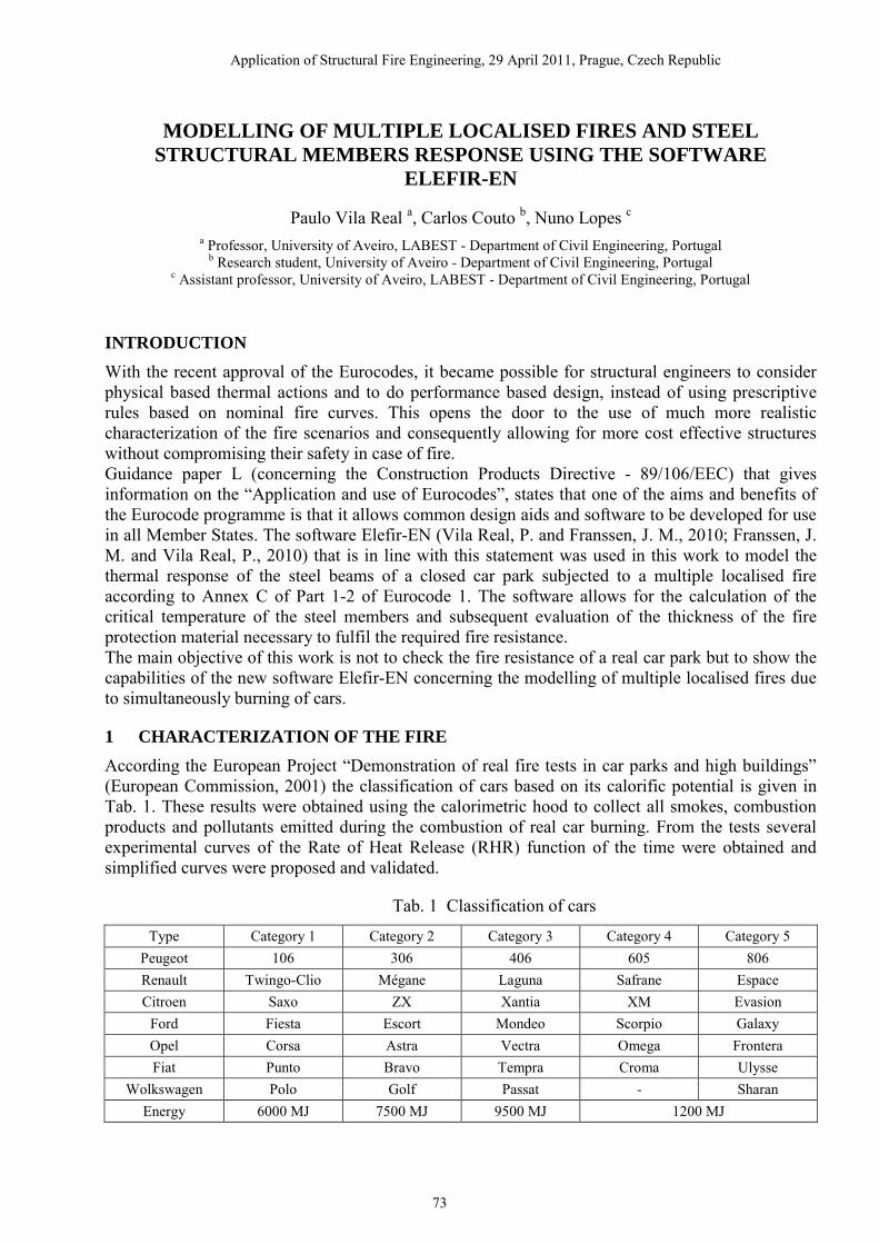
Application of Structural Fire Engineering, 29 April 2011, Prague, Czech Republic

MODELLING OF MULTIPLE LOCALISED FIRES AND STEEL STRUCTURAL MEMBERS RESPONSE USING THE SOFTWARE

ELEFIR-EN

Paulo Vila Real a, Carlos Couto b, Nuno Lopes c a Professor, University of Aveiro, LABEST - Department of Civil Engineering, Portugal

b Research student, University of Aveiro - Department of Civil Engineering, Portugal c Assistant professor, University of Aveiro, LABEST - Department of Civil Engineering, Portugal

INTRODUCTION

With the recent approval of the Eurocodes, it became possible for structural engineers to consider physical based thermal actions and to do performance based design, instead of using prescriptive rules based on nominal fire curves. This opens the door to the use of much more realistic characterization of the fire scenarios and consequently allowing for more cost effective structures without compromising their safety in case of fire. Guidance paper L (concerning the Construction Products Directive - 89/106/EEC) that gives information on the “Application and use of Eurocodes”, states that one of the aims and benefits of the Eurocode programme is that it allows common design aids and software to be developed for use in all Member States. The software Elefir-EN (Vila Real, P. and Franssen, J. M., 2010; Franssen, J. M. and Vila Real, P., 2010) that is in line with this statement was used in this work to model the thermal response of the steel beams of a closed car park subjected to a multiple localised fire according to Annex C of Part 1-2 of Eurocode 1. The software allows for the calculation of the critical temperature of the steel members and subsequent evaluation of the thickness of the fire protection material necessary to fulfil the required fire resistance. The main objective of this work is not to check the fire resistance of a real car park but to show the capabilities of the new software Elefir-EN concerning the modelling of multiple localised fires due to simultaneously burning of cars.

1 CHARACTERIZATION OF THE FIRE

According the European Project “Demonstration of real fire tests in car parks and high buildings” (European Commission, 2001) the classification of cars based on its calorific potential is given in Tab. 1. These results were obtained using the calorimetric hood to collect all smokes, combustion products and pollutants emitted during the combustion of real car burning. From the tests several experimental curves of the Rate of Heat Release (RHR) function of the time were obtained and simplified curves were proposed and validated.

Tab. 1 Classification of cars

Type Category 1 Category 2 Category 3 Category 4 Category 5 Peugeot 106 306 406 605 806 Renault Twingo-Clio Mégane Laguna Safrane Espace Citroen Saxo ZX Xantia XM Evasion

Ford Fiesta Escort Mondeo Scorpio Galaxy Opel Corsa Astra Vectra Omega Frontera Fiat Punto Bravo Tempra Croma Ulysse

Wolkswagen Polo Golf Passat - Sharan Energy 6000 MJ 7500 MJ 9500 MJ 1200 MJ

73

Fig. 1 shows the simplified RHR curve for a class 3 car fire. The referred project also suggests curves for the same type of cars that start burning with a delay of 12 and 24 minutes. In Fig. 2 these curves are shown and a fourth curve for of a car that starts to burn with a delay of 36 minutes has been added.

Fig. 1 Rate of heat release of a single class3 car fire

Fig. 2 Rate of heat release of a single class 3 car fire with a delay of 12 minutes

Tab. 2 gives the values of the rate of heat release as a function of time of each car with time delay of 12 minutes.

Tab. 2 Values of the rate of heat release of four burning class 3-cars

Time (min) 1st Car Time (min) 2nd Car Time (min) 3rd Car Time (min) 4th Car 0 0 12 0 24 0 36 0 4 1.4 13 2.4 25 2.4 37 2.4

16 1.4 22 2.4 34 2.4 46 2.4 24 5.5 28 5.5 40 5.5 52 5.5 25 8.3 29 8.3 41 8.3 53 8.3 27 4.5 31 4.5 43 4.5 55 4.5 38 1 42 1 54 1 66 1 70 0 74 0 86 0 98 0

1.1 Fire scenarios In this work, five fire scenarios, as shown in Fig. 3, have been considered according to the Rate of Heat Release of a class 3 car (see Tab. 1): i) Fire scenario 1: One car burning below the beam at mid-span; ii) Fire scenario 2: Three cars of class 3 in a normal parking bay with an ignition time delay for each car of 12 minutes; iii) Fire scenario 3: Four cars of class 3 in a normal parking bay with an ignition time delay for each car of 12 minutes It will be shown that the burning of the fourth car does not affect the maximum temperature of the beam; iv) Fire scenario 4: Three cars of class 3 in a normal parking bay with an ignition time delay for each car of 12 minutes; v) Fire scenario 5: Four cars of class 3 in a normal parking bay with an igntion time delay for each car of 12 minutes. In Fig.3 it is shown also the sequence of ignition of the different fire scenarios considered. The temperature of the beam was evaluated using the program Elefir-EN at the mid-span section and with the rate of heat release of the Fig.1 for Fire Scenario 1 and at the extremity of the beam and considering the rate of heat release of the Fig.2 in the remaining fire scenarios.

74

Fire Scenario 1

Fire Scenario 2 Fire Scenario 4

20 x 2.40 m

16.00 m

START

Fire Scenario 3

START

START

Fire Scenario 5

START

Fig. 3 Fire scenarios and sequence of ignition

1.2 Localised fires Annex C of part 1.2 of Eurocode 1 gives two models for the temperature development in case of a localised fire. Which one has to be used depends on the vertical length of the flame Lf given by the following Eq. (1):

5/20148.002.1 QDL f +−= [m] (1) where D is the diameter of the fire and Q the rate of heat release. Fig. 4, taken from Annex C of part 1.2 of Eurocode 1, shows the length of the flame when the fire source is on the floor level and the flame does not impact the ceiling.

Fig. 4 Localised fire not impacting the ceiling Fig. 5 Localised fire impacting the ceiling

When the flame does not impact the ceiling, Eurocode 1, based on the Heskestad method gives Eq. (2) for evaluating the temperature development )(tzθ that depends on the diameter of the fire D, the rate of heat release Q and the height z along the flame axis from the position of the source. 900)(25.020 3/5

03/2

)( ≤−+= −zzQczθ [ºC] (2) When the flame is impacting the ceiling ( HL f ≥ ; see Fig. 5) the Eurocode 1 based on the Hasemi

method, gives the heat flux h& [W/m2] received by the fire exposed unit surface area at the level of the ceiling (see Eq. (3)) as:

0.1if00015

0.130.0if00012130013630.0if000100

7.3 ≥=<<−=

≤=

− yyh

yyh

yh

&

&

&

[W/m2] (3)

This heat flux depends on the diameter of the fire D, the rate of heat release Q, the distance between the fire source and the ceiling H and the horizontal distance between the vertical axis of the fire and

75

the point along the ceiling where the flux is calculated, as shown in Fig. 5. According the Eurocode 1 this model can not be used in situation where the diameter of the fire source D is bigger than 10 meters and the rate of heat release of the fire Q is bigger than 50 MW. The method gives heat flux h& [W/m2] received by the fire exposed unit surface area and the net heat flux neth& , has to be calculated by

]293)273[(1067.5)20( 448 −+⋅×⋅⋅⋅Φ−−⋅−= −mmfmcnet hh θεεθα&&

[W/m2] (4) In case of several separate localised fires, Eq. (3) may be used in order to obtain the different individual heat fluxes 1h& , 2h& , 3h& . etc., received by the fire exposed unit surface area at the level of the ceiling. The total heat flux may be taken as: 000100...321 ≤+++= hhhhtot

&&&&

[W/m2] (5)

2 TEMPERATURE IN STEEL MEMBERS SUBJECTED TO LOCALISED FIRES

EN 1993-1-2 gives two different equations for calculating the temperature of steel members subjected to fire, depending on whether the members are protected or not. The procedures that are used to evaluate the temperature in the case of localised fires are presented in this section.

2.1 Unprotected steel members

EN 1993-1-2 provides a simple equation for calculating the thermal response of unprotected steel members. Assuming an equivalent uniform temperature distribution throughout the cross-section, the increase in temperature ta,θ∆ in an unprotected steel member during a time interval t∆ is given by:

thc

VAk dnet

aa

mshta ∆=∆ ,,

/&

ρθ [ºC] (6)

where the meaning of the variables can be found in the Eurocode. For unprotected sections, the heat flux used in Eq. (6) is the sum of a convective part and a radiative part, rnetcnetdnet hhh ,,,

&&& += . This heat flux is easily calculated if the gas temperature, gθ , is known. For localised fires not impinging the ceiling, the gas temperature is given by Eq. (2). In the case where the localised fire impinges on the ceiling, the heat flux is given by Eq. (3), and this can be directly used in Eq. (6) for calculating the temperature in unprotected steel members.

2.2 Protected steel members

EN 1993-1-2 provides a simple design method to evaluate the temperature development of steel members insulated with fire protection materials. Assuming uniform temperature distribution, the temperature increase ta,θ∆ of an insulated steel member during a time interval t∆ , is given by

( )( ) ( ) tg

tatg

aap

ppta et

cd

VA,

10/,,, 1

3/1/

θφ

θθρ

λθ φ ∆−−∆

+−

=∆ [ºC] (7)

the variables being defined in the Eurocode. This equation is only based on the gas temperature. For localised fires not impinging the ceiling, the gas temperature is given by Eq. (2) and the development of the steel temperature is calculated from Eq. (7). However, Eq. (7) can not be applied directly in the case of a fire impinging the ceiling, because the effect of the fire is given as an impinging flux, see Eq. (3). A procedure has to be established to transform the impinging heat flux into an equivalent gas temperature. Cadorin et al. (2003) suggests deducing a fictitious temperature that has the same effect on steel elements as the heat flux calculated with this method. This is the temperature of a steel profile with a very high massivity factor. This steel profile has a temperature which is very close to the gas temperature. This procedure is used in the program Elefir-EN. The program first evaluates the gas temperature as the temperature of a fictitious unprotected steel profile with very high section factor (Am/V = 10000 m-1 is adopted) using Eq. (6)

76

and the net heat flux given by Eq. (4). After evaluating the gas temperature, the temperature of the protected steel profile is then calculated using Eq. (7).

3 TEMPERATURES OF THE BEAM

The program Elefir-EN first evaluates the length of the flame to decide which method has to be used (Heskestad or Hasemi). In the case of multiple localised fires only the fires in which the flame impacts the ceiling are considered and the others are ignored. Fig. 6 shows the flame length development during the fire, considering that the diameter of the cars is D = 3.9 m and the height of the compartment is H = 2.7 m.

Fig. 6 Flame length development for a single burning car

Fig. 7 shows the gas temperature and the temperature of the main beam, supposing that it is made of IPE 500, the critical temperature is 540 ºC, the diameter of the cars is D = 3.9 m and the height of the compartment is H = 2.7 m.

a)

b)

c)

d)

77

e)

f)

Fig. 7 Temperature development. a) Scenario 1; b) Scenario 2; c) Scenario 3 d) Scenario 4; e) Scenario 5; f) Scenario 1 with the beam protected

Tab. 3 shows the maximum temperature obtained for the main beam in all the fire scenarios. From that table it can be concluded that, due to the scenario 1 the main beams should be protected so that the temperature doesn’t reach the assumed critical temperature of 540 ºC during the complete duration of the fire including the decay phase or during a required period of time. If the load-bearing function is required during the complete duration of the fire, the program Elefir-EN gives, for example, a need of 5 mm of sprayed vermiculite cement on the contour of the beam (see Fig. 7 f)).

Tab. 3 Maximum temperatures of the main beam

Scenario 1 Scenario 2 Scenario 3 Scenario 4 Scenario 5

max,aθ [ºC] 710.9 466.7 466.7 510.9 528.5

4 CONCLUSION

This paper has shown the capability of the software Elefir-EN for dealing with several separate localised fires. The software is an essential tool for structural engineers in the design office, enabling quick and accurate calculations to be produced, reducing design time and the probability of errors in the application of the equations.

REFERENCES

Cadorin, J.-F., Compartment Fire Models for Structural Engineering, Thèse de doctorat, University of Liege, Belgium, 2003.

CEN, EN 1991-1-2, Eurocode 1 – Actions on structures – Part 1-2: General actions – Actions on structures exposed to fire, Belgium, 2002.

CEN, EN 1993-1-2, Eurocode 3 – Design of steel structures – Part 1-2: General rules – Structural fire design, Belgium, 2005.

EUROPEAN COMMISSION, “Demonstration of real fire tests in car parks and high buildings”, Contract nº 7215 PP 025, 1 July 1998 to 20 June 2001.

EUROPEAN COMMISSION, Guidance paper L (concerning the Construction Products Directive - 89/106/EEC) - Application and use of Eurocodes, Brussels, 27 November 2007.

Franssen, J. M., Vila Real, P. – Fire Design of steel structures, ECCS ed and Ernst & Sohn ed., 2010.

Vila Real, P., Franssen, J. M. – Elefir-EN V1.2.3 (2010), Software for fire design of steel structural members according the Eurocode 3. http://elefiren.web.ua.pt.

78

Application of Structural Fire Engineering, 29 April 2011, Prague, Czech Republic

CONSTITUTIVE EQUATIONS FOR STRUCTURAL STEEL SUBJECTED TO FIRE

Some Remarks

Manfred Korzen a a BAM Federal Institute for Materials Research and Testing, Division 7.3 Fire Engineering, Berlin, Germany

INTRODUCTION

Although identified on the basis of so-called instationary creep-tests the constitutive model of Eurocode 3 (EN 1993-1-2, 2010) – hereinafter referred to as EC3 – represents a non-linear rate-independent relationship between stress and mechanical strain. I.e. the experimentally observed phenomenon of creep at constant stress but linear time varying temperature is described only through the temperature dependence of the material parameters characterizing the EC3 constitutive model. As a consequence some important phenomena cannot properly be described: E.g. creep or relaxation at constant temperature, creep or relaxation at non-monotonic temperature rates or sensitivity of the instationary creep process on the temperature rate.

1 CONSTITUTIVE EQUATION AND TESTING MACHINE AS AN OPERATOR

We attack our task to find a convenient constitutive equation for steel subjected to fire from the standpoint of the experimenter using a servocontrolled material testing system (s. Fig. 1), i.e. the material as well as the model is looked upon as an operator (Krempl, 1974). These operators map a time-dependent input (loading function) into a corresponding time-dependent output (response function). We limit our attention to uniaxial stress cases with macroscopically homogeneous states of stress and infinitesimal strain . According to this terminology a classical strain-controlled tension test at strain rate * and temperature * is defined by two loading functions: (i) *( )

and (ii) *( ) .const and one response function ( )t . We neglect any heating due to dissipation. The experimental input-output relationship, which is realized through the servo-controlled testing machine including the device for heating of the specimen, corresponds to a mathematical operator (Onat, 1972), i.e.

0

( ) ( ), ( )t

t

F . (1)

The symbol F defines an operator, which assigns with every ( ) and ( ) on [0, ]t a ( )t . It is a challenging task for the experimenter to identify the properties of this operator, which represents the material and is referred to as a constitutive equation. It is important to note that this equation is never obtained directly because in an experiment it is only possible to obtain a response function. Therefore, a constitutive equation must be constructed in such a way that it gives for a certain input the corresponding output like the tested material.

2 EC3 MODEL

The constitutive equation of EC3, i.e.

,mf (2)

defines a one-dimensional non-linear algebraic relation between , infinitesimal mechanical strain mech and temperature . It looks like a non-linear thermo-elastic constitutive model (s. Fig. 2) and

insofar as a special case of eq. (1). Therefore by definition eq. (2) is rate-independent, i.e. the

79

Fig. 1 Constitutive Equation and Material as an Operator (figure below after Morrow, 1965) Fig. 2 Non-Linear Elastic Behavior

material response does not depend on the rate of loading. Another point of view is achieved through the well known fact, that the experimental basis of eq. (2) are so-called instationary creep tests. Those type of tests are characterized through loading functions L and L of type

*( ) .L const , (3) *( )L . (4)

I.e. the specimen is loaded up to * and then at this stress level heated up with a temperature rate of * . The response functions for N tests at N stress levels look like

* *1 1 1( ) ., ( )t g const t t (5.1)

* *( ) ., ( )N N Nt g const t t . (5.N)

Each response function depends on the stress level and on the temperature rate. We achieve at eq. (2) assuming that * and * are no longer parameters but variables and inverting eq. (5) to give

,f (6)

and after subtracting the thermal strain

,mf . (2)

I.e. the stress-strain relationship of EC3 is derived through the usage of response functions as constitutive equations. Keeping that in mind a more precise characterization of eq. (1) would be that it gives the necessary constant stresses to reach a given mechanical strain mech at a heating rate of

* . Especially, the phenomenon of creep at constant temperature and the influence of the temperature rate on creep cannot be described through eq. (2).

3 CONCEPT OF A CONSTITUTIVE MODEL

Due to the shortcomings of the EC3 stress-strain relationship we are looking for a more appropriate constitutive equation especially with concern to the experimental phenomenon of classical as well as instationary creep. Our model is based on the very classical three-parameter solid of viscoelasticity (Flügge, 1975). Only two main modifications are introduced: (i) the strain is replaced by the mechanical strain mech and (ii) the static stress stat , i.e. the stress response for

80

slow motions, is no longer a linear function – as in linear viscoelasticity – but a rate-independent functional of the deformation variable so that we have finally

0

1, 0 0

,stat mech

statE

(7)

, ( ), , , 0 0stat mech m stat mech statg sign (8)

with

( ) ( ) ( ) ( )

. : ( )( ) ( ) ( ) ( ) ( )

mech stat meche p

e mech stat meche p

E sign Eg E

E sign E

(9)

0: ( )mech (10)

where () denotes the material time derivative. Round brackets are symbols for “function of” whereas square brackets are used in the algebraic sense. Eqs. (7) and (8) (s. Fig. 3) define a system of non-linear non-autonomous ordinary differential equations of type

0( ), , (0)y h y t t y y (11)

with initial conditions for and stat . Eq. (11) may be stiff in certain regions (Hairer et al., 2002). Eq. (8) (s. Fig. 4) defines implicitly the aforementioned rate-independent functional for the static stress stat (Valanis, 1980). In contrast to classical constitutive equations of elasto-plasticity eq. (8) is defined without a yield surface and corresponding loading conditions. Eqs. (7) and (8) belong to the class of so-called unified theories which do not separate plastic and creep strains, and represent inelastic deformation by a set of equations, employing a number of internal variables. In our case one internal variable is used and corresponds to stat .

Fig. 3 Spring-dashpot model of proposed constitutive equation

Fig. 4 Stress-strain diagram of static stress with temperature dependent material parameters

In the asymptotic limiting case of fast loadings ( , mech ) eq. (7) reduces to

0mechE , (12)

i.e. a linear elastic response with the temperature dependent spontaneous Young’s modulus 0E .

The limiting case of slow loadings ( 0 , 0mech ) yields stat , (13)

i.e. a hysteretic response (s. Fig. 4) , which is represented by the static stress stat . Beside this qualitative analysis numerical simulations are realized with the software package RAUDAU (Hairer, 1996).

81

4 STRESS AND TEMPERATURE CONTROLLED INPUT FUNCTOIN - CREEP

In order to simulate creep, i.e. to define stress and temperature as input functions in the terminology of chapter 2, we have to arrange the constitutive equations in the following form:

00

, 0 0,

statmech mech

stat EE

(14)

, ( ), , , 0 0stat mech m stat mech statg sign (15)

Assuming that the material parameters relaxation time , spontaneous Young’s modulus 0E as well

as the parameters , , eE and pE of the static stress are identified as functions of temperature we

can use the constitutive model as an operator to run simulations for different inputs of stress and temperature. As an example we run some simulations for the case of instationary creep. The material responses in Fig. 5 demonstrate the sensitivity of the creep response to temperature rate. In Fig. 6 it can be observed what happens if the temperature switches from one value to the other in comparison with the corresponding behaviour at constant temperature rate. The simulated material responses represented in both figures looks plausible but are in contrast to the EC3 model behaviour which does not show any sensitivity to temperature rate.

Fig. 5 ( )mech t at * = 100 MPa and different *Fig. 6 ( )mech t at * = 100 MPa and different *

with jumps in *

5 COMPARISON BETWEEN MODEL AND EXPERIMENT

In order to make a quantitative comparison between the proposed model and experiment we executed a special transient creep test with a specimen of S235 steel. In contrast to the classical heating with a ramp of constant temperature rate we realized it with a triangle temperature-time pattern. The heating was realized through high-frequency inductive coils, which normally are used for so-called TMF (thermo-mechanical fatigue) tests. The strain was measured with a special clip-on extensometer directly attached to the surface of the specimen. The experimental results as well as the data of the numerical simulation are presented in Fig. 7. The bottom figure demonstrates the extraordinary precise realization of the temperature input function together with the input function for the simulation. The top figure visualizes the measured total strain ( ) together with the simulated thermal strain (top), total strain (middle) and mechanical strain (bottom). The correlation between model and experiment is quite good.

82

Fig. 7 Input (temperature) and output (strain) of non-monotonic transient creep test at * = 100 MPa and *| | = 7 K/min, : experimental data

6 SUMMARY AND ACKNOWLEDGEMENT

After introducing the operator point of view on material and constitutive equation the EC3 model has been discussed together with its shortcomings. An alternative constitutive equation approach within the operator terminology was presented together with its basic capabilities. Finally the behaviour of the proposed model was compared with the results of a challenging experiment related to transient creep, and demonstrated a quite good correlation. The author is very grateful to Le Trung Nguyen who has done all simulations.

REFERENCES

EN 1993-1-2, Eurocode 3: Design of steel structures – Part 1.2: General rules- fire design, CEN (Comité Européen de Normalisation), Brussels, Belgium, 2010)

Flügge W., Viscoelasticity, Berlin, 1975.

Hairer E. Wanner G., Solving ordinary differential equations II, Berlin, 2002.

Hairer, E., RADAU5, Université de Genève, 1996.

Krempl, E., Cyclic Creep – An Interpretative Literature Survey, Welding Research Council Bulletin, No. 175, 1974, 63-123.

Morrow J., Cyclic plastic strain energy and fatigue of metals, ASTM STP No. 378, 1965, 45-87.

Onat E.T., Fardshisheh F.; Representation of creep of metals, Oak Ridge National Laboratory, Oak Ridge, Tennessee, U.S.A., Report ORNL-4783, 1972.

Valanis K.C., Fundamental consequences of a new intrinsic time measure. Plasticity as a limit of the endochronic theory, Archives of Mechanics 32 (1980) 171-191.

83