Pragmatic Guide for Using the FUNCube (AO-73) Materials Science Experiment in

the Classroom

February 2014

Mark Spencer, WA8SME ARRL Education and Technology Program mspencer@arrl.org 860-381-5335

TABLE OF CONTENTS Installment Title Page 1. FUNCube MSE overview and thermodynamics refresher 1 2. Accessing the FUNCube over-the-air and over-the-web 9 3. An affordable Leslie’s Cube Experiment system (that you can build) 19 for demonstrating the thermodynamics of the MSE 4. A simple MSE In-classroom Simulator (that you can duplicate) 26 that mimics the data being collected on the satellite 5. Interpreting real FUNCube MSE data being collected on the satellite 31 6. Further studies using MSE data 45

1

1. FUNCube MSE overview and thermodynamics refresher Introduction. This collection of activities is intended to be an instructional guide to help teachers and ham radio satellite enthusiasts to access and use the AMSAT-UK FUNCube Materials Science Experiment (MSE) resource carried on-board AO-73 in their classrooms, local schools or in their ham shacks. The Guide makes a ‘how-to’ pamphlet to include the following chapters:

FUNCube MSE overview and thermodynamics refresher (this installment) Accessing the FUNCube over-the-air and over-the-web An affordable Leslie’s Cube Experiment system (that you can build) for demonstrating

the thermodynamics of the MSE [The Leslie’ Cube Experiment is used to measure or demonstrate variations in energy radiating from different surfaces.]

A simple MSE In‐classroom Simulator (that you can duplicate) that mimics the data being collected on the satellite 

Interpreting real FUNCube MSE data being collected on the satellite Further studies using MSE data

FUNCube MSE Overview. The primary mission of the FUNCube is education. The secondary mission is a transponder for use by ham radio operators to use to communicate via satellite. The FUNCube has been awarded the OSCAR designation AO-73, therefore throughout the Guide FUNCube and AO-73 will be used interchangeably. The most up to date status and specifics of AO-73 can be found at the AMSAT-UK web site dedicated to the satellite at: http://funcube.org.uk/. The focus here of course is on the education mission. Purpose of the Materials Science Experiment (MSE) as quoted from The AMSAT-UK FUNCube Handbook is: “…This examines how heat energy is radiated into space from materials with different surface finishes. In the school science lab we learn that heat energy transfers from a hot material to a cold material by conduction convection or radiation. While conduction in solids and convection in gasses or liquids can be easily demonstrated, the classic Leslie’s cube demonstration to show energy transfer by radiation can be unconvincing, as conduction and convection occur at the same time. Funcube-1 has two aluminum bars mounted on the external surface of the solar panels. One sample is anodized matt black, the other has a highly polished Chrome finish. Both 70 x 4 x 3mm samples [bars] are thermally isolated and include thermistors to measure their temperature. As the satellite passes through the illuminated part of its orbit, energy from the sun is absorbed into both metal samples causing an increase in temperature. The difference in temperature rise between the two samples is not easily predicted as it depends not only on the known attributes of mass, surface finish, specific heat capacity and surface area but also on several unknown variables - for example satellite rotational rate, attitude and the angle of the sample to the Sun. However, when the satellite passes from sunlight into eclipse, energy is lost from both samples by radiation.

2

Figure 1.

AMSAT-UK Photo

The temperatures are sampled once every 60 seconds and stored in the satellite[‘]s memory. As FUNcube passes over a ground station, data for the last 104 minutes is transmitted via the telemetry. As the time taken for one orbit is approximately 94 minutes, the data will include the last pass through eclipse. The data can be plotted as a graph using the ‘dashboard’ software. It shows how energy is absorbed and emitted from the samples by radiation at different rates. In addition to the MSE samples on the solar panels, the aluminum vertical corner struts of the satellite have been produced with one side having a natural silver finish (covered with a blue kapton coating before launch) while the others are matt black. All of these surfaces can be seen on the cover photograph, the formal samples are mounted above the right-hand solar panel. Temperature sensors have also been included and although the structure is screwed together allowing the conduction of heat energy from the corner struts, there should be a measurable difference in the rate of temperature change between them all…” The FUNCube MSE hardware described is configured as illustrated in the picture of the satellite in Figure 1.

As stated, there are actually two different experiments included in the MSE, one using the thermally isolated aluminum bars mounted on one of the satellite faces, the other using four aluminum bars mounted as part of the satellite body in the corners of the cube. These corner bars are not thermally isolated from the rest of the satellite superstructure.

3

Figure 2.

The data collected by the MSE is transmitted via a VHF data link on frequency 145.935 MHz (with appropriate Doppler corrections) using Binary Phase-Shift Keying (BPSK) and can be received with common ham radio equipment capable of receiving Upper Side Band (USB) signals. AMSAT-UK has published a free and downloadable companion software package called the Dashboard that includes a soundcard based interface that translates the BPSK audio fed into the computer sound card into decoded telemetry values and graphics that are displayed in real time or that can be recorded, saved, and retrieved from a central database for later analysis. The specifics of how to set up a basic station to receive MSE data will be covered in the next section. However, here I will just illustrate the kind of output you can expect from a typical FUNCube pass to whet your appetite.

Figure 2 illustrates the graph of the typical Whole Orbit Data (WOD) MSE temperature profiles of the anodized black and chrome, thermally isolated bars mounted on the face of the satellite. The graph begins as the satellite emerges from the eclipse portion of the orbit (when the satellite is in the Earth’s shadow and not illuminated by the Sun). The temperatures of the bars rise as they receive heat energy from the Sun. About mid way through the graph (orbit), when the temperatures start to drop, the satellite is entering the next eclipse phase of the orbit and the bars give up heat to the surrounding space. The graph indicates a lot of intriguing things going on during the orbit, some are expected and predictable, others are very much a surprise and counter intuitive…all however make the FUNCube MSE an exceptional learning experience for students (and ham radio operators too). It is fun and technically challenging to receive the MSE data, but the real in-depth learning comes from interpreting the data as presented in the graphs. To begin to interpret the graphs, a short refresher of basic thermodynamics is in order. Thermodynamics Refresher. The following is going to be an over-simplified review of basic thermodynamics. I know I am taking some liberties to short cut the topic for the sake of brevity and in an attempt to reach an audience of broad interests, backgrounds, and proclivities. I am by

4

no means an expert in thermodynamics. So with that caveat in mind, let’s review thermodynamics…a very hot topic. In the broadest terms, thermodynamics is the study of how heat moves from one place to another. Heat transfer is fundamental to our very existence…our lives depend on the heat energy that comes from the Sun. How that heat gets here to Earth, and how we deal with it once it is here, is thermodynamics…and the focus of the FUNCube MSE. All matter or material contains some amount of heat energy, and heat energy conforms to three basic laws of thermodynamics: First Law of Thermodynamics. The first law of thermodynamics deals with conservation of energy. Heat is a form of energy that manifests itself within a material as an increase in the kinetic energy of the individual atoms or molecules that make up the matter. The increase in heat energy content is indicated as an increase in the temperature of the material. Second Law of Thermodynamics. Heat energy naturally moves from a higher temperature source to a lower temperature sink of heat. An example of this process would be the heating elements of your kitchen stove top and a frying pan. Heat energy can also flow from a lower temperature source to a higher temperature sink if work is applied to the system to force this reverse flow. An example of this process would be your kitchen refrigerator which uses work performed by the refrigerator compressor and cooling coil unit to move heat from the relatively cold refrigerator interior to the relatively warm exterior room. The second law of thermodynamics is the focus of the FUNCube MSE. Third Law of Thermodynamics. The third law simply states that at a temperature of absolute zero degrees Kelvin (0 K is approximately -273.15 degrees C), molecular kinetic activity stops and therefore there is no heat energy. It is considered physically impossible to achieve absolute zero but we can get very, very close (the effective temperature of outer space is approximately 3.5 degrees K or -269.6 C). The utility of the third law is that absolute zero becomes a reference point. The amount of heat energy a material contains is relative to the temperature of absolute zero degrees. There are three ways that heat energy moves from point A (the higher temperature) to point B (the lower temperature); convection, conduction, and radiation. Heat transfer by convection and conduction require a medium in contact with the heat source through which the heat energy moves. Conduction is heat transfer by means of molecular agitation within a material without any motion of the material as a whole. In conduction, the vibrating atoms or molecules run into adjacent atoms or molecules imparting some kinetic energy to those adjacent atoms or molecules causing them to vibrate… in turn resulting in the heat energy traveling by this “contact” between adjacent particles from the high temperature side toward the low temperature side (much like colliding billiard balls). The heat will continue to move until the overall temperature gradient is equalized (then the heat energy moves back and forth throughout the material randomly).

5

Convection is heat transfer by the motion of a fluid such as air or water when the heated fluid is caused to move away from the source of heat, carrying energy with it. In convection, the medium is a fluid (either gas or liquid) in contact with the higher temperature source. The atoms or molecules within the higher temperature source impart heat energy to the fluid atoms or molecules in contact with the material surface. This heating adds kinetic energy to the fluid and causes the fluid to expand (become less dense), resulting in the higher temperature fluid rising and moving away from the heat source material taking heat energy with it. In radiation, heat energy behaves as an electromagnetic wave (like light or radio waves) allowing it to move without a medium from the high temperature source to the low temperature sink. Heat radiation emitted by a body is a consequence of the thermal agitation of its composing molecules and atoms. The heat movement by radiation will continue in one direction until the difference in temperature becomes zero and the heat energy then flows back and forth randomly in either direction with the overall average movements being equal (no net energy transfer). On Earth, heat transfer by conduction and convection are major contributors to the movement of heat. In the near vacuum of space, heat transfer away from a space craft cannot occur by convection because there is no fluid medium available. The lack of a medium makes space an ideal location to study radiation, but also makes controlling heat in a spacecraft a more difficult challenge than on Earth. This makes the FUNCube MSE an attractive (and also important) experiment to study heat transfer by radiation. By the numbers. There are a couple of mathematical formulas that we can use to show the relationship between heat transfer and the other factors that influence the way heat energy is transferred from a higher temperature source to the lower temperature sink (i.e., the second law). The first equation expresses the heat content of a material relative to absolute zero, and can be used to calculate the amount of energy required to change the temperature of the material.

∆ equation 1. Where: Q = heat energy in Joules; m = the mass of the material or object in grams; cp = the specific heat property of the material; and ΔT is the difference in temperature (if T1 = absolute zero, then the quantity of heat is relative to zero heat energy). For the aluminum used in the bars of the MSE; cp = .9Joules/(gram*degrees Kelvin); the mass of the bars is 2.4 grams each. The second formula of interest is:

equation 2. This the Stefan-Boltzman Law which governs the net radiation from objects where: P (power) = ΔQ/Δt = Joules/time in seconds = W (watts); e is emissivity (0 < e <1); σ is the Stefan-Boltzman Constant (5.67 X 10-8 W/(m2*K4); A is the exposed surface area of the bars (7.24 X 10-5 m2); and T1 and T2 are in degrees Kelvin. An electronics analogy for equation 1 would be an RC circuit where Q would equate to the charge accumulated in the capacitor over time, the mass and specific heat property of the

6

material would equate to the value of capacitance, and the temperature difference would be the applied voltage charging the capacitor. If the voltage of the source is greater than the voltage across the capacitor, the capacitor accumulates charge, if the voltage of the source is less than the voltage across the capacitor, the capacitor will discharge. An electronics analogy for equation 2 would be Ohm’s Law where the change in heat content over time would equate to current flow, the inverse of emissivity and the Stefan-Boltzman constant and surface area terms would equate to resistance, and the temperature difference would equate to the voltage. In other words, the greater the temperature difference (voltage magnitude and polarity) the greater the driving force causing heat energy to move (current magnitude and direction) through some restrictive property (emissivity and surface area). Let’s take a closer look at one of these restrictive properties, emissivity. Emissivity is a physical property of a material that represents the ability for heat energy to radiate (leave) the material. Emissivity is relative to the material’s ability to radiate heat energy in comparison to a perfect radiator, the “black body”, and is expressed as a unit-less value between 0 and 1. The emissivity of a black body is 1. In other words, emissivity of a material is a ratio or percent of the heat energy it radiates in comparison to the heat a black body would radiate at a temperature. A black body is an object that absorbs 100% of the radiant energy that strikes it, and if in equilibrium with the surroundings, it emits all of its energy also. Returning to the electronics analogy, emissivity would be conductivity (the reciprocal of resistance). The relatively simple concept of emissivity can very quickly become a very complex topic. The emissivity of a material depends on the wavelength of the heat energy being transferred, temperature of the material and the uniformity of the temperature distribution, body geometry, and surface texture of the body (reflectivity). To deal with this complexity, some assumptions and simplification is in order. Consequently, engineering tables of physical properties will generally list a material’s total emissivity as the physical property. Total emissivity is defined as the resulting value when the individual emissivity factors (from wavelength, temperature, etc.) are averaged over the total radiation spectrum being utilized. The emissivity of black anodized aluminum is 0.77, the emissivity chrome plated aluminum is 0.056. Every material radiates energy. The amount of heat energy radiated is dependent on the material’s temperature, the temperature of the surroundings, and the emissivity. So after all that, what does that mean? If we were to take two identical aluminum bars (mass and geometry), one with a black anodized coating and the other chrome plated, both at the same starting temperature, and expose them to the same source of heat (such as a heat lamp), a plot of the bar temperatures over time would be as illustrated in figure 3. There is no physical contact between the light source and the aluminum bars so there is limited conduction. In this example, the light source is located above the aluminum bars so there is limited convection (the heated air from the light bulb rises away from the aluminum bars)…leaving radiation as the predominant transfer mechanism. While interpreting the graph, refer to equation 2.

7

Figure 3.

[This figure 3 will be referenced frequently thought the rest of the Guide, you might consider flagging this page to facilitate returning to the figure later.] The black line is the black panel temperature, the gray line is the chrome panel temperature. As the bars are exposed to a steady illumination, both bars accumulate heat energy by radiation but because the black bar has a higher absorptivity, it more efficiently absorbs heat when compared to the chrome bar that has a lower absorptivity. (By definition in our simplified presentation in the thermodynamics review, emissivity equals absorptivity for black bodies.) In this example, at the end of the illumination time period, the temperature difference between the black bar and the chrome bar is approximately 55 degrees C. Conversely, when the illumination is removed (the light is turned off), the bars lose heat energy to the surroundings. The black bar loses energy at a higher rate than the chrome bar because the emissivity of the black bar is greater. At the end of the elapsed time, the two bars are virtually at the same temperature. (The graphic was produced using a simple bench top experiment that will be detailed in chapter 4 of the Guide.) Summary of the thermodynamic review. So after this lengthy discussion, what is the bottom line? The amount of heat energy that is absorbed by, or radiated from, a material depends on material’s temperature, the temperature of the surroundings, and the emissivity of the material. The purpose of the FUNCube MSE is to allow students to witness heat transfer by radiation first hand in an environment (space) where convection and conduction are not present. I hope by now, if you didn’t see it right off the bat in figure 2, you see the elephant in the room; why are the temperature plots of the FUNCube MSE data so different than the theoretical plots in figure 3? The disconnect between what I expected to see from the MSE data (something similar to figure 3), what I just described in the fundamentals of thermodynamics, and what I actually was seeing, hit me between the eyes the very first time I plotted the MSE data. That disconnect

8

from the very first orbit of FUNCube started me on the quest that brought me to this point. You’ll have to wait and see the outcome of my struggle to understand and try to explain the disconnect (to be covered in the future installment on interpreting real FUNCube MSE data). The next installment of the Guide will provide some recommendations of the minimum satellite ground station equipment needed to directly receive the usable FUNCube MSE telemetry from the satellite in orbit.

9

2. Accessing the FUNCube over-the-air and over-the-web Introduction. In this installment I will discuss just one of many approaches that can be used to receive FUNCube telemetry for analysis in the classroom. My goal here is to provide a starting point for setting up minimum satellite ground station equipment to achieve some level of success. Also, accessing the archived telemetry that was received by other stations around the globe, as well as accessing whole-orbit-data (WOD) that was collected and stored on-board the satellite and later uploaded to an internet based data base will be briefly presented. What do you need? To receive telemetry from AO-73 you will need at a minimum:

The FUNCube Dashboard software running on a computer, with a sound card and running the appropriate operating system .

A two meter radio capable of receiving Upper Side Band (USB) with a variable frequency oscillator (VFO) resolution of around 20 Hz.

Interconnecting cabling between the receiver audio output and the computer sound card and feed line cabling between the receiver and the antenna.

An antenna designed for the two meter band. To access the data that is stored in the archives maintained on the world-wide-web, you will need an internet connected computer with graphing capable software installed such as Excel ®. Dashboard. The AMSAT-UK Dashboard software is an all in one telemetry decoding and display software package that is available from the http://funcube.org.uk/ web site. Simply visit the FUNCube web page (where there is a wealth of FUNCube satellite related information), download the software and follow the installation instructions. The software is very intuitive to operate and easy to get up and running. Along with displaying the telemetry data received from the satellite in real time (numerical values for all the different satellite housekeeping variables being monitored), there are tabs for displaying the MSE data in graphic form. Included in the software package is a sound card interface that accepts the audio from the receiver (more about the receiver in the minute), automatically tunes the sound card to correctly decode the imbedded binary stream in the audio, and decodes the binary stream for use in other parts of the software. A few examples of how to use this tuning feature with a traditional (non-FUNCube Dongle) receiver will follow shortly. Receiver. AMSAT-UK has developed a thumb drive, software defined radio (SDR) receiver called the FUNCube Dongle. There is extensive information on the Dongle, how to obtain one, how to install the requisite software, and how to use the Dashboard to control this receiver located on the FUNCube web page and I will not try to duplicate that exceptional information here. I will focus on how to use a traditional two meter, all-mode receiver with the Dashboard. The AO-73 telemetry is transmitted on a frequency of 145.935 MHz using BPSK modulation. A standard 2-meter hand-held FM transceiver will not work to receive BPSK so you will have to use a multi-mode receiver. Many common all-band, HF transceivers on the market (and probably in your shack) include the 2-meter band and these receivers will work fine to receive

10

Figure 1.

FUNCube BPSK using USB mode. Additionally, the VFO should have a frequency resolution on the order of 20 Hz or better. You simply have to construct an audio patch cable between the receiver audio output jack and the microphone input jack of your computer sound card. I have found it useful to use an isolation transformer circuit between the receiver audio and the computer microphone line to improve the interconnection. There are many commercially available radio interfaces, but you can easily construct one. Figure 1 is a simple circuit as an example.

I personally have used these 2-meter capable receivers around my shack with good success to receive AO-73 telemetry: IC-910 (my main satellite transceiver), IC706, IC746Pro, FT-817 (used for the antenna tests detailed below), and a Yaesu R5000 receiver. Using the Dashboard with one of these receivers will be discussed in a moment. Antenna. There are as many opinions as to the most appropriate or effective antenna to use in your ground station as there are individuals setting up ground stations. Additionally, there is the complication of defining what “effective” means. In the following discussion, I define an effective FUNCube antenna is one that allows the users to receive and decode sufficient telemetry frames to display meaningful graphs that can be used to interpret what is happening with the satellite…and even this definition is up for interpretation. The spectrum of “sufficient” goes from one extreme of correctly decoding every frame that is transmitted by the satellite while it is in your footprint (over your local horizon) to the other extreme of simply being able to hear the telemetry being transmitted, but not necessarily decoded correctly. The upper extreme is virtually impossible to achieve, the other extreme maybe a good starting goal, but of minimal education value. You also need to consider the cost and complexity of the antenna and any installation restrictions. So the most appropriate antenna is a complicated question to answer. The VHF telemetry signals from AO-73 are relatively strong and fairly easy to hear with simple antennas. The telemetry will sound like an increase in noise level, with a simultaneous dual-tone “beep” being transmitted every five seconds. Once you hear AO-73 you will be able to distinguish between receiver background noise and the noise of the BPSK signal (as well as be able to see the difference on the Dashboard display). But being able to hear the telemetry signal is not the same as having sufficient signal quality to decode the signal. Intuitively, the better the

11

signal quality and strength, the more telemetry frames that will be properly decoded. Generally better signal quality means larger, directional, and more expensive antenna systems that are pointed to track the satellite in orbit. But you don’t need 100% decoding to receive very good telemetry plots for AO-73. What is the minimum signal quality needed to decode the number of frames of telemetry data to be useful in the classroom? The criteria that I set for my analysis is that there should be sufficient number of frames decoded so that the student can use the high resolution plots of the Sun sensor data to determine the rotation rate of the satellite. Additionally, there should be a sufficient number of frames decoded so that the plots of the whole orbit data (WOD) do not have significant gaps that detract from the integrity of the plots. Granted, these criteria are very subjective. But the bottom line is that you will need to decode a minimum of approximately 50 frames. (Frame count is reported by the Dashboard software.) Here are a few details about the telemetry protocol. There are 24 frames of data sent, one frame every 5 seconds, or a complete data set transmitted every 2 minutes. The telemetry data set includes:

RT (real time data) and WOD contained in 12 frames (WO1 – WO12) RT and Fitter Messages in 9 frames (FM1 – FM9) RT and High Resolution in 3 frames (HR1 – HR3) For a total of 24 frames

Ideally, all you need to receive is a complete data set of 24 frames during a pass, and technically this is the minimum number of frames you would need to receive…if each of the 24 frames is decoded correctly when it is first received. This is very possible, but not always likely. Therefore you will need to collect as many frames as you can so that if there are lost frames, at some point during the pass through your footprint, there is a good potential that subsequent frames will “fill in the gaps” to complete the data set. If however, you fail to collect the missing frames, the data is lost and the graphs will be incomplete and perhaps corrupted. The following graphics illustrate what I mean. Figure 2 shows the plots of WOD for the Black Panel of the MSE for an antenna that produced 50 decoded frames at the top, and another antenna that produced 61 decoded frames at the bottom.

12

Figure 2.

As you can see, the loss of data with only 50 decoded frames is insignificant. There must have been one lost WOD frame in the first plot. In all likelihood, any lost WOD frames in the second plot were subsequently “filled in” to complete the data set. The capture of the high resolution data is a different matter. The high resolution graph information is transmitted in an interrupted format, one minute of data collected at 1 second intervals, one minute pause with no data collected, then repeat. Figure 3 illustrates an apparent complete high resolution data set from a pass that resulted in over 90 collected frames. Note the close data dots during the 1 minute collection window, and the lines (without dots) during the 1 minute pause interval. Because of this toggling between collection and pause, you need sufficient data to extract information from the graph.

13

Figure 3.

Figure 4.

It would be easy to determine the rotation rate of the satellite based on this data. (The period between the falling edges of illumination during each rotation.) Alternatively, figure 4 shows the high resolution graphic of the Sun Illumination sensor from the 50 decoded frame pass.

While defining beginning of the illumination of the panel surface is obvious in the middle of the graph, the loss of data early in the graph shows that the other beginning illumination point is missing, making the begin illumination point questionable. You could not determine the satellite rotation rate from this data. Figure 5 shows the high resolution graphic of a 61 decoded frame pass.

14

Figure 5.

The end of illumination points are easily identified in this graphic and the rotation rate of the satellite can be determined by comparing the times at these points. Interestingly, if you apply the Nyquist principles to the collection of the frames, a rough approximation is that 48 frames would be needed. This seemed to be verified with my unqualified suggestion that 50 decoded frames are needed to gather usable data (unless you are lucky to catch the right frames and the right time). Getting back to the antenna recommendation, I did a somewhat qualitative comparison of the antennas at my disposal to determine which would likely produce 50 decoded frames:

My primary satellite antenna system, the M^2 2MCP14 RH Circular Polarized Yagi with antenna mounted preamps and hard line coax.

An ARROW antenna with Preamp and rotator. An ARROW antenna fixed pointing straight up with and without a preamp. A simple 2-meter turn-style antenna (RHCP) with and without a preamp. A 5/8ths wave vertical whip antenna with and without a preamp. A ¼ths wave vertical ground plane antenna with and without a preamp.

I used the primary antenna as the base line antenna to obtain about as many decoded frames as can be expected with an (arguably) top of the line but affordable antenna system. The other antennas were used with and without an antenna mounted preamp and in different configurations. The preamp was an inexpensive broadband, battery operated circuit of unspecified gain (it is cheap but it works). The coax run between the receiver and the antenna was 80 feet of RG8 Mini coax. I collected telemetry data from AO-73 orbits that were of similar elevation (the elevations were at 35 degrees +/- 15 degrees) so the comparisons are not going to be exact by any means. I simply plotted the number of correctly decoded telemetry frames against the antenna configuration. The results are depicted in figure 6 (R = rotator, P = preamp, Up = pointed straight up).

15

Figure 6.

My recommendation based on this evaluation is that an antenna mounted preamp is most important to mitigate the signal loss from the coax run between the radio and the antenna. Second, just about any fixed installation, single element antenna will work (vertical antennas)…though I did not test it, I expect that radio mounted antennas (like a rubber duck antenna) will not give satisfactory results. Third, I would recommend that some sort of directional antenna that is rotator controlled to keep the antenna tracking the satellite should be a goal, eventually you will want to use other satellites and will want or need the added gain that these kinds of antennas provide. Accessing whole orbit data from the FUNCube archive. You will find a link on the FUNCube web page to the database of WOD and the High Resolution data. These files contain comma delimited data sets that you can import into Excel and in turn use the graphing capabilities of Excel to graph the data (a wod.csv file extension that brings you right to Excel and a loaded spreadsheet). You may have to adjust some of the fields at the beginning of the file to get the columns to match up correctly. The main column headings that were of interest were these:

Satellite Date/Time UTC 

Black Chassis deg. C 

Silver Chassis deg. C 

Black Panel deg. C 

Silver Panel deg. C 

Operating the Dashboard with a non-FUNCube Dongle receiver. One of the teachable moments in using the FUNCube in the classroom is the fact that the downlink frequency will experience Doppler shift during its transit through your area. The Dashboard sound card interface will track

16

Figure 7.

some of this Doppler shift within the audio pass band of the traditional receiver, but generally you will find that the Doppler shift for FUNCube will be approximately +/- 3KHz, which will require some tuning of the receiver VFO during the pass to facilitate the maximum decoding of transmitted telemetry frames. You can use a satellite tracking and radio station control program such as SatPC32 to automatically correct for Doppler shift, or you can watch the Dashboard tuning display and make minor frequency adjustments during the pass to keep up with the Doppler shift manually when the shift approaches the edges of the receiver pass band. Once you have your receiver connected to the computer sound card, launch Dashboard and you will see the blank spectrum display at the bottom of the window. Click on Capture then Capture From Soundcard in the menu bar. When you turn on your receiver, tune to 145.935 +Doppler, and you will see the spectrum display between 0 and 4,000 Hz of the USB audio pass band of the receiver (figure 7).

With the Auto Tune box checked, the Dashboard will track to the “peak” in the pass band. When the BPSK signal rises above the noise level (you will hear the background noise change from receiver noise to the BPSK noise), the software will lock on and track the BPSK and start decoding the frames. Every 5 seconds the satellite will transmit two tones simultaneously that brackets the BPSK signal. These tones show up as “horns” that help to keep the signal in tune (figure 8).

17

Figure 8.

If you are using a satellite tracking program to correct for Doppler, you should be able to let the system run and Dashboard will compensate for any minor changes needed in frequency due to Doppler tracking imperfections. If you are manually tracking Doppler, with practice you will notice that the “horns” are approaching the upper limit of the pass band peak indicating a minor downward correction of the receive frequency (using the VFO dial) is in order. Make the adjustments and Dashboard will do the fine tuning for you. As the data is decoded, the Dashboard Real Time Display will be updated with the current information (figure 9).

18

Figure 9.

At the end of the pass, the graphs generated by the Dashboard can be viewed by clicking on the appropriate tabs. Your collection session can be saved locally to a file on your computer by clicking on File and Save Session As… You can also set up an account to upload your collected data to the central data base by configuring the Dashboard appropriately as detailed in the help files (File and Settings…). Summary. After a little operating practice you will be collecting quality telemetry data from the satellite. Then the real learning begins when you start interpreting the data. Some details on interpreting the data will follow a short excursion in the next section of the Guide: an affordable Leslie’s Cube Experiment system (that you can build) for demonstrating the thermodynamics of the MSE.

19

3. An Affordable Leslie’s Cube Experiment System Introduction. The MSE hardware on the FUNCube consists to two thermally isolated aluminum bars mounted on one of the faces of the satellite and four aluminum bars in the corners of the satellite cube that form part of the satellite body. These bars have thermistors installed and the temperature of the bars is measured and reported via telemetry every 60 seconds. The purpose of the MSE is to allow students to explore how heat energy is radiated into space from materials with different surface finishes and to compare and contrast heat energy transfer by conduction and radiation. The external metal strips have different finishes to provide an enhanced demonstration of the “Leslie’s Cube” experiment. A Leslie’s Cube is an experiment device used to demonstrate the variations in heat energy radiating from different surfaces, in other words the Leslie’s Cube can be used in the classroom to explore the concept of emissivity of materials and how emissivity influences heat transfer by radiation. The Leslie’s Cube is a metal box with four differently coated side surfaces along with a sensor that measures the heat energy radiated from each side (without contacting the cube surfaces). The sensor measures the infrared radiation emitted, the output is a voltage which is correlated to the surface temperature. A commercial Leslie’s Cube device for use in the classroom costs over $400 which is a hefty price tag. This installment of the Guide details an affordable alternative that can easily be duplicated for less than $10 and accomplish the same learning objectives as can be accomplished by the more expensive commercial unit. Additionally, for those students looking for a science fair project, the Leslie’s Cube detailed here just might be what they are looking for. Emissivity. Emissivity is a physical property of a material that indicates the efficiency of the material’s surface to radiate heat energy (relative to a black body…a perfect radiator). The MSE bars are not perfect black bodies but are “grey bodies”…close, but not perfect black body radiators. Radiation of heat energy by gray bodies follows the Stefan-Boltzman Law discussed in the thermodynamics refresher of the first installment of the Guide. Heat transfer through radiation takes place in the form of electromagnetic waves mainly in the infrared region. Radiation emitted by a body is a consequence of the thermal agitation of the atoms and molecules that make up the material. The manifestation of emitting heat energy is indicated by the temperature of the surface. In other words, the higher the emissivity of a material, the higher the surface temperature will be of that material when compared to the surface temperature of a material with lower emissivity, even assuming the internal temperature of the materials (the heat content) are equal. If we simplify (by making some assumptions and lumping unrelated variables into an overall

constant) and rearrange the Stefan-Boltzman equation ∆

∆ we have an equation

that approximates the relationship between emissivity and the material’s surface temperature.

equation 1.

20

Figure 1.

Where e is the emissivity of the material, and K is the lumped simplifying constant. This oversimplification of the Stefan-Boltzman equation allows us to see that as the emissivity

increases, the surface temperature of the bar increases and visa versa (the term is greater when

e is smaller). So what does all this mean? If we measure the surface temperatures we can determine the relative emissivity’s of the surfaces (the efficiency a surface radiates heat energy). This is demonstrated with the Leslie’s Cube. The Leslie’s Cube. The Leslie’s Cube experiment hardware consists of two parts, a four sided metal cube with different surfaces, and a device to measure the temperature of the surfaces. For this project, the cube is made out of a scrap of aluminum square tubing that is available at most local home improvement stores. A scrap of plastic or circuit board material is glued to the bottom of the cube to form a water tight container. One side of the cube is painted with black enamel, one side was sanded rough with high grit sand paper, one side is covered with aluminum foil (shiny side out, super glue around the edges used to secure the foil), and the final side is left with the natural surface. Figure 1 is an illustration of the final cube.

21

The radiation detector portion of the Leslie’s Cube system is based on a device called a thermopile. The circuit for the Leslie’s Cube detector is shown in figure 2.

Figure 2.

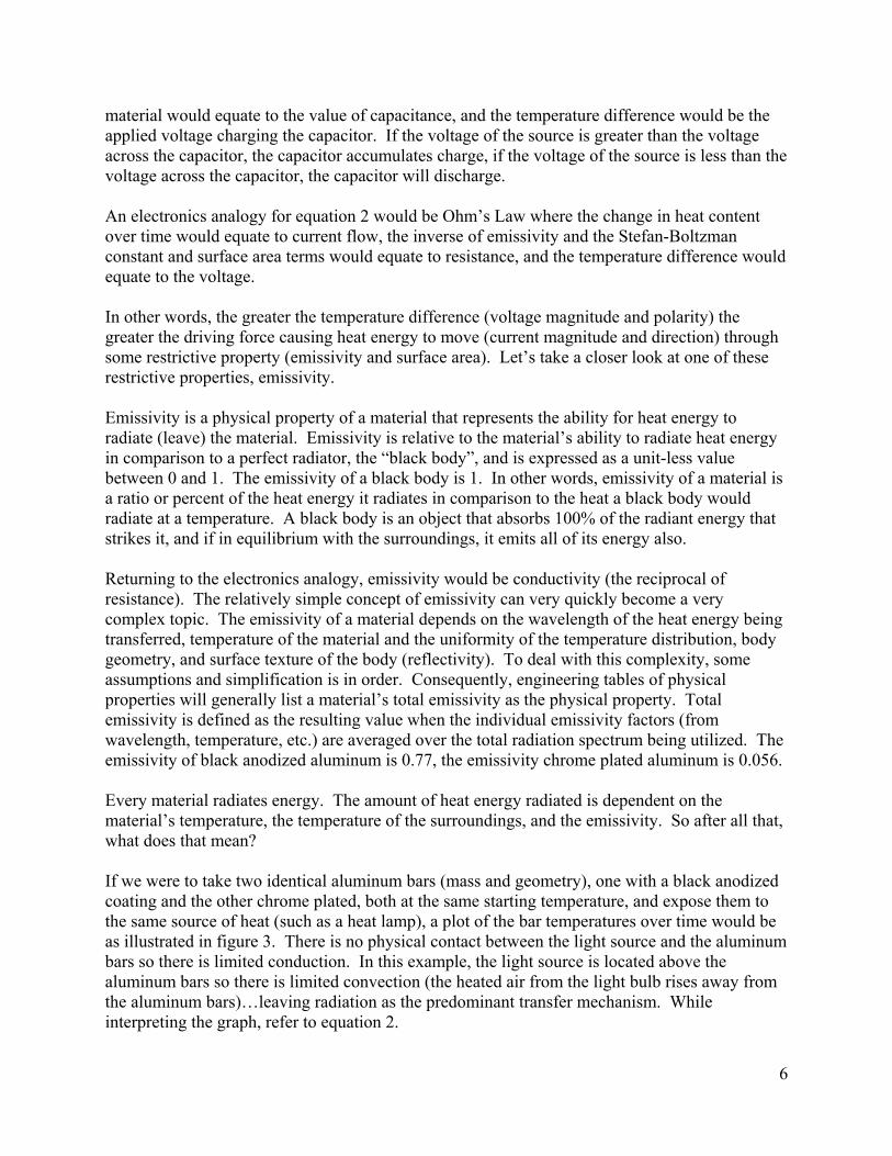
A thermopile is a device that contains a serially-interconnected array of thermocouples. One set of thermocouples are imbedded in a black body like substrate for absorbing the infrared radiation which raises the temperature detected by the thermocouple according to the intensity of the incident infrared radiation. The other thermocouple is used to measure and compensate for the temperature of the local environment. There is a small window in the end of the thermopile body that allows infrared radiation into the body. The output of the thermopile is a small voltage that is proportional to the amount of infrared radiation detected. The operational amplifier of the circuit is a simple voltage multiplier circuit that amplifies the small output voltage of the thermopile to a level more easily measured with a VOM. Figure 3 illustrates the Leslie’s Cube detector hardware. The thermopile device is mounted in the a section of a drinking straw, the position of the battery on the bottom of the board makes for a convenient sensor height to allow the detector to rest on the table surface in front of the cube portion of the system. The pins on the right side of the board are for connecting the Volt-Ohm-Meter (VOM) probes.

22

Figure 3.

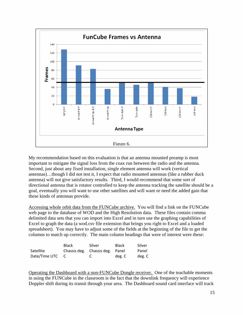
FUNCube Leslie’s Experiment Results

Surface Thermopile Voltage Emissivity Black Semi-gloss 0.80 Al Rough 0.07 Al Natural Surface 0.039-0.057 Al Foil Cover 0.04

Figure 4.

FUNCube Leslie’s Experiment Results

Surface Thermopile Voltage Emissivity Black Semi-gloss 5V (rail) 0.80 Al Rough 1.4V 0.07 Al Natural Surface 1.04V 0.039-0.057 Al Foil Cover 1.02V 0.04

Figure 5.

Conducting the Leslie’s Cube Experiment. The Leslie’s Cube experiment is relatively easy to conduct and happens very quickly. Figure 4 illustrates a data table that should be developed for recording the observations during the experiment. The emissivity column comes from standard engineering tables that list the physical properties of materials. Heat an appropriate quantity of water to a boil using a household tea kettle (use precautions when working with hot water). Set the cube on a table surface and locate the detector about ½ inch away from the cube with the thermopile facing the cube. Fill the cube with hot water and allow the metal cube temperature stabilize (it will not take very long, aluminum is a good conductor of heat). Take voltage measurements and fill in the data table. Using a gloved hand (remember the cube gets hot), rotate the cube so the next surface is facing the detector with the same distance between the detector and the cube…take and record the next voltage. Repeat quickly the other two measurements (work quickly so that there is minimum loss of heat from the water). Your results should look something like illustrated in figure 5.

23

Interpreting the results. In the Leslie’s Cube experiment, the interior walls of the cube and the interior aluminum that makes up the walls are at the same temperature because of the good thermal conductivity of aluminum. The voltage produced by the thermopile is proportional to the heat energy being radiated by the target material, so the higher the voltage the higher the amount of heat energy radiated. The connection to the FUNCube MSE is that the black bar has an emissivity of approximately 0.77, the chrome bar has an emissivity of approximately 0.056. Consequently, the black bar should gain heat and in turn radiate its heat energy more efficiently than the chrome bar. This means there will be an increase the black bar’s internal temperature (the temperature reported in the telemetry) more quickly when illuminated, and lower the black bar’s internal temperature more quickly when in eclipse when compared to the chrome bar. One artifact of the electronic circuit is the high voltage of 5 volts of the black semi-gloss surface. In this specific case, the surface temperature of the black surface was so high that the thermopile produces the maximum voltage possible for the circuit (thus the 5 volt rail). If the circuit was capable, the actual voltage produced would be greater than the 5 volt limit. If desired, you can mitigate this limitation by placing the detector at a distance that produces a black surface voltage that is within the voltage range of the detector circuit (move it further from the cube). Another experiment with the Leslie’s Cube. The power of an electromagnetic wave traveling in space follows the ‘inverse square’ of the distance from the source rule. Think of a fixed amount of electromagnetic power being emitted by a source. As the wave moves out from the source, the fixed amount of power is spread out about the surface area of a sphere (the wave front surface), the area of the sphere increases according to this formula:

4 equation 2.

And the fixed power is distributed about this surface area according to:

equation 3.

In other words, the power at a specific point drops off as the inverse square of the distance from the source. Heat energy being emitted by radiation in the Leslie’s Cube is an electromagnetic wave. If you repeat the Leslie’s Cube experiment focusing on the black surface, and record the voltage (radiated heat energy) at specific intervals as you move the detector away from the cube surface, you can demonstrate the inverse square rule. Figure 6 shows the plot of a quick experiment. The solid line is the plot of the data, the dotted line is the plot of a curve fit of the data that shows that the collected data behaves proportionally to an inverse square equation.

24

Figure 6.

Some related emissivity and thermodynamics inquiries. If you want to take your Leslie’s Cube and the FUNCube MSE a little further and connect the content to the student’s real world personal experiences, how about asking these questions (just to list a few):

How do we feel heat energy from the Sun? In an eclipse of the Sun, the heat and light from the Sun are cut off at the same moment,

what would you expect to feel? How does a greenhouse keep the heat in it? How is that related to the greenhouse gasses

that you hear about on the evening news reports? In the summer, greenhouse widows are often painted white…why? Electric and gas fire places have shiny reflectors behind them…why? Homes in hotter countries are often painted white or are made from light colored

material…why? A highly polished stainless steel teapot will take longer to cool down than one of the

same size that has a rough and/or dark surface…why? A vacuum thermos bottle has shiny interior surfaces…why? The cooling fins on a motorcycle engine cylinder head should be painted black…why?

Summary. The FUNCube MSE is an opportunity for students to experience heat transfer by radiation using a satellite orbiting in space. This is an excellent resource to supplement the study of thermodynamics in classroom, done in the traditional way, using the Leslie’s Cube experiment. In this segment of the Guide, an affordable Leslie’s Cube experiment system was detailed that the students can build and then use to study the concept of emissivity. In the next installment of the Guide another simple and inexpensive in-class experiment is described to study the absorption side of thermodynamics.

25

26

4. The MSE In-classroom Simulator (that you can duplicate) Introduction. The Leslie’s Cube experiment allows your students to explore the concept of emissivity by looking at heat radiating from a body. In this installment a very simple experiment is describe that you can easily duplicate in the classroom to explore the concept of emissivity by looking at heat absorbed by a body. Hardware. The hardware for this experiment will simulate the MSE bars as closely as possible. The materials needed to perform this experiment include:

Small identical pieces of plate aluminum (1/8th inch thickness) that is available from your local home improvement store. 

Two thermistors (Digi‐key part number 317‐1306‐ND thermistor are used here). 

Epoxy glue. 

Aluminum foil. 

Black spray paint. 

A piece of Styrofoam sheet to use as a thermal insulator. 

A desk light fixture with a small (60 watt) incandescent light bulb.  The desk light fixture should have a convenient on/off switch and should be able to hold a position over the table surface you will be working on. 

A stop watch. 

A VOM. 

Computer with Excel ® or other software capable of producing graphs. 

A refrigerator.  

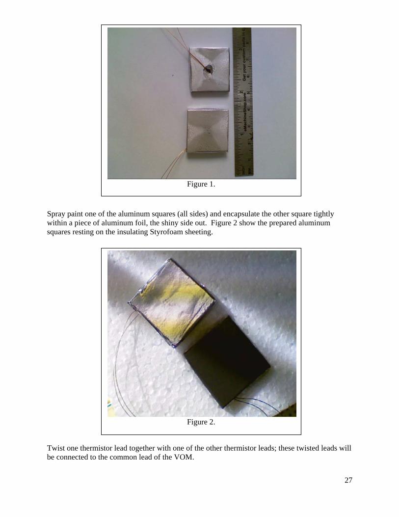
To duplicate the experiment as illustrated here, cut two pieces from the plate aluminum to create 1 inch squares from 1/8th inch stock. In the middle of one face of each aluminum square, drill a small divot hole large enough to accept the head of the thermistor. Use care not to drill through the 1/8th inch stock. Place one thermistor in each divot and hold the thermistor in place by applying some epoxy glue. Make sure the thermistor makes contact with the aluminum metal surface and is not insulated from the aluminum by epoxy. Figure 1 shows the thermistors glued in place.

27

Figure 1.

Figure 2.

Spray paint one of the aluminum squares (all sides) and encapsulate the other square tightly within a piece of aluminum foil, the shiny side out. Figure 2 show the prepared aluminum squares resting on the insulating Styrofoam sheeting. Twist one thermistor lead together with one of the other thermistor leads; these twisted leads will be connected to the common lead of the VOM.

28

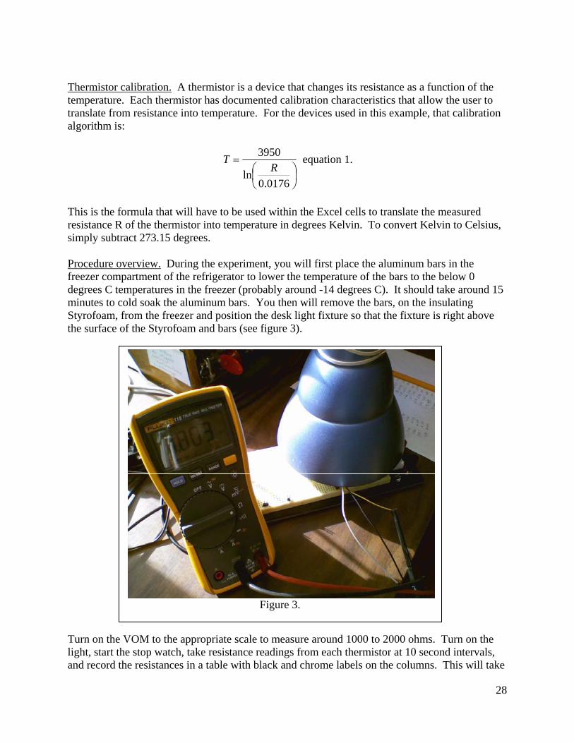
Figure 3.

Thermistor calibration. A thermistor is a device that changes its resistance as a function of the temperature. Each thermistor has documented calibration characteristics that allow the user to translate from resistance into temperature. For the devices used in this example, that calibration algorithm is:

0176.0ln

3950R

T equation 1.

This is the formula that will have to be used within the Excel cells to translate the measured resistance R of the thermistor into temperature in degrees Kelvin. To convert Kelvin to Celsius, simply subtract 273.15 degrees. Procedure overview. During the experiment, you will first place the aluminum bars in the freezer compartment of the refrigerator to lower the temperature of the bars to the below 0 degrees C temperatures in the freezer (probably around -14 degrees C). It should take around 15 minutes to cold soak the aluminum bars. You then will remove the bars, on the insulating Styrofoam, from the freezer and position the desk light fixture so that the fixture is right above the surface of the Styrofoam and bars (see figure 3). Turn on the VOM to the appropriate scale to measure around 1000 to 2000 ohms. Turn on the light, start the stop watch, take resistance readings from each thermistor at 10 second intervals, and record the resistances in a table with black and chrome labels on the columns. This will take

29

some practice. At the end of 20 minutes, turn off the light, leave the light fixture in place, but continue to record the resistances for an additional 20 minutes. Step-by-step procedure.

1. Practice placing the aluminum bars resting on the Styrofoam insulating sheet under the desk lamp fixture.

2. Set the scale of the VOM to the appropriate range for your thermistors. Readings at room temperature will give you a good idea of the appropriate scale.

3. Create a data table with Time, Black Bar, and Chrome Bar as the column headings. 4. Place the bars and Styrofoam sheet in the freezer compartment for 15 minutes. 5. As expeditiously as possible, remove the bars and Styrofoam sheet from the freezer

compartment and place under the desk light fixture. Turn on and connect the VOM. 6. Start the stop watch and turn on the light, record the thermistor resistances for time zero. 7. At 10 second intervals, measure and record the thermistor resistances for 20 minutes. 8. After 20 minutes, turn off the light but continue to record the resistances at 10 second

intervals. 9. Enter the data into Excel, use the appropriate conversion algorithm to convert resistance

into degrees C. 10. Graph the data.

The outcome of the experiment. The results of this simple experiment are very impressive as can be seen by the graph in figure 4 (you have seen this graph in the thermodynamics review section). The black line is the data associated with the black bar, the gray line is data associated with the chrome bar. Reading the graph from left to right, at time zero, both bars start out at 20 degrees C (yours should start at below zero). As the bars are exposed to the light, they gain heat as

Figure 4.

30

Figure 5.

indicated by the increase in temperature. As discussed previously, because the emissivity of the black bar is 0.77, it will gain heat at a more rapid rate than the chrome bar with an emissivity of 0.056; this relationship is clearly indicated in the graph. At the point when the light is turned off, the black bar temperature was around 110 degrees C, the temperature of the chrome bar is around 55 degrees C (with the bars of equal mass, the more heat content, the higher the temperature). When the light is on, this simulates when AO-73 is illuminated by the Sun. Continuing further right, when the light is turned off, the bars begin to radiate heat to the local environs and as the heat content of the individual bars drops, the temperatures decrease. Again, because of the differences in emissivity, the black bar loses heat at a faster rate than the chrome bar, but in the end, both bars return to room temperature. You will receive very good results doing the data collection manually, especially when there is a small group of students who are assigned specific duties to help share the work load during an admittedly busy time. The quality and reliability of the experiment can be improved by automating it a bit. A more automated experiment set up could include a programmed a PIC microcontroller that has the ADCs programmed to read the thermistor resistances (actually the voltage drop across the resistors) at 10 second intervals and in turn send the resistance readings to a computer running a terminal program (Putty) via a USB to PIC connection. Figure 5 is an example PIC microcontroller based interface. The data is then saved in a text file and eventually imported into Excel as a comma delimitated file. The details of this modification of the basic experiment is beyond the scope of this Guide, but specifics of the modification are available from the Guide author upon e-mail request (mspencer@arrl.org).

Summary. We have covered receiving the MSE telemetry transmitted by AO-73, the Leslie’s Cube experiment to explore the relationship of emissivity to heat transfer by radiation, and in this installment a simple experiment to explore the relationship of emissivity to heat transfer by absorption and radiation. In the next installment of the Guide, we’ll take a look at a few ways to interpret the actual data collected from the FUNCube MSE.

31

5. Interpreting real FUNCube MSE Data Introduction. It is now time to interpret the data from the MSE. You have done the preparatory study and review of heat transfer by radiation using the Leslie’s Cube Experiment and the MSE In-class Simulator Experiment, you have your satellite ground station running and receiving telemetry data directly from the FUNCube, and you have some actually AO-73 MSE data from one of the available sources, direct reception or web based archive…this is where the real learning begins. In this installment, just a few of the possible uses of the data will be explored, there are many, many more opportunities afforded by participating in the MSE, consider this just the beginning. What is happening; on the meta-level (thinking about what it is like in orbit)? It is helpful to anticipate the environment on orbit that AO-73 is experiencing. In turn, this “thinking about space” will set the stage for forming some hypotheses that can be used as the framework to evaluate the data being collected by the MSE. Let’s review some of the things we know about AO-73 and the MSE.

1. There are two sets of bars mounted on the satellite that make up the MSE. These bars are made of aluminum and coated with a black anodized surface or a polished chrome surface.

2. The emissivity’s of the bars are approximately 0.77 for the black anodized bar and 0.056 for the chrome plated bar.

3. One set of four bars are mounted in the corners of the satellite cube structure and are part of the cube structure. These bars are not thermally isolated from the cube body therefore heat transfer by conduction will be a significant. These bars are identified as Black and Chrome Chassis Temp in the Dashboard.

4. One set of two bars are mounted on the -X-axis face of the cube and they are thermally isolated from the satellite structure. Heat transfer by conduction or convection is minimal for these bars. These bars are identified as Black and Chrome Panel Temp in the Dashboard.

5. There are thermistors mounted in each of the bars. The internal temperatures of the bars are measured and reported via telemetry at 60 second intervals.

6. There are Sun Sensors mounted on all the satellite surfaces except on the –X surface (where the MSE panel bars are mounted). These sensors are monitored at 1 second intervals for one minute, and not monitored for a one minute pause period. The output of the Sun Sensors is also reported as High Resolution telemetry.

7. There are a number of other sensors and satellite housekeeping parameters measured and reported via telemetry (but these additional sensors and readings will be left for future study).

8. The satellite is orbiting in a near polar orbit. The satellite goes through a period of illumination from the Sun during a portion of the orbit, and is eclipsed from the Sun (in the Earth’s shadow) during the other portion of the orbit. The orbit period is on the order of 104 minutes.

9. The satellite is rotating about the Z-axis of the satellite (the vertical axis for reference) exposing the X, Y surfaces of the satellite more toward the illumination of the Sun. There is in all likelihood some oscillation or wobble about the Z-axis during the rotation (think of a spinning top).

32

Figure 1.

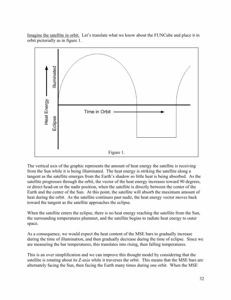
Imagine the satellite in orbit. Let’s translate what we know about the FUNCube and place it in orbit pictorially as in figure 1. The vertical axis of the graphic represents the amount of heat energy the satellite is receiving from the Sun while it is being illuminated. The heat energy is striking the satellite along a tangent as the satellite emerges from the Earth’s shadow so little heat is being absorbed. As the satellite progresses through the orbit, the vector of the heat energy increases toward 90 degrees, or direct head-on or the nadir position, when the satellite is directly between the center of the Earth and the center of the Sun. At this point, the satellite will absorb the maximum amount of heat during the orbit. As the satellite continues past nadir, the heat energy vector moves back toward the tangent as the satellite approaches the eclipse. When the satellite enters the eclipse, there is no heat energy reaching the satellite from the Sun, the surrounding temperatures plummet, and the satellite begins to radiate heat energy to outer space. As a consequence, we would expect the heat content of the MSE bars to gradually increase during the time of illumination, and then gradually decrease during the time of eclipse. Since we are measuring the bar temperatures, this translates into rising, then falling temperatures. This is an over simplification and we can improve this thought model by considering that the satellite is rotating about its Z-axis while it traverses the orbit. This means that the MSE bars are alternately facing the Sun, then facing the Earth many times during one orbit. When the MSE

33

bars are facing the Sun, they receive heat energy directly from the Sun, when the MSE bars are facing the Earth they are receiving a reduced amount of heat energy that is reflected off the Earth’s outer atmosphere. Figure 2 is a modified model that includes a rotating satellite. Depicted here are the darker humps that represent when the MSE bars are facing the Sun and receiving more heat energy, the lighter, dotted humps represent when the MSE bars are facing the Earth and receiving less and reflected heat energy. The cosine curves of the humps are over emphasized to illustrate the point. Again, while in eclipse, the satellite is not receiving heat energy from the Sun. With this modification of our though model we would expect that the temperature rise during illumination would be less than what the temperature rise would be if the satellite were not rotating. Referring back to the temperature profile that was produced by the MSE In-class Simulator detailed in the previous segment (Section 1, figure 3), you can see a good correlation between our ‘thought’ model and the data produced by our MSE In-class Simulator. [We would also expect that the actual temperature curve in illumination would not be a smooth curve but oscillating above and below the smooth curve as the satellite face rotates into and out of the Sun.]

Figure 2.

34

In this case, the differences in emissivity between the black and chrome bars are evident. During illumination, as heat energy is absorbed, the temperature rises (but differences in emissivity cause the temperature rises to be dissimilar), during eclipse, as heat energy is radiated, the temperature decreases. Our first look at real MSE data. Let’s look first at the whole orbit data produced by the chassis mounted bars (those in the corners of the cube) of the MSE. The data could have been obtained by direct reception of the telemetry or it could have been obtained by downloading the data from the central database of data. The graph could have been generated by Excel, the graph could have been generated by the Dashboard, or generated and displayed on the FUNCube web page. The illustration in figure 4 was generated by inserting the WOD from the database into Excel. There is a lot of information contained in the graph; we’ll use some speculation and educated guesses to gain some meaning from the graphs. First, there is remarkable similarity between the actual plot and the plot obtained using the MSE In-class Simulator. The most significant departure is that there is no real difference between the curves of the black bar and the chrome bar. This disconnect however can be rationalized by the fact that in the chassis bar installation, the bars are integral to the satellite structure and not thermally isolated from the rest of the satellite structure. This means that heat transfer by conduction to the rest of the parts of the satellite is significant in comparison to the heat transfer by radiation. Therefore the heat transfer by conduction would tend to mask the heat transfer by radiation and equalize the temperatures. Second, look at the temperature “hump” indicated at location A, approximately half way between leaving and then reentering the eclipse of the orbit. At point A, the vector of the heat energy from the Sun is near nadir, and at this point of direct illumination of the bars, you would expect the heat energy absorption to be the greatest.

Figure 3.

35

Figure 4.

Third, look at the temperature “nulls” indicated at location B. The Z-axis of the satellite is maintained roughly in parallel with the lines of the Earth’s magnetosphere by fixed, permanent magnets aligned with the Z-axis of the satellite. These magnets actually cause the satellite to “flip” over, about the Z-axis, two times during the course of a single orbit to keep the antennas optimally aligned with the Earth to help facilitate communications between the Earth ground stations and the transponder on the satellite. During the flip maneuver, the X and Y axis of the satellite are not optimally exposed to the Sun, and it appears that one of these flip periods are showing up as the shallow nulls at point B in the orbit.

Fourth, the next interesting observation is the deviation from a smooth temperature curve. The oscillations about the imaginary smooth curve are greater for the black bar than for the chrome bar as highlighted at point C in the graph. This is one artifact of the differences in emissivity of the bars and heat transfer by radiation in spite of the transferance by conduction dominating. If you take a close up look at the period of the oscillations, you would note that they match the expected rotation rate of the satellite. Consequently, when the bars are facing toward the Sun, heat transfer by radiation is greatest, when facing the Earth, heat transfer is less. The overall deviation of the oscillations of the black bar plot is greater because the emissivity of the black bar is greater. Figure 5 illustrates another way of using the whole orbit data, in this case using a plot generated from the Dashboard. This is the plot of the X panel voltage generated by the solar panel on that surface. It is very clear and evident when the satellite emerges from the eclipse, when the output

36

Figure 5.

Figure 6.

voltage is high, and when the satellite enters into the eclipse, when the voltage drops to virtually zero. This is a good graphic to correlate to the other graphs, such as figure 4, to show when the eclipse starts and ends.

Using the high resolution data to determine satellite rotation rate. Figure 6 is an example where you can use the high resolution graph from the Sun Sensor data generated with the Dashboard to determine the rotation rate of the satellite. This is where the number of decoded frames becomes important. If there are insufficient decoded frames, there might not be enough information contained in the graph to give you the complete picture you need to infer the rotation rate. This graphic was generated from a pass that produced over 90 decoded frames (basically a fully decoded data set).

Let’s take a moment and look at what the graph is displaying. The Sun sensors produce an output value that is proportional to the intensity of the Sun’s illumination of the satellite’s face. The peak, flattop region is where the face of the satellite is in full Sun. As the satellite face rotates out of direct Sun illumination, the value falls off to the minimum. Also, the data that is collected is interrupt by pauses, the Sun sensor output is sampled every second for one minute,

37

then there is a pause of one minute before the next collection period. The one minute periods are annotated on the graph. There is one complicating problem that at the time of this writing has not been resolved. The X-axis of the graph is the clock time in UTC. The only time that the time reported on this axis is close to accurate is immediately after a live collection and display. If you save and replay the session later, as was done to produce this illustration, the X-axis time is not correct, in fact, it is not even scaled correctly. This issue will probably be corrected in future updates of the Dashboard software, but in the mean time, use caution when pulling time intervals from the X-axis and make adjustments accordingly (this is why the minute time interval was stressed, it can be used to properly scale the X-axis of the graph from the data set points). Returning to figure 6, notice the location of when the satellite face enters the shadow, the dramatic drop in value. If you simply take the difference in time between these drop-off points, you can calculate the rotation rate of the satellite. At the time of the data collection, the rotation rate was approximately 2.5 minutes per revolution. Notice also, that the rises when the sensors enter the Sun light are missing in the plot. This is due to the minute on/minute off collection scheme (the difference between this 2 minute collection cycle and the 2.5 minute rotation rate of the satellite). Over the course of the orbit, both the rise and fall points will be displayed, then a little further in the orbit, only the rise points will be displayed and the fall points will be missing. This is similar to what you see when you observe a spoked wheel in a movie, when the speed of rotation of the wheel and the shutter rate of the movie camera are just right, the spoked wheel appears to be rotating backwards. Using the high resolution data to determine satellite Z-axis wobble. The behavior of the satellite about the Z-axis is complicated and very interesting. As mentioned, to maintain desired orientation, the satellite is flipped about the Z-axis through the passive means of permanent fixed magnets to align the Z-axis approximately to the lines of the Earth’s magnetosphere. By monitoring the Z-axis Sun Sensor high resolution data, you could possibly determine the “wobble” rate and magnitude, and longitudinally, see if the wobble rate and magnitude change over time (figure 7).

38

Figure 8.

Figure 7.

Correlating Sun Sensor and Solar Panel Temperature data. Here is an example of an Excel display that overlays the Sun sensor data with the solar panel temperature data. In Figure 8, the black line is the Sun sensor data, the gray line is the solar panel temperature. There is a clear correlation between the Sun illuminating the panel, but with a hysteresis shift that delays the temperature rise of the panel to immediately follow the illumination by the Sun.

Hysteresis is a common phenomenon in science. In climatology, your students may have noticed the lag of average temperatures behind the Winter and Summer solstices when the Sun’s illumination of our hemisphere is either at the peak or minimum yet the associated peak and minimum average temperatures arrive a month of so after the solstices.

39

Figure 9.

Returning to the elephant in the room. At the end of the first segment of the Guide, an unanticipated disconnect between the whole orbit data and what was expected was obvious, it is time to revisit that disconnect. Take a quick look again at figure 3, think back to the discussion of thermodynamic fundamentals from the first installment, and then study the graph of the whole orbit data for the other portion of the MSE, the panel mounted bars which are thermally isolated and mounted on the face of the –X axis of AO-73 (figure 9).

The first striking observation is that the chrome bar temperature prior to entering eclipse (the middle of the graph) is greater than the black bar temperature; even when considering that the starting temperature of the chrome bar is a few degrees warmer than the black bar. Then, early in the plot, the slope of the black bar temperature rise is greater than the chrome bar as would be expected, but about the point of maximum Sun illumination during the orbit, the plots cross, the slopes converge, and then the slope of the chrome bar temperature becomes greater than the black bar temperature slope. This clearly is counter to the behavior one would expect based on the outcome of the MSE In-class Simulation as depicted in figure 3, and supported by the thermodynamics review of the first installment. There are some consistent results. If the temperature curves in eclipse are biased so that the starting temperature of the chrome bar is the same as the black bar, the temperature profile in eclipse is approximately the same, and consistent with what is observed in the whole orbit data of the chassis mounted bars (figure 10).

40

Figure 10.

Figure 11.

Another informative way to look at the disconnect between the expected heat energy transfer and the real heat energy transfer is by looking at the oscillations of the curves that result from the rotation of the satellite. The period of the oscillation is identical to what we had seen in figure 4. If we take a closer look at the rate of temperature change (the derivative of the curves) and the amplitude of the temperature oscillations, we can quantify the resulting difference between the ending temperatures of the black and chrome bars (figure 11, generated by Excel).

41

Figure 12.

Graphing the derivative of the curves, we are comparing the rate of energy change between the bars, and taking the average of the rates of energy change, we are comparing the end heat energy content. It is clear in the graph that the energy transfer rate excursions (+ above, - below the smoothed curve) of the black bar are greater than in the chrome bar. This is consistent with the differences in emissivity. The black bar, with the higher emissivity gains, and loses, energy at a greater rate than the chrome bar with a lower emissivity. Yet, by taking the average rate of change over time, the chrome bar had an average positive rate of 0.420 in comparison to the average positive rate change of the black bar of 0.408. This is not consistent with the differences in emissivity (it should be the other way around) and suggests that the rate of energy change oscillations that are due to the rotating satellite may be responsible for the chrome bar’s departure from the predicted behavior. Returning to the MSE In-class Simulator. So on one hand the MSE outcome behaves as expected when the environment is close to equilibrium or steady state (during eclipse). On the other hand the MSE outcome does not behave as expected when the environment is dynamic (during illumination and a rotating satellite). In using the MSE In-class Simulator previously to demonstrate the absorption principles, the environment was close to equilibrium or steady state because the light was turned on, and left steady on, then turned off. The outcome of the experiment was as expected as shown in figure 3. We can take the MSE In-class Simulation into the dynamic realm and simulate a rotating satellite by modulating (turning on and off) the light and repeating the experiment. In this first instance, the light was turned on and off at 30 second intervals for 20 minutes. Following the same procedures, the resistance of the thermistors was measured and recorded at 10 second intervals and the data graphed for analysis. The duty cycle of the illumination is 50%, in other words, the bars are receiving half the heat energy. The results are shown in figure 12. Compare this graph to the illumination side of figure 3.

42

Figure 13.

First, notice that there are temperature deviations (oscillations) with a period of 1 minute (2 x 30 seconds). The +/- deviations from the black bar smoothed curve are approximately equal. Also notice that the deviations of the chrome bar are far smaller in amplitude than the deviations of the black bar. This is consistent with the differences in emissivity. However, notice the difference in the ending temperatures. In this dynamic experiment the black bar is approximately 40 degrees warmer than the chrome bar. Alternatively, the temperature difference between the bars in the original equilibrium experiment was 50 degrees. It is interesting that the overall temperatures approximate the 50% duty cycle of the heat energy source, but the temperature difference between the two bars appears to trend toward convergence. In the second instance, the experiment is repeated using a 60 second interval. This experiment approximates the illumination interval of AO-73 in orbit (2.5 minutes). The result is shown in figure 13.

Notice the deviations from the smooth curve are greater for the black bar, are clearly visible in the chrome bar plot, and have a period of 2 minutes. Most significant; notice that the ending temperature difference between the black and chrome bar is reduced to approximately 25 degrees meaning the curves are converging (Δ 50o - Steady State; Δ 40o - 30 Sec; Δ25o - 60 Sec) . This is inconsistent with the Stefan-Boltzman Law. The outcome of the MSE In-class Simulation suggests that there are dynamic conditions when the temperature profile of the lower emissivity chrome bar could cross the temperature profile of the higher emissivity black bar (which of course is observed in the real data).

43

Figure 14.

This is pure speculation and conjecture deserving a lot more thought and investigation: one possible explanation is, it would appear, that in dynamic conditions, the black bar radiates the heat energy at a greater rate than it absorbs, and the chrome bar absorbs heat energy at a greater rate than it radiates, and therefore, over time, the curves converge, cross and the chrome bar ends up at a higher temperature. This would indicate that the emissivity and the absorptivity of the black bar are not necessarily equal in a dynamic condition, as stipulated in the definition of the black body. Alternatively, the absorptivity of the chrome bar is greater than the emissivity by some detectable amount and would indicate that the chrome bar does not behave as a black or gray body in a dynamic situation. If we combine the three MSE In-class Simulations in one graphic (figure 14), observe that as the period of illumination goes from steady state, to 30 seconds, and then to 60 seconds (i.e., the situation becomes more dynamic, more of a departure from steady state) that the ending temperatures of the black and chrome bars migrate toward each other, tend to merge. As stated in the thermodynamics refresher section of the first installment, the emissivity of a material is complex and depends on the wavelength of the heat energy being transferred, temperature of the material and the uniformity of the temperature distribution, body geometry, surface texture of the body (reflectivity), but as indicated by the MSE results, it also depends on the dynamic nature of the situation and the emissivity’s departure from the black body value of 1. The graphic of figure 15 pictorially illustrates the complex relationship between emissivity, absorptivity, and departure from the black body.

44

Figure 15.

It would appear that in the MSE, the assumption that the black bar with an emissivity of 0.77 behaves as a black or gray body in the dynamic conditions of a rotating satellite in orbit is not necessarily correct. The MSE seems to indicate that in a dynamic situation, the location of the black bar on the emissivity-absorptivity continuum illustrated in figure 15 moves toward the right, while the location of the chrome bar on the continuum moves toward the left, the result is the chrome bar attaining a higher temperature. Again, pure speculation and conjecture worthy further study. Summary. There are huge learning opportunities contained in the FUNCube MSE, we have only scratched the surface. It is clear that there is a risk of over simplifying what is going on with the FUNCube MSE, but going beyond simplification and taking the risk provides an opportunity to take the thermodynamics concepts explored during the MSE to a much higher level of learning. Yes, the Dashboard produces some very easy, and impressive graphs. But if that is as far as the MSE is taken, there are many questions, and possible answers, that would be missed…arguably the questions being more important than the answers. There are probably many readers who consider this segment to be “oh-hum” material not “ah-ha” material, and perhaps downright wrong and misleading. It however is up to the instructor to put this material, and the FUNCube MSE, into a context that helps their students gain from the experience. Let the students explain what they observe…that is where the real learning begins…even if they are only half right, or even if they are wrong. The final installment of the Guide will suggest some other learning opportunities afforded by the FUNCube MSE.

45  

6. Further studies using MSE data Guide Conclusion. The basic theme of the Guide has been that the FUNCube MSE is an exceptional instructional resource that can be accessed very affordably. The Guide has only scratched the surface of the FUNCube’s potential, there are many, many more possible learning opportunities afforded by this resource. These additional activities can be lump-grouped into three basic categories; longitudinal studies that occur over a period of time, discrete studies that can be conducted with a single, or just a couple, observations, and additional in-class experiments that simulate conditions and behaviors on-orbit using systems or simulations such as the Leslie’s Cube or the MSE In-class Simulator detailed in the Guide. Below are just a few examples of activities that are possible, the list is offered only to stimulate your own list. Longitudinal (over time) studies.

l1 Monitor the change in emissivity of the individual bars over time to see if there is a degradation of the surfaces.

l2 Monitor for changes in the rotation rate of the satellite.

l3 Monitor for changes in solar panel operating temperatures.

l4 Monitor for changes in emissivity of the MSE bars.

l5 Monitor for changes in battery performance.

l6 Monitor for changes in Z-axis “wobble”.

l7 Determine Frequency drift as a function of Keplarian data quality and frequency of

updates.

l8 Verify the RF link power budget as a function of maximum elevation by direct signal strength observations.

l9 What is the maximum panel bar temperature versus the rotation rate?

Discrete studies (one time or short period) studies.

d1 Determine the direction of rotation of the satellite.

d2 Compare and contrast the heat loss to space versus the heat loss/gain to/from Earth.

d3 Compare and contrast the thermodynamics between in sun/in eclipse.

d4 Using the chassis bars and the panel bars, compare and contrast heat loss by radiation alone and radiation/conduction.

46  

d5 Determine the temperature of the Sun’s surface.

d6 Determine the effective temperature of deep space.

d7 Determine the effective temperature of the Earth’s upper atmosphere.

d8 Measure the temperature of the Earth’s upper atmosphere as a function of latitude.

d9 Determine frame decode success versus transmitter power output.

d10 Determine signal strength differences between when illuminated versus when in eclipse.

d11 Compare and contract heat transfer on the satellite via conduction and radiation.

d12 Determine solar panel temperature as a function of current draw from the solar panel.

d13 What is the battery discharge depth versus time in eclipse?

d14 What is the battery charge maximum versus time in illumination?

d15 Determine maximum temperature of various parts and components as a function of

rotation rate.

d16 Determine frequency drift as a function of temperature.

In-class experiment enhancements.

i1 Using the inexpensive Leslie’s Cube and the thermopile, explore the concepts of heat transfer via radiation and the effects of emissivity of more varied and different texture surfaces.

i2 Determine the emissivity of the individual bars from the temperature data.

i3 Determine satellite pass maximum elevation distribution.

i4 Determine the average velocity of the satellite.

i5 Determine the average altitude of the satellite.

i6 Determine the average altitude of apogee.

i7 Determine the average altitude of perigee.

i8 Determine the Drift rate of the apogee location.

47  

i9 Determine the RF link power budget as a function of maximum elevation.

i10 What is the maximum rotation rate that can be profiled with the Sun Sensor sample rate scheme?

i11 What combination of lamp intensity (wattage), frequency (standard incandescent versus

IR heat lamp), light on/off frequency and period, and different surface coverings of the bars give results where the two temperatures cross and more closely mimic the actual behavior of the bars on orbit?

Summary. AMSAT-UK provided the resource, the Guide has shown you that you can affordably access the FUNCube MSE, and it has illustrated some of the Science and Mathematics content that you can bring into your classroom; it’s now up to you to make it happen. Your efforts will be well rewarded in your students learn while exploring space with the FUNCube MSE.