1

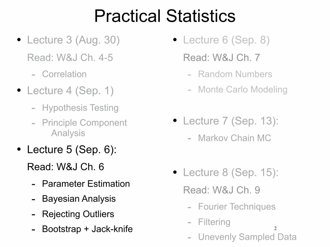
Practical Statistics • Lecture 3 (Aug. 30)

Read: W&J Ch. 4-5

- Correlation

• Lecture 4 (Sep. 1) - Hypothesis Testing

- Principle Component Analysis

• Lecture 5 (Sep. 6): Read: W&J Ch. 6

- Parameter Estimation

- Bayesian Analysis

- Rejecting Outliers

- Bootstrap + Jack-knife

• Lecture 6 (Sep. 8) Read: W&J Ch. 7

- Random Numbers

- Monte Carlo Modeling

• Lecture 7 (Sep. 13): - Markov Chain MC

• Lecture 8 (Sep. 15): Read: W&J Ch. 9

- Fourier Techniques

- Filtering

- Unevenly Sampled Data2

General Picture:

Correlation -> Hypothesis Testing -> Model Fitting -> Parameter Estimation.

Is there a correlation? Is it consistent with an assumed distribution? Does the assumed model fit the data? What parameters can we derive for the model with what

uncertainty?

3

guessthecorrelation.com

Parameter Estimation

Most data analysis has the final goal of estimating the value (and uncertainty) of a parameter or parameters.

The modeling portion of this seeks to find the parameters which have the maximum probability of generating the observed data.

The assumption of this approach is that the model (and error estimates) are valid. Alternatives should be explored.

4

P =Y

i

f(xi|�)

Maximum Likelihood

If we know (or can guess) the probability distribution,f(alpha), of our data, then we can write for our set of data:

5

The maximum of this function gives us our best estimate of the parameters, alpha.

Example of Using Maximum Likelihood.

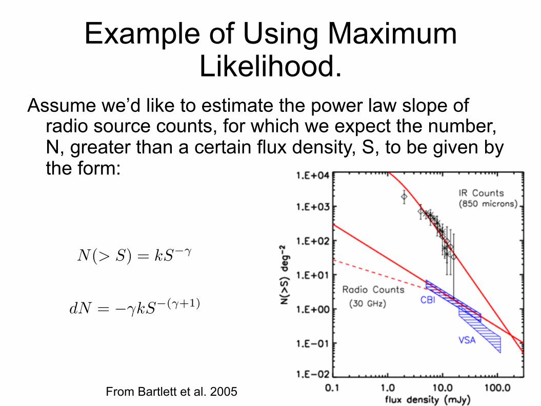
Assume we’d like to estimate the power law slope of radio source counts, for which we expect the number, N, greater than a certain flux density, S, to be given by the form:

6

From Bartlett et al. 2005

N(> S) = kS��

dN = ��kS�(�+1)

Example of Using Maximum Likelihood.

7

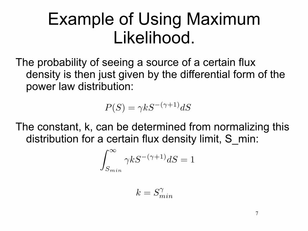
The probability of seeing a source of a certain flux density is then just given by the differential form of the power law distribution:

The constant, k, can be determined from normalizing this distribution for a certain flux density limit, S_min:

P (S) = �kS�(�+1)dS

Z 1

Smin

�kS�(�+1)dS = 1

k = S�min

Maximum Likelihood

The maximum likelihood of gamma can then be found from setting the derivative with respect to gamma (actually d ln(L)/ d gamma) to zero:

8

L(�) =MY

i=1

�S�minS�(�+1)

i

ln(L)) =MX

i=1

ln(�)� �

X

i

ln

Si

Smin+ constants

d(ln(L))d�

=M

��

X

i

lnSi

Smin= 0

�MLE =M

Pi ln Si

Smin

NX

i=1

�(yi � y(xi))2

2�2

The Classic Example: Linear Fitl What is the probability a certain data point is drawn

from a given model?

l For N points the overall probability for a given model is

l To maximize the probability we should minimize the exponent:

P / e�(yi�y(xi))

2

2�2

P /NY

i=1

e�(yi�y(xi))

2

2�2

y = b + mx

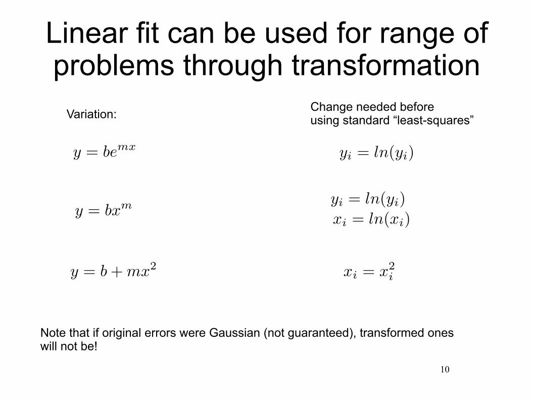
yi = ln(yi)y = bemx

y = bx

m

xi = ln(xi)

y = b + mx

2xi = x

2i

Linear fit can be used for range of problems through transformation

10

Variation: Change needed before using standard “least-squares”

yi = ln(yi)

Note that if original errors were Gaussian (not guaranteed), transformed ones will not be!

A �X = �Y

�X =

bm

��Y =

2

664

y1

y2

...yN

3

775�A =

2

664

1 x1

1 x2

...1 xN

3

775

⇥C =

2

664

�2y1 0 ... 00 �2

y2 ... 0...

0 0 ... �2yN

3

775

C�1A �X = C�1�Y

Linear Algebra Approach

You would like to solve the system of equations:

11

Where:

To do so, you weight each solution using the covariance matrix:

A

T =

1 1 . . . 1x1 x2 . . . xN

�A =

2

664

1 x1

1 x2

...

1 xN

3

775

Linear Algebra Crash Course

If we have a square matrix, A, then we can write:

12

A�1A = I

We can create a square matrix from a “m x n” matrix by multiplying by its transpose:

[AT C�1A]�1 = Cov =

�2b �mb

�mb �2m

�

... and the solution

Left-multiply by A-transpose. Isolate X

�X = [AT C�1A]�1[AT C�1�Y ]

If the errors are valid, then the first term is important:

Useful Matlab routines:zeros, ones - creates a vector or matrix of zeros or ones eye - creates identity matrix repmat - replicates a vector into a matrix cat - concatenates two vectors into a matrix plot - plots two quantities errorbar - plots two quantities with errorbars A’ - transpose of A inv(A) - matrix inverse of A C\A - matrix inverse of C times A (:,1) - a selection of all the rows and column 1 of a matrix random - generation of random number from a particular

distribution. 14

Putting MLE into Practice

Your data always has “oddities”

These “oddities” can dominate the parameter estimation

How do we remove them in an objective way?

Fast and Easy way Slow and Righteous way

15

16

Sigma-clipping

• Create best fit model.

• Define x sigma as “unlikely”.

• Get rid of points outside of x sigma

• Refit data.

• Iterate, if necessary.

17

Can be good for obvious outliers Gets murky when outliers are several sigma Can throw out good data.

Which points should get clipped?

19

Bayesian Analysis

We can develop a model that assumes the data is contaminated by bad points: Assume each point has the same probability, P_b, of being

bad. Assume these points have a mean Y_b, and variance,

V_b. with a Gaussian distribution.

Suggested Sampling of new parameters: P_b is uniform from 0 to 1 Y_b is uniform from 0 to 2*mean(Y) V_b is uniform from 0 to (max(Y)-min(Y))^2 20

Some points:

Nothing special about the choice of the distribution for the bad points, or the priors.

We need to choose something in order to make the calculations. Gaussian distributions are easy to calculate.

We will be “marginalizing” over these parameters in the end, so only want them to be reasonable approximations of the experiment.

21

The Likelihood Distribution

For the model of mixed good and bad points from two separate distribution, we end up with a likelihood distribution:

22

ML =Y

i

1� Pbq2�⇥2

yi

e�(yi�mxi�b)2

2�2yi +

Pbq2�(⇥2

yi + Vb)e�(yi�Yb)2

2�2yi

We are interested, in using this to define the “best” value of m and b, as well as it’s confidence interval.

The best value for m and b, is called the Maximum A Posterior (MAP) value.

Marginalization

We want to marginalize (or get rid of) the parameters we defined to model the bad data.

The way to do this is to numerically integrate over P_b, V_b, and Y_b for each m and b value.

The maximum in the b vs. m plot now incorporates our prior information about the data.

23

Example

24

marginalized MAP contour plot

25

Bayesian Fit

This uses all the data, and is not skewed by the outliers.26

ErrorsIf individual errors are estimated correctly, the ML can tell

us the confidence interval. If error are underestimated we can have problems! (right)

27

What about the errors?

Often the errors may be not known or are not to be trusted.

There are techniques that use only the data values (not there uncertainties) to derive the parameter uncertainty.

Two common techniques: Bootstrap Jack Knife

28

�2m =

1M

MX

j=1

[mj �m]2

Boot Strap Technique

Method: If there are N data points, randomly choose the data

point pairs, N points in each set, but can get doubles, or not use full

set. Make M data sets. Calculate variance:

29This is very flexible, being able to use any numerical

metric for “goodness of fit”

m =1N

NX

j=1

mj

�2m =

N � 1N

NX

j=1

[mj �m]2

Jack Knife Technique

Method: For a data set of N values, remove each one in turn. For each subset of data, calculate m_i Then:

30

Objective Data Modeling

Removing data is subjective and irreproducible.

Sigma clipping is a prescription, without a model of why you have the data you do.

The Bayesian analysis of outliers is an objective fit to the data, which incorporates your knowledge of the outliers.

Bootstrap and Jack knife allow robust estimation of errors. 31