Practical Session Instructions Earth Observation of Water Resources

Practical Session Instructions

Earth Observation of Water Resources (SEBS)

Prof. Bob Su & M.Sc. Lichun Wang ITC, University of Twente

The Netherlands

(July 2013)

Contents Introduction .................................................................................................................... 1 Exercise 1: Preparing MODIS Level 1B data as input for SEBS .................................. 2

1.1 Preparing software for using MODIS products ................................................... 2 1.1.1 HDFView ...................................................................................................... 2 1.1.2 ModisSwathTool ........................................................................................... 2

1.2 Ordering and downloading the data ..................................................................... 3 1.3 Getting familiar with the MODIS data with HDFView tool ............................... 5

Exercise 2: Processing MODIS Level 1B data for use in SEBS for ILWIS .................. 9 2.1 Introduction .......................................................................................................... 9 2.2 Install ILWIS and BEAM software ..................................................................... 9 2.3 Main Processing Steps ....................................................................................... 10

2.3.1 Step I: Reprojecting MODIS Level-1B Data .............................................. 11 2.3.2 Step II: Importing GeoTIFF files into ILWIS raster files ........................... 15 2.3.3 Step III: Pre-processing Tools for SEBS .................................................... 17 2.3.4 Step VI: Running SEBS core module (Surface Energy Balance System) .. 29

2.4 References: ......................................................................................................... 34 Exercise 3: BEAM plug-in for SEBS .......................................................................... 37

3.1 Generating SMAC outputs in BEAM ................................................................ 37 3.2 Generating SEBS outputs .................................................................................. 39

3.2.1 SEBS requested meteorological and radiation input values ....................... 39 3.2.2 SEBS requested satellite input files ............................................................ 40 3.2.3 SEBS Landuse Parameters .......................................................................... 42

3.3 References .......................................................................................................... 43

WATER RESOURCES (SEBS) Exercise 1

1

Introduction This practical contains three exercises related to earth observation of water resources. These exercises were developed originally for the ESA-MOST Dragon programme advanced training course in land remote sensing. Exercise 1 deals with the preparation of MODIS Level 1B data as input for SEBS, which includes preparing software for reading MODIS products, ordering and downloading the MODIS Level_1B data, and viewing and getting familiar with the MODIS data products in HDF format. Exercise 2 leads you though the different steps in processing satellite data (e.g. MODIS Level-1B data) in the ILWIS system (Integrated Land and Water Information System, an open source Remote sensing and GIS system developed by ITC, University of Twente, downloadable from http://www.itc.nl/research_programme, following the ‘ILWIS - Remote Sensing and GIS software’ link). In a step by step procedure, this exercise enables you to derive land surface geophysical parameters and energy balance components, including evaporation rate. Exercise 3 describes similar steps as in Exercise 2 but using the BEAM software environment (http://www.brockmann-consult.de/cms/web/beam/). BEAM is an open-source toolbox and development platform for viewing, analysing and processing of remote sensing raster data. BEAM supports image data from Envisat's optical instruments, raster data formats such as GeoTIFF and NetCDF as well as data formats of other EO sensors from MODIS, AVHRR, AVNIR, PRISM to CHRIS/Proba. Various data and algorithms are supported by dedicated extension plug-ins. Similarly you go though the different steps in processing satellite data (e.g. AATSR Level-1B data) to derive surface geophysical parameters and energy balance components, including evaporation rate by using the SEBS plug-in.

http://www.itc.nl/research_programme

http://www.brockmann-consult.de/cms/web/beam/

http://github.com/bcdev/beam


2

By Lichun Wang, July, 2012

Exercise 1: Preparing MODIS Level 1B data as input for SEBS In this exercise we will apply various procedures to estimate evaporation from MODIS L1B products (L1B is radiometricaly calibrated, but not atmospherically corrected data). The tasks in this exercise are to perform:

• Preparing the software for MODIS products • Ordering and downloading the MODIS Level_1B data • Viewing and Getting familiar with the MODIS data products (HDF datasets) used in

this exercise

1.1 Preparing software for using MODIS products

1.1.1 HDFView HDFView is a tool for browsing and viewing the contents of HDF files. The software can be downloaded from http://www.hdfgroup.org/hdf-java-html/hdfview/ If not installed already, installed the package as follows:

1. Type hdfview_install_windows_novm.exe to install 2. Start from Start -> programs -> HDFView 2.8 -> HDFView 2.8 Note: Before the installation of the software, Java JDK1.5.0 (or higher) must be installed on your machine.

1.1.2 ModisSwathTool The Modis Reprojection Tool Swath allows you to reproject swath MODIS level-1 and level-2 data products. It is free and can be obtained from: http://lpdaac.usgs.gov/landdaac/tools/mrtswath/index.asp In this exercise, assuming you have downloaded the software as the zip file MRTSwath.zip.

1. Unzip the MRTSwath software to a folder, for example, D:\MRTSwath directory. 2. Edit the ModisSwathTool.bat file in D:\MRTSwath\bin directory. You will need to

update the MRTDATADIR to the MRTSwath data directory, the path to the Java executable, and the path to the ModisSwathTool.jar file. For example, the Java executable path is C:\Program Files\Java\jre1.5.0_11\bin, and the MRTSwath is installed in the D:\MRTSwath directory, the sample ModisSwathTool.bat file looks like as follows:

- set MRTDATADIR=D:\MRTSwath\data - "c:\WINDOWS\system32\java.exe" –classpath

"D:\MRTSwath\bin\ModisSwathTool.jar" mrtswath.ModisSwathTool

Note that the blue statement is all on one line. Do not break this statement into multiple lines!

http://www.hdfgroup.org/hdf-java-html/hdfview/

http://lpdaac.usgs.gov/landdaac/tools/mrtswath/index.asp


3

3. Start MRTSwath with ModisSwathTool.bat from the D:\MRTSwath\bin directory, or to create a shortcut to MRTSwath, and click on the shortcut.

1.2 Ordering and downloading the data For this exercise, you will be using the following MODIS products, covering the Naqu site on

the Tibetan plateau, China:

MODIS calibrated L1B swath file: MODIS L1B file MOD021KM.A2008186.0430.005.2010188194504.hdf

Geolocation L1A file: MOD03.A2008186.0430.005.2008186113434.hdf Corresponding to an overpass on July 4, 2008 (Julian day186), recorded at 04:30 GMT.

You can order these products from NASA’s LAADS Web: http://ladsweb.nascom.nasa.gov/browse_images

Figure 1.1 Overview of the web page for MODIS data downloads For downloading MODIS L1B product, Clicking on DATA filed, then clicking on Search for

MODIS level 1, atmosphere and land products. The page that corresponds to this selection is shown in the picture below:


4

Figure 1.2 Overview of MODIS data search

Select the following options for: Satellite/Instrument:

Terra MODIS Group: Terra Level 1 Products

Products MOD021KM – Level 1B Calibrated Radiances – 1km MOD03 – Geolocation – 1km Search Date and Time Start Date and Time: 04/07/2008 Time (UTC): 04:00:00 End Date and Time: 04/07/2008 Time (UTC): 05:00:00 Collection Selection 5 or 51 Special Selection Latitude/Longitude Search Area Type in Lat/Lon range Northern latitude: 35 Southern latitude: 27 West longitude: 86


5

East longitude: 95

Figure 1.3 Overview of selected MODIS data coverage

Coverage Selection Day (containing day data only) Clicking on Search The search should find two images having the following names on your screen after some time: MOD021KM.A2008186.0430.005.2010188194504.hdf MOD03.A2008186.0430.005.2008186113434.hdf Note that July 4, 2008 is day-of-year 186. Note: You can preview the scenes. Clicking on Order Files Now Providing your e-mail address, and checking FTP pull option, and then clicking “Order”. After this is done you will receive an e-mail informing you that your order has been received. Within some time (it may take several hours, or one or two days), you will receive an e-mail with FTP details, with which you can download the data. Sometimes it can take quite some time to order the data. In order to speed up the exercise, the above two files are provided to you, which are located in the MODISL1B directory.

1.3 Getting familiar with the MODIS data with HDFView tool Run HDFView You can run the HDFView from


6

Start->Program Files->HDFView2.8

Open a file: You can either click the “open” button or select the “open” from the file menu. In the Open file pop up window, choose this file MOD021KM.A2008186.0430.005.2010188194504.hdf After you open this file, the structure of the file is displayed in the tree panel on the left side of the Main Window. View data content: Double click “MODIS_SWATH_Type_L1B”, and then double click “Data Fields” to see the content of the data fields (see picture below).

Figure 1.4 Overview of the tree panel of the Main Window Examine the band attributes of the file: To view the attributes of data fields, you can right click an individual field e.g. EV_250_Agg1km_RefSB, in the context-menu, then select “Show Properties” menu, then in the pop up window, click on Attributes tab. The following figure shows an example of the information of the selected data field.


7

Figure 1.5 Overview of attributes of the selected data field Take some time to examine the data attributes of the products from the Data Field list on the left side of the HDFView screen, e.g. band names, reflectance/radiance scales, reflectance/radiance offsets, valid range etc. Obtain the calibration parameters (reflectance and radiance) from the following bands: Type the reflectance scales and offsets of MODIS bands in this table

Band name Reflectance scale Reflectance offset Band1 Band2 Band3 Band4 Band5 Band6 Band7


8

Type the radiance scales and offsets of MODIS bands in this table

Band name Radiance scale Radiance offset Band2 Band17 Band18 Band19 Band31 Band32

The obtained calibration parameters will be applied to calculate the reflectance and radiance products in the next step of this exercise. Listing of the data fields and the MODIS bands to be used in this exercise in the MOD021KM product Data Field Band EV_250_Aggr1km_RefSB 1,2 EV_500_Aggr1km_RefSB 3,4,5,6,7 EV_1KM_RefSB 17,18,19 EV_1KM_Emissive 31,32

View the Geolocation file:

Click the “open” command button, in the Open file pop up window, choose this file MOD03.A2008186.0430.005.2008186113434.hdf Follow the above steps to check the scale factors for the SensorZenith, SensorAzimuth, Solarzenith, SolarAzimuth and Height bands.


9

By Lichun Wang July 2012

Exercise 2: Processing MODIS Level 1B data for use in SEBS for ILWIS

2.1 Introduction SEBS for ILWIS provides a set of routine for bio-geophysical parameter retrievals. It uses satellite earth observation data, in combination with meteorological information as inputs, to retrieve a set of geo-physical parameters, evaporative fraction, net radiation, and soil heat flux parameters etc. This document describes the overview procedure of SEBS for retrieval of bio-geophysical parameters by using MODIS Level_1B data. It concerns the files over the Naqu site on the Tibetan plateau, China: In this exercise, we will be using the following MODIS files: MODIS calibrated L1B swath file:

MODIS L1B file MOD021KM.A2008186.0430.005.2010188194504.hdf Geolocation L1A file:

MOD03.A2008186.0430.005.2008186113434.hdf,

which corresponds to an overpass on July the 4th 2008 (Julian day186), recorded at 04:30 GMT.

The MODIS Level-1B and Geolocation (the MOD03, for Terra, and MYD03, for Aqua) products are usually available through the GSFC DAAC website

http://ladsweb.nascom.nasa.gov/browse_images.

The following MODIS bands will be extracted and pre-processed for further SEBS processing in ILWIS.

• From data file (MOD021KM.A2008186.0430.005.2010188194504.hdf):

- bands 1 and 2 from the EV_250_Aggr1km_RefSB data field, - bands 3, 4, 5, 6 and 7 from the EV_500_Aggr1km_RefSB data field, - bands 17,18 and 19 from the EV_1km_RefSB data field - bands 31 and 32 from the EV_1KM_Emissive data field.

• From Geolocation file ( MOD03.A2008186.0430.005.2008186113434.hdf ): - Height, - SensorAzimuth, - SensorZenith, - SolarAzimuth and, - SolarZenith.

2.2 Install ILWIS and BEAM software We will need to install the ILWIS and BEAM software for further data processing and analysis.


10

ILWIS ILWIS is a remote sensing and GIS software, which can be downloaded from http://www.52north.de If not installed already, installed the package as follows:

1. Type setup.exe to install 2. Start from Start -> programs -> ILWIS

BEAM Down and install the BEAM software (http://www.brockmann-consult.de/cms/web/beam/).

2.3 Main Processing Steps There are 4 main processing steps.

I. Reprojecting & converting MODIS level-1B data with ModisSwathTool software II. Importing images into ILWIS

III. Pre-processing for SEBS a. Raw to radiance/reflectance b. Brightness temperature computation c. Water vapor content estimation d. SMAC for atmospheric correction e. Land surface albedo computation f. Land surface emissivity, NDVI, vegetation proportion and emissivity

difference computation g. Land surface temperature computation

IV. SEBS core model for bio-geophysical parameter extraction Figure 1 shows a simplified flowchart for these steps.

http://www.52north.de/




11

Figure 2.1 Simplified flowchart - Processing of MODIS L1B for SEBS

2.3.1 Step I: Reprojecting MODIS Level-1B Data The MODIS L1B data are in swath (orbit based) format, therefore in this part, we need to reproject the data to a standard projection and format compatible with GIS software. The MODIS Reprojection Swath Tool (ModisSwathTool) allows the user to transform MODIS L1B data from swath format to other widely supported projections and formats for GIS applications. For the current exercise, both the MODIS Level-1B and geolocation products should be converted to TIFF/GeoTIFF format, and reprojected to Geographic projection ready for importing into ILWIS. The procedure with ModisSwathTool software is as follows: Start MRTSwath program with ModisSwathTool.bat from the D:\MRTSwath\bin directory, or to create a shortcut to MRTSwath, and click on the shortcut


12

=

Figure 2.2 Example for the settings in the ModisSwthTool 1. Converting desired channels in the given MODIS level-1B file into GeoTIFF

• Start by clicking on the “Open Input File” button to the right of the Input file field, and then select the desired input file, in this case, MOD021KM.A2008186.0430.005.2010188194504.hdf from the input file selection dialog box.

• Select the desired bands to process. By default, all the available bands in the input file are selected. In this exercise we wish to extract the following bands:

- EV_250_Aggr1km_RefSB_b0 - channel 1 - EV_250_Aggr1km_RefSB_b1 - channel 2 - EV_500_Aggr1km_RefSB_b0 - channel 3 - EV_500_Aggr1km_RefSB_b1 - channel 4 - EV_500_Aggr1km_RefSB_b2 - channel 5 - EV_500_Aggr1km_RefSB_b3 - channel 6 - EV_500_Aggr1km_RefSB_b4 - channel 7 - EV_1km_ RefSB_b11 - channel 17 - EV_1km_ RefSB_b12 - channel 18 - EV_1km_ RefSB_b13 - channel 19 - EV_1KM_Emissive_b10 – channel 31 - EV_1KM_Emissive_b11 – channel 32

• Select Input Lat/Lon from the spatial subset field.


13

• Enter the upper left and lower right corner coordinates in the Latitude and Longitude to cut the area of interest, in this case the coordinates are filled with following coordinates: UL Lat 35 UL Long 86 LR Lat 30 LR Long 92

• Select the associated Geolocation file for the given MODIS swath file. Note: This file needs to be of the same date and time as the input MODIS swath file, otherwise the Geolocation data will be incorrect.

• Specify the name of an output file by clicking the “Specify output file” button. In the output file dialog box, type in .tif for the output file as shown below. Make sure the data is stored in the proper output folder.

Figure 2.3: Output file selection dialog box, the extension you choose .tif (Tagged Image File Format TIFF) will determine the output file format.

The output band name is automatically appended to the base output file name, in this case, _EV_250_Aggr1km_RefSB_b0.tif for band1 and _EV_250_Aggr1km_RefSB_b1.tif for band2, respectively.

• Select GeoTIFF format from the output File Type. • Leave the default resample method to Nearest Neighbor • Set Output Projection Type to Geographic • Leave the default the same as input data types for the Output Data Type • Set the output pixel sizes to 0.01 degree

• Press Run to complete the data conversion process. Note that a window will open that

shows the processing status of the process. Why do you think that the pixel size of 0.01 degree was selected?


14

2. Converting satellite and solar zenith and azimuth angle bands from Geolocation file into GeoTIFF

• Apply the same steps to the Geolocation file, in this case, open the file MOD03.A2004186.1045.005.2007287062243.hdf. Select bands SolarZenith, SolarAzimuth, SensorAzimuth, SensorZenith and Height to the selected bands list.

• Specify the file extension .tif for the output filename in the Select File dialog. • Leave the other input parameters as the same for the processing of the MODIS L1B

file. • After the processing finished, bands SolarZenith, SolarAzimuth, SensorAzimuth,

SensorZenith and Height are converted into the GeoTIFF format named - _SolarZenith, - _SolarAzimuth - _SensorAzimuth, - _SensorZenith - _Height

Figure 2.4 Example window for the setting to the Geolocation file

Upon completion of the data conversion, close ModisSwathTool and start ILWIS. At this point: ILWIS should be installed before continuing.


15

2.3.2 Step II: Importing GeoTIFF files into ILWIS raster files Start ILWIS and navigate to the working directory that contains the GeoTIFF files just created.

• Go to File-Import to open the ILWIS Import tool. • Select Geospatial Data Abstraction Library (GDAL) option. • Select raster->GEOTIFF format. • Click on the “Open Input File” button to the right of the Input file field, and then select

the desired input file, in this case _EV_250_Aggr1km_RefSB_b0.tif from the input file selection dialog box.

• Uncheck Output name matches input option • Specify band1_dn for the output filename. (see Figure 5)

Figure 2.5 Import MODIS bands into ILWIS screen

• Click on OK, an ILWIS object collection (see Figure 6) containing the raster image, named band1_dn will be created. The created file is assigned automatically a geo-reference and a coordinate system, in this case files named band1_dn.ref for the georeference and band1_dn.csy for the coordinate system respectively.

Repeat the steps above 16 times in order to obtain all MODIS channels in GeoTIFF into ILWIS images. (see the complete list of input and output files in Table.1). Verify that all images have been correctly imported (check the coordinate system georeference)

Figure 6 Object collection after importing


16

Table 1: GeoTIFF files used in this exercise Input GeoTIFF filename Output Filename in ILWIS _EV_250_Aggr1km_RefSB_b0.tif Band1_dn _EV_250_Aggr1km_RefSB_b1.tif Band2_dn _EV_500_Aggr1km_RefSB_b0.tif Band3_dn _EV_500_Aggr1km_RefSB_b1.tif Band4_dn _EV_500_Aggr1km_RefSB_b2.tif Band5_dn _EV_500_Aggr1km_RefSB_b3.tif Band6_dn _EV_500_Aggr1km_RefSB_b4.tif Band7_dn _EV_1KM_RefSB_b11.tif Band17_dn _EV_1KM_RefSB_b12.tif Band18_dn _EV_1KM_RefSB_b13.tif Band19_dn _EV_1KM_Emissive_b10.tif Band31_dn _EV_1KM_Emissive_b11.tif Band32_dn _SolarZenith.tif sza_dn _SolarAzimuth.tif saa_dn _SensorAzimuth.tif vaa_dn _SensorZenith.tif vza_dn _Height.tif Height

Open some maps and check the values. What are the units?

Note that in order to import all the files in a faster way, you can create an ILWIS script and run it:

• Select File menu > Create menu > Script … A new script window will be opened.

• Go to the main ILWIS window, click on the arrow on upper right of the window to have a view on the command history.

• Look for the line starting with open and end with -method=GDAL -import (which is the ILWIS command to import data via GDAL). Click and copy the command line.

• Paste the command line in the new script window (see Figure 1). Repeat this step 17 times in order to have 17 command lines in the new script.

• Change the name of input and output file in order to run the import command on all MODIS GEOTIFF files. (See the red circles in Figure 6)

• Save the new script. • To run the new script, click on “Run Script” button (see the red circle). • After these steps, you will see the complete list of output files in the Catalog shown in

the main window of ILWIS.


17

Figure 2.6 How to create a script to import MODIS GEOTIFF files used in this

exercises

2.3.3 Step III: Pre-processing Tools for SEBS • Raw to radiances/reflectance (MODIS)

The MODIS Level 1b data are given in SI (simplified integer number); therefore, once imported into ILWIS, DNs corresponding to all considered bands must be converted into reflectances (for bands 1 to 7), radiances (for bands 2, 31,32, 17,18 and 19) and angles (SensorZenith, SensorAzimuth, SolarZenith, and SolarAzimuth). The SEBS for ILWIS provides the tools to convert the imported MODIS channels in digital number /simplified integer into radiances or reflectance, which is done by applying the proper calibration coefficients. The calibration coefficients consist of a scale and offset and are provided in the HDF header file. The calibration coefficients were extracted in a previous exercise. Please use them. The procedure for converting raw data/digital number into radiances/reflectance is as follows: 1. Select Operations-SEBS Tools- Pre-processing - Raw data into radiances/reflectance

(MODIS) 2. Select input data file 3. Provide the scale and offset values for radiance/reflectance correction, which can be read

from HDFView software. 4. Assign a proper name for the output file. 5. Click on Show, an ILWIS raster file in radiance/reflectance will be created and opened.

Note: bands 1 to 7 need to be corrected by the reflectance scales and offsets; while bands 2, 17, 18, 19, 31 and 32 need to be converted by applying radiance scales (8.40022E-4, 7.296976E-4) and offsets (1577.3397, 1658.2212) respectively in this case.


18

Figure 2.7 Example for converting band1 into reflectance dialog box

Figure 2.8 Example for converting band31 into radiances dialog box

The conversion from SI (simplified integer)/raw data to reflectance is conducted using the equation below: reflectance = reflectance_scale ( SI – reflectance_offset) The conversion from SI/raw data into radiance is conducted using this equation: radiance = radiance_scale ( SI – radiance_offset) The next step is the re-scaling of the zenith and azimuth angle maps: Note: in this case all solar and satellite zenith and azimuth angles need to be re-scaled by multiplying maps with a scale factor 0.01; this operation can be done 4 times, one for each map, using the ILWIS map calculator or applying the following formulas in the command line. e.g.: sza = sza_dn * 0.01 saa = saa_dn * 0.01 vza = vza_dn * 0.01 vaa = vaa_dn * 0.01


19

• Brightness temperature computation

Converting the bands 31 and 32 of MODIS from radiances to blackbody temperatures is done by applying the well-known Planck equation

c1 and c2 are blackbody constant.

The procedure for computing the brightness temperature is as follows: 1. Select Operations -> SEBS Tools -> Pre-processing -> Brightness temperature

computation 2. Select MODIS sensor 3. Select input radiance bands 31 and 32, band31 and band32 in this case 4. Specify a proper name for the output files, btm31 and btm32 for bands 31 and 32

respectively. 5. Click on Show to start computing.

Figure 2.9 Computing brightness temperature for band 31 and 32 user interface

Open the SZA and the SAA maps and verify the minimum and maximum values and

fill the following table. Units should be in degrees. SZA SAA Min Max


20

Open the reflectance map in channels 1 to 7 and select a water, a soil and a vegetated

pixel and fill the following table with reflectances: Water Vegetation Soil Lat, long: Channel 1 Channel 2 Channel 3 Channel 4 Channel 5 Channel 6 Channel 7 These will be the reflectance before atmospheric correction. For the same pixels find out the Brightness temperature in channels 31 and 32.

BT 31 BT32 Water Soil Vegetation


21

• Water vapour content estimation

Water vapour content is estimated using the radiance values of MODIS bands 2, 17, 18, and 19.

The procedure for water vapor estimation is as follows: 1. Select Operations-SEBS Tools-Pre-processing-Water vapor computation 2. Select input radiance bands 3. Specify a proper name for the output file 4. Click on Show to start computing

Figure 2.10 Example settings in Water Vapor computation

At the end of this step all input maps are ready for the atmospheric correction preprocessing step, for the visible and the thermal channels. • Atmospheric Correction (SMAC)

The correction of the atmospheric absorption and scattering in the visible channels is essential for any approach dealing with the energy balance equation. If atmospherically corrected maps are already available they can be imported into the project and this step can be skipped. The tool available in SEBS for ILWIS to perform the atmospheric calibration of the visible channels is the SMAC algorithm (Rahman H., Dedieu G. (1994). Smac: A Simplified Method for the Atmospheric Correction of Satellite Measurements in the Solar Spectrum. Int. J. Remote Sensing. 15 (1), 123-143.). IMPORTANT NOTE: According to the authors of SMAC, the model can't be applied for solar zenith angles greater than 60 degrees and/or satellite zenith angles greater than 50 degrees. So be aware on the use of MODIS images in winter time. SEBS4ILWIS is able to accept atmospherically corrected maps from external sources, in case other algorithm is used.


22

Atmospheric correction data required by SMAC Aerosol optical thickness (AOT evaluated for 0.55 um): The value ranges from 0.05 to 0.8. Aerosol in the atmosphere has an extreme dynamic behavior. As a reference aerosol conditions may change in time scales less than an hour with high spatial variation. At such it is difficult to get accurate information on the aerosol optical thickness. Use could be made of the aeronet service http://aeronet.gsfc.nasa.gov/ (that might help to evaluate a reasonable value of aerosols in case that a station is located close to the area of interest). By exploring the Aeronet site information of the kind showed in the graph below can be retrieved for the sunphotometer stations closest to the area of interest and at the time of the image.

Figure 2.11 AOT is evaluated from sunphotometers at different wavelengths. The vertical line

in the previous figure indicates the satellite pass Ozone content: Ozone can be also measured in DU (Dobson Units. 1000 DU = 1 g.atm.cm). Ozone content is less dynamic than the AOT component (changes during days or weeks). Ozone is monitored quite intensively from satellites and other ground resources. A good source of ozone in the net is http://macuv.gsfc.nasa.gov/. Use TIFF high resolution on the same date. Earth-Probe sensor. SMAC model has in-built standard coefficients for different sensors e.g. MODIS, AATSR, MERIS, NOAA, SPOT and two atmospheres (desert and continental). SMAC for ILWIS allows the user to select from a list. In this exercise, we are going to use the values from the table below: AOT 550 nm 0.30 Ozone content [atm.cm] 0.288 Surface pressure [HPa] 592 Water vapour(grams. cm-2) map

http://aeronet.gsfc.nasa.gov/

http://macuv.gsfc.nasa.gov/


23

The procedure for SMAC is as follows: Select Operations -> SEBS Tools -> Pre-processing –> SMAC

In this exercise, the procedure of atmospheric correction needs to be repeated seven times (one for each visible channel). In order to import all the other files in a faster way, you can create an ILWIS script and run it. In the end the interface should look like this (values are only example in there, you need to use your own data)

Figure 2.12 Example settings in Atmospheric correction for MODIS band1

1. Top atom. reflectance channel: Select an input raster map. The input map should be

a band with top of the atmosphere reflectance. 2. Coefficient file for sensor: Select a coefficient file that contains calibration

parameters of a particular sensor and channel needed for the SMAC algorithm. 3. Optical thickness map: Check the option when you wish to use a map that contains

optical thickness (depth) values. Otherwise type a value that will be applied to all pixels. AOT is unitless, and the value range is between 0.05 to 0.8

4. Water vapor content map: It refers to the total column of water. Check the option when you wish to use a map for water vapor values. Otherwise type a value that will be applied to the entire image. The unit of the value is grams. cm-2, and the value range is between 0.0 to 6.0

5. Ozone content map: Check the option when you wish to use a map containing ozone content values. Otherwise provide a value that will be applied to the entire image. The unit of it is gram. atm. cm, and the value range is 0.0 to 0.7


24

6. Surface pressure map: Check the option when you wish to use a map that contains surface pressure values. Otherwise provide a constant value for all pixels. The unit of the value is hpa (Hecto Pascal or millibars).

7. Solar zenith angle map: Check the option when you wish to use a map that contains solar zenith angle values. Otherwise type a value for all pixels. Unit is degree.

8. Solar azimuth angle map: Check the option when you wish to use a map that contains solar azimuth angle values. Otherwise type a value for all pixels. Unit is degree.

9. Sensor zenith angle map: Check the option when you wish to use a map that contains satellite azimuth angle values. Otherwise type a value for all pixels. Unit is degree.

10. Sensor azimuth angle map: Check the option when you wish to use a map that contains satellite azimuth angle values. Otherwise type a value for all pixels. Unit is degree.

11. Output raster map: Type a name for the output raster map.

• Land surface albedo computation

The surface albedo can be computed as follows: Using MODIS reflectance bands 1, 2, 3, 4, 5 and7, the formula by Liang et al., 2001, 2003 is used:

albedo = 0.160*r1 + 0.291*r2 + 0.243*r3 + 0.116*r4 + 0.112*r5+0.018*r7 – 0.0015

Where, r1, r2, r3, r4, r5, r7 are the surface reflectance derived from MODIS’s bands 1, 2, 3, 4, 5, and 7 The procedure for land surface albedo calculation is as follows:

1. Select Operations -> SEBS Pre-processing –> Land Surface Albedo Computation 2. Select sensor type MODIS 3. Provide the input bands. (Raster maps that are the output of a previous SMAC

operation) 4. Assign a proper name for the output file 5. Click on Show to start computing.


25

Figure 2.13 Computing surface albedo using surface reflectance derived from MODIS

bands 1, 2,3,4,5, and 7.

Display the albedo map and check the values for the same pixels as before:

Albedo Water Soil Vegetation

• Land surface emissivity computation

The Land surface emissivity computation operation is used to produce the surface emissivity using the visible and near infrared bands Bred and Bnir (Sobrino et al, 2003, Int. J. Remote Sensing), which considers three different types of pixels depending on the NDVI value:

1. for bare soil pixels, NDVI < 0.2 Emissivity e = 0.9832 – 0.058 * Bred Emissivity difference de = 0.0018 – 0.06 * Bred

2. for mixed pixels 0.2 =< NDVI < = 0.5 Emissivity e = 0.971 + 0.018 * Pv Emissivity difference de = 0.006 * (1 – Pv)

3. for vegetation pixels NDVI > 0.5 Emissivity e = 0.990 +de Emissivity difference de = 0.005

This method is restricted to land pixels. The emissivity for water pixels have been extracted depending on the surface albedo value: For water area, albedo < 0.035 Emissivity e = 0.995 The NDVI values have been calculated with the equation below:


26

NDVI = (Bnir-Bred)/(Bred+Bnir)

Atmospherically corrected (after SMAC operation) surface reflectance maps derived from MODIS band1 and band2 should be used for Bred and Bnir respectively. A vegetation proportion Pv is given by:

Pv = (NDVI – NDVImin)^2 / (NDVImax – NDVImin)^2 Where, NDVImax = 0.5 and NDVImin = 0.2.

Optionally, you can also obtain the following surface parameters as outputs • NDVI • Spectral emissivity difference • vegetation proportion

Display the emissivity and NDVI maps and check the values for the same pixels as

before: NDVI Emissivity Water Soil Vegetation The procedure for land surface emissivity calculation is as follows:

1. Select Operations -> SEBS Pre-processing –> Land Surface Emissivity Computation 2. Select the visible and near infrared reflectance bands, which are derived from a

previous SMAC operation for MODIS bands 1 and 2. 3. Optionally, select an albedo map, if available. 4. Assign a proper name for the output file 5. Optionally, select Create NDVI map check box to obtain a NDVI map 6. Optionally, select Create emissivity difference map check box to obtain an emissivity

difference map. 6. Optionally, select Create Vegetation Proportion map check box to obtain the

vegetation proportion map. 7. Click on Show to start computing.


27

Figure 2.14 Computing surface emissivity dialog box

• Land surface temperature computation

This operation computes the land surface temperature using a split window method. The formula by Sobrino et al., 2003 is used: LST = btm31+1.02+1.79*(btm31-btm32) +1.2*(btm31 - btm32)^2+ (34.83-0.68*W) *(1-e)+ (-73.27-5.19*W)*de Where:

- LST – Land surface temperature - btm31 – brightness temperature obtained from MODIS band 31 using a

previous Brightness temperature computation operation - btm32 – brightness temperature obtained from MODIS band 32 using a

previous Brightness temperature computation operation - W – Water vapor content - e – Surface emissivity - de – Surface emissivity difference

If dataset for water vapor is not available, the simplified formula by is used: LST = btm31+1.02+1.79*(btm31-btm32) +1.2*(btm31 - btm32)^2 The procedure for land surface temperature (LST) calculation is as follows:

1. Select Operations -> SEBS Pre-processing –> Land Surface Temperature Computation

2. Select brightness temperature bands 32 and 31 of MODIS obtained from a previous Brightness computation operation.

3. Optionally, select a map that contains water vapor content values. 4. Assign a proper name for the output file 5. Click on Show to start computing.


28

Figure 2.15 Land surface temperature calculation dialog window

Display the surface temperature map and check the values for the same pixels as

before:

LST Water Soil Vegetation


29

2.3.4 Step VI: Running SEBS core module (Surface Energy Balance System) The SEBS operation estimates the radiation balance components, atmospheric turbulent fluxes, surface evaporative fraction, and daily evaporation etc. from remote sensing data in combination with field measurements of near surface meteorological variables or output from an atmospheric model (radiation data and meteorological variables).

In this exercise, you will be using the land surface parameter maps (e.g. land surface temperature, land surface albedo, NDVI, land surface emissivity) obtained from this exercise, and the meteorological data (specific humidity, wind speed, air temperature, and air pressure) extracted from GLDAS (Global Land Data Assimilation System) for forcing the SEBS model. Meteorological data from other analysis and predictions systems, e.g. ECMWF, NCEP, can be used equally.

For the current exercise, a GLDAS file with global coverage has been already downloaded. GLDAS data can be accessed via NASA DISC Hydrology Data and Information Services Centre (HDISC) from the internet at the following address:

http://disc.sci.gsfc.nasa.gov/hydrology/data-holdings

It concerns the file: GLDAS_NOAH025SUBP_3H.A2008186.0300.001.2008296215855.nc

3 hourly 0.25 degree Experiment 1 GLDAS-1 Noah data, recorded at 03:00, on July the 4th 2008 (Julian day186) in netCDF format.

For the current exercise, we will extract the following bands and convert them into ILWIS raster maps:

1. Air temperature (K))

2. Air pressure (Pa)

3. Specific humidity (kg/kg)

4. Wind speed (m/s)

Here, BEAM and ILWIS software are used for converting the images into the ILWIS format for further processing.

BEAM-part:

• Go to menu File -> Open Products... to open the GLDAS file

• Go to menu File -> Export->Export to GEOTIFF Product...

• You can keep the default settings in the output dialog box

ILWIS-part:

• Import the GLDAS files to ILWIS

Import the TIFF file you just created in BEAM into ILWIS. After this step you will obtain a new maplist which contains all the GLDAS bands automatically numbered from 1 to 22.

Note that bands from 19 to 22 will be used for the present exercise, which correspond to specific humidity (kg/kg), wind speed (m/s), air temperature (K) and surface pressure (Pa) maps respectively.

• Assign georeference coordinates

http://disc.sci.gsfc.nasa.gov/hydrology/data-holdings


30

Right click on this map list file. Select the properties and change the georeference into GLDAS (provided under working directory)

• Mirror/Rotate maps: Reflect line numbers in a horizontal line.

Select Mirror Rotate operation. The input raster map is the GLDAS band e.g. LDAS_files_band19 (specific humidity, see figure 16). After the map is rotated, change the georefference of the mirrored map to GLDAS. The Mirror Rotate operation needs to be repeated 4 times (one for each GLDAS required file).

• Resample the GLDAS images from 0.25 degree spatial resolution to MODIS (1km) scale.

Go to Spatial Reference Operations -> Resample. This step needs to be repeated 4 times (one for each required file)

In this exercise, the pre-processing GLDAS for images required was done already and provided. Please use them (see table below).

Map Description

Tair_rs Air temperature (K)

Wind_rs Wind speed (m/s)

Qair_rs Specific humidity (kg/kg)

Psurf_rs Air pressure (Pa)

SEBS estimates roughness height either using field observations and literature values from a look-up table associated to a land-use map, or using empirical equations with NDVI values, when the filed observations/literature values are not available. You can start SEBS from Operation –> SEBS Tools -> SEBS

Figure 16: Mirror Rotate map


31

Figure 2.16 Example: SEBS operation user interface.

1. Land surface temperature map: Select an input map that contains land surface

temperature values; In this case, select lst derived from a previous Land surface temperature computation operation.

2. Emissivity map: Select an input map that contains land surface emissivity values. 3. Land Surface Albedo map: Select an input map that contains surface albedo values. 4. NDVI map: Select an input map that contains NDVI values. 5. Vegetation fraction map: Select this option when you wish to use a map containing

vegetation fraction (proportion) values. 6. Leaf Area Index map: Select this option when you wish to use a map containing leaf

area index values, if this is not available, empirical equation with NDVI values is used to estimate the LAI. MODIS products also contain LAI product. The data is almost compulsory for a real case because the validity of empirical equations is mostly site limited. For the exercise leave the data blank.

7. Sun zenith angle map: Check the option when you wish to use a map containing sun zenith angle (Select sza in this case). Otherwise type a sun zenith angle value that will be applied to all pixels.

8. DEM map: Check the option when you wish to use a digital elevation map (Select height in this case). Otherwise type a height value that will be applied to all pixels.

9. Downward Solar radiation map: Select this option if you wish to use a map containing downward solar radiation. The user is entitled to build the map, which uses the same georeference to all other maps.


32

10. Downward Solar radiation: Select this option to type a downward solar radiation value to be applied to the whole study area; The solar radiation is a very important parameter and it is highly recommended for its direct input with a map or an actual value. If both a map and a actual value are not available, the horizontal visibility will be used in SEBS as surrogate for the calculation of the incoming shortwave radiation needed in the SEBS equation.

11. Horizontal visibility: Type a value for the horizontal visibility in kilometers. Enter 39.20. The user interface will not use this value if the shortwave radiation map/value is entered.

12. Canopy height map: Select this option to calculate SEBS results with the canopy height values (hc) from the attribute table associated to a land-use map. Otherwise, empirical equations for the calculation of canopy height values are used. For additional information over the attribute table, refer to the figure below.

13. Displacement height map: Select this option when you wish to calculate SEBS results with the displacement height values (d0) from the attribute table associated to a land-use map. Otherwise, empirical equations for the calculation of the displacement height values are used.

14. Roughness height map: Select this option when you wish to calculate SEBS results with the roughness height values (z0m) from the table associated to a land-use map. Otherwise, empirical equations for the calculation of the roughness height values are used.

For options 11, 12 and 13, leave the uncheck box. For the sake of time concerns, we will not calculate the landuse map (normally very much needed). Leaving the uncheck boxes will trigger a routine to calculate these values. This is not adequate for a proper real case!!!

15. Julian day number: Select this option to type a Julian day number. Unselect the option if you wish to use the routine in SEBS to obtain it.

16. Reference height: Type a value for the reference height in meters (at which the meteorological variables are measured or computed from a model). Enter 2 m.

17. PBL height: Type a value for the PBL (Planetary Boundary Layer) height in meters. Enter 1000 m.

18. Humidity map: Select the Check box if you wish to use a map containing humidity values. Otherwise type a value for the specific humidity at reference height in kg per kg. Assuming that the relative humidity is 45%, calculate the specific humidity. (Use formula by Brutsaert for specific humidity)

19. Wind speed map: Select the Check box if you wish to use a map containing wind speed. Otherwise type a wind speed value in meters per second. Type 2 m/s.

20. Air Temperature map: Select the Check box if you wish to use a map containing air temperature measurements. Otherwise type a value of air temperature at reference height in degree Celsius. Type 25 C.

21. Pressure at reference height map: Select the Check box if you wish to use a map containing pressure at reference height. Otherwise type a value for the pressure at reference height in Pa. Use airmap.

22. Pressure at surface: Select the Check box if you wish to use a map containing pressure at surface. Otherwise type a value for the pressure at surface in Pa. Use airmap.


33

23. Mean daily air temperature map: Select this option to provide a map containing mean daily air temperature. Otherwise type a value for the mean daily air temperature.

24. Sunshine hours per day: Select this option to provide a sunshine hours/day map. Otherwise type a value for the sunshine hours per day.

25. kB^-1: Where B^-1 is the inverse Stanton number, a dimensionless heat transfer coefficient. Select this option to type a value for kB^-1, otherwise, use the model output for the estimation of the kB^-1 in SEBS.

26. Output Raster Map: Type a name for the output raster map containing evaporative fraction.

Figure 2.17 Look-up table associated to a land-use class map containing field

observations/literature-based surface parameters for canopy height (hc), roughness length for momentum transfer (Z0m) and displacement height (d0)

Outputs of SEBS

After the successful completion of the SEBS operation in ILWIS, you should see the following main raster maps in the Current Catalog:

1. sebs_ evap: Evaporative fraction 2. sebs_daily_evap: daily evaporation 3. sebs_evap_relative: relative evaporation 4. sebs_G0: Soil heat flux 5. sebs_H_dry: Sensible heat flux at the dry limit 6. sebs_H_i: Sensible heat flux 7. sebs_H_wet: Sensible heat flux at the wet limit 8. sebs_Rn: Net radiation 9. sebs_LE: Latent heat flux

For this exercise, a special version of SEBS4ILWIS is available that also allows seeing some intermediate maps like: • Sebs_LAI: Leaf area index • Sebs_z0m: roughness height for momentum transfer (m) • Sebs_C_i: Stability corrections • Sebs_z0h: scalar roughness height for heat transfer (m) • Sebs_T0ta: Difference between LST and air temperature • Sebs_kb: kB^-1 value You can inspect the SEBS output maps using ILWIS pixel information window:


34

– Go to File menu -> Open Pixel Information. Then go to Option -> Customize and deselect the option ‘Continuous’

– Select and drag all the SEBS output maps to the pixel information window – Move the cursor over the map and inspect the resulting maps. Your results should resemble those in figure below:

Figure 2.18 Pixel information window with SEBS resulting maps

By now you have successfully completed this exercise. Congratulations!

2.4 References:

Jia, L., Z. Su, B. van den Hurk, M. Menenti, A. Moene, H.A.R. De Bruin, J.J.B.Yrisarry, M. Ibanez, A. Cuesta, 2003, Estimation of sensible heat flux using the Surface Energy Balance System (SEBS) and ATSR measurements, Physics and Chemistry of the Earth, 28(1-3), 75-88.

Li, Z.-L., L. Jia, Z. Su, Z. Wan, R.H. Zhang, 2003, A new approach for retrieving precipitable water from ATSR-2 split window channel data over land area, International Journal of Remote Sensing, 24(24), 5095–5117.

Liang, S., 2001, Narrowband to broadband conversions of land surface albedo I: Algorithms. Remote Sensing of Environment ,76(2): pp.213-238.

Liang, S., J. S. Chad, et al., 2003, Narrowband to broadband conversions of land surface albedo: II. Validation. Remote Sensing of Environment 84(1): pp.25-41.


35

Rahman, H. and G. Dedieu, 1994, SMAC : a simplified method for the atmospheric correction of satellite measurements in the solar spectrum . Int. J. Remote Sensing, 1994, vol.15, no.1, 123-143.

Sobrino, J.A. and N. Raissoini ,2003, Surface temperature and water vapour retrieval from MODIS data, International Journal of Remote Sensing ,VOL. 24, NO. 24, 5161-5182.

Sobrino, J.A. and N. Raissouni, 2000, Toward remote sensing methods for land cover dynamic monitoring: Application to Morocco, International Journal of Remote Sensing, 21, pp. 353–366.

Su, Z, 2002, The Surface Energy Balance System (SEBS) for estimation of turbulent heat fluxes, Hydrology and Earth System Sciences, 6(1), 85-99.

Su, Z., 2005, Estimation of the surface energy balance. In: Encyclopedia of hydrological sciences : 5 Volumes. / ed. by M.G. Anderson and J.J. McDonnell. Chichester etc., Wiley & Sons, 2005. 3145 p. ISBN: 0-471-49103-9. Vol. 2 pp. 731-752.

Su, Z., A. Yacob, Y. He, H. Boogaard, J. Wen, B. Gao, G. Roerink, and K. van Diepen, 2003, Assessing Relative soil moisture with remote sensing data: theory and experimental validation, Physics and Chemistry of the Earth, 28(1-3), 89-101.

Su, Z., T. Schmugge, W.P. Kustas, W.J. Massman, 2001, An evaluation of two models for estimation of the roughness height for heat transfer between the land surface and the atmosphere, Journal of Applied Meteorology, 40(11), 1933-1951.

Valiente, J.A, Nunez, M., Lopez-Baeza, E. & Mereno, J.F. 1995. Narrow-band to broad-band conversion for Meteosat-visible channel and broad-band albedo using both AVHRR-1 and -2 channels, Int. J. Remote Sens. 16(6): 1147-1166.


36


37

By Lichun Wang July 2010

Exercise 3: BEAM plug-in for SEBS This document provides a general description for SEBS processor (Plug-in) in BEAM for use of AATSR data. It describes the user interface, the requested input parameters and presents the results of the SEBS. The algorithms in SEBS for retrieval of bio-geophysical parameters including surface albedo, temperature, and emissivity, etc. are briefly presented. At this point: SEBS.jar file should be installed: 1. To install, simply copy the sebs.jar file into the module directory of the BEAM4.8 installation 2. Start BEAM.

3.1 Generating SMAC outputs in BEAM Since SEBS processor requires as inputs the atmospherically corrected bands ‘reflect_nadir_0670’ and ‘reflect_nadir_0870’ of AATSR, hence, firstly SMAC processor is lunched to obtain the atmospherically corrected bands: Start BEAM (VISAT) and go to Tools -> SMAC processor

Figure 3.1 Overview of the SMAC processor

1. Input product file: Select the input AATSR file to be atmospherically corrected as requested input for SEBS processing. This input product file is the same as the input AATSR file in the SEBS processor.

2. Output product file: Select the SMAC output file.


38

3. Output product format: Select BEAM-DIMAP format.

4. Bands: Select the bands ‘reflect_nadir_0870’ and ‘reflect_nadir_0670’ from the list

of available bands.

Figure 3.2 Input to the SMAC processor

Change the other requested input parameters as shown in the picture above as needed, then press “Run” button to start the SMAC processing. After a successful completion of the SMAC processor, you should see the following contents of the SMAC output file in the BEAM (VISAT) application.

Figure 3.3 Output of the SMAC processor


39

3.2 Generating SEBS outputs

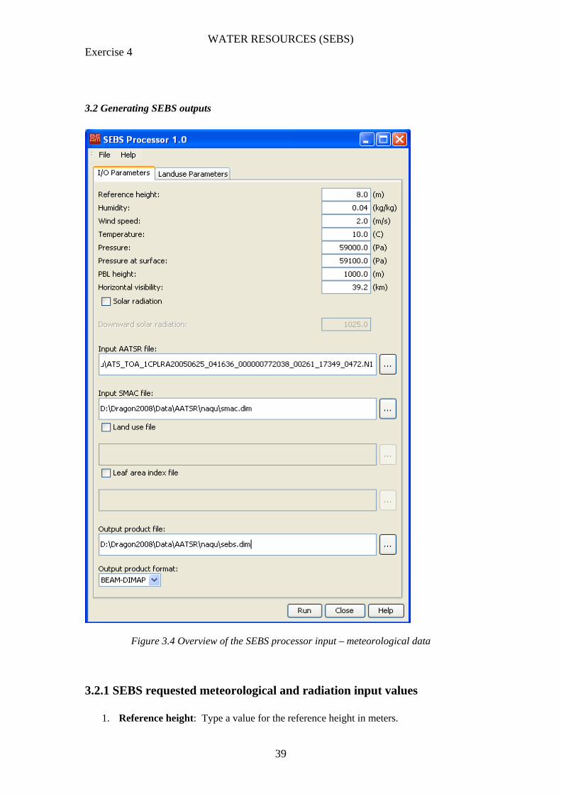
Figure 3.4 Overview of the SEBS processor input – meteorological data

3.2.1 SEBS requested meteorological and radiation input values

1. Reference height: Type a value for the reference height in meters.


40

2. Humidity: Type a value for the specific humidity at reference height in kg per kg.

3. Wind speed: Type a value for the wind speed at reference height in meters per second.

4. Temperature: Type a value for the air temperature at reference height in degree Celsius.

5. Pressure: Type a value for the pressure at reference height in Pa.

6. Pressure at surface: Type a value for the pressure at surface in Pa.

7. Horizontal visibility: Type a value for the horizontal visibility in kilometers.

8. Solar radiation: Select the solar radiation by typing in a value for the downward solar radiation, and run the routine in SEBS (by leaving the solar radiation box unchecked) to calculate the downward radiation value.

3.2.2 SEBS requested satellite input files

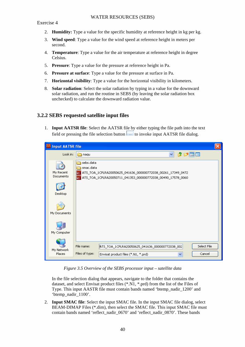
1. Input AATSR file: Select the AATSR file by either typing the file path into the text field or pressing the file selection button to invoke input AATSR file dialog.

Figure 3.5 Overview of the SEBS processor input – satellite data

In the file selection dialog that appears, navigate to the folder that contains the dataset, and select Envisat product files (*.N1, *.prd) from the list of the Files of Type. This input AASTR file must contain bands named ‘btemp_nadir_1200’ and ‘btemp_nadir_1100’.

2. Input SMAC file: Select the input SMAC file. In the input SMAC file dialog, select BEAM-DIMAP Files (*.dim), then select the SMAC file. This input SMAC file must contain bands named ‘reflect_nadir_0670’ and ‘reflect_nadir_0870’. These bands


41

must be atmospherically corrected (use the SMAC processor on the AATSR product in BEAM).

3. Land use file: Select this option if you wish to use land use classes with associated vegetation height values for the estimation of the sensible heat fluxes. This input product must contain a band named ‘land_use_class’. If you select this option, then you are able to define the values of vegetation and roughness height via Landuse Parameters Tab.

4. Leaf area index file: Select this option and select an input file. The input file must contain a band named ‘leaf_area_index’. Unselect this option if you wish to use the routine in SEBS to estimate the leaf area index values.

5. Output product file: Select the SEBS output product file by typing the product path into the text box or by pressing to invoke the file selection button.

6. Output product format: Select the output format (BEAM-DIMAP).

Note that after the successful completion of the SEBS processor, you should see the following bands over the SEBS output file in the BEAM (VISAT) application.

Figure 3.1 Overview of the SEBS processor output

1. sebs_Albodo: Surface albedo 2. sebs_Temperature: Land surface temperature 3. sebs_Rn: Net radiation 4. sebs_G0: Soil heat flux 5. sebs_H_dry: Sensible heat flux at the dry limit 6. sebs_H_wet: Sensible heat flux at the wet limit 7. sebs_H_i: Sensible heat flux 8. sebs_Rel_evap: Evaporative fraction 9. sebs_daily_evap: Actual evaporation on daily base 10. sebs_le : Latent heat flux 11. sebs_emissivity: Surface emissivity 12. sebs_watervapor: Water vapour


42

3.2.3 SEBS Landuse Parameters If you choose to use Land use file in the I/O parameter tab, the Landuse parameter tab appears as the following screen shot:

Figure 3.1 Overview of the SEBS landuse parameters

Vegetation height h (meters): In the first column of the text fields, you are able to change the vegetation height values. The roughness height value in the second column of the text fields is calculated automatically based on the formula used, if the Use Z0m=0.136*h option in the third column is selected. Where z0m is the roughness height of vegetation, and h is the height of vegetation with associated land use class. Roughness height Z0m (meters): This column shows the roughness height values associated to the land use classes. The default value is used, if the Use default Z0m option in the fourth column is selected. Checking the


43

Use Z0m=0.136*h option in the third column lets the Z0m value being calculated using the formula Z0m=0.136*h. Also you are able to define the value of roughness height, if neither Use default Z0m nor Use Z0m=0.136*h is selected. Use Z0m=0.136*h: Checking this option in the third column lets the roughness height value being calculated using the relationship Z0m=0.136*h. The Use default Z0m option in the last column is unchecked automatically, if this option is selected. Use default Z0m: The default value for the roughness height is used, if this option is checked. The Use Z0m=0.136*h option in the last column is unchecked automatically, if this option is selected. Algorithm in SEBS processor (plug-in) SEBS provides a set of methods for retrieval of bio-geophysical parameters: Land surface albedo: The land surface albedo is expressed as a function of the given bands named ‘reflect_nadir_0670’ and ‘reflect_nadir_0870’ from the input SMAC file as:

Albedo = c4 + c5* reflect_nadir_0670/100 + c6 * reflect_nadir_0870/100 Where c4=0.035, c5=0.545, and c6=0.32 are weighting factors. Land surface temperature and emissivity: The spilt-window method for the retrieval of the temperature is implemented in SEBS. The land surface temperature is expressed as a function of the given AATSR bands in nadir views named ‘btemp_nadir_1200’ and ‘btemp_nadir_1100’, and water vapor content. The land surface emissivity is expressed as a function of NDVI. For additional information about the algorithms, refer to Sobrino et al. 2007, AATSR Land-Surface Temperature & Emissivity algorithm theoretical basis document. The water vapor algorithm implemented in SEBS is expressed as a function of the ratio of transmittance estimated from the given AATSR channels in the nadir views (Li et al. 2003. A new approach for retrieving precipitable water from ATSR2 split-window channel data over land area. Int. J. Remote Sens.) Net radiation, Soil heat flux, Sensible heat flux at the dry limit, Sensible heat flux at the wet limit, Actual sensible heat flux, Evaporative fraction, and Actual daily evaporation: You can find the algorithms implemented in Su, 2002, Estimation of the surface energy balance. Hydro. Earth Sys. Sci.

3.3 References

Li, Z.-L., L. Jia, Z. Su, Z. Wan, R.H. Zhang, 2003, A new approach for retrieving precipitable water from ATSR-2 split window channel data over land area, International Journal of Remote Sensing, 24(24), 5095–5117.


44

Rahman, H. and G. Dedieu, 1994, SMAC : a simplified method for the atmospheric correction of satellite measurements in the solar spectrum . Int. J. Remote Sensing, 1994, vol.15, no.1, 123-143.

Sobrino, J.A. and G. Soria, AATSR Land-Surface Temperature & Emissivity, Algorithm Theoretical Basis Document. EU FP6, GMES EAGLE project, SST3-CT2003-502057.

J. A. Sobrino, J. El Kharraz & Z.-L. Li (2003): Surface temperature and water vapour retrieval from MODIS data, International Journal of Remote Sensing, 24:24, 5161-5182

Z. Su, 2002, The Surface Energy Balance System (SEBS) for estimation of turbulent heat fluxes, Hydrology and Earth System Sciences, 6(1), 85-99.

Su, Z., T. Schmugge, W.P. Kustas, W.J. Massman, 2001, An evaluation of two models for estimation of the roughness height for heat transfer between the land surface and the atmosphere, Journal of Applied Meteorology, 40(11), 1933-1951.

Su, Z., 2005, Estimation of the surface energy balance. In: Encyclopedia of hydrological sciences : 5 Volumes. / ed. by M.G. Anderson and J.J. McDonnell. Chichester etc., Wiley & Sons, 2005. 3145 p. ISBN: 0-471-49103-9. Vol. 2 pp. 731-752.

Documents

Practical Session Instructions Earth Observation of Water Resources