Practical Issues with State-Space Models withMixed Stationary and Non-Stationary Dynamics

Technical Paper No. 2010-1

Thomas A. Doan ∗

January 2010

Abstract

State-space models, and the state-space representation of data, are an impor-tant tool for econometric modeling and computation. However, when applied to ob-served (rather than detrended) data, many such models have a mixture of station-ary and non-stationary roots. While Koopman (1997) and Durbin and Koopman(2002) provide “exact” calculations for models with non-stationary roots, thesehave not yet been implemented in most software. Also, neither the Koopman ar-ticle nor the Durbin and Koopman book address (directly) the handling of modelswhere a unit root is shared among several series—a frequent occurrence in state-space models derived from DSGE’s. This paper provides a unified framework forcomputing the finite and “infinite” components of the initial state variance ma-trix which is both flexible enough to handle mixed roots and also faster (even forpurely stationary models) than standard methods. In addition, it examines somespecial problems that arise when the number of unit roots is unknown a priori.

Keywords: Kalman filter, state space methods, non-stationary model

∗Estima, 1560 Sherman Ave #510, Evanston, IL 60201 USA, email:tomd@estima.comThe author thanks participants in seminars at the Bank of England and Cass Business School forhelpful comments, and Tara Sinclair and Ricardo Mestre for providing code and data for their papers.Comments are welcome.

1

1

1 IntroductionState-space models, and the state-space representation of data, are an importanttool for econometric modeling and computation. However, when applied to ob-served (rather than detrended) data, many such models have a mixture of station-ary and non-stationary roots. While Koopman (1997) and Durbin and Koopman(2002) provide “exact” calculations for models with non-stationary roots, thesehave not yet been implemented in most software. Also, neither the Koopmanarticle nor the Durbin and Koopman book address (directly) the handling of mod-els where a unit root is shared among several series—a frequent occurrence instate-space models derived from DSGE’s.

This paper provides a unified framework for computing the finite and “infinite”components of the initial state variance matrix which is both flexible enough tohandle mixed roots and also faster (even for purely stationary models) than stan-dard methods. This is based upon a method for solving for the pre-sample vari-ance which is known in the engineering literature, but largely unknown withineconomics. This is extended to handle non-stationary roots. In addition, it exam-ines some special problems that arise when the number of unit roots is unknowna priori.

The paper is organized as follows. In section 2, we introduce the notation tobe used and describe some common small state-space models, paying particularattention to the types of roots. Section 3 works through a step of the Kalmanfilter with a diffuse prior, showing the differences between an exact treatment ofthe initial conditions and the commonly used approximate handling. Section 4describes other algorithms for computing the initial variances for fully stationarymodels, while section 5 describes a more efficient method based upon the Schurdecomposition of A. Section 6 extends this to non-stationary models. Section 7offer two examples from the literature, highlighting the difference in calculationmethods. Section 8 concludes.

2 State-Space ModelsWe will use the following as our general description of a state-space model:

Xt = AtXt−1 + Zt + Ftwt (1)

Yt = �t + c′tXt + vt (2)

2

{wt,vt} is assumed to be serially independent. Our main focus will be on theproperties of (1), and, in particular, that equation with time-invariant componentmatrices, A, Z, F and Ewtw

′t.

The execution of the Kalman filter requires a pre-sample mean and variance.The ergodic variance is the solution Σ0 to:

AΣ0A′ + Σw = Σ0 (3)

where Σw = F (Ewtw′t) F′. Where this exists, it’s the ideal starting variance since

it is the one initializer that is consistent with the structure of the model. However,it’s well known that there is no solution to (3) if A has roots on the unit circle. Inpractice, the most common way to handle this is use an approximate “diffuse”prior, that is, a pre-sample mean of 0 with a covariance matrix which is a diagonalmatrix with “large” numbers. While not completely unreasonable, there are anumber of numerical problems with this approach, particularly if the estimates ofstate variances are of interest.

In the Unobserved Components (UC) models analyzed extensively in Harvey(1989), the A matrices have all unit roots: the local level model has a single unitroot, the local trend has a double (repeated) unit root, and the seasonal modelshave S− 1 seasonal roots of 1 (other than 1 itself). The state-space representationapplied to ARMA models, on the other hand, has all roots inside the unit circle inorder to permit the calculation of the full sample likelihood—the non-stationarityof the ARIMA model is typically handled by differencing the data and applyingthe state-space techniques to that.

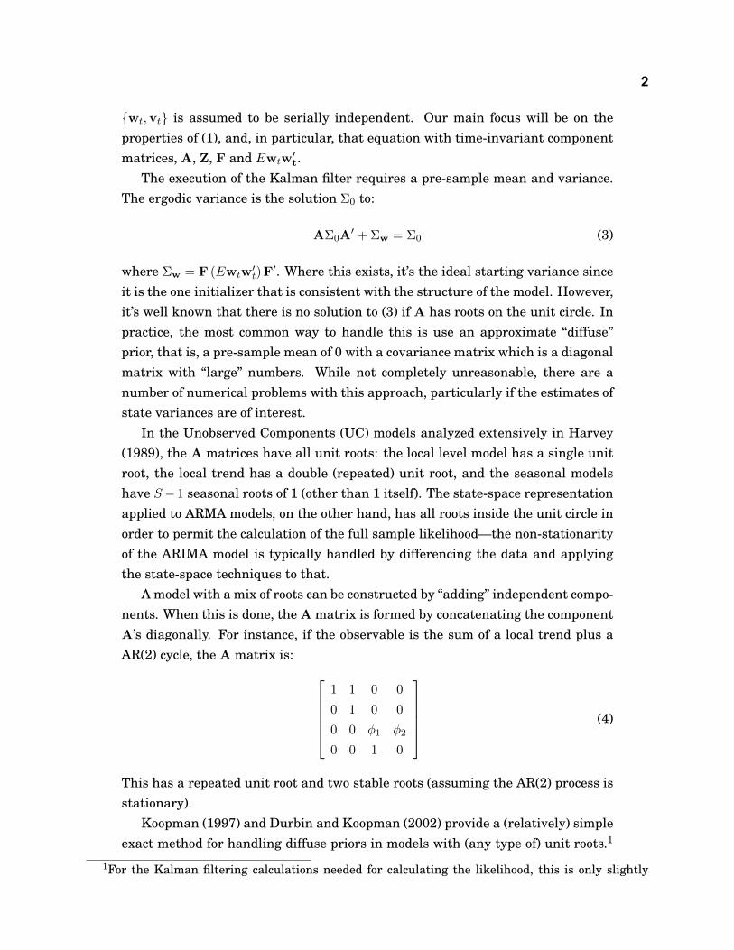
A model with a mix of roots can be constructed by “adding” independent compo-nents. When this is done, the A matrix is formed by concatenating the componentA’s diagonally. For instance, if the observable is the sum of a local trend plus aAR(2) cycle, the A matrix is: ⎡⎢⎢⎢⎢⎣

1 1 0 0

0 1 0 0

0 0 �1 �2

0 0 1 0

⎤⎥⎥⎥⎥⎦ (4)

This has a repeated unit root and two stable roots (assuming the AR(2) process isstationary).

Koopman (1997) and Durbin and Koopman (2002) provide a (relatively) simpleexact method for handling diffuse priors in models with (any type of) unit roots.1

1For the Kalman filtering calculations needed for calculating the likelihood, this is only slightly

3

The Durbin-Koopman textbook also describes a way of handling a mixture of unitand stationary roots, but offers little guidance as to how to handle this in any sit-uation where the states don’t partition nicely as in (4). For instance, their descrip-tion of the non-stationary ARIMA model uses yt,Δyt,Δyt−1, ... as the states ratherthan yt, yt−1, yt−2, .... However, this type of transformation isn’t always practical—in some cases, the state-space model is derived from a more complicated problem,and the precise positioning of states may not be well known to the user.2

The method proposed in this paper uses the properties of the A and ΣW ma-trices only (thus not requiring any ingenuity on the part of the user) to derive apartially diffuse, partially stationary initialization.

3 Diffuse PriorIn practical state-space models, it’s rare for all the eigenvalues of the transitionmatrix to be inside the unit circle. In the simplest of the non-stationary models,the local level model, the “solution” for (3) is var(X) = ∞. Suppose that we use aprior of mean 0 and variance � where � is “large”. The Kalman updating equationfor the mean is

x1∣1 = x1∣0 +�21∣0

�21∣0 + �2v

(y1 − x1∣0

)With �21∣0 = �+ �2w, if � is large relative to �2w and �2v this will be approximated by

x1∣1 = x1∣0 + 1.0(y1 − x1∣0

)or x1∣1 = y1. This shouldn’t come as a surprise; with a very high prior variance,the data will dominate completely. The only data information after one data pointis that one value. This calculation isn’t particularly sensitive to the precise valueof � as long as it’s big enough.

The variance calculation is more problematical. The calculation (in practice) isdone by:

�21∣1 = �21∣0 −

(�21∣0

)2�21∣0 + �2v

While we can rearrange this (algebraically) to give �21∣1 ≈ �2v , the calculation willbe done in software as the subtraction above. Subtracting two very large and

more complicated than the standard Kalman filter. Kalman smoothing isn’t quite as straightforward,and is, in fact, described incorrectly in the Koopman article.

2For instance, to produce the state-space representation for a model with expectational terms, thestate vector can require augmentation with lags, with the number depending upon the precise form ofeach equation in the model.

4

almost equal numbers to produce a small number runs the danger of a completeloss of precision. With the standard 15 digit precision on a modern computer, if �is greater than 1015�2v , the calculation above will give zero.

So in order for this to give us the desired results by using large values of �, weneed to choose a value which is large enough, but not too large. For this model,we can probably figure out a way to do that. With a more complicated model withmultiple variances, some of which might be quite small, we’re less likely to findsuch a value.

Note, by the way, that one suggested strategy is to try several values for �,and check for sensitivity.3 While better than just picking an arbitrary number,looking for sensitivity on estimates of the mean will likely overlook the more trou-blesome calculation of the variance. And the calculation that is most affected byapproximation error is the state variance for Kalman smoothing. Those are highlysuspect in any calculation done this way.4

This calculation is effectively identical if the model is, in fact, stationary, buta diffuse prior is being used for convenience. If, instead of the random walk, theunderlying state equation is xt = �xt−1 + wt with ∣�∣ < 1, then we still will getx1∣1 ≈ y1 and �1∣1 ≈ �2v . This is not the same as what we would get if we used theergodic variance, but isn’t necessarily an unreasonable procedure.5

An alternative to approximating this was provided by Koopman (1997), whichis exact diffuse initialization. This was later refined in Durbin and Koopman(2002). This is done by doing the actual limits as � → ∞. It is implementedby writing covariance matrices in the form Σ∞� + Σ∗ where Σ∞ is the “infinite”part and Σ∗ is the “finite” part. These are updated separately as needed.

This works in the following way for the local level model. The prior is mean0. The prior covariance is [1]� + [0].6 Moving to �1∣0 adds the finite �2w, producing[1]�+ [�2w]. The predictive variance for y1 further adds �2v , to make [1]�+ [�2w + �2v ].The Kalman gain is the multiplier on the prediction error used in updating thestate. That’s (

[1]�+ [�2w]) (

[1]�+ [�2w + �2v ])−1 (5)

Inverses can be computed by matching terms in a power series expansion in �−1

3For instance, Koopman, Shepard, and Doornik (1999) suggest calculating once with an standard“large” value, then recalculating with a revised value based upon the initial results.

4In a model with more than one diffuse state, the filtered covariance matrix after a small numberof data points will still have some very large values. Those are only reduced to “finite” numbers as theresult of the smoothing calculation, which uses information obtained by calculating out to the end ofthe data set and back, accumulating roundoff error along the way.

5With the ergodic variance, x1∣1 will be a weighted average of 0 and y1 with weights equal to theergodic variance and �2

v respectively.6We’ll keep the different components in brackets.

5

as shown in Appendix A. For computing the mean, all we need are the 1 and �−1

terms, which allows us to write (5) as approximately:

([1]�+ [�2w]

) ([0] + [1]�−1

)= [1] + [�2w]�−1

where the approximation in the inverse will produce only an additional term onthe order of �−2. We can now pass to the limit (that is, ignore all but the finiteterm) and get the Kalman gain as 1 (exactly), as we expected.

Getting the filtered variance correct requires greater accuracy. For that, we’llneed to expand the inverse to the �−2 level. We need this because the updatingequation is:

([1]�+ [�2w]

)−([1]�+ [�2w]

) ([1]�+ [�2w + �2v ]

)−1 ([1]�+ [�2w]

)and the inverse is sandwiched between two factors, each with a �. As a result,terms in �−2 in the inverse will produce a finite value when this is multipliedout, and only �−3 and above will be negligible. The second order expansion of therequired inverse is (

[0] + [1]�−1 − [�2w + �2v ]�−2)

The calculation of the filtered variance is most conveniently done as(1−

([1]�+ [�2w]

) ([1]�+ [�2w + �2v ]

)−1) ([1]�+ [�2w]

)(6)

With the second order expansion, the product

([1]�+ [�2w]

) ([1]�+ [�2w + �2v ]

)−1produces

1− �2v�−1 −O(�−2) (7)

Plugging that into (6) results in �2v + O(�−1). Passing to the limit gives us theresult we want.

Note that the calculation here that causes the problem for large, but finitevalues, is subtracting (7) from 1. If we have a loss of precision there, we won’t get�2v out; we’ll get zero.

While we started with an “infinite” variance, after seeing one data point, wenow have x1∣1 = y1 , �1∣1 = �2v , which are perfectly reasonable finite values. We canKalman filter in the standard fashion from there.

6

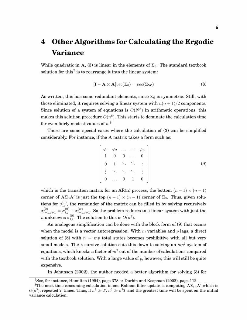
4 Other Algorithms for Calculating the ErgodicVariance

While quadratic in A, (3) is linear in the elements of Σ0. The standard textbooksolution for this7 is to rearrange it into the linear system:

[I−A⊗A]vec(Σ0) = vec(ΣW) (8)

As written, this has some redundant elements, since Σ0 is symmetric. Still, withthose eliminated, it requires solving a linear system with n(n+ 1)/2 components.Since solution of a system of equations is O(N3) in arithmetic operations, thismakes this solution procedure O(n6). This starts to dominate the calculation timefor even fairly modest values of n.8

There are some special cases where the calculation of (3) can be simplifiedconsiderably. For instance, if the A matrix takes a form such as:⎡⎢⎢⎢⎢⎢⎢⎢⎢⎣

'1 '2 . . . . . . 'n

1 0 0 . . . 0

0 1. . . . . . ...

... . . . . . . . . . ...0 . . . 0 1 0

⎤⎥⎥⎥⎥⎥⎥⎥⎥⎦(9)

which is the transition matrix for an AR(n) process, the bottom (n− 1) × (n− 1)

corner of AΣ0A′ is just the top (n− 1) × (n− 1) corner of Σ0. Thus, given solu-

tions for �(0)1j , the remainder of the matrix can be filled in by solving recursively�(0)i+1,j+1 = �

(0)i,j + �

(w)i+1,j+1. So the problem reduces to a linear system with just the

n unknowns �(0)1j . The solution to this is O(n3).An analogous simplification can be done with the block form of (9) that occurs

when the model is a vector autoregression. With m variables and p lags, a directsolution of (8) with n = mp total states becomes prohibitive with all but verysmall models. The recursive solution cuts this down to solving an mp2 system ofequations, which knocks a factor of m2 out of the number of calculations comparedwith the textbook solution. With a large value of p, however, this will still be quiteexpensive.

In Johansen (2002), the author needed a better algorithm for solving (3) for

7See, for instance, Hamilton (1994), page 378 or Durbin and Koopman (2002), page 112.8The most time-consuming calculation in one Kalman filter update is computing AΣt∣tA

′ which isO(n3), repeated T times. Thus, if n3 ≫ T , n6 ≫ n3T and the greatest time will be spent on the initialvariance calculation.

7

precisely this reason—the corrections needed the ergodic solution for a state-space representation for a VAR. His proposal was to transform (3) by taking amatrix P such that PAP−1 = Λ and PΣwP−1 = D, where Λ and D are diagonal.Pre-multiplying (3) by P and post-multiplying by P−1 and inserting P−1P in twoplaces produces the equation:

PAP−1PΣ0P−1PA′P

−1+ PΣwP−1 = PΣ0P

−1 (10)

Defining Σp = PΣ0P−1 and substituting the reductions for A and Σw gives us:

ΛΣpΛ + D = Σp

Because Λ is diagonal, this reduces to the set of equations:

�(p)ij �i�j = dij + �

(p)ij (11)

Thus, we can directly compute �(p)ij , which will also be a diagonal matrix (since D

is diagonal) and then can recover the desired matrix with Σ0 = P−1ΣpP. Becausefinding eigenvalues and vectors of an n × n matrix is an O(n3) calculation, thisreduces the burden by a factor of O(n3).9

One thing to note is that the requirement that P be a joint diagonalizing matrixisn’t really necessary. The solution for (11) is very simple whether PΣwP−1 = D

is diagonal or not. One complication with this (depending upon the software used)is that, in general, P and Λ will be complex matrices, and Σp will be Hermitianrather than symmetric. Allowing for complex roots, the �j in (11) needs to beconjugated.

A more serious problem is that not all state matrices will be diagonalizable.Although it’s a case with unit roots (which will be covered later), the standardlocal trend model transition matrix [

1 1

0 1

]

isn’t diagonalizable, and, in fact, is already in its Jordan form. State-space modelssolved out of DSGE’s also frequently have repeated eigenvalues.

9Because the final step in computing eigenvalues is iterative, the computational complexity isn’tprecisely known. The O(n3) is based upon a fixed number of iterations per eigenvalue.

8

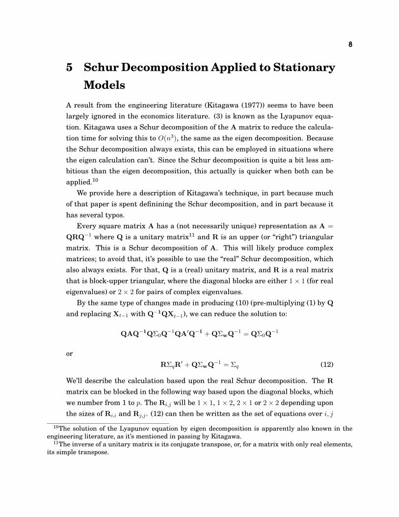
5 Schur Decomposition Applied to StationaryModels

A result from the engineering literature (Kitagawa (1977)) seems to have beenlargely ignored in the economics literature. (3) is known as the Lyapunov equa-tion. Kitagawa uses a Schur decomposition of the A matrix to reduce the calcula-tion time for solving this to O(n3), the same as the eigen decomposition. Becausethe Schur decomposition always exists, this can be employed in situations wherethe eigen calculation can’t. Since the Schur decomposition is quite a bit less am-bitious than the eigen decomposition, this actually is quicker when both can beapplied.10

We provide here a description of Kitagawa’s technique, in part because muchof that paper is spent definining the Schur decomposition, and in part because ithas several typos.

Every square matrix A has a (not necessarily unique) representation as A =

QRQ−1 where Q is a unitary matrix11 and R is an upper (or “right”) triangularmatrix. This is a Schur decomposition of A. This will likely produce complexmatrices; to avoid that, it’s possible to use the “real” Schur decomposition, whichalso always exists. For that, Q is a (real) unitary matrix, and R is a real matrixthat is block-upper triangular, where the diagonal blocks are either 1× 1 (for realeigenvalues) or 2× 2 for pairs of complex eigenvalues.

By the same type of changes made in producing (10) (pre-multiplying (1) by Q

and replacing Xt−1 with Q−1QXt−1), we can reduce the solution to:

QAQ−1QΣ0Q−1QA′Q−1 + QΣwQ−1 = QΣ0Q

−1

orRΣqR

′ + QΣwQ−1 = Σq (12)

We’ll describe the calculation based upon the real Schur decomposition. The R

matrix can be blocked in the following way based upon the diagonal blocks, whichwe number from 1 to p. The Ri,j will be 1× 1, 1× 2, 2× 1 or 2× 2 depending uponthe sizes of Ri,i and Rj,j . (12) can then be written as the set of equations over i, j

10The solution of the Lyapunov equation by eigen decomposition is apparently also known in theengineering literature, as it’s mentioned in passing by Kitagawa.

11The inverse of a unitary matrix is its conjugate transpose, or, for a matrix with only real elements,its simple transpose.

9

combinations of:

p∑l=i

Ri,l

⎧⎨⎩p∑

m=j

Σ(q)l,m (Rj,m)′

⎫⎬⎭+ Wi,j = Σ(q)i,j (13)

which uses the block triangularity of R in the lower limits on the two sums.12 Thiscan be solved recursively starting with i = j = p, which is:

Rp,pΣ(q)p,pRp,p + Wp,p = Σ(q)

p,p

This takes the form of a Lyapunov equation, but with matrices that are at most2×2, so the textbook solution method can be employed. Solving (13) at i, j requiresΣ(∗)l,m for all combinations with m > j or m = j and l > i. Thus the solution order

is to work up column p, then solve for p− 1, p− 1, then work up column p− 1, etc.The largest system that needs to be solved is a standard linear system with fourunknowns for the off-diagonal 2× 2.

Done literally, (13) is an O(n4) calculation, since for each of the O(n2) combi-nations i, j the double sum of terms to the right or below is O(n2). However, theterm in braces can be computed just once for each l in column j.13 Each of thosesums is O(n), done n times (over l) and n times (over j), thus O(n3). However,they produce small matrices14, so the sum over l is O(n), done O(n2) times overi, j, again giving the desired O(n3).

The final step is to transform back to the original space with Σ0 = Q′ΣqQ,which is, itself, an O(n3) calculation.

Table 1 gives a comparison of the Schur and eigen methods with the textbookcalculation for various numbers of states. These are in number of calculationsper second, and show the rapid deterioration of speed with size for the standardcalculation.15

6 Generalized Ergodic InitializationThe extension to non-stationary models is straightforward. Appendix B showsthat the estimated means and variances of the states aren’t dependent upon the

12Note that Σ(q)i,j appears in a term in the double sum, which will have to be pulled out when solving.

13When we start on column j, we don’t yet know Σ(∗)l,j for l ⩽ j. So the terms involving those are

initially omitted and are added into term l once we’ve solved l, j.14Depending upon the sizes of the blocks, each is a 1× 1, 1× 2, 2× 1 or 2× 2 matrix.15These were done on a 2GHz Dell Laptop running Windows Vista. The standard method was solved

using LU decomposition.

10

Table 1: Speed Comparison

n Schur Eigen Standard10 4464.3 1976.3 847.520 961.5 339.0 24.630 250.0 101.0 2.550 31.3 22.5 .1

100 4.3 3.2

precise form of the diffuse prior, so we will choose an identity matrix in the Q

transformed representation.The solutions for the diagonal blocks in (13) will be in the general form of a

Lyapunov equation. If Rj,j has unit eigenvalues, then there is no solution. If theeigenvalues are outside the unit circle, there will generally be a solution, but it isunlikely to be useful in economic applications, so we treat them the same as theunit roots.16 Classify the diagonal blocks as stationary or non-stationary. MakeΣ(q)i,j = 0 for any block where either i or j is a non-stationary block and otherwise

solve (13) as described in the previous section. In a parallel “diffuse matrix”, makeΣ(∞)i,j = I if i = j and i is a non-stationary block and make it zero otherwise. Note

that, if the blocks were ordered so the non-stationary roots were at the lowerright, this would have Σq blocked with non-zeros only in the top left and Σ∞ beingblocked with an identity matrix in the lower right. Since sorting the eigenvaluesin the Schur decomposition is a complicated and time-consuming task, doing theequivalent calculation while leaving them in the order in which they’re originallyproduced is the best strategy.

The finite and infinite components in the original representation are then pro-duced by back transforming by the Q matrix as before. The result of this we willcall the Generalized Ergodic Initialization for the model. Note that it isn’t uniquesince there are many equivalent choices for the diffuse component.

Because of the possibility of round-off error, the test for unit eigenvalues hasto allow for some flexibility, that is, the test needs to be whether the roots are big-ger than something like .9999999. There are some practical problems which arisewhen a model has near unit roots, or roots that might, or might not be unit. Oneof these problems is that there’s no continuous definition of the likelihood functionwhen you move from a near unit root to a unit root. The standard recursive defini-tion of the likelihood is based upon the predictive density for the observable. Witha large, but finite, variance, that likelihood element is computable, although the

16Kitagawa allows for explosive roots, and, in fact, his example includes some.

11

log likelihood element will be a large negative number. If the predictive varianceis infinite, the likelihood is, theoretically, zero and thus the log likelihood isn’tdefined.

The only way to handle this is to use the conditional rather than uncondi-tional likelihood. That’s done automatically in case a unit root is detected. For astate-space model, the conditional likelihood is calculated by not including a cer-tain number of early data points. The number of data points skipped needs to beat least large enough so that the observables cover the possible number of unitroots.17

The other problem is that the calculation is also discontinuous due to the shiftin algorithm once a root gets inside the zone where we treat it as a unit root. We’vefound this to be the more vexing of the two problems. The discontinuity itself isn’tas significant a problem as the lack of (true) differentiability that it implies. Thearc derivatives, which should converge to the computed directional derivatives,don’t. As a result, standard procedures for selecting a step size in hill-climbingmethods like BFGS or BHHH will fail to work properly.

In order to finesse this, we have found that the simplest solution was to useconditional likelihood with a fully diffuse prior for a certain number of iterationsin order to get the estimates relatively close to the proper range. At that point,we switched over to the correctly computed variance. While the fully diffuse priorisn’t really correct, it’s close enough to use as an improvement on the initial guessvalues for the parameters.

7 ExamplesWe now look at two examples where approximate and fully diffuse priors wereused and see how the calculations are affected by different ways of handling theinitial conditions. These were not chosen as particularly extreme examples—thereare just examples with more than one observable, state models with combinationsof stationary and non-stationary roots for which the estimating code has beengraciously made available, so the precise calculations used can be reproduced.

17If there is only one observable, this would mean if there are r potential unit roots, one shouldcondition on r data points. If there is more than one observable, it could be fewer. In most cases, aslong as the number of observables times the number of conditioning data points is at least as large asr, the likelihood will be consistently defined.

12

7.1 Example 1Sinclair (2009) estimates a bivariate time series model with US log GDP and un-employment rate as the observables. Each series is modeled with a local trendwith fixed growth plus an AR(2) cycle.

Xt =

⎡⎢⎢⎢⎢⎢⎢⎢⎢⎢⎣

1 0 0 0 0 0

0 �y1 �y2 0 0 0

0 1 0 0 0 0

0 0 0 1 0 0

0 0 0 0 �u1 �u2

0 0 0 0 1 0

⎤⎥⎥⎥⎥⎥⎥⎥⎥⎥⎦Xt−1 +

⎡⎢⎢⎢⎢⎢⎢⎢⎢⎢⎣

�y

0

0

�u

0

0

⎤⎥⎥⎥⎥⎥⎥⎥⎥⎥⎦+

⎡⎢⎢⎢⎢⎢⎢⎢⎢⎢⎣

1 0 0 0

0 1 0 0

0 0 0 0

0 0 1 0

0 0 0 1

0 0 0 0

⎤⎥⎥⎥⎥⎥⎥⎥⎥⎥⎦

⎡⎢⎢⎢⎢⎣wy1t

wy2t

wu1t

wu2t

⎤⎥⎥⎥⎥⎦

Yt =

[1 1 0 0 0 0

0 0 0 1 1 0

]Xt

This has two unit roots among six states, and has four shocks (there are nomeasurement errors). We look at her model without the break. Sinclair’s han-dling was to use an approximate diffuse prior with 107 diagonal elements, withestimates computed conditioning on four data points to avoid problems with apoorly defined likelihood for those initial values. (With six diffuse states and twoequations, this could safely be done conditioning on just three data points.) Table2 shows the smoothed state and variance estimates at t = 1, t = 4 and t = 10

with the approximate fully diffuse prior, with an approximate diffuse prior with108 rather than 107, an exact fully diffuse prior and the mixed ergodic prior.

As we can see from this, the approximate diffuse priors do a good job of comput-ing the smoothed mean at t = 1, but the variance calculation is quite sensitive. Inthis case, 107 is already a bit too large—106 (not shown) produces a similar resultto the exact diffuse prior.

Table 3 compares the maximum likelihood estimates done four ways. The firstthree use the same conditioning on four data points as in the paper. The firstcolumn is the approximate diffuse prior as in the paper, the second is the exactfully diffuse prior and the third uses the mixed ergodic initialization. The finalcolumn does the mixed ergodic calculation conditioning on the minimal amountof information. The first five rows have the AR coefficients and the mean growthrate for y. (The mean growth rate of u is pegged at zero). The covariance matrixof the shocks is estimated in Choleski factor form. As we can see, the effect ofapproximating the diffuse prior is negligible. In this case, the loss of data byexcess conditioning seems (comparing third and fourth columns) to be less of a

13

Table 2: Sinclair ModelGDP Trend GDP Cycle UR Trend UR Cycle

Time=1107 Diffuse 739.824 −1.049 3.770 −0.070

1.761 1.761 0.337 0.337108 Diffuse 739.824 −1.049 3.770 −0.070

1.768 1.819 0.880 1.008Exact Diffuse 739.824 −1.049 3.770 −0.070

1.761 1.761 0.325 0.325Ergodic 738.727 0.048 3.880 −0.180

0.365 0.365 0.105 0.105

Time=4107 Diffuse 738.421 2.915 5.676 −1.876

0.328 0.328 0.094 0.094108 Diffuse 738.421 2.915 5.676 −1.876

0.328 0.328 0.094 0.094Exact Diffuse 738.421 2.915 5.676 −1.876

0.328 0.328 0.094 0.094Ergodic 738.520 2.816 5.648 −1.848

0.301 0.301 0.093 0.093

Time=10107 Diffuse 748.549 −1.965 4.150 1.450

0.300 0.300 0.093 0.093108 Diffuse 748.549 −1.965 4.150 1.450

0.300 0.300 0.093 0.093Exact Diffuse 748.549 −1.965 4.150 1.450

0.300 0.300 0.093 0.093Ergodic 748.541 −1.958 4.150 1.450

0.300 0.300 0.093 0.093

14

factor than using a fully diffuse prior (comparing second and third); since theAR(2) cycles have fairly small roots, that’s probably not unexpected.

Table 3: Sinclair EstimatesApprox Diffuse Exact Diffuse Conditional Ergodic Full Ergodic

�y1 0.743 0.743 0.744 0.747�y2 −0.266 −0.266 −0.289 −0.293�y 0.842 0.842 0.845 0.846�u1 0.697 0.697 0.672 0.669�u2 −0.174 −0.174 −0.174 −0.175F11 1.453 1.453 1.427 1.410F21 −0.824 −0.824 −0.780 −0.763F22 0.496 0.496 0.478 0.475F31 −0.643 −0.643 −0.637 −0.629F32 0.068 0.068 0.033 0.028F33 0.238 0.238 0.254 0.253F41 0.607 0.607 0.585 0.575F42 −0.189 −0.189 −0.156 −0.151F43 −0.114 −0.114 −0.121 −0.121F44 −0.000 −0.000 0.000 −0.000

7.2 Example 2The “baseline” system in Fabiani and Mestre (2004) has three observables: log ofGDP, unemployment rate and inflation rate. The state equation takes the form:

⎡⎢⎢⎢⎢⎢⎢⎢⎢⎢⎢⎢⎢⎢⎢⎣

y∗t

�t

(y − y∗)t(y − y∗)t−1

u∗t

�t

(u− u∗)t(u− u∗)t−1

⎤⎥⎥⎥⎥⎥⎥⎥⎥⎥⎥⎥⎥⎥⎥⎦=

⎡⎢⎢⎢⎢⎢⎢⎢⎢⎢⎢⎢⎢⎢⎢⎣

1 1 0 0 0 0 0 0

0 1 0 0 0 0 0 0

0 0 0 0 0 0 �1 0

0 0 1 0 0 0 0 0

0 0 0 0 1 1 0 0

0 0 0 0 0 1 0 0

0 0 0 0 0 0 �1 �2

0 0 0 0 0 0 1 0

⎤⎥⎥⎥⎥⎥⎥⎥⎥⎥⎥⎥⎥⎥⎥⎦Xt−1+

⎡⎢⎢⎢⎢⎢⎢⎢⎢⎢⎢⎢⎢⎢⎢⎣

1 0 0 0 0 0

0 1 0 0 0 0

0 0 1 0 0 0

0 0 0 0 0 0

0 0 0 1 0 0

0 0 0 0 1 0

0 0 0 0 0 1

0 0 0 0 0 0

⎤⎥⎥⎥⎥⎥⎥⎥⎥⎥⎥⎥⎥⎥⎥⎦

⎡⎢⎢⎢⎢⎢⎢⎢⎢⎢⎣

"y∗t

"�t

"yct

"u∗t

"�t

"uct

⎤⎥⎥⎥⎥⎥⎥⎥⎥⎥⎦

where y∗t is potential GDP, modeled as a local trend, u∗t is the NAIRU, also mod-eled as a local trend, (y − y∗)t and (u− u∗)t are the output and unemploymentgaps, respectively. The unemployment gap is modeled as an AR(2) process, whilethe output gap depends upon the lagged unemployment gap. Observed GDP is

15

the sum (without error) of the latent y∗t and (y − y∗)t; similarly for observed un-employment. Observed inflation is modeled largely as a regression equation onlags of itself and lagged inflation in imports, with a loading from the lagged un-employment gap as the connection with the state space model. This has four unitroots (two sets of repeated roots) among eight states, with seven shocks: six in thestate equation, plus a measurement error in the inflation equation.

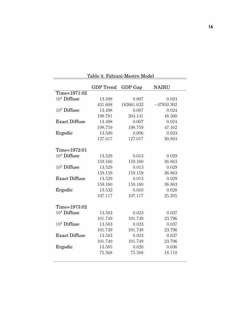
The variances are quite small, so the approximate diffuse prior used in thepaper was 104 variances, and the likelihood function was computed conditionalon eight data points. Again, this is quite a bit more than is actually required,since with three observables, only three observations are needed to cover the eightstates. As with the previous example, the smoothed means and variances areshown for observations 1, 4 and 10; because of the small scales of the variances,they are all multiplied by 106. For t = 1, the smoothed variance computed usingthe paper’s approximation shows a rather catastrophic loss of precision. We alsoshow this calculated with 102 initial variances, which is better behaved. Again,the mean isn’t sensitive to the choice between these.

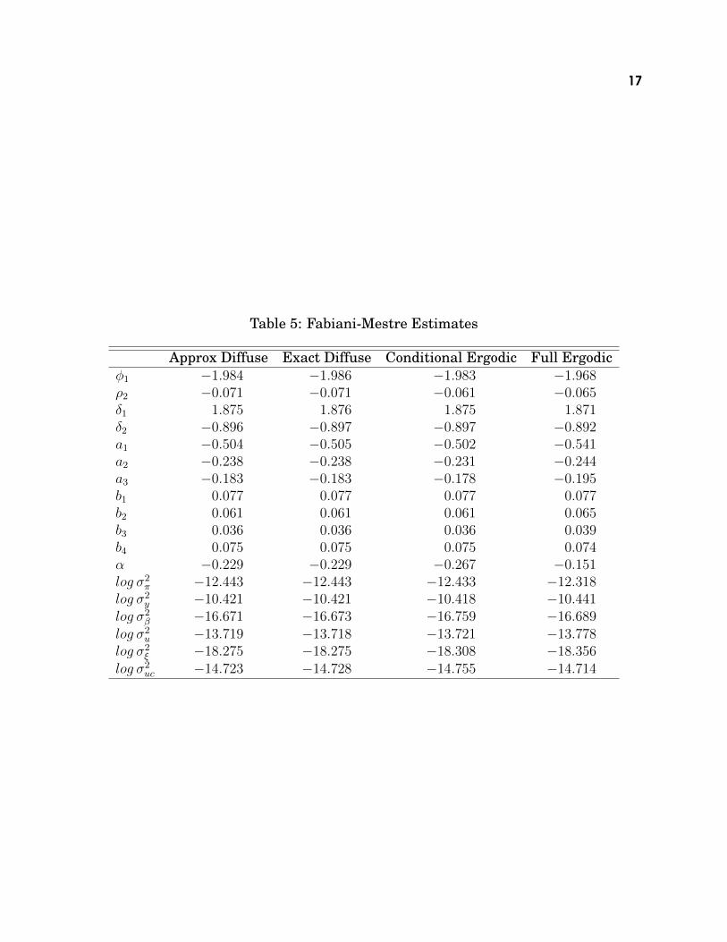
Table 7.2 shows a comparison of estimates, similar to what was done in the firstexample. The ai, bi and � are the regression coefficients from the inflation equationand �2 is the loading for the unemployment gap on inflation. In this case, the lossof data points seems to be much more of an issue, probably because it’s now fiverather than one, and also because the AR(2) process for the unemployment gaphas two fairly large roots, so the fully diffuse prior isn’t as far off as it might be inother applications.

8 ConclusionThis paper has re-introduced and extended a result from the engineering liter-ature for computing the initial variance for state-space models with a mixtureof stationary and non-stationary roots. In addition to being capable of handlingnon-stationary states, it is also faster than the “textbook” method even for fullystationary models. We have also used empirical examples to document the possi-ble problems with the use of simpler techniques for approximating diffuse priors.

16

Table 4: Fabiani-Mestre Model

GDP Trend GDP Gap NAIRUTime=1971:02104 Diffuse 13.498 0.007 0.024

431.608 182661.632 −47950.302102 Diffuse 13.498 0.007 0.024

198.781 204.141 48.560Exact Diffuse 13.498 0.007 0.024

198.759 198.759 47.162Ergodic 13.500 0.006 0.023

127.017 127.017 30.804

Time=1972:01104 Diffuse 13.529 0.013 0.029

159.160 159.160 36.863102 Diffuse 13.529 0.013 0.029

159.159 159.159 36.863Exact Diffuse 13.529 0.013 0.029

159.160 159.160 36.863Ergodic 13.532 0.010 0.028

107.117 107.117 25.205

Time=1973:02104 Diffuse 13.583 0.023 0.037

101.749 101.749 23.796102 Diffuse 13.583 0.023 0.037

101.749 101.749 23.796Exact Diffuse 13.583 0.023 0.037

101.749 101.749 23.796Ergodic 13.585 0.020 0.036

75.568 75.568 18.110

17

Table 5: Fabiani-Mestre Estimates

Approx Diffuse Exact Diffuse Conditional Ergodic Full Ergodic�1 −1.984 −1.986 −1.983 −1.968�2 −0.071 −0.071 −0.061 −0.065�1 1.875 1.876 1.875 1.871�2 −0.896 −0.897 −0.897 −0.892a1 −0.504 −0.505 −0.502 −0.541a2 −0.238 −0.238 −0.231 −0.244a3 −0.183 −0.183 −0.178 −0.195b1 0.077 0.077 0.077 0.077b2 0.061 0.061 0.061 0.065b3 0.036 0.036 0.036 0.039b4 0.075 0.075 0.075 0.074� −0.229 −0.229 −0.267 −0.151log �2

� −12.443 −12.443 −12.433 −12.318log �2

y −10.421 −10.421 −10.418 −10.441log �2

� −16.671 −16.673 −16.759 −16.689log �2

u −13.719 −13.718 −13.721 −13.778log �2

� −18.275 −18.275 −18.308 −18.356log �2

uc −14.723 −14.728 −14.755 −14.714

18

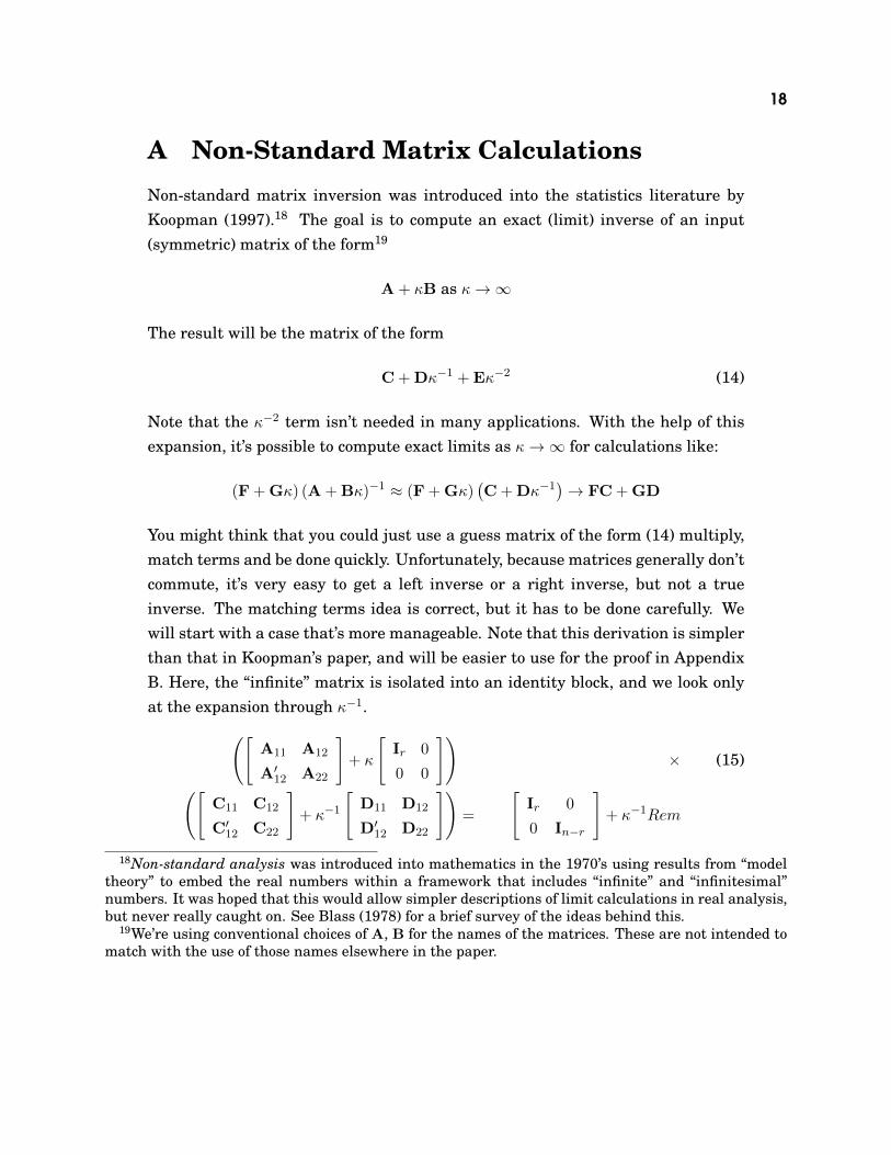
A Non-Standard Matrix CalculationsNon-standard matrix inversion was introduced into the statistics literature byKoopman (1997).18 The goal is to compute an exact (limit) inverse of an input(symmetric) matrix of the form19

A + �B as �→∞

The result will be the matrix of the form

C + D�−1 + E�−2 (14)

Note that the �−2 term isn’t needed in many applications. With the help of thisexpansion, it’s possible to compute exact limits as �→∞ for calculations like:

(F + G�) (A + B�)−1 ≈ (F + G�)(C + D�−1

)→ FC + GD

You might think that you could just use a guess matrix of the form (14) multiply,match terms and be done quickly. Unfortunately, because matrices generally don’tcommute, it’s very easy to get a left inverse or a right inverse, but not a trueinverse. The matching terms idea is correct, but it has to be done carefully. Wewill start with a case that’s more manageable. Note that this derivation is simplerthan that in Koopman’s paper, and will be easier to use for the proof in AppendixB. Here, the “infinite” matrix is isolated into an identity block, and we look onlyat the expansion through �−1.([

A11 A12

A′12 A22

]+ �

[Ir 0

0 0

])× (15)([

C11 C12

C′12 C22

]+ �−1

[D11 D12

D′12 D22

])=

[Ir 0

0 In−r

]+ �−1Rem

18Non-standard analysis was introduced into mathematics in the 1970’s using results from “modeltheory” to embed the real numbers within a framework that includes “infinite” and “infinitesimal”numbers. It was hoped that this would allow simpler descriptions of limit calculations in real analysis,but never really caught on. See Blass (1978) for a brief survey of the ideas behind this.

19We’re using conventional choices of A, B for the names of the matrices. These are not intended tomatch with the use of those names elsewhere in the paper.

19

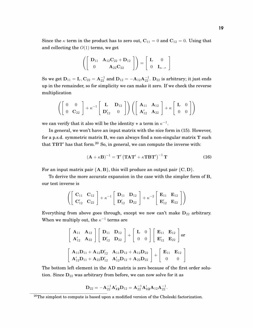
Since the � term in the product has to zero out, C11 = 0 and C12 = 0. Using thatand collecting the O(1) terms, we get([

D11 A12C22 + D12

0 A22C22

])=

[Ir 0

0 In−r

]

So we get D11 = Ir,C22 = A−122 and D12 = −A12A−122 . D22 is arbitrary; it just ends

up in the remainder, so for simplicity we can make it zero. If we check the reversemultiplication([

0 0

0 C22

]+ �−1

[Ir D12

D′12 0

])([A11 A12

A′12 A22

]+ �

[Ir 0

0 0

])

we can verify that it also will be the identity + a term in �−1.In general, we won’t have an input matrix with the nice form in (15). However,

for a p.s.d. symmetric matrix B, we can always find a non-singular matrix T suchthat TBT′ has that form.20 So, in general, we can compute the inverse with:

(A + �B)−1 = T′(TAT′ + �TBT′

)−1T (16)

For an input matrix pair {A,B}, this will produce an output pair {C,D}.To derive the more accurate expansion in the case with the simpler form of B,

our test inverse is([C11 C12

C′12 C22

]+ �−1

[D11 D12

D′12 D22

]+ �−2

[E11 E12

E′12 E22

])

Everything from above goes through, except we now can’t make D22 arbitrary.When we multiply out, the �−1 terms are[

A11 A12

A′12 A22

][D11 D12

D′12 D22

]+

[Ir 0

0 0

][E11 E12

E′12 E22

]or

[A11D11 + A12D

′12 A11D12 + A12D22

A′12D11 + A22D′12 A′12D12 + A22D22

]+

[E11 E12

0 0

]The bottom left element in the AD matrix is zero because of the first order solu-tion. Since D22 was arbitrary from before, we can now solve for it as

D22 = −A−122 A′12D12 = A−122 A′12A12A−122 .

20The simplest to compute is based upon a modified version of the Choleski factorization.

20

With that, we also get

E11 = −A11D11 −A12D′12 = −A11 + A12A

−122 A′12

andE12 = −A11D12 −A12D22 =

(A11 −A12A

−122 A′12

)A12A

−122

E22 is now arbitrary. In terms of the input matrix, this is:[0 0

0 A−122

]+ �−1

[I A12A

−122

A−122 A′12 A−122 A′12A12A−122

]+

�−2

[−A11 + A12A

−122 A′12

(A11 −A12A

−122 A′12

)A12A

−122

A−122 A′12(A11 −A12A

−122 A′12

)0

](17)

The extension of this to the more general B matrix is as before. In the typicalsituation, the transforming T matrix will take the form[

T1

T2

]

where T1 is r × n and T2 is n − r × n. If that’s the case, then the componentmatrices in the formula (17) are A11 = T1AT′1, A12 = T1AT′ and A22 = T2AT′2.The expanded inverse will be (17) premultiplied by T′ and postmultiplied by T.

B Invariance to Diffuse Covariance MatrixAn important property of the diffuse prior is that the means and variances of thestates, when conditioned on a set of observations sufficient to resolve the diffuse-ness, are independent of scaling and rotation of the diffuse covariance matrix.Note that this is not necessarily true until then: for the local trend model, if thediffuse covariance matrix is te identity, the first step in the Kalman filter willmake both the level and the trend rate equal to .5y1, while if it’s diag{9.0, 1.0},they will be .9y1 and .1y1 respectively. (The Kalman smoothed estimates will bethe same with either, and and will be quite different from these). Because of theinvariance, we can choose the simplest representation for that covariance matrix,which will typically be an identity submatrix in some transformation of the states.While this is fairly well-understood to be true by people working with diffuse pri-ors, it has not, to our knowledge, been given a formal proof.

If the diffuse states are rank r, let one representation in the natural form ofthe model be Σ∞ = ΛΛ′, where Λ is an n × r matrix. Any alternative which

21

is diffuse in the same directions will take the form ΛPP′Λ′ where P is a non-singular r × r matrix. Let a set of observations take the form Yt = C′Xt + vt.Assume that C′Λ is full column rank. Although this will rarely be satisfied by theoriginal representation of the state-space model, it’s always possible to combineobservation equations by successive substitution:

Yt+1 = C′Xt+1 + vt+1 = C′ (AXt + wt) + vt+1 = C′AXt +(C′wt + vt+1

)similarly for higher values. While not useful in practice (since it defeats the re-cursive nature of the Kalman filter), it is useful for proving this result, since weneed enough observables to resolve the diffuseness.

For fixed Λ and any choice for P, the Kalman gain matrix takes the form:

(ΛPP′Λ′C�+ G

) (C′ΛPP′Λ′C�+ V

)−1 (18)

where G and V are the finite parts of each factor which don’t depend upon P. Let[T1

T2

]C′ΛΛ′C

[T′1 T′2

]=

[Ir 0

0 0

]

for some matrices T1 (r × p) and T2 (r − p × p). This is a transformation matrixrequired in (16) when P = Ir. Then T1C

′Λ (T1C′Λ)′ = Ir and T2C

′Λ (T1C′Λ)′ =

0. Since (T1C′Λ) is non-singular, we must have T2C

′Λ = 0. Given a more generalP, the combination of S1 = (T1C

′Λ) P−1 (T1C′Λ)−1 T1 and S2 = T2 will work as

the transforming matrix.Using the transformation matrix S, the block form of SVS′ is[

S1VS′1 S1VS′2

S2VS′1 S2VS′2

]

The (limit) inverse in (16) takes the form:

[S′1 S′2

]([ 0 0

0 S2VS′2−1

]+

[Ir D12

D′12 D22

]�−1

)[S1

S2

]

orS′2S2VS′2

−1S2 +

(S′1S1 + S′2D

′12S1 + S′1D12S2 + S′2D22S2

)�−1

The finite term in this is independent of P since S2 is the same for all P. Theinteraction term between the � term in the left factor of (18) and �−1 in the inverseis (

ΛPP′Λ′C) (

S′1S1 + S′2D′12S1 + S′1D12S2 + S′2D22S2

)(19)

22

In the product, the last three terms drop out since S2C′ΛP = 0. (The third term is

the transpose of the second). Thus, we’re left with

ΛPP′Λ′CS′1S1 = ΛPP′(S1C

′Λ)′

S1 = ΛPP′(T1C

′ΛP−1)′

S1 = ΛP(T1C

′Λ)′

S1

(20)where the third form uses S1C

′Λ = T1C′ΛP−1. Plugging into this the definition

of S1 and using the unitary nature of T1C′Λ, this collapses to Λ(T1C

′Λ)−1T1,independent of P.

The formula for the conditional variance takes the form:

(ΛPP′Λ′�+ W

)−(ΛPP′Λ′�+ W

)C(C′ΛPP′Λ′C�+ V

)−1C′(ΛPP′Λ′�+ W

)The second order expansion of the inverse takes the form:

[S′1 S′2

]([ 0 0

0 S2VS′2−1

]+

[Ir D12

D′12 D22

]�−1 +

[E11 E12

E′12 0

]�−2

)[S1

S2

]

The �0 terms in the correcting product will be:

WC[

S′1 S′2

]([ 0 0

0 S2VS′2−1

])[S1

S2

]C′W

ΛPP′Λ′C�[

S′1 S′2

]([ Ir D12

D′12 D22

]�−1

)[S1

S2

]C′W

and its transpose, and

ΛPP′Λ′C�[

S′1 S′2

]([ E11 E12

E′12 0

]�−2

)[S1

S2

]C′ΛPP′Λ′

The first of these is independent of choice of P, since it depends only upon S2 andthe second is just (19) post-multiplied by C′W. Since ΛPP′Λ′CS′2 = 0, the thirdterm simplifies considerably to:

ΛPP′Λ′C(S′1E11S1

)C′ΛPP′Λ′

NowE11 = −S1VS′1 + S1VS′2

(S2VS′2

)−1S2VS′1

and we know from (20) that ΛPP′Λ′CS′1S1 is independent of P. Since S2 is aswell, this shows that the complete expression can be decomposed into the sum ofproducts which aren’t dependent upon P.

23

ReferencesBLASS, A. (1978): “Review of three books on non-standard analysis,” Bulletin of

the American Mathematical Society, 84(1), 34–41.

DURBIN, J., AND S. KOOPMAN (2002): Time Series Analysis by State Space Meth-ods. Oxford: Oxford University Press.

FABIANI, S., AND R. MESTRE (2004): “A system approach for measuring the euroarea NAIRU,” Empirical Economics, 29(2), 311–341.

HAMILTON, J. (1994): Time Series Analysis. Princeton: Princeton UniversityPress.

HARVEY, A. C. (1989): Forecasting, structural time series models and the Kalmanfilter. Cambridge: Cambridge University Press.

JOHANSEN, S. (2002): “A Small Sample Correction for the Test of CointegratingRank in the Vector Autoregressive Model,” Econometrica, 70(5), 1929–1961.

KITAGAWA, G. (1977): “An Algorithm for Solving the Matrix Equation X = F X F’+ S,” International Journal of Control, 25(5), 745–753.

KOOPMAN, S. (1997): “Exact Initial Kalman Filtering and Smoothing for Nonsta-tionary Time Series Models,” Journal of American Statistical Association, 92(6),1630–1638.

KOOPMAN, S., N. SHEPARD, AND J. A. DOORNIK (1999): “Statistical algorithmsfor models in state space using SsfPack 2.2,” Economics Journal, 2, 113–166.

SINCLAIR, T. (2009): “The Relationships between Permanent and TransitoryMovements in U.S. Output and the Unemployment Rate,” Journal of Money,Credit and Banking, 41(2-3), 529–542.