Embed Size (px)
Citation preview

1
Practical examples for
optimization measures
Dipl. Ing. (FH) Klaus Paar
Full member of:

Practical examples for optimization measuresG
üssin
g, 23.0
6.2
021
Table of Content
Table of Content
From the heating central to the customer
Optimization at customer side
Reduction of electricity demand
Best practices from DHs
◼ DH Mischendorf
◼ DH St. Michael im Burgenland
◼ some examples from other DHs
2

Practical examples for optimization measuresG
üssin
g, 23.0
6.2
021
From the heating central to the customer
From the heating central to the customer
3
Boiler(s)
Storage(s)
…
District
Heating
Grid
Practical examples for optimization measuresG
üssin
g, 23.0
6.2
021
Basics: Minimize return flow temperature
Basics for DH grids
Minimize pipe network losses
Minimize pump energy
4

Practical examples for optimization measuresG
üssin
g, 23.0
6.2
021
Basics: Minimize return flow temperature
5
Betriebszeit: 8760 h
Temperatur Vorlauf: 85 °C
Temperatur Rücklauf: 55 °C
Temperatur Erdreich: 10 °C
Verkaufte Wärmemenge: 3.224 MWh
Rohrdimension Rohrlänge
Wärmedurch-
gangskoeff.
T-abhängig
Verlust-
Leistung
Fiktiver
Jahreswärme-
verlust
[Text] [m] [W/mK] [kW] [kWh/a]
10 11 13 14 15
DN 20 1.543 0,1261 11,7 102.245
DN 25 3.988 0,1130 27,0 236.875
DN 32 3.997 0,1340 32,1 281.527
DN 40 2.194 0,1450 19,1 167.229
DN 50 1.298 0,1840 14,3 125.538
DN 65 1.961 0,2070 24,4 213.308
DN 80 736 0,2160 9,5 83.613
DN 100 1.077 0,2499 16,1 141.464
DN 125 681 0,2851 11,7 102.094
Summe: 17.476 165,97 1.453.893
Ergebnis:
Netzlänge-Trasse : 8.738 trm
Netzlänge Rohrleitungsnetz : 17.476 m
Spreizung im Auslegungsfall : 30 °C
Wärmeverlustleistung Netz : 165,97 kW
1.454 MWh
Maximalwärmeverlust - Referenzwert : 1.454 MWh
Verk. Jahreswärmemenge inkl. Netzverlust : 4.678 MWh
Prozentueller Referenzwert Netzverlust : 31,08 %
Jahreswärmeverlust (auf Basis der derzeit
angenommenen Betriebsweise) :
Betriebszeit: 8760 h
Temperatur Vorlauf: 85 °C
Temperatur Rücklauf: 40 °C
Temperatur Erdreich: 10 °C
Verkaufte Wärmemenge: 3.224 MWh
Rohrdimension Rohrlänge
Wärmedurch-
gangskoeff.
T-abhängig
Verlust-
Leistung
Fiktiver
Jahreswärme-
verlust
[Text] [m] [W/mK] [kW] [kWh/a]
10 11 13 14 15
DN 20 1.543 0,1261 10,2 89.464
DN 25 3.988 0,1130 23,7 207.266
DN 32 3.997 0,1340 28,1 246.336
DN 40 2.194 0,1450 16,7 146.325
DN 50 1.298 0,1840 12,5 109.846
DN 65 1.961 0,2070 21,3 186.645
DN 80 736 0,2160 8,4 73.161
DN 100 1.077 0,2499 14,1 123.781
DN 125 681 0,2851 10,2 89.332
Summe: 17.476 145,22 1.272.156
Ergebnis:
Netzlänge-Trasse : 8.738 trm
Netzlänge Rohrleitungsnetz : 17.476 m
Spreizung im Auslegungsfall : 45 °C
Wärmeverlustleistung Netz : 145,22 kW
1.272 MWh
Maximalwärmeverlust - Referenzwert : 1.272 MWh
Verk. Jahreswärmemenge inkl. Netzverlust : 4.496 MWh
Prozentueller Referenzwert Netzverlust : 28,29 %
Jahreswärmeverlust (auf Basis der derzeit
angenommenen Betriebsweise) :

Practical examples for optimization measuresG
üssin
g, 23.0
6.2
021
Basics: Minimize return flow temperature
Example of pipe network losses calculation
6
Energy sold to customers [MWh/a]:
Ø DT supply/return flow [°C]:
Capacity of losses [kW]:
Annual pipe network losses:
Energy delivered to pipe network:
Annual water volume for pumps:
Elect. energy for pumps:
3.224
30
166,0
1.454
4.678
137.083
27.965
85 / 55 °C 85 / 40 °C Difference
3.224
45
145,2
1.272
4.496
87.838
9.470
0
15
20,7
182
182
49.245
18.495
Practical examples for optimization measuresG
üssin
g, 23.0
6.2
021
Basics: Importance of data
Importance of data
Heat meter input district heating grid
Hourly values over one year
◼ Volume Flow [m³/h]
◼ Supply temperature [°C]
◼ Return temperature [°C]
Annual heat capacity duration curve
Annual volume flow duration curve
7

Practical examples for optimization measuresG
üssin
g, 23.0
6.2
021
Annual heat capacity duration curve
8
0
200
400
600
800
1.000
1.200
1.400
1.600
1.800
2.000
2.200
0 730 1.460 2.190 2.920 3.650 4.380 5.110 5.840 6.570 7.300 8.030 8.760
Cap
acit
y [k
W]
Hours of the year
Example of an annual heat capacity duration curve
Example of a typical curve for
a small DH network with mainly
households as customers
~ 500 h/a
> 70 %
of peak
~ 5.000 h/a heating demand
Base load:
Domestic hot water demand
Pipe network losses

Practical examples for optimization measuresG
üssin
g, 23.0
6.2
021
0
10
20
30
40
50
60
70
80
90
0 730 1.460 2.190 2.920 3.650 4.380 5.110 5.840 6.570 7.300 8.030 8.760
Vo
lum
eflo
w [
m³/
h]
Hours
Example of an annual volume flow duration curve
Annual volume flow duration curve
9
~ 100 h/a
> 70 %
of peak
~ 5.000 h/a heating demand
Base load:
Domestic hot water demand
Pipe network losses
Example of a typical curve for
a small DH network with mainly
households as customers

Practical examples for optimization measuresG
üssin
g, 23.0
6.2
021
0%
5%
10%
15%
20%
25%
30%
35%
40%
45%
> 70 m³/h 60 - 70 m³/h 50 - 60 m³/h 40 - 50 m³/h 30 - 40 m³/h 20 - 30 m³/h 10 - 20 m³/h < 10 m³/h
Per
cen
tage
of
tim
e
Example of a statistical evaluation of volume flow groups
Statistical evaluation of volume flow groups
10
~ 43 % of time
10 – 20 m³/h
~ 52 % of time
20 – 50 m³/h
Other display format of the volume flow
~ 95 % of time
< 60 % of peak
volume flow

Practical examples for optimization measuresG
üssin
g, 23.0
6.2
021
Efficiency of grid pumps
Important information for pump dimensioning
Grid pumps design point => maximum volume flow
~ 95 % of time - < 60 % of peak volume flow
~ 43 % of time - < 25 % of peak volume flow
full range => often more than 1 grid pump necessary
keep an eye on “summer operation” => 43 % of time
between 10 – 20 m³/h
11

Practical examples for optimization measuresG
üssin
g, 23.0
6.2
021
DH plants in Burgenland
12Quelle: https://www.biomasseverband.at/wp-content/uploads/Bioenergie_im_Burgenland.jpg
Burgenland
80 heating plants
power of 74 MW
2016: 511 TJ heatQuelle: Bioenergie im Burgenland, Biomasseverband
Small DH systems with
similar problems:
◼ grid with low linear heat density
◼ customer mainly households
◼ Hight grid looses

Practical examples for optimization measuresG
üssin
g, 23.0
6.2
021
Example DH Mischendorf
DH Mischendorf
Construction year 2007
Biomass boiler: 320 kW
Oil peak boiler: 400 kW
Storage:15 m³
District heating grid: ~ 2.800 trm trench length
26 heat consumer
~ 700 MWh/a sold to customers
13

Practical examples for optimization measuresG
üssin
g, 23.0
6.2
021
Local conditions
14
Mischendorf
Kleinbachselten
Quelle: Google Maps
Basic idea: One DH plant to supply
Mischendorf and Kleinbachselten
Only the DH grid Mischendorf was
built
26 customer
2.800 trm
Linear heat density: 248 kWh/(a.trm)DH Plant Mischendorf
Practical examples for optimization measuresG
üssin
g, 23.0
6.2
021
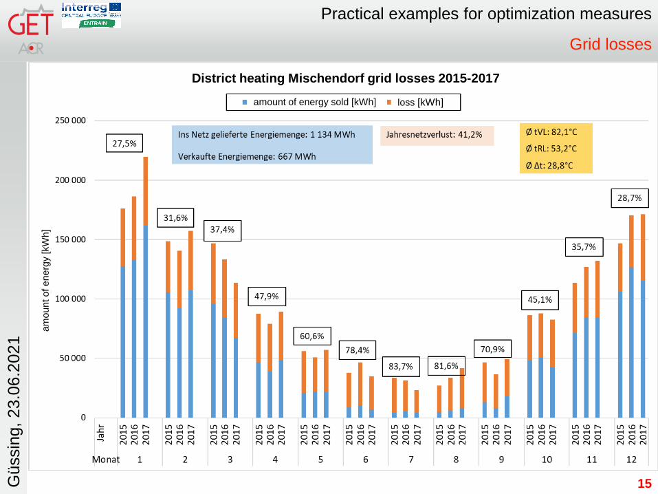
Grid losses
15
District heating Mischendorf grid losses 2015-2017
amount of energy sold [kWh] loss [kWh]
am
ou
nt o
f e
ne
rgy [kW
h]

Practical examples for optimization measuresG
üssin
g, 23.0
6.2
021
Grid pumps – volume flow groups
16
Statistic distribution volume flow groups grid pump FW
Mischendorf 2015 - 2017
volume flow area [m3/h]
sh
are
of
the
to
tal tim
e o
ve
r th
e y
ea
r
Practical examples for optimization measuresG
üssin
g, 23.0
6.2
021
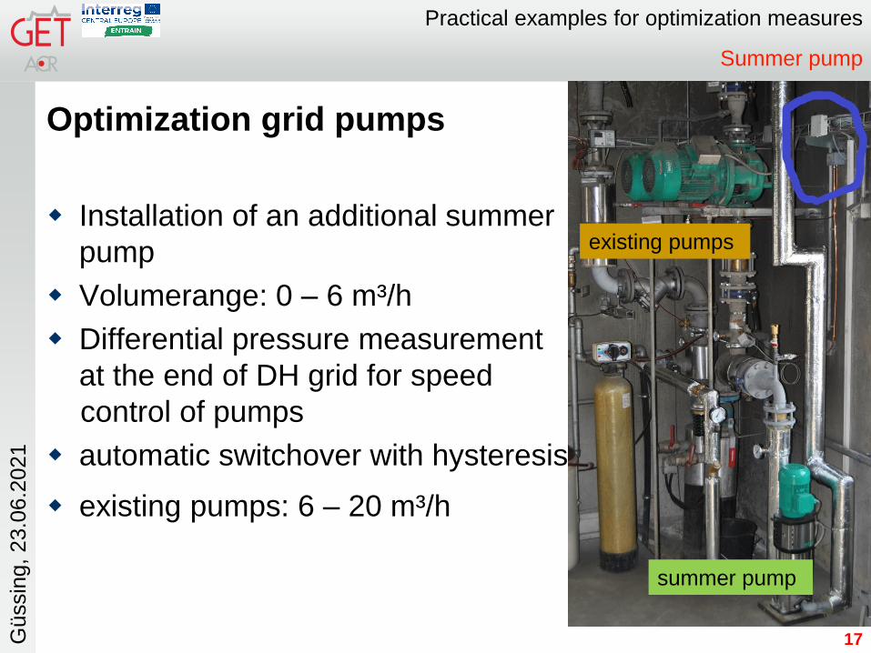
Summer pump
Optimization grid pumps
Installation of an additional summer
pump
Volumerange: 0 – 6 m³/h
Differential pressure measurement
at the end of DH grid for speed
control of pumps
automatic switchover with hysteresis
existing pumps: 6 – 20 m³/h
17
existing pumps
summer pump
Practical examples for optimization measuresG
üssin
g, 23.0
6.2
021
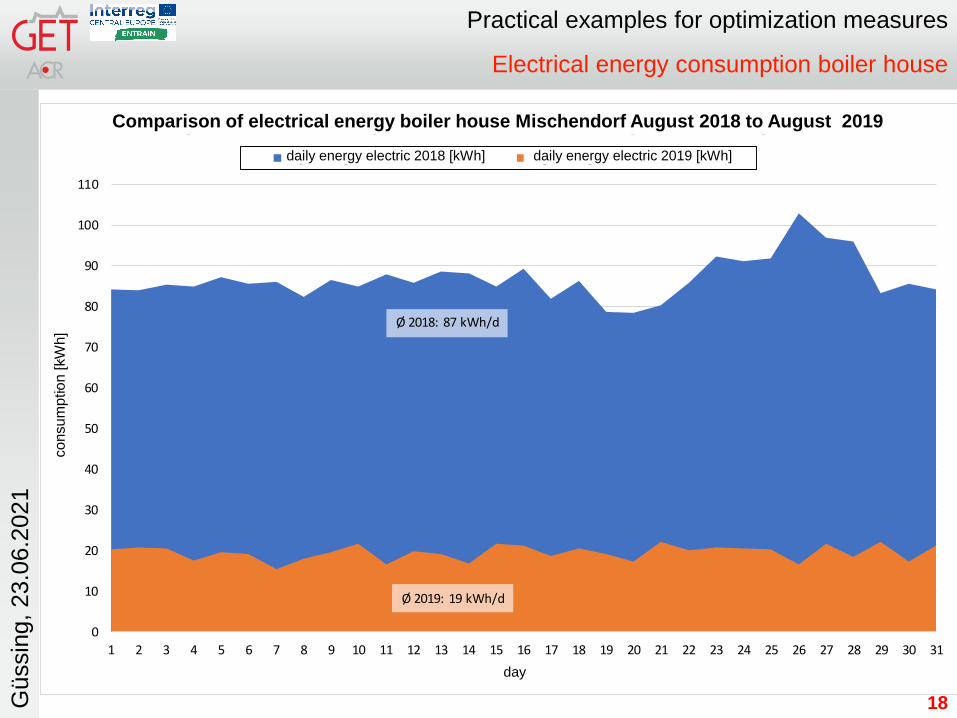
Electrical energy consumption boiler house
18
0
10
20
30
40
50
60
70
80
90
100
110
1 2 3 4 5 6 7 8 9 10 11 12 13 14 15 16 17 18 19 20 21 22 23 24 25 26 27 28 29 30 31
Verb
rauc
h [k
Wh]
Tag
Vergleich elektrische Energie Kesselhaus Mischendorf August 2018 zu August 2019
Tagesenergie elektrisch 2018 [kWh] Tagesenergie elektrisch 2019 [kWh]
Ø 2018: 87 kWh/d
Ø 2019: 19 kWh/d
Comparison of electrical energy boiler house Mischendorf August 2018 to August 2019
daily energy electric 2018 [kWh] daily energy electric 2019 [kWh]
co
nsu
mp
tio
n [kW
h]
day

Practical examples for optimization measuresG
üssin
g, 23.0
6.2
021
Optimization at consumer side
Optimization at customer
side
Analysis of district heating
consumers
Key figures (Ø Dt supply/return)
to classify DH consumers
Optimization usually only makes
economic sense for large
customers
19
Largest consumer (~ 25% heat)
=> problem => on-site analysis

Practical examples for optimization measuresG
üssin
g, 23.0
6.2
021
Optimization at consumer side
On-site analysis customer 1
20
Actual status at the time of inspection
Problem: Pump with const. volume flow between DH heat
exchanger and hydraulic switch
Return temperature to DH heat exchanger rises => mixing
in hydraulic switch
heat exchanger of
the district heating
transfer station
7 branches with
3 way mixing
system
constant
volume flow
Hyd.-switch

Practical examples for optimization measuresG
üssin
g, 23.0
6.2
021
Optimization at consumer side
Troubleshooting customer 1
21
Intelligent pump with DT control and 2
external temperature sensors
Pump minimizes volume flow and
return temperature between the heat
exchanger and hydraulic switch
heat exchanger of
the district heating
transfer station Hyd.-switch
7 x outlets with
mixing circuit

Practical examples for optimization measuresG
üssin
g, 23.0
6.2
021
Optimization at consumer side
22
Volume flow 16 Volume flow 19
Volume: Energy
: Energy
:Volume:
Te
mp
era
ture
[°C
]
Vo
lum
e flo
w[m
3/h
]
Comparison of consumer 1 - 2016 and 2019 - April 6th to may 25th

Practical examples for optimization measuresG
üssin
g, 23.0
6.2
021
Overall Result
23
35
40
45
50
55
60
65
70
75
80
85
0
1
2
3
4
5
6
7
8
9
10
01.04. 01.05. 31.05. 01.07. 31.07. 31.08. 30.09. 30.10.
Tem
pe
ratu
r [°
C]
Vo
lum
en
stro
m [
m³/
h]
FW Mischendorf Netzzähler - Vergleich April - Oktober 2016 / 2019 mit Tagesmittelwerten
Durchfluss 16 [m³/h] Durchfluss 19 [m³/h] VL Temp. 16 [°C] RL Temp. 16 [°C] VL Temp. 19 [°C] RL Temp. 19 [°C]
Mittelwerte April - Oktober 2016Vorlauftemp.: 80,1 °C
Rücklauftemp.: 51,7 °CLeistung: 71,0 kWVolumenstrom: 2,2 m³/hVolumen gep.: 11.263 m³Energiemenge: 364,5 MWhSpreizung: 28,4 °Cspez. Vol.: 30,9 m³/MWh
Mittelwerte April - Oktober 2019Vorlauftemp.: 77,1 °C
Rücklauftemp.: 43,7 °CLeistung: 66,2 kWVolumenstrom: 1,7 m³/hVolumen gep.: 8.481 m³Energiemenge: 340,3 MWhSpreizung: 33,4 °Cspez. Vol.: 24,9 m³/MWh
DH Mischendorf grid heat meter - Comparison April - October 2016/2019 with daily mean values
Flow 16 [m3/h] Flow 19 [m3/h]
Vo
lum
e flo
w [m
3/h
]
Te
mp
era
ture
[°C
]

Practical examples for optimization measuresG
üssin
g, 23.0
6.2
021
Overall Results DH Mischendorf
Result of the optimization measures
Savings of
24

Practical examples for optimization measuresG
üssin
g, 23.0
6.2
021
Basic data DH St. Michael
Basic data for district heating St. Michael
Urbas boiler: 1.700 kW nominal output
Biogas CHP: 280 kW nominal output
Storage 2 x 30 m³
DH network grid: 8.666 trm trench length
115 heat consumers
Annual energy sold to consumers: 3.278 MWh/a
25

Practical examples for optimization measuresG
üssin
g, 23.0
6.2
021
DH network grid
26
Boiler house

Practical examples for optimization measuresG
üssin
g, 23.0
6.2
021
Annual heat capacity duration curve
27
0
200
400
600
800
1.000
1.200
1.400
1.600
1.800
2.000
0 15 30 45 60 75 90 105 120 135 150 165 180 195 210 225 240 255 270 285 300 315 330 345 360
Leis
tun
g [k
W]
Tage
Jahresdauerlinie Leistung Fernwärme St. Michael11/17 bis 11/18to
Annual heat capacity duration curve DH St. Michael
Po
we
r [k
W]
Days

Practical examples for optimization measuresG
üssin
g, 23.0
6.2
021
Network losses measurement data
28
0
100
200
300
400
500
600
700
800
900
1.000
Juli August September Oktober November Dezember Jänner Februar März April Mai Juni
Ener
gie
[MW
h]
Fernwärme St. Michael - Gesamtenergieanalyse 01.07.2016 bis 30.06.2017
verkaufte Energie [MWh] Netzverluste [MWh]
72,2%65,6% 76,4%
33,1%
26,9%
20,3%
18,8%
24,5%
35,6%
39,9%
51,9%
79,3%
Ins Netz gelieferte Energiemenge: 4.816 MWh/averkaufte Energiemenge: 3.259 MWh/aNetzverluste: 1.557 MWh/a
Jahresnetzverluste: 32,3%
Ø tVL: 86 °CØ tRL: 57 °C
Ø Dt: 29 °C
DH St. Michael total energy analysis 01.07.2016 to 30.06.2017
Sold energy [mwh] Network loses [mwh]

Practical examples for optimization measuresG
üssin
g, 23.0
6.2
021
Optimization DH St. Michael
Boiler house optimization steps
Implementation of the network grid pump control by a
pressure loss curve => wire to most unfavourable section
of the grid is damaged
Optimization of the supply temperature over summer
Installation of a summer grid pump
29
Practical examples for optimization measuresG
üssin
g, 23.0
6.2
021
100
150
200
250
300
350
400
450
500
550
600
0
10
20
30
40
50
60
70
80
90
100
01.06. 06.06. 11.06. 16.06. 21.06. 26.06.
Leis
tun
g [k
W]
Vo
rlau
fte
mp
erat
ur
[°C
], R
ück
lau
fte
mp
erat
ur
[°C
], V
olu
men
stro
m [m
³/h
]
FW St. Michael - Vergleich Juni 19 mit Juni 20
Vorlauf 19 Rücklauf 19 Volumenstrom 19 Vorlauf 20
Volumenstrom 20 Rücklauf 20 Leistung 19 Leistung 20
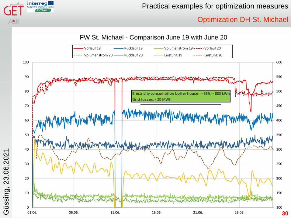
Stromverbrauch Heizhaus: - 55%; - 803 kWhNetzverluste: - 20 MWh
Optimization DH St. Michael
30
FW St. Michael - Comparison June 19 with June 20

Practical examples for optimization measuresG
üssin
g, 23.0
6.2
021
Optimization DH St. Michael
31
Reduction of the network flow temperature to 75 ° C instead of 85 ° C
Return temperature at approx. 46 ° C instead of 55 ° C
Drive power mains pump approx. 150 W instead of approx. 500 W
previously (summer pump)
Practical examples for optimization measuresG
üssin
g, 23.0
6.2
021
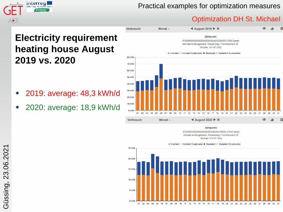
Optimization DH St. Michael
Electricity requirement
heating house August
2019 vs. 2020
2019: average: 48,3 kWh/d
2020: average: 18,9 kWh/d
32

Practical examples for optimization measuresG
üssin
g, 23.0
6.2
021
Pipe network losses calculation
33
Measurement data ~
calculation
no big insulation
damage
Pipe dimension
Grid losses - metering
value: 1.557 MWh/a

Practical examples for optimization measuresG
üssin
g, 23.0
6.2
021
Optimization at consumer side
Minimize network grid losses
Optimization of consumer side
34
Knd.Nr. Name Volumen Ø DT Verbrauch
[m³] [°C] [kWh]
D000250 MARKTGEMEINDE ST.MICHAEL 7.882,7 37,9 339.677
D000240 AUTOHAUS STRAUSS 6.513,0 26,6 197.360
D000339 Unimarkt Handels GmbH & CoKG 5.723,6 13,5 88.120
D000101 MATISOVITS Ges.m.b.H. 5.304,5 24,8 149.371
D000243 GERGER Ges.m.b.H. 4.294,4 16,5 80.400
D000300 EG Meierhofgasse 300 St.Michael 4.144,1 22,3 104.967
D000008 Verein zur Erhaltung und Erneuerung 3.118,2 29,2 103.631
D000010 Boisits-Hadrawa Elisabeth 2.703,2 19,0 58.560
D000015 Kulovits - Freislinger Gisela 2.252,1 34,2 87.521
D000399 OSG Wohnung Hauptzähler 1.703,9 18,3 35.423
D000163 MARKTGEMEINDE ST.MICHAEL 1.623,7 28,5 52.674
D000377 B-SÜD Gemeinn. WohnungsgesmbH 1.563,2 19,4 34.533
Name Volume Consumption

Practical examples for optimization measuresG
üssin
g, 23.0
6.2
021
PV-Investment
PV- Investment
Yield and consumption
profile of boiler house
Target: Maximize
consumption in boiler house
35
Typ. Yield profile PV
FW consumption profile
Total consumption

Practical examples for optimization measuresG
üssin
g, 23.0
6.2
021
PV-Investment
36
0
5
10
15
20
25
30
35
40
45
50
55
60
65
70
75
80
85
90
95
100
0 1 2 3 4 5 6 7 8 9 10 11 12 13 14 15 16 17 18 19 20 21 22 23 24 25
Eige
nve
rbra
uch
squ
ote
[%
]
Leistung [kWp]
Eigenverbrauchsquote HW St. Michael
Se
lf-c
on
su
mp
tio
nra
te [%
]
Self-Consumption rate DH St. Michael
Power [kWp]
Calculations based on hourly values
Annual consumption: 51,7 MWhel

Practical examples for optimization measuresG
üssin
g, 23.0
6.2
021
Conclusion and learnings
Conclusion and learnings on practical
examples
Metering data is the most important source of
information
DH network grid pumps => often potential to save
electricity
Minimize return temperature level
Optimization at consumer side
◼ Start with big consumers
◼ Check average Dt [°C] or specific pump energy [m³/MWh]
37

Practical examples for optimization measuresG
üssin
g, 23.0
6.2
021
Conclusion
Contact
Dipl. Ing. (FH) Klaus Paar
Güssing Energy Technologies GmbH
Forschungsinstitut für erneuerbare Energie
Wiener Straße 49
A-7540 Güssing
Tel./Phone: +43 3322 42606 322
Mobil: +43 676 430 81 91
mail: [email protected]
URL: http://get.ac.at
38