Power, Precision, and Sample Size Calculations Notes/PowerInSem...Power, Precision, and Sample Size Calculations 1 Introduction 2 Hypothesis Testing and Fit Evaluation: What, Where,

Power, Precision, and Sample Size Calculations

James H. Steiger

Department of Psychology and Human DevelopmentVanderbilt University

James H. Steiger (Vanderbilt University) Power, Precision, and Sample Size Calculations 1 / 49

Power, Precision, and Sample Size Calculations1 Introduction

2 Hypothesis Testing and Fit Evaluation: What, Where, How, and Why

Testing the Model for Perfect Fit

Testing for Close Fit

Testing for Not-Close Fit

Testing Individual Parameters

3 Power Charts for Tests of Overall Model Fit

4 Sample Size Calculations for Tests of Model Fit

Sample Size Tables

5 Interval Estimation Approaches

Changing the Emphasis – AIPEJames H. Steiger (Vanderbilt University) Power, Precision, and Sample Size Calculations 2 / 49

Introduction

Introduction

One of the key decisions prior to initiating a research study using SEM is the choice of asample size for the study.We’ve already seen how the wrong choice can lead to a high probability of failure in thecase of confirmatory factor analysis, because of a lack of convergence.Besides issues of convergence, we also have the problems of power and precision, whicharise in all areas of statistics.In this module, we’ll review several approaches to power, precision, and sample sizeestimation in SEM, and conclude with some computational examples.We’ll stick to the multivariate normal model with single samples, but many of the pointsand techniques discussed here will generalize to other situations.We’ll begin with classical hypothesis testing considerations, then move on the the moremodern confidence interval perspective.


Hypothesis Testing and Fit Evaluation: What, Where, How, and Why

Hypothesis Testing and Fit Evaluation: What, Where, How, and Why

Let’s begin by recalling some of the standard types of hypotheses that are tested in SEM.1 Evaluating whether a model fits perfectly.2 Evaluating whether it fits “signicantly worse than good.”3 Evaluating whether it fits “significantly better than bad.”4 Testing whether one model fits better than another model it is nested within.5 Evaluating the badness of fit of a model with a point estimate and a confidence interval.6 Estimating model parameters and establishing a confidence interval.


Hypothesis Testing and Fit Evaluation: What, Where, How, and Why Testing the Model for Perfect Fit

Hypothesis Testing and Fit Evaluation: What, Where, How, and WhyTesting the Model for Perfect Fit

The standard χ2 statistic tests for perfect model fit.If fit is perfect, this statistic has an asymptotic chi-square distribution with p(p + 1)/2 − tdegrees of freedom, where p is the number of variables and t the number of (truly) freeparameters in the model.This statistic is calculated in maximum likelihood estimation as

X = kFML (1)

where FML is the standard Maximum Wishart Likelihood discrepancy function, and k is ascaling constant usually equal to n − 1.Other scaling constants — in particular one proposed by Swain in the context ofcovariance structure modeling and another by Bartlett in the context of factor analysis,may be used to attempt to improve performance at small sample sizes.Of course, if fit is not perfect in the population, then the test statistic will no longer havea χ2 distribution.




Strictly speaking, if the population covariance structure model does not fit the populationΣ perfectly, then the distribution of the test statistic diverges.We might choose to measure how badly a model fits in the population by fitting themodel to the population Σ with the method of maximum likelihood and using the“population discrepancy function” F ∗ as our measure of misfit.Steiger, Shapiro, and Browne (1985) invoked a special assumption called “populationdrift,” which imagines that the population parameters, rather than being stable, aredrifting along with sample size toward a point at which model fit is perfect.This assumption models the situation in which fit is not too bad relative to sample size.This assumption leads to a distributional result, i.e., that the asymptotic distribution ofthe χ2 statistic is noncentral χ2, with noncentrality parameter given by

(n − 1)F ∗ML (2)

in the standard case in which k = n − 1 is used as the multiplier.




The noncentral χ2 approximation can furnish accurate estimates of the performance ofthe likelihood ratio test statistic when the null hypothesis is false.One employs the standard approach of first obtaining a rejection point from the centralchi-square distribution, then computing the probability in the rejection region under thealternative hypothesis.




Suppose you have a structural equation model based on p = 7 variables with t = 6 freeparameters. The population discrepancy function is 0.055. What is the power of the testof perfect fit if α = 0.05, 1-sided and n = 185?Using R, we first establish the critical value (rejection point).

> p <- 7

> t <- 6

> F.ML <- 0.055

> df <- p*(p+1)/2

> df

[1] 28

> critical.value <- qchisq(0.95,df)

> critical.value

[1] 41.33714




Now we compute the power.First we calculate the noncentrality parameter.

> n <- 185

> lambda = (n-1)*F.ML

> lambda

[1] 10.12

Next we compute the power.

> power <- 1 - pchisq(critical.value,df,lambda)

> power

[1] 0.3443796

We find that the power is 0.344.




Note how straightforward power calculation is. However, a key point was glossed over:How does one estimate the population discrepancy function?MacCallum, Browne, and Sugawara (1996) suggested using the RMSEA as a vehicle forestimating an alternative value of the discrepancy function. Recall that, in thepopulation, the RMSEA is defined as

ε =

√F ∗ML

df(3)

Consequently,F ∗ML = ε2 × df (4)

If one can specify a “non-trivial” RMSEA cut-off, one can use that to compute adiscrepancy function, and from that discrepancy function compute the noncentralityparameter, followed by power.




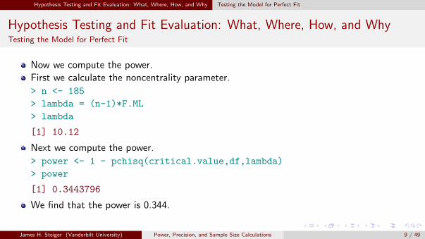
Suppose, for example, the minimal RMSEA is 0.08. You want to have a guaranteed levelof power to detect an RMSEA that small.In the present example, this RMSEA would translate into a noncentrality parameter asfollows.

> epsilon <- 0.08

> F.ML <- epsilon^2 * df

> F.ML

[1] 0.1792

> lambda <- (n-1)*F.ML

> power <- 1 - pchisq(critical.value,df,lambda)

> power

[1] 0.9366569

We find that power to reject the hypothesis of perfect fit is 0.937 if the RMSEA is 0.08 inthe population.


Hypothesis Testing and Fit Evaluation: What, Where, How, and Why Testing for Close Fit

Hypothesis Testing and Fit Evaluation: What, Where, How, and WhyTesting for Close Fit

In some cases, one may not wish to test that fit is perfect.For example, MacCallum, Browne, and Sugawara(1996) discussed two other kinds of tests,which they referred to as the test of close fit and the test of not-close fit, respectively.




The standard χ2 test of perfect fit is also a test of the hypothesis that the RMSEA isequal to zero in the population.The test of close fit assumes as its statistical null hypothesis not that the populationRMSEA is zero, but rather that it is less than or equal to some other reasonable value.For example, suppose the null hypothesis is

H0 : ε ≤ 0.05 (5)

The alternative isH0 : ε > 0.05 (6)




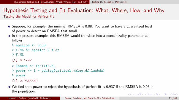
This is a 1-sided test.The rejection region begins at a critical value at the 1 − α quantile of the noncentral χ2

distribution.Here is a sample problem. Suppose the test of close fit is performed as before withn = 185, p = 7, and t = 6, and α = 0.05.What is the power to reject H0 if the true population RMSEA is 0.08?




First we calculate the null distribution and rejection point.Although the null hypothesis specifies a region rather than a point, we can make ourpoint of calculation the boundary of that region, at ε = 0.05. Then power will be at leastas large as the calculated value.

> epsilon0 <- 0.05; epsilon1 <- 0.08; df <- p * (p+1) /2 - t

> alpha <- 0.05; n<-185

> F0 <- epsilon0^2 *df

> lambda0 <- (n-1) * F0

> critical.value <- qchisq(1-alpha, df, lambda0)

> F1 <- epsilon1^2 * df

> lambda1 <- (n-1) * F1

> power <- 1 - pchisq(critical.value,df,lambda1)

> power

[1] 0.4504781


Hypothesis Testing and Fit Evaluation: What, Where, How, and Why Testing for Not-Close Fit

Hypothesis Testing and Fit Evaluation: What, Where, How, and WhyTesting for Not-Close Fit

The original χ2 test of perfect fit suffered from several problems:1 It was unrealistic. The assumption of perfect fit is extremely unlikely to be correct.2 It is an Accept-Support test. Supporting a proposed model requires not rejecting the null

hypothesis. Accept-Support testing suffers from a number of problems. In particular, itrewards low power and sloppy experimentation.




The test of close fit improves on the test of perfect fit, in that it tests a more reasonablenull hypothesis.However, it is still an Accept-Support procedure, in that it requires not rejecting the nullhypothesis to support a model.




The test of not-close fit takes a different approach.The null hypothesis is now stated in the form

H0 : ε ≥ ε0 (7)

where ε0 is a value that represents “reasonably good fit.”Since the alternative hypothesis is

H1 : ε < ε0 (8)

rejection of the null implies that “fit is significantly better than reasonably good.”




The test of not-close fit eliminates the problems associated with Accept-Support testing.This test is easy to perform, and to calculate power for.Suppose we wish to test the null hypothesis that ε ≥ 0.05, and the true state of the worldis that ε = 0.01.In that case, the power will be as calculated below. Note that now the rejection region ison the low side of the null hypothesized distribution.

> epsilon0 <- 0.05; epsilon1 <- 0.01

> F0 <- df * epsilon0^2

> lambda0 <- (n-1)*F0

> critical.value <- qchisq(0.05,df,lambda0)

> F1 <- df * epsilon1^2

> lambda1 <- (n-1)*F1

> power <- pchisq(critical.value,df,lambda1)

> power

[1] 0.3062439


Hypothesis Testing and Fit Evaluation: What, Where, How, and Why Testing Individual Parameters

Hypothesis Testing and Fit Evaluation: What, Where, How, and WhyTesting Individual Parameters

So far, we have been discussing tests on an entire model.Such tests can be useful, and power analysis for such tests is straightforward.Another kind of test performed frequently in the context of structural equation modelingis the test of significance on a parameter.Two types of tests can be performed:

1 The χ2 difference test.2 The Wald test.

In the χ2 difference test, two models are tested, with and without the path involving theparameter of interest.In the Wald test, the model is fit with the parameter of interest included, and anasymptotically normal test statistic is computed by dividing the parameter by its(estimated) standard error.




A model without a path containing a parameter is nested within a model containing theparameter.Consequently, a result of Steiger, Shapiro, and Browne (1985) can be applied.Under fairly general conditions, the difference between the chi-square tests for two nestedmodels is distributed as noncentral χ2 with degrees of freedom equal to the difference indegrees of freedom for the two models (i.e., in this case 1), and a noncentrality parameterequal to the difference in noncentrality parameters for the two models.Consequently, one may estimate power to reject the null hypothesis for a single parameterby a two step process:

1 Create the population covariance matrix corresponding to the model with the pathcontaining the parameter.

2 Fit this matrix to the model without the path containing the parameter, thereby obtaining anon-zero population discrepancy function, and through it, a noncentrality parameter.

3 Use the non-central χ2 approximation to compute the power.




Here is an example. Suppose that the following factor pattern fit the populationcovariance matrix perfectly. Note there is one unanticipated “crossover loading” markedin red.

Λ =

0.7 0.0 0.00.7 0.0 0.00.7 0.0 0.00.0 0.7 0.00.0 0.7 0.00.0 0.7 0.00.0 0.2 0.70.0 0.0 0.70.0 0.0 0.7

(9)




We generate the covariance matrix corresponding to Λ. First we construct Λ in R.

> Lambda <- matrix(c(rep(.7,3),rep(0,9),rep(0.7,3),

+ 0.2,rep(0,8),rep(.7,3)),9,3)

> Lambda

[,1] [,2] [,3]

[1,] 0.7 0.0 0.0

[2,] 0.7 0.0 0.0

[3,] 0.7 0.0 0.0

[4,] 0.0 0.7 0.0

[5,] 0.0 0.7 0.0

[6,] 0.0 0.7 0.0

[7,] 0.0 0.2 0.7

[8,] 0.0 0.0 0.7

[9,] 0.0 0.0 0.7




Next, we apply one of the utility functions.

> MakeFactorCorrelationMatrix <- function(F){

+ r <-F %*% t(F)

+ h <- diag(r)

+ u <- diag(1 - h)

+ r <- r+u

+ r

+ }

> R <- MakeFactorCorrelationMatrix(Lambda)

> R

[,1] [,2] [,3] [,4] [,5] [,6] [,7] [,8] [,9]

[1,] 1.00 0.49 0.49 0.00 0.00 0.00 0.00 0.00 0.00

[2,] 0.49 1.00 0.49 0.00 0.00 0.00 0.00 0.00 0.00

[3,] 0.49 0.49 1.00 0.00 0.00 0.00 0.00 0.00 0.00

[4,] 0.00 0.00 0.00 1.00 0.49 0.49 0.14 0.00 0.00

[5,] 0.00 0.00 0.00 0.49 1.00 0.49 0.14 0.00 0.00

[6,] 0.00 0.00 0.00 0.49 0.49 1.00 0.14 0.00 0.00

[7,] 0.00 0.00 0.00 0.14 0.14 0.14 1.00 0.49 0.49

[8,] 0.00 0.00 0.00 0.00 0.00 0.00 0.49 1.00 0.49

[9,] 0.00 0.00 0.00 0.00 0.00 0.00 0.49 0.49 1.00




We can save the correlation matrix to a text file for analysis by Mplus.

> Rout <- data.frame(R)

> write.table(Rout,"PowerCov.dat",row.names=FALSE,

+ col.names=FALSE,sep=" ")




Next we analyze the data with Mplus, leaving out the path corresponding to the crossoverloading.

TITLE: SETUP ANALYSIS FOR POWER CALCULATION;

DATA: FILE IS PowerCov.dat;

TYPE IS FULLCOV;

NOBSERVATIONS = 1000000;

VARIABLE: NAMES ARE Y1-Y9;

MODEL: F1 BY Y1-Y3*;

F2 BY Y4-Y6*;

F3 BY Y7-Y9*;

F1-F3@1;




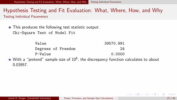
This produces the following test statistic output:

Chi-Square Test of Model Fit

Value 39570.991

Degrees of Freedom 24

P-Value 0.0000

With a “pretend” sample size of 106, the discrepancy function calculates to about0.03957.




Suppose sample size was actually 250 with this population matrix.Then the population noncentrality parameter would be

> F <- 0.03957

> Lambda = (250-1) * F

> Lambda

[1] 9.85293

> epsilon = sqrt(F/24)

> epsilon

[1] 0.0406048

The difference test has one degree of freedom, and we estimate the power as

> critical.value <- qchisq(0.95,1)

> power <- 1 - pchisq(critical.value, 1, Lambda)

> power

[1] 0.8807959

Power is about 0.88.




On the other hand, the test of perfect model fit has 24 degrees of freedom, so the powerto reject perfect model fit is lower.

> critical.value <- qchisq(0.95,24)

> power <- 1 - pchisq(critical.value, 24, Lambda)

> power

[1] 0.3614827

Power for this test is estimated to be only 0.361


Power Charts for Tests of Overall Model Fit


Constructing a power chart, displaying power as a function of sample size or some otherquantity, is really straightforward in R.Let’s begin by constructing a power function, that returns estimated power as a functionof α, ε0, ε1, df , and n.




> ## Calculate power as a function of

> ## n Sample Size

> ## epsilon1 The true population RMSEA

> ## epsilon0 The null RMSEA (0 for a test of perfect fit)

> ## alpha Type I Error Rate

> ## tail "lower" or "upper" (Where the rejection region is)

> SEMpower <- function(n,df,epsilon1,epsilon0=0,alpha=0.05,tail="upper"){

+ lambda0 <- (n-1)*df*epsilon0^2

+ lambda1 <- (n-1)*df*epsilon1^2

+ critical.p <- if(tail == "upper") 1-alpha else alpha

+ critical.value <- qchisq(critical.p,df,lambda0)

+ critical.prob <- pchisq(critical.value,df,lambda1)

+ power <- if (tail == "upper") 1-critical.prob else critical.prob

+ return(power)

+ }




Let’s try out our function on the example we just worked.In that example, we had a population discrepancy function of F = 0.03957, which,combined with 24 degrees of freedom, translates into a population RMSEA of

ε =

√0.03957

24= 0.0406048 (10)

For a test of perfect fit, ε0 = 0.We can calculate power (using the default upper tail and α = 0.05) as

> SEMpower(250,24,sqrt(0.03957/24))

[1] 0.3614827




We can now display a power chart showing power as a function of n for this situation.

> curve(SEMpower(x,24,0.0406),100,1000,col="red",

+ xlab="Sample Size (n)",

+ ylab="Power")

200 400 600 800 1000

0.2

0.4

0.6

0.8

1.0

Sample Size (n)

Pow

er




The SEMpower function can be adapted to handle situations in which a test of close-fit,or a test of not-close fit is being performed.It can also be used to estimate the sample size required to achieve a guaranteed level ofpower under specified conditions, as shown in the next section.


Sample Size Calculations for Tests of Model Fit


In the just-completed analysis, we found of power of 0.36, certainly not adequate.The question immediately arises: What would sample size n have to be to yield anacceptable level of power?In this situation, there is no direct analytic solution to the required sample size. Thesolution can be approximated reasonably well, or calculated precisely by iterative methods.The method of bisection works quite well in this case, and is extraordinarily simple.The calculation is hampered slightly by the fact that, in the final analysis, n must be aninteger.




A function calculating required sample size is a good one to have, and we’ll develop oneeventually.However, for one specific situation, one doesn’t need to go to this trouble.Instead, we use a simple graphical approach.Remember this approach well, as you may find it useful in the future. It is, in general,much easier to construct a power calculation function than it is to construct a sample sizecalculating function!




What sample size would be required to guarantee a power of 0.90? Looking at thepreviously generated graph, we can begin by adding a horizontal line at 0.90.Simple inspection tells us that the required n is between 650 and 750.



+ ylab="Power")

> abline(h = 0.90, col="blue")

200 400 600 800 1000

0.2

0.4

0.6

0.8

1.0

Sample Size (n)

Pow

er




We redraw the graph with narrower limits of 650 and 750.We add gridlines in grey to help us.We can see that the required n is clearly between 705 and 710, and is almost certainlyeither 707 or 708.



+ ylab="Power")


> abline(v = seq(650,750,10), col="grey")

660 680 700 720 740

0.87

0.88

0.89

0.90

0.91

0.92

Sample Size (n)

Pow

er




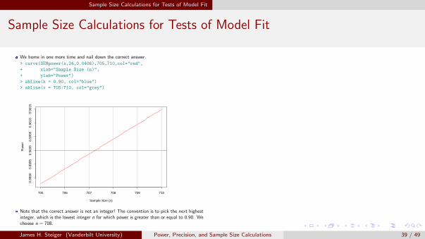
We home in one more time and nail down the correct answer.



+ ylab="Power")


> abline(v = 705:710, col="grey")

705 706 707 708 709 710

0.89

900.

8995

0.90

000.

9005

0.90

100.

9015

Sample Size (n)

Pow

er

Note that the correct answer is not an integer! The convention is to pick the next highestinteger, which is the lowest integer n for which power is greater than or equal to 0.90. Wechoose n = 708.


Sample Size Calculations for Tests of Model Fit Sample Size Tables

Sample Size Calculations for Tests of Model FitSample Size Tables

Using an iterative algorithm, it is easy to construct tables or charts of sample sizesrequired to achieve a given level of power.Here are some examples from MacCallum, Browne, and Sugawara (1996).What are some “take home” messages from the tables? (C.P.)



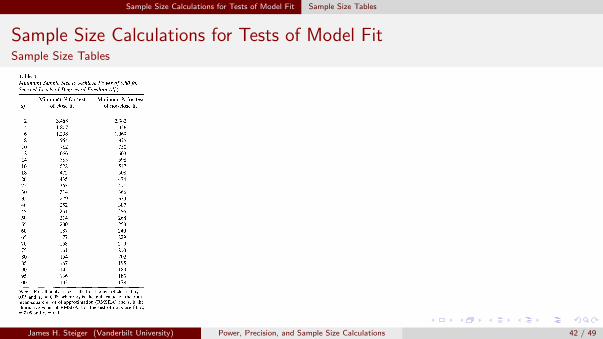
Sample Size Calculations for Tests of Model FitSample Size Tables POWER ANALYSIS IN CSM 145

Table 5Minimum Sample Sizes for Test of Exact Fit forSelected Levels of Degrees of Freedom (df) andPower

df

2468101214161820253035404550556065707580859095100

Minimum Nfor power = 0.80

1,9261,194910754651579525483449421368329300277258243230218209200193186179174168164

Minimum Nfor power = 0.50

994644502422369332304280262247218196180167157148140134128123119115111108105102

Note. The a = .05, e,, = 0.0, and ea = 0.05, where e,, is thenull value of the root-mean-square error of approximation(RMSEA) and e, is the alternative value of RMSEA.

An additional phenomenon of interest shownby the results in Table 4 is that the Nmm values forthe two cases cross over as d increases. At lowvalues of d, Nmm for the test of close fit is largerthan Nmin for the test of not-close fit. For d > 14,the relationship is reversed. This phenomenon isattributable to the interactive effect of effect sizeand d on power. The effect size represented bythe test of close fit (e0 = 0.05 and ea = 0.08) is aneffectively larger effect size than that for the testof not-close fit (EO = 0.05 and sa = 0.01) at higherlevels of d but is effectively smaller at lower levelsold.

Let us finally consider determination of Nmm fora third case of interest, the test of exact fit when

ea = 0.05. Using a = .05, Table 5 shows values ofyVmin for selected levels of d, for two levels of de-sired power, 0.80 and 0.50. These results provideexplicit information about the commonly recog-nized problem with the test of exact fit. Levels ofNmm for power of 0.80 reflect sample sizes thatwould result in a high likelihood of rejecting thehypothesis of exact fit when true fit is close. Corre-sponding levels of yVmin for power of 0.50 reflectsample sizes that would result in a better than 50%chance of the same outcome. For instance, withd = 50 and N > 243, the likelihood of rejectingthe hypothesis of exact fit would be at least .80,even though the true fit is close. Under the sameconditions, power would be greater than 0.50 withN > 148. As d increases, the levels of N that pro-duce such outcomes become much smaller. Theseresults provide a clear basis for recommendingagainst the use of the test of exact fit for evaluatingcovariance structure models. Our results showclearly that use of this test would routinely resultin rejection of close-fitting models in studies withmoderate to large sample sizes. Furthermore, it ispossible to specify and test hypotheses aboutmodel fit that are much more empirically relevantand realistic, as has been described earlier inthis article.

For the five empirical studies discussed earlierin this article, Table 3 shows values of /Vmin forachieving power of 0.80 for the tests of close fitand not-close fit. These results are consistent withthe phenomena discussed earlier in this section.Most important is the fact that rigorous evaluationof fit for models with low d, such as those studiedby Meyer and Gellatly (1988) and Vance and Col-ella (1990), requires extremely large N. Such mod-els are not rare in the literature. Our results indi-cate that model evaluation in such cases is highlyproblematic and probably should not be under-taken unless very large samples are available.

Comparison to Other Methods forPower Analysis in CSM

As mentioned earlier, there exists previous liter-ature on power analysis in CSM. Satorra and Saris(1983, 1985; Saris & Satorra, 1993) have proposeda number of techniques for evaluating power of thetest of exact fit for a specific model. The methodspresented in this earlier work are based on thesame assumptions and distributional approxima-



Sample Size Calculations for Tests of Model FitSample Size Tables144 MAcCALLUM, BROWNE, AND SUGAWARA

Table 4Minimum Sample Size to Achieve Power of 0.80 forSelected Levels of Degrees of Freedom (df)

dfMinimum N for test

of close fitMinimum N for test

of not-close fit

2468101214161820253035404550556065707580859095100

3,4881,8071,238954782666585522472435363314279252231214200187177168161154147142136132

2,3821,4261,069875750663598547508474411366333307286268253240229219210202195189183178

Note. For all analyses, a = .05. For the test of close fit. e,, =0.05 and ea = 0.08, where e0 is the null value of the root-mean-square error of approximation (RMSEA) and ea is thealternative value of RMSEA. For the test of not-close fit, e (>= 0.05 and ea = 0.01.

in d causes substantial reduction in power ofmodel tests.

Let us next focus on levels of necessary N as dbecomes larger. As is indicated in Table 4, ade-quate power for the recommended tests can beachieved with relatively moderate levels of N whend is not small. For instance, with d = 100, a powerof 0.80 for the test of close fit (in comparison withthe alternative that ea = 0.08) is achieved withN = 132. Again, such results reflect the behaviorof CIs for e. With large d, relatively narrow CIs areobtained with only moderate N. This phenomenonhas important implications for tests of model fitusing hypotheses about e. For instance, using the

test of close fit, if d is large and actual fit is medio-cre or worse, one does not need a very large sampleto have a high probability of rejecting the falsenull hypothesis. Consider a specific example toillustrate this point. Suppose one has p = 30 mani-fest variables, in which case there would bep(p + l)/2 = 465 distinct elements in thep X p covariance matrix. If we tested the nullmodel that the measured variables are uncorre-lated, the model would have q = 30 parameters(variances of the manifest variables), resulting ind = p(p + 1)12 ~ q = 435. For the test of closefit, in comparison with the alternative that ea =0.08, we would find Nmm = 53 for power of 0.80.That is, we would not need a large sample to rejectthe hypothesis that a model specifying uncorre-lated measured variables holds closely in the popu-lation. In general, our results indicate that if d ishigh, adequately powerful tests of fit can be carriedout on models with moderate N.

This finding must be applied cautiously in prac-tice. Some applications of CSM may involve mod-els with extremely large d. For instance, factoranalytic studies of test items can result in modelswith d > 2000 when the number of items is as highas 70 or more. For a model with d = 2000, a powerof 0.80 for the test of close fit (in comparison withthe alternative that ea = 0.08) can be achievedwith Nmm = 23 according to the procedures wehave described. Such a statement is not meaningfulin practice for at least two reasons. First, one musthave N > p to conduct parameter estimation usingthe common ML method. Second, and more im-portant, our framework for power analysis is basedon asymptotic distribution theory, which holdsonly with sufficiently large N. The noncentral x1

distributions on which power and sample size cal-culations are based probably do not hold theirform well as N becomes small, resulting in inaccu-rate estimates of power and minimum N. There-fore, results that indicate a small value of Nmm

should be treated with caution. Finally, it mustalso be recognized that we are considering deter-mination of 7Vmin only for the purpose of modeltesting. The magnitude of N affects other aspectsof CSM results, and an N that is adequate for onepurpose might not be adequate for other purposes.For example, whereas a moderate N might be ade-quate for achieving a specified level of power fora test of overall fit, the same level of N may notnecessarily be adequate for obtaining precise pa-rameter estimates.


Interval Estimation Approaches


An alternative to a hypothesis-testing framework is based on confidence intervalestimation.One can perform all the standard hypothesis tests discussed above simply by constructinga confidence interval on the RMSEA.Since the tests are one-sided, one constructs a 1 − 2α confidence interval and examines itto see if the confidence interval excludes the critical value of the RMSEA.




Constructing a confidence interval on the RMSEA requires an iterative proceudre.The method is discussed in detail in the article by Steiger and Fouladi (1997) available onmy website in the Publications section.Briefly — One solves inversely for those values of λ that would place the observed data atthe 95th and 5th percentile of the non-central chi-square distribution. These values arethe endpoints of a 90% confidence interval for λ, which may be converted into aconfidence interval for the RMSEA ε.




Suppose, for example, one calculates the 90% CI for ε, and it has endpoints 0 and 0.0491.Could one reject the hypothesis of perfect fit? How about the hypothesis of close fit, withH0 ε ≤ 0.05?Could one reject the hypothesis of not-close fit, if H0 is

H0 : ε ≥ 0.05 (11)




Suppose the confidence interval on the RMSEA has endpoints of 0.0471 and 0.0752.Could one reject the hypothesis of perfect fit?Could one reject the hypothesis of close fit?Could one reject the hypothesis of not-close fit?


Interval Estimation Approaches Changing the Emphasis – AIPE

Interval Estimation ApproachesChanging the Emphasis – AIPE

In the preceding section, we examined several types of hypothesis tests that can beperformed simultaneously with a confidence interval.Only one of the hypothesis tests — the test of not-close fit — involves a Reject-Supportstrategy.The original sample size table from MacCallum, Browne, and Sugawara (1996) involves anull hypothesis that ε ≥ 0.05. Power is calculated under the very stringent alternativehypothesis that ε = 0.01.Clearly, to get a rejection using this strategy requires a narrow confidence interval,because the interval has to fit between 0 and 0.05 in order for a rejection to occur!If your confidence interval is wider than 0.05, this can never happen!




As sample size increases, the average width of a confidence interval for ε generallydecreases.The expected value of the width of a confidence interval is a complex function of thesample size and the RMSEA itself.However, one can estimate the sample size required to produce a “narrow-enough”confidence interval for the RMSEA under a reasonable set of assumptions.This approach of calculating sample size in terms of the expected width of a confidenceinterval has been called AIPE (Accuracy in Parameter Estimation) by Ken Kelley of NotreDame, who has a number of interesting articles on the topic.Some of these techniques are implemented in his MBESS package for R. MBESS alsoimplements confidence interval calculation for the RMSEA.




Here is an example (the package is currently broken )

> ##library(MBESS)

> ##ss.aipe.rmsea(0.03,24,0.08,0.9)


Documents

Power, Precision, and Sample Size Calculations Notes/PowerInSem...Power, Precision, and Sample Size Calculations 1 Introduction 2 Hypothesis Testing and Fit Evaluation: What, Where,