Embed Size (px)
Citation preview
Article
Power Management Strategy of Hybrid ElectricVehicles Based on Quadratic Performance IndexChaoying Xia * and Cong Zhang
Received: 27 July 2015 ; Accepted: 22 October 2015 ; Published: 4 November 2015Academic Editor: K.T. Chau
School of Electrical Engineering and Automation, Tianjin University, No. 92 Weijin Road, Tianjin 300072,China; [email protected]* Correspondence: [email protected]; Tel.: +86-22-8789-2977
Abstract: An energy management strategy (EMS) considering both optimality and real-timeperformance has become a challenge for the development of hybrid electric vehicles (HEVs) in recentyears. Previous EMSes based on the optimal control theory minimize the fuel consumption, butcannot be directly implemented in real-time because of the requirement for a prior knowledge ofthe entire driving cycle. This paper presents an innovative design concept and method to obtaina power management strategy for HEVs, which is independent of future driving conditions. Aquadratic performance index is designed to ensure the vehicle drivability, maintain the batteryenergy sustainability and average and smooth the engine power and motor power to indirectlyreduce fuel consumption. To further improve the fuel economy, two rules are adopted to avoidthe inefficient engine operation by switching control modes between the electric and hybrid modesaccording to the required driving power. The derived power of the engine and motor are related tocurrent vehicle velocity and battery residual energy, as well as their desired values. The simulationresults over different driving cycles in Advanced Vehicle Simulator (ADVISOR) show that theproposed strategy can significantly improve the fuel economy, which is very close to the optimalstrategy based on Pontryagin’s minimum principle.
Keywords: hybrid electric vehicle; linear quadratic optimal control; real-time control;energy management
1. Introduction
As increasingly concerning on the deterioration in air quality and decrease in petroleumresources, a great interest is shown in the development of safe, clean, and high-efficienttransportation. It has been well recognized that the electric vehicle (EV), hybrid electric vehicle(HEV), and fuel cell electric vehicle (FCEV) are the most promising solution to the problem of landtransportation in the future [1]. Since showing improvement in fuel consumption with minimumextra cost, HEVs are considered to offer the best promise in the short to mid-term [2]. In HEVs, theinternal combustion engine (ICE) provides driving power together with one or more reversible energystorage systems (ESSes), such as a bank of batteries and ultra-capacitors, which are generally usedas an energy buffering unit to recycle braking energy and change engine operating points as wellas provide an extra degree of freedom for energy management strategies (EMSes). Undeniably, theintroduction of ESSes makes driving modes more flexible but EMSes more complicated. Therefore, itis especially important to design an excellent EMS for HEV development and application [3,4].
As early as 1997, Jalil used a set of predefined rules based on the battery state of charge (SOC)and power demand to assign the power to the engine, battery, or a combination of both, for a seriesHEV to ensure the high efficiency of the engine and battery operation [5]. Such rule-based strategiesdeveloped from heuristic ideas are widely used in HEVs [6–8] because they can be implemented
Energies 2015, 8, 12458–12473; doi:10.3390/en81112325 www.mdpi.com/journal/energies

Energies 2015, 8, 12458–12473
in real-time, but making rules commonly depends on engineering experience, known mathematicalmodels, large numbers of experimental results, etc., having limited benefits for fuel economy.In order to improve the fuel economy of rule-based methods, Schouten and Duan directly adoptedfuzzy rules instead of deterministic ones to improve the operation efficiency of vehicle system in2002 and 2003 [9,10]. Zhao added a fuzzy algorithm to modify the rules in 2013 [11]. However, thefuel-saving potential of HEVs cannot be fully exploited because the membership functions and rulesof a fuzzy controller are designed based on human expertise and heuristics. To further reduce fuelconsumption, fuzzy controllers were modified by offline optimizing membership functions and rulesthrough a particle swarm optimization algorithm [12], a genetic algorithm [13], or a machine learningalgorithm [14]. Alternatively, a learning vector quantization neural network [15] or a fuzzy neuralnetwork [16] is used in a fuzzy EMS to identify the driving cycle style periodically.
By contrast with above heuristic-based strategies, EMSes based on optimal control theory, suchas dynamic programming (DP) and Pontryagin’s minimum principle (PMP) have been investigatedquite intensively in recent years. For a prior known driving cycle, DP discretizes continuous statesand control values into finite grids and decomposes the overall dynamic optimization probleminto a sequence of sub-problems. The cost function of each sub-problem is the fuel consumptionfrom current step to last step. By calculating backwards along the horizon based on Bellman’sPrinciple of Optimality, DP generated an optimal EMS of HEVs, but with a large computationalload that exponentially increases as the state variables increase in number [17–20]. Theoretically, ifthe whole driving cycle is known in advance and the performance index is defined as an integralof fuel consumption rate, the EMS obtained from DP will minimize the total fuel consumption.However, such an optimal solution is only suitable for the known driving cycle rather than otherones. The requirement for future driving demands to be known in advance leads to a real-timeproblem, so DP always acts as a benchmark to assess other EMSs [21,22]. To apply the optimalresults of DP in real-time, many attempts have been made, such as extracting rules from optimalresults [23,24], modeling the power demand as a random Markov chain [25,26] or predicting futuredriving conditions [27–29].
As another popular theory-based method, PMP formulates the optimal control problem of HEVsas a two-point boundary value problem of nonlinear differential equations. In this method, the wholedriving cycle still needs to be known in advance but the computation load is much less than DP [30].A study on the comparison between PMP and DP demonstrated that the optimal results generatedby PMP are very close to DP [31], so PMP can also be a benchmark. Furthermore, Kim, Cha, andPeng had proved in 2011 that under the assumption that the battery SOC varies within a small range,the Lagrange multiplier λ, which is also called as a co-state, is a constant [32]. On the other hand,λ can be interpreted as an equivalent factor to equate the electrical usage of a battery to virtual fuelconsumption. When λ is a constant, the dynamic optimization problem is converted into a staticone, and the equivalent consumption minimization strategy (ECMS) is developed [33,34]. However,λ is still very sensitive to driving cycles. Much work has been reported to solve the above problem,such as developing a function to estimate equivalent factors through observing a number of optimalresults calculated from DP and PMP [35], designing a driving cycle recognizer using a neuraladaptive network [36], or adding an online algorithm to ECMS framework to periodically refreshequivalent factors combined with the past and predicted vehicle speed and GPS data [37]. However,if these modified theory-based methods are applied to real vehicles, they are sub-optimal, complex,and time-consuming.
In summary, the rule-based strategies are suitable for real-time applications but with limitedfuel economy while the optimal theory-based strategies have the real-time problem caused by twomain reasons. One is that the future driving cycle (or vehicle speed commands) should be knownprior to deciding the control parameters (for example, the co-state of PMP). Another is that theircalculation is relatively large. In this paper, we apply linear quadratic optimal control theory tosolve the power management problem of HEVs for the first time, overcoming the shortcomings of
12459

Energies 2015, 8, 12458–12473
existing theory-based strategies with little loss in fuel economy. The proposed power managementstrategy is termed as the quadratic performance index strategy (QPIS), whose engine power andmotor power are related to current vehicle velocity and battery residual energy as well as their desiredvalues, and independent of future driving conditions. The fuel economy of QPIS is significantlyimproved from two aspects: one is to average and smooth the engine and motor power to indirectlyreduce fuel consumption through a designed quadratic performance index; another is to avoidthe inefficient engine operation by switching control modes based on requested driving power.The simulation results over various driving cycles show that with the same weight coefficients ofquadratic performance index, the QPIS has excellent control performance on vehicle drivability, SOCsustainability, especially the fuel consumptions of QPIS are very close to that of PMP.
The remainder of this paper is organized as follows. Section 2 introduces a nonlinear vehiclemodel as the controlled plant and linearizes this nonlinear model for deriving QPIS. The maininnovation of this paper is presented in Section 3, including constructing a quadratic performanceindex combing with rules and deriving the control law. In Section 4, comparative simulations inAdvanced Vehicle Simulator (ADVISOR) over different driving cycles, road slopes, and vehicle totalmasses are performed and the results confirm the good performance of QPIS. Finally, conclusions aresummarized in Section 5.
2. Vehicle Model
In general, the electromechanical coupling systems of HEVs are classified into three categories:torque coupling, speed coupling, and power coupling systems. The QPIS proposed in this paperis suitable for power-coupling HEVs, whose configurations are depicted in Figure 1, satisfying theassumptions as follows.
,ice iceT
,ess essT essP
icePEngine
Motor
Battery
CVT Final drive
Battery
Sun gear
Planerary carrier
Ring gear
GeneratorEngine Motor
,ice iceT ,gen genT ,mot motT
essP
iceP
(a) (b)
Clutch
Figure 1. Schematic diagrams of HEVs. (a) HEV equipt with a CVT; (b) HEV equipt with a planetarygear mechanism.
(a) A continuously-variable transmission (CVT) adopted in Figure 1a or a planetary gearmechanism adopted in Figure 1b (such as the Toyota Prius and Ford Escape Hybrid) makes it possiblefor the engine to always operate on an optimal operating line as the bold solid one plotted in Figure 2.Every engine operating point of optimal operating line is confined to a specific output torque andspeed and has the minimum fuel consumption [32]. In other words, for a given engine power Pice,we can determine an optimal engine operating point
“
T*ice,ω*
ice‰
based on this optimal operating line.Thus control variables of energy management for HEVs are reduced from the torque and speed toonly the power.
(b) Through reasonably choosing battery capacity, the battery SOC mainly varies in a narrowregion, for example, 0.6–0.8, so the charge-discharge characteristics of battery are almost invariable.In other words, the open-circuit voltage and equivalent internal resistance of battery can be regardedas constants [32].
12460

Energies 2015, 8, 12458–12473
Energies 2015, 8 4
performed and the results confirm the good performance of QPIS. Finally, conclusions are summarized
in Section 5.
2. Vehicle Model
In general, the electromechanical coupling systems of HEVs are classified into three categories:
torque coupling, speed coupling, and power coupling systems. The QPIS proposed in this paper is
suitable for power-coupling HEVs, whose configurations are depicted in Figure 1, satisfying the
assumptions as follows.
,ice iceT
,ess essT essP
iceP
,ice iceT ,gen genT ,mot motT
essP
iceP
(a) (b)
Figure 1. Schematic diagrams of HEVs. (a) HEV equipt with a CVT; (b) HEV equipt with
a planetary gear mechanism.
(a) A continuously-variable transmission (CVT) adopted in Figure 1a or a planetary gear
mechanism adopted in Figure 1b (such as the Toyota Prius and Ford Escape Hybrid) makes it possible
for the engine to always operate on an optimal operating line as the bold solid one plotted in Figure 2.
Every engine operating point of optimal operating line is confined to a specific output torque and speed and has the minimum fuel consumption [32]. In other words, for a given engine power iceP , we
can determine an optimal engine operating point * *ice ice,T based on this optimal operating line. Thus
control variables of energy management for HEVs are reduced from the torque and speed to only
the power.
Figure 2. Optimal operating line of the engine. Figure 2. Optimal operating line of the engine.
(c) The motor driving system has sufficient capability of short-time overload (overtorque oroverpower), adequate field-weaking range, and wide high-efficiency area. The motor efficiency isnot sensitive to engine operating points.
(d) Because the dynamic response time of engine or motor is much shorter than that of vehicleaccelerating or decelerating and battery charging or discharging, the dynamic process of engine andmotor can be neglected and only static efficiency models need to be considered [22].
In this study, a pedal position is interpreted as a velocity demand v˚. The proposed algorithmcan calculate the engine power P*
ice and motor power P*ess based on current velocity, desired velocity
v˚, current SOC, and desired SOC. For the vehicle in Figure 1a, the optimal operation point“
T*ice,ω*
ice‰
can be determined by P*ice, then we can jointly regulate the engine throttle and transmission ratio of
CVT to make the engine run on the optimal operating line and satisfy T*ice ˆω
*ice “ P*
ice. Meanwhile,the motor speed ω*
ess is determined by the CVT ratio and P*ess “ T*
ess ˆω*ess can be satisfied by
regulating the motor torque T*ess. For the vehicle in Figure 1b, the ring gear is connected to the final
drive, so current vehicle velocity dictates the speed of the motor and ring gear. By jointly regulatingthe generator speed and engine throttle, the engine can run on the optimal operating line and satisfyPice “ P*
ice. At the same time, we can regulate the motor torque to ensure the sum of the motorand generator power is equal to P*
ess. In the following, we take the hybrid system in Figure 1a as anexample to derive the QPIS. The main parameters of the vehicle originated from ADVISOR are listedin Table 1.
Table 1. Vehicle parameters.
Vehicle unit Parameter
Engine FC_SI41emisDisplacement: 1.0 L
Maximum power: 41 kW @ 5700 rpmMaximum torque: 81 Nm @ 3477 rpm
Battery ESS_NIMH Capacity: 6 AhVoltage: 308 V
Motor MC_PRIUS_JPN Maximum power: 31 kW
Transmission efficiency 0.71–0.93
Rotating mass coefficient 1.1
Frontal area 2.0 m2
Aerodynamic drag coefficient 0.335
Rolling resistance coefficient 0.009
Vehicle total mass 1287 kg
12461

Energies 2015, 8, 12458–12473
2.1. Nonlinear HEV Model for Simulations
The MAP of Engine FC_SI41emis and its optimal operating line are shown in Figure 2. Thecorresponding optimal fuel consumption line is plotted in Figure 3, which shows the relation betweenPice and the fuel consumption rate
.m. The fuel consumption of control algorithms in simulations is
the integral of.
m over the whole driving cycle.
Energies 2015, 8 6
2.1. Nonlinear HEV Model for Simulations
The MAP of Engine FC_SI41emis and its optimal operating line are shown in Figure 2. The
corresponding optimal fuel consumption line is plotted in Figure 3, which shows the relation between
iceP and the fuel consumption rate m . The fuel consumption of control algorithms in simulations is the
integral of m over the whole driving cycle.
(g/s
)m
(kW)iceP
Figure 3. Optimal fuel consumption line.
If the vehicle is running at the velocity v , the driving force F can be calculated by:
2d 1cos sin
d 2p
r D f t
vm mgf mg C A v F
t (1)
where is the rotating mass coefficient; m is the vehicle total mass, including the passengers and cargo; g is the gravitational acceleration constant; rf is the rolling resistance coefficient; is the
road slope; is the air density; DC is the aerodynamic drag coefficient; fA is the vehicle frontal area,
and t is the transmission efficiency, which is the function of vehicle velocity, load torque and CVT
ratio, req
req
1, 0
1, 0
Pp
P
and reqP is the requested power, which satisfies:
req ice essP P P (2)
where iceP is the engine power and essP is the motor power.
Multiplying Equation (1) by v , we will get the vehicle dynamic model:
2
3ice ess
1 d 1cos sin
2 d 2p
r D f t
vm mgf v mgv C A v P P
t (3)
The energy storage system is a 6Ah Ni-MH battery. The battery power batP satisfies:
2bat4d SOC
d 2
V V V RPE
t R
(4)
where E is the total energy of battery; SOCE is the residual energy of battery; V and R are the
open-circuit voltage and equivalent internal resistance, respectively [32].
Figure 3. Optimal fuel consumption line.
If the vehicle is running at the velocity v, the driving force F can be calculated by:
δmdvdt`mg frcosθ`mgsinθ`
12ρCD A f v2 “ Fηp
t (1)
where δ is the rotating mass coefficient; m is the vehicle total mass, including the passengers andcargo; g is the gravitational acceleration constant; fr is the rolling resistance coefficient; θ is the roadslope; ρ is the air density; CD is the aerodynamic drag coefficient; A f is the vehicle frontal area, andηt is the transmission efficiency, which is the function of vehicle velocity, load torque and CVT ratio,
p “
#
1, Preq ą 0´1, Preq ď 0
and Preq is the requested power, which satisfies:
Preq “ Pice ` Pess (2)
where Pice is the engine power and Pess is the motor power.Multiplying Equation (1) by v, we will get the vehicle dynamic model:
12δm
dv2
dt`mg frvcosθ`mgvsinθ`
12ρCD A f v3 “ pPice ` Pessqη
pt (3)
The energy storage system is a 6Ah Ni-MH battery. The battery power Pbat satisfies:
d pE ¨ SOCqdt
“ ´
V´
V ´a
V2 ´ 4RPbat
¯
2R(4)
where E is the total energy of battery; E ¨ SOC is the residual energy of battery; V and R are theopen-circuit voltage and equivalent internal resistance, respectively [32].
12462

Energies 2015, 8, 12458–12473
As assumptions stated above, a permanent magnet motor is selected, whose efficiency map isshown in Figure 4. The motor power Pess can be expressed as:
Pbat “ Pess{ηkm (5)
where ηm is the motor efficiency, which is the function of motor torque and motor speed,
k “
#
1, Pbat ą 0
´1, Pbat ď 0(Pbat ą 0 indicates that the battery is discharging and Pbat ď 0 indicates that
the battery is charging).
Energies 2015, 8 7
As assumptions stated above, a permanent magnet motor is selected, whose efficiency map is shown in Figure 4. The motor power essP can be expressed as:
bat ess / kmP P (5)
where m is the motor efficiency, which is the function of motor torque and motor speed,
bat
bat
1, 0
1, 0
Pk
P
( 0batP indicates that the battery is discharging and bat 0P indicates that the
battery is charging).
Figure 4. Efficiency map of the motor.
2.2. Linear HEV Model for QPIS
To utilize linear quadratic optimal control theory to derive control functions of QPIS, we should
establish a linear model of HEV. The dot line shown in Figure 5 depicts the relationship between v
and the power to overcome resistance 31cos sin
2r r D fP mgf v mgv C A v , when 0 . The
correlation between v and rP should be fitted as a parabola, 2fv (the solid line, which is available in
the involved power range), to obtain the linear model, so we can replace rP with 2fv ( 15.57f ). In
addition, t should be replaced by average efficiency, 0.862t . Then the vehicle dynamic model
can be expressed as Equation (6) with 21x v as the state variable:
2
2ice ess
1 d
2 dpt
vm fv P P
t (6)
Figure 4. Efficiency map of the motor.
2.2. Linear HEV Model for QPIS
To utilize linear quadratic optimal control theory to derive control functions of QPIS, we shouldestablish a linear model of HEV. The dot line shown in Figure 5 depicts the relationship between vand the power to overcome resistance Pr “ mg frvcosθ` mgvsinθ` 1
2ρCD A f v3, when θ “ 0. Thecorrelation between v and Pr should be fitted as a parabola, f v2 (the solid line, which is available inthe involved power range), to obtain the linear model, so we can replace Pr with f v2 ( f “ 15.57).In addition, ηt should be replaced by average efficiency, ηt “ 0.862. Then the vehicle dynamic modelcan be expressed as Equation (6) with x1 “ v2 as the state variable:
12δm
dv2
dt` f v2 “ pPice ` Pessqη
pt (6)
Energies 2015, 8 8
rP2fv
Figure 5. Relationship between rP and 2fv .
For the battery, when the SOC changes within the interval [0.6,0.8] and batP varies in the interval
[−15 kW,0], the battery charging efficiency calculated by 12
bat bat4 / 2P V V V RP R
ranges
in 0.8988,1 . When the SOC changes within the interval [0.6,0.8] and batP varies in the interval
[0,15 kW], the battery discharging efficiency calculated by 2bat bat4 / 2P V V V RP R ranges in
[1,0.7664]. Then the average efficiency of battery can be computed, i.e., bat
bat
bat
0.8976, 0
1, 0
0.9459
k
P
P
. For
the motor, the efficiency map is symmetric about the horizontal axis as shown in Figure 4, based on which the average efficiency of motor is 0.8m .
Thus, the linear relation between the state variable 2 SOCx E and essP is:
ess
bat
d SOC
d k km
E P
t
(7)
In the above linearization process, the linear vehicle dynamic model (6) is obtained when 0 .
However, in fact, vehicles usually run on slopes, which degrades the vehicle drivability and SOC
sustainability. To overcome the influences caused by road slopes, two integral actions,
2* 23 dx v v t and *
4 SOC SOC dx E t , are added to the HEV model as two extended state
variables. As known from linear quadratic optimal control theory, the control law is the feedback of
system states, so the control variables of QPIS contain not only the feedback of current states ( v and
SOCE ) but also the integrals of the deviations of actual states from commands ( *v and *SOCE ).
Such integral actions can eliminate the influences of various driving conditions on the control
performance of QPIS, especially overcome the influences of road slopes effectively.
Figure 5. Relationship between Pr and f v2.
12463

Energies 2015, 8, 12458–12473
For the battery, when the SOC changes within the interval [0.6,0.8] and Pbat varies in the interval
[´15 kW,0], the battery charging efficiency calculated by´
Pbat{´
V´
V ´a
V2 ´ 4RPbat
¯
{2R¯¯´ 1
ranges in r0.8988, 1s. When the SOC changes within the interval [0.6,0.8] and Pbat varies in the interval[0,15 kW], the battery discharging efficiency calculated by Pbat{
´
V´
V ´a
V2 ´ 4RPbat
¯
{2R¯
ranges
in [1,0.7664]. Then the average efficiency of battery can be computed, i.e., ηkbat “
#
0.8976, Pbat ą 01
0.9459 , Pbat ď 0.
For the motor, the efficiency map is symmetric about the horizontal axis as shown in Figure 4, basedon which the average efficiency of motor is ηm “ 0.8.
Thus, the linear relation between the state variable x2 “ E ¨ SOC and Pess is:
d pE ¨ SOCqdt
“ ´Pess
ηkbatη
km
(7)
In the above linearization process, the linear vehicle dynamic model (6) is obtained whenθ “ 0. However, in fact, vehicles usually run on slopes, which degrades the vehicle drivabilityand SOC sustainability. To overcome the influences caused by road slopes, two integral actions,x3 “
r ´
pv˚q2 ´ v2¯
dt and x4 “r
E ¨ pSOC˚ ´ SOCqdt, are added to the HEV model as two extendedstate variables. As known from linear quadratic optimal control theory, the control law is the feedbackof system states, so the control variables of QPIS contain not only the feedback of current states (v andE ¨SOC) but also the integrals of the deviations of actual states from commands (v˚ and E ¨SOC*). Suchintegral actions can eliminate the influences of various driving conditions on the control performanceof QPIS, especially overcome the influences of road slopes effectively.
Selecting x “
»
—
—
—
–
x1
x2
x3
x4
fi
ffi
ffi
ffi
fl
“
»
—
—
—
–
v2
E ¨ SOCr ´
pv˚q2 ´ v2¯
dtr
E ¨ pSOC˚ ´ SOCqdt
fi
ffi
ffi
ffi
fl
as state variables and u “
«
u1
u2
ff
“
«
Pice
Pess
ff
as control variables, and combining Equations (6) and (7), we can establish the linear HEV
system as:.x “ Ax` Buu` Brz˚ (8)
where A “
»
—
—
—
–
´2 fδm 0 0 0
0 0 0 0´1 0 0 00 ´1 0 0
fi
ffi
ffi
ffi
fl
, Bu “
»
—
—
—
—
–
2ηpt
δm2ηp
tδm
0 ´ 1ηk
batηkm
0 00 0
fi
ffi
ffi
ffi
ffi
fl
, and Br “
»
—
—
—
–
0 00 01 00 1
fi
ffi
ffi
ffi
fl
are the coefficient
matrixes of the system; z˚ “
«
x˚1x˚2
ff
“
«
pv˚q2
E ¨ SOC˚
ff
are the commands; v˚ is the desired vehicle
velocity decided by the pedal position, and SOC˚ is the desired battery SOC (a constant that theSOC changes around to efficiently use and protect the battery). It should be noted that the aim oflinearizing the original nonlinear vehicle model is just to utilize linear quadratic optimal controltheory to obtain the QPIS. The HEV model to be controlled by the strategies involved in thesimulations is the same nonlinear one introduced in Section 2.1.
3. Power Management Strategy Based on Quadratic Performance Index
To compare with the proposed strategy in this paper, PMP is briefly introduced at first. In fact,applying PMP to solve the minimum fuel consumption problem of HEVs is to search for the motorpower Pess ptq to minimize the fuel consumption under a specific driving cycle. Since the driving cycleis known previously, the requested power Preq ptq can be calculated based on vehicle parameters whenthe vehicle is running along the vehicle velocity line of driving cycle. In this way, for the given Preq ptq,
12464

Energies 2015, 8, 12458–12473
which satisfies the Equation (2), the above minimum fuel consumption control problem is to calculatePess ptq to minimize the integral performance index as:
J “w t f
t0
.m pPice ptqqdt (9)
where.
m pPiceq is the fuel consumption rate of the engine when its output power is Pice. Therelationship between
.m pPiceq and Pice is plotted in Figure 3 based on the assumption (a) in Section 2.
Meanwhile, Pess ptq satisfies Equations (4) and (5), the terminal constraint condition:
SOC´
t f
¯
“ SOC pt0q (10)
and the maximum and minimum constraints of Pice and Pess.According to PMP, the necessary condition that the solution of above optimal control problem
should satisfy is to minimize the Hamiltonian:
H “.
m`
Preq ´ Pess˘
+λ ¨d pE ¨ SOCq
dt“
.m`
Preq ´ Pess˘
´ λ ¨V´
V ´a
V2 ´ 4RPess{ηkm
¯
2R(11)
for each sampling instant [32]. In Equation (11), λ ă 0 is called co-state and satisfies theco-state equation
.λ “ ´
BHB pE ¨ SOCq
(12)
Since.
m andV´
V´?
V2´4RPess{ηkm
¯
2R are not the functions of SOC, (i.e., the assumption (b) inSection 2), λ is a constant [32]. Known from the Introduction, λ can be interpreted as an equivalentfactor to equate the electrical usage of a battery to the virtual fuel consumption. Therefore, anempirical value of equivalent factor can be chosen as the initial co-state. For example, 30 kWh ofbattery energy corresponds to 10 L gasoline; then we can calculate the empirical value that equals´6.935 ˆ 10´5 as the initial co-state. For a specific driving cycle and a set co-state, Pess ptq can becalculated by minimizing Equation (11) in its feasible range for each sampling instant t. If SOC
´
t f
¯
of the battery controlled by Pess ptq satisfiesˇ
ˇ
ˇSOC
´
t f
¯
´ SOC pt0qˇ
ˇ
ˇď 0.05, Pess ptq is the result that we
desire in this paper. If SOC´
t f
¯
´ SOC pt0q ą 0.05 (or SOC´
t f
¯
´ SOC pt0q ă ´0.05), a new co-state,whose absolute value is smaller (or greater) than the absolute value of empirical co-state, is chosento repeat the above calculation process. Obviously, to achieve optimal fuel economy, λ are differentfor different driving cycles. Moreover,
.m and dpE¨SOCq
dt in Equation (11) are both nonlinear; thus, itis a relatively large calculation to minimize the Equation (11) in the feasible range of Pess ptq for eachsampling instant t. In the following, an EMS is obtained based on the quadratic performance indexto overcome the disadvantages of PMP with little loss in fuel economy.
3.1. Power-Split Strategy Based on Quadratic Performance Index
For the system (8), we try to find a linear state feedback control u “ Lx to ensure the system
stability. If z˚ “
«
x˚1x˚2
ff
“
«
pv˚q2
E ¨ SOC˚
ff
is set to be constant, after the dynamic regulation process
is completed, the vehicle velocity is?
x1 “ v˚, the battery residual energy is x2 “ E ¨ SOC˚, theengine power is u1 “ f pv˚q2 {ηp
t , the motor power is u2 “ 0, and the corresponding outputs of theintegral regulator, x3 and x4, are constant and satisfies uss “ Lxss. We define these steady states andcontrol inputs as xss and uss, the deviation of actual states from steady ones as rx “ x´ xss, and the
12465
Energies 2015, 8, 12458–12473
deviation of actual control inputs from steady ones as ru “ u´ uss. Since t Ñ8 , rx Ñ 0 , and ru Ñ 0 ,the performance index about rx and ru:
rJ “12
w t f
t0
”
rxTQrx` ruTRruı
dt (13)
should be finite, and the solution to minimize the above quadratic performance index can be obtainedbased on the regulator theory of optimal control theory. The control law has the form of statefeedback as:
ru “ L ptq rx “ ´R´1BTu K ptq rx (14)
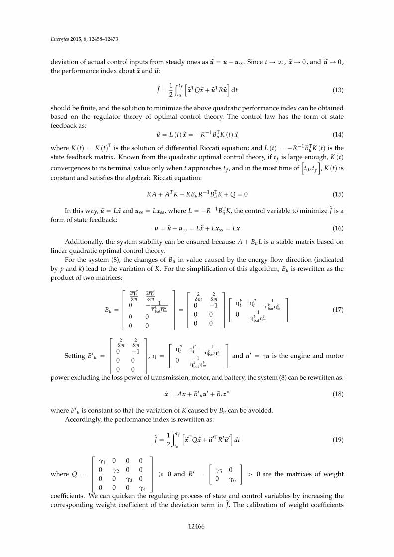
where K ptq “ K ptqT is the solution of differential Riccati equation; and L ptq “ ´R´1BTu K ptq is the
state feedback matrix. Known from the quadratic optimal control theory, if t f is large enough, K ptq
convergences to its terminal value only when t approaches t f , and in the most time of”
t0, t f
ı
, K ptq isconstant and satisfies the algebraic Riccati equation:
KA` ATK´ KBuR´1BTu K`Q “ 0 (15)
In this way, ru “ Lrx and uss “ Lxss, where L “ ´R´1BTu K, the control variable to minimize rJ is a
form of state feedback:u “ ru` uss “ Lrx` Lxss “ Lx (16)
Additionally, the system stability can be ensured because A ` BuL is a stable matrix based onlinear quadratic optimal control theory.
For the system (8), the changes of Bu in value caused by the energy flow direction (indicatedby p and k) lead to the variation of K. For the simplification of this algorithm, Bu is rewritten as theproduct of two matrices:
Bu “
»
—
—
—
—
–
2ηpt
δm2ηp
tδm
0 ´ 1ηk
batηkm
0 00 0
fi
ffi
ffi
ffi
ffi
fl
“
»
—
—
—
–
2δm
2δm
0 ´10 00 0
fi
ffi
ffi
ffi
fl
»
–
ηpt η
pt ´
1ηk
batηkm
0 1ηk
batηkm
fi
fl (17)
Setting B1u “
»
—
—
—
–
2δm
2δm
0 ´10 00 0
fi
ffi
ffi
ffi
fl
, η “
»
–
ηpt η
pt ´
1ηk
batηkm
0 1ηk
batηkm
fi
fl and u1 “ ηu is the engine and motor
power excluding the loss power of transmission, motor, and battery, the system (8) can be rewritten as:
.x “ Ax` B1uu1 ` Brz˚ (18)
where B1u is constant so that the variation of K caused by Bu can be avoided.Accordingly, the performance index is rewritten as:
rJ “12
ż t f
t0
”
rxTQrx` ru1TR1ru1ı
dt (19)
where Q “
»
—
—
—
–
γ1 0 0 00 γ2 0 00 0 γ3 00 0 0 γ4
fi
ffi
ffi
ffi
fl
ě 0 and R1 “
«
γ5 00 γ6
ff
ą 0 are the matrixes of weight
coefficients. We can quicken the regulating process of state and control variables by increasing thecorresponding weight coefficient of the deviation term in rJ. The calibration of weight coefficients
12466

Energies 2015, 8, 12458–12473
needs to ensure vehicle drivability, prevent large fluctuations of SOC, cut peaks and fill valleys ofengine power, and smooth the engine power to indirectly reduce fuel consumption.
For the optimal control problem of the system (18) and performance index (19), the solution hasthe form of Equation (16):
u1 “ L1x (20)
where L1 “ ´R1´1B1TuK1 is the matrix of state feedback and K1 satisfies:
K1A` ATK1 ´ K1B1uR1´1B1TuK1 `Q “ 0 (21)
Then, the engine power and motor power can be calculated by:
u “ η´1u1 “ ´η´1R1´1B1TuK1x (22)
where η “
»
–
ηpt η
pt ´
1ηk
batηkm
0 1ηk
batηkm
fi
fl changes with p and k, based on Preq and Pbat, respectively, i.e.,
p “
#
1, Preq ą 0
´1, Preq ď 0and k “
#
1, Pbat ą 0
´1, Pbat ď 0.
3.2. Two Control Modes
To further improve the fuel economy, two rules are designed to switch control modes (electricmode and hybrid mode) based on Preq for avoiding inefficient engine operation. The selection ofa switch point between the two control modes is combined with engine characteristics, vehicleparameters, and the principle of benefiting fuel economy. In this paper, the switch point is Preq “ P0,which is decided by comparing the energy conversion efficiency of a vehicle propelled separately byan engine and a motor. That is, when Preq “ P0, the efficiency of vehicle propelled solely by an engineis equal to the product of the efficiency of a vehicle propelled solely by a motor and the efficiencyof the battery charged by an engine [38]. The two control modes are realized by choosing differentweight coefficients of the quadratic performance index as follows:
(1) If Preq ď P0: the battery should provide the total driving power to avoid inefficient engineoperation or recover the braking energy that will be stored in the battery. Thus, we should set γ5 Ñ8
to make Pice approach to zero, and γ2 “ 0, γ4 “ 0 to temporarily not consider the constraint of SOCunless SOC reaches the maximum or minimum value.
(2) If Preq ą P0: the engine and battery should provide requested power together. The batteryshares the driving energy to restrain fluctuations of Pice. Now the constraint of SOC should benecessarily involved in the performance index for battery energy sustainability.
In general, the weight coefficients of two control modes can be calibrated by a test, where thedesired SOC is 0.7 and the desired vehicle velocity line is shown in Figure 6. In the calibration,to tune the weight coefficients of Q is similar to design a proportional integral (PI) controller: γ1
and γ2 correspond to proportional gains, γ3 and γ4 correspond to integral gains. In other words,increasing γ1 and γ3 results in faster response and smaller tracking errors of v, but paying the priceof larger fluctuations of SOC and more power provided by the engine and motor that may exceedtheir feasible bounds. Similarly, increasing γ2 and γ4 quickens the response of SOC and maintainsSOC nearer to 0.7 with a little influence on trajectories of v, Pice and Pess, but weakens the bufferingeffect of the battery. Additionally, the fluctuations ranges of Pice (or Pess) can be restricted within thefeasible bounds by appropriately increasing γ5 (or γ6) with a slight increment of tracking errors of v.According to the above changing laws about the control effect over weight coefficients, we can tunethe weight coefficients of two control modes by compromising between the tracking errors of statesand fluctuation ranges of control variables until obtaining a relatively better result of vehicle velocity
12467

Energies 2015, 8, 12458–12473
error, final SOC, and fuel economy. In this paper, the calibrated weight coefficients and correspondingK1 and L1 are given in Table 2. The test results with above weight coefficients are shown in Figure 6.
Table 2. Weight coefficients and state feedback matrixes of two rules.
Operationalcondition Weight coefficients K
1
L1
Preq ď P0
Q1 “
»
—
—
–
109 0 0 00 0 0 00 0 4ˆ 1010 00 0 0 0
fi
ffi
ffi
fl
R11 “„
1020 00 40
K11 “
»
—
—
–
2.36ˆ 108 0 ´8.95ˆ 108 00 0 0 0
´8.95ˆ 108 0 1.06ˆ 1010 00 0 0 0
fi
ffi
ffi
fl
L11 “„
0 0 0 0´8337.19 0 3.16ˆ 104 0
Preq ą P0
Q2 “
»
—
—
–
109 0 0 00 10´8 0 00 0 4ˆ 1010 00 0 0 5ˆ 10´7
fi
ffi
ffi
fl
R12 “„
80 00 80
K12 “
»
—
—
–
2.36ˆ 108 598.77 ´8.95ˆ 108 ´3.17598.77 1.69 ´16.32 ´0.0089
´8.95ˆ 108 ´16.32 1.06ˆ 1010 0.10´3.17 ´0.0089 0.10 9ˆ 10´5
fi
ffi
ffi
fl
L12 “„
´4172.34 ´0.01 1.58ˆ 104 5.59ˆ 10´5
´4164.85 0.01 1.58ˆ 104 ´5.59ˆ 10´5
Actually, the more the detailed operational conditions are divided, the better the control effect ofQPIS is obtained, but much more complex algorithms are needed, which will weaken the adaptabilityof QPIS. Eventually, the concrete form of QPIS is:
#
u1 “ ´η´1R1´1
1 B1TuK11x, Preq ď P0
u2 “ ´η´1R1´1
2 B1TuK12x, Preq ą P0(23)
The control system of QPIS is shown in Figure 7. It can be observed that the control variables ofQPIS are simple linear functions of current system states x without future driving conditions. Thisinteresting feature makes QPIS simply structured and particularly suitable for real-time optimizationcontrol. Furthermore, u1, and u2 are switched based on Preq, which is the sum of Pice and Pess
calculated by QPIS. To avoid frequent switches of control functions at switch points, we necessarilyadd a hysteresis loop when Preq “ P0, of which the switch on and off points are Pon “ 8 kW andPo f f “ 2 kW, respectively, and the engine power and motor power of u1 and u2 are limited in theirrespective feasible ranges.Energies 2015, 8 14
(m/s
)v
(kW
)ic
eP
(kW
)es
sP
Figure 6. Test results of calibrated weight coefficients
Actually, the more the detailed operational conditions are divided, the better the control effect of
QPIS is obtained, but much more complex algorithms are needed, which will weaken the adaptability
of QPIS. Eventually, the concrete form of QPIS is:
1 1 T1 1 1 req 0
1 1 T2 2 2 req 0
η ,
η ,
u
u
R B K P P
R B K P P
u x
u x (23)
The control system of QPIS is shown in Figure 7. It can be observed that the control variables of
QPIS are simple linear functions of current system states x and commands *z without future driving
conditions. This interesting feature makes QPIS simply structured and particularly suitable for real-time optimization control. Furthermore, 1u , and 2u are switched based on reqP , which is the sum
of iceP and essP calculated by QPIS. To avoid frequent switches of control functions at switch points,
we necessarily add a hysteresis loop when req 0P P , of which the switch on and off points are
8 kWonP and 2 kWoffP , respectively, and the engine power and motor power of 1u and 2u are
limited in their respective feasible ranges.
Figure 6. Test results of calibrated weight coefficients.
12468
Energies 2015, 8, 12458–12473Energies 2015, 8 15
Vehicle control unit
Engine MAP(Fig. 2)
Motor MAP(Fig. 4)
Battery model(Equation (4))
QPIS(Equation (23))
Vehicle model (Equation (3))
* 2( )v
*SOCE
2 SOCx E
21x v
*iceP*
essP* ,iceT *
ice Torque coupler and CVT
*batP
CVT ratio1
s
1
s
3x
4x
Mechanical/electrical connection
Information flow direction
* *,ess essT
*ice
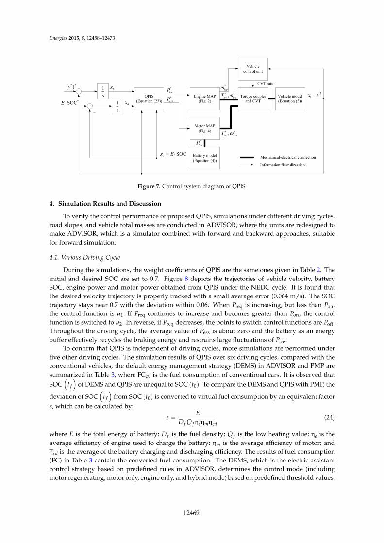
Figure 7. Control system diagram of QPIS.
4. Simulation Results and Discussion
To verify the control performance of proposed QPIS, simulations under different driving cycles,
road slopes, and vehicle total masses are conducted in ADVISOR, where the units are redesigned to
make ADVISOR, which is a simulator combined with forward and backward approaches, suitable for
forward simulation.
4.1. Various Driving Cycle
During the simulations, the weight coefficients of QPIS are the same ones given in Table 2. The
initial and desired SOC are set to 0.7. Figure 8 depicts the trajectories of vehicle velocity, battery SOC,
engine power and motor power obtained from QPIS under the NEDC cycle. It is found that the desired velocity trajectory is properly tracked with a small average error ev (0.064 m/s). The SOC trajectory
stays near 0.7 with the deviation within 0.06. When reqP is increasing, but less than onP , the control
function is 1u . If reqP continues to increase and becomes greater than onP , the control function is
switched to 2u . In reverse, if reqP decreases, the points to switch control functions are offP .
Throughout the driving cycle, the average value of essP is about zero and the battery as an energy
buffer effectively recycles the braking energy and restrains large fluctuations of iceP .
Figure 7. Control system diagram of QPIS.
4. Simulation Results and Discussion
To verify the control performance of proposed QPIS, simulations under different driving cycles,road slopes, and vehicle total masses are conducted in ADVISOR, where the units are redesigned tomake ADVISOR, which is a simulator combined with forward and backward approaches, suitablefor forward simulation.
4.1. Various Driving Cycle
During the simulations, the weight coefficients of QPIS are the same ones given in Table 2. Theinitial and desired SOC are set to 0.7. Figure 8 depicts the trajectories of vehicle velocity, batterySOC, engine power and motor power obtained from QPIS under the NEDC cycle. It is found thatthe desired velocity trajectory is properly tracked with a small average error (0.064 m/s). The SOCtrajectory stays near 0.7 with the deviation within 0.06. When Preq is increasing, but less than Pon,the control function is u1. If Preq continues to increase and becomes greater than Pon, the controlfunction is switched to u2. In reverse, if Preq decreases, the points to switch control functions are Poff.Throughout the driving cycle, the average value of Pess is about zero and the battery as an energybuffer effectively recycles the braking energy and restrains large fluctuations of Pice.
To confirm that QPIS is independent of driving cycles, more simulations are performed underfive other driving cycles. The simulation results of QPIS over six driving cycles, compared with theconventional vehicles, the default energy management strategy (DEMS) in ADVISOR and PMP aresummarized in Table 3, where FCcv is the fuel consumption of conventional cars. It is observed thatSOC
´
t f
¯
of DEMS and QPIS are unequal to SOC pt0q. To compare the DEMS and QPIS with PMP, the
deviation of SOC´
t f
¯
from SOC pt0q is converted to virtual fuel consumption by an equivalent factors, which can be calculated by:
s “E
D f Q fηeηmηcd(24)
where E is the total energy of battery; D f is the fuel density; Q f is the low heating value; ηe is theaverage efficiency of engine used to charge the battery; ηm is the average efficiency of motor; andηcd is the average of the battery charging and discharging efficiency. The results of fuel consumption(FC) in Table 3 contain the converted fuel consumption. The DEMS, which is the electric assistantcontrol strategy based on predefined rules in ADVISOR, determines the control mode (includingmotor regenerating, motor only, engine only, and hybrid mode) based on predefined threshold values,
12469

Energies 2015, 8, 12458–12473
as well as actual states and driving commands. It is suitable for real-time control, but with limitedfuel economy.Energies 2015, 8 16
(m/s
)v
(kW
)ic
eP
2u
1u
2u1u
(kW
)es
sP
Figure 8. Simulation results of QPIS over NEDC cycle in ADVISOR
To confirm that QPIS is independent of driving cycles, more simulations are performed under five
other driving cycles. The simulation results of QPIS over six driving cycles, compared with the
conventional vehicles, the default energy management strategy (DEMS) in ADVISOR and PMP are
summarized in Table 3, where FCcv is the fuel consumption of conventional cars. It is observed that
SOC ft of DEMS and QPIS are unequal to 0SOC t . To compare the DEMS and QPIS with PMP,
the deviation of SOC ft from 0SOC t is converted to virtual fuel consumption by an equivalent
factor s , which can be calculated by:
f f e m cd
Es
D Q
(24)
where E is the total energy of battery; fD is the fuel density; fQ is the low heating value; e is the
average efficiency of engine used to charge the battery; m is the average efficiency of motor; and cd
is the average of the battery charging and discharging efficiency. The results of fuel consumption (FC)
in Table 3 contain the converted fuel consumption. The DEMS, which is the electric assistant control
strategy based on predefined rules in ADVISOR, determines the control mode (including motor
Figure 8. Simulation results of QPIS over NEDC cycle in ADVISOR.
Table 3. Simulation results of DEMS, PMP, and QPIS over various driving cycles in ADVISOR.
Driving cycle FCcv(L/100 km)
DEMS PMP QPIS
FC(L/100 km) SOC (t f ) FC
(L/100 km) SOC (t f ) λ(g/J) FC(L/100 km) SOC (t f )
CSHVR 6.9956 5.1110 0.6421 3.4589 0.6989 ´6.5929ˆ 10´5 3.6588 0.7017UDDS 6.2529 5.2505 0.6423 3.8370 0.6935 ´6.4840ˆ 10´5 3.8616 0.7184
WVUINTER 4.9847 4.5921 0.6633 3.9466 0.6844 ´7.0056ˆ 10´5 4.1855 0.6905FTP 6.1682 5.1168 0.6601 3.8318 0.6998 ´6.4466ˆ 10´5 3.9549 0.6853
NEDC 6.3946 5.3694 0.6667 4.0313 0.6867 ´6.8726ˆ 10´5 4.1185 0.6975INDIA_URBAN 6.5888 5.2862 0.6401 3.4747 0.6950 ´6.7667ˆ 10´5 3.5842 0.7220
It is amazingly found in Table 3 that even if driving cycles are changed, the control effect of QPISwith the same group of weight coefficients remains as excellent as the results under NEDC. Comparedto conventional cars, the three EMSes significantly reduce the fuel consumption. Especially, theQPIS and PMP achieve higher fuel economy than DEMS. More importantly, the fuel consumptionimprovement of QPIS over six driving cycles is quite close (just slightly lower, i.e., less than 4.8% atworst and 0.4% at best) to that of PMP. It is demonstrated that QPIS, which inherits the advantages ofreal-time performance of DEMS and the improvement in fuel economy of PMP, can be applied to thepower assignment for HEVs even if the future driving cycle is unknown.
4.2. Various Road Slopes and Vehicle Total Masses
The influences of θ and m on the control effect of QPIS are involved in this section becausevehicles usually run on slopes and the vehicle total mass may change in practice. In ADVISOR, θ canbe easily added to a driving cycle as a function of distance and m can be easily changed by settingthe vehicle parameter. Tables 4 and 5 show the results of DEMS, QPIS, and PMP when the HEV runs
12470
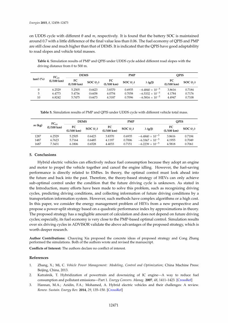
Energies 2015, 8, 12458–12473
on UDDS cycle with different θ and m, respectively. It is found that the battery SOC is maintainedaround 0.7 with a little difference of the final value less than 0.06. The fuel economy of QPIS and PMPare still close and much higher than that of DEMS. It is indicated that the QPIS have good adaptabilityto road slopes and vehicle total masses.
Table 4. Simulation results of PMP and QPIS under UDDS cycle added different road slopes with thedriving distance from 0 to 500 m.
tanθ (%) FCcv(L/100 km)
DEMS PMP QPIS
FC(L/100 km)
SOC (t f ) FC(L/100 km)
SOC (t f ) λ (g/J) FC(L/100 km)
SOC (t f )
0 6.2529 5.2505 0.6423 3.8370 0.6935 ´6.4840 ˆ 10´5 3.8616 0.71845 6.4773 5.4736 0.6458 4.0754 0.7058 ´6.5332 ˆ 10´5 4.1784 0.7176
10 6.8242 5.7475 0.6473 4.3187 0.7096 ´6.5816 ˆ 10´5 4.4947 0.7108
Table 5. Simulation results of PMP and QPIS under UDDS cycle with different vehicle total mass.
m (kg) FCcv(L/100 km)
DEMS PMP QPIS
FC(L/100 km)
SOC (t f ) FC(L/100 km)
SOC (t f ) λ (g/J) FC(L/100 km)
SOC (t f )
1287 6.2529 5.2505 0.6423 3.8370 0.6935 ´6.4840 ˆ 10´5 3.8616 0.71841487 6.7623 5.7164 0.6485 4.1197 0.7006 ´6.3367 ˆ 10´5 4.1955 0.70491687 7.3431 6.1806 0.6528 4.4033 0.7151 ´6.2239 ˆ 10´5 4.5818 0.7061
5. Conclusions
Hybrid electric vehicles can effectively reduce fuel consumption because they adopt an engineand motor to propel the vehicle together and cancel the engine idling. However, the fuel-savingperformance is directly related to EMSes. In theory, the optimal control must look ahead intothe future and back into the past. Therefore, the theory-based strategy of HEVs can only achievesub-optimal control under the condition that the future driving cycle is unknown. As stated inthe Introduction, many efforts have been made to solve this problem, such as recognizing drivingcycles, predicting driving conditions, and collecting information of future driving conditions by atransportation information system. However, such methods have complex algorithms or a high cost.In this paper, we consider the energy management problem of HEVs from a new perspective andpropose a power-split strategy based on a quadratic performance index by approximations in theory.The proposed strategy has a negligible amount of calculation and does not depend on future drivingcycles; especially, its fuel economy is very close to the PMP-based optimal control. Simulation resultsover six driving cycles in ADVISOR validate the above advantages of the proposed strategy, which isworth deeper research.
Author Contributions: Chaoying Xia proposed the concrete ideas of proposed strategy and Cong Zhangperformed the simulations. Both of the authors wrote and revised the manuscript.
Conflicts of Interest: The authors declare no conflict of interest.
References
1. Zhang, X.; Mi, C. Vehicle Power Management: Modeling, Control and Optimization; China Machine Press:Beijing, China, 2013.
2. Katrašnik, T. Hybridization of powertrain and downsizing of IC engine—A way to reduce fuelconsumption and pollutant emissions—Part 1. Energy Convers. Manag. 2007, 48, 1411–1423. [CrossRef]
3. Hannan, M.A.; Azidin, F.A.; Mohamed, A. Hybrid electric vehicles and their challenges: A review.Renew. Sustain. Energy Rev. 2014, 29, 135–150. [CrossRef]
12471

Energies 2015, 8, 12458–12473
4. Bayindir, K.C.; Gozukucuk, M.A.; Teke, A. A comprehensive overview of hybrid electric vehicle:Powertrain configurations, powertrain control techniques and electronic control units. Energy Convers.Manag. 2011, 52, 1305–1313. [CrossRef]
5. Jalil, N.; Kheir, N.A.; Salman, M. A Rule-based energy management strategy for a series hybrid vehicle.In Proceedings of the American Control Conference, Albuquerque, NM, USA, 4–6 June 1997.
6. Banvait, H.; Anwar, S.; Chen, Y. A rule-based energy management strategy for plug-in hybrid electricvehicle. In Proceedings of the American Control Conference, St. Louis, MO, USA, 10–12 June 2009.
7. Cipek, M.; Pavkovic, D.; Petric, J. A control-oriented simulation model of a power-split hybrid electricvehicle. Appl. Energy 2013, 101, 121–133. [CrossRef]
8. Liu, S.H.; Du, C.Q.; Yan, F.W.; Wan, J.; Li, Z.; Luo, Y. A rule-based energy management strategy for a NewBSG hybrid electric vehicle. In Proceedings of the Global Congress on Intelligent Systems, Wuhan, China,6–8 November 2012.
9. Schouten, N.J.; Salman, M.A.; Kheir, N.A. Fuzzy logic control for parallel hybrid vehicles. IEEE Trans.Control Syst. Technol. 2002, 10, 460–468. [CrossRef]
10. Duan, Y.B.; Zhang, W.G.; Huang, Z. Simulation of fuzzy logic control strategy for HEV. Chin. Intern.Combust. Engine Eng. 2003, 24, 66–69.
11. Zhao, G.Y.; Du, Z.Y.; Du, Z.Y.; Chen, W.Q. Energy management strategy for series hybrid electric vehicle.J. Northeast. Univ. Natl. Sci. 2013, 34, 583–587.
12. Wu, J.; Zhang, C.H.; Cui, N.X. Fuzzy energy management strategy of parallel hybrid electric vehicle basedon particle swarm optimization. Control Decis. 2008, 23, 46–50.
13. Zhou, M.L.; Lu, D.K.; Li, W.M.; Xu, H.F. Optimized fuzzy logic control strategy for parallel hybrid electricvehicle based on genetic algorithm. Appl. Mech. Mater. 2013, 274, 345–349. [CrossRef]
14. Murphey, Y.L.; Chen, Z.H.; Kiliaris, L.; Masrur, M.A. Intelligent power management in a vehicular systemwith multiple power sources. J. Power Sources 2011, 196, 835–846. [CrossRef]
15. Wu, J.; Zhang, C.H.; Cui, N.X. Fuzzy energy management strategy for a hybrid electric vehicle based ondriving cycle recognition. Int. J. Automot. Technol. 2012, 13, 1159–1167. [CrossRef]
16. Tian, Y.; Zhang, X.; Zhang, L. Fuzzy control strategy for hybrid electric vehicle based on neural networkidentification of driving conditions. Control Theory Appl. 2011, 28, 363–369.
17. Wang, R.; Lukic, S.M. Dynamic programming technique in hybrid electric vehicle optimization.In Proceedings of the IEEE International Electric Vehicle Conference, Greenville, SC, USA, 4–8 March 2012.
18. Perez, L.V.; Bossio, G.R.; Moitre, D.; Garcia, G.O. Optimization of power management in an hybrid electricvehicle using dynamic programming. Math. Comput. Simul. 2006, 73, 244–254. [CrossRef]
19. Patil, R.M.; Filipi, Z.; Fathy, H.K. Comparison of supervisory control strategies for series plug-in hybridelectric vehicle powertrains through dynamic programming. IEEE Trans. Control Syst. Technol. 2014, 22,502–509. [CrossRef]
20. Zou, Y.; Sun, F.C.; Zhang, C.N.; Li, J.Q. Optimal energy management strategy for hybrid electric trackedvehicles. Int. J. Veh. Des. 2012, 58, 307–324. [CrossRef]
21. Pisu, P.; Rizzoni, G. A comparative study of supervisory control strategies for hybrid electric vehicles.IEEE Trans. Control Syst. Technol. 2007, 15, 506–518. [CrossRef]
22. Kum, D.; Peng, H.; Bucknor, N.K. Supervisory control of parallel hybrid electric vehicles for fuel andemission reduction. J. Dyn. Syst. Meas. Control 2011, 133, 061010. [CrossRef]
23. Bianchi, D.; Rolando, L.; Serrao, L.; Onori, S.; Rizzoni, G.; Al-Khayat, N.; Hsieh, T.M.; Kang, P.J.A rule-based strategy for a series/parallel hybrid electric vehicle: An approach based on dynamicprogramming. In Proceedings of the Dynamic Systems and Control Conference, Cambridge, MA, USA,12–15 September 2010.
24. Zou, Y.; Hou, S.J.; Li, D.G.; Wei, G.; Hu, X.S. Optimal energy control strategy design for a hybrid electricvehicle. Discret. Dyn. Nat. Soc. 2013. [CrossRef]
25. Lin, C.C.; Peng, H.; Grizzle, J.W. A stochastic control strategy for hybrid electric vehicles. In Proceedings ofthe American Control Conference, Boston, MA, USA, 30 June´2 July 2004.
26. Lin, X.Y.; Sun, D.Y.; Yin, Y.L.; Hao, Y.Z. The energy management strategy for a series-parallel hybrid electricbus based on stochastic dynamic programming. Automot. Eng. 2012, 34, 830–835, 858.
12472
Energies 2015, 8, 12458–12473
27. Borhan, H.; Vahidi, A.; Phillips, A.M.; Kuang, M.L.; Kolmanovsky, I.V.; Cairano, S.D. MPC-based energymanagement of a power-split hybrid electric vehicle. IEEE Trans. Control Syst. Technol. 2012, 20, 593–603.[CrossRef]
28. Donateo, T.; Pacella, D.; Laforgia, D. A method for the prediction of future driving conditions and for theenergy management optimization of a hybrid electric vehicle. Int. J. Veh. Des. 2012, 58, 111–133. [CrossRef]
29. Van Keulen, T.; de Jager, B.; Serrarens, A.; Steinbuch, M. Optimal energy management in hybrid electrictrucks using route information. Oil Gas Sci. Technol. 2010, 65, 103–113. [CrossRef]
30. Kim, N.; Rousseau, A.; Lee, D. A jump condition of PMP-based control for PHEVs. J. Power Sources 2011,196, 10380–10386. [CrossRef]
31. Zou, Y.; Liu, T.; Sun, F.; Peng, H. Comparative study of dynamic programming and Pontryagin’s minimumprinciple on energy management for a parallel hybrid electric vehicle. Energies 2013, 6, 2305–2318.
32. Kim, N.; Cha, S.; Peng, H. Optimal control of hybrid electric vehicles based on Pontryagin’s minimumprinciple. IEEE Trans. Control Syst. Technol. 2011, 19, 1279–1287.
33. Serrao, L.; Onori, S.; Rizzoni, G. ECMS as a realization of Pontryagin's minimum principle for HEV control.In Proceedings of the American Control Conference, St. Louis, MO, USA, 10–12 June 2009.
34. Paganelli, G.; Delprat, S.; Guerra, T.M.; Rimaux, J.; Santin, J.J. Equivalent consumption minimizationstrategy for parallel hybrid powertrains. In Proceedings of the IEEE Vehicular Technology Conference,Birmingham, AL, USA, 6–9 May 2002.
35. Kim, N.; Cha, S.W.; Peng, H. Optimal equivalent fuel consumption for hybrid electric vehicles. IEEE Trans.Control Syst. Technol. 2012, 20, 817–825.
36. Gurkaynak, Y.; Khaligh, A.; Emadi, A. Neural adaptive control strategy for hybrid electric vehicles withparallel powertrain. In Proceedings of the IEEE Vehicle Power and Propulsion Conference, Lille, France,1–3 September 2010.
37. Musardo, C.; Rizzoni, G.; Staccia, B. A-ECMS: An adaptive algorithm for hybrid electric vehicles energymanagement. In Proceedings of the 44th IEEE Conference on Decision and Control, and the EuropeanControl Conference, Seville, Spain, 12–15 December 2005.
38. Wu, J. Optimization of Energy Management Strategy for Parallel Hybrid Electric Vehicle. Ph.D. Thesis,Department of Control Theory Control Engineering, Shandong University, Shandong, China, 2008.
© 2015 by the authors; licensee MDPI, Basel, Switzerland. This article is an openaccess article distributed under the terms and conditions of the Creative Commons byAttribution (CC-BY) license (http://creativecommons.org/licenses/by/4.0/).
12473