Embed Size (px)
Citation preview

Living StandardsMeasurement StudyWorking Paper No. 86
Poverty and Inequality during Unorthodox Adjustment
The Case of Peru, 1985-90
Pub
lic D
iscl
osur
e A
utho
rized
Pub
lic D
iscl
osur
e A
utho
rized
Pub
lic D
iscl
osur
e A
utho
rized
Pub
lic D
iscl
osur
e A
utho
rized
Pub
lic D
iscl
osur
e A
utho
rized
Pub
lic D
iscl
osur
e A
utho
rized
Pub
lic D
iscl
osur
e A
utho
rized
Pub
lic D
iscl
osur
e A
utho
rized
LSMS Working Papers
No. 15 Measuring Health as a Component of Living Standards
No. 16 Procedures for Collecting and Analyzing Mortality Data in LSMS
No. 17 The Labor Market and Social Accounting: A Framework of Data Presentation
No. 18 Time Use Data and the Living Standards Measurement Study
No. 19 The Conceptual Basis of Measures of Household Welfare and Their Implied Survey Data Requirements
No. 20 Statistical Experimentation for Household Surveys: Two Case Studies of Hong Kong
No. 21 The Collection of Price Data for the Measurement of Living Standards
No. 22 Household Expenditure Surveys: Some Methodological Issues
No. 23 Collecting Panel Data in Developing Countries: Does It Make Sense?
No. 24 Measuring and Analyzing Levels of Living in Developing Countries: An Annotated Questionnaire
No. 25 The Demand for Urban Housing in the Ivory Coast
No. 26 The C6te d'Ivoire Living Standards Survey: Design and Implementation
No. 27 The Role of Employment and Earnings in Analyzing Levels of Living: A General Methodology withApplications to Malaysia and Thailand
No. 28 Analysis of Household Expenditures
No. 29 The Distribution of Welfare in Cdte d'Ivoire in 1985
No. 30 Quality, Quantity, and Spatial Variation of Price: Estimating Price Elasticities from Cross-SectionalData
No. 31 Financing the Health Sector in Peru
No. 32 Informal Sector, Labor Markets, and Returns to Education in Peru
No. 33 Wage Determinants in COte d'Ivoire
No. 34 Guidelines for Adapting the LSMS Living Standards Questionnaires to Local Conditions
No. 35 The Demand for Medical Care in Developing Countries: Quantity Rationing in Rural C6te d'Ivoire
No. 36 Labor Market Activity in C6te d'Ivoire and Peru
No. 37 Health Care Financing and the Demand for Medical Care
No. 38 Wage Detenninants and School Attainment among Men in Peru
No. 39 The Allocation of Goods within the Household: Adults, Children, and Gender
No. 40 The Effects of Household and Community Characteristics on the Nutrition of Preschool Children:Evidence from Rural Cate d'Ivoire
No. 41 Public-Private Sector Wage Differentials in Peru, 1985-86
No. 42 The Distribution of Welfare in Peru in 1985-86
No. 43 Profits from Self-Employment: A Case Study of COte d'Ivoire
No. 44 The Living Standards Survey and Price Policy Reform: A Study of Cocoa and Coffee Production inCdte d'Ivoire
No. 45 Measuring the Willingness to Payfor Social Services in Developing Countries
No. 46 Nonagricultural Family Enterprises in Cate d'Ivoire: A Descriptive Analysis
No. 47 The Poor during Adjustment: A Case Study of C6te d'Ivoire
No. 48 Confronting Poverty in Developing Countries: Definitions, Information, and Policies
No. 49 Sample Designs for the Living Standards Surveys in Ghana and Mauritania/Plans de sondagepour les enquetes sur le niveau de vie au Ghana et en Mauritanie
No. 50 Food Subsidies: A Case Study of Price Reform in Morocco (also in French, 50F)
(List continues on the inside back cover)

Poverty and Inequality during Unorthodox Adjustment
The Case of Peru, 1985-90
I

The Living Standards Measurement Study
The Living Standards Measurement Study (LsMs) was established by theWorld Bank in 1980 to explore ways of improving the type and quality of house-hold data collected by statistical offices in developing countries. Its goal is to fosterincreased use of household data as a basis for policy decisionmaking. Specifically,the LsMS is worldng to develop new methods to monitor progress in raising levelsof living, to identify the consequences for households of past and proposed gov-ernment policies, and to improve communcations between survey statisticians, an-alysts, and policymakers.
The LSMS Working Paper senes was started to disseminate intermediate prod-ucts from the LSMS. Publications in the series include critical surveys covering dif-ferent aspects Df the ISMS data collection program and reports on improvedmethodologies for using Living Standards Survey (TSS) data. More recent publica-tions recommend specific survey, questionnaire, and data processing designs, anddemonstrate the breadth of policy analysis that can be carried out using LSS data.

LSMS Working PaperNumber 86
Poverty and Inequality during Unorthodox Adjustment
The Case of Peru, 1985-90
Paul Glewwe and Gillette Hall
The World BankWashington, D.C.
Copyright 0 1992The International Bank for Reconstructionand Development/THE WORLD BANK1818 H Street, N.W.Washington, D.C. 20433, U.S.A.
All rights reservedManufactured in the United States of AmericaFirst printing February 1992
To present the results of the Living Standards Measurement Study with the least possible delay, thetypescript of this paper has not been prepared in accordance with the procedures appropriate to formalprinted texts, and the World Bank accepts no responsibility for errors.
The findings, interpretations, and conclusions expressed in this paper are entirely those of the author(s)and should not be attributed in any manner to the World Bank, to its affiliated organizations, or to membersof its Board of Executive Directors or the countries they represent. The World Bank does not guarantee theaccuracy of the data included in this publication and accepts no responsibility whatsoever for anyconsequence of their use. Any maps that accompany the text have been prepared solely for the convenienceof readers; the designations and presentation of material in them do not imply the expression of anyopinion whatsoever on the part of the World Bank, its affiliates, or its Board or member countriesconcerning the legal status of any country, territory, city, or area or of the authorities thereof or concerningthe delimitation of its boundaries or its national affiliation.
The material in this publication is copyrighted. Requests for permission to reproduce portions of it shouldbe sent to the Office of the Publisher at the address shown in the copyright notice above. The World Bankencourages dissemination of its work and will normally give permission promptly and, when thereproduction is for noncommercial purposes, without asking a fee. Permission to photocopy portions forclassroom use is not required, though notification of such use having been made will be appreciated.
The complete backlist of publications from the World Bank is shown in the annual Index of Publications,which contains an alphabetical title list (with fuill ordering information) and indexes of subjects, authors,and countries and regions. The latest edition is available free of charge from the Distribution Unit, Office ofthe Publisher, Department F, The World Bank, 1818 H Street, N.W., Washington, D.C. 20433, U.S.A., or fromPublications, The World Bank, 66, avenue d'Iena, 75116 Paris, France.
ISSN: 02534517
Paul Glewwe is an economist in the Welfare and Human Resources Division of the Population andHuman Resources Department of the World Bank. Gillette Hall is a Ph.D. candidate at CambridgeUniversity in the Faculty of Economics.
Library of Congress Cataloging-in-Publication Data
Glewwe, Paul, 1958-Poverty and inequality during unorthodox adjustment: the case of
Peru, 1985-90 / Paul Glewwe and Gillette Hall.p. cm. - (Living standards measurement study, ISSN 0253-4517
86)Includes bibliographical references.ISBN 0-8213-2060-21. Poor-Peru-Lima. 2. Cost and standard of licing-Peru-Lima.
3. Consumption (Economics)-Peru-Lima. 4. Structural adjustment(Economic policy)-Peru. 5. Peru-Economic policy. I. Hall,Gillette, 1962- . II. Title. m. Series: LSMS working paper;no. 86.HC228.L5G58 1992339.4'7'098525-dc2O 92-239
CIP

ABSTRACT
This paper examines the change in poverty and inequality in Lima, Peru
between 1985-86 and 1990. The data employed are from the 1985-86 and 1990 Living
Standards Measurement Surveys. The results are presented in the context of the
"unorthodox" macroeconomic policies which were undertaken between those years by
the Peruvian government. However, no attempt is made to link specific
macroeconomic policies to welfare outcomes. The paper presents a descriptive
account of poverty and living conditions in Lima, and discusses some of the
implications of the findings for social investment programs. The major findings
are:
1. Between 1985-86 and 1990 the average household in Lima experienceda decline in per capita consumption of 55 percent.
2. Poverty, defined as the inability to cover the household's basicnutritional requirements, increased from 0.5% of the population in1985-86 to 17.3% in 1990.
3. The poorest 20% of the population, especially the poorest 10%,suffered the most, experiencing declines in consumption of more than60 percent.
4. Households headed by individuals with little or no educationexperienced greater declines in consumption than the bettereducated. Longer run social investment plans should prioritizeeducation.
5. The rate of unemployment increased significantly, and by 1990 hadbecome a distinct characteristic of the poor. Programs designed toincrease low-wage employment opportunities would be self-targeted tothe poorest households.
6. The provision of public services, particularly potable water andsewage services, deteriorated most significantly in the poorestareas of the city, among those who also suffered the greatestdeclines in per consumption. Public investment in public water andsanitation services is recommended in these areas.
7. Households headed by women are not found to have suffered greaterdeclines in per capita consumption than male headed households.
8. Recently settled "pueblos jovenes" are not disproportionatelypopulated by poor families. The poorest families are well-distributed throughout the three poorest regions of the city.
- v -

ACKNOWLEDGEMENTS
We would like to thank Kalpana Mehra for excellent research assistance.
Useful comments on earlier versions of this paper were given by Karen Cavenaugh,
Emmanuel Jimenez, Polly Jones, Ricardo Lago, Izumi Ohno, Francisco Sagasti and
Jacques van der Gaag. We are very grateful to the staff of Cuanto, S.A., Lima,
Peru, whose collaboration made possible the LSMS survey work in 1990.
- vi -

FOREWORD
The World Bank's structural adjustment policies have been criticized in
recent years for failure to adequately protect the living standards of the poor.
The real issue is whether alternative policies could have done a better job of
protecting the poor while reviving economic growth. This paper examines an
alternative set of policies adopted in Peru from 1985 to 1990, and the findings
are quite sobering; not only did the economy as a whole deteriorate, but the
policies also failed to protect the poor.
This paper is part of a broader program of research in the Population and
Human Resources (PHR) Department on the extent of poverty in developing countries
and on policies to reduce poverty. This research program is located in the
Welfare and Human Resources Division. The data used here are from the Peru
Living Standards Survey, which is one of the Living Standards Measurement Study
(LSMS) household surveys which the World Bank has implemented in many developing
countries. Aside from the findings in this study for Peru, one of the other
objectives of this and similar work using LSMS data is to demonstrate the need
for and usefulness of household data collection efforts in other developing
countries.
Ann 0. HamiltonDirector
Population and Human Resources Department
- vii -


TABLE OF CONTENTS
I. Introduction . . . . . . . . . . . . . . . . . . . . . . . . . . . . 1
II. Peruvian Economic Policy, 1980-90 ........ ... 3
The Peruvian Economy in the Early 1980s . . . . . . . . . . . . . . 3The Formulation of Peruvian Economic Policy, 1985-90 . . . . . . . 4
III. Living Standards Data and Their Use in Assessing Household Welfare . 8
The Peru Living Standards Surveys . . . . . . . . . . . . . . . . . 8Using the LSMS Data to Construct an Indicator ofHousehold Welfare ....................... . 10
IV. Changes in the Distribution of Consumption from 1985-86 to 1990 . . . 15
Changes in the Overall Distribution of Consumption Expenditures . . 15Changes in Consumption Expenditures by Areas within Lima . . . . . 18Changes in Consumption Expenditures by Head of Household
Characteristics ........................ . 20Other Indicators of Living Standards . . . . . . . . . . . . . . . 26
V. Poverty in Lima from 1985-86 to 1990 ... . . . . . . . . . . . . . 38
Measuring the Incidence of Poverty in Lima . . . . . . . . . . . . 38Implications of the Study for Social Program Targeting . . . . . . 42
VI. Conclusion . . . . . . . . . . . . . . . . . . . . . . . . . . . . . 48
VII. Appendices
Survey Format, 1985-86 and 1990 . . . . . . . . . . . . . . . . . . 51Construction of Price Deflators . . . . . . . . . . . . . . . . . . 52Calculation of Household Consumption . . . . . . . . . . . . . . . 58Changes in Real Expenditures in Lima, 1985-86 to 1990, byExpenditure Decile, Unadjusted . . . . . . . . . . . . . . . . . 60
Use of Household-Specific Price Deflators . . . . . . . . . . . . . 61List of Geographic Areas . . . . . . . . . . . . . . . . . . . . . 65
VIII. References . . . . . . . . . . . . ... . . . . . . . . . . . . . . . 67
LIST OF TABLES
Table 1. Index of Basic Indicators, Peru: 1980, 1985, and 1990 . . . . 6
Table 2. Mean Monthly Consumption Expenditures in Lima,1985-86 and 1990 . . . . . . . . . . . . . . . . . . . . . . . 13
Table 3. Changes in Real Expenditures in Lima, 1985-86 to 1990,by Expenditure Decile . . . . . . . . . . . . . . . . . . . . . 16
Table 4. Changes in Real Monthly Expenditures Per Capita,1985-86 to 1990, by Area . . . . . . . . . . . . . . . . . . . 19
Table 5. Changes in Per Capita Monthly Expenditures by Characteristicsof Household Head, All Lima . . . . . . . . . . . . . . . . . . 21
- ix -

Table 6. Changes in Per Capita Monthly Expenditures by Characteristicsof Household Head, Old Lima ................. . 22
Table 7. Distribution of Population by Characteristics of HouseholdHeads, by Quintile, All Lima, 1985-86 . . . . . . . . . . . . . 26
Table 8. Distribution of Population by Characteristics of HouseholdHeads, by Quintile, All Lima, 1990 . . . . . . . . . . . . . . 27
Table 9. Characteristics of Household Heads by Quintile, Old Lima, 1990 28
Table 10. Distribution of Population by Housing Characteristics,All Lima 1985-86, by Quintile ... . . . . . . . . . . . . . . 29
Table 11. Housing Characteristics, All Lima, 1990, by ExpenditureQuintile . . . . . . . . . . . . . . . . . . . . . . . . . . . 30
Table 12. Distribution of Population by Housing Characteristics,All Lima, 1985-86, by Area ................. . 33
Table 13. Distribution of Population by Housing Characteristics,All Lima, 1990, by Area ................... . 34
Table 14. Change in Distribution of Durable Good Ownership,1985-86 to 1990, 'All Lima', by Quintile . . . . . . . . . . . 36
Table 15. Change in Distribution of Durable Good Ownership,1985-86 to 1990, 'All Lima', by Area . . . . . . . . . . . . . 37
Table 16. Poverty Lines Based on Monthly Real Expenditures . . . . . . . 39
Table 17. Incidence of Poverty in All Lima by Area, 1985-86 and 1990 . 42
x

I. Introduction
The 1980s were not a prosperous decade for most developing countries. The
majority of these countries experienced periods of economic stagnation, if not
outright decline. For many of these countries, adapting to the new, less
promising external environment has required a shift in macroeconomic policies.
For most countries, this shift has entailed the implementation of structural
adjustment programs recommended and partially financed by the World Bank. A few,
however, have experimented with alternative programs in the hopes of reducing the
perceived economic and social costs of structural adjustment.
World Bank stabilization programs have recently been the topic of much
evaluation and discussion in terms of their social and distributional
consequences (Addison and Demery, 1985, 1986; Cornia, Jolly and Stewart, 1986;
Kanbur, 1987; Kakwani, Makonnen and van der Gaag, 1990) and macroeconomic
performance (Killick, 1984; Taylor, 1988; Conway, 1991). However, very little
assessment exists of the performance of alternative "heterodox" programs, mostly
because until recently, the required data did not exist. In this paper we
examine the case of Peru, a country where structural adjustment was deliberately
avoided between 1985 and 1990, to see both how the economy fared and, most
importantly, whether the poor did indeed benefit from the government's policy
decisions.
Two unusually rich household level data sets, one for 1985-86 and another
for 1990, provide a unique opportunity to evaluate the evolution of living
standards over the period in which the alternative program was implemented. The
discussion is limited to Lima, the capital city of Peru, because although the
1985-86 data cover the entire country, the 1990 data are for Lima alone.
The two main findings elaborated in this paper can be summarized as
follows. First, between 1985-86 and 1990 the average household in Lima
experienced a decline in per capita consumption of over 50 percent. Second,
those who were poor in 1985-86 suffered the greatest declines in consumption and
- 1-

the greatest deterioration in living conditions, rendering the distribution of
welfare more unequal over the five year period in question.
The paper is organized as follows. Section II provides an overview of
Peru's economic policy and performance from 1980 to 1990. Section III introduces
the data from the two Living Standards Surveys used in the study. Section IV
presents results on the changes in consumption levels and living conditions in
Lima between 1985-86 and 1990, while Section V focuses on the changes in poverty
levels in Lima and the implications of the study for the purposes of social
program targeting. The last section summarizes the findings and concludes the
paper.
-2-

II. Peruvian Economic Policy, 1980-90
The Peruvian Economy in the Early 1980s
The incoming government in July 1985 inherited an economy which had not
weathered the debt crisis well. Despite two stabilization programs undertaken
between 1981 and 1985, the rate of inflation soared, more than doubling each year
after 1982; real output declined a total of 27% during this period. The
impending crisis was heightened by a steady drop in gross domestic investment,
which fell by 62% over these same years.'
Domestic policy between 1980 and 1985 consisted mostly in the drastic
reduction of real government expenditures (which were reduced even as a
percentage of GDP), with corresponding drops in real public sector wages (56%),
the real minimum wage (44%), and social program financing (20%). The maintenance
of a freely floating exchange rate -- which depreciated 4100% between 1980 and
1985 -- may have contributed to the relatively steady increase in the volume of
exports, but real export revenues declined over the same period due to a falling
real terms of trade.
The economic conditions prevailing by 1985 were the result of a combination
of international and domestic factors. Certainly the banker's panic ignited by
the Mexican default in 1982 had negative ramifications for smaller Latin American
countries like Peru. Although the Peruvian government had been meeting debt
payments on schedule (and even early) through 1983, private sector loans from
international capital markets became virtually unobtainable by the end of 1982.
Between 1982 and 1985 total net capital inflow (public and private) fell by 78%,
while net capital flows from private sources were negative in 1984 and 1985. The
drop in demand for Peru's exports resulting from the world recession produced a
50% decline in the unit value of exports between 1980 and 1985, so that while
'Sources for the macroeconomic figures quoted in this paper include CuantoS.A. (Lima, Peru), United Nations, International Monetary Fund, and World Bankestimates.
-3-
export production increased, total revenue from exports still registered a
decline of 24% over the same period.
The Formulation of Peruvian Economic Policy, 1985-90
In July of 1985, the incoming APRA (Alianza Popular Revolucionaria
Americana) government designed a "heterodox" stabilization program based on
reduced foreign debt payments, a price freeze, and economic reactivation. The
new government planned to redirect funds from foreign debt payments and the
accumulation of foreign exchange reserves toward "reactivation" of the economy,
giving priority to the needs of the poorest segments of the population via wage
increases, jobs programs, and investments in education and health:
"A good part of the $3.7 billion due to be paid abroad ... hasinstead been assigned to priority investments for education, health,agriculture and transportation projects."
--President Alan Garcia, New York Times, August 31, 1986
The basic policy therefore consisted of a unilaterally declared ceiling on
foreign debt payments (10% of annual export earnings), and reactivation of the
economy through government expenditure of the savings thus generated.
The theory behind this reactivation program was that a sharp initial
stimulus to consumer demand, particularly to that of small-scale farming peasants
and shanty town entrepreneurs, would provide an impetus for growth while the
modern mining and manufacturing sectors would produce import-substitutes and
exports, generating foreign exchange with which to later recommence servicing the
debt. Postponing the payment of debt service was considered crucial to
engineering this recovery, funding the demand-stimulating policies.
The first reactivation program, introduced in October, 1985, was highly
stimulatory to consumer demand, establishing a trend which would continue through
August, 1988. Major policies included an increase in the minimum wage, interest-
free loans to public sector employees, preferential interest rates for highland
farmers, jobs programs in city slums, and subsidized production of basic foods
- 4 -
to be sold in major cities. Most key prices were frozen, including the dollar
exchange rate, while interest rates and the payroll tax were reduced.
Under the February 1986 program, the minimum wage was again raised and the
sales tax reduced by 50% to insure continued growth in consumer demand. To
encourage production, price controls were relaxed and subsidized financing was
made available to manufacturers.
While these policies did encourage economic growth in the short run, they
proved to be unsustainable by leading to very strong inflationary pressures and
deep budget deficits. This unsustainability was evident by mid-1987, when the
final reactivation program was implemented. In the face of mounting inflation,
rapidly declining Central Bank reserves and a growing public sector deficit, the
government committed itself to maintaining real wage increases. Interest rates,
already negative in real terms, were further reduced. Tax credits and exemptions
were granted to manufacturers who added workshifts or increased installed
capacity, yet at the same time taxes on "luxury" consumption goods were raised
and key prices such as gasoline and electricity were increased to raise
government revenues. The bank exchange rate accessible to the general public was
devalued, but preferential exchange rates were granted for importers of food,
drugs and "non-competing" import goods. A series of similar policy adjustments
such as (nominal) wage increases and import subsidies continued until September,
1988. At this point, the fiscal deficit had grown to 16% of GDP, while reserves
had fallen 60% (to $500 million) in one year. Monthly inflation reached 21%,
while the black market for dollars flourished, offering a rate six times that of
the bank rate.
In September, 1988, the government announced "El Paquetazo", a severe
readjustment of prices representing a 114% increase in the consumer price index.
Ad hoc adjustment, composed mainly of price increases without wage increases and
a rapid decline in production, continued throughout the last two years of the
Garcia administration. The annual rate of inflation (December-December) was
1,720% in 1988, 3400% in 1989, and the monthly rate of inflation was still
- 5 -

accelerating when the change of government occurred in late July, 1990.2 From
1987 to 1990 the total decline in production is estimated to have been 20%, and
real wages on average are thought to have fallen 75% over the same period.
While early evaluations of the Peruvian Heterodox program were somewhat
positive (Taylor, 1988; Thorp, 1988), recent appraisals point to the severe
deterioration in virtually all indicators of macroeconomic performance,
summarized in Table 1, which had occurred by 1990 (Dornbusch and Edwards, 1990;
Lago, 1991; Paus, 1991). These authors also attempted to explore the social
ramifications of Peruvian economic policy between 1985 and 1990 by analyzing
economic aggregates (such as GNP per capita and the real wage) coupled with
earlier analyses of income distribution in Peru. However, without recent micro-
level data on household income or expenditure, this approach has involved a fair
amount of guesswork.
Table 1: Index of Basic Indicators, Peru: 1980, 1985, and 1990
Index of AnnuaL 1980 1985 1990
GDP per capita 100 87 70
Average Real minimumwage, Lima 100 54 21
Consumer Pricesaa 100 3,474 40,216,592
Exports (S)b 100 76 83
Net International Reserves' 100 89 -13
a. June of each year, through June 1, 1990.
b. Estimated from data through September 1990.
c. June of each year.
2The monthly rate of inflation was 63% in July, 1990. Accumulated inflationfor 1990 through July was 854%, which represents an annualized rate of 3852%.
- 6 -

This paper analyzes household level data which document the change in
socio-economic conditions which occurred in Lima between 1985 and 1990. The
results of the two surveys show an average drop in consumption of over 50% during
the period in question, which is without doubt one of the most rapid and severe
peace-time deteriorations in living standards ever recorded (compared even to the
case of Ghana, where national income declined 35% over a period of 12 years, the
recent Peruvian experience is exceptional). The paper draws from the survey data
a variety of indicators which together characterize the extent and geographic
incidence of poverty in Lima during June and July of 1990, and assesses the
implications for the design and targeting of future social programs in Lima.
-7-

III: Living Standards Data and Their Use in Assessing Household Welfare
Two Living Standards Surveys have been conducted in Peru. The first, known
as the 1985-86 Peru Living Standards Survey (PLSS), took place between June,
1985, and July, 1986, and provides data for 5,000 households nationwide.3 The
second survey, referred to as the 1990 Peru Living Standards Survey, was
conducted in June and July, 1990, and covers 1,500 households in metropolitan
Lima only. In this section the data are described, differences between the 1985-
B6 and 1990 survey data are discussed, and the indicator of household welfare
uased in this paper, adjusted per capita consumption expenditures, is defined and
presented.
The Peru Living Standards Surveys
The 1985-86 Peru Living Standards Survey is based on the World Bank's
Living Standards Measurement Study (LSMS) household survey methodology. For
idetails of that methodology and how it was implemented in Peru, see Grootaert and
Arriagada (1986). The 1985-86 survey sample covered 5,000 households from all
areas of Peru. The sample for the second survey includes the same 1,000
dwellings in Lima covered in the first survey (1985-86), and an additional 500
dwellings in the outlying areas of Lima (pueblos jovenes) settled after 1985.
Thus the 1990 sample as a whole, hereafter referred to as 'All Lima', represents
the geographical population distribution of Lima in June, 1990. The 1990 sample
can also be limited to only those areas of Lima which were already settled by
1985, referred to as 'Old Lima', which includes only the 1,000 dwellings sampled
in both survey years (1985-86 and 1990). Of these dwellings, 800 were inhabited
by the same family in both years. Thus the surveys provide a set of panel data
that allows the change in living standards between 1985 and 1990 to be evaluated
at the household and individual level. The regions sampled only in 1990 at the
outskirts of metropolitan Lima are hereafter referred to as 'New Lima'. These
3In Peru this survey is known as the "Encuesta Nacional de Hogares sobreMedicion de Niveles de Vida" (ENNIV).
-8-
regions were oversampled by a factor of 2 to provide a data set large enough to
be analyzed independently of the whole. This will allow the characteristics
specific to these new settlements to be identified.4
The 1990 survey follows the 1985-86 questionnaire format almost exactly,
and thus total consumption is defined in precisely the same manner in both survey
years. The manner in which the survey results are used to measure changes in
household welfare will be detailed in sub-section B, below. See Appendix A for
an outline of the survey format. For details on how results from the 1985-86
questionnaire were used to measure household welfare in Peru, see Glewwe (1988).
There are two aspects of the 1990 Living Standards Survey in Lima which
must be borne in mind when working with the data and assessing the results.
First, and most importantly, the survey was conducted during a period of
extremely high inflation. The increase in the price level ranged between 1% and
5% Per day during the survey period. This rendered it difficult for survey
respondents to recall the nominal value of purchases made previously, even if
purchased only a short while before. This situation was dealt with by reducing
the period of time over which some expenditures were reported (the "recall
period"), and by recording the month in which large, infrequent expenditures were
made (e.g. school tuition, household furnishings). The time period over which
the survey was conducted was brief (8 weeks) in order to minimize the change in
the price level between the first and last interview dates. In analyzing the
results, extreme care was taken to construct deflators as sensitive as possible
to the changing price level (see Appendix B), generating a different deflator for
each type of expenditure (based on the recall period) and each household (based
on the date of interview). Regardless of all efforts to provide accurate data,
the reader is advised to bear in mind the rapidly changing price level in Peru
during the 1990 survey and the difficulty this represents to the derivation of
real or 'constant' values for expenditures during that period.
4Analysis of the survey data from 'New Lima' and of the panel data is notundertaken in great depth in this paper, and remain topics for further research.
- 9 -

The second factor to be stressed is more qualitative in nature, but
nonetheless highly significant. During the past five years, terrorism and the
generally volatile environment in Peru has served to isolate the upper classes
to an even greater extent from the rest of society. While generally the response
level to the 1990 survey was quite high (of households located, 94% agreed to be
interviewed), interviewers found that some families in the wealthy area of Lima
were extremely resistant to the survey, a problem which had not occurred in 1985-
86. The problem was dealt with by replacing households which refused to be
interviewed, first with preselected sample alternates, then with other households
in the same geographic segment selected at random by the field supervisor. For
those households in upper class neighborhoods where interviews actually took
place, many interviewers felt, contrary to their experience generally, that
respondents in these households were understating actual levels of expenditures,
earnings and savings. One interviewer was told explicitly "if you insist, I will
answer that question; but I certainly will not tell you the truth." All of
this suggests that the estimated level of consumption expenditures for the
highest percentiles of the population may be significantly undervalued in the
siurvey results provided here. While there is no quantitatively valid method of
correcting for this underestimation, those who interpret these results ought to
keep this caveat in mind. specifically, systematic under-reporting of
expenditures and assets by the wealthiest decile would cause the overall drop in
consumption levels reported in this paper to be overestimated, and the degree of
inequality in the distribution of consumption across deciles to be
underestimated.
Ursing the LSMS Data to Construct an Indicator of Household Welfare
Standard microeconomic theory states that welfare levels of households are
dletermined by their consumption of goods and services. If one assumes that each
household has the same utility function, then household consumption, measured in
monetary terms, serves an indicator of welfare. For the most part, consumption
is equal to expenditures on the goods and services consumed, but there are three
- 10 -
exceptions in the Peru Living Standards Survey (PLSS) data: the value of food
and non-food items received free of charge from employers, the value of durable
goods currently used by the household but purchased in previous years, and the
value of housing which has already been paid for (owner-occupied housing). Two
more difficulties complicate the matter: households have different sizes and
compositions, and inflation has always been very high in Peru. This subsection
briefly describes the way each of these potential problems was handled in
calculating per capita consumption figures for Peru (for details, see Appendix
C) and presents some basic results.
Turning to the components of consumption not captured by household
expenditures, data on the value of food and non-food items received from
employers are explicitly collected in both the 1985-86 and the 1990 surveys, so
incorporating these values into explicit expenditures is straightforward.
Regarding durable good ownership, the "use value" of these goods was computed for
both years by calculating the real rate of depreciation for each type of good
(from information obtained in the 1985-86 survey) and multiplying it by the
current value of the good as declared by the household. To this one ought to add
the opportunity cost of ownership in terms of forgone investment earnings, but
since inflation was rampant in both years real interest rates have been assumed
to be zero in both years, which implies no such cost (even if one were to assume
a positive real rate of interest, the effect on the results presented here would
be virtually imperceptible). Finally, in both years the value of owner-occupied
housing was calculated by regressing the estimated rental value (as given by each
household that owned its own dwelling) of such housing on housing characteristics
such as number of rooms, type of construction materials and location within Lima.
For all dwellings, whether rented or owned, the regression results were then used
to estimate the value of the housing. These three components of household
consumption were added to explicit household expenditures to create a total
household consumption variable, which will henceforth be referred to as total
household consumption expenditures.
- 11 -

If each household had the same composition of individuals, household
consumption expenditures would result in the same ranking of their welfare levels
as would the underlying (but unobservable) utility function assumed by economic
theory. Consumption expenditures thus represent a money-metric measure of
utility. However, households have very different compositions, and small
children have smaller needs for food and some other items relative to adults.
Further, there may be economies of scale in consumption for certain goods (for
example, two people can listen to a radio at the same time). In the applied
economics literature, the method for dealing with this problem involves the
construction of household equivalence scales, the sum of which over household
members is used to divide total expenditures to get an "equivalence scale
adjusted" indicator of living standards (cf. Deaton and Muellbauer, 1980, 1986).
There are several methods for using household level data to estimate these
equivalence scales, but all are open to criticism. The solution adopted here is
the same as that used in Glewwe (1988); based on estimates of equivalence scales
in other countries, all adults over the age of 18 are given a weight of one,
while children aged 13-17, 7-12 and 0-6 are given weights of 0.5, 0.3 and 0.2.
respectively. "Adjusted per capita consumption expenditures" are simply total
household consumption expenditures divided by the sum of these weights. Using
the same equivalence scale allows the consumption numbers presented here to
consistently account for changes in household composition between the two survey
years. We will examine the data briefly to see whether the results are sensitive
to equivalence scale adjustment.
Finally, a word regarding the monetary values for expenditures presented
in the following analysis. Unless otherwise indicated, all monetary values (for
both the 1985-86 and 1990 data) in this paper are given in terms June 1, 1990,
Intis. The method used to derive a real value in terms of June 1, 1990, Intis
for expenditure data from the 1990 survey is given in Appendix B of this paper,
as is the method used to express the 1985-86 survey data in terms of its real
value on June 1, 1990.
- 12 -
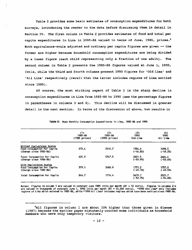
Table 2 provides some basic estimates of consumption expenditures for both
surveys, introducing the reader to the data before discussing them in detail in
Section IV. The first column in Table 2 provides estimates of food and total per
capita expenditures in Lima in 1985-86 valued in terms of June, 1985, prices.5
Both equivalence-scale adjusted and ordinary per capita figures are given -- the
former are higher because household consumption expenditures are being divided
by a lower figure (each child representing only a fraction of one adult). The
second column in Table 2 presents the 1985-86 figures valued at June 1, 1990,
Intis, while the third and fourth columns present 1990 figures for 'Old Lima' and
'All Lima, respectively (recall that the latter includes regions of Lima settled
since 1985).
Of course, the most striking aspect of Table 2 is the sharp decline in
consumption expenditures in Lima from 1985-86 to 1990 (see the percentage figures
in parentheses in columns 3 and 4). This decline will be discussed in greater
detail in the next section. In terms of the discussion of above, two results in
Table 2: Mean Monthly Consumption Expenditures in Lima, 1985-86 and 1990
(1) (2) (3) (4)1985-86 1985-86 1990 1990
(1985 prices) (1990 prices) Old Lima All Lima
Without Equivalence ScalesFood Consumption Per Capita 273.4 2510.7 1334.6 1298.5(Change since 1985-86) (-46.8%) (-48.3%)
TotaL Consumption Per Capita 625.9 5747.5 2821.5 2664.4(Change since 1986-86) (-50.9%) (-53.6%)
With Equivalence ScalesFood Consumption Per Capita 379.1 3480.9 1771.3 1757.0(Change since 1985-86) (-49.1%) (-49.5%)
Total Consumption Per Capita 846.7 7774.4 3679.7 3531.7(-52.7%) (-54.6%)
Notes: Figures in column 1 are vaLued in constant June 1985 Intis per month ($1 12 Intis). Figures in cotumns 2-4are valued in thousands of constant June 1, 1990 Intis per month ($1 = 50,000 Intis). "1990 Old Lima" onLy includesregions of Lima which existed in 1985-86, white "1990 ALl Lima" includes regions which have been settled since 1985-86.
5All figures in column 1 are about 10% higher than those given in Glewwe(1987) because the earlier paper mistakenly counted some individuals as householdmembers who were only temporary visitors.
- 13 -
Table 2 are worth noting. First, the use of household equivalence scales has
very little impact on the magnitude of the decline in consumption expenditures
relative to that resulting from the per capita (unadjusted by equivalence scales)
figures. This implies that the figures to be presented in this paper are
relatively insensitive to assumptions made concerning equivalence scales.
Second, although 'All Lima' is somewhat poorer than 'Old Lima', the difference
is very small relative to the overall decline in consumption expenditures that
has occurred since 1985-86.
At this point the preliminaries regarding the data have been completed.
Sections IV and V, which are the heart of this paper, will examine the data in
greater detail.
.
- 14 -

IV. Changes in the Distribution of Consumption from 1985-86 to 1990
This section examines both the 1985-86 and the 1990 expenditure data from
Lima, Peru, to see how Peruvians at different consumption levels fared during the
intervening 5 year period. The first subsection will examine changes in the
overall distribution of consumption expenditures by deciles. The second
subsection will examine changes in the different districts (areas) of Lima. The
third will examine the welfare of different social groups as defined by head of
household characteristics, and the fourth will discuss several other determinants
of household welfare resulting from the survey data.
Changes in the Overall Distribution of Consumption Expenditures
In order to examine changes in the distribution of consumption expenditures
from 1985-86 to 1990, the population of Lima was divided into ten expenditure
deciles for both surveys, where the first decile contains the poorest 10% of the
population as defined by equivalence scale adjusted per capita consumption
expenditures, the second contains the next poorest 10%, etc. and the tenth
contains the wealthiest 10%. Table 3 presents the mean levels of adjusted per
capita food and total consumption expenditures for each decile in both 1985-86
and 1990. The percentage decline in food and total per capita expenditures for
each group is given, as well as the fraction of total expenditures devoted to
purchases of food (in parentheses below the value of total expenditures). The
table compares Lima in 1985-86 with both 'All Lima' and 'Old Lima' in 1990, but
the main findings hold in both cases.
Several conclusions can be drawn from Table 3. The most striking is that
all groups experienced declines in the value of real food and total consumption
that left them at about one half of their 1985-86 levels, and for some groups the
decline was even sharper. The decline in average (equivalence scale adjusted)
per capita consumption for 'All Lima' was 55% (53% in 'Old Lima'), which
indicates a devastating fall in living standards in only 5 years. Another result
which is also striking is that the poorest decile seems to have lost the most,
- 15 -
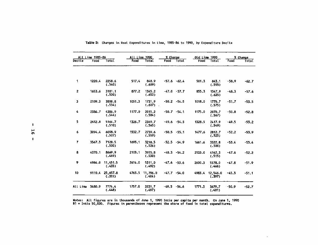
Table 3: Changes in Real Expenditures in Lima, 1985-86 to 1990, by Expenditure DeciLe
All Lima 1985-86 All Lima 1990 % Chanoe Old Lima 1990 % ChangeDecile Food TotaL Food Total Food Total Food Total Food Total
1 1220.4 2258.6 517.4 848.9 -57.6 -62.4 501.3 843.1 -58.9 -62.7(.540) (.609) (.595)
2 1653.6 3181.1 877.2 1345.2 -47.0 -57.7 855.3 1347.9 -48.3 -57.6(.520) (.652) (.635)
3 2109.3 3808.8 1051.3 1731.9 -50.2 -54.5 1018.0 1770.7 -51.7 -53.5(.554) (.607) - (.575)
4 2386.7 4386.9 1177.0 2015.2 -50.7 -54.1 1175.0 2070.7 -50.8 -52.8(.544) (.584) (.567)
5 2632.8 5164.7 1326.7 2349.7 -49.6 -54.5 1328.5 2417.9 -49.5 -53.2(.510) (.565) (.549)
cn 6 3094.4 6098.9 1532.7 2739.6 -50.5 -55.1 1477.6 2812.7 -52.2 -53.9(.507) (.559) (.525)
7 3567.3 7128.5 1693.1 3218.5 -52.5 -54.0 1661.6 3322.8 -53.4 -53.4(.500) (.526) (.500)
8 4070.1 8669.9 2103.1 3970.8 -48.3 -54.2 2133.0 4142.3 -47.6 -52.2(.469) (.530) (.515)
9 4984.0 11,451.5 2614.0 5311.0 -47.6 -53.6 2600.3 5578.0 -47.8 -51.9(.435) (.492) (.466)
10 9110.4 25,657.8 4763.5 11,796.0 -47.7 -54.0 4983.4 12,546.0 -45.3 -51.1(.355) (.404) (.397)
ALL Lima 3480.9 7774.4 1757.0 3531.7 -49.5 -54.6 1771.3 3679.7 -50.9 -52.7(.448) (.497) (.481)
Notes: All figures are in thousands of June 1, 1990 Intis per capita per month. On June 1, 1990S1 = Intis 50,000. Figures in parentheses represent the share of food in total expenditures.

having experienced declines of 58% and 62% of food and total consumption
respectively. Further, in terms of total consumption, the second poorest decile
experienced the next largest decline, a drop of 58%. Thus the evidence from
these two surveys indicates that the distribution of consumption expenditures
became more unequal during the Garcia years, despite the rhetoric put forth by
the Garcia administration that it was taking exceptional efforts to protect the
poor. This holds whether or not one looks at 'All Lima' or only 'Old Lima', and
whether one makes adjustments for equivalence scales or takes a simple per capita
estimate of total expenditures (see Appendix D for unadjusted figures). Recall
from Section III that although the possible bias in the data due to under-
reporting of expenditures by wealthy households cannot be detected, it may mean
that the average drop in consumption above is overestimated, while the regressive
change in the distribution of consumption expenditures may be underestimated.
The overall finding (Tables 2 and 3) that real expenditures declined
substantially from 1985-86 to 1990 might also be subject to question due to the
method used to calculate an appropriate price deflator for this period (see
Appendix B for details). However, in all deciles the share of total expenditures
devoted to food rises substantially. This suggests that living standards did
decline dramatically, since food shares tend to rise as families become poorer
and, of course, the measurement of food shares during the two survey periods does
not depend on the price deflator.
Finally, one may question whether these results are an artifact of over-
simplification in accounting for changes in both the level of prices and in
relative prices. To investigate this, a specific price index was calculated for
each household according to shares of food and non-food expenditures in total
household consumption. The results differ only slightly from those given here.
In particular, when consumption values are deflated using the new price indices
all deciles still experience drops in consumption expenditures to about one half
of 1985 levels, and the poorest decile experiences the largest decline. Details
of these calculations are given in Appendix E.
- 17 -

Changes in Consumption Expenditures by Areas within Lima
Table 4 presents means of both food and total expenditures, as well as the
food share, for 9 different areas of Lima for both 1985-86 and 1990. The
geographic demarcation of each area is given in Appendix F. For all areas of the
city the declines in average food and total expenditures were very large, but not
all regions suffered equally. The wealthiest area of Lima according to both food
and total expenditures was the 'Estrato Alto' ('Upper Class'). Households in
this area suffered the smallest declines in expenditures, and the share of food
in total expenditures for these households remained low relative to all other
areas and the city average. The second wealthiest area, 'Centro 3', experienced
slightly larger declines in both food and total expenditures.
The next three areas ranked in terms of 1985-86 total expenditures are
'Centro 1', 'Oeste' and 'Centro 2'. Of these three areas, 'Oeste' apparently
suffered the smallest declines, losing less than 50% of food and total
consumption per capita. 'Centro 1' was slightly better off than 'Centro 2' in
1985-86 in terms of average per capita total consumption. However, while both
areas experienced roughly the same decline in total consumption in percentage
terms, the decline in 'Centro 2' brought the absolute level of total consumption
in that area to levels approximating those in Callao in 1990, a notably poorer
area in 1985-86. Expenditures on food in these two areas fell by roughly fifty
percent, bringing food consumption in 'Centro 2' below the absolute level in
Callao and some of the apparently even poorer areas (in terms of total
expenditures). While this sharp drop in food expenditures may be due in part to
price differentials across areas, it is evident that a particularly rapid
cLeterioration in living standards has occurred in 'Centro 2' relative to other
aLreas.
The remaining four areas, 'Callao' and the Conos 'Norte', 'Sur', and 'Este'
(the Northern, Southern and Eastern Cones of the city), are those in which
significant geographic expansion has taken place since 1985-86 due to migration.
- 18 -

Table 4: Changes in Real Monthly Expenditures Per Capita, 1985-86 to 1990, by Area
Lima 1985-86 Lima 1990 % Chanre since 1985-86
Food FoodFood Total Share Food TotaL Share Food Total
SurOld regions 3,337.6 6,425.7 0.519 1,668.8 2,801.3 0.596 -50.0 -56.4ALL regions -- -- -- 1,699.3 2,785.6 0.610 -49.1 -56.6
NorteOld regions 3,002.1 6,430.9 0.467 1,453.0 2,788.9 0.521 -51.6 -56.6ALL regions -- -- -- 1,456.5 2,698.8 0.540 -51.5 -58.1
EsteOLd regions 3,110.8 7,625.7 0.428 1,441.8 2,576.6 0.560 -53.7 -64.5ALL regions -- -- -- 1,490.3 2,546.1 0.595 -52.1 -65.0
CallaoOld regions 3,211.0 6,849.0 0.469 1,744.8 3,760.8 0.464 -45.7 -45.1All regions -- -- -- 1,809.3 3,798.7 0.476 -43.6 -44.5
Oeste 3,342.2 7,804.9 0.428 2,001.8 4,425.8 0.452 -40.1 -43.3
Centro 1 3,461.7 8,177.5 0.423 1,723.3 4,054.3 0.427 -50.0 -50.4
Centro 2 3,474.6 7,491.0 0.464 1,577.2 3,726.8 0.422 -54.6 -50.2
Centro 3 4,335.0 11,550.4 0.377 3,003.4 6,501.6 0.462 -31.0 -43.7
Estrato Alto 5,388.0 16,934.5 0.318 3,832.7 9,960.7 0.385 -28.9 -43.0
LiSmaold regions 3,480.9 7,774.4 0.448 1,771.3 3,679.7 0.481 -49.1 -52.7All regions -- -- -- 1,757.0 3,531.7 0.497 -49.5 -54.6
Notes: All figures are in thousands of June 1, 1990 Intis per capita per month. On June 1, 1990S1 = Intis 50,000. Rows for "All regions" in 1985-86 are bLank because "ALL regions" includes regionswhich did not exit in 1985. See Text, Section 111.
As the survey sample was extended in 1990 to include these newly populated
regions, results are given in Table 4 for the 'Old' regions in each area which
were surveyed again in 1990, and for the area population as a whole ('All'
regions) in 1990. The most noticeable result is that while the incorporation of
the newly settled regions consistently lowers the area mean food and total
consumption values, it does so by very small and arguably statistically
insignificant amounts. This indicates that while average living standards in the
newly settled regions are low, they are not significantly worse than in each area
as a whole. The implication for targeting efforts is that the poorest members
of the population are not found in any great majority in the new settlements;
- 19 -

therefore, targeting programs specifically to these new settlements may not be
most efficient.
The largest percentage drops in total expenditures occurred in the Conos
Norte, Este and Sur. This finding is broadly consistent with that in the
previous section, which concluded that the poorest groups appear to have suffered
the most in the economic decline from 1985-86 to 1990. It should be noted that
the deterioration of living standards was most severe in the Cono Este. This
area, where expenditure levels were higher on average than in Callao and the
other Conos in 1985-86, had become the poorest in terms of total consumption by
1990. Callao seems to have fared slightly better than the three Conos,
experiencing a smaller percentage decline in both total and food expenditures.
Changes in consumption Expenditures by Head of Household Characteristics
Tables 5 and 6 examine changes in consumption expenditures from 1985-86 to
1990 when households are divided into groups based on the gender, education and
employment characteristics of the head of household. Table 5 shows the change
in mean total consumption per capita in Lima as whole between 1985-86 and 1990,
while Table 6 examines the change only in the 'Old' regions of Lima. The
figures, which represent mean total consumption, have again been adjusted for
each household's composition of children and adults. The percent of the total
population living in households where the head displays the given characteristic
is provided in the column to the right of total mean consumption in each year.
Table 6 has been provided to illustrate that when broken down by head of
household characteristics, households in 'old Lima' fared marginally but
consistently better than those in 'All Lima'. The following discussion will
refer to Table 5 unless a significant difference between the two tables requires
discussion.6
6Note also that, as in Table 3, the results shown in both Table 5 and 6remain essentially unchanged when price deflators based on each household'sconsumption patterns are used. For details see Appendix D.
- 20 -

Table 5: Changes in Per Capita MonthLy Expenditures by Characteristics of HousehoLd Head, ALL Lima
ALL Lima 1985-86 ALL Lima 1990 Percent Change inMean Expenditures (X of Pop) Mean Expenditures (% of Pop) Expenditures since 1985
SexMaLe 7,943.2 (86.6) 3,613.6 (85.4) -54.5FemaLe 6,681.0 (13.4) 3,012.2 (14.6) -54.9
Education LeveLNone 4,288.5 (2.8) 1,770.7 (3.5) -58.7Primary 5,677.6 (37.1) 2,324.4 (32.6) -59.1Secondary GeneraL 7,145.7 (35.4) 3,209.8 (44.1) -55.1Secondary TechnicaL 7,087.5 (5.3) 3,798.2 (2.3) -46.4University 15,112.2 (15.5) 6,945.7 (12.9) -54.0Other Post-Secondary 7,634.3 (3.9) 4,665.0 (4.6) -38.9
EmnLover of HeadGoverrment 9,474.3 (19.1) 4,155.0 (14.6) -56.1Private 7,604.0 (35.2) 3,321.2 (34.4) -56.3Private Home 3,931.5 (1.3) 1,782.4 (0.7) -54.7Setf-Employed 7,126.7 (36.3) 3,466.2 (36.4) -51.4
Occupation of HeadAgriculture 6,430.0 (3.7) 3,189.4 (2.1) -50.4SaLes/Services 7,532.4 (27.8) 3,259.3 (30.3) -56.7Industry/Crafts 5,858.5 (37.3) 2,793.3 (34.7) -52.3White Collar 11,307.8 (23.0) 5,195.3 (19.8) -54.1
UnempLoved 8,098.5 (2.9) 2,763.5 (5.1) -65.9
Retired 7,495.9 (4.9) 3,733.3 (6.9) -50.2
ALL Lima 7,774.4 100 3,531.7 100 -54.6
Notes: PopuLation percentages do not add to 100 due to missing information for 0.3% of observations in 1985-86and 1.8% in 1990. The mean expenditure level for those with Secondary TechnicaL training becomes 6252.4 forAll Lima, 1990, if one outlying value is incLuded in the calculations. This would represent a -11.8% changein expenditures since 1985.
Gender
It is first of all important to note that in 'All Lima' the position of
female-headed households relative to male-headed households changed very little
over the five year period in question. In both 1985-86 and 1990, mean
consumption levels for female-headed households were approximately 84% of those
of their male counterparts. The number of female-headed households increased
only slightly, from 13.4% to 14.6% of the population. This finding is exactly
the same for 'Old Lima'(Table 6), indicating that female-headed households are
distributed equally throughout the established and the newly settled regions of
the city. The general finding is that although female-headed households had
consistently lower consumption levels than those headed by males, they were
- 21 -

Table 6: Changes in Per Capita Monthly Expenditures by Characteristics of Household Head, Old Lima
ALL Lima 1985-86 Old Lima 1990 Percent Change inMean Expenditures (X of pop) Mean Expenditures (% of pop) Expenditures since 1985
SexMale 7,943.2 (86.6) 3,784.8 (85.4) -52.3Female 6,681.0 (13.4) 3,062.7 (14.6) -54.2
Education LevelNone 4,288.5 (2.8) 1,784.2 (3.3) -58.4Primary 5,677.6 (37.1) 2,324.0 (33.0) -59.1Secondary General 7,145.7 (35.4) 3,309.6 (41.0) -53.7Secondary Technical 7,087.5 (5.3) 3,836.7 (2.5) -45.9University 15,112.2 (15.5) 7,238.9 (15.0) -52.1Other Post-Secondary 7,634.3 (3.9) 4,775.3 (5.2) -37.4
Emtloyer of HeadGovernment 9,474.3 (19.1) 4,310.3 (15.9) -54.5Private 7,604.0 (35.2) 3,576.2 (30.3) -53.0Private Home 3,931.5 (1.3) 1,785.8 (0.7) -54.6SeLf-EmpLoyed 7,126.7 (36.3) 3,637.4 (36.7) -48.9
Occupation of HeadAgriculture 6,430.0 (3.7) 3,697.1 (1.5) -42.5SaLes/Services 7,532.4 (27.8) 3,349.7 (29.9) -55.5Industry/Crafts 5,858.5 (37.3) 2,874.2 (30.7) -50.9White ColLar 11,307.8 (23.0) 5,386.0 (22.3) -52.4
Unemploved 8,098.5 (2.9) 2,727.5 (5.4) -66.3
Retired 7,495.9 (4.9) 3,810.6 (8.9) -49.2
Notes: Population percentages do not add to 100 due to missing information for 0.3% of observations in 1985-86and 1.6% in 1990. The mean expenditure LeveL for those with Secondary Technical training becomes 6580.7 forALL Lima, 1990, if one outlying value is incLuded in the caLcuLations. This would represent a -7.1% change inexpenditures since 1985.
apparently able to maintain their relative economic position. Thus they were not
any more vulnerable to drops in living standards during the recent recession than
were their male-headed counterparts.
Education
Table 5 shows that in Lima, households headed by someone with no education
at all or with only primary education experienced the largest declines in
expenditures relative to those with higher levels of education. Expenditures for
households in these two categories fell by roughly equivalent amounts, 58.7% and
59.1%, respectively. Those with no education were significantly poorer than
those with primary education even in 1985-86, and in 1990 represented a small
(3.5%) but very poor category of households in Lima. More generally, households
- 22 -

in both of these categories exhibited mean expenditure levels well below other
categories even in 1985-86. The percentage declines in expenditures experienced
by these two groups were larger than for any other population group classified
by head of household characteristic (with the sole exception of the unemployed).
The education level attained by the head of household therefore appears to be a
significant indicator of poverty for the purposes of social program targeting in
Lima, both in terms of the household's relative position at any given time, and
in terms of its vulnerability to declines in living standards over time.
Households headed by someone with secondary general or university level
education fared only slightly better in terms of the percentage decline in
average consumption levels, but maintained absolute consumption levels higher
than any other educational category in both survey years. Households headed by
those with secondary technical (-46.4%) or other post secondary education levels
(-38.9%) exhibit falls in consumption which are significantly smaller in
comparison to other categories and to the city average (-54.6). Note that
households where the head has secondary technical training represent a small and
apparently declining population group (from 5.3% of the population in 1985-86 to
2.3% in 1990). The decline in expenditures experienced by households in this
category is the smallest compared to all other education categories except 'other
post-secondary', suggesting that technical education helps reduce vulnerability
to severe welfare loss. This finding is supported by an earlier study, based on
the 1985-86 survey data (Arriagada, 1989). The fact that those with higher
education and technical training also began the period with higher consumption
levels than average is consistent with the overall finding in Table 3 that the
distribution of expenditures became more unequal from 1985-86 to 1990.
Emiolovment
Classifying households according to the employer of the head casts more
light on what happened in Peru between 1985-86 and 1990. Households headed by
the self-employed, the largest category of households (34% in both years),
experienced a (moderately) smaller reduction in expenditure levels than average.
- 23 -

For these households, expenditures fell an average of 51.4% in 'All Lima' and
48.9% in 'Old Lima'. Further, the percentage of self-employed household heads
fell slightly in the bottom 2 quintiles and rose in the wealthier 2 quintiles.
However, in 1990 as in 1985-86, the fraction of households headed by the self-
employed was larger in the poorer quintiles than in the wealthier quintiles.
Households headed by those employed by the government or in the private
sector experienced larger declines than the self-employed, of 56.1 and 56.3% in
'All Lima' respectively. It is also significant to note that a very small
percentage of those in poorest quintile are government employees, both in 1985-86
(9.8%) and 1990 (9.4%). Finally, it should be noted that while households headed
by an individual employed in a private home are indistinguishable from the rest
in terms of the percentage drop in expenditures, these households began the
period with expenditures of roughly half of the population average. Households
in this category represent a very small and very poor segment of the total
population (0.7% in 1990).
Categorizing households by the economic sector in which the head is
eimployed (Occupation of Head, Table 5) adds very little to the analysis except
to reveal that those working in agriculture appear to have suffered slightly
simaller expenditure declines than average, especially in 'Old Lima' (Table 6).
In Lima, of course, this group represents a very small percentage of the
economically active population, which is also apparently declining (from 3.7% in
1985-86 to 2.1% in 1990 in 'All Lima'). The proportion of the population living
in households where the head is employed in the sales/services sector has
increased; however, this is also the category for whom expenditures have
deaclined the most (-56.7%) since 1985-86. Thus the only sector which appears to
have expanded in terms of economic activity is at the same time the one for which
average consumption levels have declined most precipitously (except for the
unemployed). It may be conjectured that this sector absorbed some of those heads
of households who lost or left jobs in other occupations.
Persons living in households where the head was or became unemployed
experienced by far the largest drop in consumption of any category (-65.9%), and
- 24 -

expanded from 2.9% to 5.1% of the population. Further, absolute expenditure
levels for these households were lower than for all employment categories except
for those employed in a private home. This situation is in sharp contrast with
the economic status of the unemployed in Lima in 1985-86, when households headed
by the unemployed had higher expenditure levels than all other occupational
categories except white collar employees.
Turning to tables 7, 8, and 9 further illuminates the change in economic
status of the unemployed. These tables present the distribution of the
population within expenditure quintiles broken down by these same head of
household characteristics. They point to a particularly significant change in
employment levels between 1985-86 and 1990. Whereas in 1985-86 heads of
household who were not working in any occupation were found in roughly equal
proportion across quintiles, by 1990 this was not at all the case. The
unemployment rate increased at a rapid pace in the lower quintiles, more than
tripling in the bottom quintile, and doubling in the second quintile.
Conversely, in the upper two quintiles the rate of unemployment was roughly the
same in the two survey years. This suggests that unemployment rose substantially
between 1985-86 and 1990, and that the bulk of these new unemployed are found
among the most poor. It may be conjectured that in 1985-86 the unemployed were
often those who were financially able to be selective as to their type of
employment, whereas by 1990 the body of unemployed was largely composed of those
in poorer deciles who simply could not find work.
To summarize, the best indicators of poverty in terms of characteristics
of the head of household appear to be level of education and type of employer.
Households headed by someone with no education and/or employed in private homes
were consuming 50% less per capita than the city average in 1990, which itself
had fallen by roughly half,since 1985-86. Those least vulnerable to declines in
consumption levels were those with secondary technical or post-secondary (non-
university) training. Those hardest hit by the recessionary conditions
prevailing after 1987 appear to have been the unemployed (more specifically,
those who become unemployed between 1985-86 and 1990), who were heavily
- 25 -

Table 7: Distribution of Population by Characteristics of HousehoLd Heads, by Quintile, All Lima, 1985-86
QuintiLe Quintile Adjusted Mean1 Quintite Quintite Quintile 5 Per Capita
(Poorest) 2 3 4 (WeaLthiest) Expenditures
SeK of HeadMaLe 84.2 85.3 85.7 86.6 91.3 7,943.2FesaLe 15.8 14.7 14.3 13.4 8.7 6,681.0
Education of HeadNone 5.4 5.0 2.0 1.2 0.5 4,288.5Primary 58.3 43.9 40.6 27.5 15.3 5,677.6Secondary GeneraL 28.0 38.0 38.9 41.1 30.9 7,145.7Secondary Technical 1.8 6.2 4.5 9.7 4.1 7,087.5University 3.4 4.1 10.1 15.5 44.5 15,112.2Other Post-Secondary 6.5 2.8 3.9 5.1 4.7 7,634.3
EmpLoyer of HeadGoverrment 9.8 12.6 18.3 24.9 29.8 9,474.3Private 41.6 35.3 34.2 32.3 32.5 7,604.0Private Home 3.7 1.2 0.8 0.5 0.0 3,931.5SeLf-EmpLoyed 40.0 43.5 36.7 32.4 29.0 7,126.7
Occupation of HeadAgriculture 2.3 4.7 5.9 3.7 1.8 6,430.0Sales/Services 34.6 27.3 24.2 23.4 29.2 7,532.4Industry/Craft 47.6 49.9 38.6 35.3 15.1 5,858.5White Collar 10.6 10.6 21.2 27.3 45.1 11,307.8
Unemployed 2.1 3.2 3.0 2.8 3.6 8,098.5
Retired 2.5 4.3 6.2 7.2 4.6 7,495.9
Notes: CoLumns may not add to 100 due to missing information for 1.6% of observations. Figures represent thepercentage of the popuLation within each auintile in househoLds where the head dispLays the givencharacteristic.
represented in the poorest two quintiles in 1990 and whose consumption per capita
fell by 65.9% on average. Note however that even in 1990, households headed by
the unemployed represented a small percentage of the population in the poorest
quintile (7.8%). This suggests that while addressing unemployment will benefit
some of the poor, other complementary programs are required to reach the numerous
poor households not headed by the unemployed.
Other Indicators of Living Standards
This subsection discusses the change in living standards observed in Lima
between 1985-86 and 1990 based on housing conditions and ownership of durable
goods across quintiles and geographical areas of the city. The indicators for
housing point graphically to a widespread deterioration in physical living
- 26 -

Table 8: Distribution of Population by Characteristics of Household Heads, by Quintile, All Lima, 1990
Quintile Quintile Adjusted Mean1 Quintile Quintite QuintiLe 5 Per Capita Percent Change
(Poorest) 2 3 4 (WeaLthiest) Expenditure from 1985-86
Sex of HeadMaLe 83.6 84.0 83.3 90.1 87.6 3,613.6 -54.5Female 16.4 16.0 16.7 9.9 12.4 3,012.2 -54.9
Education of HeadNone 7.9 4.8 2.8 0.7 0.9 1,770.7 -58.7Primary 55.9 39.8 31.2 24.8 12.2 2,324.4 -59.1Secondary General 32.5 41.2 51.4 49.9 38.8 3,209.8 -55.1Secondary TechnicaL 2.1 2.0 3.1 2.2 2.5 6,252.4 -11.8University 1.1 7.7 8.8 14.1 37.1 6,945.7 -54.0Other Post-Secondary 0.5 4.5 2.7 8.4 8.5 4,665.0 -38.9
EmaLover of HeadGoverment 9.4 11.5 13.7 18.9 22.4 4,155.0 -56.1Private 35.3 28.3 34.6 35.6 29.6 3,321.2 -56.3Private Home 1.6 0.9 1.2 0.1 0.0 1,782.4 -54.7Self-Employed 39.4 40.7 35.5 33.5 33.4 3,466.2 -51.4
Occupation of HeadAgricuLture 2.2 2.8 0.2 1.5 2.8 3,189.4 -50.4Sales/Services 36.2 26.4 32.5 29.1 26.5 3,259.3 -56.7Industry/Craft 44.2 36.5 35.0 32.2 17.1 2,793.3 -52.3White Collar 4.3 16.5 17.7 26.0 39.6 5,195.3 -54.1
UnempLoyed 7.8 7.8 4.9 2.6 3.1 2,763.5 -65.9
Retired 4.9 9.6 7.7 7.8 8.9 3,733.3 -50.7
Notes: CoLumnfs may not add to 100% due to missing information for 1.8% of observations. Figuresrepresent the percentage of the population within each quintile in househoLds where the head displaysthe given characteristic.
conditions in metropolitan Lima between 1985-86 and 1990, which was most severe
in the Conos Sur, Este and Norte. Patterns in durable good ownership reflect
fairly similar levels of access to basic goods across all quintiles, but to
increasingly skewed ownership of luxury goods such as color televisions and cars.
Because these findings do not depend directly on price data, they are independent
of the deflators used in this paper. They therefore serve to confirm that living
standards declined substantially between 1985-86 and 1990, and that the sharpest
decline occurred among the poorest population quintiles.
Housing Conditions
Tables 10 and 11 in this section compare housing conditions in Lima in
1985-86 with 'All Lima' 1990 broken down by quintile, and top and bottom decile.
- 27 -

Table 9: Characteristics of Household Heads by Quintile, Old Lima, 1990
Quintile Quintile Adjusted Mean1 Quintile Quintile Quintile 5 Per Capita Percent Change
(Poorest) 2 3 4 (Wealthiest) Expenditures from 1985-86
Sex of HeadMate 83.9 84.2 81.2 91.3 86.6 3,784.8 -52.3Female 16.1 15.3 18.8 8.7 13.4 3,062.7 -54.2
Education of HeadNone 6.5 6.1 3.3 0.0 1.1 1,784.2 -58.4Primary 54.5 40.3 33.2 26.1 9.7 2,324.0 -59.1Secondary General 34.4 37.6 47.4 47.7 36.8 3,309.6 -53.7Secondary Technical 3.2 2.2 3.8 1.7 3.6 6,580.7 -7.1University 1.3 9.4 8.5 15.3 40.4 7,238.9 -52.1Other Post Secondary 0.0 4.4 3.8 9.1 8.3 4,775.3 -37.9
EmoLoyer of HeadGovernment 9.1 12.5 14.1 20.1 22.7 4,310.3 -54.5Private 35.6 23.3 32.0 33.3 27.4 3,576.2 -53.0Private Home 1.7 0.9 1.4 0.0 0.0 1,785.8 -54.6SeLf-EmpLoyed 40.0 41.6 35.7 32.6 34.1 3,637.4 -49.0
Occupation of HeadAgriculture 2.0 1.2 0.0 1.2 3.0 3,697.1 -42.5Sales/Services 37.7 26.1 33.0 27.4 25.6 3,349.7 -55.3Industry/Craft 43.8 33.9 32.7 29.0 15.8 2,874.2 -50.9White Collar 4.1 17.5 18.0 29.2 40.5 5,386.0 -52.4
Unemployed 7.5 8.6 5.1 3.0 3.3 2,727.5 -66.3
Retired 4.9 12.0 8.8 9.1 9.9 3,810.6 -49.2
Notes: CoLumns may not add to 100% due to missing information for 2.0% of observations. Figuresrepresent the percentage of the population within each quintile in households where the head displays the givencharacteristic.
A further category, top and bottom 5 percent, has been added to the tables for
1990. The inclusion of this category highlights distinct characteristics of the
poorest segment of the population of Lima, and makes clear the particularly
skewed nature of living conditions in the city by emphasizing the markedly better
living conditions of the population in the top 5 percent of expenditure levels.
Tables 12 and 13 display the same characteristics for the population broken down
by geographic area. These tables point to strong regional differences and to the
rapid deterioration in physical living conditions between 1985-86 and 1990.
Comparing Tables 10 and 11, it is evident that home ownership pertains
rather equally to all expenditure groups in both 1985-86 and 1990. This
characteristic is therefore not 'highly significant in locating the poorest
households, particularly since after 1985 land titles were [ssued sporadically
- 28 -
Table 10: Distribution of Population by Housing Characteristics, ALL Lima 1985-86, by Quintile
QuintiLe Quintile1 Quintile Quintile Quintile 5 All
Bottom 10% ALL 2 3 4 ALL Top 10% Lima
Type of HomeSingle famiLy BuiLding 64.6 66.5 63.7 57.8 62.7 63.4 65.3 62.7Multi-famiLy BuiLding 12.5 11.8 15.6 14.5 11.6 6.8 3.5 11.6Apartment 5.2 6.4 9.4 12.8 15.6 22.8 26.5 14.4Quinta 9.4 7.9 7.1 11.6 7.6 5.5 4.1 7.8Shack 8.3 6.9 4.2 3.2 2.5 1.5 0.6 3.5
How occupiedowned 62.0 61.3 57.0 50.4 53.6 56.0 58.9 55.3Rented 20.0 22.2 24.8 29.9 29.9 31.7 31.4 28.3Invasion 9.0 6.1 2.2 4.0 3.1 0.9 0.6 3.0Other 9.0 10.4 16.1 15.7 L3.4 11.4 9.1 13.3
Material of WallsBrick, Cement 72.0 72.6 68.7 75.5 83.5 88.0 92.0 78.8Adobe 12.0 12.7 18.3 11.3 11.0 7.3 6.3 11.6Wood 8.0 5.2 3.0 3.6 0.0 1.5 0.6 2.4Straw Mat 4.0 5.2 4.8 4.4 3.8 1.8 0.6 3.8Sugar Cane 1.0 1.9 3.9 1.5 1.0 1.2 0.6 1.8Stone, Mud, Other 3.0 2.4 1.3 3.6 0.7 0.3 0.0 1.6
Source of WaterIn Home 67.0 68.9 68.3 74.4 76.6 88.6 93.7 76.6Truck 7.0 8.0 6.1 4.0 5.8 1.8 0.6 4.8Public Standpipe 3.0 3.8 5.2 3.6 4.5 1.2 0.6 3.5In Building 17.0 14.1 13.0 13.5 11.0 6.2 3.4 11.1WelL/Canal 3.0 3.3 3.5 1.8 0.7 2.0 1.7 2.1
Have Sewage SYstem 88.0 90.6 91.3 93.4 94.5 98.8 100.0 94.2
Source of LightElectricity 90.0 92.0 96.1 94.5 94.8 98.2 100.0 95.4Gas/Kerosene 7.0 6.1 3.0 3.6 2.7 0.6 0.0 3.0Candle 3.0 1.9 0.9 1.8 2.1 1.2 0.0 1.6
Cooking Fuel UsedElectricity 0.0 0.5 1.3 1.5 3.1 15.2 21.7 5.1Gas 14.0 13.7 16.1 31.0 41.2 59.5 62.9 35.2Kerosene 84.0 84.9 80.9 66.1 52.6 24.0 15.4 58.0Coal/Wood 0.0 0.0 0.4 0.0 0.0 0.0 0.0 0.1
Notes: Figures represent the percentage of population within each cuintile in households displayingthe given characteristic. Columns may not add to exactly 100% due to rounding, and to responses whichhave not been listed due to insignificant percentage values. Ownership by "Invasion" indicates thatoccupants do not possession a title of land ownership.
by the government (for political purposes) in some regions of the Conos Norte,
Este and Sur which had been recently settled by invasion. Correspondingly, the
incidence of occupation by invasion apparently increased dramatically between
1985-86 and 1990, especially in the bottom 2 quintiles. It is therefore likely
that many who reported ownership as defined by the questionnaire (possessing a
land title) had in fact invaded the land. Renting a home declined across all
- 29 -

Table 11: Housing Characteristics, ALL Lima, 1990, by Expenditure Quintile
QuintiLe QuintiLe1 5
Bottom Bottom QuintiLe Quintile Quintile Top Top ALL5% 10% ALL 2 3 4 ALL 10% 5% Lima
Type of HomSingle famiLy Building 76.1 77.6 75.8 70.8 71.0 71.5 75.2 73.4 73.5 72.9MuLti-family BuiLding 6.6 6.2 7.4 8.0 9.0 4.8 2.0 1.7 2.2 6.2Apartment 3.1 2.0 3.9 6.1 6.3 9.8 15.0 19.5 20.5 8.2Quinta 2.8 2.2 1.6 4.8 7.2 7.5 4.9 3.6 3.5 5.2Shack 11.4 12.0 11.5 10.3 6.5 6.4 2.8 1.7 0.3 6.9
How OccupiedOwned 53.7 58.6 52.7 52.9 59.3 57.4 62.9 63.8 67.8 56.0Rented 10.9 7.9 10.5 16.9 17.4 17.5 21.8 22.0 22.7 16.8Invasion 26.6 24.4 23.4 23.1 16.6 15.2 9.1 7.4 1.9 17.5Other 8.7 9.1 12.3 7.2 6.6 9.8 6.1 6.8 7.6 9.4
Material of WaLLsBrick, Cement 67.0 66.2 69.8 72.3 77.0 78.9 90.0 93.1 95.1 77.6Adobe 8.4 6.0 6.8 8.1 9.2 10.7 4.1 2.8 2.4 7.8Wood 6.1 6.3 6.0 5.7 3.9 2.8 1.8 1.3 0.0 4.0Straw Mat 15.3 18.2 14.3 10.6 6.5 5.6 2.4 1.4 0.1 7.9Sugar Cane 0.0 0.8 1.3 2.5 3.0 1.8 1.1 1.1 2.2 1.9Stone, Mud, Other 3.1 2.5 1.8 3.2 3.4 1.9 1.7 0.2 0.2 0.8
Average Number ofRooms per Person 0.3 0.4 0.5 0.5 0.8 0.9 1.4 1.7 2.0 0.9Source of WaterIn Home 52.0 57.3 52.8 61.8 75.2 74.4 85.9 91.3 98.6 70.0Truck 21.1 20.0 17.1 14.1 10.3 9.2 7.9 4.4 0.3 11.7Public Standpipe 19.5 15.2 16.7 10.3 6.1 7.3 2.4 0.9 0.8 8.6In Building 6.9 4.9 8.l 6.3 5.5 8.0 2.6 2.0 0.0 6.1Well/Canal 0.5 2.5 4.9 6.4 1.9 0.9 1.1 1.3 0.3 3.0
Hours of Public WaterService Per DaYNone 21.6 22.4 22.3 21.5 13.2 10.3 9.1 6.4 0.6 15.51-3 29.2 23.5 24.5 17.3 19.7 15.6 15.5 11.3 11.4 18.54-6 15.6 13.3 16.9 17.3 23.0 27.2 20.7 22.0 28.1 21.07-12 14.2 21.7 18.4 24.5 25.7 29.9 33.1 36.8 44.3 26.313 or more 19.4 19.0 17.8 18.9 18.5 16.6 21.3 23.5 15.6 18.6
Have Sewage System 60.1 63.5 57.0 62.9 71.8 77.1 88.5 93.2 97.9 71.5
Source of LightELectricity 85.2 87.1 84.6 86.0 92.6 92.7 96.9 98.6 99.5 90.5Gas/Kerosene 12.8 9.7 10.6 10.8 6.1 5.1 2.7 1.3 0.5 7.1Candle 0.9 2.7 4.0 3.2 1.0 1.9 0.3 0.1 0.0 2.1
Cooking Fuel UsedELectricity 0.0 0.0 0.0 0.0 0.5 2.6 8.8 15.0 24.0 2.4Gas 8.7 11.7 12.0 31.8 43.0 51.4 67.7 72.2 69.7 41.2Kerosene 90.6 87.8 87.1 67.5 55.8 45.1 23.3 12.8 6.3 55.7CoaL/Wood 0.6 0.3 0.8 0.5 0.0 0.0 0.0 0.0 0.0 0.3
See notes, Table 10.
- 30 -

quintiles, but by unequal proportions: renting by 1990 became a distinct
characteristic of the wealthier expenditure groups.
The quality of homes deteriorated significantly for households in the
bottom expenditure quintile (representing the poorest 20% of the population),
where the incidence of housing made of "estera" (straw mats) approximately
trebled between 1985-86 and 1990. Turning to public services, the number of
households with water service in-home decreased consistently in the lower
quintiles between 1985-86 and 1990. The glaringly uneven distribution of public
services is also evident. In 1990 a full 98.6% of households with expenditures
in the top 5% of the distribution had public water service in their homes, while
this service was available to roughly half of those in the bottom 5% of the
distribution. The situation is similar for access to public sewage systems;
97.9% of those in the highest expenditure category had a sewage system in their
homes, while only 60.1% of those in the lowest category had this service.
For 1990 an additional category of information is available, detailing the
average hours of water service available to those served by the public system.
This question was added because after 1985-86 public water services deteriorated,
so that by 1990 some areas were receiving little or no water at all from public
pipes. From the results it is clear that in 1990 the lower expenditure groups
were receiving the least water from public services, with 21% in the poorest
quintile receiving no water at all.
There is one further characteristic of the lower quintiles which is
noteworthy. A vast proportion of households at these lower expenditure levels
depend on kerosene for cooking fuel--in 1990, 90.6% of households in the bottom
5% of the distribution in terms of household expenditures were cooking with
kerosene. Furthermore, it is clear from Table 11 that the usage of kerosene
increases distinctly as expenditure levels drop. This is a significant factor
to recall when considering the taxation or subsidization of kerosene, which will
be discussed further in Section V.
Tables 12 and 13 present these same housing characteristics as distributed
within the 9 geographical areas of Lima. They confirm the findings resulting
- 31 -

from Tables 10 and 11, highlighting in particular the geographical areas where
public services deteriorated most significantly between 1985-86 and 1990. In the
Cono 'Este', the area with the lowest per capita expenditure levels in 1990
(Table 4), the provision of public services was also consistently the poorest in
1990 (although levels in the Cono Sur and Norte were only slightly better): 33%
of households in the Cono 'Este' were not served by public water pipes, 20% had
no electricity, and 48% had no sewage system. On the other hand, the
deterioration since 1985-86 in the level of public services provided appears to
have been most acute in the Cono 'Norte', where in 1985-86 the percentage of
households with water in-home, with access to a sewage system and with
electricity was slightly higher than in the other two Conos. This was no longer
the case in 1990, where the Cono 'Sur' surpassed the Cono 'Norte' in the
provision of both water in-home and electricity.
Durable Good Ownership
one convenient and intuitively appealing dimension of living standards is
household ownership of various durable goods. Tables 14 and 15 provide this
information for both 1985-86 and 1990, by quintile and by area of Lima
respectively. The durable goods considered are radios, refrigerators, cars,
bicycles, color and black-and-white televisions and gas stoves.
For Lima as a whole, ownership of the above mentioned durable goods was
quite stable. The sole exception is the ownership of radios, which has increased
substantially for all expenditure groups. Refrigerator and car ownership
declined slightly in all quintiles, but changes in the ownership of other goods
vary somewhat by quintile.
The extent to which durable goods are found primarily in households at
certain income levels can be useful for purposes of identifying the poor.
Generally speaking, in Lima radios and black and white televisions are found in
the same proportion among the different quintiles. By contrast, the other five
durable goods are more likely to be found among the better off households. The
most stark contrasts are apparent in the ownership of cars, color televisions and
- 32 -

Table 12: Distribution of Population by Housing Characteristics, ALl Lima, 1985-86, by Area
Sur Norte Este Oeste CaLLao Centro 1 Centro 2 Centro 3 Estrato Alto
Tyoe of HomeSingle Family Building 86.3 84.4 86.4 36.8 86.3 35.4 31.1 52.9 39.4Multi-Family Building 3.0 6.2 5.2 18.9 13.0 6.2 21.0 20.7 10.6Apartment 0.0 3.3 3.1 18.9 9.2 22.9 31.5 18.4 43.9Quinta 0.6 0.5 1.6 24.5 1.5 35.4 14.8 8.0 6.1Shack/Other 10.1 5.7 3.1 0.9 2.3 0.0 1.6 0.0 0.0
How occupiedOwned 68.9 59.9 68.8 36.6 62.0 41.7 31.6 55.5 62.1Rented 6.7 11.2 16.4 53.6 26.3 41.7 53.2 36.7 28.8Invasion 8.3 2.6 1.9 0.0 0.7 2.1 4.9 0.0 0.0Other 16.1 21.1 13.0 9.8 10.9 14.6 10.3 7.8 9.1
Material of WallsBrick, cement 73.6 86.6 87.9 66.1 84.7 66.7 74.9 68.9 84.8Adobe 0.5 2.6 8.7 31.2 2.9 33.3 16.0 28.9 13.6Wood 4.7 5.2 0.5 0.9 1.5 0.0 2.3 2.2 0.0Straw Mat 16.6 3.4 2.9 0.0 1.5 0.0 1.1 0.0 0.0Sugar Cane 0.5 0.0 0.0 1.8 8.8 0.0 3.0 0.0 1.5
w Stone, Mud, Other 4.1 2.1 0.0 0.0 0.7 0.0 2.7 0.0 0.0
Source of WaterIn Home 72.0 72.4 68.1 79.5 81.7 97.9 76.8 81.1 72.0Truck 10.9 13.4 5.3 0.0 1.5 0.0 0.0 0.0 10.9Public Standpipe 2.6 0.9 10.1 0.0 3.6 0.0 5.3 0.0 2.6In BuiLding 9.3 7.8 5.3 18.7 12.4 2.1 16.0 18.9 9.3Well/Canal 1.0 2.6 9.6 0.0 0.0 0.0 0.4 0.0 1.0
Have Sewage System 83.9 97.4 89.9 96.4 96.3 100.0 97.3 96.7 98.5
Source of LishtElectricity 93.8 95.7 90.3 97.3 97.8 100.0 96.6 96.7 97.0Gas/Kerosene 4.1 3.0 4.3 2.7 0.7 0.0 3.0 2.2 3.0Candle 2.1 1.3 4.8 0.0 1.5 0.0 0.4 1.1 0.0
Cooking Fuel UsedElectricity 0.0 0.4 4.8 1.8 2.9 10.4 5.7 12.2 31.8Gas 16.6 30.6 25.1 56.2 46.0 52.1 36.9 40.0 53.0Kerosene 82.4 67.7 67.6 40.2 50.4 33.3 55.1 45.6 15.1Coal/Wood 0.0 0.0 0.5 0.0 0.0 0.0 0.0 0.0 0.0
Note: Figures represent the percent of the population within each area living in households displaying the given characteristic.

Table 13: Distribution of Population by Housing Characteristics, ALL Lima, 1990, by Area
Sur Norte Este Oeste CalLao Centro 1 Centro 2 Centro 3 Estrato Alto
Type of HomeSingLe FamiLy Building 80.1 91.5 83.6 42.9 75.7 34.4 48.9 59.1 49.6Multi-Family Building 3.0 1.2 1.4 12.2 8.3 1.8 15.9 21.9 7.0Apartment 0.8 0.5 1.2 11.7 8.6 23.9 26.6 9.7 36.0Quinta 0.4 1.2 0.3 30.0 1.4 37.4 8.4 8.2 7.5Shack/Other 15.6 5.6 13.8 3.2 6.0 2.4 0.1 1.1 0.0
How OccupiedOwned 51.5 55.3 63.9 52.1 74.8 61.3 44.8 59.5 57.5Rented 3.6 6.1 8.1 46.4 17.5 38.6 33.9 32.3 37.3Invasion 37.5 28.3 18.4 0.0 1.3 0.0 6.9 1.8 2.6Other 7.4 10.3 9.6 1.5 6.4 0.0 13.4 6.4 2.6
Material of WallsBrick, cement 75.9 78.1 78.8 76.2 76.7 82.2 78.2 69.2 86.4Adobe 0.9 6.7 3.1 21.6 1.9 11.0 15.5 29.0 7.0Wood 4.9 6.4 3.4 0.0 5.6 0.0 2.5 1.8 2.6Straw Mat 16.7 7.7 13.5 0.0 6.0 0.0 0.5 0.0 0.0Sugar Cane 0.0 0.5 0.2 2.2 9.0 4.3 3.2 0.0 3.9Stone, Mud, Other 1.5 0.6 1.1 0.0 0.8 2.4 0.0 0.0 0.0
Average Number ofRooms per Person 0.7 0.8 0.7 1.2 0.8 1.4 0.9 1.3 1.6Source of Water
v In Home 64.0 61.3 58.1 89.8 80.3 97.5 79.3 79.6 81.6Truck 18.0 14.2 27.9 0.0 2.2 0.0 0.0 0.0 0.0PubLic Standpipe 8.6 18.3 5.6 5.0 8.3 0.0 5.4 0.0 0.0In Building 1.3 2.8 2.4 5.2 7.8 2.4 14.2 20.4 18.4Well/Canal 6.8 2.6 5.3 0.0 0.9 0.0 1.1 0.0 0.0
Hours of Public Water ServicePer daYNone 26.5 17.7 33.9 1.5 3.6 0.0 1.1 0.0 0.01-3 32.9 19.9 17.2 9.9 7.3 8.0 19.8 10.0 8.34-6 12.6 20.4 14.5 25.6 33.4 39.9 29.5 15.4 14.97-12 7.1 25.0 22.1 45.7 41.2 39.3 28.3 27.2 53.113 or more 20.9 17.0 12.3 17.4 14.6 12.9 21.3 47.3 23.7
Have Sewage System 61.7 65.0 57.9 87.8 80.8 100.0 83.7 86.4 84.6Source of LightElectricity 93.4 84.6 80.9 100.0 93.9 100.0 95.3 100.0 100.0Gas/Kerosene 4.8 11.2 13.7 0.0 5.7 0.0 3.9 0.0 0.0Candle 1.7 3.5 4.6 0.0 0.4 0.0 0.8 0.0 0.0
Cooking Fuel UsedElectricity 0.4 0.0 0.7 3.0 0.0 10.4 3.0 3.2 32.9Gas 27.0 33.3 31.9 70.5 58.6 62.0 44.7 58.8 52.6Kerosene 72.4 65.2 66.7 26.5 41.4 25.8 51.8 36.2 14.5Coal/Wood 0.1 1.0 0.2 0.0 0.0 0.0 0.0 0.0 0.0
Note: Figures represent the percent of the population within each area Living in househoLds displaying the given characteristic.

gas stoves. In 1990, only 2% of the population in the poorest quintile lived in
households with cars, compared to 37% for the wealthiest quintile. The analogous
figures for color televisions are 5% and 67%, and for gas stoves they are 16% and
74%. Further, no household in the poorest 5% of the population owed either a car
or a color television in 1990.
One fact which is not reflected in Tables 14 and 15 is that the vast
majority of durables (90%) were acquired before or during 1988, which implies
that when the economic decline began in late 1988 households coped by delaying
purchases of durable goods. This and other strategies of dealing with large
drops in household incomes will be examined in a separate paper; Section V will
examine patterns in durable good ownership for the purposes of targeting social
programs.
- 35 -

Table 14: Change in Distribution of Durable Good ownership, 1985-86 to 1990, 'ALL Lima,' by Quintile
QuintiLe QuintiLe1 Quintite Quintile Quintite 5
Durable Goods Year Bottom 5% Bottom 10% ALL 2 3 4 ALL Top 10% Top 5%
Radio 1990 82.5 81.2 80.3 83.2 84.4 88.9 90.6 91.0 95.31985 67.0 65.0 65.6 61.2 61.7 57.8 64.7 68.6 67.8
Refrigerator 1990 46.6 42.6 43.1 50.1 65.3 71.1 84.6 91.1 94.91 1985 30.4 43.0 48.2 56.1 67.4 75.5 87.4 93.5 97.0
w Car 1990 0.0 0.0 2.1 4.3 6.9 20.6 36.9 46.8 62.11985 0.0 1.9 3.4 5.0 7.9 18.8 45.1 55.6 67.0
Bike 1990 4.4 6.7 6.8 19.1 23.3 31.8 40.8 45.3 53.61985 9.3 7.0 10.2 18.2 16.2 26.1 35.5 36.6 31.6
Color TV 1990 0.0 4.0 5.0 19.2 34.0 46.6 67.3 81.3 93.21985 1.7 6.6 9.0 15.1 27.5 40.3 68.6 75.4 82.9
Black & white TV 1990 68.4 67.6 73.9 72.8 73.6 72.4 66.8 61.5 57.91985 68.1 73.5 73.7 80.5 70.8 74.5 67.9 62.5 61.4
Gas stove 1990 17.2 15.4 16.3 41.8 52.7 62.5 73.9 78.0 78.51985 20.9 23.4 26.6 35.1 48.2 62.9 70.2 70.6 64.6

Table 15: Change in Distribution of DurabLe Good Ownership, 1985-86 to 1990, All Lima, by Area
Durable Goods Year Sur Norte Este Oeste Callao Centro 1 Centro 2 Centro 3 Estrato ALto
Radio 1990 84.6 86.5 80.6 84.9 86.9 87.7 86.2 94.3 91.21985 60.5 57.5 66.9 67.6 62.1 70.4 58.3 63.7 70.0
Refrigerator 1990 53.0 57.7 53.4 81.9 68.1 86.5 67.1 75.6 92.11985 54.5 66.0 62.7 77.2 68.1 90.0 67.2 75.8 84.8
Car 1990 9.9 7.2 10.4 28.0 14.8 20.2 11.0 34.0 54.41985 8.3 10.0 8.4 25.0 18.2 25.4 18.7 25.1 53.6
Bike 1990 17.3 22.1 19.4 34.7 24.3 44.8 26.1 34.0 47.41985 14.3 19.8 22.9 23.2 28.8 31.4 14.1 31.5 33.8
BLack & white TV 1990 73.5 74.9 65.2 77.2 80.3 65.0 70.8 68.1 59.61985 74.1 73.0 78.1 73.6 73.8 67.3 73.2 70.1 63.5
CoLor TV 1990 17.3 24.3 24.8 67.7 36.6 63.8 44.5 50.5 83.81985 19.7 23.0 27.1 49.2 32.3 51.8 32.8 48.8 70.0
Gas stove 1990 35.0 44.4 35.9 78.7 71.8 69.3 52.5 58.1 66.71985 33.2 49.8 41.5 66.4 59.7 63.6 50.0 50.7 52.8

V. Poverty in Lima from 1985-86 to 1990
The previous section examined changes in the overall distribution of
consumption in Lima between 1985-86 and 1990. This section focuses on those
households whose consumption is so low that they can be categorized as poor.
Subsection A discusses how the increase in poverty since 1985-86 may be
quantified using several definitions of an absolute poverty line. Subsection B
examines some distinct characteristics of the poor, focusing on how extremely
poor groups may be identified for targeting purposes.
Measuring the Incidence of Poverty in Lima
There is no official or widely accepted poverty line in Lima. This
subsection will examine several different methods of deriving such a line. To
keep the analysis simple, a standard head-count definition of aggregate poverty
will be applied. In other words, poverty will be measured in terms of the
fraction of the total population that are classified as poor. Households are
classified as poor if their per capita consumption levels, adjusted for household
composition as explained in Section III, fall below the particular poverty line
in question. The reader should bear in mind that any definition of poverty
necessarily involves certain value judgments regarding the adequacy of a
particular consumption level. However, it will be evident from the discussion
below that the increase in poverty in Lima was very large between 1985-86 and
1990 over a fairly wide range of possible definitions of poverty.
Table 16 presents figures on the extent of poverty in Lima in both years,
using six different definitions of the poverty line. The first two poverty lines
are based on the cost of a minimum basket of food for a family of six in Lima7.
The daily cost of this basket per family in June 1, 1990 Intis is 154,416, which
implies a cost of 4,632,480 Intis per month. The family is assumed to consist
of two adults and four children. Adjusting the resulting per capita value of the
7Source: Cuanto S.A., Lima, Peru. This food basket (Canasta Basica)provides 2,168.8 Kcal and 62.3 grams of protein per capita per day.
- 38 -

Table 16: Poverty Lines Based on Monthly Real Expenditures
Value of Poverty Line, Percent of PoouLation BeLow PovertY Line in:Poverty Line June 1, 1990 Intis ALL Lima 1985-86 ALL Lima 1990 OLd Lima 1990 New Lima 1990
1. Food Expenditures 1,447,650 12.7 54.7 55.8 49.3per capita below'Basic Needs' Food Basket
2. Total Expenditures 1,447,650 0.5 17.3 17.2 17.9per capita below'Basic Needs' Food Basket
3. TotaL Expenditures below 1,033,000 0.03 7.8 7.8 7.41985 Minimum Wage
4. TotaL Expenditures below 2,066,000 2.7 36.9 35.2 46.01985 Minimum Wage x 2
5. Total Expenditures below 695,900 0.0 2.6 2.6 2.41990 Minimun Uage
6. TotaL Expenditures below 1,391,800 0.5 15.7 15.8 15.61990 Minimum Waae x 2

food basket for household composition as in Section III, we assume that two of
the children are age 6 or younger, the third is 7-12 years old and the fourth is
13-17 years old. Thus the number of adult equivalents in the family is 3.2 [2(1)
+ 2(0.2) + 0.3 + 0.5]. This implies a poverty line of 1,477,650 Intis per adult
equivalent. Taking into account each household's composition of adults and
children, if one categorizes as poor any household for whom per capita total
consumption is less than this figure (so that even if all the household's money
was spent on food it could not purchase the minimum amount of food required for
each of its members) only 0.5% of the population of Lima was poor in 1985-86.
However, if one categorizes as poor the households where per capita food
expenditures are less than this amount, 12.7% of Lima's population was poor in
1985-86.
The other four poverty lines are defined in relation to the minimum wage
in Lima. While generally there is little theoretical justification for using
prevailing minimum wage rates to determine a poverty line, in Peru there is an
implicit understanding that minimum wage earnings should be adequate enough to
prevent households from being in poverty. Thus we take the same family of six,
with the same number of equivalent adults (3.2), and impose two different
assumptions: a) if the household's total expenditures per month are below the
minimum wage, then the household is poor; and b) if total expenditures for the
household are below two minimum wages (i.e. the family has two wage earners) then
the household is considered poor. The first assumption implies a poverty line
of 1,033,000 Intis using the real 1985 monthly minimum wage (evaluated in June
1, 1990 Intis), while the second implies a poverty line twice as high, of
2,066,000 Intis. Finally, using the actual monthly minimum wage prevailing on
June 1, 1990, the corresponding poverty lines are 695,000 and 1,391,000 Intis.
Note that the June 1990 minimum wage is 33% lower than the June 1985 minimum wage
in real terms, which implies a less generous definition of poverty and
consequently a reduced incidence of poverty.
Turn now to the results in Table 16. Using the poverty line derived from
the minimum basket of goods, only 0.5% of the population in Lima had total
- 40 -

monthly expenditure levels below the amount required to purchase the basket in
1985-86. However, by 1990 this figure had risen to 17.3%, a 35-fold increasel
Alternatively, if the poverty line is determined by the amount households were
actually spending on food in both years, 12.7% were not purchasing an adequate
basket in 1985-86 while 54.7% were not in 1990. According to this determination
of the poverty line, the incidence of poverty quadruples between 1985-86 and
1990. In other words, in 1985-86 one out of every 8 residents of Lima were poor,
but by 1990 more than half were poor. Similarly dramatic increases in poverty
are found using the minimum wage definition of poverty.
Table 17 examines the incidence of poverty in each of the nine geographic
areas of the city in both 1985-86 and 1990. The table shows the percent of
Lima's total population living in each area in 1990, and the percent of the
population in each area for whom 1) per capita total expenditures were below the
value of the basic needs basket ('Total Expenditures Below Value of Basket') and
b) per capita food expenditures were below the value of the basket ('Actual Food
Consumption Below Basket'). According to this table the Cono Este exhibits
marginally but consistently the greatest incidence of poverty in 1990: in this
area, 23.2% of the population could not purchase the basic needs basket if they
spent all their money on food, and 60% of the population spent less on food than
the basic needs basket would require. Further, the increase in the incidence of
poverty since 1985-86 was greater in the Cono Este than in any other area. This
finding is consistent with Tables 4, 12 and 13, which show that per capita
expenditure levels and housing characteristics declined most severely in the Cono
Este. Further examination of Table 17 shows that the three Cono's (Sur, Norte,
and Este) and Centro 1 had by far the greatest proportion of people in severe
poverty -- people for whom total expenditures were below the value of the basic
needs basket -- but that the actual amount spent on food was below the value of
the basic needs basket in households ranging across all areas of the city.
To summarize this subsection, for a wide range of poverty lines the
incidence of poverty increased tremendously in Lima from 1985-86 to 1990. This
is the case regardless of whether one looks only at the areas that were settled
- 41 -
Table 17: Incidence of Poverty in ALL Lima by Area, 1985-86 and 1990
Total Expenditures% of Total BeLow Value of Basket ActuaL Food Consumption Below Basket
Area Population 1985-86 1990 1985-86 1990
Sur (17.4%) 0.2 20.4 16.0 53.4
Norte (22.0%) 0.4 22.8 11.8 59.6
Este (18.8%) 0.1 23.2 11.8 60.0
Oeste (6.3%) 0.0 5.5 8.8 48.9
CalLao (10.8%) 0.1 9.2 11.6 57.6
Centro 1 (2.6%) 0.0 0.0 18.2 50.9
Centro 2 (22.0%) 1.8 19.8 14.9 59.6
Centro 3 (6.3%) 0.0 1.4 11.6 33.3
Estrato Alto (3.6%) 2.3 4.0 4.9 26.3
ALL Lima (100.0%) 0.5 17.3 12.7 54.7
Notes: Basket refers to "Basic Needs Basket," as in TabLe 12. Figures refers to the percent ofthe popuLation in each area beLow the given poverty Line.
before 1985 ('Old Lima') or one adds those areas settled since that time ('All
Lima'). In fact, across the entire distribution of households in Lima
expenditures declined so dramatically that virtually any poverty line would show
a large increase in the "head-count" measure of poverty, that is, the proportion
of the population with expenditures below the given poverty line. This in turn
implies that poverty indices which take into account the depth of poverty (the
"gap" between the poverty line and each household's actual expenditures),
including distributionally sensitive indices, will also show large increases in
poverty regardless of how the poverty line is defined (cf. Foster and Shorrocks,
1988). The next subsection explores the use of these survey results in targeting
social programs.
Implications of the Study for Social Program Targeting
The major findings of the study with regard to social program targeting
fall into the following four categories: targeting by geographical area, by head
- 42 -
of household characteristics, by housing conditions, and by the ownership of
durable goods. Each of these categories will be discussed separately.
Targeting by Geographic Area
The survey shows that in 1990 the three poorest areas in terms of per
capita consumption and access to basic public services were the Conos Este, Norte
and Sur, where 74% of those in the poorest quintile (and 58% of the population
in Metropolitan Lima) live. It is also in these areas where the largest drops
in per capita consumption were experienced after 1985 (Table 4), and where public
services deteriorated most severely (Tables 12 and 13), indicating that these
already poor areas were the hardest hit economically between 1985 and 1990. A
surprising result of the 1990 survey is that the poorest families are fairly well
distributed within each of these three areas, that is, they are not more heavily
concentrated in the pueblo jovenes (i.e. 'New Lima') established after 1985
(Table 4).
The most severe decline in living standards appears to have occurred in the
cono Este. In this area per capita consumption levels were higher than in the
other two Conos and in Callao in 1985-86; however by 1990 this area had become
the poorest in terms of per capita consumption (Table 4). This observation is
supported by the fact that in the Cono Este, the provision of basic public
services (water, sewage, electricity) also deteriorated most sharply (Tables 12
and 13), and the incidence of poverty according to variously defined poverty
lines increased most rapidly (Table 17). This suggests that social investment,
particularly in the improvement of public services such as potable water, would
be well directed to these three Conos, and is most urgently required in the Cono
Este.
Targeting by Head of Household Characteristics
The head of household characteristics most significant for the purposes of
identifying the poorest families in Lima are education level and employment
- 43 -

category. Households headed by an individual with very little or no education,
and/or who was a servant in another home were the poorest in terms of per capita
consumption in 1990 (Table 5). Further, those with no education or some primary
level schooling experienced the largest drops in consumption levels between 1985-
86 and 1990 (-59%). Those with technical training from secondary schools were
better able to protect themselves from deterioration in consumption levels (-11%)
than other households, and those employed by the government maintained levels of
consumption significantly higher than the city average in both 1985-86 and 1990.
Households headed by someone with a university degree and/or a white collar
employee were the wealthiest in both survey years. The self-employed experienced
a drop in consumption which was slightly smaller than average (-51%), indicating
that to some extent their real income generating capacity was better than that
of employees. The unemployed experienced the largest drop in consumption levels
between 1985-86 and 1990 (-66%), and by 1990 were heavily represented in the
bottom 2 quintiles (Table 8). It is significant to note that gender of the head
of household is not a particularly good indicator of changes in poverty between
1985-86 and 1990: per capita consumption in female headed households was
virtually the same proportion to that of male headed households (84% and 83%) in
both survey years. This indicates that while female headed households are poorer
on average than their male counterparts in Lima, it would be inappropriate to
single them out as a particularly susceptible group to deterioration in living
standards due to the economic events of 1985-1990.
This breakdown of households by characteristics of the head reveals that
education is the single best indicator of poverty in Peru today. It suggests
that the poorest households may be located according to the education level of
the head of the household, and that programs to improve educational facilities -
- particularly those providing technical training -- and to keep children in
school represent social investment programs with potentially very high medium to
long run returns. It also makes clear the skewed nature of unemployment in Peru,
and suggests that during subsequent recessions those who lose their jobs will be
among the poorest population groups. Thus during future stabilization programs
- 44 -

some type of employment generation for the very poor in urban areas is
recommended, perhaps along the lines of public work programs in South Asia (cf.
Ravallion, 1991).
Targeting by Housing Conditions
Housing characteristics in Peru are useful in terms of determining the
general orientation of social investment programs and the impact of commodity
taxes.' However they are of little use in identifying households which are
eligible for specific program benefits. While there are several housing
characteristics which are more common among the poorest quintile in Lima than in
wealthier quintiles (living in a house made of straw mats, having access to water
only from a public standpipe, and lacking electricity in the home), most of the
poor do not share these characteristics. For example, while it is true that most
households living in straw mat dwellings are poor, only 14% of households in the
poorest quintile live in such dwellings (Table 11). Cooking with kerosene is the
only characteristic shared by a very large proportion of households in the
poorest quintile (87%); however, this characteristic is relatively common to
households in the second, third and fourth quintiles as well. Thus attempting
to locate the poor according to the characteristics of their dwelling is not a
highly effective targeting strategy in Lima.
Housing characteristics can be used to identify priorities for social
investment programs, both in terms of the type of programs to be implemented and
the geographic areas of the city in which they ought to be concentrated. Most
notably, access to potable water and sewage services deteriorated significantly
in Lima between 1985-86. This deterioration was most significant in the Conos
Sur, Norte and Este, where up to 33% of the population was receiving no water
from public pipes (Table 13). Investment in the provision of water and sewage
services in these three geographic areas would constitute a significant
improvement in living standards, reaching 74% of the population in the poorest
quintile. Finally, housing characteristics provide some information regarding
the impact of commodity taxes. The heavy dependence of the poor on kerosene for
- 45 -

cooking, which declines steadily as expenditure levels increase, indicates that
the burden of taxation on this commodity would fall most heavily on the poorest
quintile. On the other hand, taxes on electricity would fall on the rich and
poor equally.
Tarpetino by Durable Good OwnershiD
There are two ways in which information on durable good ownership may be
useful for designing policies which target benefits to the poor. First, if
poverty is strongly correlated with ownership patterns, and those patterns can
be observed for individual households, ownership of durable goods can be used as
at criterion for inclusion or exclusion from certain benefits or programs. It is
important to note that this would require that the government determine whether
individual households own certain durable goods or not, which may difficult and
costly. Second, patterns in durable good ownership can help determine whether
commodity taxes and subsidies are progressive or regressive, both for the durable
goods themselves and for items which are close complements to durable goods (e.g.
gasoline for motor vehicles).
Turning to the first type of targeting policies, if one could identify
households with cars, gas stoves and color televisions, this information could
in theory be used as criteria for excluding households from receiving direct
benefits, or participating in certain programs, intended for the poor. In
practice the application of this targeting method depends on the ease with which
ownership of each good can be identified -- for example -- if accurate records
of automobile purchases are already kept by the government then automobile
ownership can be readily used to determine program eligibility.
Given ownership patterns in Lima in 1990 (Table 14), commodity taxes on
cars, gas stoves and color televisions are quite feasible ways to raise
,government revenues without adversely impacting the very poor, assuming that they
are not likely to buy such expensive items in the near future. Certainly
subsidies on such goods, whether implicit or explicit, discriminate against the
poor. Further, complementary goods such as gasoline for cars and natural gas for
- 46 -
gas stoves are also candidates for commodity taxes. If car. run on gasoline
while public transport depends primarily on diesel fuel, as has been the case in
Peru, then the poorest households in Lima would not be directly affected by an
increase in gasoline prices. Finally, it should be noted that non-durable goods
as well as durables can be taxed, and a conclusive study of the incidence of
commodity taxation on different income groups should examine all goods at once.
In conclusion, the survey results highlight three basic priorities for
social investment in Lima: public services (potable water and sewage systems),
education, and employment. These services can best be targeted by geographic
area; the most urgent needs for improved services are in the Conos Norte, Este
and Sur, where 74% of those in the poorest quintile reside. More precise
identification of households qualifying as beneficiaries of direct transfer
programs is difficult. While there are some physical characteristics more
prevalent in poorer households, only a fraction of the poorest households display
each characteristic. And while ownership of some goods is useful in
distinguishing the poor from the non-poor, there is a great incentive to falsify
ownership information once the criteria for program participation is known.
Furthermore, in Peru as in many other countries, records of ownership of these
goods are not well kept by the government.
The most appropriate programs under these circumstances may be those which
are self-targeting. For instance, in Lima a jobs program offering minimal wages
will only attract those who are unemployed and willing to perform manual tasks.
Given that the bulk of the unemployed are those from the poorest households, such
a jobs program would be self-targeted to the most poor.
- 47 -

VI. Conclusion
This paper has investigated the change in poverty levels in Lima, Peru
between 1985-86 and 1990. The investigation is based on household level survey
data collected in those years. According to a comparison of the real value of
household consumption in 1985-86 and 1990, the average household experienced a
55% drop in living standards in the intervening five year period. Poverty,
defined as the inability to cover the household's basic nutritional requirements,
increased from 0.5% of the population in 1985-86 to 17.3% in 1990. During these
same years, the Peruvian government was experimenting with a policy of economic
reactivation in an attempt to encourage rapid growth and an improvement in living
standards. While the specific links between the macroeconomic policies
implemented between 1985 and 1990 and poverty are not explored in this paper,
clearly, the hoped for improvement in living standards did not materialize and
in fact, the incidence of poverty in Lima increased dramatically.
The two most important conclusions of this paper are as follows. First,
for Lima as whole real consumption levels fell by slightly more than one half
between 1985-86 and 1990, which is without doubt one of the worst economic
performances in modern history. Second, the poorest 20% of the population,
especially the poorest 10%, suffered the most, experiencing declines in
consumption of 60% or more. Thus the incidence of poverty in this city increased
dramatically, and the distribution of consumption become more unequal.
Further investigation provides a clearer picture of what happened between
1985 and 1990. First, households headed by individuals with relatively low
levels of education experienced greater declines in consumption levels than the
better educated, which suggests that one possible reason that the poor suffered
the most is because the returns to human capital were more stable at higher
levels of education. In terms of identifying the poorest households, the single
best indicator is the level of educational attainment of the head of household.
This indicates that longer run social investment plans would do well to
prioritize education. Second, unemployment rose significantly and became a
- 48 -

distinct characteristic of the poor. Thus programs designed to increase
employment opportunities will be automatically targeted to the poor. Third, the
provision of public services, particularly potable water and sewage services,
deteriorated across the city but most severely in the Conos Este, Norte and Sur.
These three areas were also the poorest in terms of per capita consumption
levels, and experienced the greatest declines in average consumption levels
between 1985-86 and 1990. In 1990, 74% of those in the poorest quintile lived
within their boundaries. Thus programs targeted to these three areas, in
particular investment in the construction and rehabilitation of public water and
sanitation services, are recommended.
Some further results stand out regarding possible schemes to target public
assistance programs to the poor. Within the three Conos, the newly-settled
pueblos jovenes ('New Lima') are not disproportionately populated by poorer
families; the poor are found throughout the old and new regions of these three
areas. In addition, households headed by women did not suffer greater declines
in consumption levels than male-headed households between 1985-86 and 1990. The
survey results thus indicate that targeting programs to either the new
settlements or to female-headed households could be relatively ineffective
methods of reaching the poorest segments of the population.
It should be recalled that the survey results cover Lima alone, where only
30% of the population of Peru currently lives. No recent survey information is
available for other areas of the country.8 From the 1985-86 survey we do know
that only 3% of the poorest 10% of the population of Peru lived in Lima at that
time, while 48% of these poor lived in the rural mountains. If it is true that
households in rural areas are more self-sufficient, consuming what they
themselves produce, then they may have been less vulnerable to the economic
decline from 1985-86 to 1990. Consequently, the overall distribution of welfare
in Peru may have become more equal between 1985-86 and 1990.
8Survey work in rural areas began in September, 1991, with results scheduledfor availability after January 1, 1992.
- 49 -

Perhaps the most important lesson to be drawn from these conclusions is
that great care must be taken in designing macro policies which address the twin
problems of economic stagnation and poverty. "Unorthodox" alternatives to
structural adjustment, while designed to encourage rapid growth, may not succeed
in this endeavor, and may in fact hurt the poor more than the general population.
Further, household surveys can provide a vehicle for assessing the changes in
living standards which accompany particular macro policies, and for pointing out
priorities for social investment as an integrated component of the adjustment
process in the future.
- 50 -
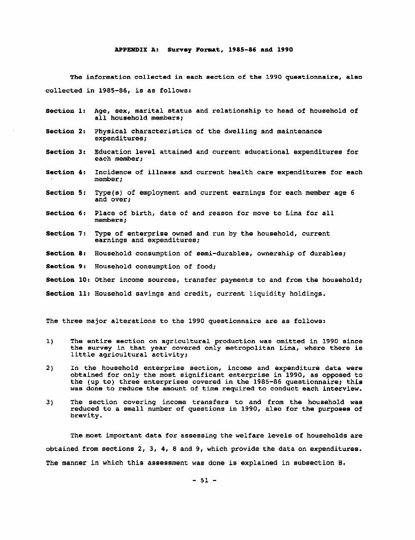
APPENDIX A: Survey Format, 1985-86 and 1990
The information collected in each section of the 1990 questionnaire, also
collected in 1985-86, is as follows:
Section 1: Age, sex, marital status and relationship to head of household ofall household members;
Section 2: Physical characteristics of the dwelling and maintenanceexpenditures;
Section 3: Education level attained and current educational expenditures foreach member;
Section 4: Incidence of illness and current health care expenditures for eachmember;
Section 5: Type(s) of employment and current earnings for each member age 6and over;
Section 6: Place of birth, date of and reason for move to Lima for allmembers;
Section 7: Type of enterprise owned and run by the household, currentearnings and expenditures;
Section 8: Household consumption of semi-durables, ownership of durables;
Section 9: Household consumption of food;
Section 10: Other income sources, transfer payments to and from the household;
Section 11: Household savings and credit, current liquidity holdings.
The three major alterations to the 1990 questionnaire are as follows:
1) The entire section on agricultural production was omitted in 1990 sincethe survey in that year covered only metropolitan Lima, where there islittle agricultural activity;
2) In the household enterprise section, income and expenditure data wereobtained for only the most significant enterprise in 1990, as opposed tothe (up to) three enterprises covered in the 1985-86 questionnaire; thiswas done to reduce the amount of time required to conduct each interview.
3) The section covering income transfers to and from the household wasreduced to a small number of questions in 1990, also for the purposes ofbrevity.
The most important data for assessing the welfare levels of households are
obtained from sections 2, 3, 4, 8 and 9, which provide the data on expenditures.
The manner in which this assessment was done is explained in subsection B.
- 51 -

APPENDIX B: Construction of Price Deflators
Peru experienced very high rates of inflation from 1985 to 1990. The two
surveys discussed in this paper were conducted from July 1985 to July 1986 and
from June to July 1990. During each of these data collection periods, the price
level also rose substantially. This requires one to construct price indices to
make comparisons of real purchasing power of households both across the two
surveys and within each survey. Controlling for price increases within the 1985
survey was done by Glewwe (1988), the result being that all figures in that paper
were given in terms of June 1985 Intis. For details see that paper. In this
paper all figures, unless otherwise noted, are given in terms of thousands of May
26-June 1 Intis. This appendix explains two things: 1) the calculation of the
price index which compares purchasing power in the month of June 1985 to that in
the week of May 26-June 1, 1990,9 and 2) the method used to control for price
inflation which occurred during the 1990 survey. Appendix E presents some
evidence on whether alternative ways of measuring price inflation would
significantly alter the findings of this paper.
Comparing the 1985-86 data with 1990 data
A price index with a base of June, 1985 was used to construct an "inflator"
allowing the 1985-86 data, which was originally deflated to an average real value
for the month of June, 1985, to be expressed in terms of June 1, 1990 Intis. The
only inflation data for Lima available consistently throughout this period (June,
1985 - July, 1990) is the monthly rate of change in consumer prices. This
information was used to derive a monthly index of prices in Lima from June 1,
1985 to June 1, 1990. Since the 1985-86 survey data is expressed as an averaae
value for the month of June 1985, a geometric mean was taken of the index values
for two periods: 1) June 1, 1985 to June 1, 1990, and 2) July 1, 1985 to June 1,
1990, which resulted in an inflator of 9,182,446. All expenditures from the
9In the text we refer to May 26-June 1, 1990 Intis as June 1, 1990 Intis.
- 52 -
1985-86 deflated survey data were multiplied by this value to derive a real value
in terms of June 1, 1990 Intis. The monthly inflation data used was from Cuanto,
S.A. in Lima, Peru. Monthly inflation data was also available from the Instituto
Nacional de Estadistica (INE), and from Apoyo, S.A. The data from these two
sources both resulted in slightly higher estimates of inflation between June 1985
and June 1990. Therefore the most moderate estimate of inflation, that provided
by the data from Cuanto, S.A., was selected to avoid any overestimation of the
drop in expenditure levels between 1985-86 and 1990 due simply to alternative
methods of collecting price data.
The 1990 Survey Deflators
During the weeks in which the 1990 survey was conducted, the consumer
prices in Lima rose daily at a rate ranging from 1 to 5 percent. The comparison
of real expenditures across households required the construction of three
deflators: 1) a fifteen day deflator, applied to all monetary values for
household expenditures reported for the 15 days up to and including the interview
date; 2) a monthly deflator, applied to monetary values referring to monthly
expenditures (electricity and water bills, for example); and 3) a three month
deflator, for expenditures on services and semi-durables made in the three months
prior to the interview. These deflators allow all nominal expenditure values
collected in the 1990 survey to be standardized according to an index where the
price level on June 1, 1990, equals 1.00. The inflation data used in the
calculation of these indices was collected by Cuanto, S.A., Lima, Peru.
The Fifteen Day Deflator
This deflator was applied to monetary values referring to total
expenditures for food and other frequently purchased goods during the 2 weeks
prior to (15 days up to and including) the interview. Daily inflation rates have
only been calculated in Peru since June 30, 1990, whereas data collection began
- 53 -

June 12, 1990. Therefore, weekly rates of inflation were used to construct a
distinct deflator for each possible date of interview as follows.
A weekly price index (P) was calculated for 10 weeks, beginning two weeks
before the first interview at week 1 (the week of May 26-June 1) and ending with
the final week of interviews, week 10. The inflation rate on which this index
is based measures the total change in the price level from Saturday to Friday.
Weekly Price Index 1
June 1 - August 3, 1990
Week Price Index Inflation Rate (%)(end of week)
Week 1 (May 26-June 1, 1990) 1.00Week 2 1.11 11.2Week 3 1.21 8.9Week 4 1.33 10.1Week 5 1.52 14.1Week 6 1.73 14.0Week 7 1.93 11.5Week 8 2.17 12.4Week 9 2.50 15.1Week 10 3.19 27.6
The 15 day deflator was then determined for each possible interview day,
by taking a weighted average of price inflation on each of the 15 days prior to
(up to and including) the interview date. If these days are denoted as (n),
then the 15 day deflator can be expressed as:
15 day deflator = (P1 x n1) + (P2 x n2) + (P3 X n3) (n+ + n+ n3 = 15)
where (P1) represents the price index for week 1, (nl) represents the number of
days in the fifteen day period prior to the interview which fall in week 1, and
so on. Using the 15 day deflator, all monetary values are deflated to the price
level prevailing on June 1, 1990.
- 54 -

The Monthly Deflator
This deflator applies to monthly household expenditures such as gas and
water payments. Each household reports the last monthly amount paid, and the
month (M) in which the payment was made. The deflator corresponding to each
month (M) is calculated based on an index of weekly inflation where the price
level on June 1, 1990 equals 1.00. An average of this index is then calculated
for the weeks falling in each calendar month, resulting in the following price
index which is also the relevant deflator for each month:
Monthly Price Index
January - July, 1990
Month (1990) Price Index (P) Corresponding Weekly Price Indices
January .26 .24 .25 .26 .28February .34 .30 .33 .35 .36 .39March .46 .41 .45 .48 .50April .62 .55 .62 .66 .68May .87 .74 .82 .87 .92 1.00June 1.29 1.11 1.21 1.33 1.52July 2.08 1.73 1.93 2.17 2.50
The Three Month Deflator
This deflator standardizes monetary values corresponding to total
expenditures for services and semi-durable goods purchased during the thirteen
weeks up to and including the week of interview. Each respondent is asked to
identify the calendar month in which the expenditure was made, or if the good was
purchased several times, the month in which the bulk of the expenditure was made.
This month is referred to as (N) in the discussion that follows.
The deflator was again calculated based on weekly rates of inflation. A
weekly price level index (P) was constructed for the period March 10-July 27,
again setting the price level during the week of May 26-June 1 to 100:
- 55 -
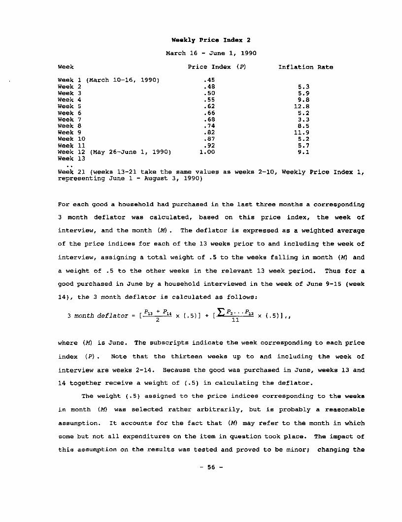
Weekly Price Index 2
March 16 - June 1, 1990
Week Price Index (P) Inflation Rate
Week 1 (March 10-16, 1990) .45Week 2 .48 5.3Week 3 .50 5.9Week 4 .55 9.8Week 5 .62 12.8Week 6 .66 5.2Week 7 .68 3.3Week 8 .74 8.5Week 9 .82 11.9Week 10 .87 5.2Week 11 .92 5.7Week 12 (May 26-June 1, 1990) 1.00 9.1Week 13
Week 21 (weeks 13-21 take the same values as weeks 2-10, Weekly Price Index 1,representing June 1 - August 3, 1990)
For each good a household had purchased in the last three months a corresponding
3 month deflator was calculated, based on this price index, the week of
interview, and the month (M) . The deflator is expressed as a weighted average
of the price indices for each of the 13 weeks prior to and including the week of
interview, assigning a total weight of .5 to the weeks falling in month (M) and
a weight of .5 to the other weeks in the relevant 13 week period. Thus for a
good purchased in June by a household interviewed in the week of June 9-15 (week
14), the 3 month deflator is calculated as follows:
3 month deflator = [13 +14 x (.5)] + P2 x ( 5)],2 11
where (M) is June. The subscripts indicate the week corresponding to each price
index (P). Note that the thirteen weeks up to and including the week of
interview are weeks 2-14. Because the good was purchased in June, weeks 13 and
14 together receive a weight of (.5) in calculating the deflator.
The weight (.5) assigned to the price indices corresponding to the weeks
in month (M) was selected rather arbitrarily, but is probably a reasonable
assumption. It accounts for the fact that (M) may refer to the month in which
some but not all expenditures on the item in question took place. The impact of
this assumption on the results was tested and proved to be minor; changing the
- 56 -

weights even to the extremes of 1 for month (M) and 0 for the other weeks did
not significantly change the results.
- 57 -
APPENDIX C: Calculation of Household Consumption
As stated in Section III of the paper total household consumption consists
of a) explicit expenditures (from Sections 2, 8 and 9 of the questionnaire), b)
the estimated use value of durable goods, and c) imputed rent estimates based on
housing characteristics. The value of explicit expenditures is easily calculated
once appropriate price deflators are derived (cf. Appendix II), but calculation
of the use value of durable goods and imputed rents is more involved. This
appendix explains these calculations for the 1990 data; see Glewwe (1988) for
details regarding the 1985-86 data.
The calculation of the use value of durable goods is based on estimated
rates of depreciation (in terms of value, not just physical condition) of each
good. To estimate the depreciation rate, both the real value of the good when
purchased and at the time of interview is required. Unfortunately, the former
was not collected in the June, 1990, because respondents could not remember exact
prices at the time of purchase due to the rapidly changing price level.
Therefore, depreciation rates based on the 1985-86 data (see Glewwe, 1988) were
used. The rate of depreciation was multiplied py the nominal value of each good
(at the time of the interview) as reported by the household. These values were
then deflated according to the date of interview, applying the fifteen day
deflator (cf. Appendix A) thus expressing the value of each durable good in terms
of June 1, 1991, Intis.
Imputed rents were calculated as follows. All households which rented
their dwellings reported the value of their rental payments, while households
owning their homes reported the value at which they estimated their homes could
be rented. Both of these values were deflated to June 1, 1991 Intis, according
to the date of interview, again using the 15 day deflator. These two deflated
variables were regressed on various characteristics of dwellings, such as the
number of rooms, the materials used to construct the dwelling and the location
within Lima. Standard procedures were used to control for sample selectivity in
each regression but no significant selectivity was found. The regression in
- 58 -

which the dependent variable was the rental value estimated by home owners fit
the data better (in terms of the R-squared coefficient) and was thus used to
assign a rental value to all the households in the sample. Since the dependent
variable was deflated before the regression was estimated, no further deflation
was needed.
- 59 -
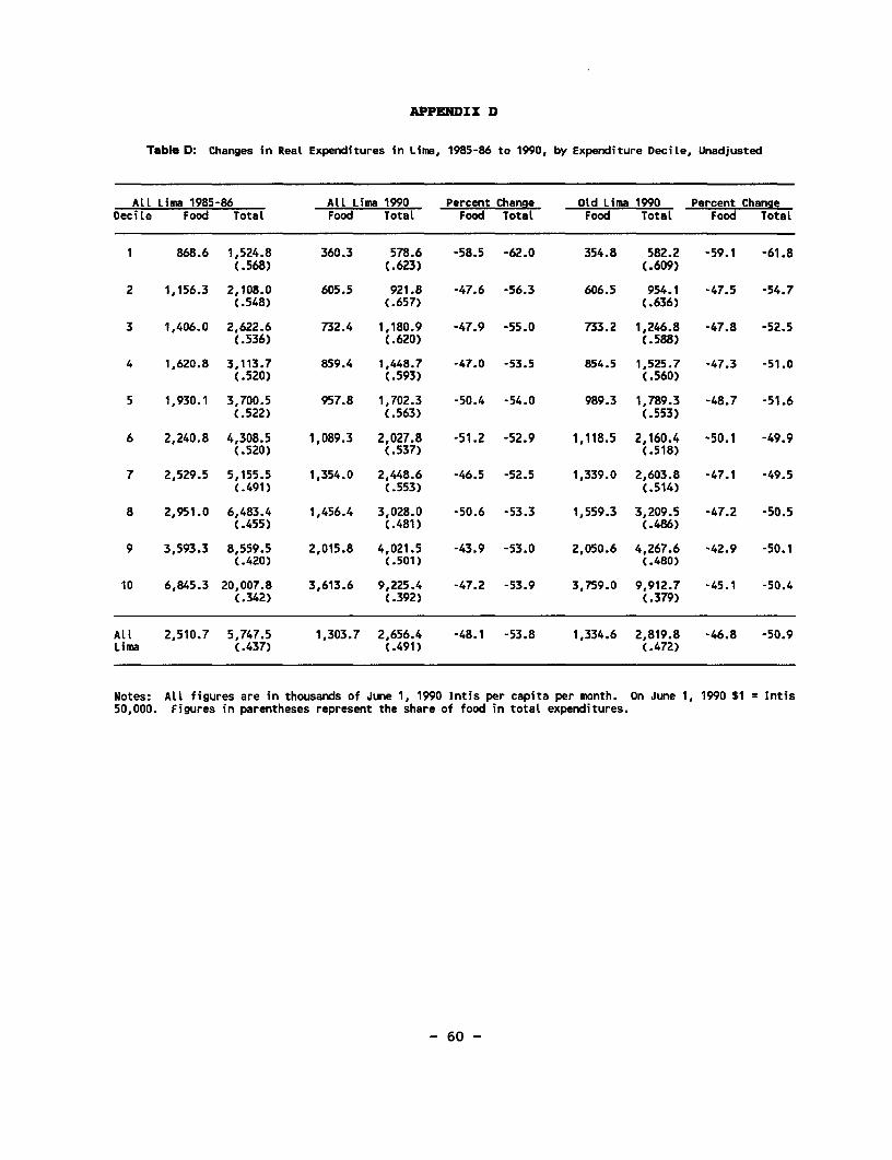
APPENDIX D
Table D: Changes in Real Expenditures in Lima, 1985-86 to 1990, by Expenditure DeciLe, Unadjusted
ALL Lima 1985-86 ALl Lima 1990 Percent Change Old Lima 1990 Percent Change'DeciLe Food Total Food TotaL Food Total Food Total Food TotaL
1 868.6 1,524.8 360.3 578.6 -58.5 -62.0 354.8 582.2 -59.1 -61.8(.568) (.623) (.609)
2 1,156.3 2,108.0 605.5 921.8 -47.6 -56.3 606.5 954.1 -47.5 -54.7(.548) (.657) (.636)
3 1,406.0 2,622.6 732.4 1,180.9 -47.9 -55.0 733.2 1,246.8 -47.8 -52.5(.536) (.620) (.588)
4 1,620.8 3,113.7 859.4 1,448.7 -47.0 -53.5 854.5 1,525.7 -47.3 -51.0(.520) (.593) (.560)
5 1,930.1 3,700.5 957.8 1,702.3 -50.4 -54.0 989.3 1,789.3 -48.7 -51.6(.522) (.563) (.553)
6 2,240.8 4,308.5 1,089.3 2,027.8 -51.2 -52.9 1,118.5 2,160.4 -50.1 -49.9(.520) (.537) (.518)
7 2,529.5 5,155.5 1,354.0 2,448.6 -46.5 -52.5 1,339.0 2,603.8 -47.1 -49.5(.491) (.553) (.514)
8 2,951.0 6,483.4 1,456.4 3,028.0 -50.6 -53.3 1,559.3 3,209.5 -47.2 -50.5(.455) (.481) (.486)
9 3,593.3 8,559.5 2,015.8 4,021.5 -43.9 -53.0 2,050.6 4,267.6 -42.9 -50.1(.420) (.501) (.480)
10 6,845.3 20,007.8 3,613.6 9,225.4 -47.2 -53.9 3,759.0 9,912.7 -45.1 -50.4(.342) (.392) (.379)
ALL 2,510.7 5,747.5 1,303.7 2,656.4 -48.1 -53.8 1,334.6 2,819.8 -46.8 -50.9Lima (.437) (.491) (.472)
Notes: ALL figures are in thousands of June 1, 1990 Intis per capita per month. On June 1, 1990 $1 Intis50,000. Figures in parentheses represent the share of food in totaL expenditures.
- 60 -
APPENDIX E: Use of Household-Specific Price Deflators
Given that prices increased dramatically in Peru between 1985 and 1990, and
particularly because the prices of different items rose by different amounts, one
may question whether using the same price deflator for all households may affect
the results. In particular, if the cost of living for poorer households rises
by a different amount compared to that of wealthier households, should not
different price deflators be used when examining declines in real expenditures
by quintiles or deciles? Theoretically speaking, this objection is valid; one
should use different deflators for different households when relative prices have
changed. However, in practice this may or may not affect one's results. This
appendix examines key results in the text to see whether they change when
household-specific price deflators are used. In general, we find that there are
some small changes but the general findings remain the same.
As conventionally defined (cf. Deaton and Muellbauer, 1980), price
deflators such as the familiar Paasche and Laspeyres indices can be different for
different households only if the shares of expenditures on different items vary
across households and the prices of these different items rise by different
amounts. Perhaps the most obvious example of the former is that poorer
households tend to spend a larger fraction of total expenditures on food,
relative to wealthier households. This is also the case in Lima, Peru (cf. Table
3), and we also find that food prices rose by lower amounts than did non-food
prices from 1985 to 1990.1O
To see whether this change in relative prices brings about substantially
different price indices for households at different expenditure levels, each
household was given a specific price index defined as the weighted shares of the
food and non-food price indices where the weights were each household's food and
loSetting food and non-food price indices equal to 1.0 for June, 1985, thefood price index stood at 6,566.7 on June 1, 1990, compared to 12,068.5 for non-food prices. However, by the end of July, when the last interviews of the 1990survey were taking place, the food index stood at 52,098.5, compared to 62,448.6for the non-food index.
- 61 -

Table El: Means of Household-Specific Deftators, by Expenditure QuintiLes
Quintile Deflator Relative Index
1 9,609.8 100.0
2 9,807.9 102.1
3 9,617.2 100.1
4 9,707.0 101.1
5 10,130.3 105.4
Notes: Deflator is indexed at June 1985 = 1.0. Relative index is normalized at the Quintile 1 deflator.
non-food budget shares." As can be seen from Table E.1, for households in the
first four quintiles the average household-specific price deflators are quite
similar, while that of the wealthiest quintile is about 5% higher than that of
some of the other quintiles (because these households have, on average, the
smallest food shares and non-food prices rose more than food prices). This
suggests that using household specific deflators would have only a relatively
small effect on the results presented in the text of the paper, but to cross-
check this result we present some results comparable to those from Tables 3 and
7 in the text in Tables E.2 and E.3.
Table E.2 shows the decline in real total expenditures by decile in "All
Lima" from 1985-86 to 1990 (expenditure numbers are in 1985-86 Intis). As
before, we find that the poorest decile experiences the steepest decline, and in
fact if we group the households by quintiles (not shown here) we also find that
the poorest quintile experiences the steepest declines. It is interesting to
note that the wealthiest decile experiences the second-largest decline - this
simply reflects the fact that these households have a higher price index because
"A more elaborate method which used price indices and budget shares foreach of 61 items was also used. However, it became difficult to work withbecause although one has price indices on housing for renters (which in Lima roseat a very low relative rate between 1985 and 1990 due to rent control), it wasnot at all clear what price index to use for (imputed) expenditures on housingby home owners, who represent more than half of the population. This led us tosimply aggregate all expenditures into food and non-food.
- 62 -
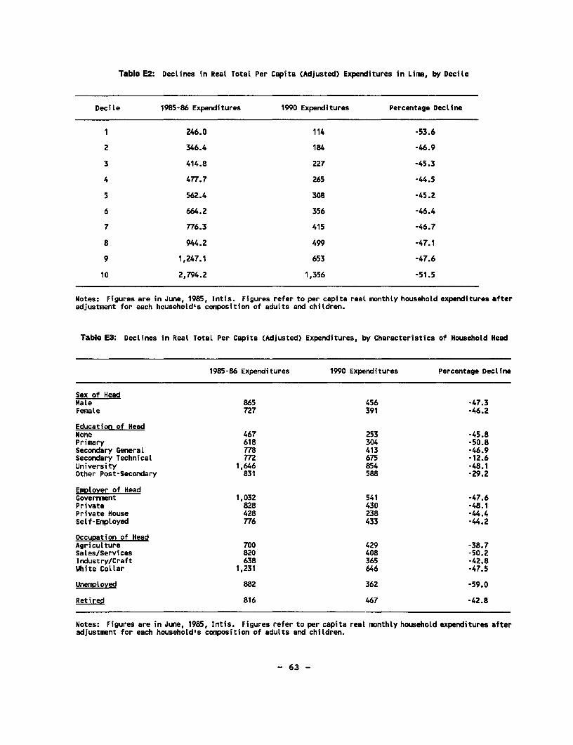
Table E2: Declines in Real Total Per Capita (Adjusted) Expenditures in Lima, by Decile
DeciLe 1985-86 Expenditures 1990 Expenditures Percentage Decline
1 246.0 114 -53.6
2 346.4 184 -46.9
3 414.8 227 -45.3
4 477.7 265 -44.5
5 562.4 308 -45.2
6 664.2 356 -46.4
7 776.3 415 -46.7
8 944.2 499 -47.1
9 1,247.1 653 -47.6
10 2,794.2 1,356 -51.5
Notes: Figures are in June, 1985, Intis. Figures refer to per capita real monthly household expenditures afteradjustment for each household's composition of adults and children.
Table E3: Declines in Real Total Per Capita (Adjusted) Expenditures, by Characteristics of Household Head
1985-86 Expenditures 1990 Expenditures Percentage Decline
Sex of HeadMale 865 456 -47.3Female 727 391 -46.2
Education of HeadNone 467 253 -45.8Primary 618 304 -50.8Secondary General 778 413 -46.9Secondary Technical 772 675 -12.6University 1,646 854 -48.1Other Post-Secondary 831 588 -29.2
Emnlover of HeadGovernment 1,032 541 -47.6Private 828 430 -48.1Private House 428 238 -44.4Self-Employed 776 433 -44.2
Occuoation of HeadAgriculture 700 429 -38.7Sales/Services 820 408 -50.2Industry/Craft 638 365 -42.8White Collar 1,231 646 -47.5
Unemoloyed 882 362 -59.0
Retired 816 467 -42.8
Notes: Figures are in June, 1985, Intis. Figures refer to per capita real monthly household expenditures afteradjustment for each household's composition of adults and children.
- 63 -
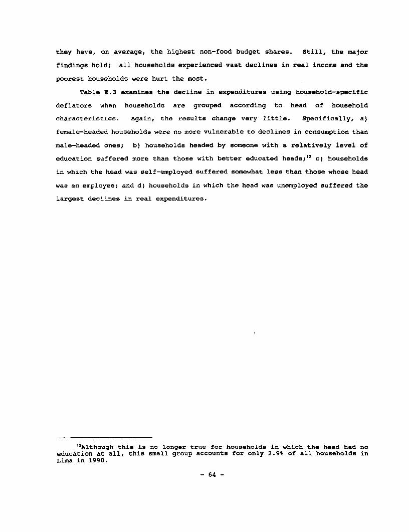
they have, on average, the highest non-food budget shares. Still, the major
findings hold; all households experienced vast declines in real income and the
poorest households were hurt the most.
Table E.3 examines the decline in expenditures using household-specific
deflators when households are grouped according to head of household
characteristics. Again, the results change very little. Specifically, a)
female-headed households were no more vulnerable to declines in consumption than
male-headed ones; b) households headed by someone with a relatively level of
education suffered more than those with better educated heads;12 c) households
in which the head was self-employed suffered somewhat less than those whose head
was an employee; and d) households in which the head was unemployed suffered the
largest declines in real expenditures.
12Although this is no longer true for households in which the head had noeducation at all, this small group accounts for only 2.9% of all households inLima in 1990.
- 64 -

APPENDIX F: List of Geographic Areas
For the purposes of analysis, metropolitan Lima was divided into the
following nine geographic areas. Each area is comprised of the districts as
listed below. The number of households surveyed in each area, selected according
to the population distribution of Lima in 1990, is noted in parentheses.13
1. Cono Sur (2031including Chorrillos, San Juan de Miraflores, Villa Maria del Triunfo,Villa El Salvador, and Lurin
2. Cono Norte (266)including Puente Piedra, Carabayllo, Comas, Independencia, and San Martinde Porres
3. Cono Este (2231including San Juan de Lurigancho, El Agostino, San Luis, Ate, andLurigancho
4. Callao (140)including Callao, La Perla, Bellavista, Carmen de la Legua, and Ventanilla
5. Oeste (961including San Miguel, Magdalena del Mar, Magdalena Vieja, and Brena
6. Centro 1 (40lincluding Jesus Maria and Lince
7. Centro 2 (1891including La Victoria, Lima, and Rimac
8. Centro 3 (651including Santiago de Surco, Barranco, and Surquillo
9. Estrato Alto (591including San Isidro, San Borja, and Miraflores
"3Since the newly settled regions ('New Lima') were oversampled by a factorof two, each household in 'New Lima' receives a weight of (.5) when counting thetotal number of households in each area.
- 65 -

VIII. REFERENCES
Addison, T. and L. Demery. 1985. "Macro-Economic Stabilisation, IncomeDistribution and Poverty: a Preliminary Survey". Overseas DevelopmentInstitute (London), working paper no. 15 (February).
. 1986. "Poverty Alleviation under Structural Adjustment". OverseasDevelopment Institute (London).
Apoyo, S.A. 1990. "Indice de Precios de Apoyo (IPA)". Lima, Peru. (Mimeo).
Arriagada, A.M.. 1989. "Occupational Training Among Peruvian Men: Does It Makea Difference?" Policy, Research and External Affairs Working Paper No.207. The World Bank. Washington, DC.
Conway, Patrick. 1991.' "How Successful is World Bank Lending for StructuralAdjustment". Policy, Research and External Affairs Working Paper No. 581.The World Bank. Washington, DC.
Cornia, Giovanni, Richard Jolly and Frances Stewart. 1986. Adiustment With aHuman Face. Oxford University Press.
Cuanto, S.A. 1990. "Costo Diario de una Canasta de Alimentos que SatisfaceRequerimientos Nutricionales Recomendados por el Instituto Nacional deNutricion". Documento de Trabajo. Lima, Peru. (Mimeo).
_ 1990. "Inflacion Semanal por Grupo de Consumo". Lima, Peru. (Mimeo).
Deaton, A.S. and J. Muelbauer. 1980. Economics and Consumer Behavior.Cambridge University Press.
_ 1986. "Measuring Child Costs in Poor Countries". Journal ofPolitical Economy, volume 94, pp. 720-44.
Dornbusch, Rudiger, and Sebastian Edwards. 1990. "Macroeconomic Populism".Journal of Development Economics. Volume 32, No. 2 (April).
Foster, James and Anthony Shorrocks. 1988. "Poverty Orderings." Econometrica,Volume 56, no. 1, pp. 173-77.
Glewwe, Paul. 1988. "The Distribution of Welfare in Peru in 1985-86." LivingStandards Measurement Study Working Paper No. 42. The World Bank.Washington, DC.
Grooteart, Christiaan, and Ana-Maria Arriagada. 1986. "The Peruvian LivingStandards Survey: An Annotated Questionnaire". Education and TrainingDepartment. The World Bank. Washington, DC.
Instituto Nacional de Estadistica. April 1988. Encuesta Nacional de HoaaresSobre Medicion de Niveles de Vida ENNIV (1985-1986): Analisis deResultados. Direccion General de Censos y Encuestas. Lima, Peru.
International Monetary Fund. 1980-1990. International Financial Statistics.Bureau of Statistics. Washington, DC.
Kanbur, Ravi. 1987. "Measurement and Alleviation of Poverty with an Applicationto the Effects of Macroeconomic Adjustment". IMF Staff Pacers, 34(l):60-85.
Kakwani, Nanak, Elene Makonnen and Jacques van der Gaag. 1990. "StructuralAdjustment and Living Conditions in Developing Countries". Population andHuman Resources Department Working Paper No. 467, World Bank.
- 67 -
Killick, T. (ed.). 1984. The IMF and Stabilisation: Develo-ina CountryExperiences. Heinemann Educational Books (London).
Lago, Ricardo. 1991. "The Illusion of Pursuing Redistribution ThroughMacropolicy: Peru's Heterodox Experience 1985-90". The Macroeconomics ofPopulism in Latin America. Dornbusch, Rudiger and Sebastian Edwards(eds.) University of Chicago Press, forthcoming (November 1991).
Paus, Eva. 1991. "Adjustment and Development in Latin America: The Failure ofPeruvian Heterodoxy, 1985-1990." World Development, volume 19, no. 5,pp. 411-434.
Ravallion, Martin. 1991. "Reaching the Poor through Public Employment:Arguments, Evidence and Lessons from South Asia". The World Bank ResearchObserver, volume 6, no. 2, July. World Bank, Washington, DC.
Taylor, Lance. 1988. Varieties of Stabilization Experience: Towards SensibleMacroeconomics in the Third World. Clarendon Press. Oxford.
Thorp, Rosemary. 1987. "Politica Economica y Planificacion de Largo Plazo en elModelo Heterodoxo". Instituto Nacional de Planificacion. Lima, Peru(Mimeo).
United Nations. 1980-88. Estudio Economico de America Latina v el Caribe. NewYork.
Webb, Richard and Graciela Fernandez Baca. 1990. Peru en Numeros 1990. CuantoS.A. Lima, Peru.
World Bank. 1990. World Development ReDort. Oxford University Press. NewYork.
- 68 -

Distributors of World Bank PublicationsARGENTINA FINLAND XUWAIT SOUT AFRICA, BOTSWANACaro Hisdi SRL AkPO in, 2 k3 ppo MEMsRBBumtSenv SOUIH i TGalatacGuea P0 Box 128 P0 Box546S Oolod UnerityPressFloda 154h65 41OfRk 453/465 HdInO 10 oUthenUy 1333 BuemnAie F0101 MALAYSIA Po Bx 1141
Umva.ydMalayaCooeeative C5PeTowwAUSTRALIA, PAPUA NEW CUINEA. p imedFIJI, SOLOMON ISANDS, FRANCE P O Box ll m i ted RamVANUATU, AND WESTERN SAMOA Word Bank Publicatios jD.A 6m6. 4avenue d'1enI6lensSPionS40964dWhl o I dWa 75116 Pris MEXCO CPO.oxt109Machlam 3132 C*Gs-am 313Z CERMANY INFOaEC Jcha urg 2B24
ULNO.Voag 14060Tl lPyM Jco SPAINAUSTRIA PppdilPwdo lrbroleeSGerd and Co D-533C Sia I MOROCCO Cateato 37Grabao31 SodftA d'Ead M neg Maca 2 MadAA1(tl WI GREECE 122u01tddd`Anfd
In CMb= tabresis Iotmusioosl AEIXSBAHRAIN 24. ppodaramaSt rPaNPasi Ccm , de Can 391Bkran Reamch and Conultny Atlwe s,11635 NETHERLANDS C -oedoaC31
A_odat Lid DeLUndebojbIwnOrFPublV0ati0oerad BSddIn No. 42 GUATEMALA 5SRI LANA AND THE MAIDIV7S
PD.Bpk N SA brdaleSdraSant 74HDAE H Hsbrog L ck 1 Home BookokhpMarm Toawn 317 Zaal NEW ZEALAD BO W244
GuateitaiuCty HMoELry and lfoonmSvi I,S adterMpvzm ABANGLADESH .,, CardiwMawatMid. Indu Dtinflevel_pmut HONG KONG. MACAO Na CdMomto 2
AasssmaSadckelyMDAS) Ana 2lE LId. Adm WHowe S, Road 16 4A4eWaD dLamd. d SWWED
mondR / W C tre NIGERIA Fmrtosdk oDhaka 1209 2nd Hoar Un mi .yP is mited Reg.,npgtot 12. Ba 163
B 1~~~~~~~~~~~~~-rlHgTreeCrovnaiutmjdddgtaih S-10327StoddtaimBmut hb vateMailRaM951IoNrAhtmedSarek INDIA lbadMou %4t5 Aled Pu sh Ltd.n Fe Priavat. ordd
751 MountRoad NORWAY Wernmagxat-WillamaAN KDA Avenue ~~madmu-6003 BNO3WA4
76,KuDAh Aentoota Nrme, ebdOrshon Cantor S-10425StodchlmBook Dnepn tm
BELGIUM ISJtJ HerM PO Box Q25ersEaXd SWITZERLANDBELGIUM ~~~~~~~~~~15j.N.HerediaMarg N-OWl (mo 6 Poeo.Sk t)k.Jean De i.noy Ballard Eerate Lbsane PayotA, du Rd 2i B2ntbay -400 VB OMAN U rw Pus,
ID60 Bruwd. MEMRB hiknmdm Services Case,S prue Ca 38uIC60 Brussels 13/14 Aaf AU Road PO Box 1613, SabArport CHI, 1 Genes11
CANADA Nev hdih-1100O2 Muro 1tLeDdLubbrCrP. 85, IlSeueAmpire 17 ChittaranmomAvwiue PAKISTAN Fobrai P5yotBoucku4l QO4bC Cakutt. - 7VD 072 MirsBooxAge.y life Ayot ent
CHBSEA JaydevaHoelidlding P0 Box No 729 CHI02lausLaneCHINA MthMnn Rod GdnAr Lo3Chon einaF al & Eoomac B"aeloe f5603TZ9
Pubisihng House PERU OxfAdZAuNversityPS.D. FoSiDto,gJie 3-5-1129 Kaddgud Crows Road PEdtrUa eroaS POid UBiOtt9P9Bs$ng Hyderbad -E SW 7 Apartado 1324 D.-Sazam
COLOMBIA Prartsna Flats, 2od FloorInfoenlsor Ltd-. NearThakere BugNawanwaL N C THAILANDAprtsdo Ameo 34270 Alunad bd-380009 ]etaic o r C6ntRadnBogota ox Fift Flos, r o feIn .1 1ding. Bk
COTE D'IVOIRE ;16.Aa House Ayala Avenue MakaICodeed'Editin*etdeDtfsuion LucIno,e -22601 Oero MmD TRINIDAD TOSAGO, ATIGUA
Ahicau,(CEDA) BARBUDA, BARBADOS,04BP. 541 LNDONESIA UDOMNICA. GRENADA, GUYANA,
Abidl n04PiO Pt. Indira iSmited PORTUJGAL JAMAICA, MONTSERRAT, ST.Abidpn 04 Plateau LInu Rothd.g Uwasua Patg KrrTS & NEVIS. ST. LUCIA.CYPRUS PO BoR1l8 RuD. Carma074 ST. VINCENT l GRENADINESMEM(RB infornationSeic, 5aka-rt PUt 120D Lasho Syatanaba Sd UnitPO Box 20 ADIAAIA AA 49 Watts5SteetNO o,aa 1 IRAEL SAUDIARABLA,QATAR C-,?pe
Naors IYozmoLterre Ud POBokS3ree Trlaudad, WeaIndia
PO ~P0 Box 305Riah1961UNE RA M3AEDENMARK PP Box SfD55S mfusn"udLtto"ur TdtAviv61560 Rty 1IIIUNITEDARABIEMIRATESRoooAAlle laml MEMR inf ionServic P0 Box W97DK1970 Fredelibal; C ITAL Y St-ryh
DOMINICAN REPUBLIC UcM C _os arn. Sar.nn SPA Al Al" N KGEdAhmTallorer- porrA. AlucDi Dahas CVIt F NrrED KINGDOMEditors TaIIoc C. por A. ~~~Vi Dora Di Calabno,s 1/1 Firs Flo M.-coofo EAdResaatron e lsaba Is Ct6lca 309 C0 Postal 552 r o 7Y Po Box 3ApadoPo" l2190 53125Florece Riydl Alton,N impshIceGU342PGSanto Domingo
JAPAN Ha#AbdullhAbreA BuldingEGYPT, ARAB REPUBLIC OF Eaten Book Semvce r Bo.etAl Abratm 374. Hego 34asou,e Bukyo.k 113 PO B__39 VEiNEZUELAAl Gal Seet Tokyo Ubre Aptdo. t0 e
KENYA 33,Mohammd Hinm Awad Ste Carsca 1060-AThe Middle East Obsver Afnca Book Semvle(EA)Ad Po Box 197841 Shrif Stree P.0 Bo 45245 Jedd hCAM Nairobi
EL SALVAi7R KOREA, REFVBUC OF SINGAPORE,TAIWAN,EL"d SLAOKOE.RPICOFMYAN1.AE.BRUNEIPuaadaa Pa; Kore Book Caicratin lnf abn PublicaionAvuida ManuaEnnqpaeArz 8353 Po Box 101, KvangwfubmmovanUd.EdificaoSISA,Iol Pbao Seo02u06 ltHF. Pei- IndutrnalSan Salvado Bldg.
24 New Indulal RoadStga.p,r 19p53

LSMS Working Papers (continued)
No. 51 Child Anthropometry in Cote d'Ivoire: Estimates from Two Surveys, 1985 and 1986
No. 52 Public-Private Sector Wage Comparisons and Moonlighting in Developing Countries: Evidencefrom C6te d'Ivoire and Peru
No. 53 Socioeconomic Determinants of Fertility in Cote d'Ivoire
No. 54 The Willingness to Pay for Education in Developing Countries: Evidence from Rural Peru
No. 55 Rigidite des salaires: Donnees micro6conomiques et macroeconomiques sur l'ajustement du march6du travail dans le secteur moderne (in French only)
No. 56 The Poor in Latin America during Adjustment: A Case Study of Peru
No. 57 The Substitutability of Public and Private Health Care for the Treatment of Children in Pakhstan
No. 58 Identifying the Poor: Is "Headship" a Useful Concept?
No. 59 Labor Market Perfonnance as a Detenninant of Migration
No. 60 The Relative Effectiveness of Private and Public Schools: Evidence from Two Developing Countries
No. 61 Large Sample Distribution of Several Inequality Measures: With Application to C6te d'Ivoire
No. 62 Testing for Significance of Poverty Differences: With Application to C6te d'lvoire
No. 63 Poverty and Economic Growth: With Application to Cate d'Ivoire
No. 64 Education and Earnings in Peru's Informal Nonfarm Family Enterprises
No. 65 Formal and Informal Sector Wage Determination in Urban Low-Income Neighborhoods in Pakistan
No. 66 Testingfor Labor Market Duality: The Private Wage Sector in Cote d'Ivoire
No. 67 Does Education Pay in the Labor Market? The Labor Force Participation, Occupation, and Earningsof Peruvian Women
No. 68 The Composition and Distribution of Income in C6te d'Ivoire
No. 69 Price Elasticities from Survey Data: Extensions and Indonesian Results
No. 70 Efficient Allocation of Transfers to the Poor: The Problem of Unobserved Household Income
No. 71 Investigating the Determinants of Household Welfare in C8te d'Ivoire
No. 72 The Selectivity of Fertility and the Determinants of Human Capital Investments: Parametricand Semiparametric Estimates
No. 73 Shadow Wages and Peasant Family Labor Supply: An Econometric Application to the Peruvian Sierra
No. 74 The Action of Human Resources and Poverty on One Another: What We Have Yet to Learn
No. 75 The Distribution of Welfare in Ghana, 1987-88
No. 76 Schooling, Skills, and the Returns to Government Investment in Education: An Exploration UsingData from Ghana
No. 77 Workers' Benefits from Bolivia's Emergency Social Fund
No. 78 Dual Selection Criteria with Multiple Alternatives: Migration, Work Status, and Wages
No. 79 Gender Differences in Household Resource Allocations
No. 80 The Household Survey as a Tool for Policy Change: Lessons from the Jamaican Survey of LivingConditions
No. 81 Patterns of Aging in Thailand and Cote d'Ivoire
No. 82 Does Undernutrition Respond to Incomes and Prices? Dominance Tests for Indonesia
No. 83 Growth and Redistribution Components of Changes in Poverty Measure: A Decomposition withApplications to Brazil and India in the 1980s
No. 84 Measuring Incomefrom Family Enterprises with Household Surveys
No. 85 Demand Analysis and Tax Reform in Pakistan

The MForld Bank
Headquarters European Office Tokyo Office1818 H Street, N.W. 66, avenue d'16na Kokusai BuildingWashington, D.C. 20433, U.S.A. 75116 Paris, France 1-1, Marunouchi 3-chome
Chiyoda-ku, Tokyo 100, Japan Telephone: (202) 477-1234 Telephone: (1) 40.69.30.00 hFacsimile: (202) 477- 6391 Facsimile: (1) 40.69.30.66 Telephone: (3) 3214-5001Telex: wLi 64145 WORLDBANK Telex: 640651 Facsimile: (3) 3214-3657
RCA 248423 WORLDBK Telex: 26838Cable Address: INThAFRAD
WASHINGTONDC