Embed Size (px)
Citation preview

Série Textos para Discussão
Poverty and Environmental Degradation: the KuznetsEnvironmental Curve for the Brazilian Case
Fabio Granja e BarrosAugusto F. Mendonça
Jorge M. NogueiraUniversidade de Brasília
Texto no 267Brasília, dezembro de 2002
Universidade de BrasíliaDepartamento de Economia
Department of Economics Working Paper 267University of Brasilia, December 2002

UNIVERSIDADE DE BRASÍLIA
DEPARTAMENTO DE ECONOMIA
TEXTO PARA DISCUSSÃO No 267
Poverty and Environmental Degradation: the Kuznets Environmental Curve for the Brazilian Case
Fabio Granja e Barros
Augusto F. Mendonça
Jorge M. Nogueira
Universidade de Brasília
Brasília, 20 de dezembro de 2002
Fabio Granja e Barros, Augusto F. Mendonça e Jorge M. Nogueira, 2002

UNIVERSIDADE DE BRASÍLIA
DEPARTAMENTO DE ECONOMIA
Campus Universitário Darcy Ribeiro
Instituto Central de Ciências
Caixa Postal 04302, 70910-900 Brasília, DF, Brasil
Tel.: (55-61) 3072498, 2723548
Fax: (55-61) 3402311
E-mail: [email protected]
http://www.unb.br/ih/eco
Chefe do Departamento
Prof. Jorge Madeira Nogueira
Sub-Chefe do Departamento
Prof. Rodrigo Peñaloza
Coordenador de Pós-Graduação
Prof. Paulo César Coutinho
Coordenador de Pesquisa e Extensão
Prof. Maurício Soares Bugarin
SÉRIE DE TEXTOS PARA DISCUSSÃO
Comissão Editorial, mandato junho de 2001 a fevereiro de 2003
André Rossi de Oliveira
Bernardo Mueller
Flávio Versiani
Jorge Nogueira
Maurício Bugarin (editor)
Mauro Boianovsky
Apoio: CESPE UnB
1
Poverty and environmental degradation: the Kuznets Environmental Curve for the Brazilian case
Fabio Granja e Barros, Augusto F. Mendonça
e Jorge M. Nogueira
Abstract
The theory relating environmental degradation and a certain level of per capita income of a
country is known as Environmental Kuznets Curve (EKC). This theory is based upon an
environmental demand that would increase social control and government regulations as a
society gets richer. However, little has been said about the variation of this theory in countries
with great poverty and low level of education. The objective of this paper is to investigate if
Brazilian poverty affects the EKC. We handle models involving dichotomous response
variables to investigate if social and economic indicators - mainly income and education -
affect the environmental demand and consequently the EKC. Our results permit to infer that
increases in education level and of some social indicators can generate higher probabilities of
changes on individual demand for environmental goods and services. These results can be
disaggregated into three interesting findings: i) the Brazilian social problems - represented by
low levels of education and of income – has affected demand for environmental goods and
services and, consequently, the EKC; ii) the direct relationship between poverty and
environmental degradation, as some international institutions have tried to stand out, does not
seem to be so consistent; investments on education and on some basic services would increase
demand for environmental goods and services even among the poorest sections of society; and
iii) investments on social areas could guarantee an economic growth with low levels of
environmental degradation, generating a “tunnel” in the EKC.
Key Words: Theory of the Environmental Kuznets Curve (EKC), economic growth,
Brazilian social problems, environmental demand, models involving dichotomous response
variables, social and economic indicators.
Category JEL: Q10 and O10

2
• Initial Comments
The relation between income level and environmental quality has been widely debated inside
academic circles. There is no a priori reason to assume this relationship to be strictly
monotonic. Actually, environmental quality may worsen with income within some ranges of
income, but improve over others. Also, no one should expect the same relationship to hold for
all dimensions of environmental quality (Boyce and Torras, 2002). Empirical evidences have
stressed that environmental health will depend, among others factors, upon the development
stage achieved by a given country. In its initial stages, a country is dependent upon agriculture
and primary mineral resources with relative small pollution impacts.
As income of a country continues to grow with economic development, manufacturing
production achieves larger share of national domestic production. In general, industrialisation
starts with light industries (e.g. textiles) moving toward a phase of heavy industries (e.g.
steel). This is a phase of medium level income, of increasing use of natural resources and
intensification of environmental degradation. Finally, the development phase overcomes
industrialization with services enlarging its share of national domestic product, while
industrial share stabilizes. In this stage, it is observed a reduction of raw material utilization.
However, it is also observed an increase on waste generation per unit of production.
It is in this context that the Environmental Kuznets Curve (EKC) arises1. The basic idea is
quite straightforward: environmental pressure would decrease after certain level of economic
development. We suggest that the main deficiency of the modelling sustaining EKC is that
one does not observe clearly why the increase in income influences reduction of
environmental degradation caused by any pollutant. Researchers have different arguments
about possible elements that may correlate these variables. Some of them believe that
environmental quality improvement occurs naturally with the process of economic
development. In other words, environment improvement is endogenous to the process.
However, others stress that an improvement in environmental indicators is a result of
increasing demand for environmental quality. This demand grows with rising income and put
1It is also known as the “U” inverted curve.
3
pressure upon policy makers for more regulations and investments on environmental areas
[EKINS (1997) and MUNASINGHE (1998)].
In spite of this lack of consensus on cause-effect relationship between income and
improvement of environmental indicators, the great majority of scholars agree about the
elements that act degrading the environment. It can be argued that degradation is related with
scale, composition and technological effects [GROSSMAN & KRUEGER (1995)]. These
effects relate themselves, respectively, with the increase of economic activity, with
consumption and production structures and with adopted technological pattern. If the
degradation intensity were constant among countries, one would expect that, by the scale
effect, an increase in production of all them would increase environmental degradation at the
same rate in the whole planet.
However, the scale effect could be reduced if composition and technology effects were
sufficient intense to act in the opposite direction. Therefore, degradation could be reduced
with economic growth as long as production would be transferred between sectors. This
would be the case if the service sector would increase its participation relatively to the
manufacturing sector. Another possibility would be changes in the consumption structure
enabling a reduction in waste generation, for example. Moreover, some sectors could adopt
technologies that would use less natural resources and that would pollute less.
Furthermore, GROSSMAN & KRUEGER (1995) themselves suggested that “an induced
policy response” in the form of more stringent and more strictly enforced environmental
standards, driven by citizen demand, has provided the strongest link between income and
pollution. Following this reasoning, BOYCE & TORRAS (2002) investigated possible causal
linkages between changes in income level and changes in pollution levels. These authors also
pointed out that this connection hitherto remarkably absent from discussions of the EKC.
Our research is one of very few studies to deal with the EKC in a context of a poor and
unequal society2. The vast majority of EKC studies have been based upon countries where
2 Some countries present an enourmous social inequality. That is, there is a large difference among income levels, without having a significant number of poor people. However, the brazilian social reality presents a high level of poverty together with a high social inequality.
4
poverty and low level of education was not part of their reality. We argue that, the “poverty
cycle”3 of some countries, like Brazil4, could change in the EKC's rationale. In a reality like
this, it is possible, we argue, that the turning point where pollution would start declining can
be higher than in a different social reality. Even more, the turning point may never exist. This
could happen due to the fact that high levels of poverty may change preferences and,
consequently, the demand for environmental services.
In such a context, some linkages that could explain the EKC would become biased, because
the neediest portion of the population would be more concern in achieving their basic needs.
Nevertheless, some key socio-economic variables, mostly education, may suggest that public
investments in education and basic services may change the demand for environmental goods
and services of a country and, thus, reduce the potential of degradation. Our results show that
there is not a direct relation between poverty and environmental degradation, as some
international institutions have frequently emphasised.
This research has, therefore, as its main goal to investigate whether the Brazilian social
problem – manifested, among other factors, by a high concentration of income and by a low
average educational level – can affect demand for the environment and, thus, a theoretical
EKC. There is another relevant objective of this research. Besides to inquire whether the
existence of a widespread poverty will put doubt upon the explanatory power of the ECK
theory for the Brazilian reality, we also show evidence of a necessary interaction among
socio-economic and environmental policies.
A frequently used indicator to evaluate EKC in developing countries is the deforestation rate.
This indicator of environmental degradation expresses directly individuals' demand for
environmental goods and services. In other words, the decision to conserve a forest areas
eliminates any other type of alternative use of this natural resource. Thus, the use of
3 Brazil presents a high level of poverty represented by a great number o people living with low levels of income and of education. 4Brazil is a relevant case study for a research about the EKC. In spite of being one of the biggest economy among all countries, Brazil has not yet arrived at a level of high environmental degradation. The countryu detains one of the largest reserves of natural resources in the whole planet, being object of constant international pressures. On the other hand, Brazil has one of the worst income distributions of the world, better only of those of some African countries. This combination of factors

5
deforestation rates as indicators of environmental conservation enables us to test the relation
between low levels of income and of education with the demand for environmental goods and
services, and then with the EKC.
In order to do so, we use a data base generated through a contingent valuation method to
check the relevance of socio-economic variables in the demand for environmental goods and
services provided by the Carajás Region, in the Brazilian Amazon. These data reflect the
willingness to pay to avoid further exploitation of mineral reserves of Carajás Region. We
have used them to test two hypotheses: 1) socio-economic variables – mostly income and
education – affect demand for environmental goods and services; and 2) the variable
education is also significant in shaping the demand for environmental goods and services by
those people who are willing to pay for conservation, but they do not have enough income to
do so.
Econometric models with dichotomous dependent variable – Logit and Probit – are used to
analyse whether these variables influence demand for environmental services. The paper has
two main sections. The next section deals with evidences of the EKC, through a survey of
theoretical studies. The second section presents our econometric results, as well as highlights
consequences of our results for the EKC theory and for future public policies.
• Income Level and the EKC.
In a well known study, Munasinghe (1998) show how the willingness to pay (WTP) for an
environmental good or service is influenced by income and by the level of environmental
understanding of an individual. Actually this relationship was also exploited by LOPEZ
(1994). For him, if producers do not pay for the pollution that they impose to the society, then
an increase in production will invariably increase the pollution level. However, when these
same producers pay the marginal social cost of pollution5, then the relationship between
emissions and income would become directly dependent of technology and of preferences.
guarantees to Brazil a relevant position in the discussion of the relation between poverty and the environment. 5In other words, they incorporate in their costs the social damages of pollution.
6
If the preferences are homothetic, an increase in production would also generate an increase in
the pollution level. However, when preferences are not homothetic, as is usually the case in
most actual situations according to POLLAK & WALES (1992), changes in pollution due to
economic growth depends upon the elasticity of substitution in production between pollution
and inputs, as well as the degree of agent aversion to risk (that is, rate of marginal reduction
of utility in the consumption of produced goods). As much larger the rate of decreasing
marginal utility and the substitution in production, smaller should be the increase in pollution
due to increments in production.
In this context, pollutants as the SO2, that are controlled in many countries, would may have
their effective price close to the optimum level. In these cases, the “U” inverted relation to
income should occur. However, CO2 effective price is, probably, far from the optimum level,
evidencing a monotonic relation in the EKC. This may be happening due to a low elasticity of
substitution and to the fact that the environmental damage is less evident, implying in an
higher turning point in the EKC.
SELDEN & SONG (1994), however, have derived a “U” inverted curve by means of a
“optimum path for pollution”, using a model of growth and the environment proposed by
FOSTER (1973). Actually, this model is similar to that by LOPEZ (1994), but adding the
hypothesis that utility is additive in consumption and pollution. While LOPEZ (1994) and
SELDEN & SONG (1994) haved developed models based on agents with infinite time span,
JONHN & PECCHENINO (1994) develop an overlapping generation model, where pollution
externalities have been generated more by consumption than by production activities. A
pollution consumption model was proposed by McCONNELL (1997). He proposed that
income elasticity of demand for environmental goods not necessarily defines any rule for
EKC Model. In other words, pollution level could decrease even though elasticity were not
positive.
In order to allow for better visualization of income and eduaction level upon willingness to
pay (WTP) for environmental goods, the following model provides evidences on how these
variables explain endegenously the EKC. In this model, the economy is perfectly competitive,
at first. In a second stage, it consideres some market imperfections. Suppose that an individual
7
or a firm, in a certain country, wishes to maximize net benefits, in a situation where both
benefits and costs are dependent of income level and of environment quality, that is:
),(),(max YECYEBBL −= (1)
where BL representes the net benefit to be maximized, while B and C are, respectively,
benefits and costs. Both are function of the level of environmental degradatrion (E) and of
income per capita (Y).
In any income level, individual wishes to maximize BL at the level where
marginal benefit, or the willingness to pay for a certain environmentalk quality, is equal to
marginal cost to obtain that level of environmental quality. The first order condition will
garantee:
0=− gg CMBM (2)
where EBBM g ∂∂= / and ECCM g ∂∂= / . A key aspect of this present research is , as
mentioned before, to analyse how the equilibrium (in the point −)*,( YE ) is affected by
changes in income. Thus differentiating in relation to income, we have:
0)/()/( ** =∂∂−−∂∂+ == EEgegyEEgegy YECMCMYEBMBM (3)
where iBMBM ggi ∂∂= / and iCMCM ggi ∂∂= / for i=Y, E.
Equation (3) relates (E) and (Y) at the level where environmental degradation (E*) is
optimized for any income level. Thus, we have:
8
)/()()/( * gEgEgygyEE BMCMCMBMYE −−=∂∂ = (4)
This equation shows that the sign of )/( YE ∂∂ , according to the inverted “U” curve model,
changes from positive to negative at a given level of income. Therefore, the sign of
enviornmental degradation elasticity in relation to income per capita changes from positive
to negative as income grows.
It can be verified from equation (4) that it is reasonable to represent the WTP for
environmental improvements by a curve of positive coefficients, that is 0>gEBM . This
explains why points representing higher levels of environmental degradation will have higher
willingness to pay for an improvement in environmental quality. Furthermore, a curve of
marginal cost for reverting environmental degradation has negative coefficient, that is,
0<gECM . This is explained as sucessive reduction in the level of environmental degradation
will have increasing costs. For this reason, it is possible to say that the denominator of
equation (4) will become negative and that the sign of expression ( YE ∂∂ / ) is opposite to the
sign of numerator ).( gYgY CMBM − Now it is necessary to analyse signs of the numerator.
These environemnatl goods have income elasticity higher than normal market goods
[BATEMAN et al. (1992)]. Further, due to unicity, these goods have a low elasticity of
substitution.
The superior section of Figure 1 shows that gBM and gCM curves vary parametrically
with income increases. Thus, at low levels of development and income, )( 0YBM g and
)( 0YCM g intercept themselves at F.
Figure 1: EKC Behaviour
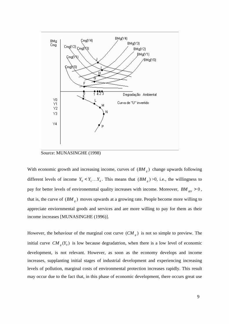
9
Source: MUNASINGHE (1998)
With economic growth and increasing income, curves of )( gBM change upwards following
different levels of income 410 YYY h< . This means that )( gBM >0, i.e., the willingness to
pay for better levels of environemntal quality increases with income. Moreover, 0>gyyBM ,
that is, the curve of )( gBM moves upwards at a growing rate. People become more willing to
appreciate enviornmental goods and services and are more willing to pay for them as their
income increases [MUNASINGHE (1996)].
However, the behaviour of the marginal cost curve )( gCM is not so simple to preview. The
initial curve )( 0YCM g is low because degradatrion, when there is a low level of economic
development, is not relevant. However, as soon as the economy develops and income
increases, supplanting initial stages of industrial development and experiencing increasing
levels of pollution, marginal costs of environmental protection increases rapidly. This result
may occur due to the fact that, in this phase of economic development, there occurs great use

10
of natural resources and generation of pollution, with little use of knowledge and technology
to save the environment.
Therefore, 0>> gYgY BMCM when (Y) is low. However, with continuing economic
development and with a country achieving the post-industrial phase, both available human
resources and improved technological knowledge reduce environmental marginal abatement
and protection costs with higher levels of income (technology effect). Another factor may be
related with structural changes in the economy, with the service sector becoming responsible
for a larger portion of a country’s national gross product (composition effect). In a context
like this, gYCM shows a tendency to reduce with the increase in income and with a larger
“environemntal consciousness”, i.e., 0<gYYCM .
All these arguments are to show that )( gYgY CMBM − would be positive in initial stages of
economic development, but would become negative after a given level of income is achieved.
Curves gBM e gCM intercepts at the equilibrium points F, G, H, I and J corresponding to
maximization points of equation (2). Respective ordering pairs ),( ii YE with i=0 a 4, define
points K, L, M, N e P that form the EKC. Thus, changes in gBM and gCM curves show
the result of this process upon the “U” inverted curve. (See the lower portion of Figure 1) .
In a cenario of competitive equilibrium, as described above, the Parentian optimum garantees
that level of environmental degradation is the socially desirable in the whole curve. However,
it is possible to identify situations where imperfections in the economy can provide a non
optimum pattern or economically inefficient. Therefore, private gBM e de gCM curves,
based on which consumers and producers choose, may differ from the social optimum curve,
resulting in a degradation level higher than the socially desirable.
Market failures may affect the demand for environmental quality ( gBM ). Lack of information
about consequences of environmental degradation upon human health and well-being may be
result of low educational level. This can result in a low willingness to pay by consumers.
Social groups with low levels of education may be directly exposed to pollution and, as

11
consequence, they may be not aware of damages being caused to their health. If this were the
case, the increase of ( gBM ) curve would happen at a lower rate, even when income increases.
The final result of this process would be a degradation level higher than the social optimal.
There could be another environmental consequence of low educational level. Some economic
agents (companies or individuals) may transfer their environmental responsabilities to other
agents. Thus, in generating externalities when using natural resources or emitting pollution
without paying anything or paying very little for it, they are transfering part of their costs to
society as a whole. A significant part of this society may be ill informed about consequences
of this degradation and, as consequence, does not put pressure upon government for more
stringent and more strictly enforced environmental standards. As pointed out by BOYCE &
TORRAS (2002), “induced policy response”, driven by citizen demand, may provide the
strongest link between income and pollution.
One can also mention a final situation relating poverty and the environment. As mentioned
before, demand for environmental quality ( gBM ) is related with the level of income of
economic agents. Therefore, social problems may mean that part of population leaving below
the “poverty line” would be much more concern in obtaining some basic needs – food, shelter,
security -than to obtain a higher level of environmental quality. We investigate possible
causal linkages between low level of income (and other social assets) and the level of
environmental degradation. Therefore, in a country with great poverty the externalities related
with the low level of pressure upon government and on environmental standards may cause
severe inefficiency in the environmental protection decision.
• Poverty and environmental degradation: EKC and the Brazilian case.
We hypothesize that variables such as education and income, among others social variables,
are significant in economic models. This result, in a cenario of poverty as it is the case in
Brazil, may affect demand for environmental goods and services and, consequently, a possible
manifestation of the EKC. As a matter of fact those variables affect individual preferences and
these, in turn, affect demand trough individual willingness to pay (WTP) for those goods and
12
services. We use models with dichotomous dependent variables (Probit) and data from a
contingent valuation exercise (related to the Brazilian Amazon region) to test our hypothesis.
MODELS
Models of dichotomous variables, or of binary choice, assume that individuals face
alternatives choices of the type (0) e (1) or “no” or “yes”; that is, they face models with
discrete (and not continuous) variables. These models may be used for studying decision to
buy or not a good or for analysing the choice of a candidate to vote in a election. In order to
do so, we need to obtain data on some individual attributes as age, education level, number of
children, marriage status, among others, to model individual behaviour. One of a few models
that can express these dichotomous variables is the linear probability model (LPM), as
follows:
ii uXY ++= 21 ββ (5)
where (X) is family income, (Y=1) if the family owns a house and (Y=0) if she does not. The
conditional expectation of (Yi) given (Xi), that is )( ii XYE , is interpreted as the conditional
probability that the event will occur if (Xi) occurs, that is, )1( ii XYP = . Thus, in the
mentioned example )( ii XYE expresses the probability that a family with income (Xi) owns a
house. Therefore, one can infere that the i-th individual (in) has a answer function that can be
represented by a random variable – Yi – that, due to its dichotomous nature, may be
represented by (0) ou (1) values.
From the definition of expectation, we have that:
i
iii
PPPYE
=+−= )(1)1(0)(
(6)

13
And the basic assumption that 0)( =iuE , garantees that iii XXYE 21)( ββ += , confirming
that the conditional expectation of the model may be interpreted as the conditional probability
of Yi6. And as the probability P has to be in the interval (0,1), we got the restriction:
1)(0 ≤≤ ii XYE (7)
that is, a conditional (expectation) probability must stay in this interval.
Details of model specification can be found in the literature review by McFADEN (1973) and
GUJARATI (1995). We have not used the LPM due to some limitations that may affect the
final estimation result. According to GUJARATI (1995) the main problem with LPM is its
assumption of a linear increase in (X), that is the marginal effect of (X) is constant for all
estimative, a very unrealistic assumption. These difficulties suggest the use of alternative
models of dichotomous regression. These models must garantee that E(Yi) is inside the
interval (0,1) and that marginal effects of independent variables are not constant during
estimation.
We need, therefore, a (probability) model that has two basic characteristics: i) as (Xi)
increases, )1( XYEPi == increases, but without going beyond the interval (0,1) and ii) the
realtionship between Pi and Xi is no linear. These characteristics may be achieved in a
cumulative distributive function (CDF) of a random variable7. The use of a CDF garantees a
growing monotonic function and one may represent the probability distribution in relation to
FDC, that is:
)()( iii IFXFP =+= βα ,8 (8)
We have chosen a normal cumulative density functions for our model, kown as Probit model.
6One assumes that these binary observations are available for these (n) indivíduals and also that they are independent from each other. 7 A cumulative density function (CDF) of a random variable is the probability that it has a value smaler or equal to x , that is, a CDF is )()( 00 xXPxXF ≤== .

14
PROBIT Model
Models with discrete dependcent variable are frequently specified as index function models.
Suppose the decision of buying something. Economic theory emphasises that the individual
will evaluate this decision based upon the obtained utilities, that is he/she will evaluate
marginal costs and benefits of making that decision of buying. As marginal benefits are not
observed, usually one models the difference between benefit and cost through a variable (Z*):
εβ += XZ '* (9)
In other words, it is not possible to observe the net benefit of buying, only whether the
purchase was made or not. Then, we have:
Z=1 se 0* >Z , (he/she bought) (10)
Z=0 se 0* ≤Z , (he/she did not buy)
In (9), 'β is an index function. Thus, as in the majority of cases it is not possible to preview
how each individual will behaviour, it is more reliable to estimate a probability that an
individual with some attributes will choose a given alternative. Models of qualitative choice
are based upon a relationship between attributes that describe an individual and the
probability that he/she will have a given choice. In this context, McFADDEN (1973) explains
the Probit model through the analysis of utility theory, that is, based upon the rational choice
behaviour.
Let us suppose that the in dividual will buy or not according to the utility index, that we
denote (I). This utility index is determine by the explanatory variables. Therefore, the bigger
(I) the higher will be the probability of an individual buying the good. Suppose also that (I) is
a linear function of the explanatory variable (x), such that:
ii XI βα += (11)
8 Sendo (F) a CDF.

15
where (Xi) is income of the nI individual. Thus, each individual would have a critical value
to his/her correspondent indice (Ii*). This critical value is not observed, but if we assume that
it normally distributed with the same mean and variance, it is possible to estimate parameters
in equation (11). We will have, then, if the indice value (I) for a given individual is bigger
than the critical (Ii*), he/she will buy the good and if the indice value is smaller, the good will
not be bought.
In relation to our Probit model we are testing two hypotheses: 1) how socio-economic
variables – mostly income and education – affect demand for environmental goods and
services; and 2) is the variable education also significant in shaping the demand for
environmental goods and services by those people who are willing to pay for conservation,
but they do not have enough income to do so. This model specification is very relevant
because few studies deal with the EKC in a context of a poor and unequal society.
The inovation of this model is to inquire whether the existence of a widespread poverty will
put doubt upon the explanatory power of the EKC theory for the Brazilian reality, and also
show evidence of a necessary interaction among socio-economic and environmental policies.
DATA
Data to run dichotomous variable models were provided by MENDONÇA9 and resulted from
his doctor thesis at the Colorado School of Mine. The original research was design to estimate
the willingness to pay in relation to impacts caused by installation and operation of mineral
projects in Carajás, in the Brazilian Amazon. There were 673 observations. Sample data had
been obtained in Brasília (Brazilian capital) and variable estimatives had been compared with
those from the Anuário Estatístico do DF, 1995-1996 from CODEPLAN (1998) to verify the
representativeness of selected sample. In so doing it became clear that the sample does not
present any significative distortion [MENDONÇA (1998)].
To use this data base is relevant in the present paper once we want to put on evidence the
importance of socio-econoimic variables, in particular education, to determine the willingness
9 Mendonça, F. A. The Use of Contigent Valuation Method to Assess the Environmental Cost of Mining in Serra dos Carajás: Brazilian Amazon Region. Colorado School of Mines, 1998, pp. 219.
16
to pay for environmental goods and services. Nevertheless, the main advantage in using these
data of Brasília is related with the possibility of observing the behaviour of differet income
groups from the same geographical area. In other words, all levels of income are represented
in the Brazilian capital, what garantees the quality of our results.
Probit model that will be run has as dependent variable the individual willingness to pay
(WTP) to avoid new large scale projects in the Carajás region. However, in analysing the
contigent valuation data bank one notices a large proportion of WTP equals to zero (72%). It
is relevant to notice that 35% of those with zero WTP said that they were WTP for
environmental conservation, but did not have enough income to do so (MENDONÇA, 1998).
We hypothesized that these explanations would be another relevant information for our
research in this study. Therefore, answers explaining their no contribution given by those with
zero WTP – individuals that do have a demand for environmental conservation, but have no
financial conditions to do so – will also be used as dependent variable in a second run of our
models.
In other words, our empirical exercise will have two stages. In the first one, we correlated
WTP and relevant socio-economic variables, in particular education, through Probit model. In
the second stage, using the same models, we correlate those socio-economic variables found
significant in stage one with those individuals who manifested demand for environmental
conservation but had zero WTP10. Therefore, for each stage it will be run a complete model
(15 variables) and a limited model (only with directed related variables). Explanatory
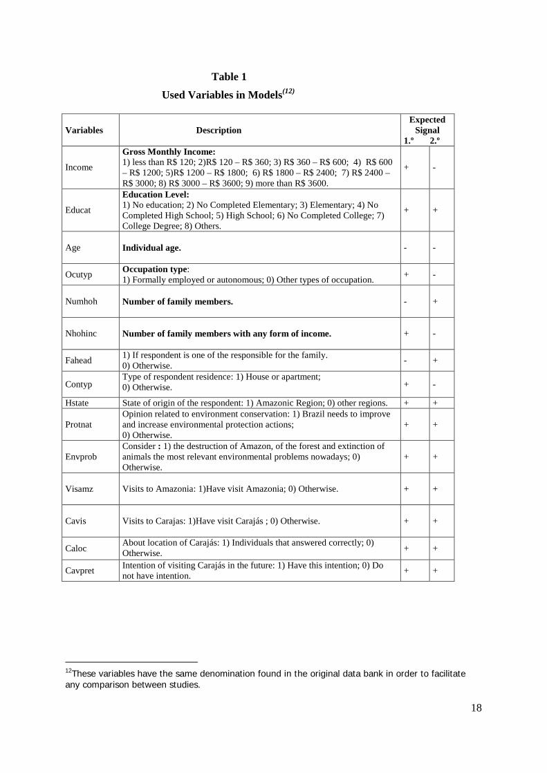
variables are described in Table 1, with its expected signal for each stage model.
RESULTS
Table 2 has as dependent variable the willingness to pay for environmental goods in the
Carajás region (WTPCA) and marginal effects of explanatory variables determine the
probability that variation of one unit of its measure, taking all other variables in their average,
10To construct a dependent variable to stage 2, those who answer that are unable to contribute received (1) and all other respondents received (0).
17
garantees the existence of willingness to pay for environmental goods in that region11. Tables
3 has as dependent variable - DZEXPCA – the behaviour of those individuals that have no
enough income, but would be willing to protect the environment. The idea is to confirm the
importance of variable “education” for these individuals with environmental concern but
without enough income.
According to GUJARATI (1995) there have been many tentatives to obtain measures that
would garantee the adjustment quality of dichotomous variable measures. Thus, a log
likelihood to test if all model coefficients are equal to zero is na important statistics to analyse
the model. In the first stage, using a Probit model one may observe, for the complete model, a
log likelihood of - 343.7728 and a significance level of (.0000) that garantees that the
model is significant. It is interesting to observe that only variables cavpret, fahead, contyp,
educat, ocutyp, income and age were significant in this model. In order to illustrate the
marginal effect of each coefficient let us take the variable related to education - educat.
11Coefficients of Probit model do not express directly marginal effects as in the case of usual regression models. In order to inffer about marginal effects of each variable in the model it is necessary to transform all other variables into their average. These variables have to be transformed into their average because the probability curve is not linear and, therefore, the position of each variable will influence the observed probability. Consequently, marginal effects showed in tables 2 and 3 express the probability that the variation of each variable makes the dependent variable be equal to (1).
18
Table 1 Used Variables in Models(12)
Variables Description Expected
Signal 1.º 2.º
Income
Gross Monthly Income: 1) less than R$ 120; 2)R$ 120 – R$ 360; 3) R$ 360 – R$ 600; 4) R$ 600 – R$ 1200; 5)R$ 1200 – R$ 1800; 6) R$ 1800 – R$ 2400; 7) R$ 2400 – R$ 3000; 8) R$ 3000 – R$ 3600; 9) more than R$ 3600.
+ -
Educat
Education Level: 1) No education; 2) No Completed Elementary; 3) Elementary; 4) No Completed High School; 5) High School; 6) No Completed College; 7) College Degree; 8) Others.
+ +
Age Individual age.
- -
Ocutyp Occupation type: 1) Formally employed or autonomous; 0) Other types of occupation. + -
Numhoh Number of family members.
- +
Nhohinc Number of family members with any form of income.
+ -
Fahead 1) If respondent is one of the responsible for the family. 0) Otherwise. - +
Contyp Type of respondent residence: 1) House or apartment; 0) Otherwise. + -
Hstate State of origin of the respondent: 1) Amazonic Region; 0) other regions. + +
Protnat Opinion related to environment conservation: 1) Brazil needs to improve and increase environmental protection actions; 0) Otherwise.
+ +
Envprob Consider : 1) the destruction of Amazon, of the forest and extinction of animals the most relevant environmental problems nowadays; 0) Otherwise.
+ +
Visamz Visits to Amazonia: 1)Have visit Amazonia; 0) Otherwise.
+ +
Cavis Visits to Carajas: 1)Have visit Carajás ; 0) Otherwise.
+ +
Caloc About location of Carajás: 1) Individuals that answered correctly; 0) Otherwise. + +
Cavpret Intention of visiting Carajás in the future: 1) Have this intention; 0) Do not have intention. + +
12These variables have the same denomination found in the original data bank in order to facilitate any comparison between studies.

19
Table 2
Stage 1 - Marginal Effects of Probit Model
Dependent Variable WTPCA
COMPLETE MODEL LIMITED MODEL
Log Likelihood - -348.8006 Chi – squared - 101.6418 Degrees of Freedom - 6 Significance level .00000000 Observations 673 Variables Marginal Effect Constant -.114906077 (-1.580) Cavpret .0663840047* (1.811) Fahead -.1317248092*** (-2.868) Contyp .1156177671*** (2.594) Educat .0288221827** (2.240) Income .0493514760*** (3.586) Age -.0077419355*** (-4.415)
Log Likelihood - -343.728 Chi – squared - 106.1167 Degrees of Freedom - 15 Significance level .00000000 Observations 673 Variables Marginal Effect Constant -.134578784 (-1.335) Pronat .433945237 (1.196) Hstate .031081708 (.212) Envprob .019992387 (.571) Visamz .062728227 (.969) Cavisit .181234662 (1.475) Caloc -.035079792 (-.855) Cavpret .06573602* (1.751) Nunhoh -.007635713 (-.711) Nhohinc .011323944 (.603) Fahead -.125023765** (-2.567) Contyp .107835268** (2.389) Educat .0292194655** (2.200) Ocutyp -.0111812612 (-.295) Income .0499655170*** (3.326) Age -.0783689395*** (-4.309)
Note: Significance Levels: ***1%, **5%, *10%.

20
Table 3
Stage 2 - Marginal Effects of Probit Model
Dependent Variable DZEXPCA
COMPLETE MODEL LIMITED MODEL Log Likelihood - -266.6729 Chi – squared - 65.16558 Degrees of Freedom - 15 Significance level .00000000 Observations 673 Variables Marginal Effect Constant .992991954 (.726) Pronat .0841980428* (1.829) Hstate -.0392845610 (-.172) Envprob .0448070654 (.981) Visamz .0259016230 (.262) Cavisit .1823996545 (1.108) Caloc -.0347683557 (-.610) Cavpret -.13563361*** (-2.867) Nunhoh -.003009434 (-.226) Nhohinc -.018051224 (-.716) Fahead .13928017* (1.885) Educat13 .030028480* (1.651) Ocutyp -.13577189*** (-2.658) Income -.04740737** (-2.120) Age -.005174695** (-2.514) Note: Significance Levels: ***1%, **5%, *10%.
Log Likelihood - -288.5607 Chi – squared - 22.21287 Degrees of Freedom - 3 Significance level .000058904 Observations 673 Variables Marginal Effect Constant .029997065 (.352) Educat .031478605* (2.240) Income -.074523908*** (-3.817) Age -.002847998 (-1.516)
13Variable Contyp presents a high correlation with variable Educat. We exclude it from complete models with dependent variable DZEXPCA.

21
For this model, the marginal coefficient for education (educat) was, aproximatelly, (0.29).
This means that the probability that an increase in one unit in the variable education will
increase in 2.9% the chance that the individual presents a WTP to avoid new large scale
projects in Carajás. Putting in a different way, a change in individual education from a level
of “non education” to a level of öne year of elementary school”, keeping constant all other
variables in their average, increases in 2.9% the chance of this individual to have a positive
WTP. This is a significant result, given that there are only eight intervals for the variable
education in our model, allowing for a very relevant influence in the determination of the
WTP for these environmental goods and services.
Furthermore, if we take the marginal effect for the main explanatory variable in the model –
income – we observe that an increase of one unit increases in 5% the chance of a positive
WTP, keeping other variables in their average. Once more, considering that there are nine
intervals for the variable income, one may notice that its effects are very significant upon the
dependent variable.
As far as signs of coefficients are concerned, it was observed that they are those expected for
all significative variables, with exception of Cavpret in the table 3. Nevertheless, results
confirm the importance of some socio-economic variables in the determination of WTP for
environmental goods and services related to Carajás. It can also be observed that by the log
likelihood the models were accepted. Finally, the importance of the limted model is to
demonstrate that similar results can be achieved with a simpler model. Analyses of marginal
effects of this second model can be in a similar fashion as the one done for the first model.
Results in Table 3 are those for models in the second stage of our econometric exercise. These
models, as mentioned before, have as dependent variable the behaviour of those individuals
who have an environmental demand, but do not have financial resources to pay for it. Both
models are significant and analyses of their marginal effects must be done in a similar fashion
to that of previous models. It is important to point out that variable education was significant
at the 10% level. This empirical evidence suggests that environmental consciousness may
grow as individual has more years of formal education. Literacy appears to be parfticularly
strong predictor of environmental externalities.

22
• Concluding Remarks
Econometric results achieved through these two stages and eight models allow us to test our
hypotheses in this study. First, it is clear the importance of socio-economic variables, in
particular income and education, in the determination of willingness to pay for environmental
goods and services. Second, the variable education is determinant in the behaviour of those
individuals who present an environmental demand, but are unable to materialise it due to lack
of financial resources. This suggests that an increment of individual wellfare, particularly in
education, will have a positive effect upon demand for environmental quality. It seems that
Grossman and Krueger (1995) and Boyce and Torras (2002) are correct in believing that
citizens’demand and “vigilance and advocacy” are critical in inducing policies and
technological changes with reduce degradation and pollution.
The main objective of this study was to provide evidence on how the Brazilian poverty –
manifested on a high concentration of income and a low level of education – might have
affect environmental demand and, therefore, the Environmental Kuznets Curve (EKC) in
Brazil. Having deforestation as indicator of environmental degradation we showed variables
influencing demand for environmental goods and services. A reduction in deforestation rate
means that individuals are prefering to conserve environmental assets instead of finding
alternative uses for them. Our resuilts also indicate that Brazilian poverty do affect demand
for environmental conservation in the Carajás region. Income concentration and difficulties in
the access to education affect deforestation rates in Brazil, at least indirectly through their
effects upon willingness to pay for conservation.
Some questions must be discussed after our findings. Some international institutions have
identified poverty as the cause of environmental degradation. They also suggest that economic
growth would be the basic solution for this problem. It seems from our study results, that
reduction in poverty level should deserve, at least, equivalent attention. Reduction of social
problems through increasing access to basic services by the poorest section of the population
shall increase significantly the demand for environmental goods and services. Economic
growth without distributive effects will not have similar impacts upon environmental demand.
23
Improvement of income, education and other social capital assets can lead to the formation of
a “tunnel” in the Environmental Kuznets Curve, avoiding excessive growth of environmental
degradation before it starts declining. Reduction of social and environmental vulnerability
would garantee a more equitable pattern of economic growth. Equity – reduction of
degradation and of poverty – and efficiency must receive equivalent consideration in
allowing communities to achieve their goals through a process of effective sustainable
development.
• Bibliography
AMEMIYA, T. Qualitative Response Model: A Survey, Journal of Economic Literature, v.19, p.
481-536, 1981.
ANSUATEGI, A.; BARBIER, E. B. & PERRINGS, C. A. The Environmental Kuznets Curve, paper
presented at the USF Workshop: Economic Modelling of Sustainable Development: Between Theory
and Practice, Free University, Amsterdam, 1996.
ARROW, K. ; BOLIN, B. ; CONSTANZA, R. ; DASGUPTA, P. ; FOLKE, C. ; HOLLING, C.S. ;
JANSSON, B-O. ; LEVIN, S. ; MÄLER, K-G. ; PERRINGS, C. & PIMENTEL, D. Economic
Growth, Carrying Capacity, and the Environment, Science, v.268, p. 520-521. 1995.
BARBIER, E.B. Natural Capital and the Economics of Environment and Development, in: A. Jansson,
M, Hammer, C. Folke, and R. Constanza, eds., Investing in Natural Capital: The Ecological
Economics Approach to Susteinability, New York: Columbia University Press. 1994.
BATEMAN, I & TUNER, R. K. Valuation of the Environment, Methods and Thecnics: The
Contigent Valuation Method. in: TUNER, R. Terry, Sustainable Environmental Economics and
Management. Principles and Practice. London: Belhaven Press, 1992.
BECKERMAN, W. Economic Growth and the Environment: Whose Growth? Whose Environment?.
World Development, v.20, p. 481-496, 1992.
BOYCE, James K. Inequality as a cause of Environmental Degradation. Ecological Economics , v.11,
p. 169-178, 1994.

24
BOYCE, James K. and TORRAS, Mariano. “Rethinking the environmental Kuznets curve.” Chapter 5
in J.K. Boyce. The Political Economy of the Environment. (Cheltenham, UK e Northampton, MA:
Edward Elgar, 2002), pp. 47-66.
BROAD, R. The Poor and the Environment: Friends or Foes?, World Development, v.22, no. 6, p.
811-822, 1994.
BRUYN, S.M., Explaining the Environmental Kuznets Curve: Structural Change and International
Agreements in Reducing Sulphur Emissions, Environmental and Development Economics , v.2 ,
p.485-503, 1997.
CARSON, R.T. ; JEON, Y. & McCUBBIN, D.R. The Relationship Between Air Polution Emissions
and Income: US Data, Environment and Development Economics, v.2, p. 433-450, 1997.
CROPPER, M. & GRIFFITHS, C. The Interaction of Population Growth and Environment Quality,
American Economic Review, v.84, p. 250-254, 1994.
DALY, H. & COBB, J.B. For the Common Good, Beacon Press, Boston MA . 1994.
EKINS, P., C. FOLKE, & R. CONSTANZA. Trade, Environment and Development. Ecological
Economics, v.9, p. 1-12, 1994.
EKINS, P. The Kuznets Curve for the Environment and Economic Growth: Examining the Evidence.
Environment and Plannig, v.29, p. 805-830, 1997.
FOSTER, B.A. Optimal Capital Accumulation in a Polluted Environment . Southern Economic
Journal, v.39, p. 544-547, 1973.
FREEMAN III, A.M. The Benefits of Environmental Improvement: Theory and Practice. Baltimore,
Md: The Johns Hopkins University Press for Resources for the Future, 1979.
___________________. The Measurement of Environmental and Resource Values: Theory and
Methods , Washington DC: Resources for the Future, p. 1-92. 1993.

25
GREEN, J.R. ; MAS-COLELL, A. & WHINSTON, M.D. Microeconomic Theory. Oxford
University Press. 1995.
GROSSMAN, G.M. & A.B. KRUEGER. Environmental Impacts of a North American Free Trade
Agreement. National Bureau of Economic Research Working Paper 3914, NBER, Cambridge, MA,
1991.
____________________________________. Environmental Impacts of a North American Free
Trade Agreement, in: P. Garber, ed., The US-Mexico Free Trade Agreement , Cambridge, MA: MIT
Press. 1994.
_____________________________________. Economic Growth and the Environment. Quarter
Journal Economic, v. 110, p. 353-377, 1995.
GUJARATI, D. Basic Econometrics.3rd edition , Mcgrall-Hill, Londres, 1995.
HANEMANN, W.M. Willingness to Pay Willingness to Accept: How much can they differ?,
American Economic Review, June, p. 635-647, 1991.
HICKS, J. R. The Rehabilitation of Consumers` Surplus, Review of Economic Studies, feb.8, p. 108-
116, 1941.
HOLTZ-EAKIN, D. & SELDEN, T. M. Stokinh the Fires? Co2 Emissions and Economic Growth,
Journal of Public Economics , v. 57, p. 85 -101, 1995.
HORVATH, R.J. Energy Consumption and the Environmental Kuznets Curve Debate, Department
of Geography, University of Sydney, 1997.
JOHN, A. & PECCHENINO. An Overlapping Generations Model of Growth and the Environment.
Economic Journal. v.104, p.1393-1410. 1994.
JOHANSSON, P. Cost - Benefit Analysis for Environmental Changes. Environmental Policy - Cost
Effectiveness, Press Syndicate of the University of Cambridge, 1993.
LOPEZ, R. The Environment as a Factor of Production: the Effects of Economic Growth and Trade
Liberalization. Journal of Environmental Economics and Management, v.27, p. 163-184, 1994.
26
KOMEN, M. H. C. ; GERKING, S. & FOLMER, H. Income and Environmental R&D: Empirical
Evidence from OECD countries, Environment and Development Economics, v.2, p. 505-515, 1997.
MARTINE, G. ; CARVALHO, J. A. M. Impacts of Spatial Patterns of Development and Population
Redistribution on the Demographic Transition. Brasilia: ISPN (Documento de Trabalho no 29), 1993.
11 p.
MASLOW, A. Higher and Lower Needs, Journal of Psychology, v.25, p.24-25, 1948.
McCONNEL, K. E. Income and the Demand for Environmental Quality. Environment and
Development Economics, v.2, p.383-399. 1997.
McFADDEN, D. Conditional Logit Analysis of Qualitative Choice Behavior. In P.Zarembka (ed.),
Frontiers in Econometrics, Academic Press, New York, 1973.
MENDOÇA, A.F. The Use Of Contigent Valuation Method to Assess the Environmental Cost Of
Mining In Serra Dos Carajás: Brazilian Amazon Region: Tese de Doutorado, Colorado School of
Mines, 1998.
MITCHELL, R. & CARSON, R. Using Surveys to Value Public Goods: The Contigent Valuation
Method. Resources For the Future, Washington D.C. 1989.
MUNASINGHE, M. An Overview of Environmental Impacts of Macroeconimic and Sectoral Policies,
in: M. Munasinghe (ed.), Environmental Impacts of Macroeconimic and Sectoral Policies,
Washington DC: World Bank , p. 1-14. 1996.
__________________. Countrywide policies and Sustainable Development: are the Linkages
Perverse? In: The International Yearbook of Environmental and Resource Economics 1998/1999 -
A Survey of Current Issues, p. 33-88, 1998.
NOGUEIRA, M.P.S. A Comparative Study of Some Models which Involve Dichotomous Dependent
Variable - A Cross Section Analysis. Dissertação de Mestrado, Universidade de Kent, 1982, p.125.
PANAYOTOU, T. Empirical Tests and Policy Analysis of Environmental Degradation at Different
Stages of Economic Development, Technology and Employment Programme, International Labour
Office, Geneva. 1993.

27
_________________. Environmental Degradation at Different Stages of Economic Development, in:
Ahmed and J.ª Doeleman, eds., Beyond Rio: The Environmental Crisis and Sustainable Livelihoods
in the Third World, London: MacMillan. 1995.
POLLAK, R. A. & WALES, T.J. Demand System Specification and Estimation, Oxford University
Press, New York, 1992.
PORTER, R. The New Approach to Wilderness Preservation Through Benefit-Cost Analyis,
Journal of Environmental Economics and Management, p.383-399, 1982.
SARMIENTO, B. Tecnicas de Valoracion de los Impactos Medioambientales en el Contexto del
Análisis Costo Beneficio, Cuadernos de Economia y Finanzas, Madrid, Fedea. 1995.
SELDEN, T.M. & SONG, D. Environmental Quality and Development: is there a Kuznets Curve for
Air Polution?, Journal of Environmental Economics and Management, v.27, p. 147-162. 1994.
SHAFIK, N. & BANDYOPADHYAY, S. Economic Growth and Environmental Quality: Time
Series and Cross-country Evidence, Background Paper for the World Development Report 1992, The
World Bank, Washington DC. 1992.
SHAFIK, N. Economic Development and Environmental Quality: an Econometric Analysis, Oxford
Economic Papers, v.46, p. 757-773, 1994.
STERN, D.I., M.S.COMMOM, and E.B. BARBIER. Economic Growth and Environmental
Degradation: the Environmental Kuznets Curve and Sustainable development. World Development,
v.24, p. 1151-1160, 1996.
STERN, D. I. Progress on the Environment Kuznets Curve? Environment and Development
Economics, v.3, p. 173-196. 1998.
SURI, V. AND D. CHAPMAN. Economic Growth, Trade and Energy: Implications for the
Environmental Kuznets Curve, Ecological Economics, special issue on EKC. 1997.
WORLD BANK . World Development Report 1992: Development and the Environment, Oxford
University Press, New York. 1992.
The ECO/UnB Working Paper Series
The Department of Economics of the University of Brasilia publishes its Working Papers Series since April 1972. On August 30, 2002 the series was renewed with the on-line publication of the papers. All Working Papers may be freely downloaded from the Department site: http://www.unb.br/ih/eco.
Working papers published since August 2002:
231 Posse de escravos e estrutura da riqueza no agreste e sertão de Pernambuco: 1777-1887. Flávio Rabelo Versiani and José Raimundo O. Vergolino, 30 August 2002, 29p.
232 On the natural rates of unemployment and interest: the Robertson connection. Mauro Boianovsky and John R. Presley, 30 August 2002, 34p.
233 Contas Nacionais e o meio ambiente: reflexões em torno de uma abordagem para o Brasil. Charles C. Mueller, 30 August 2002, 25p.
234 Economics of air pollution: hedonic price model and smell consequences of sewage treatment plants in urban areas. Sérgio A. Batalhone, Jorge M. Nogueira and Bernardo P. M. Mueller, 30 August 2002, 25p.
235 The Brazilian depression of the 80s and 90s. Mirta Bugarin, Roberto de G. Ellery Jr., Victor Gomes and Arilton Teixeira, 30 August 2002, 30p.
236 Informal employment in Brazil − A choice at the top and segmentation at the bottom: a quantile regression approach. Maria Tannuri-Pianto and Donald M. Pianto, 30 August 2002, 23p.
237 False contagion and false convergence clubs in stochastic growth theory. Stephen de Castro and Flávio Gonçalves, 30 August 2002, 20p.
238 Spot and contract markets in the Brazilian wholesale energy market. Paulo C. Coutinho and André Rossi de Oliveira, 30 August 2002, 19p.
239 Tributação da renda e do consumo no Brasil: uma abordagem macroeconômica. Valter Borges de Araújo Neto e Maria da C. S. de Sousa, 30 August 2002, 31p.
240 Vote splitting, reelection and electoral control: towards a unified model. Maurício S. Bugarin. 30 August 2002, 26p.
241 Shadow-prices in payment systems. Rodrigo Peñaloza, 6 September 2002, 31p.
242 Welfare implications of the Brazilian social security system. Roberto de G. Ellery Jr. and Mirta N. S. Bugarin, 13 September 2002, 28p.
243 Os agentes econômicos em processo de integração regional − Inferências para avaliar os efeitos da ALCA. Renato Baumann and Francisco Galrão Carneiro, 13 September 2002, 29p.
244 Leading by example: a simple evolutionary approach. André Rossi de Oliveira and João R. O. de Faria, 20 September 2002, 25p.
245 The role of institutions in sustainable development. Bernardo Mueller and Charles Mueller, 20 September 2002, 25p.
246 Incentivos em consórcios intermunicipais de saúde: uma abordagem de teoria dos contratos. Luciana Teixeira, Maria Cristina MacDowell and Mauricio Bugarin, 27 September 2002, 19p.
247 Liquidity constraints and the behavior of aggregate consumption over the Brazilian business cycle. Mirta Bugarin and Roberto de G. Ellery Jr, 27 September 2002, 19p.
248 Pricing water and sewage services in urban areas: Evidences of low level equilibrium in a developing economy. Ricardo Coelho de Faria, Jorge M. Nogueira and Bernardo

Mueller, 4 October 2002.
249 Wrong incentives for growth in the transition from modern slavery to labor markets: Babylon before, Babylon after. Stephen de Castro, 4 October 2002, 23p.
250 Vintage capital, distortions and development. Samuel Pessoa and Rafael Rob, 11 October 2002, 40p.
251 Consórcios intermunicipais de saúde: uma análise à luz da teoria dos jogos. Luciana Teixeira, Maria Cristina MacDowell and Mauricio Bugarin, 11 October 2002, 30p.
252 Preços de escravos em Pernambuco no século XIX. Flávio R. Versiani and José Raimundo O. Vergolino, 18 October 2002, 20p.
253 A model of capital accumulation and rent seeking. Paulo Barelli and Samuel de Abreu Pessoa, 18 October 2002, 47p.
254 Anchors away: the cost and benefits of Brazil’s devaluation. Edmund Amann and Werner Baer, 25 October 2002, 20p.
255 Um seguro agrícola “eficiente”. Aércio S. Cunha, 25 October 2002, 57p.
256 Campaign contributions with swing voters. Manfred Dix and Rudy Santore, 1 November 2002, 15p.
257 Incentivos para os administradores de empresas estatais: O papel dos dividendos mínimos obrigatórios e o desenho ótimo de salários. André Luís G. Carcia and Maurício Bugarin, 1 November 2002, 28p.
258 Impostos e a História. Aércio S. Cunha, 8 November 2002, 12p.
259 Determinantes do endividamento dos estados brasileiros: Uma análise de dados de painel. Isabela Fonte Boa Rosa Silva e Maria da Conceição Sampaio de Sousa, 8 November 2002, 27p.
260 Technology adoption: On the nonequivalence of tariffs and quotas. Arilton Teixeira, 15 November 2002, 25p.
261 Constitutional regimes, growth and stagnation in the Brazilian economy: 1947-1999. Marco Antônio Campos Martins, 15 November 2002, 39p.
262 Price caps and electoral cycles. César Mattos, 22 November 2002, 16p.
263 Os pobres que levantem a mão (mas será que são mesmo pobres?) - Uma tentativa de validar o cadastro único. Carlos Alberto Ramos and Ricardo Santana, 29 November 2002, 100p.
264 Relative earnings of immigrants and natives under changes in the US wage structure, 1970-1990: A quantile regression approach. Maria Tannuri-Pianto, 29 November 2002, 40p.
265 Bidding strategies in the Brazilian Treasury auctions. Anderson Caputo Silva, 6 December 2002, 34p.
266 Crises cambiais e ataques especulativos no Brasil. Mauro Costa Miranda, 13 December 2002, 26p.
267 Poverty and environment degradation: the Kuznets environmental curve for the Brazilian case. Fabio G. e Barros, Augusto F. Mendonça and Jorge M. Nogueira, 20 December 2002, 27p.
268 On shadow-prices of banks in real-time gross settlement systems. Rodrigo Peñaloza, 20 December 2002, 31 p.
269 A characterization of renegotiation-proof contracts via random fixed points in Banach

spaces. Rodrigo Peñaloza, 20 December 2002, 9 p.
Forthcoming working papers: (Subject to change)
270 Existence of time-invariant settlements in FEDWIRE-like payment systems. Rodrigo
Peñaloza, 27 December 2002, 13p.
271 Principal-Agent problem with continuum of constraints: the infinite dimensional approach. Rodrigo Peñaloza, 27 December 2002, 43p.
272 Structural analysis of multiple-unit auctions: recovering bidders’ valuations in auctions with dominant bidders. Anderson Caputo Silva, January 3, 2003, 18 p.
273 Financiamento público de campanhas eleitorais: efeitos sobre bem-estar social e representação partidária no Legislativo. Adriana C. Portugal and Maurício S. Bugarin, January 10, 2003, 25p.