Embed Size (px)
Citation preview
ACTeon
Potential impacts of desalination development on energy consumption DG Environment Study Contract #07037/2007/486641/EUT/D2
7 April 2008
ii
ACKNOWLEDGMENTS
This report would not have been possible without the help of Martina Flörke and her team from the University of Kassel, who provided us with relevant data from their WATERGAP model.
Under contract to: DG Research, European Commission Unit F4 – BU 5/ 03/06 Disclaimer: The views and statements expressed in this report are those of IEEP, Ecologic and ACTeon alone. Availability: This report is a deliverable to DG Environment of the European Commission and is not publicly available.
Authors: Jason Anderson, IEEP Samuela Bassi, IEEP Thomas Dworak, Ecologic Vienna Malcolm Fergusson, IEEP Cornelius Laaser, Ecologic Berlin Owen Le Mat, ACTeon Verena Matteiβ, ACTeon Pierre Strosser, ACTeon Keywords: Water scarcity, Desalination, Energy consumption Project Manager for IEEP: Jason Anderson, Senior Fellow Subcontractors to IEEP: Ecologic Vienna ACTeon
iii
Executive summary This study examines the growing problem of water scarcity in Europe, looking at anticipated conditions in 2030. It focuses on the option of meeting water deficits with desalination, and in particular what the energy use of desalination might be, the costs of energy and the associated CO2 emissions under several scenarios.
The Commission plans to launch an additional study in order to have an in-depth impact assessment of all alternative options. This means that the outcomes of the study focused on desalination and energy are not sufficient in themselves to address the opportunity of a further development of desalination across Europe. The outcomes of the study will have to be part of the expected more comprehensive overview of all options in terms of economic, social, environmental impacts.
Using the WaterGAP model under the LREM-E scenario, a list of river basins in Europe facing water deficits in 2030 is identified. This includes basins in 14 of the current 27 Member States, with a total water deficit of 80.75 km3 per year. A model is constructed of feasible desalination plant sites and water pumping routes to permit distribution in areas of scarcity.
The energy use to desalinate the water indicated as being in deficit is estimated in several ways. First, three scenarios are posed for the energy use of reverse osmosis desalination technology in 2030. The total annual energy requirement to meet the deficit ranges from approximately 194 TWh for the least efficiency technology assumption (2.4 kwh/m3 of water desalinated) to 67 TWh for the most efficient scenario (0.83 kwh/m3 – the theoretical minimum). In addition, the energy requirement to transport this water is estimated to be 98 TWh/ year.
A baseline energy use scenario is then drawn from a 2005 Primes model calculation in order to put these amounts in the perspective of total 2030 energy production for the countries in which these deficits are found. Under the worst case scenario energy requirements for desalination and transport are equivalent to 43% of Greece’s total energy production, 20% of Spain’s and 16% of Cyprus and Bulgaria’s energy production. Under more optimistic assumptions about desalination technology, these amounts fall by over 50%.
A second approach is taken to examine energy use, putting it in terms of overall EU-27 totals and no longer ascribing them just to the countries in which water deficits are found. Additionally, a new set of 2030 scenarios is introduced, including three where CO2 emissions levels are cut by 30% compared to 1990 levels. In these three scenarios, total energy use from desalination and transport ranges from an equivalent of 3 to 7% of total power production in 2030, with a commensurate proportion of CO2 emissions – ranging from 23 to 114 Mt annually. The cost of this power ranges between €8.5 billion and €15 billion per year. This translates to between 11 and 19 cents per cubic meter of water desalinated and transported to end users.
Given the recently proposed goals of cutting Europe’s greenhouse gas emissions by 20%, expanding renewable energy use to 20% and cutting energy use by 20%, desalination will be adding a large load at a time when cutting requirements is a growing priority. An examination of future scenarios finds that only one of the modelled scenarios, with a specific focus on energy efficiency and renewable energy, comes close to meeting the various goals.
Given the high cost of desalination, this study considers the possibility that it will put water beyond the feasible economic reach of consumers and hence may be limited by financial
iv
considerations in some areas. The metric used to examine this effect was to model desalination costs into future water prices and compare resulting prices with disposable household income. Taking 2% of total disposable income as a threshold of ‘disproportionate’ costs for water, only two river basins in Greece and two in Portugal just overstep this bound (at 2% and 2.1% respectively).
Finally, the potential for water saving to reduce energy requirements is explored. A range of options are discussed, and two savings scenarios are introduced to the energy models – whereby water demand is cut by 20% and 40%. These lead to energy demand cuts of 35% and 75% respectively. This means that water savings of 40% in combination with efficient desalination technology could lead to a case where the full water deficit could be desalinated using approximately 0.75% of Europe’s energy in 2030 – still not a negligible figure, but well below the 7% scenario with inefficient desalination and no water demand cuts.
The study concludes by considering a further benefit of water demand reduction – the knock-on effect of energy reduction in all of the uses to which water is put or subjected to, such as pumping, heating and treating. In three case studies (from Malta, Spain and the UK), the energy requirement aside from desalination is found to be around 10 kWh/m3 – energy that can be saved by cutting back on water needs.
v
Contents Executive summary iii
1 Introduction 7 1.1 Aim and general approach of this study 7 1.2 Clarification of terms 8
2 Estimating water stress in 2030 10 2.1 Introduction 10 2.2 The right scale for estimating water deficit 10 2.3 River basins facing water stress in 2030 10
3 Distribution of desalinated water 16 3.1 Starting point 16 3.2 End point 17 3.3 Transport route 17
4 Future energy use and CO2 emissions due to desalination 26 4.1 Energy use for desalination: methodology 26 4.1.1 Desalination as the central option: basic assumption 26 4.1.2 Background on technologies and energy use 26 4.1.3 Three energy use scenarios to be used in calculations 30 4.1.4 Energy to transport water 31 4.1.5 Estimating future CO2 Emissions and energy costs: based on the Primes
scenarios 31 4.2 Presentation of Results: energy use, CO2 emissions and energy costs in 2030 34 4.2.1 National energy use: baseline case in 2030 34 4.2.2 European energy, CO2 emissions, costs and future scenarios 36 4.3 Results in light of the Energy Policy for Europe 37
5 Financial feasibility of desalination 40 5.1 An indicator for measuring the financial feasibility 40 5.2 The method 41 5.2.1 Water prices 41 5.2.2 Desalination costs 42 5.2.3 Water consumption in households 44 5.2.4 Net disposable household income 44 5.3 Results 44
vi
5.4 Conclusion: high overall costs, but not at household level 47
6 The impact of water savings measures on energy use 48 6.1 The impact of water savings measures on desalination requirements 48 6.2 The impact of water savings measures on non-desalination energy
requirements: co-benefit case studies 53 6.2.1 Introduction 53 6.2.2 Energy consumption in the water cycle: basic features 53 6.2.3 Results from the three case studies 57 6.2.4 In summary 59
7 References 60
Annex A: Method to assess current water prices in river basins 61
Annex B: Method for estimating future “baseline” water prices 63 Urban Wastewater Treatment Directive 63 Drinking Water Directive (DWD) 66 Water Framework Directive - Cost-recovery 67
Annex C: Household water consumptions 69
Annex D: Method for assessing households net disposable incomes 71
Annex E: Current water prices in river basins 73
Annex F: Estimated future “baseline” water prices 79
Annex G: Data sources for energy consumption for different components of the water cycle 82
7
1 Introduction In recent years, a growing concern has been expressed throughout the European Union regarding drought events and water scarcity. For an increasing number of EU Member States, not limited anymore to Southern Europe as was traditionally the case, the occurrence of seasonal or longer term droughts and water scarcity situations have become a noticeable reality in recent years.
Among the options to cope with a lack of water suitable for domestic consumption, as well as irrigation and industrial use, is desalination. Already of crucial importance to the water supply in Middle Eastern countries, desalination is increasingly used in the drier parts of Europe, Australia, North America and elsewhere. With increasing pressures due to population growth, climate change, tourism and rising standards of living, even places traditionally free of water concerns will increasingly consider desalination as an option.
1.1 Aim and general approach of this study The objectives of this study are to assess the consequences of a scenario in which water scarcity in 2030 in Europe is compensated for by desalination. The impacts are calculated with respect to energy use, energy costs, desalination costs in the context of overall water pricing, and compatibility with the European climate and energy policy.
Note that it is not the mandate or goal of this study to consider all options to meet water requirements and compare their feasibility. It is explicitly the contracted mandate of this study to consider the role of desalination as the sole means of meeting water deficits. The Commission plans to launch an additional study in order to have an in-depth impact assessment of all alternative options. This means that the outcomes of the study focused on desalination and energy are not sufficient in themselves to address the opportunity of a further development of desalination across Europe. The outcomes of the study will have to be part of the expected more comprehensive overview of all options in terms of economic, social, environmental impacts.
In the present study, some consideration is given to the feasibility of desalination, as well as the effectiveness of water savings measures to reduce desalination and energy requirements, for illustrative purposes.
This study proceeds in the following steps:
• A scenario of future (2030) water scarcity (chapter 2)
- Identification of River basins with water stress in 2030;
- Identification of River Basins with a desalination option;
- Calculation of water deficits (to be made up for by desalination);
• Calculation of water transport distances (chapter 3)
• Energy use and CO2 emissions estimates (chapter 4)
- Calculate the energy needed to desalinate and transport the identified deficit, under three different technology scenarios;
8
- Estimate the associated CO2 produced based on three future energy supply scenarios;
- Estimate energy costs associated with those scenarios;
- Note energy supply implications, and the compatibility with the goals of the Energy Policy for Europe;
• The financial feasibility of desalination (chapter 5)
• The impact of water savings measures on energy use (chapter 6)
- Reduced energy due to desalination reduction;
- Reduced energy for other water-using processes;
- Three case studies
1.2 Clarification of terms In order to set up an appropriate definition for the purpose of the study, some terms have to be clarified:
• Water demand/use means the total volume of water needed to satisfy the different water services1, including volumes ‘lost’ during transport, for example leaks from pipes and evaporation.
• Water supply satisfies the water demand by providing water from various sources. This can be by withdrawals from natural hydrological regime in the river basin (surface and groundwater abstraction), rain water harvesting, water imports from other river basins and non-conventional production of water. Non-conventional sources of water include: (i) The production of freshwater by desalination of brackish water or saltwater; and (ii) The reuse of urban or industrial waste waters (with or without treatment), which increases the overall efficiency of use of water (extracted from primary sources). They are accounted for separately from natural renewable water resources2.
• Water consumption can be defined as Water abstracted which is no longer available for use because it has evaporated, transpired, been incorporated into products and crops, consumed by man or livestock, ejected directly into sea, or otherwise removed from freshwater resources. Water losses during transport of water between the points or points of abstractions and point or points of use are excluded.3.
• Water exploitation index: From all water that comes available by precipitation human beings abstract various amounts for different uses, usually grouped as domestic, agricultural, industrial, and energy use. The amount of water abstracted can be expressed as the percentage of total renewable water
1 In this study water service refers to water supply and waste water removal.
2 http://www.fao.org/ag/agl/aglw/aquastat/water_res/indexglos.htm.
3 http://glossary.eea.europa.eu/EEAGlossary/W/water_consumption.
9
resources. This is often referred to as the water exploitation index (Vallée & Margat 2003).
• Water stress occurs when the demand for water exceeds the available amount during a certain period or when poor quality restricts its use. It frequently occurs in areas with low rainfall and high population density or in areas where agricultural or industrial activities are intense. The EEA uses the following threshold values/ranges for the water exploitation index to indicate levels of water stress: (a) non-stressed countries < 10%; (b) low stress 10 to < 20%; (c) stressed 20% to < 40%; and (d) severe water stress ≥ 40%. The threshold values/ranges above are averages and it would be expected that areas for which the water exploitation index is above 20% would also be expected to experience severe water stress during drought or low river-flow periods4.
4 See EEA (2004): Indicator Fact Sheet (WQ1) Water exploitation index, available at
http://themes.eea.europa.eu/Specific_media/water/indicators/WQ01c%2C2004.05/WQ1_WaterExploitationIndex_130504.pdf
10
2 Estimating water stress in 2030
2.1 Introduction An initial task of this project is to estimate the water deficit in European river basins by 2030. Water deficit in the context of this study is regarded as is the quantity of water that exceeds a certain water exploitation level. For several reasons, estimating the water deficit in a river basin is a difficult task. The main drawback is insufficient data availability. Information on natural water availability and water abstraction is very patchy at river basin scale and depends strongly on the national framework and the structure of administration. Another challenge is to identify the points where the desalinated water shall be delivered to and to measure the distance to from the desalination plant. This information will feed the cost calculation of water transport as part of the overall cost calculation of desalination.
The aim of the section is to estimate the water deficit in European river basins under water stress in 2030. It will elucidate the approach chosen to calculate the water deficit and point out limitations and uncertainties. Furthermore, the distance from the desalination plant to the point of use is measured and the method presented.
2.2 The right scale for estimating water deficit The river basin can be seen as the unit that forms a complete and more or less independent hydrological cycle together with the sea and the atmosphere. From all water that comes available by precipitation human beings abstract various amounts for different uses, usually grouped as domestic, agricultural, industrial, and energy use. The amount of water abstracted can be expressed as the percentage of total renewable water resources. This is often referred to as the water exploitation index (Vallée & Margat 2003). More precise the water exploitation index (WEI) in a country is the mean annual total demand for freshwater divided by the long-term average freshwater resources. Water stress is usually defined to occur at a water exploitation index of 20%, severe water stress commencing from 40% (European Environment Agency, 2005). In this report the 20% threshold value is used.
For this report, the level of river basin districts was determined as the appropriate level. The river basin district was chosen as a compromise between the national scale on the one side which is too coarse and groups too many very different natural regions and, on the other side, hydrological river basins at smaller scales which may reveal reasons for local and regional water stress more accurately. However, it should be kept in mind that a river basin district can cover a large area of for example 63 200 km2 in the case of the Guadalquivir basin (Spanish part). It then combines a large number of sub basins at various sub scales and may cluster very different pressures on renewable water resources.
2.3 River basins facing water stress in 2030 The European Commission’s latest report on water scarcity and droughts (2007) identified river basins in Europe that currently suffer from water stress. This picture will be different in the year 2030 due to changes in water use and the effects of climate change on natural availability of water resources. The impacts of climate change will be highly pronounced by the
11
end of this century. However, uncertainty increases by order of magnitude, the farther in the future scenarios look. For this reason the time horizon of 2030 was chosen for this study. Uncertainty of model outputs are acceptable and at the same time signals of climate change can already be expected. Impacts of climate change will overlap with socio-economic developments. Advancements in technology and improved management of resources will lead to a drop of abstractions especially in the domestic, energy and agriculture sector by 2030. On the other side, demographic developments, water intensive life style and agricultural decisions (extent of irrigated area, choice of crop) may lead to local increase in water demand5.
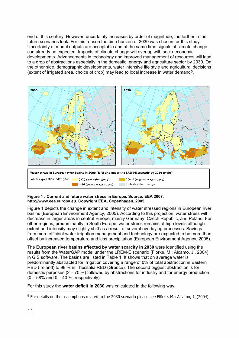
Figure 1 : Current and future water stress in Europe. Source: EEA 2007, http://www.eea.europa.eu. Copyright EEA, Copenhagen, 2005.
Figure 1 depicts the change in extent and intensity of water stressed regions in European river basins (European Environment Agency, 2005). According to this projection, water stress will decrease in larger areas in central Europe, mainly Germany, Czech Republic, and Poland. For other regions, predominantly in South Europe, water stress remains at high levels although extent and intensity may slightly shift as a result of several overlaying processes. Savings from more efficient water irrigation management and technology are expected to be more than offset by increased temperature and less precipitation (European Environment Agency, 2005).
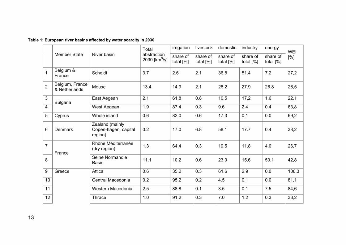
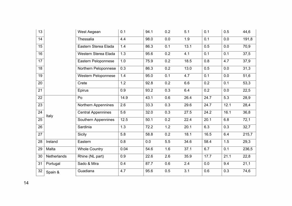
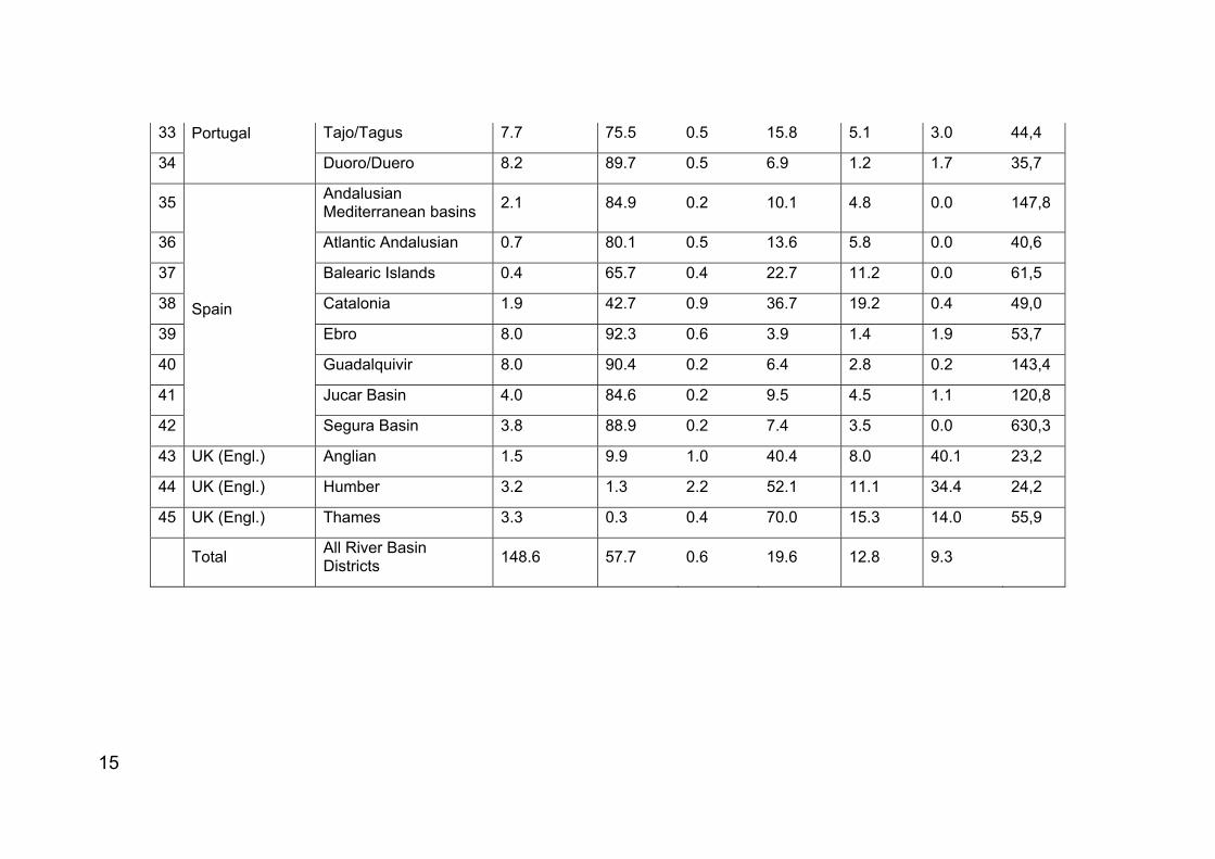
The European river basins affected by water scarcity in 2030 were identified using the results from the WaterGAP model under the LREM-E scenario (Flörke, M.; Alcamo, J., 2004) in GIS software. The basins are listed in Table 1. It shows that on average water is predominantly abstracted for irrigation covering a range of 0% of total abstraction in Eastern RBD (Ireland) to 98 % in Thessalia RBD (Greece). The second biggest abstraction is for domestic purposes (2 – 70 %) followed by abstractions for industry and for energy production (0 – 58% and 0 – 40 %, respectively).
For this study the water deficit in 2030 was calculated in the following way: 5 For details on the assumptions related to the 2030 scenario please see Flörke, M.; Alcamo, J.,(2004)
12
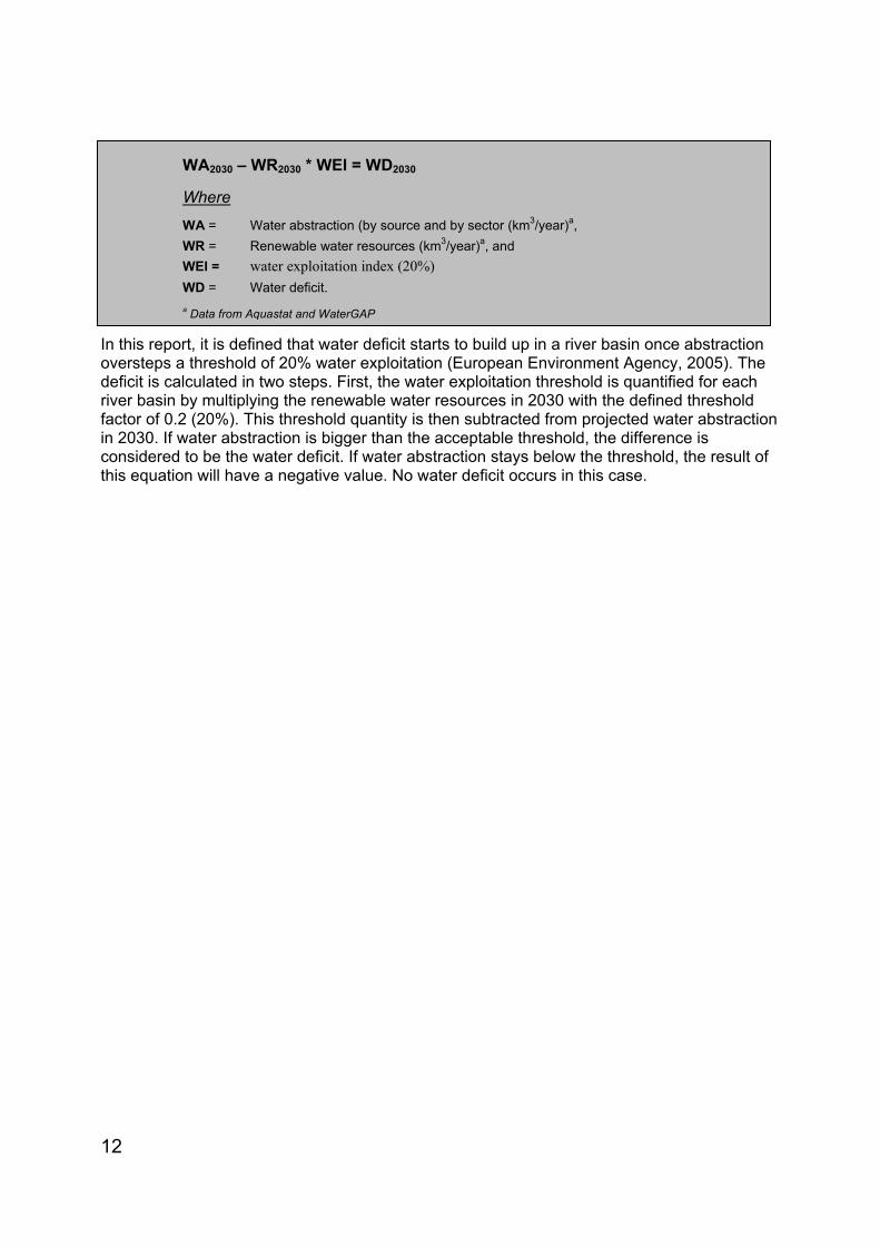
In this report, it is defined that water deficit starts to build up in a river basin once abstraction oversteps a threshold of 20% water exploitation (European Environment Agency, 2005). The deficit is calculated in two steps. First, the water exploitation threshold is quantified for each river basin by multiplying the renewable water resources in 2030 with the defined threshold factor of 0.2 (20%). This threshold quantity is then subtracted from projected water abstraction in 2030. If water abstraction is bigger than the acceptable threshold, the difference is considered to be the water deficit. If water abstraction stays below the threshold, the result of this equation will have a negative value. No water deficit occurs in this case.
WA2030 – WR2030 * WEI = WD2030
Where
WA = Water abstraction (by source and by sector (km3/year)a, WR = Renewable water resources (km3/year)a, and WEI = water exploitation index (20%) WD = Water deficit. a Data from Aquastat and WaterGAP
13
Table 1: European river basins affected by water scarcity in 2030
irrigation livestock domestic industry energy
Member State River basin Total abstraction 2030 [km3/y]
share of total [%]
share of total [%]
share of total [%]
share of total [%]
share of total [%]
WEI [%]
1 Belgium & France Scheldt 3.7 2.6 2.1 36.8 51.4 7.2 27,2
2 Belgium, France & Netherlands Meuse 13.4 14.9 2.1 28.2 27.9 26.8 26,5
3 East Aegean 2.1 61.8 0.8 10.5 17.2 1.6 22,1
4 Bulgaria
West Aegean 1.9 87.4 0.3 9.6 2.4 0.4 63,8
5 Cyprus Whole island 0.6 82.0 0.6 17.3 0.1 0.0 69,2
6 Denmark Zealand (mainly Copen-hagen, capital region)
0.2 17.0 6.8 58.1 17.7 0.4 38,2
7 Rhône Méditerranée (dry region) 1.3 64.4 0.3 19.5 11.8 4.0 26,7
8 France
Seine Normandie Basin 11.1 10.2 0.6 23.0 15.6 50.1 42,8
9 Attica 0.6 35.2 0.3 61.6 2.9 0.0 108,3
10 Central Macedonia 0.2 95.2 0.2 4.5 0.1 0.0 81,1
11 Western Macedonia 2.5 88.8 0.1 3.5 0.1 7.5 84,6
12
Greece
Thrace 1.0 91.2 0.3 7.0 1.2 0.3 33,2
14
13 West Aegean 0.1 94.1 0.2 5.1 0.1 0.5 44,6
14 Thessalia 4.4 98.0 0.0 1.9 0.1 0.0 191,8
15 Eastern Sterea Elada 1.4 86.3 0.1 13.1 0.5 0.0 70,9
16 Western Sterea Elada 1.3 95.6 0.2 4.1 0.1 0.1 37,5
17 Eastern Peloponnese 1.0 75.9 0.2 18.5 0.8 4.7 37,9
18 Northern Peloponnese 0.3 86.3 0.2 13.0 0.5 0.0 31,3
19 Western Peloponnese 1.4 95.0 0.1 4.7 0.1 0.0 51,6
20 Crete 1.2 92.8 0.2 6.6 0.2 0.1 53,3
21 Epirus 0.9 93.2 0.3 6.4 0.2 0.0 22,5
22 Po 14.9 43.1 0.6 26.4 24.7 5.3 28,9
23 Northern Appennines 2.6 33.3 0.3 29.6 24.7 12.1 28,4
24 Central Appennines 5.6 32.0 0.3 27.5 24.2 16.1 36,8
25 Southern Appennines 12.5 50.1 0.2 22.4 20.1 6.8 72,1
26 Sardinia 1.3 72.2 1.2 20.1 6.3 0.3 32,7
27
Italy
Sicily 5.8 58.8 0.2 18.1 16.5 6.4 215,7
28 Ireland Eastern 0.8 0.0 5.5 34.6 58.4 1.5 29,3
29 Malta Whole Country 0.04 54.6 1.6 37.1 6.7 0.1 236,5
30 Netherlands Rhine (NL part) 0.9 22.6 2.6 35.9 17.7 21.1 22,8
31 Portugal Sado & Mira 0.4 87.7 0.6 2.4 0.0 9.4 21,1
32 Spain & Guadiana 4.7 95.6 0.5 3.1 0.6 0.3 74,6
15
33 Tajo/Tagus 7.7 75.5 0.5 15.8 5.1 3.0 44,4
34
Portugal
Duoro/Duero 8.2 89.7 0.5 6.9 1.2 1.7 35,7
35 Andalusian Mediterranean basins 2.1 84.9 0.2 10.1 4.8 0.0 147,8
36 Atlantic Andalusian 0.7 80.1 0.5 13.6 5.8 0.0 40,6
37 Balearic Islands 0.4 65.7 0.4 22.7 11.2 0.0 61,5
38 Catalonia 1.9 42.7 0.9 36.7 19.2 0.4 49,0
39 Ebro 8.0 92.3 0.6 3.9 1.4 1.9 53,7
40 Guadalquivir 8.0 90.4 0.2 6.4 2.8 0.2 143,4
41 Jucar Basin 4.0 84.6 0.2 9.5 4.5 1.1 120,8
42
Spain
Segura Basin 3.8 88.9 0.2 7.4 3.5 0.0 630,3
43 UK (Engl.) Anglian 1.5 9.9 1.0 40.4 8.0 40.1 23,2
44 UK (Engl.) Humber 3.2 1.3 2.2 52.1 11.1 34.4 24,2
45 UK (Engl.) Thames 3.3 0.3 0.4 70.0 15.3 14.0 55,9
Total All River Basin Districts 148.6 57.7 0.6 19.6 12.8 9.3
16
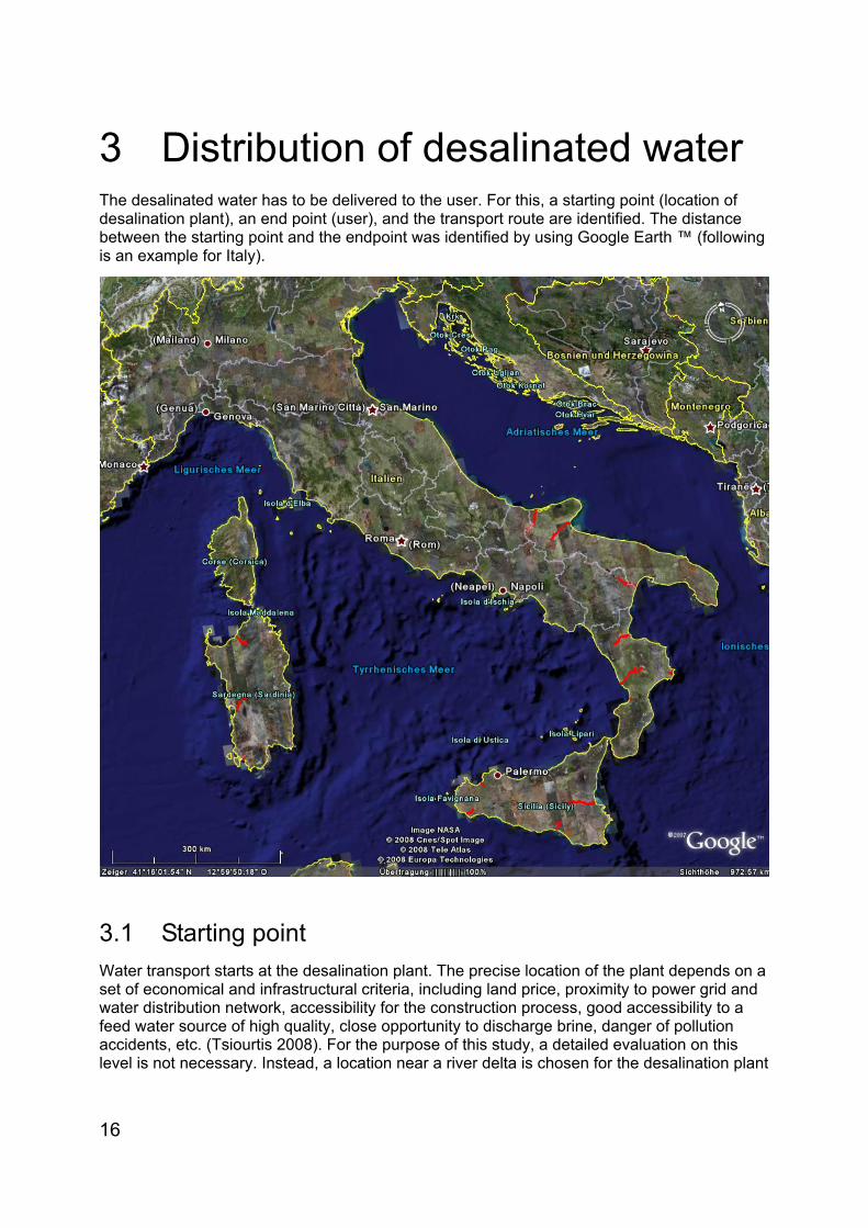
3 Distribution of desalinated water The desalinated water has to be delivered to the user. For this, a starting point (location of desalination plant), an end point (user), and the transport route are identified. The distance between the starting point and the endpoint was identified by using Google Earth ™ (following is an example for Italy).
3.1 Starting point Water transport starts at the desalination plant. The precise location of the plant depends on a set of economical and infrastructural criteria, including land price, proximity to power grid and water distribution network, accessibility for the construction process, good accessibility to a feed water source of high quality, close opportunity to discharge brine, danger of pollution accidents, etc. (Tsiourtis 2008). For the purpose of this study, a detailed evaluation on this level is not necessary. Instead, a location near a river delta is chosen for the desalination plant
17
in general, being close to the feed water source, the sink for discharging the brine, and the supposed transport route (section 3.3).
3.2 End point For the end point existing infrastructure was identified. Such infrastructure can be existing urban supply systems or reservoirs for agricultural irrigation.
In case additional water is needed for agriculture the end point lies in most cases some point upstream in the river basin where water is needed for irrigation. It is assumed to be most cost-effective to pump water in reservoirs upstream as they exist already in many water stressed countries and are used for irrigation. Moreover, from there an infrastructure for irrigation should be in place already. In the case where currently no reservoir exists as suitable place in the centre was identified. [do not understand this sentence]
In case additional water is needed for domestic, industrial and energy use, the end point is an access point to the regional or local water supply system. If the domestic area is located near the coast, a general average transport route of 5 km is assumed. For urban areas situated further inland, desalinated water will be transported to the nearest reservoir as well. In that case, reservoirs serve multipurpose uses (irrigation and domestic supply).
It should be noted that these are estimates to permit modelling and are not reflective of nor to be used for detailed planning.
3.3 Transport route It is assumed that the desalination plant is located close to the sea and close to the delta of the main river of the catchment. Further it is assumed that all pipelines are located next to the river, as this would require the least energy for pumping it upstream to a location in the river basin (natural water course follow the way of the lowest resistance). The route (pipeline) is therefore planned upstream more or less along the river course. Where a linear infrastructure such as a channel or a road is close to the river, this route was followed instead of the sinuous river course.
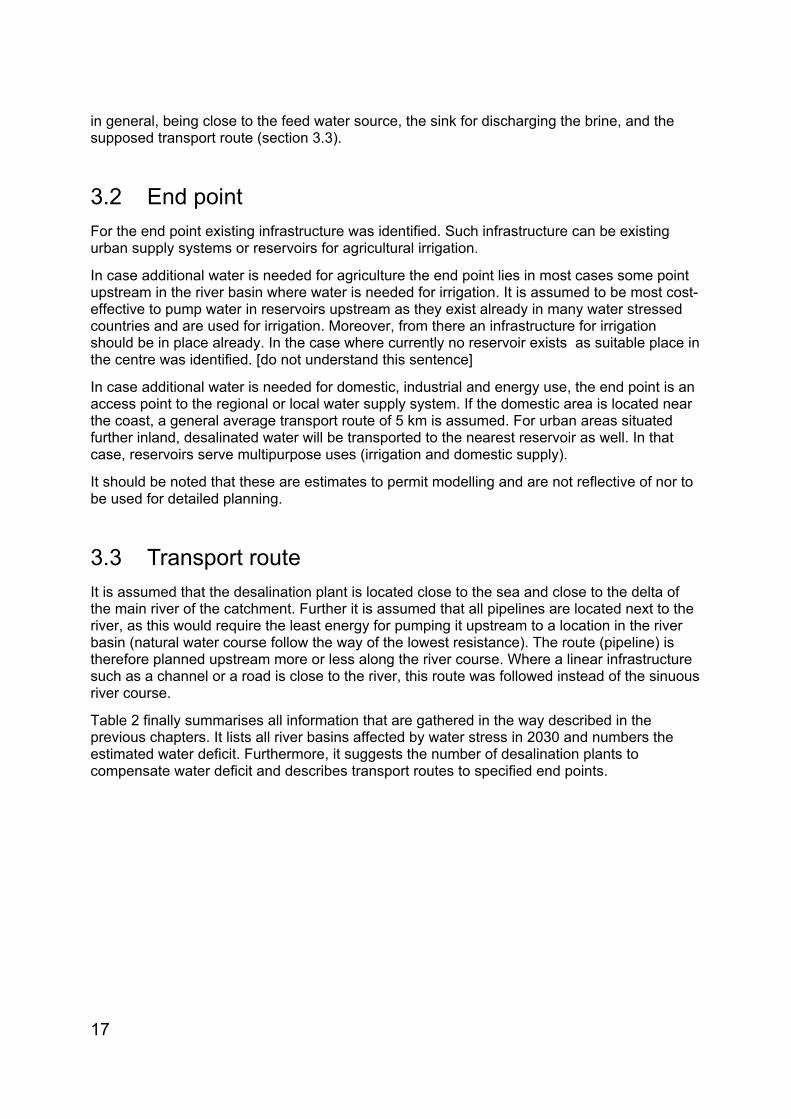
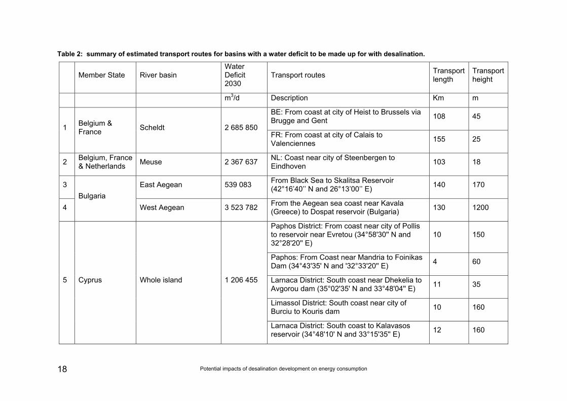
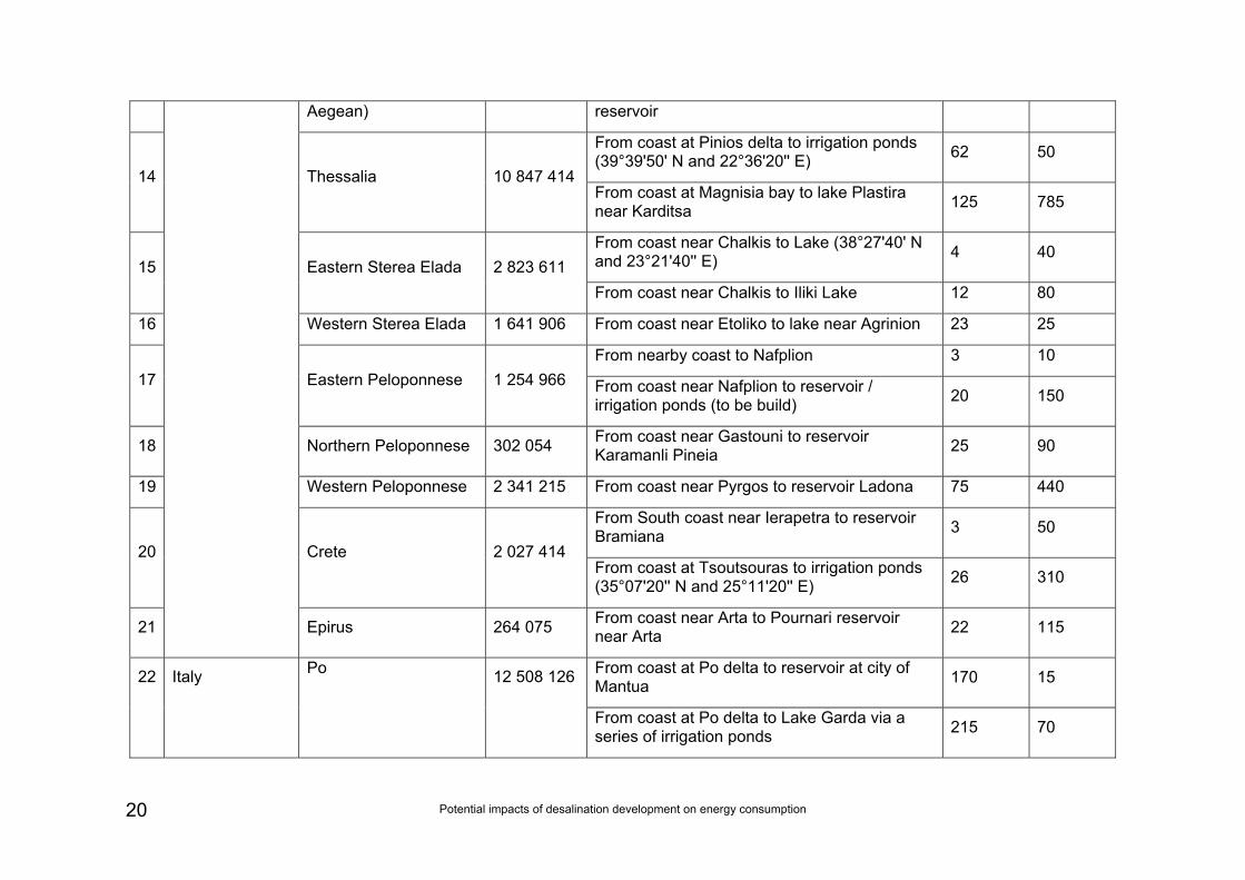
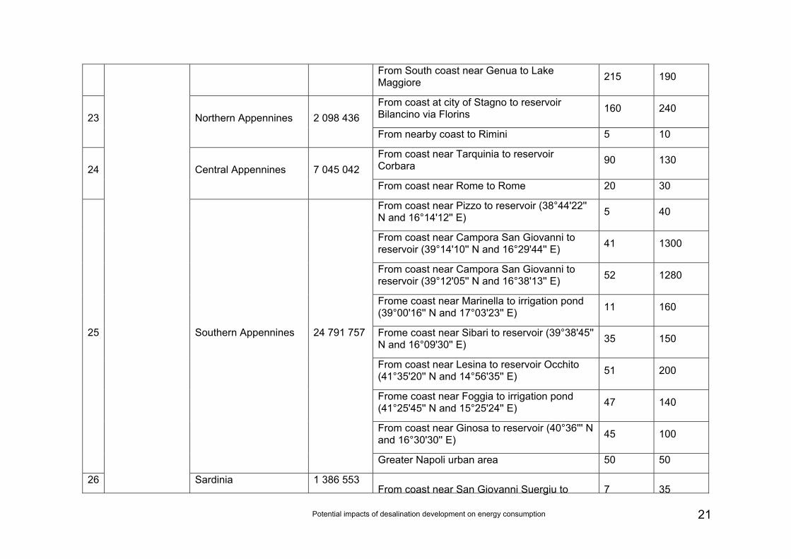
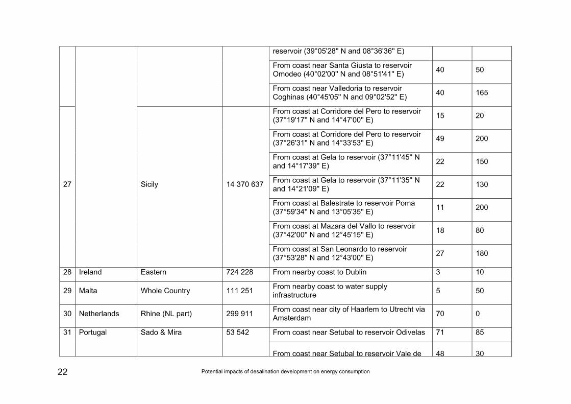
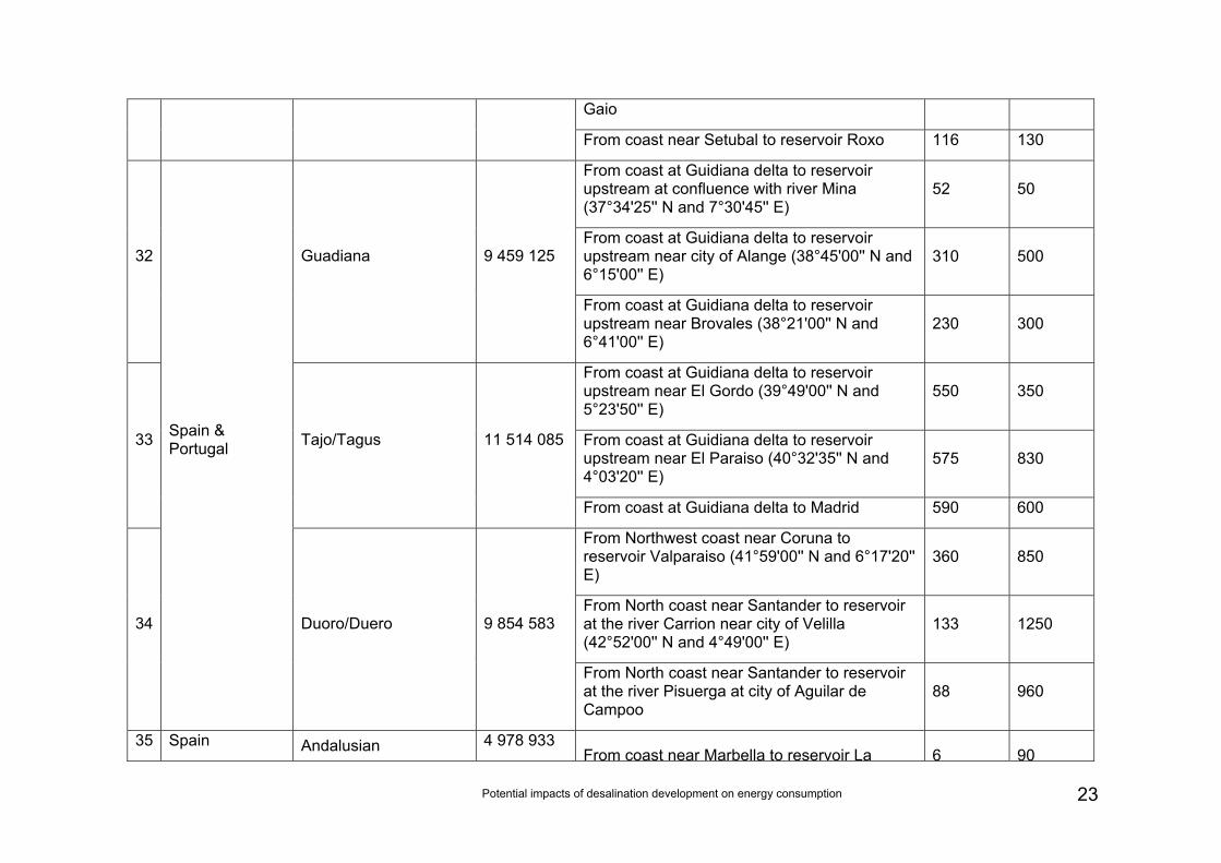
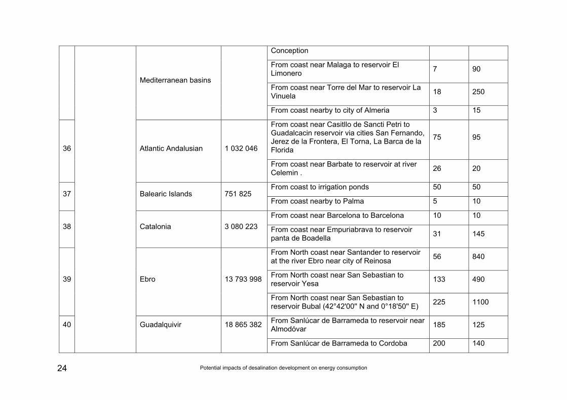
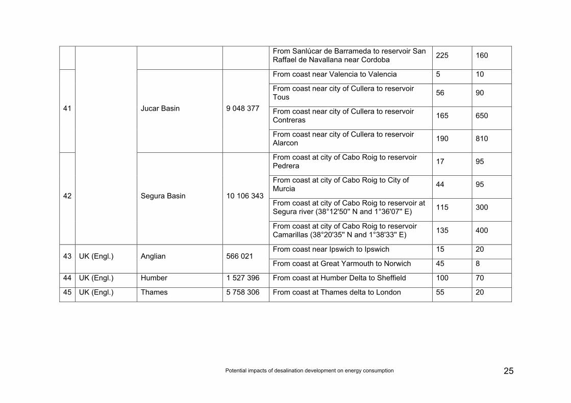
Table 2 finally summarises all information that are gathered in the way described in the previous chapters. It lists all river basins affected by water stress in 2030 and numbers the estimated water deficit. Furthermore, it suggests the number of desalination plants to compensate water deficit and describes transport routes to specified end points.
Potential impacts of desalination development on energy consumption 18
Table 2: summary of estimated transport routes for basins with a water deficit to be made up for with desalination.
Member State River basin Water Deficit 2030
Transport routes Transport length
Transport height
m3/d Description Km m
BE: From coast at city of Heist to Brussels via Brugge and Gent 108 45
1 Belgium & France Scheldt 2 685 850
FR: From coast at city of Calais to Valenciennes 155 25
2 Belgium, France & Netherlands Meuse 2 367 637 NL: Coast near city of Steenbergen to
Eindhoven 103 18
3 East Aegean 539 083 From Black Sea to Skalitsa Reservoir (42°16’40’’ N and 26°13’00’’ E) 140 170
4 Bulgaria
West Aegean 3 523 782 From the Aegean sea coast near Kavala (Greece) to Dospat reservoir (Bulgaria) 130 1200
Paphos District: From coast near city of Pollis to reservoir near Evretou (34°58'30'' N and 32°28'20'' E)
10 150
Paphos: From Coast near Mandria to Foinikas Dam (34°43'35' N and '32°33'20'' E) 4 60
Larnaca District: South coast near Dhekelia to Avgorou dam (35°02'35' N and 33°48'04'' E) 11 35
Limassol District: South coast near city of Burciu to Kouris dam 10 160
5 Cyprus Whole island 1 206 455
Larnaca District: South coast to Kalavasos reservoir (34°48'10' N and 33°15'35'' E) 12 160
Potential impacts of desalination development on energy consumption 19
6 Denmark Zealand (mainly Copen-hagen, capital region)
267 828 From nearby coast to Copenhagen supply infrastructure 3 10
From Saint-Laurent-de-la-Salanque to reservoir Caramany 42 170
From the coast at Canet-Plage to Reservoir Vinca via Perpignan 44 230 7 Rhône Méditerranée
(dry region) 878 431
From the coast at Agne to Reservoir Salagou 60 170
8
France
Seine Normandie Basin6 16 195 567 From coast near Le Havre to Paris 190 90
From coast near Marathon to reservoir Marathon 14 230
9 Attica 1 309 799 From coast nearby to Athens 5 20
10 Central Macedonia 481 301 From coast at mouth of river Axios upstream to small dam (40°45'08' N and 22°38'30'' E) 27 15
From coast at mouth of Aliakmonas river upstream to 2 reservoirs (first after 41 km, 30m)
68 280 11 Western Macedonia 5 290 227
From coast at mouth of Aliakmonas river upstream to Lake Vegoritis 100 515
12 Thrace (GR part of East Eagean) 1 126 142 From Nestos to Thisauros reservoir 85 250
13
Greece
Eastern Macedonia (GR part of West
134 091 From South coast near Lake Volvi to Kerkini 82 50 6 Most of the water deficit is coming from energy production. It has to be considered that there better options (e.g. new power plants with less water
consumption) to reduce the water deficit in this case. However as the study is based on the assumption that all water deficit is reduced by desalination these other options are not considered.
Potential impacts of desalination development on energy consumption 20
Aegean) reservoir
From coast at Pinios delta to irrigation ponds (39°39'50' N and 22°36'20'' E) 62 50
14 Thessalia 10 847 414 From coast at Magnisia bay to lake Plastira near Karditsa 125 785
From coast near Chalkis to Lake (38°27'40' N and 23°21'40'' E) 4 40
15 Eastern Sterea Elada 2 823 611 From coast near Chalkis to Iliki Lake 12 80
16 Western Sterea Elada 1 641 906 From coast near Etoliko to lake near Agrinion 23 25
From nearby coast to Nafplion 3 10 17 Eastern Peloponnese 1 254 966 From coast near Nafplion to reservoir /
irrigation ponds (to be build) 20 150
18 Northern Peloponnese 302 054 From coast near Gastouni to reservoir Karamanli Pineia 25 90
19 Western Peloponnese 2 341 215 From coast near Pyrgos to reservoir Ladona 75 440
From South coast near Ierapetra to reservoir Bramiana 3 50
20 Crete 2 027 414 From coast at Tsoutsouras to irrigation ponds (35°07'20'' N and 25°11'20'' E) 26 310
21 Epirus 264 075 From coast near Arta to Pournari reservoir near Arta 22 115
From coast at Po delta to reservoir at city of Mantua 170 15 22 Italy Po
12 508 126
From coast at Po delta to Lake Garda via a series of irrigation ponds 215 70
Potential impacts of desalination development on energy consumption 21
From South coast near Genua to Lake Maggiore 215 190
From coast at city of Stagno to reservoir Bilancino via Florins 160 240
23 Northern Appennines 2 098 436 From nearby coast to Rimini 5 10
From coast near Tarquinia to reservoir Corbara 90 130
24 Central Appennines 7 045 042 From coast near Rome to Rome 20 30
From coast near Pizzo to reservoir (38°44'22'' N and 16°14'12'' E) 5 40
From coast near Campora San Giovanni to reservoir (39°14'10'' N and 16°29'44'' E) 41 1300
From coast near Campora San Giovanni to reservoir (39°12'05'' N and 16°38'13'' E) 52 1280
Frome coast near Marinella to irrigation pond (39°00'16'' N and 17°03'23'' E) 11 160
Frome coast near Sibari to reservoir (39°38'45'' N and 16°09'30'' E) 35 150
From coast near Lesina to reservoir Occhito (41°35'20'' N and 14°56'35'' E) 51 200
Frome coast near Foggia to irrigation pond (41°25'45'' N and 15°25'24'' E) 47 140
From coast near Ginosa to reservoir (40°36''' N and 16°30'30'' E) 45 100
25 Southern Appennines 24 791 757
Greater Napoli urban area 50 50
26 Sardinia 1 386 553 From coast near San Giovanni Suergiu to 7 35
Potential impacts of desalination development on energy consumption 22
reservoir (39°05'28'' N and 08°36'36'' E)
From coast near Santa Giusta to reservoir Omodeo (40°02'00'' N and 08°51'41'' E) 40 50
From coast near Valledoria to reservoir Coghinas (40°45'05'' N and 09°02'52'' E) 40 165
From coast at Corridore del Pero to reservoir (37°19'17'' N and 14°47'00'' E) 15 20
From coast at Corridore del Pero to reservoir (37°26'31'' N and 14°33'53'' E) 49 200
From coast at Gela to reservoir (37°11'45'' N and 14°17'39'' E) 22 150
From coast at Gela to reservoir (37°11'35'' N and 14°21'09'' E) 22 130
From coast at Balestrate to reservoir Poma (37°59'34'' N and 13°05'35'' E) 11 200
From coast at Mazara del Vallo to reservoir (37°42'00'' N and 12°45'15'' E) 18 80
27 Sicily 14 370 637
From coast at San Leonardo to reservoir (37°53'28'' N and 12°43'00'' E) 27 180
28 Ireland Eastern 724 228 From nearby coast to Dublin 3 10
29 Malta Whole Country 111 251 From nearby coast to water supply infrastructure 5 50
30 Netherlands Rhine (NL part) 299 911 From coast near city of Haarlem to Utrecht via Amsterdam 70 0
From coast near Setubal to reservoir Odivelas 71 85 31 Portugal Sado & Mira 53 542
From coast near Setubal to reservoir Vale de 48 30
Potential impacts of desalination development on energy consumption 23
Gaio
From coast near Setubal to reservoir Roxo 116 130
From coast at Guidiana delta to reservoir upstream at confluence with river Mina (37°34'25'' N and 7°30'45'' E)
52 50
From coast at Guidiana delta to reservoir upstream near city of Alange (38°45'00'' N and 6°15'00'' E)
310 500 32 Guadiana 9 459 125
From coast at Guidiana delta to reservoir upstream near Brovales (38°21'00'' N and 6°41'00'' E)
230 300
From coast at Guidiana delta to reservoir upstream near El Gordo (39°49'00'' N and 5°23'50'' E)
550 350
From coast at Guidiana delta to reservoir upstream near El Paraiso (40°32'35'' N and 4°03'20'' E)
575 830 33 Tajo/Tagus 11 514 085
From coast at Guidiana delta to Madrid 590 600
From Northwest coast near Coruna to reservoir Valparaiso (41°59'00'' N and 6°17'20'' E)
360 850
From North coast near Santander to reservoir at the river Carrion near city of Velilla (42°52'00'' N and 4°49'00'' E)
133 1250 34
Spain & Portugal
Duoro/Duero 9 854 583
From North coast near Santander to reservoir at the river Pisuerga at city of Aguilar de Campoo
88 960
35 Spain Andalusian 4 978 933 From coast near Marbella to reservoir La 6 90
Potential impacts of desalination development on energy consumption 24
Conception
From coast near Malaga to reservoir El Limonero 7 90
From coast near Torre del Mar to reservoir La Vinuela 18 250
Mediterranean basins
From coast nearby to city of Almeria 3 15
From coast near Casitllo de Sancti Petri to Guadalcacin reservoir via cities San Fernando, Jerez de la Frontera, El Torna, La Barca de la Florida
75 95 36 Atlantic Andalusian 1 032 046
From coast near Barbate to reservoir at river Celemin . 26 20
From coast to irrigation ponds 50 50 37 Balearic Islands 751 825
From coast nearby to Palma 5 10
From coast near Barcelona to Barcelona 10 10 38 Catalonia 3 080 223 From coast near Empuriabrava to reservoir
panta de Boadella 31 145
From North coast near Santander to reservoir at the river Ebro near city of Reinosa 56 840
From North coast near San Sebastian to reservoir Yesa 133 490 39 Ebro 13 793 998
From North coast near San Sebastian to reservoir Bubal (42°42'00'' N and 0°18'50'' E) 225 1100
From Sanlúcar de Barrameda to reservoir near Almodóvar 185 125 40 Guadalquivir 18 865 382
From Sanlúcar de Barrameda to Cordoba 200 140
Potential impacts of desalination development on energy consumption 25
From Sanlúcar de Barrameda to reservoir San Raffael de Navallana near Cordoba 225 160
From coast near Valencia to Valencia 5 10
From coast near city of Cullera to reservoir Tous 56 90
From coast near city of Cullera to reservoir Contreras 165 650
41 Jucar Basin 9 048 377
From coast near city of Cullera to reservoir Alarcon 190 810
From coast at city of Cabo Roig to reservoir Pedrera 17 95
From coast at city of Cabo Roig to City of Murcia 44 95
From coast at city of Cabo Roig to reservoir at Segura river (38°12'50'' N and 1°36'07'' E) 115 300
42 Segura Basin 10 106 343
From coast at city of Cabo Roig to reservoir Camarillas (38°20'35'' N and 1°38'33'' E) 135 400
From coast near Ipswich to Ipswich 15 20 43 UK (Engl.) Anglian 566 021
From coast at Great Yarmouth to Norwich 45 8
44 UK (Engl.) Humber 1 527 396 From coast at Humber Delta to Sheffield 100 70
45 UK (Engl.) Thames 5 758 306 From coast at Thames delta to London 55 20
Potential impacts of desalination development on energy consumption 26
4 Future energy use and CO2 emissions due to desalination
4.1 Energy use for desalination: methodology
4.1.1 Desalination as the central option: basic assumption
Chapter 2 indicated the likely water deficit by river basin in Europe in 2030. The central assumption of this section is that these deficits will be made up for by use of desalination of seawater. Clearly there are a number of assumptions and approximations made in that central case – including notably that desalination would be the primary means of making up for the shortfall. The selection of the most appropriate mean among all existing options will be the subject of a next study to be launched by the Commission. This means that the outcomes of the study focused on desalination and energy are not sufficient in themselves to address the opportunity of a further development of desalination across Europe. The outcomes of the study will have to be part of the expected more comprehensive overview of all options in terms of economic, social, environmental impacts.
After a review of desalination technology we therefore pose a basic case in which energy use, associated CO2 emissions and energy costs are estimated. In chapter six we consider some alternative cases.
4.1.2 Background on technologies and energy use
The first desalination technologies were based on thermal processes. These produce the highest quality output water, but at very high energy costs. Hence, currently thermal desalination is being increasingly substituted by the (relatively) less energy demanding membrane processes - especially reverse osmosis. These are now widely used in the majority of the world's new and planned desalination plants. Nevertheless, thermal processes are still common in the Arabian Gulf states, and still account for 40% of worldwide distillation capacity.
Potential impacts of desalination development on energy consumption 27
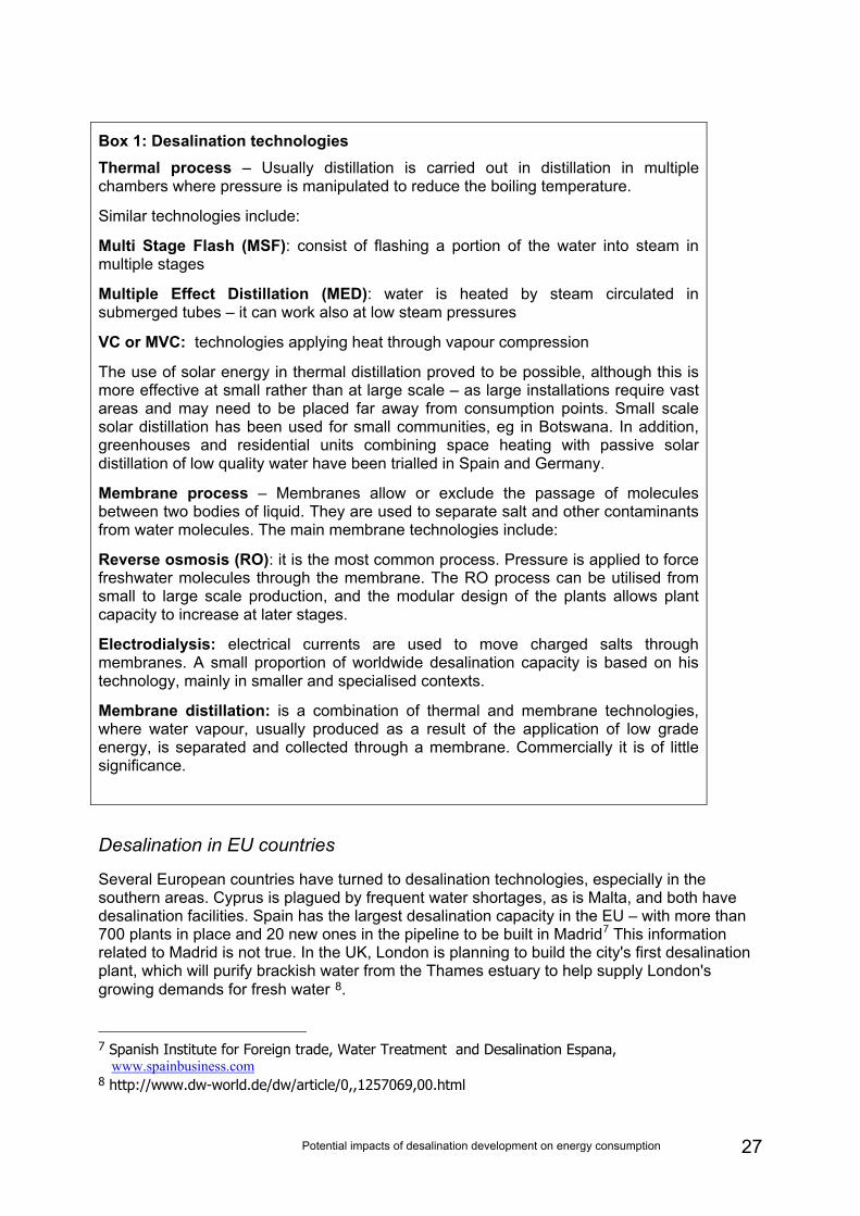
Box 1: Desalination technologies Thermal process – Usually distillation is carried out in distillation in multiple chambers where pressure is manipulated to reduce the boiling temperature.
Similar technologies include:
Multi Stage Flash (MSF): consist of flashing a portion of the water into steam in multiple stages
Multiple Effect Distillation (MED): water is heated by steam circulated in submerged tubes – it can work also at low steam pressures
VC or MVC: technologies applying heat through vapour compression
The use of solar energy in thermal distillation proved to be possible, although this is more effective at small rather than at large scale – as large installations require vast areas and may need to be placed far away from consumption points. Small scale solar distillation has been used for small communities, eg in Botswana. In addition, greenhouses and residential units combining space heating with passive solar distillation of low quality water have been trialled in Spain and Germany.
Membrane process – Membranes allow or exclude the passage of molecules between two bodies of liquid. They are used to separate salt and other contaminants from water molecules. The main membrane technologies include:
Reverse osmosis (RO): it is the most common process. Pressure is applied to force freshwater molecules through the membrane. The RO process can be utilised from small to large scale production, and the modular design of the plants allows plant capacity to increase at later stages.
Electrodialysis: electrical currents are used to move charged salts through membranes. A small proportion of worldwide desalination capacity is based on his technology, mainly in smaller and specialised contexts.
Membrane distillation: is a combination of thermal and membrane technologies, where water vapour, usually produced as a result of the application of low grade energy, is separated and collected through a membrane. Commercially it is of little significance.
Desalination in EU countries
Several European countries have turned to desalination technologies, especially in the southern areas. Cyprus is plagued by frequent water shortages, as is Malta, and both have desalination facilities. Spain has the largest desalination capacity in the EU – with more than 700 plants in place and 20 new ones in the pipeline to be built in Madrid7 This information related to Madrid is not true. In the UK, London is planning to build the city's first desalination plant, which will purify brackish water from the Thames estuary to help supply London's growing demands for fresh water 8.
7 Spanish Institute for Foreign trade, Water Treatment and Desalination Espana,
www.spainbusiness.com 8 http://www.dw-world.de/dw/article/0,,1257069,00.html
Potential impacts of desalination development on energy consumption 28
The energy consumption of desalination
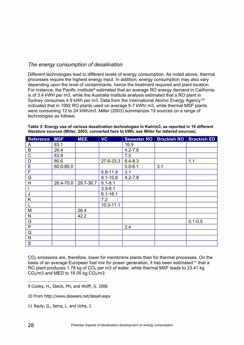
Different technologies lead to different levels of energy consumption. As noted above, thermal processes require the highest energy input. In addition, energy consumption may also vary depending upon the level of contaminants, hence the treatment required and plant location. For instance, the Pacific Institute9 estimated that an average RO energy demand in California is of 3.4 kWH per m3, while the Australia Institute analysis estimated that a RO plant in Sydney consumes 4.9 kWh per m3. Data from the International Atomic Energy Agency10 indicated that in 1992 RO plants used on average 5-7 kWh/ m3, while thermal MSF plants were consuming 12 to 24 kWh/m3. Miller (2003) summarizes 19 sources on a range of technologies as follows:
Table 3: Energy use of various desalination technologies in Kwh/m3, as reported in 19 different literature sources (Miller, 2003; converted here to kWh. see Miller for lettered sources).
Reference MSF MEE VC Seawater RO Brackish RO Brackish EDA 83.1 16.9 B 26.4 4.2-7.8 C 63.9 7.5 D 80.6 27.8-33.3 6.4-8.3 1.1 E 60.0-80.0 5.0-6.1 3.1 F 6.9-11.9 3.1 G 8.1-10.8 4.2-7.8 H 26.4-70.0 29.7-36.7 6.1-8.1 I 3.9-8.1 J 6.1-16.1 K 7.2 L 10.3-11.1 M 26.4 N 42.2 O 0.1-0.5 P 2.4 Q R S
CO2 emissions are, therefore, lower for membrane plants than for thermal processes. On the basis of an average European fuel mix for power generation, it has been estimated11 that a RO plant produces 1.78 kg of CO2 per m3 of water, while thermal MSF leads to 23.41 kg CO2/m3 and MED to 18.05 kg CO2/m3.
9 Cooley, H., Gleick, PH, and Wolff, G. 2006
10 From http://www.desware.net/desa4.aspx
11 Rauly, G., Serra, L. and Uche, J.

Potential impacts of desalination development on energy consumption 29
Potential impacts of desalination development on energy consumption 30
Box 2: High reliance on desalination in Malta
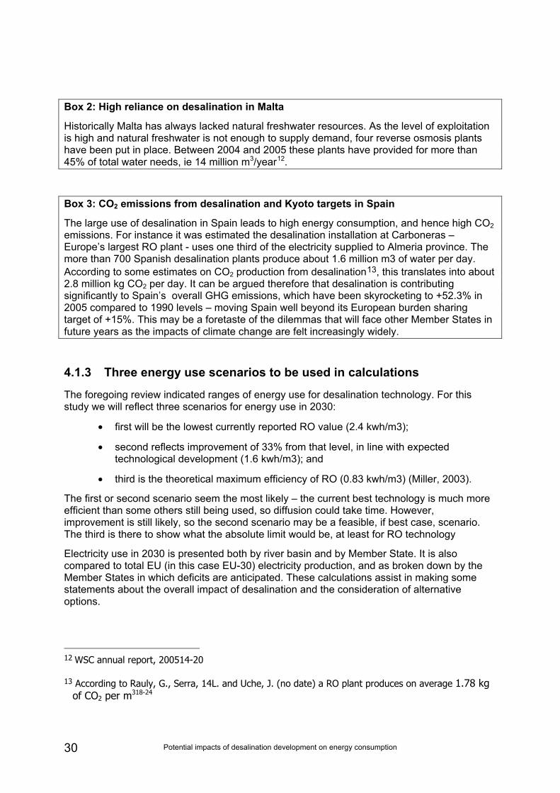
Historically Malta has always lacked natural freshwater resources. As the level of exploitation is high and natural freshwater is not enough to supply demand, four reverse osmosis plants have been put in place. Between 2004 and 2005 these plants have provided for more than 45% of total water needs, ie 14 million m3/year12.
Box 3: CO2 emissions from desalination and Kyoto targets in Spain
The large use of desalination in Spain leads to high energy consumption, and hence high CO2 emissions. For instance it was estimated the desalination installation at Carboneras – Europe’s largest RO plant - uses one third of the electricity supplied to Almeria province. The more than 700 Spanish desalination plants produce about 1.6 million m3 of water per day. According to some estimates on CO2 production from desalination13, this translates into about 2.8 million kg CO2 per day. It can be argued therefore that desalination is contributing significantly to Spain’s overall GHG emissions, which have been skyrocketing to +52.3% in 2005 compared to 1990 levels – moving Spain well beyond its European burden sharing target of +15%. This may be a foretaste of the dilemmas that will face other Member States in future years as the impacts of climate change are felt increasingly widely.
4.1.3 Three energy use scenarios to be used in calculations
The foregoing review indicated ranges of energy use for desalination technology. For this study we will reflect three scenarios for energy use in 2030:
• first will be the lowest currently reported RO value (2.4 kwh/m3);
• second reflects improvement of 33% from that level, in line with expected technological development (1.6 kwh/m3); and
• third is the theoretical maximum efficiency of RO (0.83 kwh/m3) (Miller, 2003).
The first or second scenario seem the most likely – the current best technology is much more efficient than some others still being used, so diffusion could take time. However, improvement is still likely, so the second scenario may be a feasible, if best case, scenario. The third is there to show what the absolute limit would be, at least for RO technology
Electricity use in 2030 is presented both by river basin and by Member State. It is also compared to total EU (in this case EU-30) electricity production, and as broken down by the Member States in which deficits are anticipated. These calculations assist in making some statements about the overall impact of desalination and the consideration of alternative options.
12 WSC annual report, 200514-20
13 According to Rauly, G., Serra, 14L. and Uche, J. (no date) a RO plant produces on average 1.78 kg of CO2 per m318-24
Potential impacts of desalination development on energy consumption 31
4.1.4 Energy to transport water
The distance and height rise to transport desalinated water were given in table 2 of chapter three, above.
The energy used for water transport is based primarily on the height it must rise – essentially, once the pressurization of the line and the energy to lift water is factored in, then the horizontal component is essentially negligible, in particular for the kind of estimation being done here14.
Factors used here are based on real water pumping cases (Cohen et al, 2004) with a pump efficiency of 70%, and result in a factor of 0.003885 kwh/m3 of water per metre of rise.
Calculations are then simply the multiplication of the rises indicated above and the energy use factor just noted – these results are reflected in the table below.
4.1.5 Estimating future CO2 Emissions and energy costs: based on the Primes scenarios
Carbon dioxide will be emitted to produce the energy calculated in the previous step, but how much depend on the way we assume energy will be generated in 2030. To assist in that forecast we rely on a standard model in EU energy analysis (Primes15) and its outputs for a baseline and two alternative scenarios. In this case we rely on a recent run of the Primes model produced for a Eurelectric project ‘The role of electricity16’ (scenarios are detailed in the sub-report Capros et al 2007). That report has several advantages:
• It updates the 2005 scenarios produced for the European Commission (Mantzos and Capros, 2005) by incorporating higher future fossil fuel cost assumptions – something that seems increasingly like a long term reality and which has been left out of most previous models available.
• It explicitly models alternative scenarios that match those of interest to this project: roughly compatible with Europe’s anticipated CO2 reduction commitments (-30% in 2030) , with a variety of assumptions about alternative fuel mixes.
• It provides detailed outputs that include breakdowns of electricity mixes and price projections.
The cost of electricity is provided as an EU average broken down by sector: in this case we will take the price of industrial electricity (which is generally on the order of half the price of residential electricity).
14 There is extensive literature on water movement based on the many decades of experience in
California, USA, from which these conclusions are drawn. See for example Cohen et al. (2004).
15 www.e3mlab.ntua.gr
16 www2.eurelectric.org/Content/Default.asp?PageID=729
Potential impacts of desalination development on energy consumption 32
More detail on the scenarios used
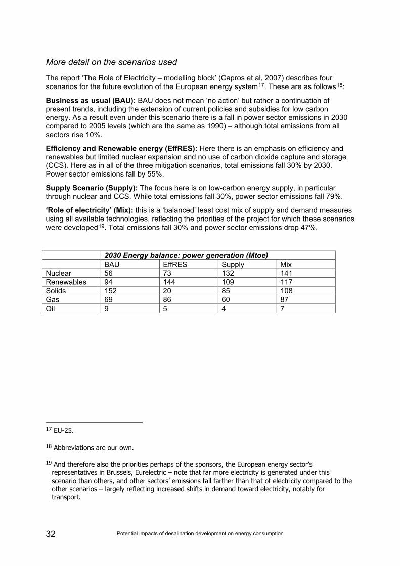
The report ‘The Role of Electricity – modelling block’ (Capros et al, 2007) describes four scenarios for the future evolution of the European energy system17. These are as follows18:
Business as usual (BAU): BAU does not mean ‘no action’ but rather a continuation of present trends, including the extension of current policies and subsidies for low carbon energy. As a result even under this scenario there is a fall in power sector emissions in 2030 compared to 2005 levels (which are the same as 1990) – although total emissions from all sectors rise 10%.
Efficiency and Renewable energy (EffRES): Here there is an emphasis on efficiency and renewables but limited nuclear expansion and no use of carbon dioxide capture and storage (CCS). Here as in all of the three mitigation scenarios, total emissions fall 30% by 2030. Power sector emissions fall by 55%.
Supply Scenario (Supply): The focus here is on low-carbon energy supply, in particular through nuclear and CCS. While total emissions fall 30%, power sector emissions fall 79%.
‘Role of electricity’ (Mix): this is a ‘balanced’ least cost mix of supply and demand measures using all available technologies, reflecting the priorities of the project for which these scenarios were developed19. Total emissions fall 30% and power sector emissions drop 47%.
2030 Energy balance: power generation (Mtoe) BAU EffRES Supply Mix Nuclear 56 73 132 141 Renewables 94 144 109 117 Solids 152 20 85 108 Gas 69 86 60 87 Oil 9 5 4 7
17 EU-25.
18 Abbreviations are our own.
19 And therefore also the priorities perhaps of the sponsors, the European energy sector’s representatives in Brussels, Eurelectric – note that far more electricity is generated under this scenario than others, and other sectors’ emissions fall farther than that of electricity compared to the other scenarios – largely reflecting increased shifts in demand toward electricity, notably for transport.
Potential impacts of desalination development on energy consumption 33
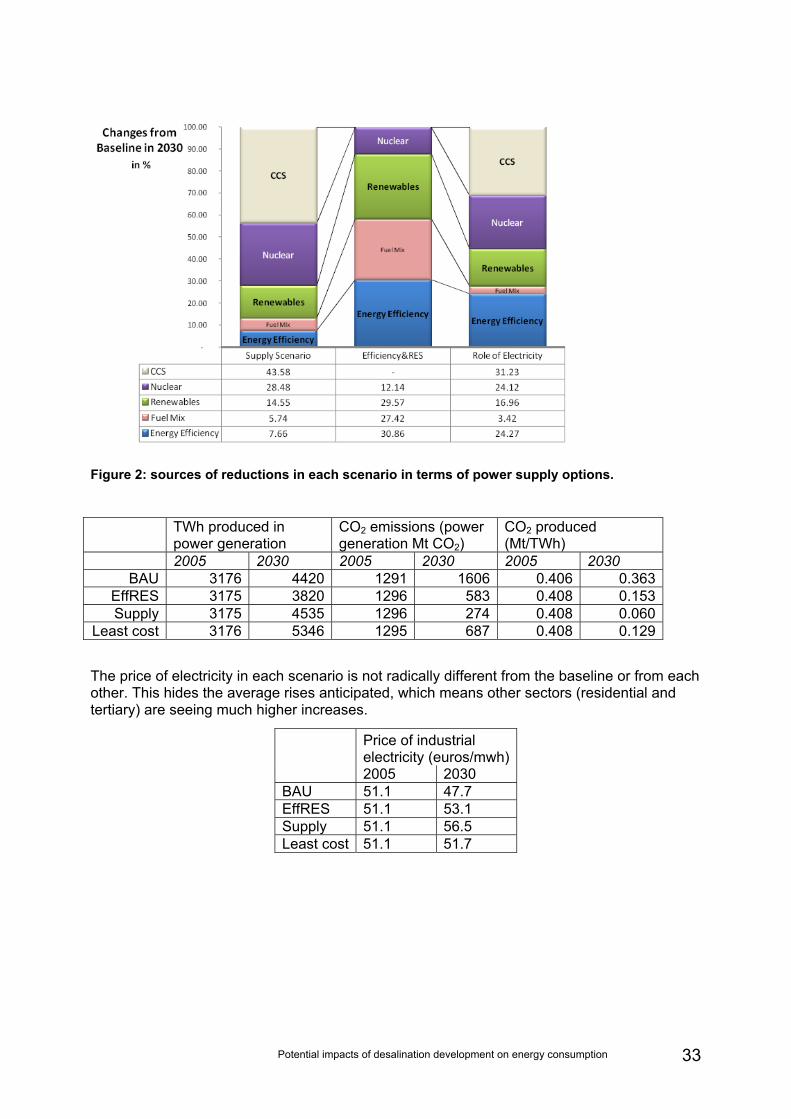
Figure 2: sources of reductions in each scenario in terms of power supply options.
TWh produced in power generation
CO2 emissions (power generation Mt CO2)
CO2 produced (Mt/TWh)
2005 2030 2005 2030 2005 2030 BAU 3176 4420 1291 1606 0.406 0.363
EffRES 3175 3820 1296 583 0.408 0.153Supply 3175 4535 1296 274 0.408 0.060
Least cost 3176 5346 1295 687 0.408 0.129
The price of electricity in each scenario is not radically different from the baseline or from each other. This hides the average rises anticipated, which means other sectors (residential and tertiary) are seeing much higher increases.
Price of industrial electricity (euros/mwh)
2005 2030 BAU 51.1 47.7 EffRES 51.1 53.1 Supply 51.1 56.5 Least cost 51.1 51.7
Potential impacts of desalination development on energy consumption 34
4.2 Presentation of Results: energy use, CO2 emissions and energy costs in 2030
4.2.1 National energy use: baseline case in 2030
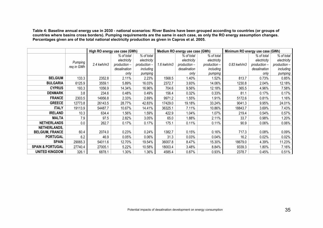
Using a detailed description of future baseline (Business as Usual)20 energy use in 2030, the amount of energy used by desalination can be ascribed to the countries in which the associated water scarcity is found. This is done here by grouping river basins in the appropriate country (where there is more than one river basin for a country). Where river basins cross border, the group of affected countries is kept together and their energy requirements are summed (e.g. the % of national energy use is as a % of the total of the countries). Table 4 displays the results.
What can be seen from this analysis is that in certain RO energy use cases and for certain countries, energy use is extremely high – e.g. Cyprus, Greece, Italy, Spain. Additionally, the energy consumption required for pumping is found to be very high in most cases. This calculation is sensitive to the assumptions made and would have to be reviewed for realism in actual cases.
In addition, however, two things can be done to do a more detailed and perhaps more realistic analysis:
1) Ascribe energy use not just to these countries but across all of Europe. The following section is based on such an averaging.
2) Consider policy scenarios where less desalination is needed due to measures to reduce the water deficit. This is considered in chapter 6.
20 In this case this data is not the same as in the subsequent analysis, but the BAU case from Capros et
al, 2005 – a report for DG Transport and Energy of the European Commission. This is because national data for Capros, 2007 has not been published.
Potential impacts of desalination development on energy consumption 35
Table 4: Baseline annual energy use in 2030 - national scenarios: River Basins have been grouped according to countries (or groups of countries where basins cross borders). Pumping requirements are the same in each case, as only the RO energy assumption changes. Percentages given are of the total national electricity production as given in Capros et al. 2005.
High RO energy use case (GWh) Medium RO energy use case (GWh) Minimum RO energy use case (GWh)
Pumping req in GWh 2.4 kwh/m3
% of total electricity
production –desalination
only
% of total electricity
production – including pumping
1.6 kwh/m3
% of total electricity
production –desalination
only
% of total electricity
production – including pumping
0.83 kwh/m3
% of total electricity
production –desalination
only
% of total electricity
production – including pumping
BELGIUM 133.3 2352.8 2.11% 2.23% 1568.5 1.40% 1.52% 813.7 0.73% 0.85% BULGARIA 6125.9 3559.1 5.89% 16.03% 2372.7 3.93% 14.06% 1230.8 2.04% 12.18%
CYPRUS 193.3 1056.9 14.34% 16.96% 704.6 9.56% 12.18% 365.5 4.96% 7.58% DENMARK 3.8 234.6 0.48% 0.49% 156.4 0.32% 0.33% 81.1 0.17% 0.17%
FRANCE 2303.5 14956.8 2.33% 2.69% 9971.2 1.55% 1.91% 5172.6 0.81% 1.16% GREECE 12773.8 26143.5 28.77% 42.83% 17429.0 19.18% 33.24% 9041.3 9.95% 24.01%
ITALY 19113.9 54487.7 10.67% 14.41% 36325.1 7.11% 10.86% 18843.7 3.69% 7.43% IRELAND 10.3 634.4 1.56% 1.59% 422.9 1.04% 1.07% 219.4 0.54% 0.57%
MALTA 7.9 97.5 2.82% 3.05% 65.0 1.88% 2.11% 33.7 0.98% 1.20% NETHERLANDS 0.0 262.7 0.17% 0.17% 175.1 0.11% 0.11% 90.9 0.06% 0.06% NETHERLANDS,
BELGIUM, FRANCE 60.4 2074.0 0.23% 0.24% 1382.7 0.15% 0.16% 717.3 0.08% 0.09% PORTUGAL 6.2 46.9 0.05% 0.06% 31.3 0.03% 0.04% 16.2 0.02% 0.02%
SPAIN 29065.3 54011.6 12.70% 19.54% 36007.8 8.47% 15.30% 18679.0 4.39% 11.23% SPAIN & PORTUGAL 27740.4 27005.1 5.22% 10.58% 18003.4 3.48% 8.84% 9339.3 1.80% 7.16%
UNITED KINGDOM 326.1 6878.1 1.30% 1.36% 4585.4 0.87% 0.93% 2378.7 0.45% 0.51%
Potential impacts of desalination development on energy consumption 36
4.2.2 European energy, CO2 emissions, costs and future scenarios
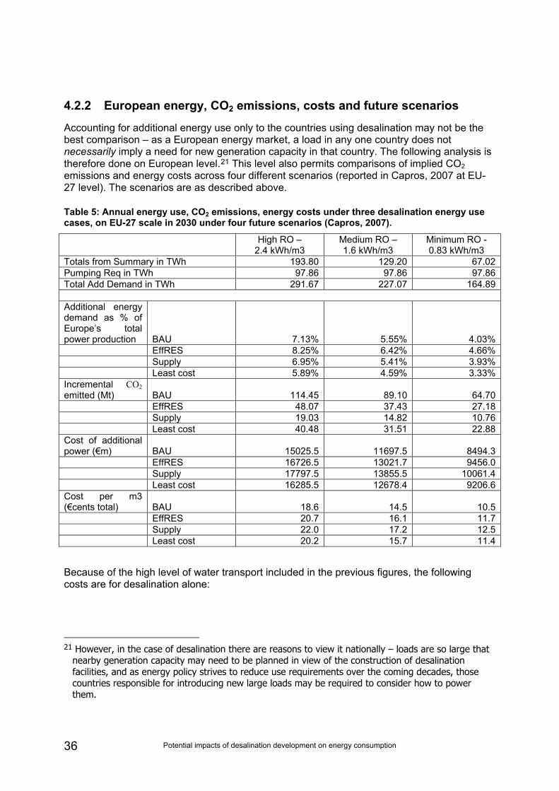
Accounting for additional energy use only to the countries using desalination may not be the best comparison – as a European energy market, a load in any one country does not necessarily imply a need for new generation capacity in that country. The following analysis is therefore done on European level.21 This level also permits comparisons of implied CO2 emissions and energy costs across four different scenarios (reported in Capros, 2007 at EU-27 level). The scenarios are as described above.
Table 5: Annual energy use, CO2 emissions, energy costs under three desalination energy use cases, on EU-27 scale in 2030 under four future scenarios (Capros, 2007).
High RO –
2.4 kWh/m3 Medium RO – 1.6 kWh/m3
Minimum RO - 0.83 kWh/m3
Totals from Summary in TWh 193.80 129.20 67.02Pumping Req in TWh 97.86 97.86 97.86Total Add Demand in TWh 291.67 227.07 164.89 Additional energy demand as % of Europe’s total power production BAU 7.13% 5.55% 4.03% EffRES 8.25% 6.42% 4.66% Supply 6.95% 5.41% 3.93% Least cost 5.89% 4.59% 3.33%Incremental CO2 emitted (Mt) BAU 114.45 89.10 64.70 EffRES 48.07 37.43 27.18 Supply 19.03 14.82 10.76 Least cost 40.48 31.51 22.88Cost of additional power (€m) BAU 15025.5 11697.5 8494.3 EffRES 16726.5 13021.7 9456.0 Supply 17797.5 13855.5 10061.4 Least cost 16285.5 12678.4 9206.6Cost per m3 (€cents total) BAU 18.6 14.5 10.5 EffRES 20.7 16.1 11.7 Supply 22.0 17.2 12.5 Least cost 20.2 15.7 11.4
Because of the high level of water transport included in the previous figures, the following costs are for desalination alone:
21 However, in the case of desalination there are reasons to view it nationally – loads are so large that
nearby generation capacity may need to be planned in view of the construction of desalination facilities, and as energy policy strives to reduce use requirements over the coming decades, those countries responsible for introducing new large loads may be required to consider how to power them.
Potential impacts of desalination development on energy consumption 37
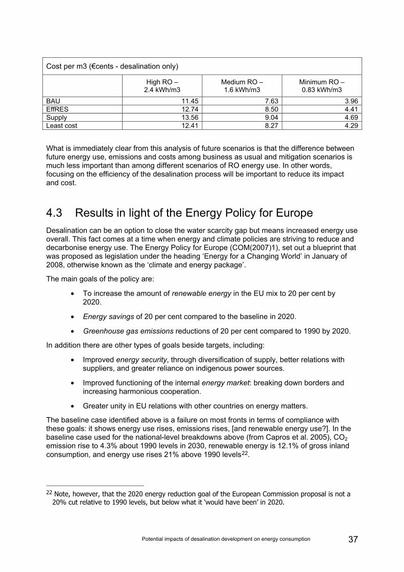
Cost per m3 (€cents - desalination only)
High RO – 2.4 kWh/m3
Medium RO – 1.6 kWh/m3
Minimum RO – 0.83 kWh/m3
BAU 11.45 7.63 3.96EffRES 12.74 8.50 4.41Supply 13.56 9.04 4.69Least cost 12.41 8.27 4.29
What is immediately clear from this analysis of future scenarios is that the difference between future energy use, emissions and costs among business as usual and mitigation scenarios is much less important than among different scenarios of RO energy use. In other words, focusing on the efficiency of the desalination process will be important to reduce its impact and cost.
4.3 Results in light of the Energy Policy for Europe Desalination can be an option to close the water scarcity gap but means increased energy use overall. This fact comes at a time when energy and climate policies are striving to reduce and decarbonise energy use. The Energy Policy for Europe (COM(2007)1), set out a blueprint that was proposed as legislation under the heading ‘Energy for a Changing World’ in January of 2008, otherwise known as the ‘climate and energy package’.
The main goals of the policy are:
• To increase the amount of renewable energy in the EU mix to 20 per cent by 2020.
• Energy savings of 20 per cent compared to the baseline in 2020.
• Greenhouse gas emissions reductions of 20 per cent compared to 1990 by 2020.
In addition there are other types of goals beside targets, including:
• Improved energy security, through diversification of supply, better relations with suppliers, and greater reliance on indigenous power sources.
• Improved functioning of the internal energy market: breaking down borders and increasing harmonious cooperation.
• Greater unity in EU relations with other countries on energy matters.
The baseline case identified above is a failure on most fronts in terms of compliance with these goals: it shows energy use rises, emissions rises, [and renewable energy use?]. In the baseline case used for the national-level breakdowns above (from Capros et al. 2005), CO2 emission rise to 4.3% about 1990 levels in 2030, renewable energy is 12.1% of gross inland consumption, and energy use rises 21% above 1990 levels22.
22 Note, however, that the 2020 energy reduction goal of the European Commission proposal is not a
20% cut relative to 1990 levels, but below what it ‘would have been’ in 2020.
Potential impacts of desalination development on energy consumption 38
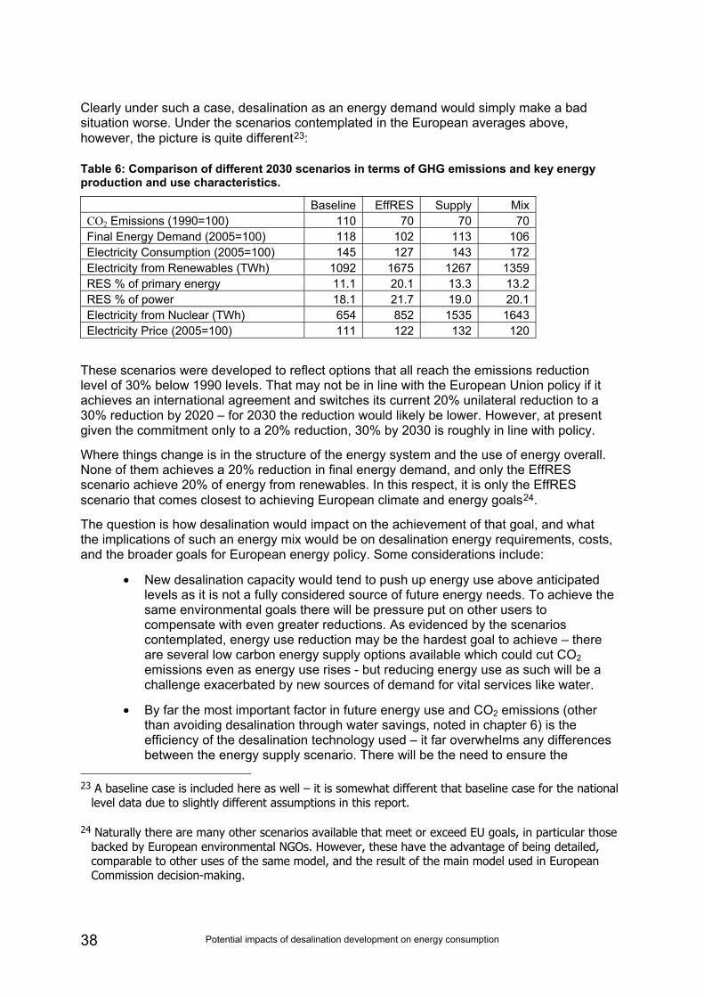
Clearly under such a case, desalination as an energy demand would simply make a bad situation worse. Under the scenarios contemplated in the European averages above, however, the picture is quite different23:
Table 6: Comparison of different 2030 scenarios in terms of GHG emissions and key energy production and use characteristics.
Baseline EffRES Supply Mix CO2 Emissions (1990=100) 110 70 70 70 Final Energy Demand (2005=100) 118 102 113 106 Electricity Consumption (2005=100) 145 127 143 172 Electricity from Renewables (TWh) 1092 1675 1267 1359 RES % of primary energy 11.1 20.1 13.3 13.2 RES % of power 18.1 21.7 19.0 20.1 Electricity from Nuclear (TWh) 654 852 1535 1643 Electricity Price (2005=100) 111 122 132 120
These scenarios were developed to reflect options that all reach the emissions reduction level of 30% below 1990 levels. That may not be in line with the European Union policy if it achieves an international agreement and switches its current 20% unilateral reduction to a 30% reduction by 2020 – for 2030 the reduction would likely be lower. However, at present given the commitment only to a 20% reduction, 30% by 2030 is roughly in line with policy.
Where things change is in the structure of the energy system and the use of energy overall. None of them achieves a 20% reduction in final energy demand, and only the EffRES scenario achieve 20% of energy from renewables. In this respect, it is only the EffRES scenario that comes closest to achieving European climate and energy goals24.
The question is how desalination would impact on the achievement of that goal, and what the implications of such an energy mix would be on desalination energy requirements, costs, and the broader goals for European energy policy. Some considerations include:
• New desalination capacity would tend to push up energy use above anticipated levels as it is not a fully considered source of future energy needs. To achieve the same environmental goals there will be pressure put on other users to compensate with even greater reductions. As evidenced by the scenarios contemplated, energy use reduction may be the hardest goal to achieve – there are several low carbon energy supply options available which could cut CO2 emissions even as energy use rises - but reducing energy use as such will be a challenge exacerbated by new sources of demand for vital services like water.
• By far the most important factor in future energy use and CO2 emissions (other than avoiding desalination through water savings, noted in chapter 6) is the efficiency of the desalination technology used – it far overwhelms any differences between the energy supply scenario. There will be the need to ensure the
23 A baseline case is included here as well – it is somewhat different that baseline case for the national
level data due to slightly different assumptions in this report.
24 Naturally there are many other scenarios available that meet or exceed EU goals, in particular those backed by European environmental NGOs. However, these have the advantage of being detailed, comparable to other uses of the same model, and the result of the main model used in European Commission decision-making.
Potential impacts of desalination development on energy consumption 39
adoption of minimum standards of energy efficient desalination technology. A side benefit could be the opening of new markets for eco-technologies in the EU (even though, at the outset at least, EU industry will face tough competition with exports coming from countries where the technology has a long history of deployment and high levels of sophistication, like Israel).
• Water resources are necessarily location-specific, which may on balance lead to some more inertia in the decoupling of location from energy market supply as Europe moves towards a single market not just on paper but in terms of the free flow of electrons. New centres of major energy requirements, depending on their locations, may require dedicated energy transmission lines, and could put stress on segments of the integrated electricity grid which may not be connected with high capacities to other segments (bottlenecks to the Iberian Peninsula are currently evident for example, which is a likely location of future desalination).
• Energy use for desalinisation within certain Member States may create pressure to allow softer energy targets when negotiating future target sharing agreements, as fresh water availability is an important need. The current ‘effort sharing’ approach does not factor in variations in national conditions – not only for water but even for such tings as heating and cooling load – so at present this is not a consideration, but could emerge in future depending on the success of the currently proposed approach.
• Relying increasingly on energy to create all-important fresh water would link two vital resources together – water and energy. It is potentially risky to have our water supply linked to energy, which itself has security issues. Desalination could thus magnify energy security problems through the link to water use. Those energy supply strategies relying more heavily on indigenous resources – such as those with an emphasis efficiency and renewable energy – may yield a double advantage in the security perspective – both energy and water.
This report simply treats desalination as another source of electricity demand without differentiating specific effects on the energy system – a level of detail that seems premature on the basis of these broad-brush estimates. Fundamentally, though, an increase in Europe’s electricity requirements by between 3 and 7% to meet desalination and transport requirements is a large-scale challenge. One of the important means to meet it will be to focus on the means of reducing the energy requirement of desalination, which is explored in chapter 6.

Potential impacts of desalination development on energy consumption 40
5 Financial feasibility of desalination
5.1 An indicator for measuring the financial feasibility It has been assumed so far in this report that the desalination-only option for tackling future water deficits would be both technical and financially feasible. However, with the order of magnitude of the volumes to be desalinated and the associated costs for desalination and transport, financial feasibility needs to be further checked in particular, whether the desalination-only option would entail disproportionate costs25 as compared to what people are paying today for water.
The approach chosen here concentrates on the likely impacts of desalination costs on water prices and the water bill, assuming that all additional costs linked to desalination are entirely passed to water consumers. In that context, the relative share of the water bill in household’s total disposable income is used as the indicator for assessing financial feasibility, comparing the value of the indicator estimated for each river basin with a given threshold (2%26 or 4%27). If the share of the bill in the total disposable income is higher than these threshold values, the desalination option is then considered disproportionately costly and financially infeasible.
It should be stressed that this assessment is made for households only. Although water use by agriculture is larger than water use by households, water pricing in the agriculture sector is still highly subsidised. As a result, it would be unclear whether additional costs resulting from the desalination-only option would be passed to agriculture water users or would be subsidised, making any assessment highly uncertain.
The calculation of the chosen indicator for households implies that the water bill and household income is known for each river basin. The water bill that will be used to do the comparison with household disposable income will build on:
• The current water price;
• An estimation of the “baseline” water price by 2030, taking into account all additional costs linked to the implementation of existing water directives (for example, the Urban Waste Water Treatment Directive (UWWTD) or the Drinking Water Directive (DWD)) that will take place in the coming years and that will need to be paid for by water users;
25 The term disproportionate costs directly originates from the EU WFD text. It is used in the context of
time/objective exemptions that might be justified if costs a considered disproportionate. One of the assessments that is discussed in this context is the comparison between costs of proposed measures (in our case: desalination) and the costs that water users already pay as part of their water bill.
26 Courtecuisse (2005); quoting three sources: EU Commission and Académie de l'eau
27 OECD (2004)
Potential impacts of desalination development on energy consumption 41
• The cost of desalination (including transport costs the costs linked to the process and the costs linked to the transport) which will lead to increases in the “baseline” price;
• Water consumption by households.
5.2 The method The calculation of the parameters listed above required several sources of information and several calculations. The main steps and choices are presented below with references to annexes for further details.
5.2.1 Water prices
Current water price
In most of the countries, current water prices are composed of four components:
• A fixed charge per year – independent of the level of consumption;
• A variable charge per m3 for the distribution and purification of drinking water per m3;
• A charge for sewerage and wastewater treatment; and,
• VAT and taxes.
Courtecuisse (2007) states in his study that most of those components are the result of local decisions (except for VAT and national taxes) leading to significant differences between water supply areas even within shorter distances28. The main factors explaining these differences include topography, current investments, standards of services or the seasonality of the water demand. Despite these, an attempt is made to estimate average water prices for each river basin, using the average value of different cities of the basin obtained from data of the International Water Association or, when such values are not available for a given basin, the national average price. Calculation details are given in Annex A.
Future water price
As indicated above, it is assumed that prices in 2030 will differ from today’s water prices because of the implementation of existing European environmental legislation and its impact on the water sector (e.g. implementation of the UWWTD, DWD or Water Framework Directive including its cost-recovery requirements). It is assumed that the largest price increase will still come from the implementation of the UWWTD (see Annex B) as it has been the case for the last 40 years with the provision of wastewater treatment of urban and industrial sewage discharges accounting for 50-60% of total investments in environmental protection in industrialized countries” (EEA 2005). It is assumed that the application of the polluter-pays- 28 The same study on water prices discovered for the Artois Picardie river basin in France that price differences up to 2 €/m3 can occur even within the same river basin (Courtecuisse 2007)
Potential impacts of desalination development on energy consumption 42
principle and cost-recovery will become stricter in most countries as a result of the implementation of the WFD, resulting in all costs being passed to water consumers29. It is also assumed that the costs for renewing existing infrastructure are already included in today’s water prices and will be covered with normal water price increases.
Different methods were compared to estimate future water prices estimated on the basis of compliance with the UWWTD (see Annex B). To apply a ratio of 1:1.4 between drinking water charges and wastewater charges was chosen as the most appropriate method for calculating the effect on total water prices of implementing the UWWTD, this application resulting mainly in an increase in total water bill for countries with a more limited implementation of the obligations of the UWWTD (in particular, Member States which have joined the EU since 2004).
5.2.2 Desalination costs
The production of desalted water
During the last 50 years there has been a steady growth of desalination plants. Today, the worldwide installed capacity has gone past 30 million m3 of desalted water per day.There are two main desalination processes: thermal (MED (Multi-Effect-Distillation), MSF (Multi-Stage-Flash)) and Reverse Osmosis (RO). Historically, the thermal processes were the first to be developed. RO technology was developed later, mainly during the 70s. Nowadays, the capacity of each technology is more or less equal. Nevertheless, with the growth of membrane science, RO overtook MSF as the leading desalination technology, and is then considered as the chosen technology (Miller 2003) for which costs can be assessed.
Estimates of investment costs and operation & maintenance costs have been found in the literature (e.g. Zhou & Tol 2004, Chaudhry 2003, Ebensperger & Isley 2005). Their review shows that:
• The cost to desalted water has been decreasing over time (despite rising energy prices) as a result of technology change and economy of scales (Zhou & Tol 2004, Chaudhry 2003, Miller 2003, Ebensperger & Isley 2005, World Bank 2004, Fritzmann et al. 2006);
• Today, the average cost of RO desalination ranges between 0.35 and 0.7€/m3 of desalted water (Zhou & Tol 2004, Chaudhry 2003, Miller 2003, Ebensperger & Isley 2005, World Bank 2004, Fritzmann et al. 2006);
• There are economies of scale with the size of investments (Chaudhry 2003, Miller 2003, World Bank 2004, Fritzmann et al. 2006, Metaiche & Kettab 2005);
• Energy consumption of larger plants is lower (Miller 2003);
• Desalination of brackish water is cheaper than desalination of seawater both in terms of investment and energy costs (Chaudhry 2003, Miller 2003, World Bank 2004, Fritzmann et al. 2006).
29 Still it has to be taken into account that funding possibilities exist for certain countries concerning investment costs in the wastewater sector. But operating and maintenance costs as well as the replacement of facilities have to be covered by the member states themselves.
Potential impacts of desalination development on energy consumption 43
Several methods were identified to estimate the cost of a desalination plants (for example, see World Bank 2004 and Fritzmann et al. 2006, Miller 2003). Taking into account the large amounts of water which will have to be desalinated to fill the water gap by 2030, costs for large desalination plants have been chosen. It is assumed that desalination plants with a daily capacity of 100 000 m3/day will be constructed, resulting in an average value of desalination costs of 0.25 €/m3.
Distribution costs
Literature about transportation costs is rather poor. Zhou and Tol (2006) only provide references to average transportation costs (based on Kally, 1993) combining vertical cost (pumping cost mainly) and horizontal costs (costs of pipes). As an average, the costs to transport 1 m3 of water is estimated at 0.037 € per 100 m of vertical transport and 0.043 € per 100 km of horizontal transport. These unitary cost values are then applied to transport routes defined for each river basin and presented in the previous chapters.
Other Costs
Other costs, related to the pre-treatment and the concentrate disposal, can also be considered. If they are often mentioned in the literature, very few articles give orders of magnitudes of these costs. Miller (2003) estimates pre-treatment costs to account for up to 30% of O&M costs while Younos (2004) estimates the costs of brine disposal between 5 to 33% of total costs. These costs will not be considered further.
Effect of desalination on water prices
The total cost of 1 m3 of desalted water (pdesa ) is then the future “baseline” water price (p2030) plus the additional cost linked to the desalination (Δdesa), including desalination process and transport.
pdesa = p2030 + Δdesa
Whereby: pdesa= Price of desalted water
p2030 = Future water price without additional desalination (but including the level of desalination today)
Δdesa = Additional costs to desalinate water, including transport costs
The desalted water only constitutes part of the future water supply which is the water deficit. The increase in the future water price is therefore proportionate to the share of this water deficit. The following formula was used to determine the future water price (p2030+desa) for each river basin:
p2030+desa = [pdesa * WD2030 + p2030 (WA2030 – WD2030)] / WA2030
Potential impacts of desalination development on energy consumption 44
Whereby: p2030+desa = New water, taking into account that part of the water consumed stems from additional desalination
WD2030 = Water deficit 2030
WA2030 = Water abstraction / consumption 2030
5.2.3 Water consumption in households
Household water consumptions were calculated using water consumption per capita from Courtecuisse (2005) and average household sizes found in United Nations Economic Commission for Europe (UNECE, 2004). More details are provided in Annex C. As a first approximation, these figures are used also for the 2030 household water consumptions.
5.2.4 Net disposable household income
Current income
Data about household incomes were found at NUTS 230 level in Eurostat database (Eurostat 2005). Some calculations were made to adapt values at the river basin level as indicated in Annex D.
Future income – growth projections
Future household income is expected to be related to economic growth. Different projection values were found for future GDP growth for European countries. All studies, despite analysing different time scales, provided economic growths in similar ranges. This factor has however not been considered for our calculations.
5.3 Results Estimated water prices
Current water prices
Current water prices are highly variable between river basins (see Annex E). The highest value, 4.27 €/m3 (Zealand river basin in Denmark) is approximately tenfold higher than the lowest value, 0.49 €/m3 (West and East Aegean river basins in Bulgaria). The average water price is 1.74 €/m3. In Ireland, the domestic sector does not pay for water services via water charges, as water charges for households have been abolished in 1998 (EPA 2005).
Future water prices to account for the implementation of the UWWTD
Future water prices that were estimated are shown in Annex F. Only four river basins had currently a higher ratio than 1:1.4 between drinking water and wastewater charges. Whereas the values for Denmark and the Anglian river basin in the UK differ only with a few cents, the ratio of the price components in Cyprus today is already 1:3.1. In the Jucar basin in Spain, the 30 NUTS – ‘Nomenclature des unités territoriales statistiques’ ; NUTS 2 : Medium regions / landscapes
Potential impacts of desalination development on energy consumption 45
current wastewater charge of 0.59 €/m3 is 0.21 €/m3 higher than the 1:1.4 ratio. In these cases, future water prices to account for the implementation of the UWWTD have been kept equal to today’s water prices. Estimated future water prices range from 0.86 €/m3 (Cental Appennines, Italy) to 4.27 €/m3 (Zealand, Denmark). The average value for future water prices accounting for the implementation of the UWWTD is 2.18 €/m3.
Effect of desalination
The effect of desalination on water price is rather small. Indeed, total water prices including the costs of desalination are expected to range from 0.99 €/m3 (West Aegan, Bulgaria and Central Appennines, Italy) to 4.39 €/m3 (Zealand, Denmark). The average water price would then be 2.34 €/m3, with an average increase of around 0.1€/m3 as compared to future water prices.
Share of the water bill in the household income
The following table summarises the main results of the final calculations. Its first columns present the share of the water bill in total household disposable income for (a) current water prices, (b) future “baseline” water prices and (c) future baseline water prices plus desalination costs. As mention before, water consumption, household income and the number of household members are assumed to be constant over the time period considered. The table shows that the desalination-only option has a rather limited impact on the share of the water bill in the total disposable income. Indeed, only three basins are reaching the 2% threshold value proposed above: the Western Sterea Elada and Northern Peloponnese in Greece (2.0%) and the Sadothe & Mira basins in Portugal (2.1%). However, the relative share of the water bill in total disposable income would already reach this threshold with estimated future “baseline” prices, stressing the most significant importance of costs of the UWWTD.
A significant increase in the relative importance of the water bill would be recorded for some basins only: Central Appennines, Italy (+18%); Tajo and Duoro, Spain/Portugal (+17%); Jucar, Segura, Guadalquivir and Ebro, Spain (from +18% to +25%); Malta (+23%) and West Aegan, Bulgaria (+54%). However, water bills would remain below the 2% threshold of total disposable income for these basins.
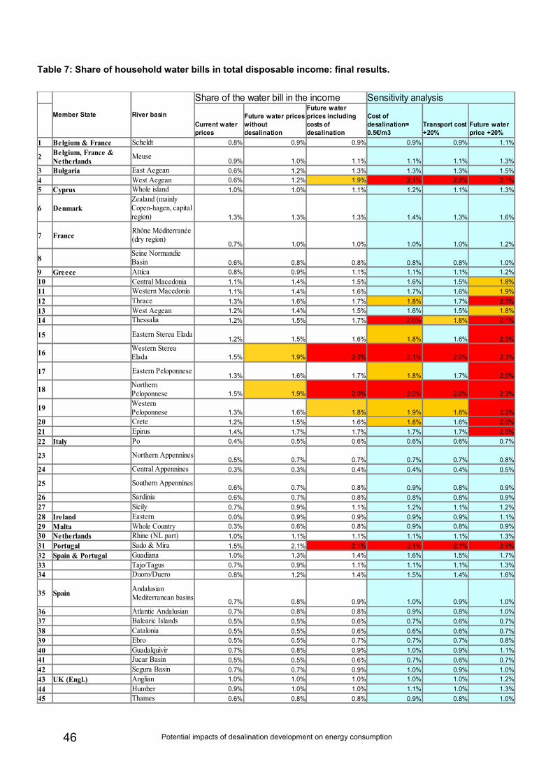
Potential impacts of desalination development on energy consumption 46
Member State River basin
Share of the water bill in the income Sensitivity analysis
1 Belgium & France Scheldt 0.8% 0.9% 0.9% 0.9% 0.9% 1.1%
2 Meuse0.9% 1.0% 1.1% 1.1% 1.1% 1.3%
3 Bulgaria East Aegean 0.6% 1.2% 1.3% 1.3% 1.3% 1.5%4 West Aegean 0.6% 1.2% 1.9% 2.1% 2.0% 2.1%5 Cyprus Whole island 1.0% 1.0% 1.1% 1.2% 1.1% 1.3%
6 Denmark1.3% 1.3% 1.3% 1.4% 1.3% 1.6%
7 France0.7% 1.0% 1.0% 1.0% 1.0% 1.2%
8 0.6% 0.8% 0.8% 0.8% 0.8% 1.0%9 Greece Attica 0.8% 0.9% 1.1% 1.1% 1.1% 1.2%10 Central Macedonia 1.1% 1.4% 1.5% 1.6% 1.5% 1.8%11 Western Macedonia 1.1% 1.4% 1.6% 1.7% 1.6% 1.9%12 Thrace 1.3% 1.6% 1.7% 1.8% 1.7% 2.0%13 West Aegean 1.2% 1.4% 1.5% 1.6% 1.5% 1.8%14 Thessalia 1.2% 1.5% 1.7% 2.0% 1.8% 2.1%
15 Eastern Sterea Elada1.2% 1.5% 1.6% 1.8% 1.6% 2.0%
16 1.5% 1.9% 2.0% 2.1% 2.0% 2.3%
17 Eastern Peloponnese1.3% 1.6% 1.7% 1.8% 1.7% 2.0%
18 1.5% 1.9% 2.0% 2.0% 2.0% 2.3%
19 1.3% 1.6% 1.8% 1.9% 1.8% 2.2%20 Crete 1.2% 1.5% 1.6% 1.8% 1.6% 2.0%21 Epirus 1.4% 1.7% 1.7% 1.7% 1.7% 2.0%22 Italy Po 0.4% 0.5% 0.6% 0.6% 0.6% 0.7%
23 Northern Appennines0.5% 0.7% 0.7% 0.7% 0.7% 0.8%
24 Central Appennines 0.3% 0.3% 0.4% 0.4% 0.4% 0.5%
25 Southern Appennines0.6% 0.7% 0.8% 0.9% 0.8% 0.9%
26 Sardinia 0.6% 0.7% 0.8% 0.8% 0.8% 0.9%27 Sicily 0.7% 0.9% 1.1% 1.2% 1.1% 1.2%28 Ireland Eastern 0.0% 0.9% 0.9% 0.9% 0.9% 1.1%29 Malta Whole Country 0.3% 0.6% 0.8% 0.9% 0.8% 0.9%30 Netherlands Rhine (NL part) 1.0% 1.1% 1.1% 1.1% 1.1% 1.3%31 Portugal Sado & Mira 1.5% 2.1% 2.1% 2.1% 2.1% 2.5%32 Spain & Portugal Guadiana 1.0% 1.3% 1.4% 1.6% 1.5% 1.7%33 Tajo/Tagus 0.7% 0.9% 1.1% 1.1% 1.1% 1.3%34 Duoro/Duero 0.8% 1.2% 1.4% 1.5% 1.4% 1.6%
35 Spain0.7% 0.8% 0.9% 1.0% 0.9% 1.0%
36 Atlantic Andalusian 0.7% 0.8% 0.8% 0.9% 0.8% 1.0%37 Balearic Islands 0.5% 0.5% 0.6% 0.7% 0.6% 0.7%38 Catalonia 0.5% 0.5% 0.6% 0.6% 0.6% 0.7%39 Ebro 0.5% 0.5% 0.7% 0.7% 0.7% 0.8%40 Guadalquivir 0.7% 0.8% 0.9% 1.0% 0.9% 1.1%41 Jucar Basin 0.5% 0.5% 0.6% 0.7% 0.6% 0.7%42 Segura Basin 0.7% 0.7% 0.9% 1.0% 0.9% 1.0%43 UK (Engl.) Anglian 1.0% 1.0% 1.0% 1.0% 1.0% 1.2%44 Humber 0.9% 1.0% 1.0% 1.1% 1.0% 1.3%45 Thames 0.6% 0.8% 0.8% 0.9% 0.8% 1.0%
Current water prices
Future water prices without desalination
Future water prices including costs of desalination
Cost of desalination= 0.5€/m3
Transport cost +20%
Future water price +20%
Belgium, France & Netherlands
Zealand (mainly Copen-hagen, capital region)
Rhône Méditerranée (dry region)
Seine Normandie Basin
Western Sterea Elada
Northern PeloponneseWestern Peloponnese
Andalusian Mediterranean basins
Table 7: Share of household water bills in total disposable income: final results.
Potential impacts of desalination development on energy consumption 47
A sensitivity analysis was made on selected factors influencing the relative share of the water bill in total disposable income. The impact of increases in desalination costs (+100% up to 0.5 €/m3), in transport costs (+20%) and future water price as a result of the implementation of the UWWTD (+20%) on the water bill was estimated. Overall; such significant cost increases would only bring selected additional basins above the 2% threshold, mainly from Greece and Portugal. The largest impact was linked to increases in future water prices resulting from the implementation of the UWWTD.
5.4 Conclusion: high overall costs, but not at household level
Overall, and while the total costs of the desalination-only option appears as significant in absolute terms, they would only impact marginally household water bills. As a result, the total water bill as compared to household disposable income would remain below, or close to, the 2% threshold proposed for this indicator. This indicates that the desalination option appears as financially feasible and not disproportionately expensive as compared to today’s water prices and other costs imposed by the implementation of the water regulation. Large differences, however, might exist within river basins as indicated above. More detailed analysis within river basins, however, is out of the scope of the present study.
Potential impacts of desalination development on energy consumption 48
6 The impact of water savings measures on energy use
6.1 The impact of water savings measures on desalination requirements
As described in section 2 the water deficits are based on calculations made within the WATERGAP model. The model is based on several assumptions which include some efficiency developments over the time, but no specific water saving policy.
In the following section two scenarios assuming that a water saving policy exists are described. The assumptions made are based on the EU communication on water scarcity and droughts and the background study “The EU water saving potential” (Ecologic, et al, 2007).
The Commission has thus identified an initial set of policy options to be taken at European, national and regional levels to address water scarcity and droughts and mitigate their impacts within the Union. The set of proposed policies on water aims to move the EU towards a water-efficient and water-saving economy.
The communication on Water Scarcity and Droughts focuses on integrated approach to addressing water scarcity and droughts and proposes a combination of options that could be taken to reduce droughts and water scarcity. The present Communication already contains some initial proposals on how to combat water scarcity and drought on a European, national and regional level:
• Full implementation of the Water Framework Directive (WFD), which in this context should be especially addressed to the “mismanagement of water resources”. The latter often results from inefficient water pricing, which fails to reflect the real expenses of local water supply.
• introduce the “user pays” principle (beyond the sectors of water supply and wastewater treatment). In this case, the Commission explicitly supports the use of market instruments in the environmental sector, among other things referring to Articles 9 and 11 (systematic monitoring of water abstraction) of the WFD. Moreover, it underpins the importance of access to adequate water supply for private households irrespective of the means available to them.
• Better land-use planning, especially in river catchment areas, to counteract the imbalance of water allocation among different economic sectors. Local water resources have become particularly burdened by agricultural irrigation systems, which shall be curbed through further CAP reforms. It also needs to be examined what impact the growing use of biofuels has on water availability.
• Making use of the huge water savings potential, in all sectors
• A precondition for the creation of a water saving culture is the large-scale integration of supply issues in the political strategies for sectors using water. Other priority factors include information (e.g. how much water is needed for the manufacturing of a specific product) and education.
Potential impacts of desalination development on energy consumption 49
As a background to the Communication, the European Commission committed a study to identify the European water saving potential (Ecologic et al, 2007). The study addresses the savings that can by achieved via technical measures without major changes in human behaviour or production patterns. Furthermore, it looks towards instruments such as water pricing, drought management plans or labelling that can foster the implementation of these measures.
The report concentrates on the four main water users, namely public water supply (including households), agriculture, industry and tourism. It is based on a large literature review and data synthesis of existing studies and experiences of water savings in Europe but also outside Europe (e.g. Australia)31. The results with regard to water saving can be summarised as follows:
• As regards public water supply (including households, public sector and small businesses), the reduction of leakage in water supply networks, water saving devices and more efficient household appliances have the potential for up to 50% water savings. These water saving technologies are easy to introduce and implement and they also have short payback periods, further enhancing their uptake possibilities. Applying the above mentioned measures would allow for a reduction in water consumption from 150 litres/person/day (average in the EU) to a low 80 litres/person/day. A similar reduction could be applied to public water supply, leading to an estimate of potential saving up to 33% of today’s abstraction.
• In agriculture, water savings can be carried out with improvements in irrigation infrastructure and technologies. Potential water savings resulting from improvements in the conveyance efficiency of irrigation systems ranges between 10 to 25% of their water withdrawals. Water savings resulting from improving application efficiency are estimated at 15% to 60% of water use. Additional water savings can be expected from changes in irrigation practices (30%), use of more drought-resistant crops (up to 50%) or reuse of treated sewage effluent (around 10%). The potential water savings in the irrigation sector would amount to 43% of the current agricultural volume abstracted.
• Industries that use large amounts of water include the paper & pulp, textile, leather (tanning), oil and gas, chemical, pharmaceutical, food, energy, metal and mining sub-sectors. Based on the examples found the application of technical measures (e.g. changes in processes leading to less water demand, higher recycling rates or the use of rainwater) can lead to estimated savings between 15 and 90% with an global estimate up to 43% of today's water abstraction. A particular sub-sector of industry is electricity production. Electricity production uses large quantities of water for abstracting fuel and for cooling purposes in thermoelectric power plants. However, as usually a large proportion of the water abstracted in the energy sector flows back to the local environment, the benefits of water saving in this sector is marginal; therefore the global estimate of the total EU water saving potential does not involve this sector.
• The tourism sector can represent a key water user in some areas of Europe. Technical water saving measures for the tourism sector are similar to those for
31 This literature review is complemented by four detailed case studies in Spain, Greece, the UK and
France that illustrate the feasibility of implementation and likely impacts of potential water savings measures.
Potential impacts of desalination development on energy consumption 50
households. The sector has the potential to increase water use efficiency significantly by installing newer appliances in guest rooms, cafe areas, kitchens, etc. Since some of the measures identified in the report show a potential for a maximum of 80-90% savings, tourist accommodations could considerably reduce costs by buying more efficient appliances that only have payback periods of 3 years or less. In the case of irrigation of golf courses and sporting areas, more efficient irrigation techniques or rain water harvesting could provide additional savings up to 70%.
However it is important to note two issues:
− The figures presented above vary widely across the different river basins and might be higher or lower.
− The assumptions made in the water saving study are assumed to be achievable by using technical measures, only. The study does not consider major changes in human behaviour, production patterns or restrictions in land use. If measures in this area would be applied the savings can be assumed as even higher.
Based on the above presented findings two scenarios have been developed, one assuming a 20% saving and one a 40% saving. Both numbers are currently discussed in the political process (see European Commission Press release IP/07/1121 of 18/07/2007). Both scenarios have the underlying assumption that the EU sets binding reduction targets for water consumption/use in river basins facing water stress. Member States following the subsidiary principle have to implement these given target by applying the measures outlined in the Communication in their most appropriate way. In other words, Member States are free to choose from the set of measures and the way how they implement them on the national level. Such a scenario allows Member States to set their own priorities and to adapt to local circumstances accounting for the different sectoral water uses in each river basin.
These reduction cases are incorporated into the energy use calculations displayed in chapter 4 to yield the following summary tables for the baseline and reduction scenarios – these are the same as in chapter 4, with the addition of 20 and 40% reduction cases for comparison:
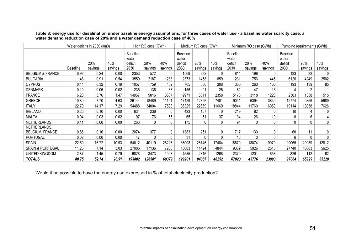
Potential impacts of desalination development on energy consumption 51
Table 8: energy use for desalination under baseline energy assumptions, for three cases of water use - a baseline water scarcity case, a water demand reduction case of 20% and a water demand reduction case of 40%
Water deficits in 2030 (km3) High RO case (GWh) Medium RO case (GWh) Minimum RO case (GWh) Pumping requirements (GWh)
Baseline 20% savings
40% savings
Baseline water deficit 2030
20% savings
40% savings
Baseline water deficit 2030
20% savings
40% savings
Baseline water deficit 2030
20% savings
40% savings
Baseline water deficit 2030
20% savings
40% savings
BELGIUM & FRANCE 0.98 0.24 0.00 2353 572 0 1569 382 0 814 198 0 133 32 0 BULGARIA 1.48 0.91 0.54 3559 2187 1288 2373 1458 859 1231 756 445 6126 4249 2502 CYPRUS 0.44 0.32 0.19 1057 759 462 705 506 308 365 263 160 193 139 85 DENMARK 0.10 0.06 0.02 235 136 38 156 91 25 81 47 13 4 2 1 FRANCE 6.23 3.76 1.47 14957 9016 3537 9971 6011 2358 5173 3118 1223 2303 1338 515 GREECE 10.89 7.70 4.63 26144 18489 11101 17429 12326 7401 9041 6394 3839 12774 9356 5989 ITALY 22.70 14.17 7.29 54488 34004 17503 36325 22669 11669 18844 11760 6053 19114 13058 7626 IRELAND 0.26 0.10 0.00 634 236 0 423 157 0 219 82 0 10 4 0 MALTA 0.04 0.03 0.02 97 76 55 65 51 37 34 26 19 8 6 4 NETHERLANDS 0.11 0.00 0.00 263 0 0 175 0 0 91 0 0 0 0 0 NETHERLANDS, BELGIUM, FRANCE 0.86 0.16 0.00 2074 377 0 1383 251 0 717 130 0 60 11 0 PORTUGAL 0.02 0.00 0.00 47 0 0 31 0 0 16 0 0 6 0 0 SPAIN 22.50 16.72 10.93 54012 40119 26226 36008 26746 17484 18679 13874 9070 29065 20939 12812 SPAIN & PORTUGAL 11.25 7.14 3.03 27005 17136 7266 18003 11424 4844 9339 5926 2513 27740 16683 5625 UNITED KINGDOM 2.87 1.45 0.79 6878 3473 1903 4585 2316 1268 2379 1201 658 326 112 62 TOTALS 80.75 52.74 28.91 193802 126581 69379 129201 84387 46252 67023 43776 23993 97864 65929 35220
Would it be possible to have the energy use expressed in % of total electricity production?
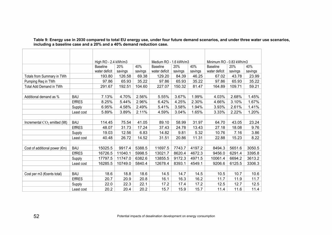
Potential impacts of desalination development on energy consumption 52
Table 9: Energy use in 2030 compared to total EU energy use, under four future demand scenarios, and under three water use scenarios, including a baseline case and a 20% and a 40% demand reduction case.
High RO - 2.4 kWh/m3 Medium RO - 1.6 kWh/m3 Minimum RO - 0.83 kWh/m3
Baseline water deficit
20% savings
40% savings
Baseline water deficit
20% savings
40% savings
Baseline water deficit
20% savings
40% savings
Totals from Summary in TWh 193.80 126.58 69.38 129.20 84.39 46.25 67.02 43.78 23.99Pumping Req in TWh 97.86 65.93 35.22 97.86 65.93 35.22 97.86 65.93 35.22Total Add Demand in TWh 291.67 192.51 104.60 227.07 150.32 81.47 164.89 109.71 59.21 Additional demand as % BAU 7.13% 4.70% 2.56% 5.55% 3.67% 1.99% 4.03% 2.68% 1.45% EffRES 8.25% 5.44% 2.96% 6.42% 4.25% 2.30% 4.66% 3.10% 1.67% Supply 6.95% 4.58% 2.49% 5.41% 3.58% 1.94% 3.93% 2.61% 1.41% Least cost 5.89% 3.89% 2.11% 4.59% 3.04% 1.65% 3.33% 2.22% 1.20% Incremental CO2 emitted (Mt) BAU 114.45 75.54 41.05 89.10 58.99 31.97 64.70 43.05 23.24 EffRES 48.07 31.73 17.24 37.43 24.78 13.43 27.18 18.08 9.76 Supply 19.03 12.56 6.83 14.82 9.81 5.32 10.76 7.16 3.86 Least cost 40.48 26.72 14.52 31.51 20.86 11.31 22.88 15.23 8.22 Cost of additional power (€m) BAU 15025.5 9917.4 5388.5 11697.5 7743.7 4197.2 8494.3 5651.6 3050.5 EffRES 16726.5 11040.1 5998.5 13021.7 8620.4 4672.3 9456.0 6291.4 3395.8 Supply 17797.5 11747.0 6382.6 13855.5 9172.3 4971.5 10061.4 6694.2 3613.2 Least cost 16285.5 10749.0 5840.4 12678.4 8393.1 4549.1 9206.6 6125.5 3306.3 Cost per m3 (€cents total) BAU 18.6 18.8 18.6 14.5 14.7 14.5 10.5 10.7 10.6 EffRES 20.7 20.9 20.8 16.1 16.3 16.2 11.7 11.9 11.7 Supply 22.0 22.3 22.1 17.2 17.4 17.2 12.5 12.7 12.5 Least cost 20.2 20.4 20.2 15.7 15.9 15.7 11.4 11.6 11.4
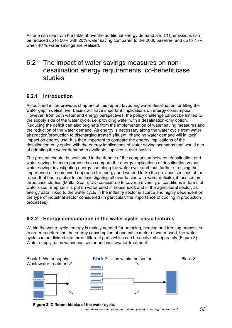
Potential impacts of desalination development on energy consumption 53
As one can see from the table above the additional energy demand and CO2 emissions can be reduced up to 50% with 20% water saving compared to the 2030 baseline, and up to 75% when 40 % water savings are realised.
6.2 The impact of water savings measures on non-desalination energy requirements: co-benefit case studies
6.2.1 Introduction
As outlined in the previous chapters of this report, favouring water desalination for filling the water gap in deficit river basins will have important implications on energy consumption. However, from both water and energy perspectives, the policy challenge cannot be limited to the supply side of the water cycle, i.e. providing water with a desalination-only option. Reducing the deficit can also originate from the implementation of water saving measures and the reduction of the water demand. As energy is necessary along the water cycle from water abstraction/production to discharging treated effluent, changing water demand will in itself impact on energy use. It is then important to compare the energy implications of the desalination-only option with the energy implications of water saving scenarios that would aim at adapting the water demand to available supplies in river basins.
The present chapter is positioned in the debate of the comparison between desalination and water saving. Its main purpose is to compare the energy implications of desalination versus water saving, investigating energy use along the water cycle and thus further stressing the importance of a combined approach for energy and water. Unlike the previous sections of the report that had a global focus (investigating all river basins with water deficits), it focuses on three case studies (Malta, Spain, UK) considered to cover a diversity of conditions in terms of water uses. Emphasis is put on water used in households and in the agricultural sector, as energy data linked to the water cycle in the industry sector is scarce and highly dependent on the type of industrial sector considered (in particular, the importance of cooling in production processes).
6.2.2 Energy consumption in the water cycle: basic features
Within the water cycle, energy is mainly needed for pumping, heating and treating processes. In order to determine the energy consumption of one cubic meter of water used, the water cycle can be divided into three different parts which can be analyzed separately (Figure 3): Water supply, uses within one sector and wastewater treatment.
Block 1: Water supply Block 2: Uses within the sector Block 3: Wastewater treatment
Figure 3: Different blocks of the water cycle.
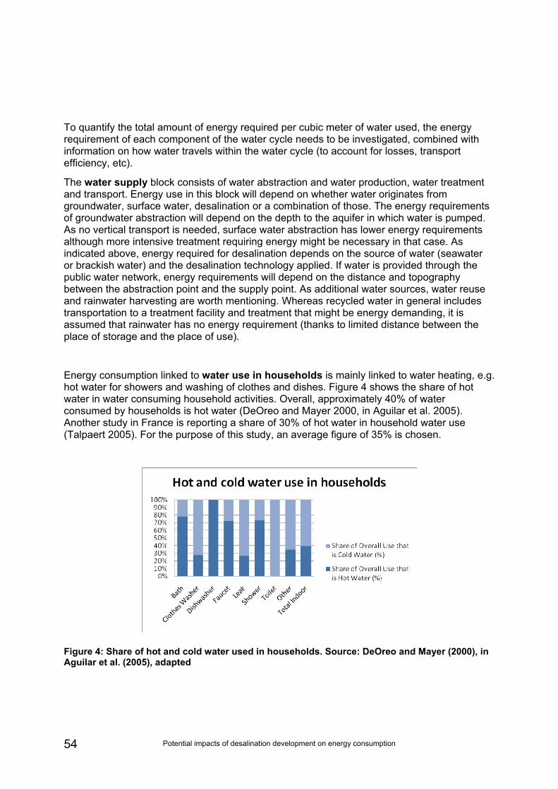
Potential impacts of desalination development on energy consumption 54
To quantify the total amount of energy required per cubic meter of water used, the energy requirement of each component of the water cycle needs to be investigated, combined with information on how water travels within the water cycle (to account for losses, transport efficiency, etc).
The water supply block consists of water abstraction and water production, water treatment and transport. Energy use in this block will depend on whether water originates from groundwater, surface water, desalination or a combination of those. The energy requirements of groundwater abstraction will depend on the depth to the aquifer in which water is pumped. As no vertical transport is needed, surface water abstraction has lower energy requirements although more intensive treatment requiring energy might be necessary in that case. As indicated above, energy required for desalination depends on the source of water (seawater or brackish water) and the desalination technology applied. If water is provided through the public water network, energy requirements will depend on the distance and topography between the abstraction point and the supply point. As additional water sources, water reuse and rainwater harvesting are worth mentioning. Whereas recycled water in general includes transportation to a treatment facility and treatment that might be energy demanding, it is assumed that rainwater has no energy requirement (thanks to limited distance between the place of storage and the place of use).
Energy consumption linked to water use in households is mainly linked to water heating, e.g. hot water for showers and washing of clothes and dishes. Figure 4 shows the share of hot water in water consuming household activities. Overall, approximately 40% of water consumed by households is hot water (DeOreo and Mayer 2000, in Aguilar et al. 2005). Another study in France is reporting a share of 30% of hot water in household water use (Talpaert 2005). For the purpose of this study, an average figure of 35% is chosen.
Figure 4: Share of hot and cold water used in households. Source: DeOreo and Mayer (2000), in Aguilar et al. (2005), adapted
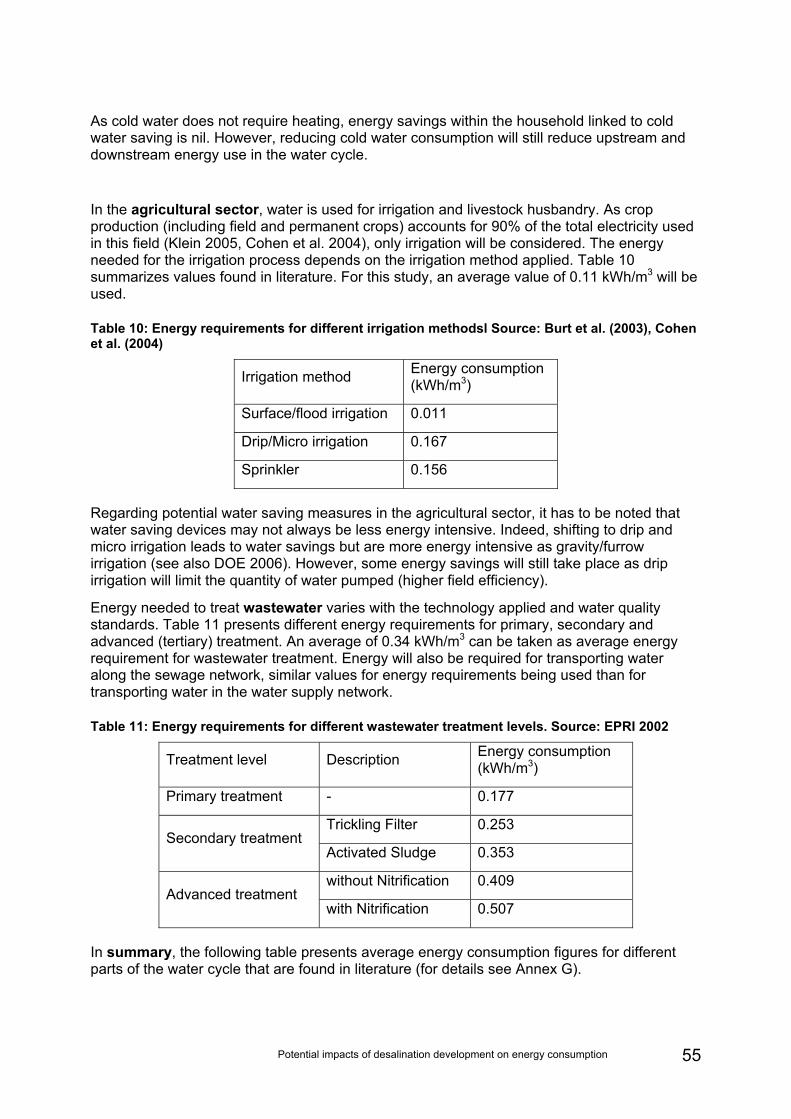
Potential impacts of desalination development on energy consumption 55
As cold water does not require heating, energy savings within the household linked to cold water saving is nil. However, reducing cold water consumption will still reduce upstream and downstream energy use in the water cycle.
In the agricultural sector, water is used for irrigation and livestock husbandry. As crop production (including field and permanent crops) accounts for 90% of the total electricity used in this field (Klein 2005, Cohen et al. 2004), only irrigation will be considered. The energy needed for the irrigation process depends on the irrigation method applied. Table 10 summarizes values found in literature. For this study, an average value of 0.11 kWh/m3 will be used.
Table 10: Energy requirements for different irrigation methodsl Source: Burt et al. (2003), Cohen et al. (2004)
Irrigation method Energy consumption (kWh/m3)
Surface/flood irrigation 0.011
Drip/Micro irrigation 0.167
Sprinkler 0.156
Regarding potential water saving measures in the agricultural sector, it has to be noted that water saving devices may not always be less energy intensive. Indeed, shifting to drip and micro irrigation leads to water savings but are more energy intensive as gravity/furrow irrigation (see also DOE 2006). However, some energy savings will still take place as drip irrigation will limit the quantity of water pumped (higher field efficiency).
Energy needed to treat wastewater varies with the technology applied and water quality standards. Table 11 presents different energy requirements for primary, secondary and advanced (tertiary) treatment. An average of 0.34 kWh/m3 can be taken as average energy requirement for wastewater treatment. Energy will also be required for transporting water along the sewage network, similar values for energy requirements being used than for transporting water in the water supply network.
Table 11: Energy requirements for different wastewater treatment levels. Source: EPRI 2002
Treatment level Description Energy consumption (kWh/m3)
Primary treatment - 0.177
Trickling Filter 0.253 Secondary treatment
Activated Sludge 0.353
without Nitrification 0.409 Advanced treatment
with Nitrification 0.507
In summary, the following table presents average energy consumption figures for different parts of the water cycle that are found in literature (for details see Annex G).
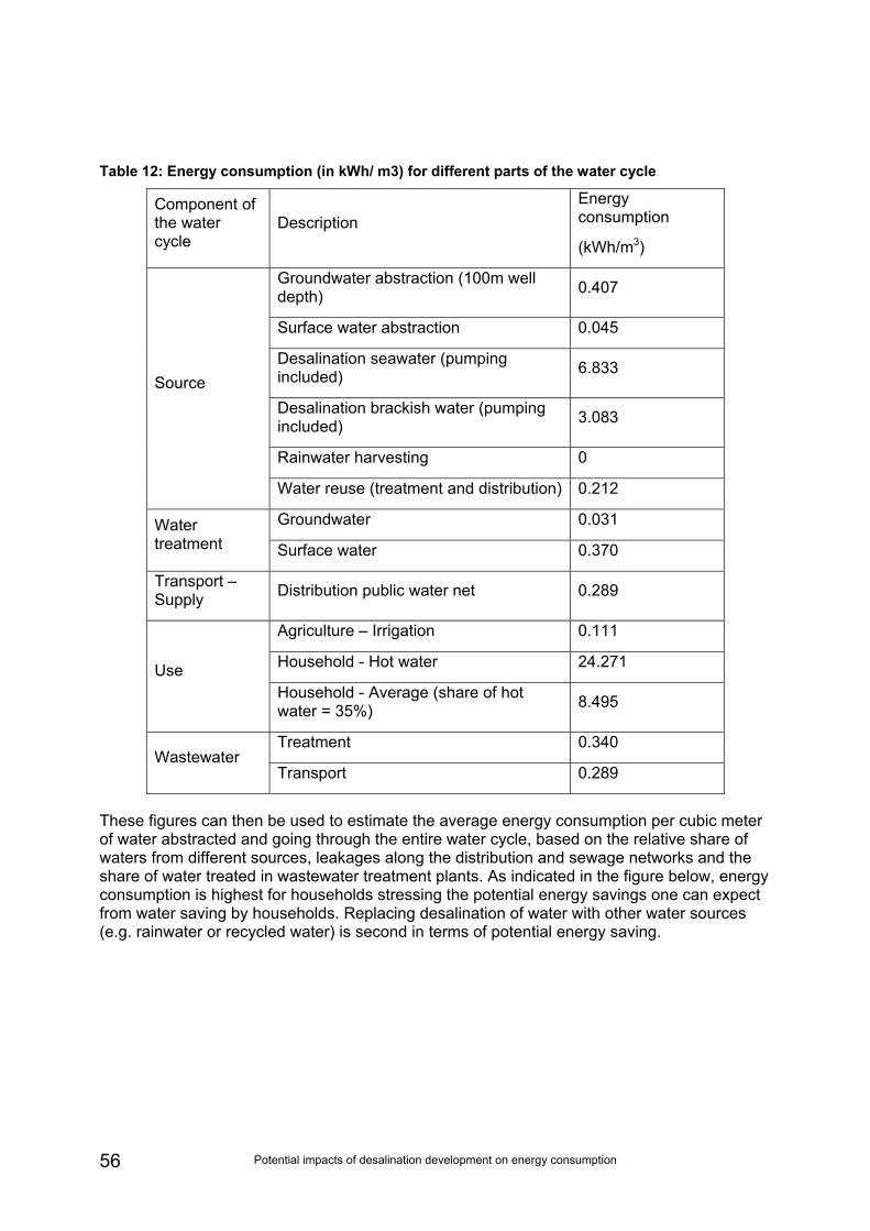
Potential impacts of desalination development on energy consumption 56
Table 12: Energy consumption (in kWh/ m3) for different parts of the water cycle
Component of the water cycle
Description Energy consumption
(kWh/m3)
Groundwater abstraction (100m well depth) 0.407
Surface water abstraction 0.045
Desalination seawater (pumping included) 6.833
Desalination brackish water (pumping included) 3.083
Rainwater harvesting 0
Source
Water reuse (treatment and distribution) 0.212
Groundwater 0.031 Water treatment Surface water 0.370
Transport – Supply Distribution public water net 0.289
Agriculture – Irrigation 0.111
Household - Hot water 24.271 Use Household - Average (share of hot water = 35%) 8.495
Treatment 0.340 Wastewater
Transport 0.289
These figures can then be used to estimate the average energy consumption per cubic meter of water abstracted and going through the entire water cycle, based on the relative share of waters from different sources, leakages along the distribution and sewage networks and the share of water treated in wastewater treatment plants. As indicated in the figure below, energy consumption is highest for households stressing the potential energy savings one can expect from water saving by households. Replacing desalination of water with other water sources (e.g. rainwater or recycled water) is second in terms of potential energy saving.
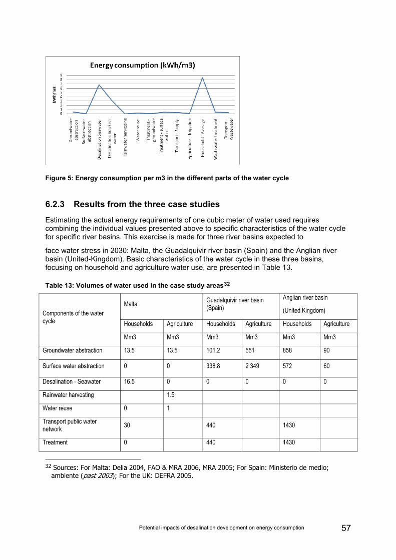
Potential impacts of desalination development on energy consumption 57
Figure 5: Energy consumption per m3 in the different parts of the water cycle
6.2.3 Results from the three case studies
Estimating the actual energy requirements of one cubic meter of water used requires combining the individual values presented above to specific characteristics of the water cycle for specific river basins. This exercise is made for three river basins expected to
face water stress in 2030: Malta, the Guadalquivir river basin (Spain) and the Anglian river basin (United-Kingdom). Basic characteristics of the water cycle in these three basins, focusing on household and agriculture water use, are presented in Table 13.
Table 13: Volumes of water used in the case study areas32
Malta Guadalquivir river basin (Spain)
Anglian river basin
(United Kingdom)
Households Agriculture Households Agriculture Households Agriculture Components of the water cycle
Mm3 Mm3 Mm3 Mm3 Mm3 Mm3
Groundwater abstraction 13.5 13.5 101.2 551 858 90
Surface water abstraction 0 0 338.8 2 349 572 60
Desalination - Seawater 16.5 0 0 0 0 0
Rainwater harvesting 1.5 Water reuse 0 1 Transport public water network 30 440 1430
Treatment 0 440 1430
32 Sources: For Malta: Delia 2004, FAO & MRA 2006, MRA 2005; For Spain: Ministerio de medio;
ambiente (past 2003); For the UK: DEFRA 2005.
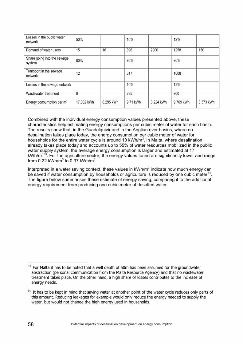
Potential impacts of desalination development on energy consumption 58
Losses in the public water network 50% 10% 12%
Demand of water users 15 16 396 2900 1258 150
Share going into the sewage system 80% 80% 80%
Transport in the sewage network 12 317 1008
Losses in the sewage network 10% 12%
Wastewater treatment 0 285 900 Energy consumption per m3 17.032 kWh 0.295 kWh 9.71 kWh 0.224 kWh 9.769 kWh 0.373 kWh
Combined with the individual energy consumption values presented above, these characteristics help estimating energy consumptions per cubic meter of water for each basin. The results show that, in the Guadalquivir and in the Anglian river basins, where no desalination takes place today, the energy consumption per cubic meter of water for households for the entire water cycle is around 10 kWh/m3. In Malta, where desalination already takes place today and accounts up to 55% of water resources mobilized in the public water supply system, the average energy consumption is larger and estimated at 17 kWh/m333. For the agriculture sector, the energy values found are significantly lower and range from 0.22 kWh/m3 to 0.37 kWh/m3.
Interpreted in a water saving context, these values in kWh/m3 indicate how much energy can be saved if water consumption by households or agriculture is reduced by one cubic meter34. The figure below summarises these estimate of energy saving, comparing it to the additional energy requirement from producing one cubic meter of desalted water.
33 For Malta it has to be noted that a well depth of 50m has been assumed for the groundwater
abstraction (personal communication from the Malta Resource Agency) and that no wastewater treatment takes place. On the other hand, a high share of losses contributes to the increase of energy needs.
34 It has to be kept in mind that saving water at another point of the water cycle reduces only parts of this amount. Reducing leakages for example would only reduce the energy needed to supply the water, but would not change the high energy used in households.
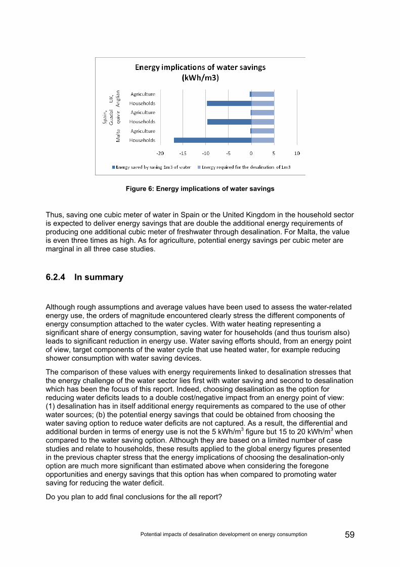
Potential impacts of desalination development on energy consumption 59
Figure 6: Energy implications of water savings
Thus, saving one cubic meter of water in Spain or the United Kingdom in the household sector is expected to deliver energy savings that are double the additional energy requirements of producing one additional cubic meter of freshwater through desalination. For Malta, the value is even three times as high. As for agriculture, potential energy savings per cubic meter are marginal in all three case studies.
6.2.4 In summary
Although rough assumptions and average values have been used to assess the water-related energy use, the orders of magnitude encountered clearly stress the different components of energy consumption attached to the water cycles. With water heating representing a significant share of energy consumption, saving water for households (and thus tourism also) leads to significant reduction in energy use. Water saving efforts should, from an energy point of view, target components of the water cycle that use heated water, for example reducing shower consumption with water saving devices.
The comparison of these values with energy requirements linked to desalination stresses that the energy challenge of the water sector lies first with water saving and second to desalination which has been the focus of this report. Indeed, choosing desalination as the option for reducing water deficits leads to a double cost/negative impact from an energy point of view: (1) desalination has in itself additional energy requirements as compared to the use of other water sources; (b) the potential energy savings that could be obtained from choosing the water saving option to reduce water deficits are not captured. As a result, the differential and additional burden in terms of energy use is not the 5 kWh/m3 figure but 15 to 20 kWh/m3 when compared to the water saving option. Although they are based on a limited number of case studies and relate to households, these results applied to the global energy figures presented in the previous chapter stress that the energy implications of choosing the desalination-only option are much more significant than estimated above when considering the foregone opportunities and energy savings that this option has when compared to promoting water saving for reducing the water deficit.
Do you plan to add final conclusions for the all report?
Potential impacts of desalination development on energy consumption 60
7 References
Aguilar. C.. White. D.J. and Ryan. D.L. (2005) ‘Domestic Water Heating and Water Heater Energy Consumption in Canada’. CBEEDAC 2005-RP-02. Canada. http://www.ualberta.ca/~cbeedac/publications/documents/domwater_000.pdf
Burt, C.; Howes, D. and Wilson, G. (2003) ‘California Agricultural Water Electrical Energy Requirements’, ITRC Report No. R 03-006, http://www.itrc.org/reports/energyreq/energyreq.pdf
Cohen, R., Nelson, B. and Wolff, G. (2004) ‘Energy down the drain. The Hidden Costs of California’s Water Supply’; NRDC and Pacific Institute; http://www.nrdc.org/water/conservation/edrain/contents.asp
DEFRA (2005), 'WFD Summary report of the characterisation, impacts and economics analyses required by Article 5, Anglian river basin district', March 2005
Delia C. (2004), 'Economic considerations regarding markets for water in the Maltese islands'
DOE (U.S. Department of Energy) (2006) ‘Energy demands on water resources’, Report to Congress on the interdependency of energy and water; http://www.sandia.gov/energy-water/docs/121-RptToCongress-EWwEIAcomments-FINAL.pdf
EPRI (Electric Power Research Institute) (2002) ‘Water & Sustainability (Volume 4): U.S. Electricity Consumption for Water Supply & Treatment – The Next Half Century’, 1006787, Palo Alto, California
FAO (Food and Agriculture Organisation) and MRA (Maltese Resources Authority) (2006), 'Malta water ressource review'
Flörke, M.; Alcamo, J. (2004): European Outlook on Water Use, Final Report, 1 October 2004.
Klein, G. (2005) ‘California’s Water – Energy Relationship’, California Energy Commission, Prepared in Support of the 2005 Integrated Energy Policy Report Proceeding
Mantzos, L. and P. Capros (2005): European Energy and Transport Trends to 2030, update 2005. for the European Commission, Directorate General for Energy and Transport.
Ministerio de medio ambiante, Confederacion Hidrografica del Guadalquivir (past 2003) 'WFD Article 5: Analisis economico, Guadalquivir'
MRA (Maltese Resources Authority) (2005), 'Water Framework Directive Article 5: Reporting sheets', March 2005
Talpaert, L. (2005) 'Inventaire des materiels hydro-economies', CREAQ, Bordeaux
Potential impacts of desalination development on energy consumption 61
Annex A: Method to assess current water prices in river basins The main source used for the water prices is the International Water Association (IWA 2006). Price information is available for different cities in more than 20 countries. As no information is available for Bulgaria, Malta and the UK, different sources have been used for these countries: Bardarska (2004), Malta Resource Authority (2005) and OFWAT (200435), respectively.
In order to obtain the relevant price levels for each River basin affected by water scarcity in 2030, the following method has been applied:
• Linking towns to river basins: To get an idea of the water prices in the affected river basins, it was checked whether one or more of the towns listed in the IWA document are lying in the respective area. If this was the case, the average value out of this data was applied to the basin. If none of the towns corresponded to a river basin, the average value for the country was used. This explains why some values for one country are exactly the same.
• Conversion of the values in €s and calculation of a unitary fixed cost: The figures from IWA were given in US Dollar for the year 2005 and for a consumption of 200 m3. Therefore the values have been converted to € (applied conversion factor: 1 US Dollar = 0.82898 €36) and divided by 200, in order to get data for 1 m3. Only the value for the fixed charge was divided by the average household consumption per year in the respective country to get a rough estimation of the value per cubic meter.
However it is important to highlight the limits of the method. As mentioned before, it was not possible to find corresponding cities for all the river basins. So no real regional price information could be derived in these cases. Considering as well the regional variability and the fact that sometimes the water price taken for one basin is only based on one city within it, the results have to be treated with great care. To solve this problem, a more detailed set of data would be needed. Furthermore, as different sources had to be used for some countries, not all the figures listed have been collected and calculated in the same manner.
Checking the data with other sources
Accounting for the problems mentioned before, it was proposed to check price information taken from IWA with other sources of information. One possible way was be to look at the Article 5 reports, which EU Member States had to deliver in the course of the Water Framework Directive and which should also include economic information for the respective river basins. An example is given for the Jucar river basin, Spain (Estrela et al. 2004). For Denmark, other national figures could be found.
35 Data for the average yearly household bills were divided by the average household consumption of
127m3. 36 Source: www.umrechnung24.de; 30.6.2005
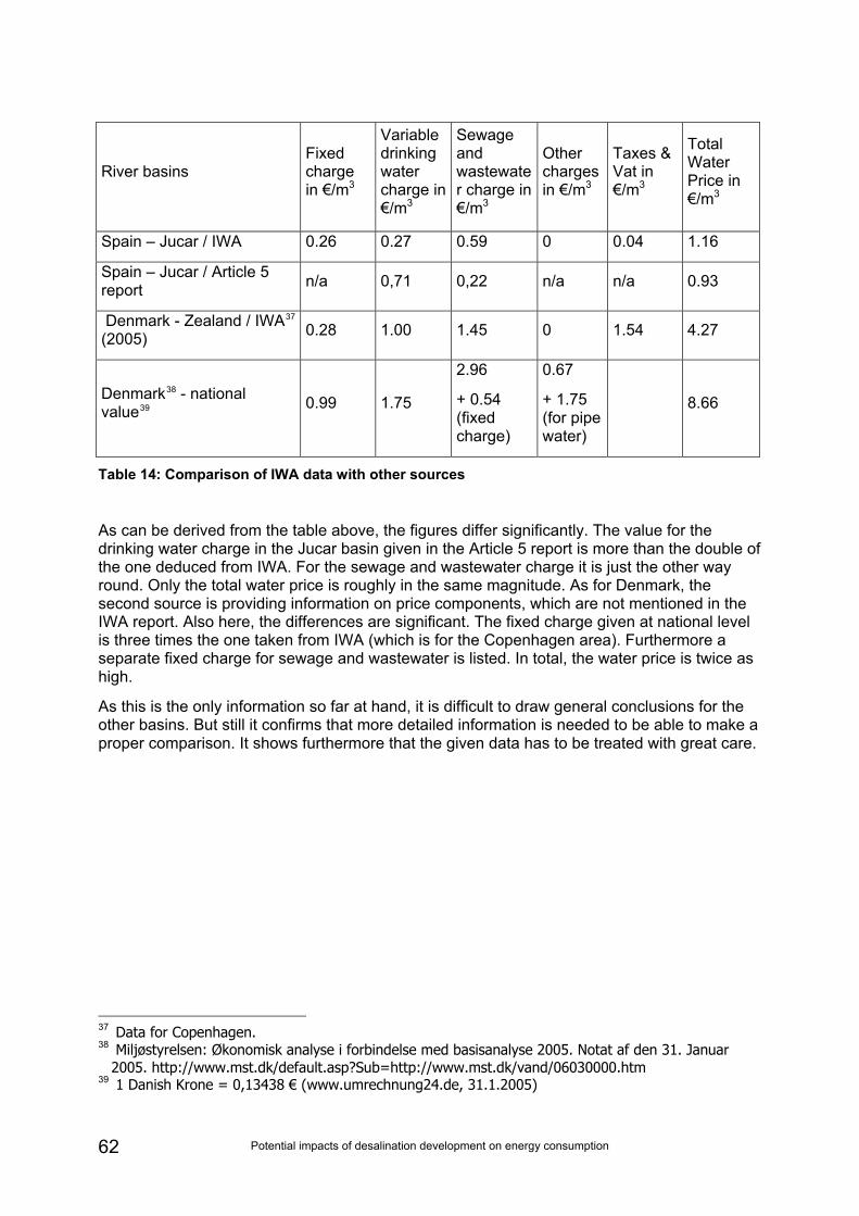
Potential impacts of desalination development on energy consumption 62
River basins Fixed charge in €/m3
Variable drinking water charge in €/m3
Sewage and wastewater charge in €/m3
Other charges in €/m3
Taxes & Vat in €/m3
Total Water Price in €/m3
Spain – Jucar / IWA 0.26 0.27 0.59 0 0.04 1.16
Spain – Jucar / Article 5 report n/a 0,71 0,22 n/a n/a 0.93
Denmark - Zealand / IWA37 (2005) 0.28 1.00 1.45 0 1.54 4.27
Denmark38 - national value39 0.99 1.75
2.96
+ 0.54 (fixed charge)
0.67
+ 1.75 (for pipe water)
8.66
Table 14: Comparison of IWA data with other sources
As can be derived from the table above, the figures differ significantly. The value for the drinking water charge in the Jucar basin given in the Article 5 report is more than the double of the one deduced from IWA. For the sewage and wastewater charge it is just the other way round. Only the total water price is roughly in the same magnitude. As for Denmark, the second source is providing information on price components, which are not mentioned in the IWA report. Also here, the differences are significant. The fixed charge given at national level is three times the one taken from IWA (which is for the Copenhagen area). Furthermore a separate fixed charge for sewage and wastewater is listed. In total, the water price is twice as high.
As this is the only information so far at hand, it is difficult to draw general conclusions for the other basins. But still it confirms that more detailed information is needed to be able to make a proper comparison. It shows furthermore that the given data has to be treated with great care.
37 Data for Copenhagen. 38 Miljøstyrelsen: Økonomisk analyse i forbindelse med basisanalyse 2005. Notat af den 31. Januar
2005. http://www.mst.dk/default.asp?Sub=http://www.mst.dk/vand/06030000.htm 39 1 Danish Krone = 0,13438 € (www.umrechnung24.de, 31.1.2005)
Potential impacts of desalination development on energy consumption 63
Annex B: Method for estimating future “baseline” water prices As estimating developments in the future is always difficult and the level of detail possible in this part of the study is clearly limiting, a simple rule has to be found which enables to make rough assumptions on the weight of each directive in the future water prices. The directives considered are:
The Urban Wasterwater Treatment Directives
The Drinking Water Directive
The Water Framework Directive, especially article 9: cost recovery
One way would be to look at the planned investments in every country and to try to convert them into prices per cubic meter. Another possibility is to apply values found for those countries which are already fulfilling the requirements of the directive – as for example the Netherlands and Denmark for UWWTD – to the rest of the EU member states. The first method would require looking at the planned investments, the level of implementation today and the current level of cost recovery through consumer prices. This section aims at choosing the right method to evaluate the additional cost linked to the implementation of each directive in the future water price.
Constraints to the estimation
Besides the general difficulties to predict future developments, it has to be kept in mind that the relevant information for the water prices is needed at river basin level, whereas the available figures are only given for the national level. This means that it cannot not be taken into account that some river basins might already have implemented all the necessary facilities and do not need any further investments in this regard.
Urban Wastewater Treatment Directive The methods described below in order to take the influence of the UWWTD into account are mainly derived from the situations in those countries which are (nearly) fully complying with the UWWTD requirements. They relate to the percentage of GDP spent for wastewater treatment, to costs per capita and per cubic meter or to the existing ratio between drinking water and wastewater charges.
Method 1: Water treatment expenditures as a share of GDP
In the Netherlands the average annual expenditures for water pollution control measures account for 0.05% of the national GDP. This is less than in Spain (0.12%) and France (0.06%) although the last two countries are not yet fully complying with the directive. According to EEA (2005), this would be due to the cost effectiveness of the measures implemented in the Netherlands. Also Denmark – as a country which as well meets the requirements – implemented rather costly measures as the expenditures for water treatment account there for a yearly percentage of 0.17% of the GDP (EEA 2005).
For this study, the assumption could be made that cost-effectiveness in the water sector will increase and that the situation in the Netherlands can be used as a point of reference for the
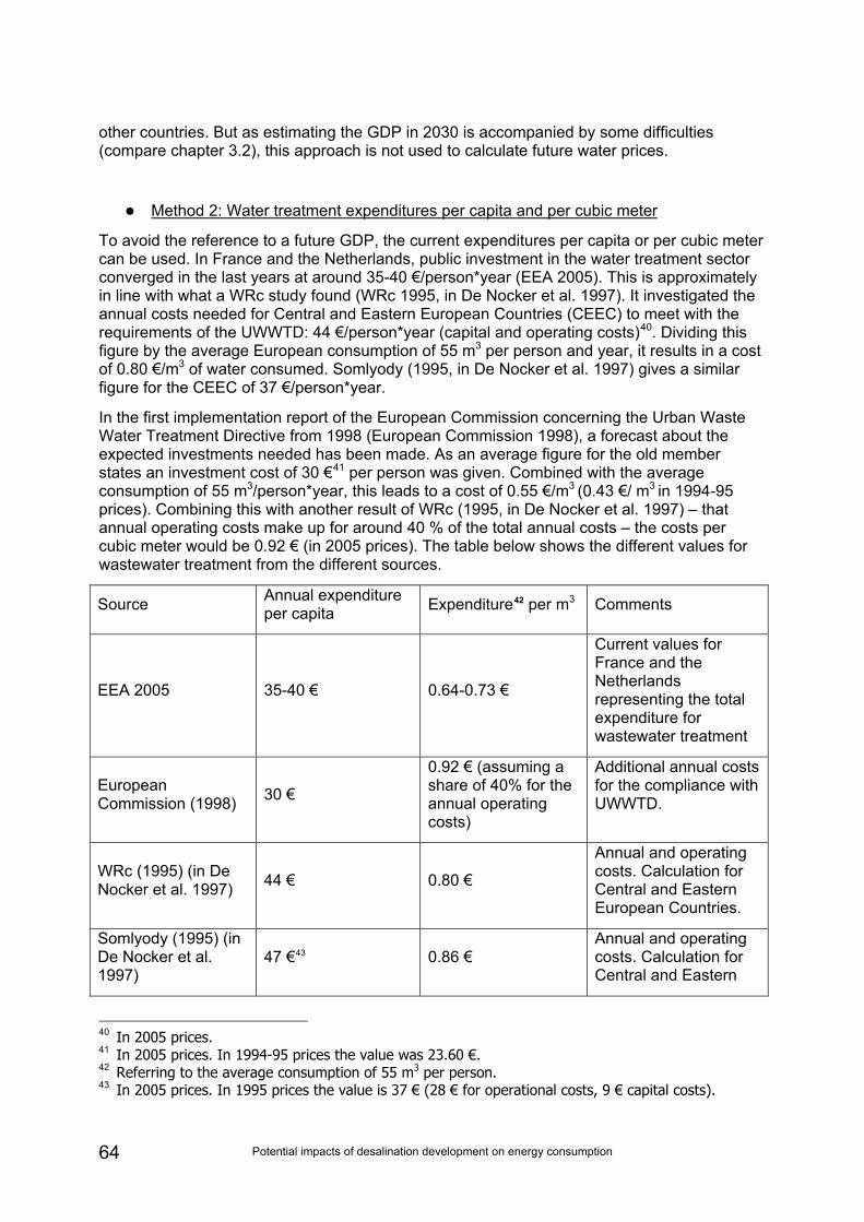
Potential impacts of desalination development on energy consumption 64
other countries. But as estimating the GDP in 2030 is accompanied by some difficulties (compare chapter 3.2), this approach is not used to calculate future water prices.
Method 2: Water treatment expenditures per capita and per cubic meter
To avoid the reference to a future GDP, the current expenditures per capita or per cubic meter can be used. In France and the Netherlands, public investment in the water treatment sector converged in the last years at around 35-40 €/person*year (EEA 2005). This is approximately in line with what a WRc study found (WRc 1995, in De Nocker et al. 1997). It investigated the annual costs needed for Central and Eastern European Countries (CEEC) to meet with the requirements of the UWWTD: 44 €/person*year (capital and operating costs)40. Dividing this figure by the average European consumption of 55 m3 per person and year, it results in a cost of 0.80 €/m3 of water consumed. Somlyody (1995, in De Nocker et al. 1997) gives a similar figure for the CEEC of 37 €/person*year.
In the first implementation report of the European Commission concerning the Urban Waste Water Treatment Directive from 1998 (European Commission 1998), a forecast about the expected investments needed has been made. As an average figure for the old member states an investment cost of 30 €41 per person was given. Combined with the average consumption of 55 m3/person*year, this leads to a cost of 0.55 €/m3 (0.43 €/ m3 in 1994-95 prices). Combining this with another result of WRc (1995, in De Nocker et al. 1997) – that annual operating costs make up for around 40 % of the total annual costs – the costs per cubic meter would be 0.92 € (in 2005 prices). The table below shows the different values for wastewater treatment from the different sources.
Source Annual expenditure per capita Expenditure42 per m3 Comments
EEA 2005 35-40 € 0.64-0.73 €
Current values for France and the Netherlands representing the total expenditure for wastewater treatment
European Commission (1998) 30 €
0.92 € (assuming a share of 40% for the annual operating costs)
Additional annual costs for the compliance with UWWTD.
WRc (1995) (in De Nocker et al. 1997) 44 € 0.80 €
Annual and operating costs. Calculation for Central and Eastern European Countries.
Somlyody (1995) (in De Nocker et al. 1997)
47 €43 0.86 € Annual and operating costs. Calculation for Central and Eastern
40 In 2005 prices. 41 In 2005 prices. In 1994-95 prices the value was 23.60 €. 42 Referring to the average consumption of 55 m3 per person. 43 In 2005 prices. In 1995 prices the value is 37 € (28 € for operational costs, 9 € capital costs).
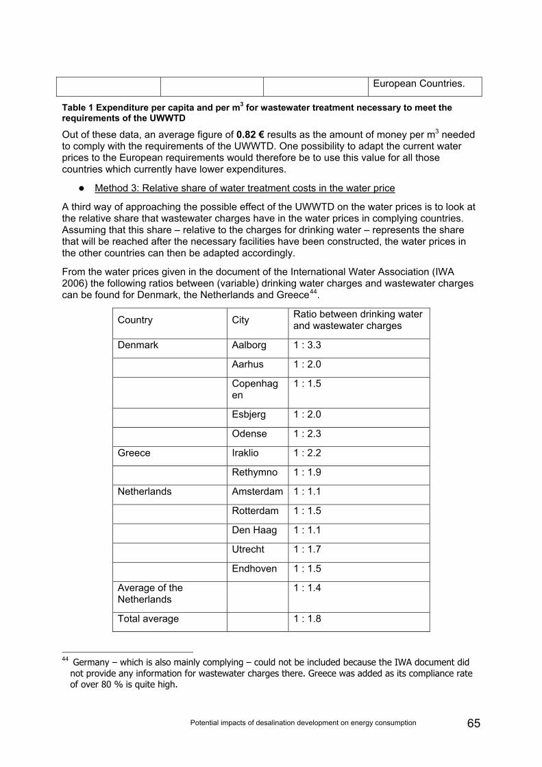
Potential impacts of desalination development on energy consumption 65
European Countries.
Table 1 Expenditure per capita and per m3 for wastewater treatment necessary to meet the requirements of the UWWTD
Out of these data, an average figure of 0.82 € results as the amount of money per m3 needed to comply with the requirements of the UWWTD. One possibility to adapt the current water prices to the European requirements would therefore be to use this value for all those countries which currently have lower expenditures.
Method 3: Relative share of water treatment costs in the water price
A third way of approaching the possible effect of the UWWTD on the water prices is to look at the relative share that wastewater charges have in the water prices in complying countries. Assuming that this share – relative to the charges for drinking water – represents the share that will be reached after the necessary facilities have been constructed, the water prices in the other countries can then be adapted accordingly.
From the water prices given in the document of the International Water Association (IWA 2006) the following ratios between (variable) drinking water charges and wastewater charges can be found for Denmark, the Netherlands and Greece44.
Country City Ratio between drinking water and wastewater charges
Denmark Aalborg 1 : 3.3
Aarhus 1 : 2.0
Copenhagen
1 : 1.5
Esbjerg 1 : 2.0
Odense 1 : 2.3
Greece Iraklio 1 : 2.2
Rethymno 1 : 1.9
Netherlands Amsterdam 1 : 1.1
Rotterdam 1 : 1.5
Den Haag 1 : 1.1
Utrecht 1 : 1.7
Endhoven 1 : 1.5
Average of the Netherlands
1 : 1.4
Total average 1 : 1.8
44 Germany – which is also mainly complying – could not be included because the IWA document did
not provide any information for wastewater charges there. Greece was added as its compliance rate of over 80 % is quite high.
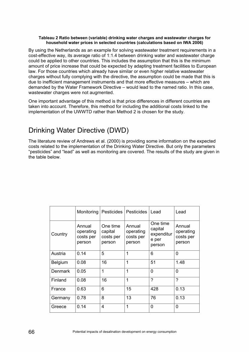
Potential impacts of desalination development on energy consumption 66
Tableau 2 Ratio between (variable) drinking water charges and wastewater charges for household water prices in selected countries (calculations based on IWA 2006)
By using the Netherlands as an example for solving wastewater treatment requirements in a cost-effective way, its average ratio of 1:1.4 between drinking water and wastewater charge could be applied to other countries. This includes the assumption that this is the minimum amount of price increase that could be expected by adapting treatment facilities to European law. For those countries which already have similar or even higher relative wastewater charges without fully complying with the directive, the assumption could be made that this is due to inefficient management instruments and that more effective measures – which are demanded by the Water Framework Directive – would lead to the named ratio. In this case, wastewater charges were not augmented.
One important advantage of this method is that price differences in different countries are taken into account. Therefore, this method for including the additional costs linked to the implementation of the UWWTD rather than Method 2 is chosen for the study.
Drinking Water Directive (DWD) The literature review of Andrews et al. (2000) is providing some information on the expected costs related to the implementation of the Drinking Water Directive. But only the parameters “pesticides” and “lead” as well as monitoring are covered. The results of the study are given in the table below.
Monitoring Pesticides Pesticides Lead Lead
Country
Annual operating costs per person
One time capital costs per person
Annual operating costs per person
One time capital expenditure per person
Annual operating costs per person
Austria 0.14 5 1 6 0
Belgium 0.08 16 1 51 1.48
Denmark 0.05 1 1 0 0
Finland 0.08 16 1 ? ?
France 0.63 6 15 428 0.13
Germany 0.78 8 13 76 0.13
Greece 0.14 4 1 0 0
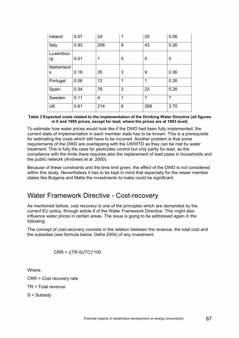
Potential impacts of desalination development on energy consumption 67
Ireland 0.07 24 1 25 0.06
Italy 0.93 206 9 43 0.26
Luxembourg 0.01 1 0 0 0
Netherlands 0.18 35 3 9 0.36
Portugal 0.06 12 1 1 0.26
Spain 0.34 76 3 23 0.26
Sweden 0.11 4 1 ? ?
UK 0.61 214 6 268 3.70
Table 3 Expected costs related to the implementation of the Drinking Water Directive (all figures in € and 1995 prices, except for lead, where the prices are at 1993 level)
To estimate how water prices would look like if the DWD had been fully implemented, the current state of implementation in each member state has to be known. This is a prerequisite for estimating the costs which still have to be incurred. Another problem is that some requirements of the DWD are overlapping with the UWWTD as they can be met by water treatment. This is fully the case for pesticides control but only partly for lead, as the compliance with the limits there requires also the replacement of lead pipes in households and the public network (Andrews et al. 2000).
Because of these constraints and the time limit given, the effect of the DWD is not considered within this study. Nevertheless it has to be kept in mind that especially for the newer member states like Bulgaria and Malta the investments to make could be significant.
Water Framework Directive - Cost-recovery As mentioned before, cost recovery is one of the principles which are demanded by the current EU policy, through article 9 of the Water Framework Directive. This might also influence water prices in certain areas. The issue is going to be addressed again in the following.
The concept of cost-recovery consists in the relation between the revenue, the total cost and the subsidies (see formula below; Defra 2004) of any investment.
CRR = ((TR-S)/TC)*100
Where,
CRR = Cost recovery rate
TR = Total revenue
S = Subsidy
Potential impacts of desalination development on energy consumption 68
TC = Total cost
However, there is no universal definition of the concept, as each definition depends on the nature of the cost considered (costs concerning operating and maintenance, capital, opportunity costs, resources, social costs, environmental damage, etc) and none of them is really completed (Roth 2001). Despite that problem, some figures found in literature are given in the following. The most accurate data is given for Cyprus in 2005. Indeed, the calculation has been made for domestic water supply – including and excluding environmental costs. When not included, the level of cost-recovery is 73%. In the second case, the level accounts for 62%45.
In England and Wales, according to DEFRA (2004), the cost-recovery rate for public water supply and sewerage services has reached 100% since 1998.
Also a study about countries from the CIS region (former USSR region) has been found (Maslyukivska (n/a)). The cost recovery rate ranges from 55% to 90% in 2005. This gives an idea of the level of cost-recovery in the countries close to eastern €pe.
Another study for northern European countries revealed that the level of cost-recovery for water supply and sewerage is 100% for Denmark, Finland, Latvia, Lithuania, Poland and Sweden46.
Finally, a study from EU Commission – based on information provided by member states on water pricing policies – mentioned a few figures. The fact that only a few figures are given shows that cost-recovery values are in general not well-known (officially) by the member states. In this study, data are provided for France (85% for households and industry, includes environmental charges), Cyprus (73%) and Lithuania (from 74% to 83% depending on the river basin).
Complete data for the basins of interest in the study were not found. However, looking at the previously mentioned data, one can see that all the river basins have now a level of cost-recovery that ranges between 70% and 100% (see also European Commission 2007b). The level would depend on the basin but also on the way to calculate the cost-recovery, i.e. depending on the costs included, as highlighted previously.
In conclusion, it will be assumed that the level of cost-recovery – a few exceptions put aside – will slightly increase the future water prices as compared to other factors (implementation of UWWTD, DWD....). Still, due to a lack of information for all the river basins, this will not be further considered.
45 http://www.planbleu.org/publications/atelier_eau_saragosse/Synthese_rapport_Chypre_EN.pdf 46
http://sea.helcom.fi/dps/docs/documents/Programme%20Implementation%20Task%20Force%20(PITF)/
PITF%2019%20(2002)/5.5-1.pdf
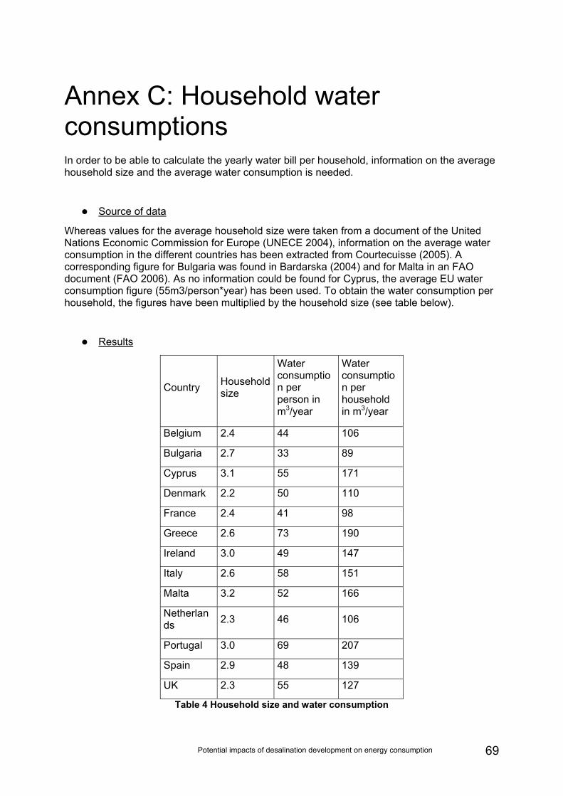
Potential impacts of desalination development on energy consumption 69
Annex C: Household water consumptions In order to be able to calculate the yearly water bill per household, information on the average household size and the average water consumption is needed.
Source of data
Whereas values for the average household size were taken from a document of the United Nations Economic Commission for Europe (UNECE 2004), information on the average water consumption in the different countries has been extracted from Courtecuisse (2005). A corresponding figure for Bulgaria was found in Bardarska (2004) and for Malta in an FAO document (FAO 2006). As no information could be found for Cyprus, the average EU water consumption figure (55m3/person*year) has been used. To obtain the water consumption per household, the figures have been multiplied by the household size (see table below).
Results
Country Household size
Water consumption per person in m3/year
Water consumption per household in m3/year
Belgium 2.4 44 106
Bulgaria 2.7 33 89
Cyprus 3.1 55 171
Denmark 2.2 50 110
France 2.4 41 98
Greece 2.6 73 190
Ireland 3.0 49 147
Italy 2.6 58 151
Malta 3.2 52 166
Netherlands 2.3 46 106
Portugal 3.0 69 207
Spain 2.9 48 139
UK 2.3 55 127
Table 4 Household size and water consumption
Potential impacts of desalination development on energy consumption 70
The highest water consumption per person could be found for Greece (73 m3/year), followed by Portugal with 69 m3/year. Regarding the consumption per household, the order changes and Portugal shows the highest water use with 207 m3/year, followed by Greece with 190 m3/year. The lowest water consumption takes place in Bulgaria (33 m3/person; 89 m3/ household), followed by France (41 m3/person; 98 m3/household).
The assumption is made that the household size and the water consumption do not change in the future. Although this is rather improbable, due to the lack of information no adjustments are made in this regard.
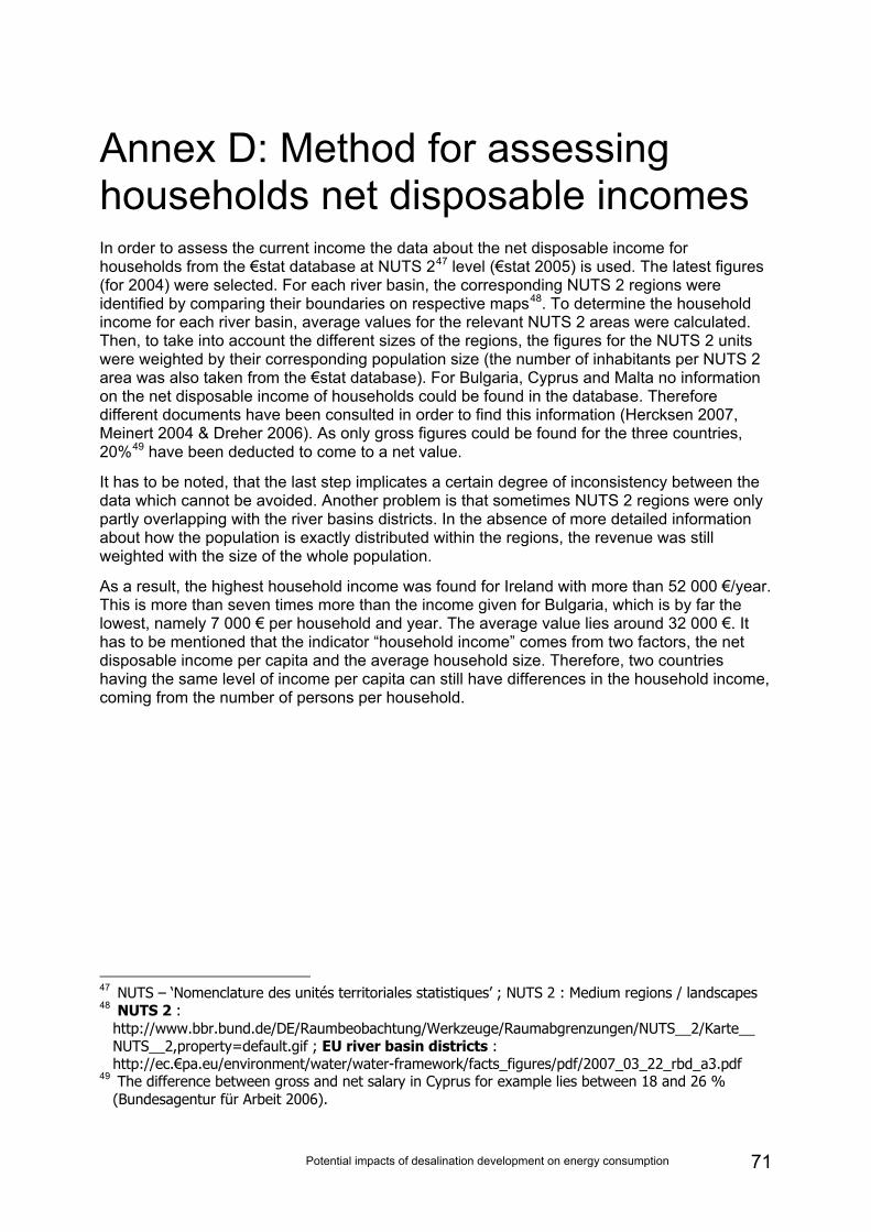
Potential impacts of desalination development on energy consumption 71
Annex D: Method for assessing households net disposable incomes In order to assess the current income the data about the net disposable income for households from the €stat database at NUTS 247 level (€stat 2005) is used. The latest figures (for 2004) were selected. For each river basin, the corresponding NUTS 2 regions were identified by comparing their boundaries on respective maps48. To determine the household income for each river basin, average values for the relevant NUTS 2 areas were calculated. Then, to take into account the different sizes of the regions, the figures for the NUTS 2 units were weighted by their corresponding population size (the number of inhabitants per NUTS 2 area was also taken from the €stat database). For Bulgaria, Cyprus and Malta no information on the net disposable income of households could be found in the database. Therefore different documents have been consulted in order to find this information (Hercksen 2007, Meinert 2004 & Dreher 2006). As only gross figures could be found for the three countries, 20%49 have been deducted to come to a net value.
It has to be noted, that the last step implicates a certain degree of inconsistency between the data which cannot be avoided. Another problem is that sometimes NUTS 2 regions were only partly overlapping with the river basins districts. In the absence of more detailed information about how the population is exactly distributed within the regions, the revenue was still weighted with the size of the whole population.
As a result, the highest household income was found for Ireland with more than 52 000 €/year. This is more than seven times more than the income given for Bulgaria, which is by far the lowest, namely 7 000 € per household and year. The average value lies around 32 000 €. It has to be mentioned that the indicator “household income” comes from two factors, the net disposable income per capita and the average household size. Therefore, two countries having the same level of income per capita can still have differences in the household income, coming from the number of persons per household.
47 NUTS – ‘Nomenclature des unités territoriales statistiques’ ; NUTS 2 : Medium regions / landscapes 48 NUTS 2 :
http://www.bbr.bund.de/DE/Raumbeobachtung/Werkzeuge/Raumabgrenzungen/NUTS__2/Karte__ NUTS__2,property=default.gif ; EU river basin districts : http://ec.€pa.eu/environment/water/water-framework/facts_figures/pdf/2007_03_22_rbd_a3.pdf
49 The difference between gross and net salary in Cyprus for example lies between 18 and 26 % (Bundesagentur für Arbeit 2006).
Potential impacts of desalination development on energy consumption 72
Figure 7 Number of river basins with a certain net disposable income per household
The graph above gives an overview of how the river basins are distributed within the different income categories. As can be seen, the households in a large part of the basins (39%) dispose of an income between 25 000 and 30 000 € per year.
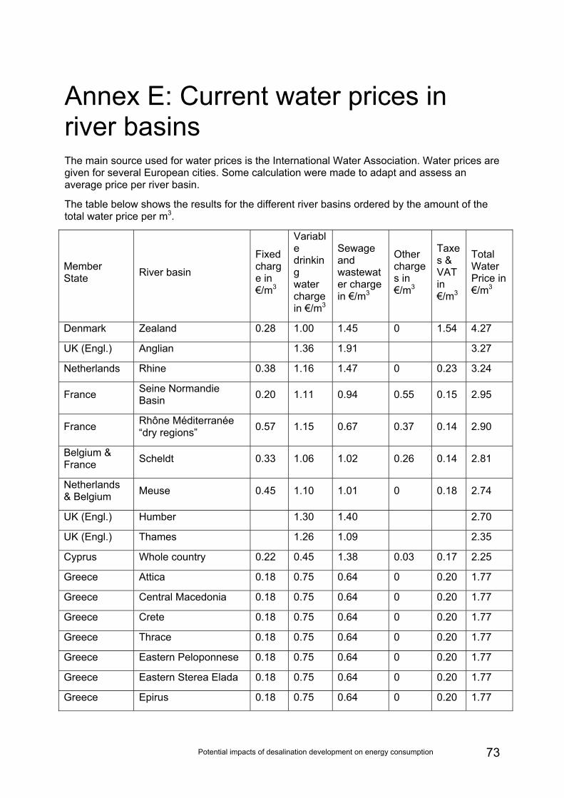
Potential impacts of desalination development on energy consumption 73
Annex E: Current water prices in river basins The main source used for water prices is the International Water Association. Water prices are given for several European cities. Some calculation were made to adapt and assess an average price per river basin.
The table below shows the results for the different river basins ordered by the amount of the total water price per m3.
Member State River basin
Fixed charge in €/m3
Variable drinking water charge in €/m3
Sewage and wastewater charge in €/m3
Other charges in €/m3
Taxes & VAT in €/m3
Total Water Price in €/m3
Denmark Zealand 0.28 1.00 1.45 0 1.54 4.27
UK (Engl.) Anglian 1.36 1.91 3.27
Netherlands Rhine 0.38 1.16 1.47 0 0.23 3.24
France Seine Normandie Basin 0.20 1.11 0.94 0.55 0.15 2.95
France Rhône Méditerranée “dry regions” 0.57 1.15 0.67 0.37 0.14 2.90
Belgium & France Scheldt 0.33 1.06 1.02 0.26 0.14 2.81
Netherlands & Belgium Meuse 0.45 1.10 1.01 0 0.18 2.74
UK (Engl.) Humber 1.30 1.40 2.70
UK (Engl.) Thames 1.26 1.09 2.35
Cyprus Whole country 0.22 0.45 1.38 0.03 0.17 2.25
Greece Attica 0.18 0.75 0.64 0 0.20 1.77
Greece Central Macedonia 0.18 0.75 0.64 0 0.20 1.77
Greece Crete 0.18 0.75 0.64 0 0.20 1.77
Greece Thrace 0.18 0.75 0.64 0 0.20 1.77
Greece Eastern Peloponnese 0.18 0.75 0.64 0 0.20 1.77
Greece Eastern Sterea Elada 0.18 0.75 0.64 0 0.20 1.77
Greece Epirus 0.18 0.75 0.64 0 0.20 1.77
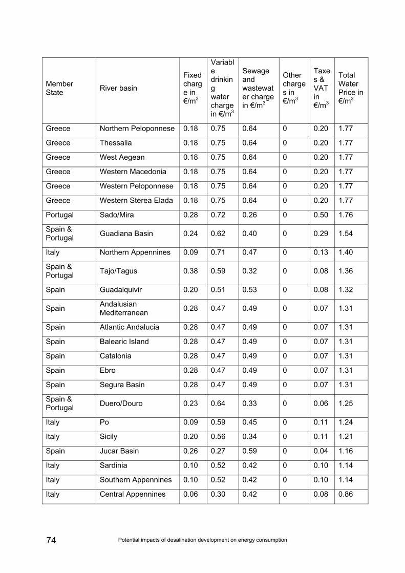
Potential impacts of desalination development on energy consumption 74
Member State River basin
Fixed charge in €/m3
Variable drinking water charge in €/m3
Sewage and wastewater charge in €/m3
Other charges in €/m3
Taxes & VAT in €/m3
Total Water Price in €/m3
Greece Northern Peloponnese 0.18 0.75 0.64 0 0.20 1.77
Greece Thessalia 0.18 0.75 0.64 0 0.20 1.77
Greece West Aegean 0.18 0.75 0.64 0 0.20 1.77
Greece Western Macedonia 0.18 0.75 0.64 0 0.20 1.77
Greece Western Peloponnese 0.18 0.75 0.64 0 0.20 1.77
Greece Western Sterea Elada 0.18 0.75 0.64 0 0.20 1.77
Portugal Sado/Mira 0.28 0.72 0.26 0 0.50 1.76
Spain & Portugal Guadiana Basin 0.24 0.62 0.40 0 0.29 1.54
Italy Northern Appennines 0.09 0.71 0.47 0 0.13 1.40
Spain & Portugal Tajo/Tagus 0.38 0.59 0.32 0 0.08 1.36
Spain Guadalquivir 0.20 0.51 0.53 0 0.08 1.32
Spain Andalusian Mediterranean 0.28 0.47 0.49 0 0.07 1.31
Spain Atlantic Andalucia 0.28 0.47 0.49 0 0.07 1.31
Spain Balearic Island 0.28 0.47 0.49 0 0.07 1.31
Spain Catalonia 0.28 0.47 0.49 0 0.07 1.31
Spain Ebro 0.28 0.47 0.49 0 0.07 1.31
Spain Segura Basin 0.28 0.47 0.49 0 0.07 1.31
Spain & Portugal Duero/Douro 0.23 0.64 0.33 0 0.06 1.25
Italy Po 0.09 0.59 0.45 0 0.11 1.24
Italy Sicily 0.20 0.56 0.34 0 0.11 1.21
Spain Jucar Basin 0.26 0.27 0.59 0 0.04 1.16
Italy Sardinia 0.10 0.52 0.42 0 0.10 1.14
Italy Southern Appennines 0.10 0.52 0.42 0 0.10 1.14
Italy Central Appennines 0.06 0.30 0.42 0 0.08 0.86
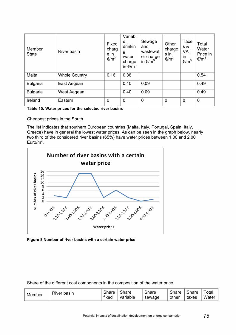
Potential impacts of desalination development on energy consumption 75
Member State River basin
Fixed charge in €/m3
Variable drinking water charge in €/m3
Sewage and wastewater charge in €/m3
Other charges in €/m3
Taxes & VAT in €/m3
Total Water Price in €/m3
Malta Whole Country 0.16 0.38 0.54
Bulgaria East Aegean 0.40 0.09 0.49
Bulgaria West Aegean 0.40 0.09 0.49
Ireland Eastern 0 0 0 0 0 0
Table 15: Water prices for the selected river basins
Cheapest prices in the South
The list indicates that southern European countries (Malta, Italy, Portugal, Spain, Italy, Greece) have in general the lowest water prices. As can be seen in the graph below, nearly two third of the considered river basins (65%) have water prices between 1.00 and 2.00 Euro/m3.
Figure 8 Number of river basins with a certain water price
Share of the different cost components in the composition of the water price
Member River basin Share fixed
Share variable
Share sewage
Share other
Share taxes
Total Water
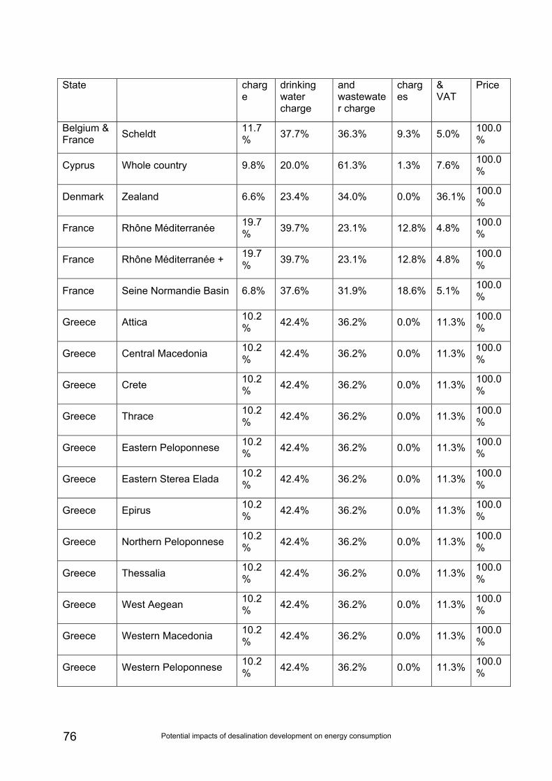
Potential impacts of desalination development on energy consumption 76
State charge
drinking water charge
and wastewater charge
charges
& VAT
Price
Belgium & France Scheldt 11.7
% 37.7% 36.3% 9.3% 5.0% 100.0%
Cyprus Whole country 9.8% 20.0% 61.3% 1.3% 7.6% 100.0%
Denmark Zealand 6.6% 23.4% 34.0% 0.0% 36.1% 100.0%
France Rhône Méditerranée 19.7% 39.7% 23.1% 12.8% 4.8% 100.0
%
France Rhône Méditerranée + 19.7% 39.7% 23.1% 12.8% 4.8% 100.0
%
France Seine Normandie Basin 6.8% 37.6% 31.9% 18.6% 5.1% 100.0%
Greece Attica 10.2% 42.4% 36.2% 0.0% 11.3% 100.0
%
Greece Central Macedonia 10.2% 42.4% 36.2% 0.0% 11.3% 100.0
%
Greece Crete 10.2% 42.4% 36.2% 0.0% 11.3% 100.0
%
Greece Thrace 10.2% 42.4% 36.2% 0.0% 11.3% 100.0
%
Greece Eastern Peloponnese 10.2% 42.4% 36.2% 0.0% 11.3% 100.0
%
Greece Eastern Sterea Elada 10.2% 42.4% 36.2% 0.0% 11.3% 100.0
%
Greece Epirus 10.2% 42.4% 36.2% 0.0% 11.3% 100.0
%
Greece Northern Peloponnese 10.2% 42.4% 36.2% 0.0% 11.3% 100.0
%
Greece Thessalia 10.2% 42.4% 36.2% 0.0% 11.3% 100.0
%
Greece West Aegean 10.2% 42.4% 36.2% 0.0% 11.3% 100.0
%
Greece Western Macedonia 10.2% 42.4% 36.2% 0.0% 11.3% 100.0
%
Greece Western Peloponnese 10.2% 42.4% 36.2% 0.0% 11.3% 100.0
%
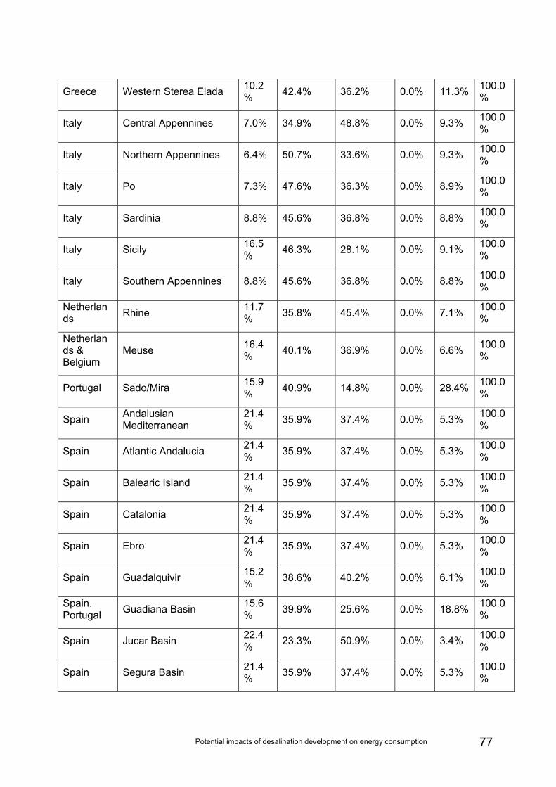
Potential impacts of desalination development on energy consumption 77
Greece Western Sterea Elada 10.2% 42.4% 36.2% 0.0% 11.3% 100.0
%
Italy Central Appennines 7.0% 34.9% 48.8% 0.0% 9.3% 100.0%
Italy Northern Appennines 6.4% 50.7% 33.6% 0.0% 9.3% 100.0%
Italy Po 7.3% 47.6% 36.3% 0.0% 8.9% 100.0%
Italy Sardinia 8.8% 45.6% 36.8% 0.0% 8.8% 100.0%
Italy Sicily 16.5% 46.3% 28.1% 0.0% 9.1% 100.0
%
Italy Southern Appennines 8.8% 45.6% 36.8% 0.0% 8.8% 100.0%
Netherlands Rhine 11.7
% 35.8% 45.4% 0.0% 7.1% 100.0%
Netherlands & Belgium
Meuse 16.4% 40.1% 36.9% 0.0% 6.6% 100.0
%
Portugal Sado/Mira 15.9% 40.9% 14.8% 0.0% 28.4% 100.0
%
Spain Andalusian Mediterranean
21.4% 35.9% 37.4% 0.0% 5.3% 100.0
%
Spain Atlantic Andalucia 21.4% 35.9% 37.4% 0.0% 5.3% 100.0
%
Spain Balearic Island 21.4% 35.9% 37.4% 0.0% 5.3% 100.0
%
Spain Catalonia 21.4% 35.9% 37.4% 0.0% 5.3% 100.0
%
Spain Ebro 21.4% 35.9% 37.4% 0.0% 5.3% 100.0
%
Spain Guadalquivir 15.2% 38.6% 40.2% 0.0% 6.1% 100.0
%
Spain. Portugal Guadiana Basin 15.6
% 39.9% 25.6% 0.0% 18.8% 100.0%
Spain Jucar Basin 22.4% 23.3% 50.9% 0.0% 3.4% 100.0
%
Spain Segura Basin 21.4% 35.9% 37.4% 0.0% 5.3% 100.0
%
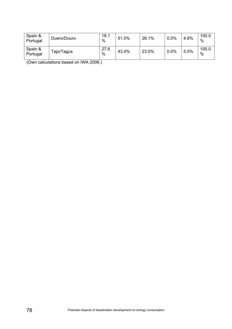
Potential impacts of desalination development on energy consumption 78
Spain & Portugal Duero/Douro 18.1
% 51.0% 26.1% 0.0% 4.8% 100.0%
Spain & Portugal Tajo/Tagus 27.6
% 43.4% 23.5% 0.0% 5.5% 100.0%
(Own calculations based on IWA 2006.)
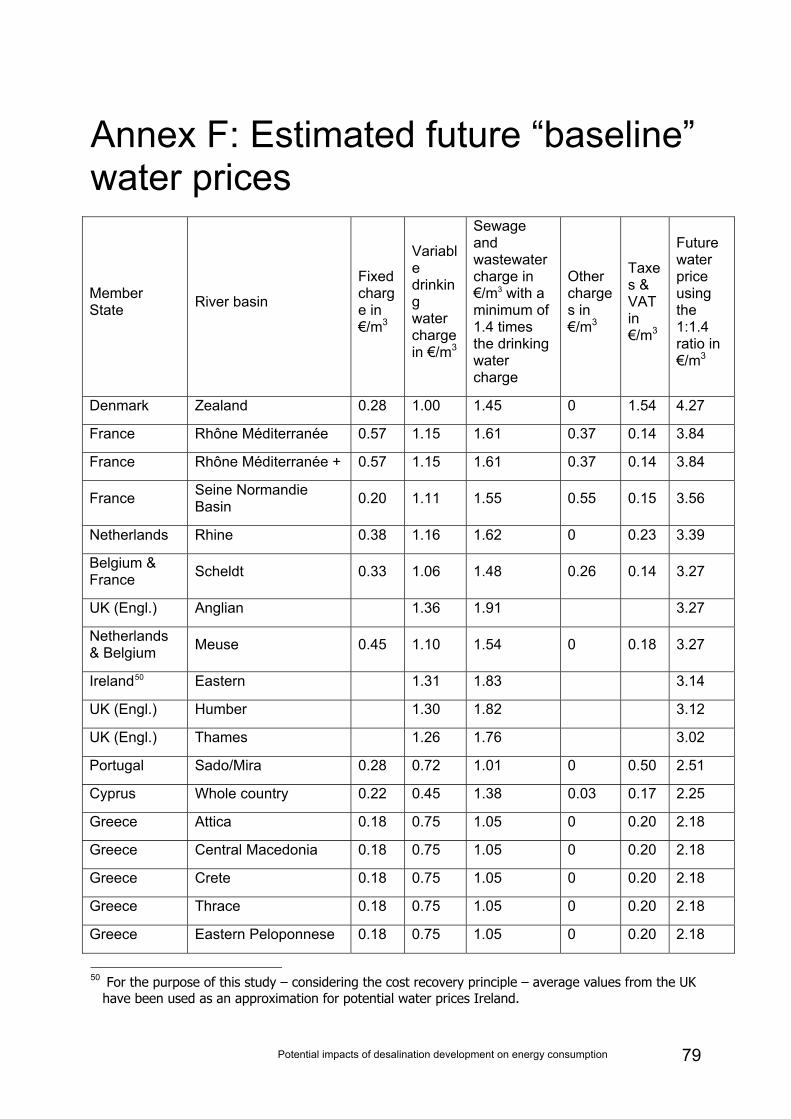
Potential impacts of desalination development on energy consumption 79
Annex F: Estimated future “baseline” water prices
Member State River basin
Fixed charge in €/m3
Variable drinking water charge in €/m3
Sewage and wastewater charge in €/m3 with a minimum of 1.4 times the drinking water charge
Other charges in €/m3
Taxes & VAT in €/m3
Future water price using the 1:1.4 ratio in €/m3
Denmark Zealand 0.28 1.00 1.45 0 1.54 4.27
France Rhône Méditerranée 0.57 1.15 1.61 0.37 0.14 3.84
France Rhône Méditerranée + 0.57 1.15 1.61 0.37 0.14 3.84
France Seine Normandie Basin 0.20 1.11 1.55 0.55 0.15 3.56
Netherlands Rhine 0.38 1.16 1.62 0 0.23 3.39
Belgium & France Scheldt 0.33 1.06 1.48 0.26 0.14 3.27
UK (Engl.) Anglian 1.36 1.91 3.27
Netherlands & Belgium Meuse 0.45 1.10 1.54 0 0.18 3.27
Ireland50 Eastern 1.31 1.83 3.14
UK (Engl.) Humber 1.30 1.82 3.12
UK (Engl.) Thames 1.26 1.76 3.02
Portugal Sado/Mira 0.28 0.72 1.01 0 0.50 2.51
Cyprus Whole country 0.22 0.45 1.38 0.03 0.17 2.25
Greece Attica 0.18 0.75 1.05 0 0.20 2.18
Greece Central Macedonia 0.18 0.75 1.05 0 0.20 2.18
Greece Crete 0.18 0.75 1.05 0 0.20 2.18
Greece Thrace 0.18 0.75 1.05 0 0.20 2.18
Greece Eastern Peloponnese 0.18 0.75 1.05 0 0.20 2.18
50 For the purpose of this study – considering the cost recovery principle – average values from the UK
have been used as an approximation for potential water prices Ireland.
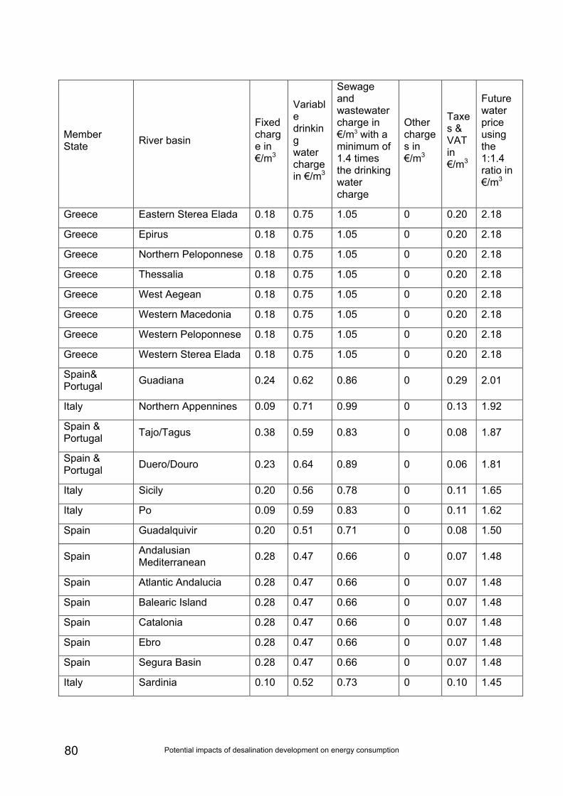
Potential impacts of desalination development on energy consumption 80
Member State River basin
Fixed charge in €/m3
Variable drinking water charge in €/m3
Sewage and wastewater charge in €/m3 with a minimum of 1.4 times the drinking water charge
Other charges in €/m3
Taxes & VAT in €/m3
Future water price using the 1:1.4 ratio in €/m3
Greece Eastern Sterea Elada 0.18 0.75 1.05 0 0.20 2.18
Greece Epirus 0.18 0.75 1.05 0 0.20 2.18
Greece Northern Peloponnese 0.18 0.75 1.05 0 0.20 2.18
Greece Thessalia 0.18 0.75 1.05 0 0.20 2.18
Greece West Aegean 0.18 0.75 1.05 0 0.20 2.18
Greece Western Macedonia 0.18 0.75 1.05 0 0.20 2.18
Greece Western Peloponnese 0.18 0.75 1.05 0 0.20 2.18
Greece Western Sterea Elada 0.18 0.75 1.05 0 0.20 2.18
Spain& Portugal Guadiana 0.24 0.62 0.86 0 0.29 2.01
Italy Northern Appennines 0.09 0.71 0.99 0 0.13 1.92
Spain & Portugal Tajo/Tagus 0.38 0.59 0.83 0 0.08 1.87
Spain & Portugal Duero/Douro 0.23 0.64 0.89 0 0.06 1.81
Italy Sicily 0.20 0.56 0.78 0 0.11 1.65
Italy Po 0.09 0.59 0.83 0 0.11 1.62
Spain Guadalquivir 0.20 0.51 0.71 0 0.08 1.50
Spain Andalusian Mediterranean 0.28 0.47 0.66 0 0.07 1.48
Spain Atlantic Andalucia 0.28 0.47 0.66 0 0.07 1.48
Spain Balearic Island 0.28 0.47 0.66 0 0.07 1.48
Spain Catalonia 0.28 0.47 0.66 0 0.07 1.48
Spain Ebro 0.28 0.47 0.66 0 0.07 1.48
Spain Segura Basin 0.28 0.47 0.66 0 0.07 1.48
Italy Sardinia 0.10 0.52 0.73 0 0.10 1.45
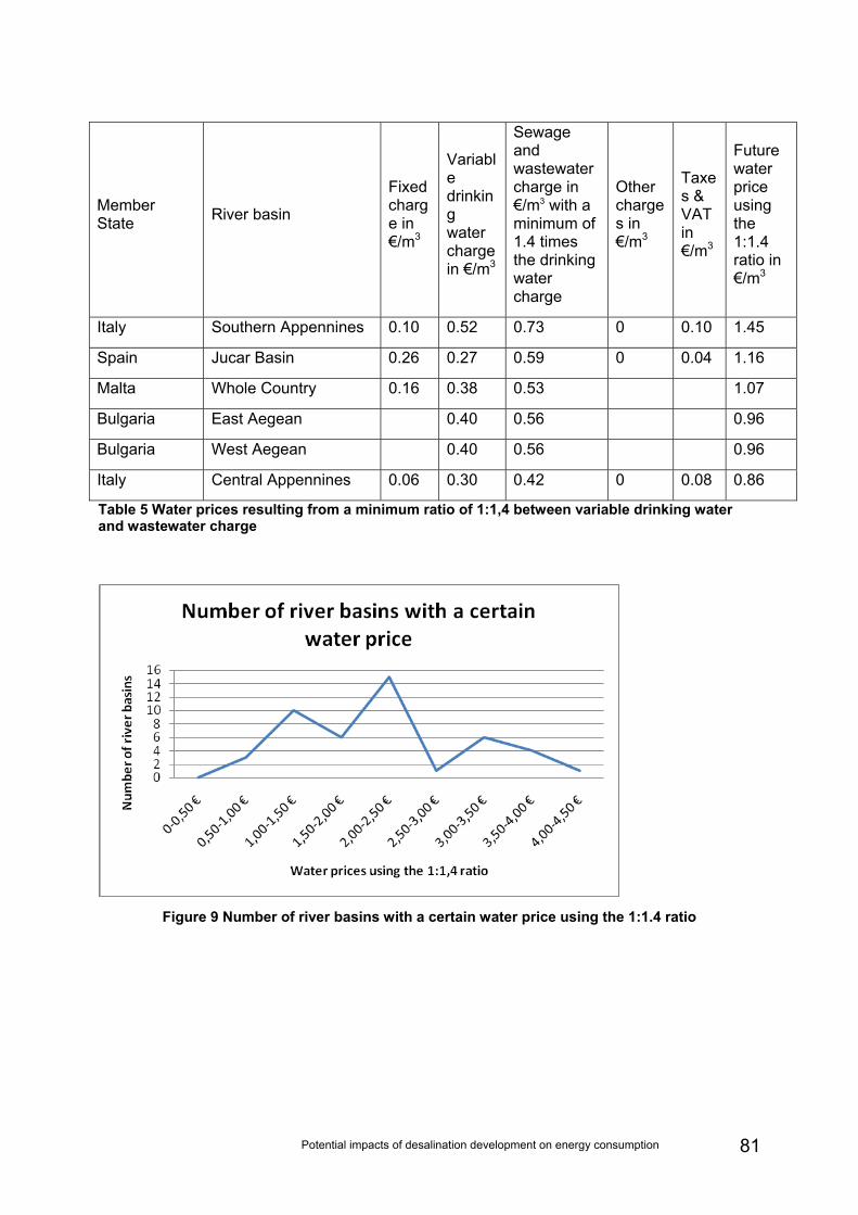
Potential impacts of desalination development on energy consumption 81
Member State River basin
Fixed charge in €/m3
Variable drinking water charge in €/m3
Sewage and wastewater charge in €/m3 with a minimum of 1.4 times the drinking water charge
Other charges in €/m3
Taxes & VAT in €/m3
Future water price using the 1:1.4 ratio in €/m3
Italy Southern Appennines 0.10 0.52 0.73 0 0.10 1.45
Spain Jucar Basin 0.26 0.27 0.59 0 0.04 1.16
Malta Whole Country 0.16 0.38 0.53 1.07
Bulgaria East Aegean 0.40 0.56 0.96
Bulgaria West Aegean 0.40 0.56 0.96
Italy Central Appennines 0.06 0.30 0.42 0 0.08 0.86
Table 5 Water prices resulting from a minimum ratio of 1:1,4 between variable drinking water and wastewater charge
Figure 9 Number of river basins with a certain water price using the 1:1.4 ratio
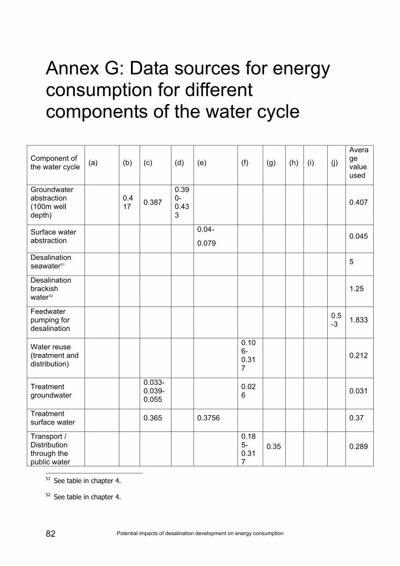
Potential impacts of desalination development on energy consumption 82
Annex G: Data sources for energy consumption for different components of the water cycle
Component of the water cycle (a) (b) (c) (d) (e) (f) (g) (h) (i) (j)
Average value used
Groundwater abstraction (100m well depth)
0.417 0.387
0.390-0.433
0.407
Surface water abstraction
0.04-
0.079 0.045
Desalination seawater51 5
Desalination brackish water52
1.25
Feedwater pumping for desalination
0.5-3 1.833
Water reuse (treatment and distribution)
0.106-0.317
0.212
Treatment groundwater
0.033-0.039-0.055
0.026 0.031
Treatment surface water 0.365 0.3756 0.37
Transport / Distribution through the public water
0.185-0.317
0.35 0.289
51 See table in chapter 4.
52 See table in chapter 4.
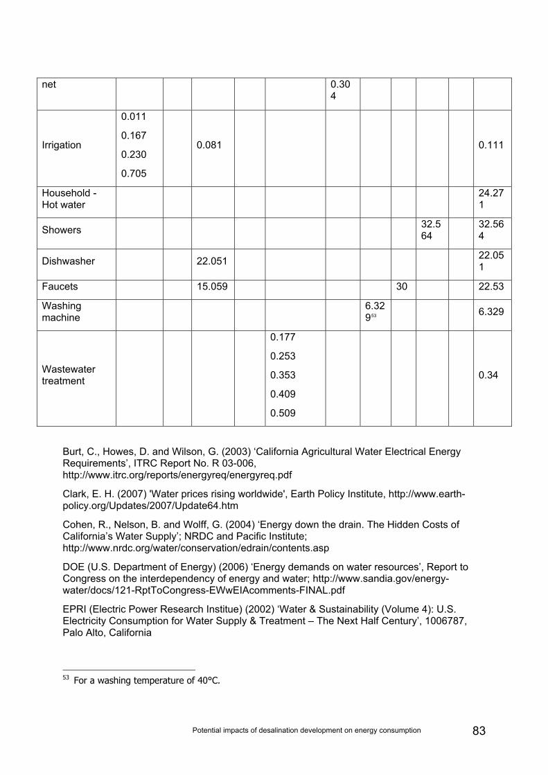
Potential impacts of desalination development on energy consumption 83
net 0.304
Irrigation
0.011
0.167
0.230
0.705
0.081 0.111
Household - Hot water
24.271
Showers 32.564
32.564
Dishwasher 22.051 22.051
Faucets 15.059 30 22.53
Washing machine
6.32953 6.329
Wastewater treatment
0.177
0.253
0.353
0.409
0.509
0.34
Burt, C., Howes, D. and Wilson, G. (2003) ‘California Agricultural Water Electrical Energy Requirements’, ITRC Report No. R 03-006, http://www.itrc.org/reports/energyreq/energyreq.pdf
Clark, E. H. (2007) 'Water prices rising worldwide', Earth Policy Institute, http://www.earth-policy.org/Updates/2007/Update64.htm
Cohen, R., Nelson, B. and Wolff, G. (2004) ‘Energy down the drain. The Hidden Costs of California’s Water Supply’; NRDC and Pacific Institute; http://www.nrdc.org/water/conservation/edrain/contents.asp
DOE (U.S. Department of Energy) (2006) ‘Energy demands on water resources’, Report to Congress on the interdependency of energy and water; http://www.sandia.gov/energy-water/docs/121-RptToCongress-EWwEIAcomments-FINAL.pdf
EPRI (Electric Power Research Institue) (2002) ‘Water & Sustainability (Volume 4): U.S. Electricity Consumption for Water Supply & Treatment – The Next Half Century’, 1006787, Palo Alto, California
53 For a washing temperature of 40°C.
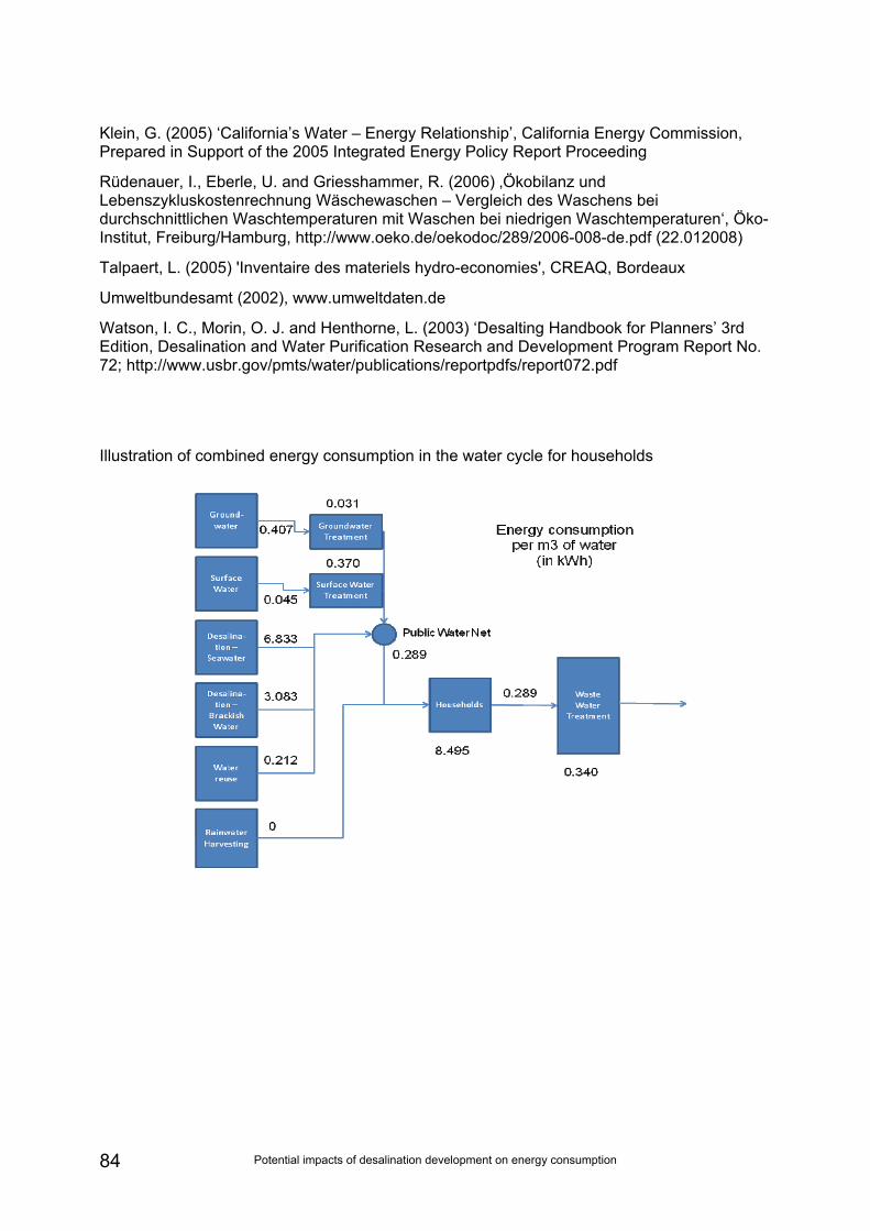
Potential impacts of desalination development on energy consumption 84
Klein, G. (2005) ‘California’s Water – Energy Relationship’, California Energy Commission, Prepared in Support of the 2005 Integrated Energy Policy Report Proceeding
Rüdenauer, I., Eberle, U. and Griesshammer, R. (2006) ‚Ökobilanz und Lebenszykluskostenrechnung Wäschewaschen – Vergleich des Waschens bei durchschnittlichen Waschtemperaturen mit Waschen bei niedrigen Waschtemperaturen‘, Öko-Institut, Freiburg/Hamburg, http://www.oeko.de/oekodoc/289/2006-008-de.pdf (22.012008)
Talpaert, L. (2005) 'Inventaire des materiels hydro-economies', CREAQ, Bordeaux
Umweltbundesamt (2002), www.umweltdaten.de
Watson, I. C., Morin, O. J. and Henthorne, L. (2003) ‘Desalting Handbook for Planners’ 3rd Edition, Desalination and Water Purification Research and Development Program Report No. 72; http://www.usbr.gov/pmts/water/publications/reportpdfs/report072.pdf
Illustration of combined energy consumption in the water cycle for households
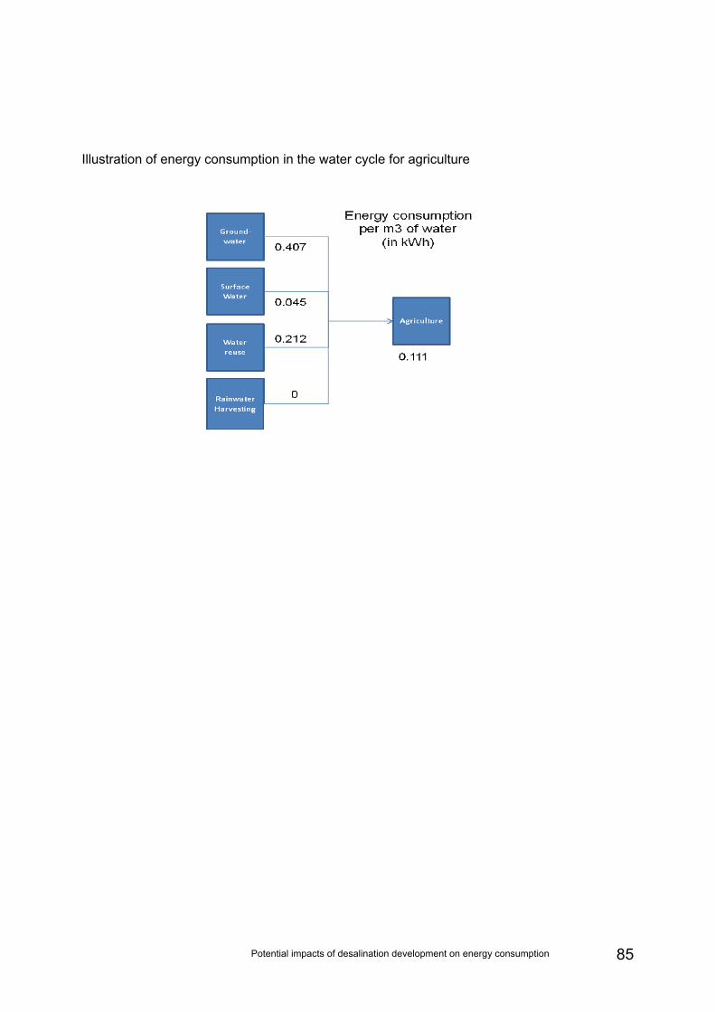
Potential impacts of desalination development on energy consumption 85
Illustration of energy consumption in the water cycle for agriculture
Potential impacts of desalination development on energy consumption 86
The Institute for European Environmental Policy (IEEP) 28 Queen Anne’s Gate SW1H 9AB London, UK Tel: +44 (0)20 7799 2244 Quai au Foin 55 1000 Brussels, Belgium Tel: +32 (0)23 738 7482
Email: [email protected] www.ieep.eu © IEEP 2008 All rights reserved.