USPS-RM2015-7/1

Report on the City Carrier Street Time Study

December 2014

Postal Regulatory CommissionSubmitted 12/11/2014 2:09:24 PMFiling ID: 90869Accepted 12/11/2014

USPS-RM2015-7/1

i

Table of Contents

I. INTRODUCTION ............................................................................................ 1

II. CONSTRUCTING THE COST POOLS ........................................................... 3

A. Introduction ................................................................................................ 3 B. The Route Evaluation Data System ........................................................... 4 C. Linking the Route Evaluation Data to the Street Time Cost Model ............. 6 D. Description of the Form 3999 Data Set ...................................................... 9 E. Calculating the Time Proportions for Cost Pool Formation ...................... 14

III. ESTIMATING THE REGULAR DELIVERY EQUATION AND CALCULATING THE ASSOCIATED VARIABILITIES ................................... 19

A. Introduction ............................................................................................. 19 B. Specifying the Regular Delivery Equation to Be Estimated ..................... 21 C. The Collection Volume Study .................................................................. 27 D. Creation of the Analysis Data Set ........................................................... 41 E. Estimation of the Model and Discussion of the Results .......................... 53

IV. ESTIMATING THE PACKAGE AND ACCOUNTABLE DELIVERY EQUATIONS AND CALCULATING THE ASSOCIATED

VARIABILITIES ............................................................................................. 85

A. Introduction ............................................................................................. 85 B. Specifying the Package and Accountable Models to be Estimated ........ 87 C. The Package and Accountable Field Study ............................................ 91 D. Constructing the Analysis Data Set .................................................... 101 E. Estimating the Econometric Models and Discussion of Results ............ 104

V. ASSESSING THE IMPACT OF THE STUDY ............................................ 118

USPS-RM2015-7/1

1

I. INTRODUCTION

The city carrier network is the largest part of the Postal Service’s delivery

network, incurring a total direct labor cost in Fiscal Year 2013 of almost $16 billion, of

which over $12 billion were in street time costs. These city carrier street time costs

represented 16.7 percent of total Postal Service costs.

The current development of attributable city carrier street time costs uses a

model that was calibrated with data collected in 2002. Since that time there have been

a number of important changes to city carrier delivery. These changes include the

widespread adoption of the delivery point sequencing (DPS) of letters, dramatic

changes in the volumes of mail delivered, restructuring of the city carrier network, and

the introduction of the flats sequencing system (FSS). Because of the importance of

city carrier street costs and the number of operational changes that have occurred, the

Postal Service initiated a comprehensive study of city carrier street time activities and

costs. This study has been used to update the existing city carrier street time model and

refine the calculation of the resulting attributable costs.

The production of city carrier street time attributable costs has three main steps,

which are illustrated in Figure 1. In the first step, the total accrued city carrier street

time costs are assigned to cost pools. This step breaks down total costs into the costs

associated with the different activities performed on the street, like delivering letter and

flats, or driving to and from the route. The relative sizes of the costs pools depend upon

the relative amount of time city carriers spend in the various activities.

USPS-RM2015-7/1

2

After the first step, the accrued costs are organized by cost pool, or activity. In

the next step, the total attributable costs for the various activities are calculated.

Attributable costs reflect the causal relationship between variations in mail volume and

responses in activity costs. These relationships are measured by estimating the relevant

variability or variabilities for each cost pool and then applying them to the cost pool’s

accrued cost. The last step is distributing the total attributable costs, by cost pool, to the

Accrued City Carrier Street Time Cost

Street Time Proportions

Accrued Costs by Cost Pool

Cost Pool Variabilities

Attributable Costs by Cost Pool

Distribution Keys

Attributable Costs by Product

Step1: Assign accrued street time costs to cost pools.

Step 2: Calculate attributable costs by cost pool.

Step 3: Distribute attributable costs to products.

Figure 1: Calculating Attributable Street Time Costs Has Three Steps

USPS-RM2015-7/1

3

individual products that cause them to arise. This step replies upon distribution keys

which measure the proportions of delivered volume for each product within each cost

pool.

This study updates and refines the first two steps in the process: determining the

cost pools and measuring the variabilities needed to calculate attributable costs. The

distribution keys needed to attribute costs to individual product are updated each year

with the Carrier Cost System and are not part of this study.

The next section of this report describes the use of operational data to measure

the street time proportions required for constructing the cost pools. That is followed by

a section then discusses estimating the variabilities for regular delivery. The subsequent

section that discusses estimating the variabilities for package and accountable delivery.

The last section presents the impact of the study on attributable costs.

II. CONSTRUCTING THE COST POOLS A. Introduction As explained above, an important component of the city carrier street time

costing process is the formation of cost pools. Cost pools reflect the activities that city

carriers perform on the street, such as driving to the route or delivering packages, and

capture the costs that are created by the performance of these activities.

The formation of cost pools requires identifying the proportions of city carrier

street time that are spent in the various activities. In fact, cost pools are formed by

multiplying those street proportions by the relevant accrued street time cost. In the

past, the time proportions were derived from expensive special studies that required

USPS-RM2015-7/1

4

collection of field data on all carrier activities. The Postal Service proposes replacing

those studies with data taken from its city carrier route evaluation system. This

approach has several advantages.

First, the route evaluation system covers virtually all city carrier routes in the

country, so the data set will be comprehensive. Second, because the data are based

upon actual operational practice, the resulting time proportions reflect the operational

reality of street time activity. Third, because the data can be extracted from an ongoing

data system, its production does not require an expensive special study, and the street

time proportions can be updated on a timely basis. Fourth, because they can be

updated regularly, time proportions based upon the route evaluation data automatically

reflect network and operational changes.

The balance of this section of the report describes the calculation of the time

proportions required for constructing the cost pools. First it presents a description of the

route evaluation system from which the data were drawn for updating the cost pools.

That discussion is followed by an explanation of how the route evaluation data relate to

the street time model. Next is a discussion of the actual data set used in the

calculations and the section ends with presentation of the new street time proportions.

B. The Route Evaluation Data System

The route evaluation data system consists of one observation for each city carrier

route in the country. The data come from when the route is evaluated. A route

evaluation is a process in which the Postal Service collects data on the times the carrier

spends in the various office and street activities on a route. Although the data are

USPS-RM2015-7/1

5

currently collected on an electronic data collection device, the structure of the street

time data obtained follows the format of Postal Service Form 3999.1 Thus, the street

time portion of route evaluation data is often called "Form 3999 data."

In order to form cost pools, a Form 3999 database was extracted from the Postal

Service's operational data systems in the spring of 2013, to match the period of time

when other data were drawn for estimating the regular delivery variabilities, as

discussed below. The Form 3999 data set used for this study includes route

evaluations for 140,457 city carrier routes. For each route, the most recent evaluation

in was used. These evaluations occurred primarily over the period from 2010 through

mid- 2013, as 99.5 percent of the evaluations in the database occurred over that three-

and- a-half year span. In addition, 96 percent of the evaluations occurred in the final

two-and-a-half years, from 2011 through mid- 2013. The evaluations therefore reflect

the relevant operating environment which incorporates the introduction of FSS, the

widespread deployment of DPS, and the Postal Service's efforts to rationalize its city

carrier network in the face of changes to mail volume and mail mix.

The route evaluation process includes recording the times that the carrier is

engaged in the various office and street activities, and a mail count conducted by the

delivery unit manager or designee. This process includes unannounced selective

checks on all of the routes being inspected to verify the accuracy of the mail count. In

addition, a route examiner makes a physical inspection of the route and then

accompanies the carrier for the full tour on the day of the inspection.

1 Prior to the use of the data collection devices, the street time portion of route evaluation data were collected manually on Form 3999.

USPS-RM2015-7/1

6

C. Linking the Route Evaluation Data to the Street Time Cost Model

The operations "view" of street activities is similar to, but not identical to the

street time cost model "view" of street activities. This means that a concordance

between the two views must be made to ensure accurate incorporation of the route

evaluation data into the cost model.

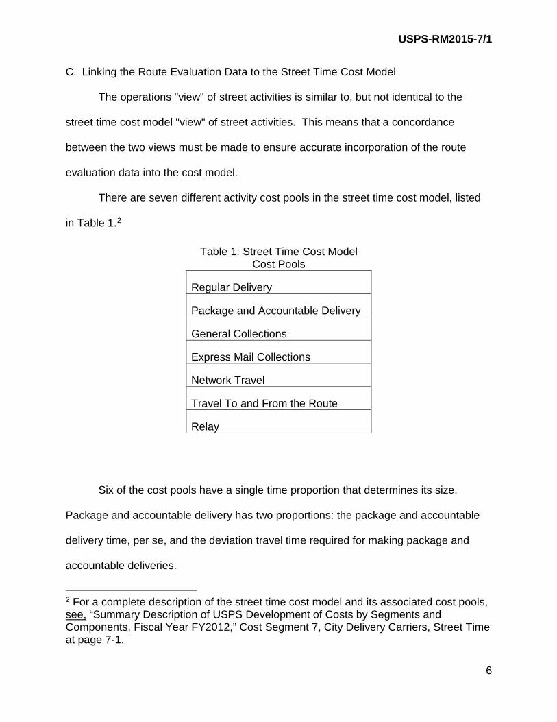
There are seven different activity cost pools in the street time cost model, listed

in Table 1.2

Table 1: Street Time Cost Model Cost Pools

Regular Delivery

Package and Accountable Delivery

General Collections

Express Mail Collections

Network Travel

Travel To and From the Route

Relay

Six of the cost pools have a single time proportion that determines its size.

Package and accountable delivery has two proportions: the package and accountable

delivery time, per se, and the deviation travel time required for making package and

accountable deliveries.

2 For a complete description of the street time cost model and its associated cost pools, see, “Summary Description of USPS Development of Costs by Segments and Components, Fiscal Year FY2012,” Cost Segment 7, City Delivery Carriers, Street Time at page 7-1.

USPS-RM2015-7/1

7

The listing of the operationally-defined activities that underlie the route evaluation

process is more detailed, but rolls up into the cost pool structure listed in Table 1.

There are sixteen different activities for which time is recorded in the route evaluation

process. These activities can be usefully classified in three ways. First, some of the

activities are directly attributable. This means they have individual time proportions in

the city carrier street time model and have a variabilities applied to them to find the

resulting attributable cost.3

Second, some of the activities are indirectly attributable. This means that they do

not have separate cost pools and/or variabilities. Instead, they take on the average

variability associated with the set of directly attributable activities. Finally, vehicle

loading and unloading are currently considered to be office time in the city carrier cost

model, and thus are not part of street time proportions. Figure 2 presents the route

evaluation activities and their classifications in the city carrier street time cost model.

3 These activities correspond to the cost pools listed in Table 1.

USPS-RM2015-7/1

8

Figure 2: Route Evaluation Activities and Their Cost Model Classifications

The directly attributable route evaluation activities match closely to the time

proportions used to form the city carrier cost model cost pools. In most cases, there is a

one-to-one correspondence between the route evaluation category and the street time

cost model time proportion. The concordance between the two is provided in Figure 3,

below:

Sector Segment

Relay Travel to Route Travel From Route Directly

Travel Within Attributable Accountable Delivery

Parcel Delivery Collection from SLB

Break

Deadhead Personal Needs Indirectly

Customer Contact Attributable Gas Vehicle

Non Recurring

Vehicle Load Office Vehicle Unload Time

USPS-RM2015-7/1

9

Figure 3: Linking Route Evaluation Activities and Cost Pools

Route Evaluation Activity Cost Model Time Proportion

D. Description of the Form 3999 Data Set The Form 3999 data set used to calculate the cost pools includes route

evaluations for 140,457 city carrier routes. The history of when those evaluations were

performed is presented in Table 2. Note that there are only 82 routes for which data

were captured prior to 2009. Because these routes represent only about one-twentieth

Sector Segment

Relay

Travel To

Travel From

Travel Within

Acct. Delivery

Parcel Delivery

Collection

Regular Delivery

Relay

Travel To/From Route

Network Travel

Parcel/Accountable Delivery

Collections from Street Letter Boxes

USPS-RM2015-7/1

10

of one percent of the data, they will be dropped from the subsequent analysis. That

leaves a working data set with 140,375 routes.

Table 2: History of Route Evaluations in the Form 3999 Data Base

Route Evaluations Proportions

2008 & Before 82 0.06%

2009 864 0.6%

2010 5,344 3.8%

2011 20,772 14.8%

2012 62,658 44.6%

2013 50,737 36.1% Total 140,457 100.0%

The next step is to examine the data to account for a set of small issues. For

example, 116 of the route evaluations reported data that were captured on Sunday. This

should not have occurred, and these evaluations are dropped. Also, 313 route

evaluations report a negative value for at least one of the directly attributable street time

activities. Obviously, this cannot occur, and must be due to a data entry error. These

evaluations are also dropped. Finally, 37 route evaluations report gross street time of

over 12 hours, and another 42 route evaluations report negative gross street time.

Because neither of these outcomes is possible, these route evaluations are also

dropped. In sum, eliminating these route evaluations because of data entry errors

reduces the data set by just 508 observations, leaving a total of 139,867 useful route

evaluations. The resulting analysis data set ends up using 99.6 percent of the raw data.

Gross street hours are defined as total street hours minus lunch. The average

value for gross street hours from the analysis data set is 6.14 hours. The relationship

USPS-RM2015-7/1

11

between the route evaluation data and the required time proportions for forming cost

pools is illustrated through the use of the concordance described in Figure 1, above.

That concordance is used to divide gross street hours into the city carrier cost model

proportions.

Table 3: Form 3999 Average Daily Hours Broken Out by Carrier Cost Model Definitions

Hours Proportion

Directly Attributable Street Hours 5.37 87.4%

Indirectly Attributable Street Hours 0.46 7.5%

Vehicle Load/Unload 0.31 5.1%

Gross Street Hours 6.14 100.0%

Cost pools need to be formed for the directly attributable street hours. This

requires taking the 5.37 hours from Table 3 and breaking them out into their component

parts. This, in turn, requires making use of the concordance presented in Figure 2 to

translate the route evaluation activities into the needed cost model activities, and then

calculating the proportion of time for each activity. This is done twice. First, it is done

for all of the route evaluations in the analysis dataset. Next, it is done for just the most

recent route evaluations, from 2012 and the first half of 2013, to determine if the

proportions of time spent in each activity are different when based upon only the most

recent evaluations. The results of those calculations are presented in Table 4, which

USPS-RM2015-7/1

12

shows the proportions for all route evaluations and the proportions for the 2012-2013

evaluations are very close to one another.

Table 4: Street Time Proportions Based upon Form 3999 Data

2012-2013 Route

Evaluations All Route

Evaluations

Regular Delivery 83.38% 83.20% Package/Accountable Delivery 4.63% 4.59%

Collections From SLB 0.20% 0.19%

Travel To/From Route 5.03% 5.03%

Network Travel 2.93% 3.01%

Relay 3.82% 3.94%

Number of Observations 112,972 139,867

When considering the use of Form 3999 data to calculate the street time

proportions, two questions arise. First, a route evaluation may come about because the

Postal Service is considering reconfiguring the routes in the ZIP Code. This means that

the data extracted from the route evaluation system could have been recorded before

the route was adjusted. If so, there is a concern that the Form 3999 data may not be

accurately representing the current route system. To assess the importance of this

concern, one can investigate how many route evaluations came before route

adjustment and how many came after route adjustment. Table 5 shows that a very high

USPS-RM2015-7/1

13

percentage came after the route was adjusted, with 76.7 percent of all route evaluations

coming after the latest route adjustment and 82.9 percent of route evaluations in the

2012-2013 period coming after the latest route adjustment. These high percentages

mitigate the concern that the Form 3999 data do not reflect the current network.

Table 5: Measuring the Proportion of Route Evaluations Coming After Route Adjustment

All Route Evaluations

2012-2013 Route

Evaluations

Routes With Data Captured After Adjustment 107,335 93,610

Total Routes 139,867 112,972

Proportion of Routes With Data Captured After Adjustment 76.7% 82.9%

The second question is how much the street time proportions change on a year-

by-year basis. The answer to this question addresses the issue of the utility of older

observations. In addition, looking at proportions of activities through time can help

gauge whether using some pre-adjustment route evaluation data is an issue of concern.

If route reconfigurations lead to material instability in the overall street time proportions,

then using pre-adjustment route evolution data could be a problem. On the other hand,

if the proportions are stable across years, then the reconfiguration of routes has not

affected the overall proportions of time and using pre-adjustment route evaluation data

is not a problem.

USPS-RM2015-7/1

14

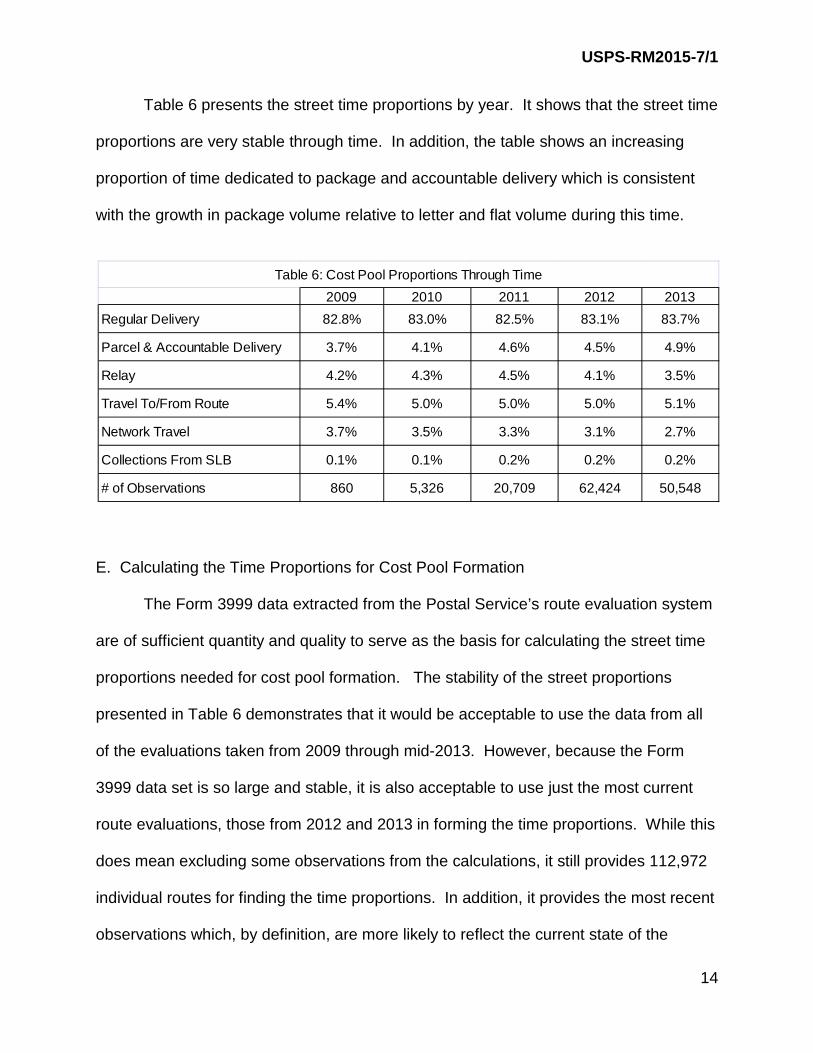
Table 6 presents the street time proportions by year. It shows that the street time

proportions are very stable through time. In addition, the table shows an increasing

proportion of time dedicated to package and accountable delivery which is consistent

with the growth in package volume relative to letter and flat volume during this time.

E. Calculating the Time Proportions for Cost Pool Formation The Form 3999 data extracted from the Postal Service’s route evaluation system

are of sufficient quantity and quality to serve as the basis for calculating the street time

proportions needed for cost pool formation. The stability of the street proportions

presented in Table 6 demonstrates that it would be acceptable to use the data from all

of the evaluations taken from 2009 through mid-2013. However, because the Form

3999 data set is so large and stable, it is also acceptable to use just the most current

route evaluations, those from 2012 and 2013 in forming the time proportions. While this

does mean excluding some observations from the calculations, it still provides 112,972

individual routes for finding the time proportions. In addition, it provides the most recent

observations which, by definition, are more likely to reflect the current state of the

2009 2010 2011 2012 2013Regular Delivery 82.8% 83.0% 82.5% 83.1% 83.7%

Parcel & Accountable Delivery 3.7% 4.1% 4.6% 4.5% 4.9%

Relay 4.2% 4.3% 4.5% 4.1% 3.5%

Travel To/From Route 5.4% 5.0% 5.0% 5.0% 5.1%

Network Travel 3.7% 3.5% 3.3% 3.1% 2.7%

Collections From SLB 0.1% 0.1% 0.2% 0.2% 0.2%

# of Observations 860 5,326 20,709 62,424 50,548

Table 6: Cost Pool Proportions Through Time

USPS-RM2015-7/1

15

network. Thus, although both the 2009-2013 proportions and the 2012-2013

proportions are acceptable (and quite similar), the more recent set of proportions will be

used in constructing the cost pools.

One final adjustment had to be made before the final time proportions could be

calculated. The route evaluation process is designed to produce information that is used

to configure carriers’ routes. To that end, it separately measures the time associated

with those packages that cause the carrier to deviate from the normal process of

delivery, because such packages are particularly important in calculating the time

requirement for the route. In contrast, the time for packages that fit in the mail

receptacle is included in regular delivery time, as their delivery is considered to be part

of the regular delivery process.

While this approach is entirely appropriate for a route configuration analysis, it

does not meet the needs of an attributable costing analysis. An attributable costing

analysis requires capturing the time for both deviation packages and those packages

that fit in the receptacle. This need is emphasized by the fact that there are more in-

receptacle packages than there are deviation packages. Consequently, the time

proportions based upon the Form 3999 data must be adjusted to account for the fact

that some of the time that the route evaluation process records for regular delivery is

actually time associated with delivery of in-receptacle packages.

The adjustment will be made with data collected in the package and accountable

field study described in Section IV, below. As part of that study, city carriers recorded

the amount of time they spent delivering in-receptacle packages, deviation packages,

and accountables. This total delivery time was compared to the total street time (for the

USPS-RM2015-7/1

16

same carriers on the same days) to calculate the proportion of total street time

dedicated to package and accountable delivery.4

Note that the data from the package and accountable field study provided the

package and accountable times as a proportion of total street time. But, as explained

above, to calculate cost pools one needs the package and accountable delivery time

proportions of directly attributable street time, which is a subset of total street time. To

find the correct proportions, an adjustment must be applied to the original total street

time proportions. The adjustment takes the following form: Suppose that one can

directly calculate the proportion that x1 is of a group of x’s, ranging from x1 through xp:

𝜌𝜌1 = 𝑥𝑥1

∑ 𝑥𝑥𝑖𝑖𝑝𝑝𝑖𝑖=1

.

However, further suppose that what is needed is x1 as a proportion of a subset of the

x’s, namely x1 through xq, where by definition, q < p:

𝜁𝜁1 = 𝑥𝑥1

∑ 𝑥𝑥𝑖𝑖𝑞𝑞𝑖𝑖=1

.

4 Note that total package and accountable delivery time incudes time for delivering both in receptacle and deviation packages. Also, the deviation time proportion needed for cost pool formation is deviation package and accountable delivery. The combined cost pool is required because a deviation delivery that requires a vehicle movement can involve the simultaneous delivery of both a deviation package and an accountable. Although the Form 3999 deviation package and accountable proportion (4.1%) is close to the corresponding field study proportion (4.7%), the package and accountable field study time for both deviation packages and (deviation) accountables will be used to ensure consistency.

USPS-RM2015-7/1

17

To obtain the desired proportion one need only take the originally calculated proportion

and multiply it by the ratio of the sums:

𝜁𝜁1 = �∑ 𝑥𝑥𝑖𝑖𝑝𝑝𝑖𝑖=1

∑ 𝑥𝑥𝑖𝑖𝑞𝑞𝑖𝑖=1

� 𝜌𝜌1.

In our case, the ratio of the sums is just the ratio of total street hours (6.14) to

directly attributable street hours (5.37). With this adjustment factor, the package and

accountable field study proportions of total street time can be converted to the

corresponding proportions of directly attributable street time. The two sets of

proportions, for both in-receptacle and deviation delivery are presented in Table 7.

Because directly attributable street time is smaller than total street time, recorded

package and accountable delivery time will be a higher proportion of directly attributable

time than of street time.

Table 7: Time Proportions Derived from the Package and Accountable Field Study

Type of Delivery Percentage of

Street Time

Ratio of Total Street Time to

Attributable Street Time

Percentage of Directly

Attributable Street Time

In Receptacle 3.84% 1.14 4.40%

Deviation 4.71% 1.14 5.39%

Both 8.55% 1.14 9.79%

The package and accountable delivery time proportions can now be used to

modify the street time proportions used to construct the cost pools. Because the route

USPS-RM2015-7/1

18

evaluation process incorporates in-receptacle package delivery time into regular

delivery time, the regular delivery time proportion is overstated for attributable costing

purposes. Accuracy requires using the independently measured in-receptacle package

delivery time proportion to reduce the route evaluation delivery time proportion. This

calculation is done in Table 8.

Table 8: Adjusting Time Proportions To Capture Total Package Delivery

Type of Delivery Form 3999 Only Including PA Study

Proportions

Regular Delivery 83.38% 78.23%

Package and Accountable Delivery 4.63% 9.79%

Total 88.01% 88.01%

With this adjustment of the regular delivery time proportion in place, the last step

is to incorporate the new regular delivery and package and accountable delivery into the

full set of street time proportions. The set of proportions used to calculate the cost

pools is presented in Table 9.

USPS-RM2015-7/1

19

Table 9 Street Time Proportions Used to Calculate Cost Pools

Street Activity Time Proportion Regular Delivery 78.23%

In-Receptacle Package Delivery 4.40%

Deviation Delivery 5.39%

Collection from Street Letter Boxes 0.20%

Travel To and From 5.03%

Relay 3.82%

Network Travel 2.93%

Total 100.0%

III. ESTIMATING THE REGULAR DELIVERY EQUATION AND CALCULATING THE ASSOCIATED VARIABILITIES

A. Introduction

Regular delivery time makes up the bulk of a city carrier’s street time and is the

largest cost pool in the street time cost model. It includes primary delivery activities like

driving along the route within delivery sections, accessing stops (whether on foot or in a

vehicle), putting letters and flats into customers' mail receptacles, and retrieving

collection mail from those receptacles.

As discussed above, the use of operational data to define the street time cost

pools required adopting an operations set of characterizations of street activities. The

operations definition of regular delivery time is a bit more expansive than the definition

USPS-RM2015-7/1

20

historically used in the street time cost model.5 This fact, by itself, suggests that a new

set of regular delivery time variabilities should be estimated in order to better align with

the regular delivery time obtained from the Form 3999 data set. In addition, there have

been a number of operational changes in delivery since the last time regular delivery

variabilities were estimated. These include the widespread use of delivery point

sequencing (DPS) of letters, the decline in delivered volumes and subsequent route

reconfigurations, and the deployment of flat sequencing systems (FSS) in many ZIP

Codes. FSS equipment sorts automation flat mail into delivery point sequence.

Taken together, these changes necessitate estimating new regular delivery

variabilities that are consistent with operations definitions of street activities and reflect

the current cost-causing characteristics of city carrier regular delivery. Estimating these

variabilities requires specifying a model of regular delivery, constructing the relevant

analysis data set, econometrically estimating the specified model with the analysis data

set, and then reviewing and evaluating the results.

The next subsection discusses the issues associated with model specification

and variable selection. Normally that would be followed by a subsection on constructing

the analysis data set, but because a special field study was required for obtaining

volumes of mail collected, the next subsection will be devoted to describing that study.

After that description, the expected subsection on constructing the analysis data set is

presented. The last subsection describes the estimation of the model and discusses

the results of that estimation.

5 In operations parlance, regular delivery time is often “sector segment” time.

USPS-RM2015-7/1

21

B. Specifying the Regular Delivery Equation to Be Estimated

A logical way to start the specification of the regular delivery equation is by

identifying the cost drivers of regular delivery time. In other words, this step involves

identifying the variables that determine regular delivery time and should thus be

included as explanatory variables in a regular delivery econometric equation.

Regular delivery time is caused both by the volumes that are delivered and by the need

to cover the network of delivery points. Consequently, the cost drivers of regular

delivery time6 are the volumes, delivered and collected, and the number of delivery

points in the network.7 In addition, regular delivery time could be influenced by the

technology of delivery and certain characteristics of the delivery area. In sum, the

regular delivery equation should include the relevant volume cost drivers, the number of

delivery points to be covered, and variables capturing the characteristics of the delivery

technology and the delivery area.

The volume cost drivers should reflect the way the mail is handled on the street.

In city carrier delivery, mail is handled in separate bundles on walking routes and in

separate containers on driving routes. Mail is selected from these bundles or containers

for placement in the mail receptacle. In other words, these bundles or containers define

how mail is handled on the street and these handlings generate regular delivery time.

6 Regular delivery time includes the collection of mail from customers' receptacles. It does not include the collection of mail from street letter boxes. That time is included in another cost pool. In this section, the terms "collection volume" or "volume collected" always refers to mail volume collected from customers' receptacles and not from street letter boxes. 7 The delivery points in the network are sometimes described as “possible” deliveries because they represent the possible delivery points that carriers must be prepared to cover. On any given day, not all possible delivery points will receive mail.

USPS-RM2015-7/1

22

The appropriate volume cost drivers should reflect this bundle structure and

include all city carrier delivered letters and flats. There are volume bundles for DPS

mail, cased mail, sequenced mail, FSS mail, and mail collected from customers and

these five types of mail are the volume cost drivers. Note that cased mail includes both

letters and flats, which are cased together and pulled down into one bundle or

container. In addition, there are some pieces which may be classified as packages by

the DMM, but are handled as flats by city carriers. These pieces are included in cased

mail.8

The other main driver of regular delivery cost is the need to cover the delivery

network. Some regular delivery costs arise because carriers traverse certain parts of

their routes on a daily basis. This time does not vary with small variations in volume but

does vary with the size of the network to be covered. This network structure implies

that the primary cost-causing characteristic of the network is the number of delivery

points to which the mail is delivered, and thus another cost driver included in the regular

delivery equation is the number of delivery points to be covered.

The Postal Service manages its city carrier network by ZIP Code. The total

hours required for a ZIP Code’s delivery function are caused by the ZIP Code’s volumes

and the number of delivery points included in the ZIP Code. While carrier routes are an

important organizing structure for the Postal Service, management decisions are made

at the ZIP Code level. This is highlighted by the widespread use of pivoting routes.

Pivoting takes place when a route’s delivery responsibilities are not handled by its

assigned carrier, but rather by other carriers in the ZIP Code. Throughout a week,

8 Recall that the time required for the delivery of packages (both in receptacle and deviation) is included in a separate cost pool.

USPS-RM2015-7/1

23

different routes may be pivoted on different days, reflecting the fluidity of the route

structure. Thus, to accurately capture the relationship between delivery time and

volume, the model should be estimated on ZIP Code level data.

The last set of variables included in the model are designed to capture variations

in the delivery environment that could cause differences in the amount of delivery time

required to deliver a given amount of volume to a set number of delivery points. These

variables are included in the equation to improve its ability to explain regular delivery

time and to ensure that the estimated coefficients on the volume variables do not

include any non-volume effects.

There are three main characteristics that describe the delivery environment: (1)

the primary delivery technology used in the ZIP Code, (2) the proportion of business

deliveries in the ZIP Code and the (3) geographical density of delivery points in the ZIP

Code. Each of these variables are introduced and explained below.

First, delivery technology is measured for a ZIP Code by examining the delivery

technology of the routes within that ZIP Code. Routes are classified as being one of

five types: curbline, dismount, foot, park and loop or other. 9

When identifying delivery technologies for costing purposes, the important

distinction is the one between those routes which primarily involve walking (Foot, Park

and Loop, and Other) and those routes which primarily involve driving (Curbline and

Dismount). Because walking is generally slower than driving, for a given amount of mail,

9 The delivery mode ‘other’ are for the extremely small number of routes that do not fit into one of the other four categories. Route on which a carrier uses a Segway or uses public transportation are examples of routes that have a delivery mode of ‘other’.

USPS-RM2015-7/1

24

delivery points, and geographical area, ZIP Codes made up of walking routes typically

have a greater amount of delivery time.

As such, a technology indicator can be constructed to capture whether a ZIP

Code is primarily a walking ZIP Code or driving ZIP Code. To construct this indicator,

each route in a ZIP Code is assigned a value of zero if it is a curbline or dismount route

(driving route) and a value of one if it is a foot, park and loop, or other route (walking

route). The technology indicator is then calculated as the percentage of walking routes

in the ZIP Code and has a range from zero through one. If a ZIP Code has all driving

routes, the indicator variable takes a value of zero. In contrast, if a ZIP Code has all

walking routes, the indicator variable takes a value of one. As the value of the indicator

variable goes up, ceteris paribus, regular delivery time should increase.

The next characteristic variable is included in the regular delivery equation to

control for the possibility that the time for delivering a given amount of mail to business

delivery points is different from the time needed for delivering the same amount of mail

to residential delivery points. In other words, this variable is included to allow the

econometric model to account for the possibility that ZIP Codes with many business

delivery points would have less delivery time for the same amount of delivered volume

and delivery points than similar ZIP Codes with few business deliveries. The

characteristic variable to capture this effect is calculated as the percentage of business

delivery points in the ZIP Code.

The last characteristic variable included in the equation is a measure of the

geographic density of the delivery area. The larger the geographic area included in the

ZIP Code, for a given number of delivery points, the more time is required to cover

USPS-RM2015-7/1

25

those delivery points.10 A measure of delivery density can be constructed from the

land area, in square miles, of each ZIP Code in the data set.11

The next step in preparing for estimation is choosing a functional form. If there is

technological or other knowledge about the underlying cost-generating process, it can

be used to guide functional form selection. If not, there are advantages to selecting a

flexible functional form when attempting to measure the responsiveness of cost to

volume changes. Finally, one can review previous work to identify functional form

selections for similar modeling efforts.

In the area of city carrier delivery, previous work has shown the quadratic

functional form to be useful.12 It has been used by both the Postal Service and the

Postal Regulatory Commission (Commission) to specify a number of different models of

delivery time. The quadratic functional form also has the advantage of being a flexible

functional form in the sense that it places no restrictions on the first and second order

derivatives. Thus it is agnostic, a priori, about the absence or presence of scale or

network economies that cause the variabilities to be less than one hundred percent.

10 For a discussion of the impact of density on delivery costs, see, Bernard, Stephane, Cohen, Robert, Robinson, Matthew, Roy, Bernard, Toledano, Joelle, Waller, John and Xenakis, Spyros, “Delivery Cost Heterogeneity and Vulnerability to Entry,” in Postal and Delivery Services: Delivering on Competition, Michael Crew and Paul Kleindorfer (eds.), Kluwer, 2002 11 Square miles of land area for all ZIP Codes were extracted from the 2010 Census. 12 For example, see Bradley, Michael D, Colvin, Jeff and Mary K. Perkins, “Measuring Scale and Scope Economies with A Structural Model of Postal Delivery,” in Liberalization of the Postal and Delivery Sector, Advances in Regulatory Economics Series, Edward Elgar, 2007, or “Testimony of Michael D. Bradley on Behalf of the United States Postal Service,” USPS-T-14, Docket No. R2005-1

USPS-RM2015-7/1

26

The primary alternative flexible functional form is the translog. However, because of

repeated instances in which one or more of the volume measures has a zero value, a

traditional translog cannot be used, as the log of zero is not defined. The Box-Cox

transformation can permit the estimation of logarithmic function but, given the previous

work employing the quadratic function, it is unnecessary to introduce this nonlinear

method of estimation.

Application of the quadratic functional form to the explanatory variables

described above yields the following model to be estimated:

𝐷𝐷𝐷𝐷𝑖𝑖𝑖𝑖 = 𝛽𝛽0 + 𝛽𝛽1 𝐷𝐷𝐷𝐷𝐷𝐷𝑖𝑖𝑖𝑖 + 𝛽𝛽11𝐷𝐷𝐷𝐷𝐷𝐷𝑖𝑖𝑖𝑖2 + 𝛽𝛽2 𝐶𝐶𝐶𝐶𝑖𝑖𝑖𝑖 + 𝛽𝛽21𝐶𝐶𝐶𝐶𝑖𝑖𝑖𝑖2 + 𝛽𝛽3 𝐷𝐷𝑆𝑆𝑆𝑆𝑖𝑖𝑖𝑖 + 𝛽𝛽31𝐷𝐷𝑆𝑆𝑆𝑆𝑖𝑖𝑖𝑖

2 + 𝛽𝛽4 𝐹𝐹𝐷𝐷𝐷𝐷𝑖𝑖𝑖𝑖+ 𝛽𝛽41𝐹𝐹𝐷𝐷𝐷𝐷𝑖𝑖𝑖𝑖

2 + 𝛽𝛽5 𝐶𝐶𝐶𝐶𝑖𝑖𝑖𝑖 + 𝛽𝛽51𝐶𝐶𝐶𝐶𝑖𝑖𝑖𝑖2 + 𝛽𝛽6 𝐷𝐷𝐷𝐷𝑖𝑖𝑖𝑖 + 𝛽𝛽61𝐷𝐷𝐷𝐷𝑖𝑖𝑖𝑖2 + 𝛽𝛽12 𝐷𝐷𝐷𝐷𝐷𝐷𝑖𝑖𝑖𝑖 ∗ 𝐶𝐶𝐶𝐶𝑖𝑖𝑖𝑖+ 𝛽𝛽13 𝐷𝐷𝐷𝐷𝐷𝐷𝑖𝑖𝑖𝑖 ∗ 𝐷𝐷𝑆𝑆𝑆𝑆𝑖𝑖𝑖𝑖 + 𝛽𝛽14 𝐷𝐷𝐷𝐷𝐷𝐷𝑖𝑖𝑖𝑖 ∗ 𝐹𝐹𝐷𝐷𝐷𝐷𝑖𝑖𝑖𝑖 + 𝛽𝛽15 𝐷𝐷𝐷𝐷𝐷𝐷𝑖𝑖𝑖𝑖 ∗ 𝐶𝐶𝐶𝐶𝑖𝑖𝑖𝑖 + 𝛽𝛽16 𝐷𝐷𝐷𝐷𝐷𝐷𝑖𝑖𝑖𝑖 ∗ 𝐷𝐷𝐷𝐷𝑖𝑖𝑖𝑖+ 𝛽𝛽23 𝐶𝐶𝐶𝐶𝑖𝑖𝑖𝑖 ∗ 𝐷𝐷𝑆𝑆𝑆𝑆𝑖𝑖𝑖𝑖 + 𝛽𝛽24 𝐶𝐶𝐶𝐶𝑖𝑖𝑖𝑖 ∗ 𝐹𝐹𝐷𝐷𝐷𝐷𝑖𝑖𝑖𝑖 + 𝛽𝛽25 𝐶𝐶𝐶𝐶𝑖𝑖𝑖𝑖 ∗ 𝐶𝐶𝐶𝐶𝑖𝑖𝑖𝑖 + 𝛽𝛽26 𝐶𝐶𝐶𝐶𝑖𝑖𝑖𝑖 ∗ 𝐷𝐷𝐷𝐷𝑖𝑖𝑖𝑖+ 𝛽𝛽34 𝐷𝐷𝑆𝑆𝑆𝑆𝑖𝑖𝑖𝑖 ∗ 𝐹𝐹𝐷𝐷𝐷𝐷𝑖𝑖𝑖𝑖 + 𝛽𝛽35 𝐷𝐷𝑆𝑆𝑆𝑆𝑖𝑖𝑖𝑖 ∗ 𝐶𝐶𝐶𝐶𝑖𝑖𝑖𝑖 + 𝛽𝛽36 𝐷𝐷𝑆𝑆𝑆𝑆𝑖𝑖𝑖𝑖 ∗ 𝐷𝐷𝐷𝐷𝑖𝑖𝑖𝑖 + 𝛽𝛽45 𝐹𝐹𝐷𝐷𝐷𝐷𝑖𝑖𝑖𝑖 ∗ 𝐶𝐶𝐶𝐶𝑖𝑖𝑖𝑖+ 𝛽𝛽46 𝐹𝐹𝐷𝐷𝐷𝐷𝑖𝑖𝑖𝑖 ∗ 𝐷𝐷𝐷𝐷𝑖𝑖𝑖𝑖 + 𝛽𝛽5 𝐶𝐶𝐶𝐶𝑖𝑖𝑖𝑖 ∗ 𝐷𝐷𝐷𝐷𝑖𝑖𝑖𝑖 + 𝛽𝛽7 𝐷𝐷𝐶𝐶𝑖𝑖𝑖𝑖 + 𝛽𝛽71𝐷𝐷𝐶𝐶𝑖𝑖𝑖𝑖

2 + 𝛽𝛽8 𝐶𝐶𝐷𝐷𝐷𝐷𝐷𝐷𝑖𝑖𝑖𝑖+ 𝛽𝛽81𝐶𝐶𝐷𝐷𝐷𝐷𝐷𝐷𝑖𝑖𝑖𝑖2 + 𝛽𝛽9 𝐵𝐵𝐵𝐵𝑖𝑖𝑖𝑖 + 𝛽𝛽91𝐵𝐵𝐵𝐵𝑖𝑖𝑖𝑖2 + 𝜀𝜀𝑖𝑖𝑖𝑖

Where:

DT = Regular Delivery Time DPS = Delivery Point Sequenced Letters CM = Cased Mail SEQ = Sequenced Mail FSS = FSS Flats CV = Collection Volume DP = Delivery Points DM = Delivery Mode Indicator MPDP = Miles per Delivery Point BR = Proportion of Business Deliveries

USPS-RM2015-7/1

27

C. The Collection Volume Study Once an econometric equation is specified, the normal next step is to construct

the analysis data with which the equation’s coefficients will be estimated. However, the

Postal Service’s carrier data systems do not include counts of volumes collected from

customers by city carriers, so a special study was required to complete the analysis

data set. This subsection describes that special study.

Regular delivery time is simultaneously influenced by both the letter and flat mail

delivered to customers’ receptacles and the mail collected from those receptacles. The

analysis data set used to estimate the regular delivery equation should thus include

both delivered and collected volumes for a single set of addresses. The Postal Service

performed a field study to obtain collection volumes that were subsequently matched

with delivery volumes. The collection and delivery volumes were both from the same

ZIP Codes, routes and days, and combining them produced the complete set of volume

measures required for estimating the regular delivery equation.

The field study that obtained the collection volumes was carried out with the

following steps:

1. The sample was developed.

2. The study process was designed.

3. A beta test of the study was performed and the study process was refined.

4. The full data collection effort was launched.

5. The collected data were analyzed.

6. The collection volumes were combined with delivery volumes.

USPS-RM2015-7/1

28

Each of these steps is discussed in the following subsections.

1. Developing the sample A sample size of 300 ZIP Codes was determined to be the largest sample

consistent with Postal Service budgetary and management resources. This is

approximately double the sample sizes of previous city carrier studies and, when

combined with the delivery data, provided a substantially larger analysis dataset than

was available in past work on carrier costs. To increase the efficiency of the sampling,

the collection volume study utilized a stratified systematic sample from a frame of

10,720 ZIP Codes that contain city carrier routes.

Two variables, which are highly correlated with a ZIP Code’s street time, were

used to stratify the data into six subdivisions. Those two variables are number of routes

in the ZIP Code and its overall delivery mode, as either a "driving” ZIP Code or a

"walking” ZIP Code. A driving ZIP Code has mostly curbline or dismount routes and a

walking ZIP Code has mostly foot or park and loop routes. Details about the

development of the sample are included in USPS-RM2015-7/1 but the six subdivisions

and their stratum proportions a presented in Table 10.

USPS-RM2015-7/1

29

2. Designing the study process

The study’s goal was to obtain a set of ZIP Code collection mail volumes that

corresponded to those ZIP Code’s delivered volumes, as reported in Postal Service’s

Delivery Operations Information System (DOIS) over a two-week period. The field

study thus had city carriers record collection volumes, by source and shape, for twelve

Stratum Definition # of ZIPs

Stratum Proportion of

Time Driving ZIP

x < 6 routes

Walking ZIP

x < 6 routes

Driving ZIP

5 < x < 21 routes

Driving ZIP

5 < x < 21 routes

Driving ZIP

x > 20 routes

Walking ZIP

x > 20 routes

The Stratum Proportions Table 10

Large Driving 882 18%

Large Walking 1,501 32%

Medium Driving 2,254 20%

Medium Walking 2,787 24%

Small Driving 1,209 2%

Small Walking 2,087 4%

USPS-RM2015-7/1

30

consecutive delivery days.13 To ensure accurate data collection, operations experts

were integrated into the study process, in terms of both designing and implementing

the study. This greatly increased field participation.

Because of the large number of ZIP Codes included in the study, a decentralized

study team structure was employed. Headquarters coordinators worked with area

coordinators who facilitated the study by identifying and working with local

coordinators. The local coordinators supervised the carriers participating in the study

and were responsible for ensuring their ZIP Code's data were correctly recorded and

entered. Training was conducted prior to implementation to ensure consistent and

accurate data collection. Prior to beginning the study, headquarters coordinators

trained both the area and local coordinators. Local coordinators then trained individual

carriers. The training materials are included in USPS-RM2015-7/1.

There are three possible sources of collection mail for letter carriers: (1) mail

received directly from customer receptacles, (2) mail received in collection points (like

mail chutes), and (3) containerized mail received from businesses. To guarantee

complete coverage of collection volumes, the study required carriers to measure their

mail collected from all three sources. Discussions with operations experts lead to the

determination that the study would provide the most accurate results if collection mail

volume for letters and flats were recorded in linear measurements, using quarter inch

increments, and piece counts were to be used for packages. While letter and flat mail

can be collected from any of the three sources, packages are not collected in

13 Because regular delivery time is incurred only by city carriers with regular letter routes, the sample does not include volumes collected by special purpose route (SPR) carriers. The time required for collecting that mail is included in a separate cost pool that is not part of this study.

USPS-RM2015-7/1

31

containers from businesses. As a result, carriers were required to record volumes by

eight different combinations of shape and source.

3. Performing a beta test

To ensure that the study process produced accurate data, the Postal Service

performed a beta test at a small number of ZIP Codes in March, 2013. The beta test

was used to evaluate the study forms, instructions, and procedures. This evaluation

was done to allow, if necessary, refinement of the procedures for the full study In

addition, examination of the data from the beta test served as a “proof of concept” of the

study process before launching the full study.

The beta test took place at five ZIP Codes, including 116 city carrier routes.

Collection volumes were measured for six days on each route. This means there was a

potential data set of 696 route days of volume. The Postal Service was able to collect

data for 695 of the 696 route days, missing only one route day.

The beta test revealed that training and instructions were generally

understandable and that the study was not overly burdensome for the field personnel.

Yet, the beta test did lead to some revisions of the input forms and study processes that

improved the accuracy of the data collection. In addition, the beta test revealed that

using email to transfer the data from the local sites to Postal Service headquarters

would likely be difficult for a number of ZIP Codes. As a result, the Postal Service

constructed a webtool that was used for centralized data submission in the full study.

Examination of the data collected in the beta test demonstrated that the

measured collection volumes could be successfully matched to the DOIS delivery

USPS-RM2015-7/1

32

volume. In addition, volumes from the beta test were used to construct data screens

that supported review and verification of the data collected in the main study.

4. Launching the data collection effort

Collection volumes were obtained for 12 delivery days from Monday, April 29

through Saturday, May 11, 2013. 297 of the 300 sample ZIP Codes participated in the

study and reported data.14 Those ZIP Codes included 6,100 routes and there were

73,195 possible route days for which data could have been collected.15

The study captured data for 72,178 of those route days. This means that the

study captured data for 98.6 percent of the possible route days. A large portion of the

missing route days occurred because a few ZIP Codes started the data collection

process a day or two late. Fortunately, attrition was very low at the end of the study.

During the last four days of the study there were only six ZIP Code days missing out of

possible total of 1,188.

14 Three ZIP Codes did not participate because of route evaluations or other administrative conflicts during the study period. 15 One ZIP Code added a new route during the study period, going from 25 routes to 26 routes. This increased the total routes studied from 6,099 to 6,100 on May 4. This is why the possible number of route days of data is slightly smaller than 73,200 (6100* 12).

USPS-RM2015-7/1

33

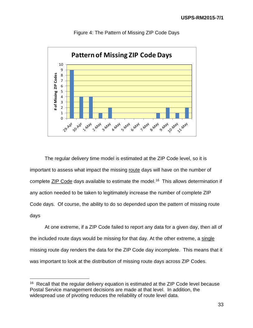
Figure 4: The Pattern of Missing ZIP Code Days

The regular delivery time model is estimated at the ZIP Code level, so it is

important to assess what impact the missing route days will have on the number of

complete ZIP Code days available to estimate the model.16 This allows determination if

any action needed to be taken to legitimately increase the number of complete ZIP

Code days. Of course, the ability to do so depended upon the pattern of missing route

days

At one extreme, if a ZIP Code failed to report any data for a given day, then all of

the included route days would be missing for that day. At the other extreme, a single

missing route day renders the data for the ZIP Code day incomplete. This means that it

was important to look at the distribution of missing route days across ZIP Codes.

16 Recall that the regular delivery equation is estimated at the ZIP Code level because Postal Service management decisions are made at that level. In addition, the widespread use of pivoting reduces the reliability of route level data.

0123456789

10

# of

Miss

ing

ZIP

Code

sPattern of Missing ZIP Code Days

USPS-RM2015-7/1

34

59.5 percent of the missing route days occurred in ZIP Codes for which no data

were reported for any routes. Nothing could be done to recover data from the missing

routes for these ZIP Code days, and they were excluded from the analysis dataset. The

remaining 40.5 percent of missing route days occurred on ZIP Code days in which

some of the routes in the affected ZIP codes were reporting data. The key issue is

how many of the routes within the ZIP Code were reporting data. If the non-reporting

routes in a ZIP Code were a small percentage of the total routes, then it may be

possible to preserve the ZIP Code day’s data by imputing collection volumes for the

missing routes. But if too many routes were missing data, then caution was

appropriate, to be sure that the collection volumes for the entire ZIP Code day did not

reflect just a few of its routes. Prudence dictated that imputation was considered only

for ZIP Code days for which at least 80 percent of the routes reported volume.

In addition, imputation for a route was done only when there were many valid

days of data reported for that route. As the following chart shows, imputation was rarely

repeated for a route, with the overwhelming majority of routes needing imputation for

just one day. However, there were six routes which apparently required many, if not all,

days of imputation. Investigation revealed that for the six routes with high numbers of

imputations, all the imputed values were zero. This is because all six routes were

“vacant” routes which had neither hours nor volume and so they actually had zero

collection volume.

For all routes that required positive-valued imputations, there were a sufficient

number of reported collection volume days so that it was legitimate to use mean values

over the days for which the route reported volume as the imputed values.

USPS-RM2015-7/1

35

Figure 5: Distribution of Imputed Volumes

Among the ZIP Code days with at least one route missing data, some had no

data reported for any routes, and were thus unusable. Other ZIP Code days had less

than 80 percent of its routes reporting data, so they were dropped from the dataset.

One ZIP Code had missing route data for each of the 12 days of the study.

Because of this persistent pattern of non-reporting, all days for this ZIP Code were

dropped from the data set, despite the fact that half of them had at least eighty percent

of routes reporting. In total, there were 125 ZIP Code days recovered through the use

of imputed volumes. Table 11 shows the structure of the collection dataset.

81

18

70 0 0 0 0 1 0 1 4

0

10

20

30

40

50

60

70

80

90

1 2 3 4 5 6 7 8 9 10 11 12

# of

Rou

tes

# of Days with Imputed Volumes

Distribution of Imputed Volumes By Route

USPS-RM2015-7/1

36

Table 11 Use of ZIP Code days in the Analysis Data Set

Total Possible Observations

Included Observations

Dropped or Missing

Observations % Missing

ZIP Code Days 3,564 3,513 51 1.4%

Because ZIP Codes with partially missing routes either had imputed values for

those missing routes or were dropped from analysis data set, “route coverage” is not an

issue. All ZIP Code days in the analysis dataset have complete coverage, in the sense

that data from all of routes were included in the ZIP Code data. In other words, all ZIP

Code days were complete.

5. Analyzing the collected data

While the regular delivery equation was estimated with ZIP Code day volumes, it

was reasonable to initially review the route day collection statistics, as they were more

familiar. The next table provides sample statistics for the individual collection volume

measures. The sample statistics suggest that carrier collection is primarily a letter

phenomenon. The median value for letters collected from customer receptacles was

76 per route per day, while the median values for flats and packages collected were

both zero. In addition, nearly all collection volume obtained by regular letter carriers (as

opposed to special purpose route carriers who sweep street letter boxes) came from

customer receptacles.

USPS-RM2015-7/1

37

Table 12 Route Day Statistics for Collection Volume Measures

Mean Median Mode C.V.

Customer Letter 139.4 76 57 1.67

Customer Flat 12.6 0 0 3.11

Customer Package 2.9 0 0 4.23

Collection Point Letter 12.0 0 0 8.62

Collection Point Flat 1.1 0 0 14.66 Collection Point Package 0.4 0 0 18.48

Container Letter 2.8 0 0 12.28

Container Flat 1.2 0 0 19.33

The distribution of collection volumes across all routes includes a relatively large

number of zero observations for flats and packages in the low end of the distribution,

and a relatively small number of extremely high-volume observations at the other end of

the distribution. In other words, many routes got very little collection mail, but a few

routes got a lot. In fact, there were a small number of routes that reported

extraordinarily high collection volumes. There were 30 route days with more than 4,000

pieces of collection mail. Those route days occur on 19 different routes in 15 ZIP

Codes.

These volumes were generally verified during the data collection process, but

because of their unusual nature they deserved another examination, as potential

outliers. To that end, the highest collection volume route days, both in terms of total

collection volume, and by shape, were individually examined. The investigation into the

outliers involved contacting the local site coordinators to verify the counts entered. On

USPS-RM2015-7/1

38

several occasions the local coordinator verified the entered count with the carrier who

collected the mail. The potential outlier was retained only if the local coordinator verified

the accuracy of the entry. If the entry could not be verified the data point was dropped

from the analysis dataset.

A number of interesting points arose through the examination process.

Most high collection volume routes were business or mixed routes. None of them were

foot routes. High collection volume days tended to occur on the same routes throughout

the sample period and they are typically created by a small number of business delivery

points. For example, a route in Indiana reported over 1,900 letters collected. This

turned out to be a business route with a few high-volume businesses. A route in

Kentucky with high daily collected package volumes counts included a lawn parts

service business that regularly sends out large numbers of packages. A route in North

Carolina with high daily flats counts included a custom fabric and gift wrap business that

regularly sends a high number of flats to customers. Because they are valid, these high-

volume observations were retained in the data set.

There was also a wide dispersion in the amount of daily collection mail volume

across ZIP Codes. The mean number of pieces collected per day per ZIP Code was

3,520. The range in collected volume was from no pieces to over 20,000 pieces. There

were three ZIP Code days with zero collection volume.

USPS-RM2015-7/1

39

Table 13 Daily ZIP Code Collection Volume

Quantile Estimate 100% Max 21,634.6

99% 14,690.3

95% 9,972.6

90% 7,749.3

75% Q3 4,862.5

50% Median 2,587.0

25% Q1 1,237.4

10% 380.0

5% 209.0

1% 43.7

0% Min 0.0

To pursue an external validation of the collection volumes produced by the field

study, one can compare the means and medians from the City Carrier Cost System in

FY2012 with the same statistics for the data collected from the field study. Table 14

indicates that there is a correspondence between the two estimates of collection

volume.

Table 14 Comparing Measures of Central Tendency For Two Different

Sets of Collection Data

Source Mean Median

Collection Volume Study 173.6 94.6

FY2012 City CCS 181.4 95.0

USPS-RM2015-7/1

40

6. Combining Collection Volumes with Delivery Volumes.

Because of good route number hygiene, collection volumes by route and ZIP

Code matched their associated DOIS delivery volumes, by route and ZIP Code for all

route days included in the study. This lead to construction of a complete volume cost

driver data set for all 3,513 ZIP Code days. The next table compares measures of

central tendency for collection and delivery volumes. Average daily delivery volume

was more than 10 times average daily collection volume.

Table 15

The SAS programs used to obtain the final analysis dataset of 3,513 observations are

contained in USPS-RM2015-7/1.

Mean MedianCollected Letters 3,193.5 2,340.9

Collected Flats 293.4 162.9

Collected Parcels 67.4 38.0

Cased Letters 2,180.2 1,656.0

Cased Flats 7,276.0 5,631.0

Parcels 423.2 318.0

DPS 30,636.9 27,717.0

FSS 2,121.4 0.0

Sequenced 4,923.6 122.0

Sample Statistics for ZIP Code Volumes

USPS-RM2015-7/1

41

D. Creation of the Analysis Data Set

Along with delivery volumes, DOIS provides daily observations on total street

time hours for all of the routes in a ZIP Code. Recall, however, that the dependent

variable in the regular delivery equation is regular delivery hours, not total street hours.

Constructing that exact dependent variable thus requires turning DOIS street hours into

regular delivery hours. In other words, the regular delivery time equation requires data

reflecting only regular delivery time, not the complete street time, so it is necessary to

subtract out the time for other activities to develop a “pure” regular delivery time.

The calculation starts with recognition that total daily DOIS street time is the sum

of daily regular delivery time and daily allied street time. Allied street time includes

activities that carriers perform other than the regular delivery of letters and flats. Table

16 presents the breakout of average daily allied street time, as provided by the route

evaluation (Form 3999) data.

USPS-RM2015-7/1

42

Table 16

Note that the allied activities do not directly depend upon the delivered letter and

flat or collection volumes on individual routes.17 This means that the allied activities are

not determined by the daily volumes used in estimating the delivery time equation.

Consequently, each route’s regular delivery time can be calculated by taking its total

street time and subtracting its allied street time. This calculation can be made with the

17 Recall that the collection volumes in the regular delivery activity are the volumes city letter route carriers collect from customer receptacles. The time for collections from street letter boxes is in a separate cost pool and depends upon separately measured volumes. In other words, the allied activity “Collect from Street Letter Boxes” does not directly depend upon the volumes measured in the collection volume study.

Hours Proportion of Allied Time

Relay 0.21 12.6%Travel To 0.13 7.7%Travel From 0.14 8.6%Vehicle Load 0.22 13.0%Vehicle Unload 0.1 5.7%Travel Within 0.16 9.6%Accountable Time 0.08 5.0%Parcel Time 0.16 9.7%Collect SLB 0.01 0.6%Non Recurring 0.12 7.1%Break 0.23 13.8%Deadhead 0.01 0.7%Personal 0.08 4.9%Customer 0.01 0.4%Gas Vehicle 0.01 0.6%Total Allied 1.68 100.0%

Average Daily Allied Street Times

USPS-RM2015-7/1

43

total street time data from the DOIS database and the allied time data from the route

evaluation (Form 3999) database.

Subtracting this route evaluation measure of allied street time from the total

street time produces daily regular delivery time. But the route evaluation measure of

allied time is just a single measure for each route, and does not vary from day-to-day,

whereas the DOIS data provides daily street time. Because this measure of allied time

does not vary from day-to-day, it is important to investigate the econometric implications

of subtracting a route-specific allied time from each route-day's total street time.

The investigation starts with defining the mathematical relationship between total

street time, regular delivery time, and allied time. Note that in the following equation, "t"

indexes the days over which data were collected and "i' indexes the routes for which

data were collected. Define “ST” to be total street time, “DT” to be regular delivery time

and “AT” to be allied street time. The first step is to express the relationship among

these measures of street time as:

𝐷𝐷𝐷𝐷𝑖𝑖𝑖𝑖 = 𝐷𝐷𝐷𝐷𝑖𝑖𝑖𝑖 + 𝐴𝐴𝐷𝐷𝑖𝑖𝑖𝑖 Rearranging this equation provides an expression for regular delivery time:

𝐷𝐷𝐷𝐷𝑖𝑖𝑖𝑖 = 𝐷𝐷𝐷𝐷𝑖𝑖𝑖𝑖 − 𝐴𝐴𝐷𝐷𝑖𝑖𝑖𝑖

As explained above, the route evaluation data does not contain measures of

allied street time by day. Rather, it measures the systematic allied time for each route,

which is defined as: 𝐴𝐴𝐷𝐷�𝑖𝑖𝑖𝑖. On any given day, the actual allied time may differ from the

systematic allied time because of random factors, such as more or less traffic on the

USPS-RM2015-7/1

44

route, or a variation in a carrier’s personal needs time. This means an expression for

daily allied time can be thus written as:

𝐴𝐴𝐷𝐷𝑖𝑖𝑖𝑖 = 𝐴𝐴𝐷𝐷� 𝑖𝑖𝑖𝑖 + 𝜇𝜇𝑖𝑖𝑖𝑖

Note that 𝜇𝜇𝑖𝑖𝑖𝑖 is the unobserved day-to-day variation in allied time on a route.

Substituting this formulation for allied time into the regular delivery time definition

provides an expression for regular delivery time as a function of what is observed (total

street time and systematic allied time) and what is not observed (random daily

variations in allied time):

𝐷𝐷𝐷𝐷𝑖𝑖𝑖𝑖 = 𝐷𝐷𝐷𝐷𝑖𝑖𝑖𝑖 − � 𝐴𝐴𝐷𝐷�𝑖𝑖𝑖𝑖 + 𝜇𝜇𝑖𝑖𝑖𝑖�

This formulation permits investigation of the econometric implications of using the

constructed measure of delivery time for estimating the regular delivery time equation.

The regular delivery time equation specifies that delivery time is a function of the cost

drivers (Xj) and characteristic variables (θi):

𝐷𝐷𝐷𝐷𝑖𝑖𝑖𝑖 = 𝛼𝛼0 + �𝛽𝛽𝑗𝑗𝑋𝑋𝑗𝑗𝑖𝑖𝑖𝑖 + 𝑛𝑛

𝑗𝑗=1

�𝛾𝛾𝑘𝑘θ𝑘𝑘𝑖𝑖𝑖𝑖 + 𝜀𝜀𝑖𝑖𝑖𝑖 𝑚𝑚

𝑘𝑘=1

Substituting the expression for regular delivery time yields:

𝐷𝐷𝐷𝐷𝑖𝑖𝑖𝑖 − � 𝐴𝐴𝐷𝐷�𝑖𝑖𝑖𝑖 + 𝜇𝜇𝑖𝑖𝑖𝑖� = 𝛼𝛼0 + �𝛽𝛽𝑗𝑗𝑋𝑋𝑗𝑗𝑖𝑖𝑖𝑖 + 𝑛𝑛

𝑗𝑗=1

�𝛾𝛾𝑘𝑘θ𝑘𝑘𝑖𝑖𝑖𝑖 + 𝜀𝜀𝑖𝑖𝑖𝑖 𝑚𝑚

𝑘𝑘=1

or:

USPS-RM2015-7/1

45

𝐷𝐷𝐷𝐷�𝑖𝑖𝑖𝑖 = 𝛼𝛼0 + �𝛽𝛽𝑗𝑗𝑋𝑋𝑗𝑗𝑖𝑖𝑖𝑖 + 𝑛𝑛

𝑗𝑗=1

�𝛾𝛾𝑘𝑘θ𝑘𝑘𝑖𝑖𝑖𝑖 + 𝜂𝜂𝑖𝑖𝑖𝑖 𝑚𝑚

𝑘𝑘=1

where:

𝐷𝐷𝐷𝐷�𝑖𝑖𝑖𝑖 = 𝐷𝐷𝐷𝐷𝑖𝑖𝑖𝑖 − 𝐴𝐴𝐷𝐷�𝑖𝑖𝑖𝑖

𝜂𝜂𝑖𝑖𝑖𝑖 = 𝜀𝜀𝑖𝑖𝑖𝑖 + 𝜇𝜇𝑖𝑖𝑖𝑖

This specification reveals that the estimated coefficients for the cost drivers and

characteristic variables are unbiased and consistent. The "true" dependent variable

already has a stochastic term (𝜀𝜀𝑖𝑖𝑖𝑖) associated with it and adding another one does not

affect the relationship between the dependent variable and the independent variables.

To see this, observe that the expected value of the composite stochastic term is just the

sum of the expected values of the individual stochastic terms:

𝑆𝑆(𝜂𝜂𝑖𝑖𝑖𝑖) = 𝑆𝑆(𝜀𝜀𝑖𝑖𝑖𝑖 + 𝜇𝜇𝑖𝑖𝑖𝑖) = 𝑆𝑆(𝜀𝜀𝑖𝑖𝑖𝑖 ) + 𝑆𝑆(𝜇𝜇𝑖𝑖𝑖𝑖) = 0.

In addition, the composite stochastic term is not correlated with the right-hand-side

variables in the regression:

𝑆𝑆�𝜂𝜂𝑖𝑖𝑖𝑖,𝑋𝑋𝑗𝑗𝑖𝑖𝑖𝑖� = 𝑆𝑆(𝜀𝜀𝑖𝑖𝑖𝑖 𝑋𝑋𝑗𝑗𝑖𝑖𝑖𝑖 + 𝜇𝜇𝑖𝑖𝑖𝑖𝑋𝑋𝑗𝑗𝑖𝑖𝑖𝑖) = 𝑆𝑆(𝜀𝜀𝑖𝑖𝑖𝑖 𝑋𝑋𝑗𝑗𝑖𝑖𝑖𝑖) + 𝑆𝑆�𝜇𝜇𝑖𝑖𝑖𝑖𝑋𝑋𝑗𝑗𝑖𝑖𝑖𝑖� = 0.

On the other hand, the estimated coefficients are likely to be inefficient. The size

of the estimated equation’s stochastic term is likely to be larger with the constructed

measure of delivery time and a larger stochastic term leads to a larger variance for the

estimated coefficients. In the true model:

USPS-RM2015-7/1

46

𝐶𝐶��̂�𝛽𝑖𝑖� = 𝜎𝜎𝜀𝜀2

(∑𝑋𝑋𝑖𝑖 − 𝑋𝑋�)2 In the constructed dependent variable case:

𝐶𝐶��̂�𝛽𝑖𝑖� = 𝜎𝜎𝜂𝜂2

(∑𝑋𝑋𝑖𝑖 − 𝑋𝑋�)2 = 𝜎𝜎𝜀𝜀2 + 𝜎𝜎𝜇𝜇2

(∑𝑋𝑋𝑖𝑖 − 𝑋𝑋�)2

Inefficiency means that the standard errors for the estimated coefficients will be larger

than they would be without the construction. Theoretically, larger standard errors could

affect inference and make it more difficult to perform statistical tests on the coefficients.

Such an inefficiency problem can be solved by having a large data set so the standard

errors of the estimated coefficients are small to begin with. Then a modest degree of

inefficiency does not affect inference. With a large dataset, reliable statistical inference

is still possible even with a constructed dependent variable. This is the case for the

estimation of the regular delivery equation. The analysis data set includes nearly 3,500

ZIP Code-day observations and is large enough to produce relatively small standard

errors. Results from estimation of the equation, presented below, demonstrate that the

potential inefficiency associated with a constructed dependent variable did not create a

problem in practice and reliable statistical inference could be made.

To construct the regular delivery time variable, the route evaluation data (the

Form 3999 data set) that includes allied time must be merged with the DOIS/CV data

set which includes street time, volumes, and delivery points. The Form 3999 data set

has over 140,000 route observations as it has one observation for each route in the

USPS-RM2015-7/1

47

country. The DOIS/CV data set has 71,933 route day observations covering the 6,066

individual routes in the study. Merger of the two data sets thus requires matching the

allied time from the route evaluation data set to each of the corresponding routes in the

DOIS/CV data set.

Initial efforts at matching the two data sets revealed that there were just 21 of the

6,066 routes (in 10 different ZIP Codes) that could not be matched. The failure to match

occurred because the route evaluation data set did not include a measure of allied time

for those routes. If this situation cannot be remedied, it will lead to 120 ZIP Code days

(10 ZIP Codes times 12 days) with incomplete data. However, investigation of the ZIP

Codes with missing Form 3999 data shows that it is usually just one route in each ZIP

with missing data.

The next table presents the ZIP Codes that have routes in the DOIS/CV data set

without a corresponding value for allied time in the route evaluation data. It also

presents the number of non-match routes in each ZIP Code along with the total number

of routes in those ZIP Codes.

USPS-RM2015-7/1

48

Seven of the ten affected ZIP Codes have just one route with missing allied time data

and eight of the ten affected ZIP Codes have less than twenty percent of their routes

with missing data. In those ZIP Codes in which there are only one or two routes with

missing allied time, the missing allied time can be imputed by using the average allied

time over the remaining routes in that ZIP Code, that do have a measure of allied time.

The imputed values for the missing routes are given in Table 18.

Table 17 Identifying the ZIP Codes with Missing Form 3999 Data

Masked ZIP Code

Routes with Missing

Allied Time

Total Number of

Routes % Missing

Routes 85918 1 16 6.3%

32732 1 6 16.7%

60966 1 8 12.5%

35323 2 39 5.1%

15092 1 31 3.2%

94118 5 25 20.0%

60333 1 23 4.3%

98915 7 34 20.6%

64921 1 23 4.3%

20340 1 31 3.2%

USPS-RM2015-7/1

49

Table 18

Imputed Allied Times in Selected ZIP Codes

Masked ZIP Code Route

Imputed Allied Time

85918 C071 2.31

32732 C016 1.16

60966 C032 1.91

35323 C049 2.02

35323 C050 2.02

15092 C095 1.67

60333 C080 1.63

64921 C076 2.88

20340 C051 2.49 By imputing allied time for these 9 routes, an additional 96 ZIP Code days were

recovered. This means that there just two (masked) ZIP Codes, 94118 and 98915 with

incomplete data. Because of the number of missing routes, these ZIP Codes were

dropped from the analysis data set. The analysis data set thus contains 3,489 out of

3,513 possible complete ZIP Code days. This represents 99.3 percent of the possible

ZIP Code days. It important to note that the included ZIP Code observations are

complete, in the sense that there are no missing routes on any of the ZIP Code days.

The last step in building the analysis data set is to construct the relevant values

for the characteristic variables. As explained above, there are three characteristic

variables included in the econometric equation, a delivery technology indicator, the

USPS-RM2015-7/1

50

proportion of business addresses and the square miles per delivery point in the ZIP

Code.

The delivery technology indicator is based upon the delivery technology used on

the routes within the ZIP Code. The following table presents the distribution of the

6,066 routes in the sample across these five types.

Recall that the delivery mode indicator is assigned a value of zero if it is a

curbline or dismount route (driving route) and a value of one if it is a foot, park and loop,

or other route (walking route). The technology indicator is the percentage of walking

routes in the ZIP Code and has a range from zero through one. The average value for

this technology indicator is 0.56.

One could consider defining a ZIP Code’s delivery technology through using

delivery point data as opposed to route type data. For example, one could consider

Table 19

Distribution of Routes by Delivery Technology

Frequency Proportion

Curbline 1,392 23.0%

Dismount 1,181 19.5%

Foot 347 5.7%

Park and Loop 3,138 51.7%

Other 8 0.1%

USPS-RM2015-7/1

51

door delivery points and perhaps central delivery points as "walking" delivery points and

curbline and perhaps CBU delivery points as “driving” delivery points. However, such

an approach is less likely to provide a clear demarcation of delivery technology. This is

because individual types of delivery points can be served with either a driving

technology or a walking technology. Door delivery points are served by walking on foot

or park and loop routes, but they are also served by driving on curbline and dismount

routes. Similarly CBU delivery points are served by both walking and driving depending

upon the route on which they occur.

This heterogeneity is highlighted in the Table 20, which presents a distribution of

the sampled delivery points, by type, across route types.

Table 20

Distribution of Delivery Points by Route Type

Route Type

Curbline Dismount Foot

Park and Loop Other

Del

iver

y Po

int

Type

Door 11.5% 29.9% 34.1% 66.2% 42.4%

Curb 62.2% 12.2% 0.0% 6.6% 1.5%

CBU 15.0% 24.1% 2.6% 7.4% 9.9%

Central 11.2% 33.8% 63.4% 19.8% 46.2%

The next characteristic variable to controls for the possibility that business

delivery points may require a different amount of time than residential delivery points for

the same amount of volume. This variable is calculated as the percentage of business

USPS-RM2015-7/1

52

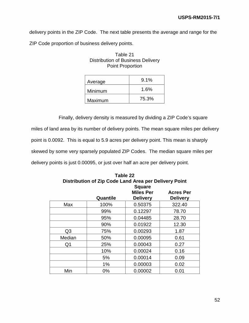
delivery points in the ZIP Code. The next table presents the average and range for the

ZIP Code proportion of business delivery points.

Table 21 Distribution of Business Delivery

Point Proportion

Average 9.1%

Minimum 1.6%

Maximum 75.3%

Finally, delivery density is measured by dividing a ZIP Code’s square

miles of land area by its number of delivery points. The mean square miles per delivery

point is 0.0092. This is equal to 5.9 acres per delivery point. This mean is sharply

skewed by some very sparsely populated ZIP Codes. The median square miles per

delivery points is just 0.00095, or just over half an acre per delivery point.

Table 22 Distribution of Zip Code Land Area per Delivery Point

Quantile

Square Miles Per Delivery

Acres Per Delivery

Max 100% 0.50375 322.40 99% 0.12297 78.70 95% 0.04485 28.70 90% 0.01922 12.30

Q3 75% 0.00293 1.87 Median 50% 0.00095 0.61

Q1 25% 0.00043 0.27 10% 0.00024 0.16 5% 0.00014 0.09 1% 0.00003 0.02

Min 0% 0.00002 0.01

USPS-RM2015-7/1

53

The next table presents the sample statistics, by ZIP Code day for variables included in

the econometric equation.

Table 23 Sample Statistics for Included Variables

Variable Mean Std. Deviation Minimum Maximum

Regular Delivery Hours 94.2 50.1 0.5 304.7

DPS 30,600 19,980 0 168,931

Cased Mail 9,443 7,040 155 57,363

Sequenced 4,898 7,507 0 58,255

FSS 2,138 4,576 0 35,785

Collection 3,547 3,262 0 21,216

Delivery Points 12,298 6,425 531 30,367

Delivery Mode 0.56 0.37 0 1.00

Miles per DP 0.01 0.03 0.00002 0.50

Ratio of Business DPs 0.09 0.07 0.02 0.75

E. Estimation of the Model and Discussion of the Results

The functional form of the delivery equation is quadratic. It has cross products

among the cost drivers, but not the characteristic variables. This means it has 34

estimated coefficients, including the intercept. Note that there are three sets of

coefficients to review. The first set consists of the linear and quadratic terms for the

cost drivers - the volume variables and delivery points. These variables are primarily

responsible for causing delivery time and are the most important in determining the

USPS-RM2015-7/1

54

estimated variabilities. The second set represents the cross products among the cost

drivers. These variables account for the fact that delivery time is different for a group of

products than it is if those products are delivered individually. For example, under

economies of scope, it take less time to deliver two products at the same time than it

does to deliver both of the products individually. The third set includes the coefficients

for the characteristic variables which measure the impact of the delivery environment on

delivery time.

The complete estimation results are provided in USPS-RM2015-7/1. A summary

of the results is provided in the next table. Before reviewing of the results, it is important

to acknowledge two potential econometric problems. The estimation of an econometric

equation relies upon a set of assumptions that underlie important qualities of the

estimated coefficients. When these assumptions are violated, the possibility of spurious

inference arises, so it makes sense to check if the model and data match up well with

the assumptions. Two assumptions that are often violated are the assumptions of

homoscedastic disturbance terms and orthogonal right-hand-side variables. When

those assumptions do not hold, the econometric equation may be subject to

heteroscedasticity and/or multicollinearity.

Because these problems had been detected in previously-estimated regular

delivery equations, it is prudent to investigate them this time. Such an investigation

includes understanding how the problems arise, determining how they can be detected,

and, if necessary, addressing how they can be corrected. Heteroscedasticity will be

investigated before the initial results are presented and, if appears to be present,

multicollinearity will be investigated afterward.

USPS-RM2015-7/1

55

One underlying assumption of the regression model is that the variance of the

stochastic terms is constant around the regression line. Consider the following

regression equation in which y is the dependent variable, x is the independent variable,

and ε is the stochastic, or disturbance, term:

𝑦𝑦𝑖𝑖 = 𝛼𝛼 + 𝛽𝛽 𝑥𝑥𝑖𝑖 + 𝜀𝜀𝑖𝑖 . If the variance of the disturbance terms is constant around the regression line, then the

distribution of the εi around the regression will be the same, regardless of the position

on the regression line. This is illustrated in the Figure X which shows the distribution of

the disturbance at various points on the regression line.

Figure 6: Distribution of Disturbances around a Regression Equation

Moreover, if the variance is constant around the regression line, then a plot of the

residuals against the predict values (which are on the regression line) should show the

y

x

USPS-RM2015-7/1

56

same spread at all predicted values for the dependent variable This can be investigated

by plotting the residuals (e) against the predicted values (y hat). The residuals in the

following plot are homoscedastic:

Figure 7: Homoscedastic Residuals

If the residuals show a pattern of increasing or decreasing at different places

along regression line, then it is likely that the variance of the stochastic term is

heteroscedastic. The most common form of heteroscedasticity comes from

increasing variance as the size of the dependent variable increases. The following

plot shows an example of a heteroscedastic disturbance term.

e

Y hat

USPS-RM2015-7/1

57

Figure 8: Heteroscedastic Residuals

Because it relates just to the variance of the error terms, heteroscedasticity has

no impact on the estimated coefficients.18 The ordinary least squares coefficients

remain unbiased estimators of the true regression coefficients.

On the other hand, the estimated standard errors of those coefficients are

generally biased downward. This means that standard hypothesis tests are not valid.

The downward bias comes from the fact that the least squares procedure minimizes the

sum of the squared residuals. Under heteroscedasticity, the least squares procedure

puts more weight on the observations with large variances. But those observations

18 The appearance of severe heteroscedasticity could be the reflection of a more serious problem with the model, such as a miss-specified model. If so, the underlying problem could be affecting the estimated coefficients even though the heteroscedasticity is not. This should be kept in mind when investigating heteroscedasticity.

e

Y hat

USPS-RM2015-7/1

58

should actually have the smallest weights because they contain the least real

information about the model compared to their amount of "noise." As a result, the

estimated standard errors are smaller than the actual ones.

There are a number of methods of detecting heteroscedasticity. The first is

"ocular inspection," looking at the residuals. A plot of the residuals against the

predicted values from a regression may reflect a pattern in variance. Below is the plot

of the residuals against the predicted values from the regular delivery equation. The

plot suggests that the variance of the residuals increases as the regular delivery time of

the ZIP Code days increase.

Figure 9: Residuals Plotted Against Predicted Values from Regular Delivery Equation

Plot of resid*pv. Legend: A = 1 obs, B = 2 obs, etc. ‚ ‚ 150 ˆ ‚ ‚ ‚ A ‚ A ‚ B ‚ A A A 100 ˆ A ‚ B ‚ A ‚ A ‚ A A A A A ‚ A A A AA A BA A A R ‚ A DBDABA ABBAA B A A e 50 ˆ BACA D ACACC s ‚ AA BA BABBCBABBABADAA AA A A i ‚ ABA A BA DBA AEF CDAEAAAAAAA ABA BAAA A d ‚ ACA BC AAAECBDCC FFFFCADA BACDC BABA A A A u ‚ F A BEBDDDCBADHELKICKICJEFDECBCAABFAAD ABB A A a ‚ JJOABC ACEGDBDAADLEIEEHQGDACNGKOQHTHICIDDGCDBFAB DCDD B l ‚ BGFBNMMPPHLODHNNGNPPLMHPEJHIGFGKMJMSRKMHJFIKDEFCEBDDCA BCAB A 0 ˆ JIZGHSTYSZQHZVWZZXXQXXRRRKGKKMNKGQJJMKEHHJCFKBBFBBBABABA A ‚ BKRILHIOSSKVPYYYZMSRSYVPZSNLKINJONIGMIGGIHEHGCCB A A A A ‚ FA BB DDFBJSMWRMRSQNRRWLHQKNFIICJFHHDDFDAD C C A A ‚ A BBABIICHNIGKLICGGIFLEDIICFEEFDEABDEC B AA ‚ AAAACAB BABBAAEBAHDDFEHCCJABDBAC BCADBAAAA ‚ A BBAECCCBABCFECDCACB B A A BA A ‚ A A BA BBA AB CA A A -50 ˆ A AA AA AAC A A ‚ A A AABAA ‚ A A A AA ‚ A A A ‚ ‚ ‚ A -100 ˆ ‚ Šƒˆƒƒƒƒƒƒƒƒƒƒƒƒƒˆƒƒƒƒƒƒƒƒƒƒƒƒƒˆƒƒƒƒƒƒƒƒƒƒƒƒƒˆƒƒƒƒƒƒƒƒƒƒƒƒƒˆƒƒƒƒƒƒƒƒƒƒƒƒƒˆƒƒƒƒƒƒƒƒƒƒƒƒƒˆƒƒ -50 0 50 100 150 200 250 Predicted Value of delivery_hrs

USPS-RM2015-7/1

59

However, the plot is not definitive, so it is useful to have some empirical tests for

heteroscedasticity. A first test is called the Breusch-Pagan (BP) test. This test is based

upon the idea that if the residuals have constant variance, then the variance should not

vary with any of the right-hand-side variables. The BP test is based upon an auxiliary

regression in which the squared residuals are regressed upon the model's right-hand-

side variables:

𝜀𝜀�̂�𝑖2 = 𝛾𝛾0 + �𝛾𝛾𝑘𝑘𝑥𝑥𝑗𝑗𝑖𝑖 𝑘𝑘

𝑗𝑗=1

+ 𝜐𝜐𝑖𝑖 .

Under the null hypothesis of homoscedasticity, the γk will all equal zero and the

equation will have not have any explanatory power. The null hypothesis is tested by

constructing the following test statistic, nR2, which has a chi-square distribution with k

degrees of freedom. In the case of the regular delivery equation, the chi-square critical

value from the auxiliary regression has 26 degrees of freedom:

𝑛𝑛𝐵𝐵2 ~ 𝜒𝜒26,.052

The White test is similar to the BP test, except that it uses not only the right-

hand-side variables but also their squares and cross products. In the case of the

regular delivery equation, the White test has 305 degrees of freedom. It has the same

calculated test statistic, nR2, and also has a chi-squared distribution.

As the following table shows, both tests indicate rejection of the null hypothesis

of homoscedasticity in favor of the alternative hypothesis of heteroscedasticity.

USPS-RM2015-7/1

60

Table 24 Testing for Heteroscedasticity

Test Bruesch-Pagan White

Degrees of Freedom 26 305

Test Statistic 869.9 1865

Critical Value 38.85 124.34

Result Reject H0 Reject H0

Given that the two tests indicate the presence of heteroscedasticity, the issue

now becomes what to do about it. Because the estimated coefficients are unbiased,

heteroscedasticity can be ignored if one is not concerned with hypothesis testing.19

That is not the case for the regular delivery equation, as it is important to test the

significance of the regression coefficients that will be used to calculate the variabilities.

Thus, it is important to correct for heteroscedasticity.

There are two primary ways of correcting for heteroscedasticity: using weighted

least squares and using robust standard errors. Both were considered for correcting the

regular delivery equation. Suppose that the form of the heteroscedasticity is known. In

this situation, start again with the simple model:

𝑦𝑦𝑖𝑖 = 𝛼𝛼 + 𝛽𝛽 𝑥𝑥𝑖𝑖 + 𝜀𝜀𝑖𝑖 . 19 It is at this point one also assesses the model to investigate whether heteroscedasticity is reflecting a larger problem. To do so, one asks if the appropriate right-hand-side variables are included in the equation, if the overall fit of the equation is acceptable, and if there is an understandable reason why heteroscedastic disturbances could arise. The answers to these questions for the regular delivery equation are all affirmative and indicate that heteroscedasticity is not reflecting a deeper problem.

USPS-RM2015-7/1

61

The heteroscedasticity is assumed to be of the following form:

𝐶𝐶(𝜀𝜀𝑖𝑖) = 𝜎𝜎2𝑥𝑥𝑖𝑖2. In other words the variance of the stochastic term increases with the right-hand-side

variable. Given this form, the original model can be divided by 𝑥𝑥𝑖𝑖: 20

𝑦𝑦𝑖𝑖𝑥𝑥𝑖𝑖

= 𝛼𝛼𝑥𝑥𝑖𝑖

+ 𝛽𝛽 + 𝜀𝜀𝑖𝑖𝑥𝑥𝑖𝑖

.

The variance of the transformed error term is homoscedastic:

𝐶𝐶 � 𝜀𝜀𝑖𝑖𝑥𝑥𝑖𝑖� =

𝜎𝜎2𝑥𝑥𝑖𝑖2

𝑥𝑥𝑖𝑖2 = 𝜎𝜎2.

The problem with this approach is that it requires knowing the form of

heteroscedasticity, which is not known for the regular delivery equation. This means

that the model's coefficient estimates could be biased by using the wrong variable for

the transformation. When the form of the heteroscedasticity is not known, it is

appropriate to use the other method of correction: robust standard errors.

Robust standard errors can be applied when the variance structure is unknown.

In this approach, ordinary least squares are used to estimate the coefficients, but new

standard errors that allow for heteroscedasticity are calculated. Under

heteroscedasticity, the OLS standard errors are given by:

20 This is called "weighted" least squares because it is the same as multiplying each observation by a weight of

1𝑥𝑥𝑖𝑖

.

USPS-RM2015-7/1

62

𝐶𝐶(𝛽𝛽) = ∑ [(𝑥𝑥𝑖𝑖 − �̅�𝑥)2𝜎𝜎𝑖𝑖2]𝑁𝑁𝑖𝑖=1

[∑ (𝑥𝑥𝑖𝑖 − �̅�𝑥)2𝑁𝑁𝑖𝑖=1 ]2 .

This formula depends upon the values for the heteroscedastic errors, the 𝜎𝜎𝑖𝑖2. However,

they are unknown, and are replaced with consistent estimates, the squared residuals:

𝐶𝐶(𝛽𝛽)𝑟𝑟𝑟𝑟𝑟𝑟𝑟𝑟𝑟𝑟𝑖𝑖 = ∑ [(𝑥𝑥𝑖𝑖 − �̅�𝑥)2𝑒𝑒𝑖𝑖2]𝑁𝑁𝑖𝑖=1 / (𝑁𝑁 − 𝐾𝐾)

[∑ (𝑥𝑥𝑖𝑖 − �̅�𝑥)2𝑁𝑁𝑖𝑖=1 ]2 / 𝑁𝑁

.

Table 25 presents the full set of OLS and heteroscedasticity-consistent (robust)

standard errors for the full regular delivery model. The table shows the reduction in

standard errors and t-tests that arises due to heteroscedasticity. In most cases, the t-

tests are sufficiently large, even under OLS, to reject the null hypothesis of a zero

coefficient. This reflects the underlying strength of the model and suggests that

heteroscedasticity is not a severe problem.

USPS-RM2015-7/1

63

Standard StandardError t Value Error t Value

INTERCEPT 1.694 -10.21 1.39726 -12.38DPS 1.01E-04 4.87 1.23E-04 4.01DPS2 1.16E-09 -6.85 1.84E-09 -4.30CM 2.36E-04 3.28 3.28E-04 2.36CM2 5.66E-09 -3.48 6.82E-09 -2.89SEQ 1.53E-04 5.49 1.69E-04 4.98SEQ2 3.74E-09 -6.77 4.01E-09 -6.30FSS 3.02E-04 9.99 3.26E-04 9.25FSS2 1.11E-08 -2.51 1.30E-08 -2.14CV 4.31E-04 2.73 5.16E-04 2.29CV2 2.04E-08 -3.56 2.56E-08 -2.85DP 2.90E-04 23.56 2.91E-04 23.50DP2 1.41E-08 -9.29 1.64E-08 -8.00DPS*CM 4.34E-09 5.07 7.62E-09 2.89DPS*SEQ 3.41E-09 1.21 5.06E-09 0.81DPS*FSS 5.60E-09 1.97 7.73E-09 1.43DPS*CV 8.73E-09 -7.36 1.31E-08 -4.90DPS*DP 6.90E-09 6.41 1.02E-08 4.35CM*SEQ 7.98E-09 0.13 1.12E-08 0.09CM*FSS 1.54E-08 -1.48 2.06E-08 -1.11CM*CV 1.85E-08 6.01 2.86E-08 3.88CM*DP 1.51E-08 -3.72 2.17E-08 -2.59SEQ*FSS 9.98E-09 1.15 1.25E-08 0.92SEQ*CV 1.33E-08 -2.24 1.78E-08 -1.67SEQ*DP 9.61E-09 0.62 1.14E-08 0.52FSS*CV 2.47E-08 4.79 3.15E-08 3.76FSS*PD 1.81E-08 -6.81 2.37E-08 -5.21CV*DP 2.64E-08 5.36 3.62E-08 3.91DM 3.508 12.80 3.095 14.51DM2 3.401 -7.90 3.187 -8.42MPDP 22.768 3.11 11.826 5.99MPDP2 50.699 -2.38 20.132 -5.98BR 11.901 -3.48 10.31 -4.01BR2 20.021 2.34 15.39 3.05

Variable

Ordinary Least Squares Heteroscedasticity Consistent

Comparing OLS and HC Standard Errors & T-testsTable 25

USPS-RM2015-7/1

64

An example of why it can be important to correct for heteroscedasticity is given

by the coefficient on the cross product between sequenced mail and collection mail.

The OLS t-statistic for that cross product is -2.24 and the HCSE is -1.67. Thus, under

OLS it would be considered statistically significant when it is not. In addition, the fact

that so many estimated coefficients are statistically significant indicates that potential

concerns about inefficiency arising from constructing the dependent variable are not

material in practice. Table 26 presents a summary of the results of estimating the

regular delivery equation.

USPS-RM2015-7/1

65

Variable Estimated Coefficient H.C. t statisticINTERCEPT -17.30 -12.38DPS 1.77 4.01DPS2 -0.00003 -4.30CM 2.78 2.36CM2 -0.00007 -2.89SEQ 3.02 4.98SEQ2 -0.00009 -6.30FSS 10.84 9.25FSS2 -0.00010 -2.14CV 4.25 2.29CV2 -0.00026 -2.85DP 24.62 23.50DP2 -0.00047 -8.00DPS*CM 0.00008 2.89DPS*SEQ 0.00001 0.81DPS*FSS 0.00004 1.43DPS*CV -0.00023 -4.90DPS*DP 0.00016 4.35CM*SEQ 0.00000 0.09CM*FSS -0.00008 -1.11CM*CV 0.00040 3.88CM*DP -0.00020 -2.59SEQ*FSS 0.00004 0.92SEQ*CV -0.00011 -1.67SEQ*DP 0.00002 0.52FSS*CV 0.00043 3.76FSS*PD -0.00044 -5.21CV*DP 0.00051 3.91DM 44.91 14.51DM2 -26.85 -8.42MPDP 70.82 5.99MPDP2 -120.47 -5.98BR -41.38 -4.01BR2 46.87 3.05R2 0.8576# of Obs. 3485Cost driver coefficients are in seconds; characteristic variable coefficients are in hours.

Initial Estimation of the Regular Delivery Time EquationTable 26

USPS-RM2015-7/1

66

In general, the model fits well, with a high R2 and most coefficients being

statistically significant. All of the cost driver coefficients have the expected signs. The

first-order terms are positive and the second order terms are negative. The relationship

between delivery time and the cost drivers is illustrated in Figure 10.

Figure 10: Delivery Time Function under Economies of Density

The figure shows that delivery time per piece falls as the number of pieces

delivered rises, but that effect tapers off as volume gets large. This is consistent with

economies of density in delivery.

The signs on the estimated coefficients for the characteristic variables are all as

expected. As a ZIP Code becomes a more "walking" ZIP Code, keeping volume and

number of delivery points constant, delivery time rises. Similarly, as the miles per

delivery point increase, so does delivery time. As the percentage of business delivery

Volume

Delivery Time

USPS-RM2015-7/1

67

points rises, delivery time falls. In addition, in all three cases, the second order term is

of the opposite sign, meaning that the effect of the characteristic flattens out as it gets

larger. Finally, no variables have to be dropped to get sensible results.

The variabilities implied by this regular delivery equation can be derived directly

from the estimated coefficients according to the following formula:

)V(DTV

VDT i

iiV,DT ∂

∂=λ ,

where )V(DT is the predicted value for delivery time at the mean values for the

volumes, delivery points and density. The variabilities and marginal times for regular

delivery are given in the next table. There are two factors that go into the variability: the

marginal time per piece and the amount of volume in the cost driver. If two shapes

have the same marginal time but one has twice the volume of the other, then the larger-

volume shape will have a variability twice the size of the smaller-volume shape. This is

why the DPS variability is so high and why the cased mail variability is double the

sequenced variability. The overall variability with respect to all volume is just the sum of

the individual variabilities. In this instance, the overall variability is 36.1 percent.

Table 27 Variabilities and Marginal Times Produced by the

Regular Delivery Equation

Cost Driver Variability Marginal

Time DPS 16.7% 2.07

Cased Mail 6.6% 2.64

Sequenced 3.4% 2.59

FSS 4.0% 7.12

Collection 5.4% 5.72

USPS-RM2015-7/1

68

All but seven of the 34 estimated coefficients are statistically significant at the

95% level, even accounting for heteroscedasticity. This is an important result because

a major symptom of multicollinearity is inflated standard errors and thus, low t-statistics.

For example, the full model in Docket No. R2005-1 had low t-statistics for 18 of 35

coefficients.21 The fact that so many of the estimated coefficients are statistically

significant in the current work is a result of nearly doubling the size of the data set used

to estimate the equation.22

Multicollinearity (which is sometimes just called collinearity) is a problem that

arises when the right-hand-side variables in a regression are correlated with one

another. When this occurs, it may be difficult to accurately identify the separate effects

of each of the individual variables in the model.

Multicollinearity is a data problem, not a statistical problem. However, it can lead

to statistical problems and that is why it should be evaluated. Multicollinearity leads to

additional noise in the estimation of a model's parameters. If a parameter does not start

out with a large ratio of useful information to statistical noise,23 then the additional noise

created by multicollinearity could lead to the mis-estimation of the parameter.

Because it is a problem that exists among the right-hand-side variables,

multicollinearity does not affect the overall ability of the model to capture the relationship 21 See, “Testimony of Michael D. Bradley on Behalf of the United States Postal Service,” USPS-T-14, Docket No. R2005-1. 22 When the regular delivery equation was previously estimated, the data set included 1,545 ZIP Code days. The current data set has 3,485 observations. See, “Testimony of Michael D. Bradley on Behalf of the United States Postal Service,” USPS-T-14, Docket No. R2005-1. 23 This could occur if there is not much variation in the values for a right-hand-side variable in a data set. Then it may be difficult to infer the true relationship between that variable and the dependent variable.

USPS-RM2015-7/1

69

between the dependent and independent variables. This is why a model can have an

outstanding overall goodness of fit even though many individual estimated coefficients

are not statistically differentiable from zero.

The primary symptom of multicollinearity is inflated standard errors, leading to

imprecisely estimated coefficients accompanied by a high R2 value. In extreme cases,

multicollinearity can lead to parameter instability in the sense that relatively modest

changes in model specification can lead to major changes in the values of the estimated

coefficients; they can even switch sign.

Multicollinearity is very much a problem of degree. It can exist and reduce, to a

certain extent, the accuracy of coefficient estimation without causing any specific harm

to the estimation of the model. For example, if the relationship between the dependent

variable and the independent variable is robust in the data set being used, then the

additional noise added by multicollinearity may be insufficient to materially or statistically

affect the individual estimated coefficients. On the other hand, strong collinearity could

render a relatively weak model might be completely useless for identifying any individual

effects. It is important to not only identify the existence of multicollinearity but also to

assess the extent to which it affects the estimated parameters.

Detection of multicollinearity starts with examination of the overall goodness of fit

for the equation and the statistical significance of the estimated coefficients. In the case

of the regular delivery equation, this review indicates that there is only modest impact of

multicollinearity. Just 7 of the 34 estimated coefficients are statistically insignificant at a

95% confidence level. This can be compared with the regular delivery equation based

upon the 2002 data in which 18 of the 35 estimated coefficients were statistically

USPS-RM2015-7/1

70

insignificant. This improved performance reflects doubling of the size of the 2002 data

set and confirms the point that an increase in the amount of data is an outstanding

solution to multicollinearity.

A more systematic approach to investigating multicollinearity is provided by the

calculation of each estimated coefficient's Variance Inflation Factor (VIF). The VIF

measures the degree to which multicollinearity is increasing a coefficient’s estimated

standard error. This is demonstrated by the following formula:

𝜎𝜎𝛽𝛽𝑖𝑖 2 =

𝜎𝜎2

𝑥𝑥𝑖𝑖′𝑥𝑥𝑖𝑖 𝐶𝐶𝑉𝑉𝐹𝐹𝑖𝑖 .

The VIF also reflects the correlation between any right-hand-side variable and all of the

other right-hand-side variables. Its computational formula is given by:

𝐶𝐶𝑉𝑉𝐹𝐹𝑖𝑖 = 1

1 − 𝐵𝐵𝑖𝑖2.

The 𝐵𝐵𝑖𝑖2 term is the multiple correlation coefficient of xi with the remaining right-hand-side

variables. As that correlation rises, so does the VIF. Unfortunately, the VIF does not

have a critical value or "cutoff" value for determining when multicollinearity is a problem.

A value of 10 is sometimes suggested because that is associated with an R2 value of 90

percent in the auxiliary regression of a given variable on the other variables in the

equation. However, given that many of right-hand-variables in the regular delivery time

equation are squared terms or cross-product terms, one should expect that they will be

correlated with other variables in the equation.

As the next table indicates, there are quite a few VIFs that are large, reflecting

the high degree of correlation among the right-hand-side variables.

USPS-RM2015-7/1

71

Table 27

These values suggest that further investigation into the degree of effect of

multicollinearity is warranted. To do so, a measure called the “Condition Index” can be

investigated. If the matrix of right-hand-side variables is collinear, then the matrix is

close having a linear dependency. This means that some of the "eigenvalues" will be

close to zero.24 This is important, because "pure" multicollinearity arises when there is

24 The eigenvalues, λ (also known as the characteristic roots), of a matrix A, solve the following problem: det(A-λI) =0.

Variable VIF Variable VIFDPS 39.73 Cased*Sequenced 9.50DPS2 44.44 Cased*FSS 9.49Cased 26.79 Cased*Collection 13.81

Cased2 16.67 Cased*Possible Dels. 54.92Sequenced 12.83 Sequenced*FSS 3.57Sequenced2 6.30 Sequenced*Collection 4.84

FSS 18.58 Sequenced*Possible Dels. 21.75FSS2 9.22 FSS*Colleciton 5.67

Collection 19.30 FSS*Possible Dels. 21.01Collection2 8.45 Collection*Possible Dels. 26.89

Possible Dels. 33.89 Delivery Type 16.12Possible Dels.2 64.91 Delivery Type2 16.63

DPS*Cased 45.06 Miles Per Delivery Point 6.01DPS*Sequenced 18.12 Miles Per Delivery Point2 4.74

DPS*FSS 27.93 Business Stop Ratio 6.09DPS*Collection 27.20 Business Stop Ratio2 5.75

DPS*Possible Dels. 106.56

Variance Inflation Factors for the Coefficients in the Intial Regular Delivery Time Model

USPS-RM2015-7/1

72

a perfect linear dependency, there is an zero eigenvalue, and the matrix is singular.25 A

small eigenvalue can be taken as a sign of potentially serious multicollinearity because

it may indicate a strong linear dependency. However, there still is a problem in

determining how small is "small." It is possible for a particular set of data to have small

eigenvalues, not because of a strong linear dependence, but because of the values of

the data.

To solve this problem Belsley, Kuh. and Welsch, suggest calculating all of the

eigenvalues for the matrix and then forming the ratio of the largest eigenvalue to the

current eigenvalue.26 Thus, for row "i" of the matrix, the Condition Index is given by:

𝐶𝐶𝐶𝐶𝑛𝑛𝐶𝐶𝐶𝐶𝐶𝐶𝐶𝐶𝐶𝐶𝑛𝑛 𝑉𝑉𝑛𝑛𝐶𝐶𝑒𝑒𝑥𝑥 = 𝑢𝑢𝑀𝑀𝑀𝑀𝑥𝑥𝑢𝑢𝑖𝑖

.

The Condition Index is calculated for all eigenvalues, starts at a value of one, and

increases from there. Belsley, Kuh and Welsch indicate that a Condition Index greater

than 30 indicates moderate dependencies among the right-hand-side variables and a

value approaching 100 indicates strong dependencies. The next table shows that the

largest Condition Index indicates the existence of moderate multicollinearity that may

need to be addressed.

25 A perfect linear dependency occurs when one variable is a linear transformation of another one. For example a perfect linear dependency is given by z = 2 * x. In this situation, z does not provide any information for the model not already contained in x. 26 See, Belsley, David, Kuh, Edwin, and Welsch, Roy, Regression Diagnostics: Identifying Influential Data and Sources of Collinearity, John Wiley and Sons, 2004.

USPS-RM2015-7/1

73

Table 28

A primary method for dealing with moderate multicollinearity in a model with

many higher order terms, including cross products, is to investigate removal of some of

those higher order terms. This approach preserves the model's ability to capture the

effects of all right-hand-side variables on the dependent variable while continuing to

produce unbiased estimates. Following this approach, suggested previously by the

Commission, lead to removing those terms that are not statistically significant. This

reduces the model to 26 right-hand-side variables. The results of estimating the re-

specified model are presented in Table 29.

Eigenvalue Condition Index Eigenvalue Condition Index11.8837 1.00 0.0969 11.084.7797 1.58 0.0955 11.153.7433 1.78 0.0800 12.192.9184 2.02 0.0668 13.342.2229 2.31 0.0639 13.641.6965 2.65 0.0501 15.411.5384 2.78 0.0415 16.921.1752 3.18 0.0368 17.980.7088 4.09 0.0338 18.750.4333 5.24 0.0310 19.570.2649 6.70 0.0289 20.260.2309 7.17 0.0219 23.300.1967 7.77 0.0181 25.630.1539 8.79 0.0145 28.610.1318 9.49 0.0089 36.510.1284 9.62 0.0054 47.130.0996 10.93

Condition Indexes for the Initial Regular Delivery Time Equation

USPS-RM2015-7/1

74

Variable Estimated Coefficient H.C. t statisticINTERCEPT -17.25 -12.29DPS 1.85 4.14DPS2 -0.00002 -5.32CM 2.66364 2.17CM2 -0.00007 -2.95SEQ 3.35484 8.96SEQ2 -0.00007 -5.92FSS 10.72800 9.57FSS2 -0.00008 -2.07CV 4.21200 2.23CV2 -0.00030 -3.28DP 24.37200 23.74DP2 -0.00047 -8.35DPS*CM 0.00007 3.08DPS*CV -0.00022 -4.89DPS*DP 0.00015 4.22CM*CV 0.00038 3.99CM*DP -0.00018 -2.37FSS*CV 0.00044 4.27FSS*PD -0.00038 -4.66CV*DP 0.00049 3.85DM 45.40 14.67DM2 -27.40 -8.59MPDP 71.52 6.01MPDP2 -122.07 -6.03BR -41.38 -3.97BR2 48.03 3.06R2 0.8574# of Obs. 3485

Table 29 Estimation of the Reduced Regular Delivery Time Equation

Cost driver coefficients are in seconds; characteristic variable coefficients are in hours.

USPS-RM2015-7/1

75

Three results of this re-estimation are important. First, all of the remaining terms

are statistically significant, indicating that multicollinearity is no longer causing difficulty

in separating out the individual effects. Second, the Condition Indexes are reduced

substantially, indicating that removing the terms has removed terms that were

contributing to the linear dependence. The two largest values for the Condition Index

are now are 29.6 and 39.4.

Third, the empirical results are very stable across the removal of the terms.

Recall that multicollinearity is a problem when modest changes in specification lead to

dramatic changes in results. Removal of the insignificant higher order terms causes

almost no change in the variabilities, reflecting the stability in the estimated coefficients.

The following table provides the results of the two models.

The results suggest that elimination of a small number of cross-product terms

effectively controlled for multicollinearity.

Table 30 Estimated Variabilities for the Full and Reduced

Models

Cost Driver Full Model Variability

Reduced Model

Variability DPS 16.7% 16.8%

Cased Mail 6.6% 6.5%

Sequenced 3.4% 3.4%

FSS 4.0% 4.1%

Collection 5.4% 5.5%

USPS-RM2015-7/1

76

Another issue that bears investigation is the relatively high marginal time for FSS

mail. While operations experts recognize that adding the additional FSS bundle to the

carrier workload can increase street time, the difference between the FSS marginal time

and the other marginal times is striking. This difference raises the possiblity that FSS

ZIP Codes are different from non-FSS ZIP Codes for reasons other than the presence

of FSS mail. If so, then the coefficients on the FSS variables could be picking up

something other than its pure cost-causing effect and its marginal time could be

overstated.

The normal way to proceed with this investigation would be to separately

estimate the regular delivery equation for FSS and non-FSS ZIP Code days. However,

there is a problem with this approach because of the relatively small number of FSS ZIP

Code days. With just 967 observations for FSS zones, multicolinearity becomes a

serious problem. Even with the reduced-variable model, twelve of twenty-seven

estimated coefficients have low t-statistics in an FSS-only model.

USPS-RM2015-7/1

77

This suggests that infernences drawn on this model would be inaccurate and/or

that a different (and simpler) model would have to be estimated for FSS zones because

of multicollinearity. Neither of these inferences are appealing.

An alternative approach is to include a "categorical" or "dummy" variable for FSS

zones. This variable takes the form:

𝛿𝛿 = �1 𝐶𝐶𝑖𝑖 𝐹𝐹𝐷𝐷𝐷𝐷 > 00 𝐶𝐶𝑖𝑖 𝐹𝐹𝐷𝐷𝐷𝐷 = 0

This variable will capture any effects associated with FSS zones that are not caused by

the FSS volumes in those zones. It also can be estimated on all 3,485 observations so

multicollinearity should not be a problem.

Estimation of the model including the FSS dummy variable yields significant

coefficients for all but one variable. The only coefficient with a low t-statistic is the

second order term on FSS volume. That variable is dropped and the model is re-

estimated. The resulting re-estimated model is presented in the next table.

This model is very similar to the previous one; the estimated coefficients on the

volume and network cost drivers, except for the FSS bundle, are quite close to the

previously-estimated coefficients. The one noticable change is the reduction in the FSS

coefficient. This change suggests that the FSS variable may have been picking up an

underlying, non-volume difference for FSS zones.

USPS-RM2015-7/1

78

Variable Estimated Coefficient H.C. t statisticINTERCEPT -18.22 -12.47FSS Dummy 3.86 2.87DPS 1.81 4.06DPS2 -0.00002 -5.35CM 2.96266 2.39CM2 -0.00007 -3.12SEQ 3.32597 8.80SEQ2 -0.00007 -5.71FSS 8.38800 6.00CV 4.06800 2.15CV2 -0.00029 -3.26DP 24.55200 23.78DP2 -0.00047 -8.45DPS*CM 0.00007 3.04DPS*CV -0.00022 -4.91DPS*DP 0.00015 4.33CM*CV 0.00038 4.00CM*DP -0.00018 -2.39FSS*CV 0.00045 4.31FSS*PD -0.00039 -5.07CV*DP 0.00049 3.88DM 45.46 14.68DM2 -27.38 -8.59MPDP 79.43 6.54MPDP2 -135.88 -6.60BR -39.82 -3.80BR2 46.23 2.94R2 0.8574# of Obs. 3485

Estimation of the Reduced Regular Delivery Time Equation Including a Dummy Variable For FSS Zones

Table 32

Cost driver coefficients are in seconds; characteristic variable coefficients are in hours.

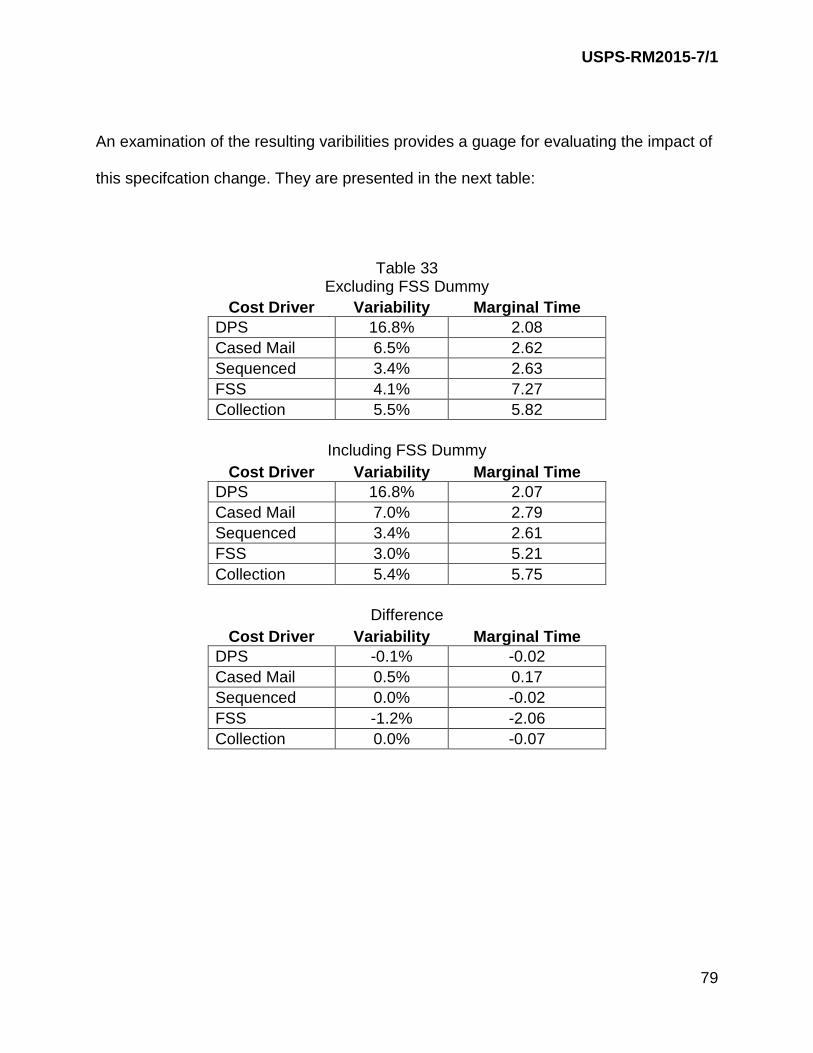
USPS-RM2015-7/1

79

An examination of the resulting varibilities provides a guage for evaluating the impact of

this specifcation change. They are presented in the next table:

Table 33 Excluding FSS Dummy

Cost Driver Variability Marginal Time DPS 16.8% 2.08 Cased Mail 6.5% 2.62 Sequenced 3.4% 2.63 FSS 4.1% 7.27 Collection 5.5% 5.82

Including FSS Dummy Cost Driver Variability Marginal Time

DPS 16.8% 2.07 Cased Mail 7.0% 2.79 Sequenced 3.4% 2.61 FSS 3.0% 5.21 Collection 5.4% 5.75

Difference Cost Driver Variability Marginal Time

DPS -0.1% -0.02 Cased Mail 0.5% 0.17 Sequenced 0.0% -0.02 FSS -1.2% -2.06 Collection 0.0% -0.07

USPS-RM2015-7/1

80

The variabillites and marginal times for DPS volume, sequenced volume, and

collection volume are not affected. The variability and marginal time for cased mail are

slightly increased. The variability for FSS mail falls by over one percent and the

marginal time falls by two seconds. This change puts the FSS marginal time more in

line with the other estimated marginal times from the model.

A final issue to be investigated is the possibility of a small number of atypical

observations having an undue impact on the estimated regression equation. To identify

potentially troublesome observations, one must identify those observations which are

both far from the regression line and have the potential to influence the estimated

coefficients.27 To investigate this possibility, the individual observations are examined

to see which are both far from the regression line and potentially influential.

“Studentized Residuals" can be used to identify outliers. The Studentized

Residual measures the distance to the observation from the regression line. To

calculate the measure, one divides the value for the ith residual by the standard error of

the residuals with the ith residual removed:28

𝑒𝑒𝑟𝑟𝑖𝑖 = 𝑒𝑒𝑖𝑖

𝜎𝜎�(𝑒𝑒𝑖𝑖).

This statistic gives a scaled, and thus comparable, measure of distance for each

observation from the regression line. In large samples, the cutoff value for potential

27 For a detailed discussion of outliers and their potential effect on the regression equation, see “Report on Updating the Cost-to-Capacity Variabilities for Purchased Highway Transportation,’ USPS-RM2014-6/1, Docket No. RM2004-1. 28 The residual in a regression equation is equal to the difference between the actual value for the dependent variable for a given observation and its predicted value.

USPS-RM2015-7/1

81

outliers is typically 2.5, but based upon the t-distribution, a more conservative cutoff

value is 2.0 which is applied here.

“Leverage” can be used to identify potentially influential observations as it

measures how "far" a given observation on the right-hand-side variables is from the

centroid of the right-hand-side variables. The leverage for a given observation is:

ℎ𝑖𝑖 = 1𝑛𝑛 + 𝑥𝑥𝑖𝑖(𝑋𝑋′𝑋𝑋)−1𝑥𝑥𝑖𝑖.′

Note that xi is the row of the matrix of right-hand-side variables (X) that contains

the ith observation. The cutoff for observations with high leverage is given by 2*(p/n),

where "p" is the number of right-hand-side variables and "n" is the number of

observations. For the regular delivery equation the cut off value is 2 *(27/3485) =

0.0155.

There are 44 observations that are both outliers and have high leverage. This is

the set of potentially influential observations that could unduly affect the estimated

coefficients used to calculate the delivery time variabilities. A complete list of the

observations is provided in USPS-RM2015-7/1, but important characteristics of these

observations are discussed below.29

First, note that there is a tendency for these of observations to occur more than

once in a ZIP Code. The 44 observations are clustered in just 18 ZIP Codes. ZIP

29 This discussion is responsive to the Commission’s order that the “Postal Service should describe the nature of excluded observations when it uses this method as it did in the case of excluded inter-Cluster tractor trailer observations.” See, Postal Regulatory Commission, “Order No. 2180 on Analytical Principles Used In Periodic Reporting,” Docket No. RM 2014-6 (Sept. 10, 2014) at 15.

USPS-RM2015-7/1

82

Code 10456, in the Bronx, has six of these outlier observations; ZIP Code 60634, in

Chicago has seven of these outlier observations; and ZIP Code 77573, outside

Houston, has five of these outlier observations.

Table 35

Sources of Potentially Influential Observations

Masked Zip Code # of Potential Influential Obs.

68555 1 83226 2 26979 1 49047 2 42765 4 55433 6 15092 1 97116 1 68245 1 31736 7 44113 4 57737 1 48719 5 76688 2 84931 2 49771 1 59701 1 83077 2

Second, note that nearly half of the observations occur on Mondays, suggesting

that the potentially influential observations may be associated with high volume days.

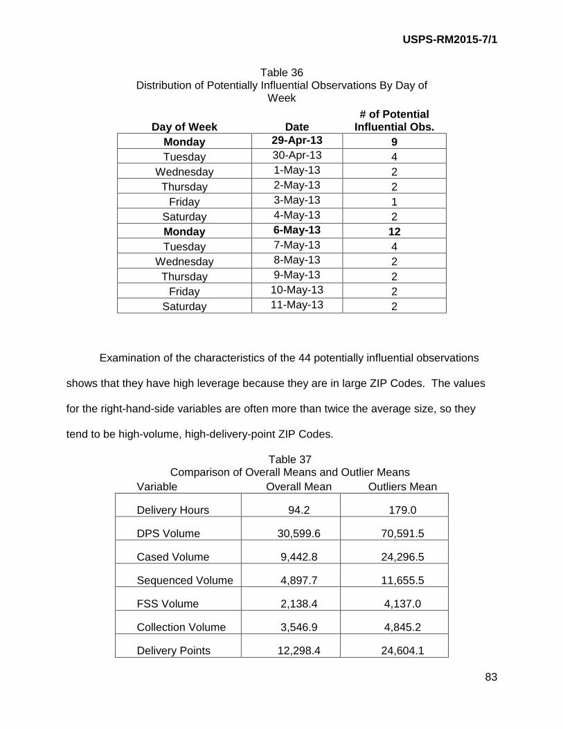
USPS-RM2015-7/1

83

Table 36 Distribution of Potentially Influential Observations By Day of

Week

Day of Week Date # of Potential

Influential Obs. Monday 29-Apr-13 9 Tuesday 30-Apr-13 4

Wednesday 1-May-13 2 Thursday 2-May-13 2

Friday 3-May-13 1 Saturday 4-May-13 2 Monday 6-May-13 12 Tuesday 7-May-13 4

Wednesday 8-May-13 2 Thursday 9-May-13 2

Friday 10-May-13 2 Saturday 11-May-13 2

Examination of the characteristics of the 44 potentially influential observations

shows that they have high leverage because they are in large ZIP Codes. The values

for the right-hand-side variables are often more than twice the average size, so they

tend to be high-volume, high-delivery-point ZIP Codes.

Table 37 Comparison of Overall Means and Outlier Means

Variable Overall Mean Outliers Mean

Delivery Hours 94.2 179.0

DPS Volume 30,599.6 70,591.5

Cased Volume 9,442.8 24,296.5

Sequenced Volume 4,897.7 11,655.5

FSS Volume 2,138.4 4,137.0

Collection Volume 3,546.9 4,845.2

Delivery Points 12,298.4 24,604.1

USPS-RM2015-7/1

84

The ultimate test of potential influence is given by re-estimating the equation with

the outlier(s) omitted and comparing the resulting coefficients with the original

coefficients. To do this, the regular delivery time equation was re-estimated after

dropping the 44 potentially influential observations. The complete results are given in

USPS-RM2015-7/1, but in summary, dropping the observations had surprisingly little

impact on the estimation. All of the coefficients remain statistically significant and none

switch signs. More importantly, as the following table shows, eliminating these 44

outliers does not materially affect the estimated variabilities.

Table 38 Delivery Time Variabilities from the Regular Delivery Equation

Review of the data for the 44 observations reveals nothing to suggest that the

observations contain data errors or do not come from valid ZIP Codes that perform

standard city carrier delivery operations. Rather they are made up of high volume days

in large ZIP Codes. Given that these observations do not seem particularly unusual and

All Observations

Dropping 44 Outliers Difference

DPS Volume 0.1676 0.1594 -0.0083

Cased Volume 0.0699 0.0763 0.0064

Sequenced Volume 0.0338 0.0344 0.0006

FSS Volume 0.0295 0.0303 0.0008

Collection Volume 0.0541 0.0569 0.0029

Delivery Points 0.5491 0.5522 0.0030

USPS-RM2015-7/1

85

that they do not exhibit undue influence on the estimated coefficients, it is preferred to

leave them in the data set when estimating the regression.

IV. ESTIMATING THE PACKAGE AND ACCOUNTABLE DELIVERY EQUATIONS AND CALCULATING THE ASSOCIATED VARIABILITIES

A. Introduction

Regular delivery time covers the delivery of letters and flats throughout the Postal

Service’s network of city carrier letter routes. It does not include the time required for

delivering packages and accountables.30 Moreover, finding the street time costs for

packages and accountable can be a challenge, for several reasons.

First, the volume of packages delivered is very small relative to the volumes of

letters and flats delivered. A typical city route, on an average day, delivers about 2,300

letters and flats to about 600 delivery points. But that same typical route will deliver only

30 to 40 packages. This means that fewer than 5 percent of delivery points get a

package on a typical day, and that packages represent under 2 percent of total

delivered volume. Consequently, the delivery time for packages is an order of

magnitude smaller than the delivery time for letters and flats, and the impact of package

delivery on total delivery time can be overwhelmed by the impact of letter and flat

delivery. This makes it extremely difficult to estimate a package variability jointly with

letter and flat variabilities.

30 The one exception is for small packages (according to their DMM definition) that are handled like flats in the office and cased along with residual letters and flat. From the perspective of street time costs, these pieces are handled just like the other pieces of cased mail and thus are included in the cased mail bundle in the regular delivery equation.

USPS-RM2015-7/1

86

The volume of accountables is even smaller than the volume of packages, with a

typical route delivering just a handful per day. Despite the fact that accountable delivery

is time consuming, on a per-piece basis, it accounts for a tiny amount of total street

time. Finally, packages are handled in different ways in delivery, depending upon their

size, and this complicates the task of measuring a street time variability for packages.

For these reasons, it is logical to pursue a separate analysis to measure the attributable

costs of packages and accountables.

Investigation of Postal Service data systems revealed that its carrier databases

do not include complete data on package and accountable delivery times and volumes.

Therefore, a special field study was required to collect the data needed for estimating

package and accountable attributable costs.

Estimating package and accountable variabilities takes the same general steps as

estimating the variabilities for letters and flats. It requires specifying models of package

and accountable delivery, collecting the data, constructing the relevant analysis data

set, econometrically estimating the specified models with the analysis data set and then

reviewing and evaluating the results. Each of these steps is described, in turn, in this

section.

B. Specifying the Package and Accountable Models to be Estimated

There are three separate delivery activities included in total package and

accountable delivery time: the delivery of packages which fit into the mail receptacle,

the delivery of packages that require a carrier deviation or change in the regular delivery

procedures, and the delivery of accountables which require a signature or customer

USPS-RM2015-7/1

87

contact.31 As with regular delivery, the cost drivers of package and accountable

delivery are the volumes delivered and the number of delivery points to be covered.

Package and accountable delivery is also affected by the environment in which

delivery takes place, but the relevant characteristic variables are somewhat different

from those describing the letter and flat delivery environment. For regular delivery, the

three characteristic variables are: (1) the primary delivery technology used in the ZIP

Code, (2) the proportion of business deliveries in the ZIP Code, and the (3)

geographical density of delivery points in the ZIP Code. Each of these can be reviewed

for its applicability to package and accountable delivery.

While package and accountable delivery is affected by the delivery technology, it

is not affected by the overall delivery technology of the route, but rather the delivery

technology of package and accountable deliveries made. Because there are so few

package and accountable deliveries made on a route, it could well be that the route’s

overall delivery type does not reflect the delivery technology for its package and

accountable delivery.

For example, it could be that on a given day, all of a route’s packages are

delivered to a cluster box, even though the route is predominantly park and loop. To

accurately capture the nature of package and accountable delivery, the package

delivery time equations will include the proportions of the package and accountable

deliveries made by mode. In other words, to control for different delivery environments,

31 Packages that are also accountables are treated as accountables.

USPS-RM2015-7/1

88

the package delivery time equations will include the proportions of door, curb, cluster

box, dismount, and central package and accountable deliveries.

Because regular delivery time includes much of the time that carriers spend

traversing their routes, a measure of geographic density was included in the regular

delivery equation to control for variations in time associated with different geographic

distances. But package and accountable delivery time occurs when the carrier is at the

stop and does not depend upon the distance between stops. Accordingly, the package

and accountable equations will not include a measure of miles per delivery point. On

the other hand, package and accountable delivery time, like regular delivery time, could

be affected by the presence of business deliveries, so the package and accountable

equations will include the proportion of business delivery points.

In-receptacle packages are delivered in the same receptacle as letters and flats,

and are delivered in the course of the carrier’s regular line of travel, using regular

delivery procedures. The actions required to deliver in-receptacle packages are not,

consequently, related to the actions required to deliver deviation packages and

accountables. It is appropriate, therefore, to specify a separate equation for in-

receptacle package delivery. A ZIP Code’s volume of in-receptacle packages and its

delivery points are the cost drivers for an in-receptacle package delivery time equation.

The characteristic variables included to control for variations in the delivery environment

are the proportions of in-receptacle deliveries, by mode, and the proportion of business

deliveries.32

32 The five different mode of delivery proportions sum to one and thus, along with the intercept, they form a linear combination. Consequently, only four of the five proportions can be included in the equation.

USPS-RM2015-7/1

89

The in-receptacle package delivery time equation has a quadratic form:

𝑉𝑉𝐵𝐵𝐷𝐷𝐷𝐷𝐷𝐷𝑖𝑖𝑖𝑖 = 𝜆𝜆0 + 𝜆𝜆1𝑉𝑉𝐵𝐵𝐷𝐷𝑖𝑖𝑖𝑖 + 𝜆𝜆11𝑉𝑉𝐵𝐵𝐷𝐷𝑖𝑖𝑖𝑖2 + 𝜆𝜆2 𝐷𝐷𝐷𝐷𝑖𝑖𝑖𝑖 + 𝜆𝜆22𝐷𝐷𝐷𝐷𝑖𝑖𝑖𝑖2 + 𝜆𝜆12 𝑉𝑉𝐵𝐵𝐷𝐷𝑖𝑖𝑖𝑖 ∗ 𝐷𝐷𝐷𝐷𝑖𝑖𝑖𝑖 + 𝜆𝜆3 𝜌𝜌𝐷𝐷𝐵𝐵𝑖𝑖𝑖𝑖

+ 𝜆𝜆4 𝜌𝜌𝐶𝐶𝐵𝐵𝑖𝑖𝑖𝑖 + 𝜆𝜆5𝜌𝜌𝐷𝐷𝐶𝐶𝑖𝑖𝑖𝑖 + 𝜆𝜆6 𝜌𝜌𝐶𝐶𝑆𝑆𝑁𝑁𝑖𝑖𝑖𝑖 + 𝜆𝜆7 𝐵𝐵𝐵𝐵𝑖𝑖𝑖𝑖 + 𝜈𝜈𝑖𝑖𝑖𝑖

Where:

IRPDT = In-Receptacle Package Delivery Time IRP = In-Receptacle Package Volume DP = Delivery Points ρDR = Proportion of Door In-Receptacle Deliveries ρCR = Proportion of Curb In-Receptacle Deliveries ρDM = Proportion of Dismount In-Receptacle Deliveries ρCEN = Proportion of Central In-Receptacle Deliveries BR = Proportion of Business Deliveries

Both deviation package and accountable deliveries require the carrier to deviate

from the regular delivery procedures and either make customer contact or make the

delivery in a place other than the customer’s regular receptacle. This means that

deviation packages and accountables can be and are delivered together. In addition,

on driving routes, a deviation delivery for a deviation package, an accountable, or both,

may require a “move vehicle” delivery. When there are both deviation packages and

accountables being delivered in this type of delivery, the move vehicle time is jointly

caused by the two products. For these reasons, it is appropriate to estimate a joint

equation for deviation packages and accountables.33 The dependent variable will be

deviation delivery time, which is the sum of deviation package delivery time,

33 This specification was proposed by the Postal Service and accepted by the Commission in Docket No. R2005-1.

USPS-RM2015-7/1

90

accountable delivery time, and move vehicle time. The deviation delivery equation also

has a quadratic specification.

𝐷𝐷𝑆𝑆𝐶𝐶𝐷𝐷𝐷𝐷𝑖𝑖𝑖𝑖 = 𝜓𝜓0 + 𝜓𝜓1𝐷𝐷𝑆𝑆𝐶𝐶𝐷𝐷𝑖𝑖𝑖𝑖 + 𝜓𝜓11𝐷𝐷𝑆𝑆𝐶𝐶𝐷𝐷𝑖𝑖𝑖𝑖2 + 𝜓𝜓2 𝐴𝐴𝐶𝐶𝐷𝐷𝑖𝑖𝑖𝑖 + 𝜓𝜓22𝐴𝐴𝐶𝐶𝐷𝐷𝑖𝑖𝑖𝑖2 + 𝜓𝜓3 𝐷𝐷𝐷𝐷𝑖𝑖𝑖𝑖 + 𝜓𝜓33𝐷𝐷𝐷𝐷𝑖𝑖𝑖𝑖2

+ 𝜓𝜓12 𝐷𝐷𝑆𝑆𝐶𝐶𝐷𝐷𝑖𝑖𝑖𝑖 ∗ 𝐴𝐴𝐶𝐶𝐷𝐷𝑖𝑖𝑖𝑖 + 𝜓𝜓12 𝐷𝐷𝑆𝑆𝐶𝐶𝑖𝑖𝑖𝑖 ∗ 𝐷𝐷𝐷𝐷𝑖𝑖𝑖𝑖 + 𝜓𝜓23 𝐴𝐴𝐶𝐶𝐷𝐷𝑖𝑖𝑖𝑖 ∗ 𝐷𝐷𝐷𝐷𝑖𝑖𝑖𝑖 + 𝜓𝜓4 𝜌𝜌𝐶𝐶𝐵𝐵𝜌𝜌𝑖𝑖𝑖𝑖

+ 𝜓𝜓5 𝜌𝜌𝐶𝐶𝐵𝐵𝑖𝑖𝑖𝑖 + 𝜓𝜓6 𝜌𝜌𝐷𝐷𝐶𝐶𝑖𝑖𝑖𝑖 + 𝜓𝜓7 𝜌𝜌𝐶𝐶𝑆𝑆𝑁𝑁𝑖𝑖𝑖𝑖 + 𝜓𝜓8 𝐵𝐵𝐵𝐵𝑖𝑖𝑖𝑖 + 𝜉𝜉𝑖𝑖𝑖𝑖

Where:

DEVDT = Deviation Delivery Time DEVP = Deviation Package Volume ACT = Accountable Volume DP = Delivery Points ρCBU = Proportion of Cluster Box In-Receptacle Deliveries ρCR = Proportion of Curb In-Receptacle Deliveries ρDM = Proportion of Dismount In-Receptacle Deliveries ρCEN = Proportion of Central In-Receptacle Deliveries BR = Proportion of Business Deliveries

The data required to estimate these equations is not currently collected within the

Postal Service’s carrier data systems, so a field study was required to collect the

requisite data. That study is described in the next subsection.

USPS-RM2015-7/1

91

C. The Package and Accountable Field Study

The package and accountable field study was designed to record both volumes

and delivery times for five package/accountable activities:

• Delivery of in-receptacle packages. • Delivery of deviation packages. • Delivery of accountables. • Deliveries of packages or accountables that require an extra vehicle movement. • Collection of prescheduled Package Pickups.

The sample for the field study was the same 300 ZIP Codes that were included in the

collection volume study, and were thus used to estimate the regular delivery equation.

The package and accountable field study was carried out with the following steps:

1. The study process was designed.

2. A beta test of the study was performed and the study process was refined.

3. The full data collection effort was launched.

4. The collected data were analyzed.

Each of these steps is discussed in the following subsections.

1. Designing the study process

Delivery times for the various activities were developed by having carriers self-

record the time they spent in each activity. The times were recorded by carriers using

their hand-held scanners, which they now use on a daily basis, to scan a limited number

of special barcodes, indicating that a particular activity was starting or finishing. The

elapsed time for the activity was measured as the difference between the initial scan

(indicating the activity was starting) and the terminal scan (indicating the activity was

USPS-RM2015-7/1

92

finished). Volumes were counted and collected through a webtool similar to the one

used in the collection volume study.

2. Performing a beta test

A beta test of the package and accountable field study was performed at seven

ZIP Codes over the six delivery day period from January 27 through February 1, 2014.

The beta test provided an opportunity to see if the instructions and training were

sufficient to allow the carriers to accurately record their package and accountable

delivery times and to accurately count and record their package and accountable

volumes.

The beta test successfully provided a proof of concept that carriers were able to

understand the study process and complete the required scans. It also showed that the

carriers were able to successfully record their delivered volumes of in-receptacle

packages, deviation packages, and accountables. In addition, an important refinement

resulted from the beta test. The beta test caused the study team to recognize that the

scan sequence could be simplified from a three-scan process: scan Begin Delivery

barcode → scan End Delivery barcode → scan Mode barcode, to just a two-scan

process: scan Begin Delivery barcode → scan Mode barcode. The simplified scanning

system provided the same information as the three-scan process and allowed all activity

time to be recorded with just ten different bar codes, reducing the complexity of the

process and reducing the potential for errors while providing the necessary information

about delivery mode and the end delivery time simultaneously.

For example, suppose bar code 310 was for recording the beginning of an in-

receptacle package delivery. Under the two-scan method, a carrier would use the hand

USPS-RM2015-7/1

93

held scanner to scan barcode 310 when he or she was just beginning an in-receptacle

package delivery. When the delivery was finished, the carrier would then scan one of

five mode scans, depending upon the type of delivery. As well as recording the mode of

delivery, scanning the mode barcode indicated when the in-receptacle delivery was

over. The elapsed time for that delivery would be the difference between the recorded

time for the in-receptacle package scan and the recorded time for the mode scan. The

two barcode process is highlighted in the following figure.

Figure 11: Barcode Pairs for In-Receptacle Package Delivery

3. Launching the data collection effort Prior to launching the study, extensive training was provided, including the use of

both video materials and written training documents. Following training, the main study

was carried out for a two-week period from March 25 through April 7, 2014. Of the 300

ZIP Codes in the original sample, 289 were able to participate in the package and

accountable study.

310

365 372 389 396 402

In-Receptacle Package

Door Curb CBU Dismount Central

USPS-RM2015-7/1

94

Not all ZIP Codes were able to provide both scan and volume data for all twelve

days of the study, and a few ZIP Codes were able to provide only a few days of data.

To ensure reliability, a ZIP Code’s data were included in the study data set only if the

ZIP Code was able to provide at least one full week’s worth of data. This leads to a

total of 282 ZIP Codes being included in the study’s data set. As Table 39 shows, most

of the included ZIP Codes were able to provide both scan and volume data for all twelve

days the study.

Table 39

Pattern of ZIP Codes' Reporting Days # of Days Reporting Both Volume & Scan

Data ZIP Codes With That

Number of Reported Days 6 2

7 0

8 2

9 5

10 5

11 9

12 259

While a few ZIP Codes were late starting their participation in the study, the

primary reason that a ZIP Code did not provide all twelve days of data is that it stopped

participating before the end of the study. There are a total of 54 ZIP Code days missing

from a possible total of 3,384 ZIP Code days (12 days times 292 ZIP Codes). This is a

loss of 1.6 percent of the possible ZIP Code days. The next figure visually shows the

pattern of ZIP Code day attrition. As expected, there are more ZIP Code days lost at

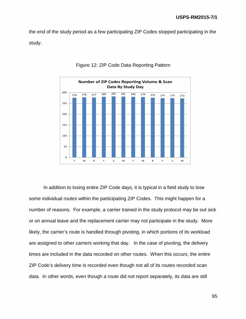
USPS-RM2015-7/1

95

the end of the study period as a few participating ZIP Codes stopped participating in the

study.

Figure 12: ZIP Code Data Reporting Pattern

In addition to losing entire ZIP Code days, it is typical in a field study to lose

some individual routes within the participating ZIP Codes. This might happen for a

number of reasons. For example, a carrier trained in the study protocol may be out sick

or on annual leave and the replacement carrier may not participate in the study. More

likely, the carrier’s route is handled through pivoting, in which portions of its workload

are assigned to other carriers working that day. In the case of pivoting, the delivery

times are included in the data recorded on other routes. When this occurs, the entire

ZIP Code’s delivery time is recorded even though not all of its routes recorded scan

data. In other words, even though a route did not report separately, its data are still

276 278 277 280 282 281 280 279 276 274 274 273

0

50

100

150

200

250

300

T W R F S M T W R F S M

Number of ZIP Codes Reporting Volume & Scan Data By Study Day

USPS-RM2015-7/1

96

included in the overall ZIP Code values. Finally, it is possible that a carrier may have

suffered from “study fatigue,” meaning they simply stopped participating before the end

of the study period.

While all three reasons likely occurred during the package and accountable

study, there is some evidence, as shown in the next figure, of modest study fatigue. The

number of routes reporting scan data fell in the second week of the study, particularly

the last few days.

Figure 13: Routes Reporting Scan Data by Date

This pattern of attrition was anticipated when the study was designed and was

part of the motivation for selecting a two-week period rather than a one-week period. In

addition, possible attrition was part of the reason that a large number of ZIP Codes were

included in the sample. Most importantly, subsequent analysis showed that neither ZIP

0

1000

2000

3000

4000

5000

6000

Number of Routes Reporting Scan Data by Study Date

USPS-RM2015-7/1

97

Code nor route attrition materially affected the estimated variabilities. Experiments of

re-estimating the models with just the first week of data or with dropping just the last

couple of days of data produced variabilities quite close to those estimated on the full

data set.34

The next table provides some basic route-day statistics from the sample. During

the study period, there were, on average, 41 packages delivered per route per day.

About 60 percent of those packages were delivered in-receptacle. The average number

of accountables delivered per route per day was just 2.8. In addition, neither

prescheduled package pickups nor on-demand pickups were large enough to merit

further investigation. The median pickup volume for all categories was zero and

approximately 90 percent of routes had no package pickup or on-demand volumes over

the two-week period.

34 For example, the in-receptacle package variability, estimated on the full data set was 48.8 percent. Re-estimating the in-receptacle package equation dropping the last day, the last two days, the last three days and the last four days of data yielded variabilities of 49.2 percent, 49.4 percent and 49.5 and 49.1 percent, respectively. Estimating the model on just the first week of data yielded a variability of 47.5 percent.

USPS-RM2015-7/1

98

4. Analyzing the collected data

There were two data issues that needed to be addressed before the analysis

data set could be constructed. First, the sequence of actions used to record the

barcodes during the study caused the recorded delivery times to be inflated by the time

it took for scanning the mode barcode. Recall that the scanning sequence for each

activity started with a begin activity scan and ended with the mode scan. For example,

an in-receptacle package delivery at a cluster box would start with the carrier scanning

the “Begin In-Receptacle Package Delivery” barcode and would end with the carrier

scanning the “NDCBU Delivery” barcode. The activity time was then computed as the

elapsed time between the time stamp for the begin activity scan and the time stamp for

the mode scan.

Average MedianInter Quartile

Range Minimum Maximum

IN RECEPTACLE PACKAGES 24.5 23.0 13-33 0 1,000

DEVIATION PACKAGES 16.6 15.0 8-22 0 718

ACCOUNTABLES 2.8 2.0 0-4 0 432

PP EXPRESS COLLECTED 0.3 0.0 0-0 0 127

PP PRIORITY COLLECTED 0.0 0.0 0-0 0 80

PP FIRST CLASS COLLECTED 0.9 0.0 0-0 0 1,393

PP OTHER COLLECTED 1.2 0.0 0-0 0 1,811

OD EXPRESS COLLECTED 0.2 0.0 0-0 0 220

OD PRIORITY COLLECTED 0.0 0.0 0-0 0 116

OD FIRST CLASS COLLECTED 0.0 0.0 0-0 0 151

OD OTHER COLLECTED 0.0 0.0 0-0 0 87

Average Daily Volumes Per RouteTable 40

USPS-RM2015-7/1

99

The study instructions required the carrier to scan the “Begin In-Receptacle

Package Delivery” barcode before beginning the in-receptacle package delivery, so the

time to scan that barcode was not included in the elapsed time. But, by the nature of

the process, the “NDCBU Delivery” barcode could not be scanned until after the in-

receptacle package delivery was completed. This means that the recorded elapsed

time included both the time it took to deliver the package and the time it took to scan the

mode barcode.

To account for this extra time, participating ZIP Codes were asked to keep track

of the additional daily street time that was required to complete the study scans.

Dividing this additional time by the number of barcode scans taken produced the

average time per study scan of 12 seconds. Consequently, to adjust for the inclusion of

study scanning time, the elapsed time for each activity pair was reduced by 12 seconds.

The second data issue to be examined also related to the scanning process. To

fully record each barcode, a carrier was required to perform three actions: read the

barcode with the scanner, press the “enter” key to record the activity, and then press the

“A” key to record the time stamp. Thus, to accurately record the elapsed time for an

activity, the carrier needed to undertake six physical actions: To record the time when

the activity started required scanning the barcode, then hitting the “Enter” key and then

hitting the ”A” key. To record the time when the activity finished required scanning the

barcode, then hitting the “Enter” key and then hitting the ”A” key.

If the carrier failed to hit the “A” key for the begin activity scan, then the time

stamp was not recorded for the beginning of the activity and both the begin activity scan

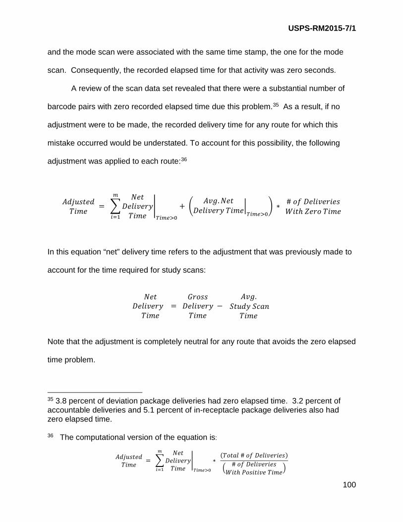
USPS-RM2015-7/1

100

and the mode scan were associated with the same time stamp, the one for the mode

scan. Consequently, the recorded elapsed time for that activity was zero seconds.

A review of the scan data set revealed that there were a substantial number of

barcode pairs with zero recorded elapsed time due this problem.35 As a result, if no

adjustment were to be made, the recorded delivery time for any route for which this

mistake occurred would be understated. To account for this possibility, the following

adjustment was applied to each route:36

𝐴𝐴𝐶𝐶𝐴𝐴𝑢𝑢𝐴𝐴𝐶𝐶𝑒𝑒𝐶𝐶𝐷𝐷𝐶𝐶𝑇𝑇𝑒𝑒 = �

𝑁𝑁𝑒𝑒𝐶𝐶𝐷𝐷𝑒𝑒𝐷𝐷𝐶𝐶𝐷𝐷𝑒𝑒𝐷𝐷𝑦𝑦𝐷𝐷𝐶𝐶𝑇𝑇𝑒𝑒

�𝑇𝑇𝑖𝑖𝑚𝑚𝑇𝑇>0

𝑚𝑚

𝑖𝑖=1

+ �𝐴𝐴𝐷𝐷𝐴𝐴.𝑁𝑁𝑒𝑒𝐶𝐶

𝐷𝐷𝑒𝑒𝐷𝐷𝐶𝐶𝐷𝐷𝑒𝑒𝐷𝐷𝑦𝑦 𝐷𝐷𝐶𝐶𝑇𝑇𝑒𝑒�𝑇𝑇𝑖𝑖𝑚𝑚𝑇𝑇>0� ∗ # 𝐶𝐶𝑖𝑖 𝐷𝐷𝑒𝑒𝐷𝐷𝐶𝐶𝐷𝐷𝑒𝑒𝐷𝐷𝐶𝐶𝑒𝑒𝐴𝐴

𝑊𝑊𝐶𝐶𝐶𝐶ℎ 𝑍𝑍𝑒𝑒𝐷𝐷𝐶𝐶 𝐷𝐷𝐶𝐶𝑇𝑇𝑒𝑒

In this equation “net” delivery time refers to the adjustment that was previously made to

account for the time required for study scans:

𝑁𝑁𝑒𝑒𝐶𝐶

𝐷𝐷𝑒𝑒𝐷𝐷𝐶𝐶𝐷𝐷𝑒𝑒𝐷𝐷𝑦𝑦 𝐷𝐷𝐶𝐶𝑇𝑇𝑒𝑒

= 𝐺𝐺𝐷𝐷𝐶𝐶𝐴𝐴𝐴𝐴

𝐷𝐷𝑒𝑒𝐷𝐷𝐶𝐶𝐷𝐷𝑒𝑒𝐷𝐷𝑦𝑦𝐷𝐷𝐶𝐶𝑇𝑇𝑒𝑒

− 𝐴𝐴𝐷𝐷𝐴𝐴.

𝐷𝐷𝐶𝐶𝑢𝑢𝐶𝐶𝑦𝑦 𝐷𝐷𝑆𝑆𝑆𝑆𝑛𝑛 𝐷𝐷𝐶𝐶𝑇𝑇𝑒𝑒

Note that the adjustment is completely neutral for any route that avoids the zero elapsed

time problem.

35 3.8 percent of deviation package deliveries had zero elapsed time. 3.2 percent of accountable deliveries and 5.1 percent of in-receptacle package deliveries also had zero elapsed time. 36 The computational version of the equation is:

𝐴𝐴𝐶𝐶𝐴𝐴𝑢𝑢𝐴𝐴𝐶𝐶𝑒𝑒𝐶𝐶𝐷𝐷𝐶𝐶𝑇𝑇𝑒𝑒 = �

𝑁𝑁𝑒𝑒𝐶𝐶𝐷𝐷𝑒𝑒𝐷𝐷𝐶𝐶𝐷𝐷𝑒𝑒𝐷𝐷𝑦𝑦𝐷𝐷𝐶𝐶𝑇𝑇𝑒𝑒

�𝑇𝑇𝑖𝑖𝑚𝑚𝑇𝑇>0

𝑚𝑚

𝑖𝑖=1

∗ (𝐷𝐷𝐶𝐶𝐶𝐶𝑆𝑆𝐷𝐷 # 𝐶𝐶𝑖𝑖 𝐷𝐷𝑒𝑒𝐷𝐷𝐶𝐶𝐷𝐷𝑒𝑒𝐷𝐷𝐶𝐶𝑒𝑒𝐴𝐴)

� # 𝐶𝐶𝑖𝑖 𝐷𝐷𝑒𝑒𝐷𝐷𝐶𝐶𝐷𝐷𝑒𝑒𝐷𝐷𝐶𝐶𝑒𝑒𝐴𝐴𝑊𝑊𝐶𝐶𝐶𝐶ℎ 𝐷𝐷𝐶𝐶𝐴𝐴𝐶𝐶𝐶𝐶𝐶𝐶𝐷𝐷𝑒𝑒 𝐷𝐷𝐶𝐶𝑇𝑇𝑒𝑒

�

USPS-RM2015-7/1

101

D. Constructing the Analysis Dataset

The analysis data set was constructed by merging the scan data set with the

volume data set. There were 3,332 ZIP Code days in the volume data set and 3,369

ZIP Code days in the scan data set. Matching the two data sets constructed an analysis

data set with 3,330 ZIP Code days. There were 2 ZIP Code days in the volume data set

for which there were no matching scan data and 39 ZIP Code days in the scan data set

for which there were no matching volume data. The analysis data set thus contains

3,330 of the possible 3,384 ZIP Code days or 98.4 percent of possible observations.

The package and accountable scan data were self-reported by carriers and thus

were potentially subject to data reporting errors. This possibility was investigated after

the scan and volume data were combined by looking at ZIP Codes with unreasonably

high or low productivities as measured by delivered time per piece. Discussion with

operations experts lead to the establishment of possible high and low productivity

cutoffs, beyond which the ZIP Code data may reflect infeasible operations.

Table 41

Potential High and Low Productivity Filters

Shape High End Value Low End Value In Receptacle Package 3 minutes 10 seconds

Deviation Package 5 minutes 10 seconds

Accountable 10 minutes 20 seconds

Application of the high-end cutoff is relatively straightforward, but economies of

density in delivery makes it more difficult to establish a low-end cutoff. It is important to

USPS-RM2015-7/1

102

exclude only truly infeasible data, and if a ZIP Code had very high in-receptacle

volumes, it may be possible for it to average very low average delivery times per piece

because of economies of density. If so, the ZIP Code data are valid and should be

included. The goal is to develop an algorithm to identify just those ZIP Code days with

infeasible data. For example, if a ZIP Code experienced a shortage of routes reporting

scan time on a given day but complete reporting of volume, then it will have apparently

low delivery times per piece. But, the observed low delivery times per piece were

artificial, and that ZIP Code day’s data should be dropped from the analysis data set.

To accommodate these different reasons for low average delivery times per

piece, the low-end cutoff was modified in two ways. First, if a ZIP Code day averaged

more than two pieces per delivery point for in-receptacle delivery, then its data were

preserved, even if it had very low average times per piece. This captures the impact of

economies of density on average delivery times. In contrast, to identify artificially low

average delivery times, an indicator of under reporting, called the “route gap”, was

constructed. The route gap was designed to identify the percentage of routes within a

ZIP Code not reporting scan data on a given day.37 The route gap indictor is given by:

𝐵𝐵𝐶𝐶𝑢𝑢𝐶𝐶𝑒𝑒 𝐺𝐺𝑆𝑆𝐺𝐺 = (#𝐶𝐶𝑖𝑖 𝐵𝐵𝑒𝑒𝐺𝐺𝐶𝐶𝐷𝐷𝐶𝐶𝐶𝐶𝑛𝑛𝐴𝐴 𝐶𝐶𝐶𝐶𝐷𝐷𝑢𝑢𝑇𝑇𝑒𝑒 𝐵𝐵𝐶𝐶𝑢𝑢𝐶𝐶𝑒𝑒𝐴𝐴 − #𝐶𝐶𝑖𝑖 𝐵𝐵𝑒𝑒𝐺𝐺𝐶𝐶𝐷𝐷𝐶𝐶𝐶𝐶𝑛𝑛𝐴𝐴 𝐷𝐷𝑆𝑆𝑆𝑆𝑛𝑛 𝐵𝐵𝐶𝐶𝑢𝑢𝐶𝐶𝑒𝑒𝐴𝐴)

#𝐶𝐶𝑖𝑖 𝐵𝐵𝑒𝑒𝐺𝐺𝐶𝐶𝐷𝐷𝐶𝐶𝐶𝐶𝑛𝑛𝐴𝐴 𝐶𝐶𝐶𝐶𝐷𝐷𝑢𝑢𝑇𝑇𝑒𝑒 𝐵𝐵𝐶𝐶𝑢𝑢𝐶𝐶𝑒𝑒𝐴𝐴

37 Because of pivoting, it is quite possible that a ZIP Code could accurately have fewer routes reporting scan data than volume data. The volume would be counted in the office and assigned to a pivoted route, but the scan would be recorded on the routes that picked up the portions of the pivoted route.

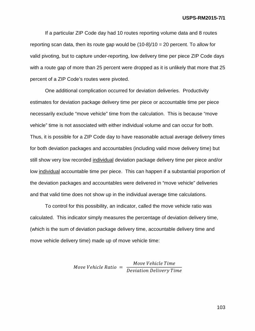
USPS-RM2015-7/1

103

If a particular ZIP Code day had 10 routes reporting volume data and 8 routes

reporting scan data, then its route gap would be (10-8)/10 = 20 percent. To allow for

valid pivoting, but to capture under-reporting, low delivery time per piece ZIP Code days

with a route gap of more than 25 percent were dropped as it is unlikely that more that 25

percent of a ZIP Code’s routes were pivoted.

One additional complication occurred for deviation deliveries. Productivity

estimates for deviation package delivery time per piece or accountable time per piece

necessarily exclude “move vehicle” time from the calculation. This is because “move

vehicle” time is not associated with either individual volume and can occur for both.

Thus, it is possible for a ZIP Code day to have reasonable actual average delivery times

for both deviation packages and accountables (including valid move delivery time) but

still show very low recorded individual deviation package delivery time per piece and/or

low individual accountable time per piece. This can happen if a substantial proportion of

the deviation packages and accountables were delivered in “move vehicle” deliveries

and that valid time does not show up in the individual average time calculations.

To control for this possibility, an indicator, called the move vehicle ratio was

calculated. This indicator simply measures the percentage of deviation delivery time,

(which is the sum of deviation package delivery time, accountable delivery time and

move vehicle delivery time) made up of move vehicle time:

𝐶𝐶𝐶𝐶𝐷𝐷𝑒𝑒 𝐶𝐶𝑒𝑒ℎ𝐶𝐶𝑆𝑆𝐷𝐷𝑒𝑒 𝐵𝐵𝑆𝑆𝐶𝐶𝐶𝐶𝐶𝐶 = 𝐶𝐶𝐶𝐶𝐷𝐷𝑒𝑒 𝐶𝐶𝑒𝑒ℎ𝐶𝐶𝑆𝑆𝐷𝐷𝑒𝑒 𝐷𝐷𝐶𝐶𝑇𝑇𝑒𝑒

𝐷𝐷𝑒𝑒𝐷𝐷𝐶𝐶𝑆𝑆𝐶𝐶𝐶𝐶𝐶𝐶𝑛𝑛 𝐷𝐷𝑒𝑒𝐷𝐷𝐶𝐶𝐷𝐷𝑒𝑒𝐷𝐷𝑦𝑦 𝐷𝐷𝐶𝐶𝑇𝑇𝑒𝑒

USPS-RM2015-7/1

104

If a ZIP Code day had 40 minutes of deviation package delivery time, 35 minutes

of accountable delivery time and 25 minutes of move vehicle time, then its move vehicle

ratio would be (25/(40+35+25)) or 25 percent. This indicator was used to identify high

move vehicle ZIP Codes. Thus, if a ZIP Code day had a move vehicle ratio of greater

than 25 percent, then its data were retained even if it had low deviation package or

accountable delivery times per piece.38

E. Estimating the Econometric Models and Discussion of Results

After the analysis data set was constructed, it was reviewed. That review

revealed the fact that there are some ZIP Code days with very large package and

accountable delivery time. For example, the median in-receptacle package delivery

time is 2.97 hours per ZIP Code day but there are a number of ZIP Code days with over

8 hours of in-receptacle package delivery time.

Further investigation of these large ZIP Code days suggested that their cost

generating process may be different from the rest of the ZIP Code days. This difference

is highlighted by a comparison of the cross plots between in-receptacle package time

and in-receptacle package volume for those ZIP Code days with more than 8 hours of

in-receptacle package time, and for those ZIP Code days with less than 8 hours of in-

receptacle package delivery time. These cross-plots are presented in Figure 14.

38 The median move vehicle ratio is 12.3 percent, so 25 percent is approximately twice the median value. Only 19 percent of ZIP Code days had a move vehicle ratio higher than 25 percent. Among that group, however, the average move vehicle ratio was 37.2 percent.

USPS-RM2015-7/1

105

Figure 14: Cross Plots of In-Receptacle Delivery Time and In-Receptacle Volume by Type of ZIP Code Day

These plots show a very different relationship between delivery time and volume

in the two data subsets. Because of this difference, an investigation was undertaken to

0

5000

10000

15000

20000

25000

30000

35000

0 500 1000 1500 2000 2500 3000 3500 4000

Crossplot of ZIP Code Days with Less than 8 Hours of IR Package Delivery Time

0

20000

40000

60000

80000

100000

120000

0 500 1000 1500 2000 2500 3000

Crossplot of ZIP Code Days with More than 8 Hours of IR Package Delivery Time

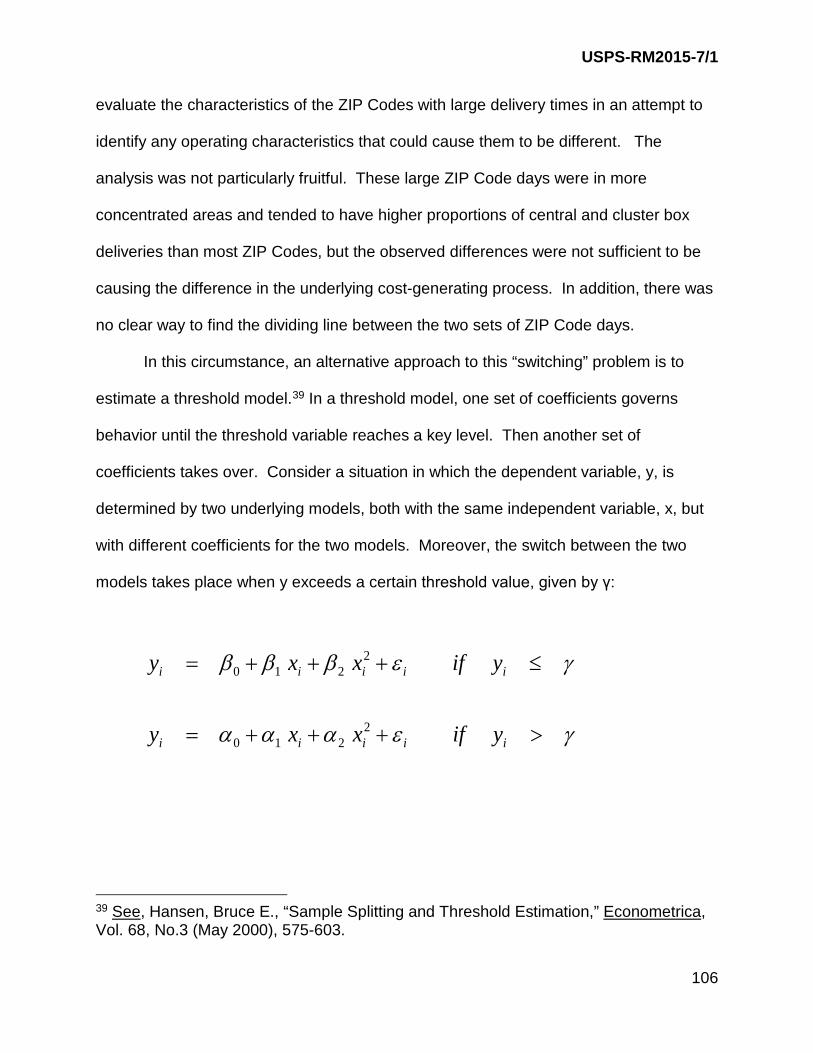
USPS-RM2015-7/1

106

evaluate the characteristics of the ZIP Codes with large delivery times in an attempt to

identify any operating characteristics that could cause them to be different. The

analysis was not particularly fruitful. These large ZIP Code days were in more

concentrated areas and tended to have higher proportions of central and cluster box

deliveries than most ZIP Codes, but the observed differences were not sufficient to be

causing the difference in the underlying cost-generating process. In addition, there was

no clear way to find the dividing line between the two sets of ZIP Code days.

In this circumstance, an alternative approach to this “switching” problem is to

estimate a threshold model.39 In a threshold model, one set of coefficients governs

behavior until the threshold variable reaches a key level. Then another set of

coefficients takes over. Consider a situation in which the dependent variable, y, is

determined by two underlying models, both with the same independent variable, x, but

with different coefficients for the two models. Moreover, the switch between the two

models takes place when y exceeds a certain threshold value, given by γ:

γεααα

γεβββ

>+++=

≤+++=

iiiii

iiiii

yifxxy

yifxxy

2210

2210

39 See, Hansen, Bruce E., “Sample Splitting and Threshold Estimation,” Econometrica, Vol. 68, No.3 (May 2000), 575-603.

USPS-RM2015-7/1

107

There are two main problems with attempting to estimate this model. First, one

of the subgroups may have a relatively small number of observations.40 If so, it may be

infeasible to separately estimate the econometric model for the subgroup. Second,

there may be no basis for determining the exact value for the threshold parameter, γ.

That can make it extremely difficult to accurately identify the two subgroups. Under

these conditions, which apply here, estimation of the model is facilitated by rewriting the

two-regime model as a single equation:

iiiiiii xxdxxy εγδγδδβββ ++++++= )()( 2210

2210

where: 𝑥𝑥𝑖𝑖(𝛾𝛾) = 𝑥𝑥𝑖𝑖 𝐶𝐶𝑖𝑖(𝛾𝛾) and 𝐶𝐶𝑖𝑖 is a dummy variable whose value depends upon the

threshold variable:

>

≤=

γ

γ

i

i

i

yif

yifd

1

0

The parameters to be estimated are (β, δ, γ) and can be estimated with least

squares through minimizing the sum of squared error function. But the practical problem

is that there are too many possible values for γ over which to apply a continuous

search. However, the estimated values for the β and δ parameters are linear,

conditional on γ. This property means that the optimal value of γ can be found through a

grid search. A grid search proceeds through the following steps:

40 For example, there are only 378 Zip Code days with over 8 hours of in-receptacle package delivery time.

USPS-RM2015-7/1

108

Step 1: Estimate the model for a wide range of values to identify which one minimizes the root means squared error of the equation:

( )

n

yyRMSE

n

iii∑

=

−= 1

2ˆ

Step 2: Select a finer grid for the area around the initial value for γ and repeat the grid search to find the next most precise value for γ. Step 3: Repeat the procedure until the overall optimum value of γ is found.

The threshold model was first estimated for the in-receptacle package delivery

equation. The grid search started with a range of values from 22,000 seconds (6.11

hours) through 35,000 seconds (9.72 hours) in increments of 1,000 seconds. As the

next figure shows, an initial threshold value of 29,000 seconds minimized the RMSE.

Figure 15: Grid Search Results for the In-Receptacle Package Equation

5500

5550

5600

5650

5700

5750

5800

5850

5900

RSM

E

Threshold Value

Initial Grid Search for IR Package Equation

USPS-RM2015-7/1

109

The next, finer, grid search was centered on 29,000 seconds and examined increments

of 100 seconds. That search produced an intermediate threshold value of 29,300

seconds. The final grid search centered on 29,300 seconds and examined increments

of 25 seconds. That last search confirmed the threshold value of 29,300. The model

was estimated around this threshold. The results are presented in Table 42.41

41 As with the regular delivery equation, heteroscedasticity is dealt with through estimation of heteroscedastic standard errors. See Section III, above, for a discussion of heteroscedasticity.

USPS-RM2015-7/1

110

All of the primary coefficients are statistically significant. The linear term for in-

receptacle package volume is positive and the quadratic term is negative indicating the

presence of economies of density in in-receptacle package delivery. Both the intercept

dummy and the dummy variable term for in-receptacle package volume are statistically

significant and a test of the significance of all of the dummy variable coefficients rejects

Parameter StandardVariable Estimate ErrorIntercept -5,059.92 587.35 -8.61IR Package 25.63 1.25 20.56IR Package2 -0.0044800 0.0009881 -4.54Delivery Points 0.24 0.06016 3.99Delivery Points2 0.0000069 0.0000034 2.01IR Package*Del. Pts. -0.0003379 0.0001064 -3.18% IR Door Dels. 4,902.14 565.00 8.68% IR Curb Dels. 1,270.38 623.64 2.04% IR Dismount Dels. 10,674.00 1,003.66 10.64% IR Central Dels. 4,414.07 1,252.95 3.52Business Ratio 5,638.84 1,265.80 4.45

d1 51,370.00 11,211.00 4.58d1*IR Package -31.25 9.47 -3.30d1*IR Package2 0.0011000 0.0027300 0.40d1*Delivery Points -0.8876700 0.8611000 -1.03d1*Delivery Points2 -0.0000003 0.0000235 -0.01d1*IR Package*Del. Pts. 0.00093638 0.00039739 2.36d1*% IR Door Dels. 1,769.70 6,111.05 0.29d1*% IR Curb Dels. -730.99 7,465.00 -0.10d1*% IR Dismount Dels. -21,284.00 8,043.82 -2.65d1*% IR Central Dels. -16,994.00 8,992.02 -1.89d1*Business Ratio -10,773.00 11,631.00 -0.93# of Obs 3,161R2 0.7931Theshold Value 29,300

Heteroscedasticity Consistent

t Value

IR Package Delivery Time Model

Table 42

USPS-RM2015-7/1

111

the null hypothesis that they are jointly equal to zero. This confirms estimation of the

threshold model.

Table 43 Test of Threshold Coefficients using

Heteroscedasticity Consistent Covariance Estimates

Chi-Square Statistic P Value

549.65 <.0001

After estimating the model, the residuals were inspected, using the procedures

described in Section III, above, to identify potentially influential observations.

Calculation of Cook’s D statistic identified four observations with a value for Cook’s D

above the threshold of 0.10.42 As the following table shows, the four observations are

extremely large relative to the average ZIP Code day and have either very high or very

low delivery times per piece.

Table 44 Characteristics of Outliers From IR Package Equation

IR Package Delivery Time (Seconds)

IR Package Volume Ratio

Obs. 1 109,222.7 689 158.5

Obs. 2 108,992.9 1,020 106.9

Obs. 3 95,090.5 1,758 54.1

Obs. 4 21,895.0 3,696 5.9

Average 14,067.8 493.9 28.5

42 The Commission has determined that “The Postal Service’s method of setting the Cook’s D threshold for removing an observation equal to 0.1 is reasonable.” See, Postal Regulatory Commission, “Order No. 2180 on Analytical Principles Used In Periodic Reporting,” Docket No. RM 2014-6 (Sept. 10, 2014) at 15.

USPS-RM2015-7/1

112

These four observations were dropped from the analysis data set, and the in-receptacle

package model was re-estimated. The results are presented in Table 45

Parameter StandardVariable Estimate ErrorIntercept -5,100.44 587.39 -8.68IR Package 27.10 1.13 24.01IR Package2 -0.0064400 0.0007475 -8.62Delivery Points 0.19566 0.05811 3.37Delivery Points2 0.0000072 0.0000033 2.22IR Package*Del. Pts. -0.0002758 0.0000953 -2.89% IR Door Dels. 4,901.15 561.63 8.73% IR Curb Dels. 1,243.10 621.61 2.00% IR Dismount Dels. 10,668.00 1,005.05 10.61% IR Central Dels. 4,313.94 1,254.06 3.44Business Ratio 5,679.84 1,270.17 4.47

d1 46,595.00 8,537.73 5.46d1*IR Package -28.38 7.81 -3.63d1*IR Package2 0.0036600 0.0025000 1.46d1*Delivery Points -0.6455000 0.7611400 -0.85d1*Delivery Points2 0.0000010 0.0000221 0.04d1*IR Package*Del. Pts. 0.00058267 0.00032607 1.79d1*% IR Door Dels. 1,686.22 5,414.13 0.31d1*% IR Curb Dels. -1,613.10 6,359.38 -0.25d1*% IR Dismount Dels. -16,340.00 7,173.14 -2.28d1*% IR Central Dels. -10,775.00 8,067.70 -1.34d1*Business Ratio -11,001.00 10,682.00 -1.03# of Obs 3,157R2 0.809Theshold Value 29,300

Table 45

IR Package Delivery Time Model With Outliers Removed

Heteroscedasticity Consistent

t Value

USPS-RM2015-7/1

113

Estimation of the deviation delivery time equation followed the same procedures

used to estimate the in-receptacle delivery time equation. The grid search procedure

started with examining threshold values for daily time per deviation package from

10.000 seconds (2.78 hours) through 24,000 seconds (6.67 hours). The first grid

search produced a minimum RMSE threshold of 14,000 seconds. Subsequent grid

searches refined the investigation until an optimal threshold value of 14,080 seconds

was identified.

The initial estimation of the deviation delivery time model is presented in Table

46. The model fits well, with a high R2 and nearly all of the main coefficients being

statistically significant. The first order terms on both types of volume are positive and

the second order terms are negative, signaling the existence of economies of density in

deviation delivery. The cross-product term between accountables and deviation

packages is negative but not statistically significant, indicating possibly weak economies

of scope between the two products.

USPS-RM2015-7/1

114

Parameter StandardVariable Estimate ErrorIntercept -936.53 428.31 -2.19Dev. Package 31.09 3.28 9.48Dev. Package2 -0.0063800 0.0117700 -0.54Accountable 100.21 13.66 7.33Accountable2 -0.0976700 0.0355400 -2.75Delivery Points 0.7649300 0.0737700 10.37Delivery Points2 -0.0000221 0.0000038 -5.79Dev. Pack.* Acct -0.0739900 0.0536900 -1.38Dev. Pack*Del Pts. -0.0002193 0.0002883 -0.76Accountable*Del.Pts. -0.0004041 0.0011100 -0.36% Dev NDBU Dels. 2,999.66 963.31 3.11% Dev Curb Dels. 2,990.42 832.84 3.59% Dev Dismount Dels. 1,102.42 435.70 2.53% Dev Central Dels. -2,726.55 1,214.42 -2.25Business Ratio -4,190.41 1,615.98 -2.59

d1 10,539.00 2,978.33 3.54d1*Dev. Package 2.56 7.11 0.36d1*Dev. Package2 -0.0024500 0.0135800 -0.18d1*Accountable -30.32 28.51 -1.06d1*Accountable2 0.01 0.07 0.19d1*Delivery Points -0.4071600 0.3299800 -1.23d1*Delivery Points2 0.0000207 0.0000131 1.58d1*Dev. Pack.* Acct 0.1038600 0.0652300 1.59d1*Dev. Pack*Del Pts. 0.0002391 0.0005393 0.44d1*Accountable*Del.Pts. 0.0002195 0.0018200 0.12d1*% Dev NDCBU Dels. -9,506.42 2,542.48 -3.74d1*% Dev Curb Dels. -6,009.71 2,056.01 -2.92d1*% Dev Dismount Dels. 4,515.71 2,565.86 1.76d1*% Dev Central Dels. -1,903.06 4,431.46 -0.43d1*Business Ratio -5,109.05 7,605.05 -0.67# of Obs 3,066R2 0.8168Theshold Value 14,080

t Value

Heteroscedasticity Consistent

Table 46Deviation Delivery Time Model

USPS-RM2015-7/1

115

A number of the dummy variable coefficients have low t-statistics, so it is

important to test the null hypothesis that the dummy variable coefficients are jointly

equal to zero. The calculated chi-square statistic easily rejects the hypothesis.

Table 47

Test of Threshold Coefficients using Heteroscedasticity Consistent

Covariance Estimates

Chi-Square Statistic P Value

159.52 <.0001

The residuals were inspected to identify potentially influential observations.

Calculation of Cook’s D statistic identified five observations with a value for Cook’s D

above the threshold of 0.10. Examination of the five observations shows that they all

have extremely large deviation package or extremely large accountable volumes

relative to the average ZIP Code day. This is demonstrated in Table 48.

Table 48 Characteristics of Outliers From Deviation Equation

Deviation Package Volume

Ratio to Average

Accountable Volume

Ratio to Average

Obs. 1 913 2.7 49 0.9

Obs. 2 440 1.3 430 7.8

Obs. 3 1,343 4.0 288 5.2

Obs. 4 308 0.9 490 8.9

Obs. 5 2,138 6.4 170 3.1

Average 333.9 1.0 54.9 1.0

USPS-RM2015-7/1

116

These five observations were dropped and the deviation delivery equation was

re-estimated. The results are presented in Table 49.

Parameter StandardVariable Estimate ErrorIntercept -1,090.18 427.34 -2.55Dev. Package 31.82 2.97 10.70Dev. Package2 -0.0199000 0.0089100 -2.23Accountable 92.06 13.10 7.03Accountable2 -0.1895300 0.0342100 -5.54Delivery Points 0.7845400 0.0749700 10.47Delivery Points2 -0.0000215 0.0000038 -5.63Dev. Pack.* Acct 0.0481000 0.0447200 1.08Dev. Pack*Del Pts. -0.0001247 0.0002685 -0.46Accountable*Del.Pts. -0.0016400 0.0011200 -1.46% Dev NDBU Dels. 2,760.26 957.09 2.88% Dev Curb Dels. 3,220.21 802.04 4.02% Dev Dismount Dels. 1,192.03 431.61 2.76% Dev Central Dels. -1,948.68 1,218.76 -1.60Business Ratio -3,123.58 1,615.53 -1.93

d1 12,108.00 2,816.35 4.30d1*Dev. Package -7.20 6.93 -1.04d1*Dev. Package2 0.0228700 0.0127900 1.79d1*Accountable -13.00 28.34 -0.46d1*Accountable2 0.03 0.10 0.31d1*Delivery Points -0.3590900 0.3212200 -1.12d1*Delivery Points2 0.0000192 0.0000131 1.46d1*Dev. Pack.* Acct -0.0357800 0.0602900 -0.59d1*Dev. Pack*Del Pts. -0.0000433 0.0005687 -0.08d1*Accountable*Del.Pts. 0.0022500 0.0018400 1.22d1*% Dev NDCBU Dels. -9,118.96 2,547.87 -3.58d1*% Dev Curb Dels. -6,362.11 2,024.03 -3.14d1*% Dev Dismount Dels. 3,960.36 2,486.86 1.59d1*% Dev Central Dels. -2,833.15 4,445.31 -0.64d1*Business Ratio -5,020.48 7,519.96 -0.67# of Obs 3,061R2 0.8193Theshold Value 14,080

Table 49Deviation Delivery Time Model With Outliers Removed

Heteroscedasticity Consistent

t Value

USPS-RM2015-7/1

117

The estimated in-receptacle and deviation delivery time models can be used to

calculate the in-receptacle package, deviation package and accountable variabilities.

The variability calculation must take into account the threshold characteristic of the

model and the required formula is a slight variation on the traditional variability formula.

Consider a delivery time threshold model with one volume cost driver. For

algebraic convenience, the analysis will employ a delivery time equation with just one

volume cost driver (Vi) and one characteristic variable (Zi). The threshold model in this

case is given by:

𝐷𝐷𝐷𝐷𝑖𝑖 = 𝛽𝛽0 + 𝛽𝛽1 𝐶𝐶𝑖𝑖 + 𝛽𝛽11𝐶𝐶𝑖𝑖2 + 𝛽𝛽2 𝐷𝐷𝐷𝐷𝑖𝑖 + 𝛽𝛽22𝐷𝐷𝐷𝐷𝑖𝑖2 + 𝛽𝛽12 𝐶𝐶𝑖𝑖𝐷𝐷𝐷𝐷𝑖𝑖 + 𝛽𝛽3 𝑍𝑍𝑖𝑖

+ 𝛿𝛿0𝐶𝐶𝑖𝑖 + 𝛿𝛿1 𝐶𝐶𝑖𝑖(𝛾𝛾) + 𝛿𝛿11𝐶𝐶𝑖𝑖2(𝛾𝛾) + 𝛿𝛿2 𝐷𝐷𝑖𝑖(𝛾𝛾) + 𝛿𝛿22𝐷𝐷𝑖𝑖2(𝛾𝛾)

+ 𝛿𝛿12 𝐶𝐶𝑖𝑖𝐷𝐷𝑖𝑖(𝛾𝛾) + 𝛿𝛿3 𝑍𝑍𝑖𝑖(𝛾𝛾) + 𝜀𝜀𝑖𝑖 .

As with a standard delivery time equation, the elasticity of delivery time with

respect to volume is based upon the partial derivative of DT with respect to the

product’s volume, evaluated at the mean values for the independent variables.

Applying that approach to the threshold equation yields the following formula for the

variability:

𝜂𝜂𝐷𝐷𝑇𝑇,𝑉𝑉 = �𝛽𝛽1 + 𝛿𝛿1�̅�𝐶𝑖𝑖�𝐶𝐶�𝑖𝑖 + �𝛽𝛽11 + 𝛿𝛿11�̅�𝐶𝑖𝑖�𝐶𝐶�𝑖𝑖2 + �𝛽𝛽12 + 𝛿𝛿12�̅�𝐶𝑖𝑖� 𝐷𝐷𝐷𝐷����𝑖𝑖

𝐷𝐷𝐷𝐷(𝐶𝐶�𝑖𝑖 ,𝐷𝐷𝐷𝐷����𝑖𝑖 , �̅�𝑍𝑖𝑖)

Note that 𝐷𝐷𝐷𝐷(𝐶𝐶�𝑖𝑖 ,𝐷𝐷𝐷𝐷����𝑖𝑖 , �̅�𝑍𝑖𝑖) is the value for delivery time calculated by evaluating the

estimated equation at the mean values for the right-hand-side variables. Applying this

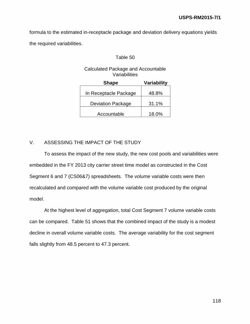
USPS-RM2015-7/1

118

formula to the estimated in-receptacle package and deviation delivery equations yields

the required variabilities.

Table 50

Calculated Package and Accountable Variabilities

Shape Variability

In Receptacle Package 48.8%

Deviation Package 31.1%

Accountable 18.0%

V. ASSESSING THE IMPACT OF THE STUDY

To assess the impact of the new study, the new cost pools and variabilities were

embedded in the FY 2013 city carrier street time model as constructed in the Cost

Segment 6 and 7 (CS06&7) spreadsheets. The volume variable costs were then

recalculated and compared with the volume variable cost produced by the original

model.

At the highest level of aggregation, total Cost Segment 7 volume variable costs

can be compared. Table 51 shows that the combined impact of the study is a modest

decline in overall volume variable costs. The average variability for the cost segment

falls slightly from 48.5 percent to 47.3 percent.

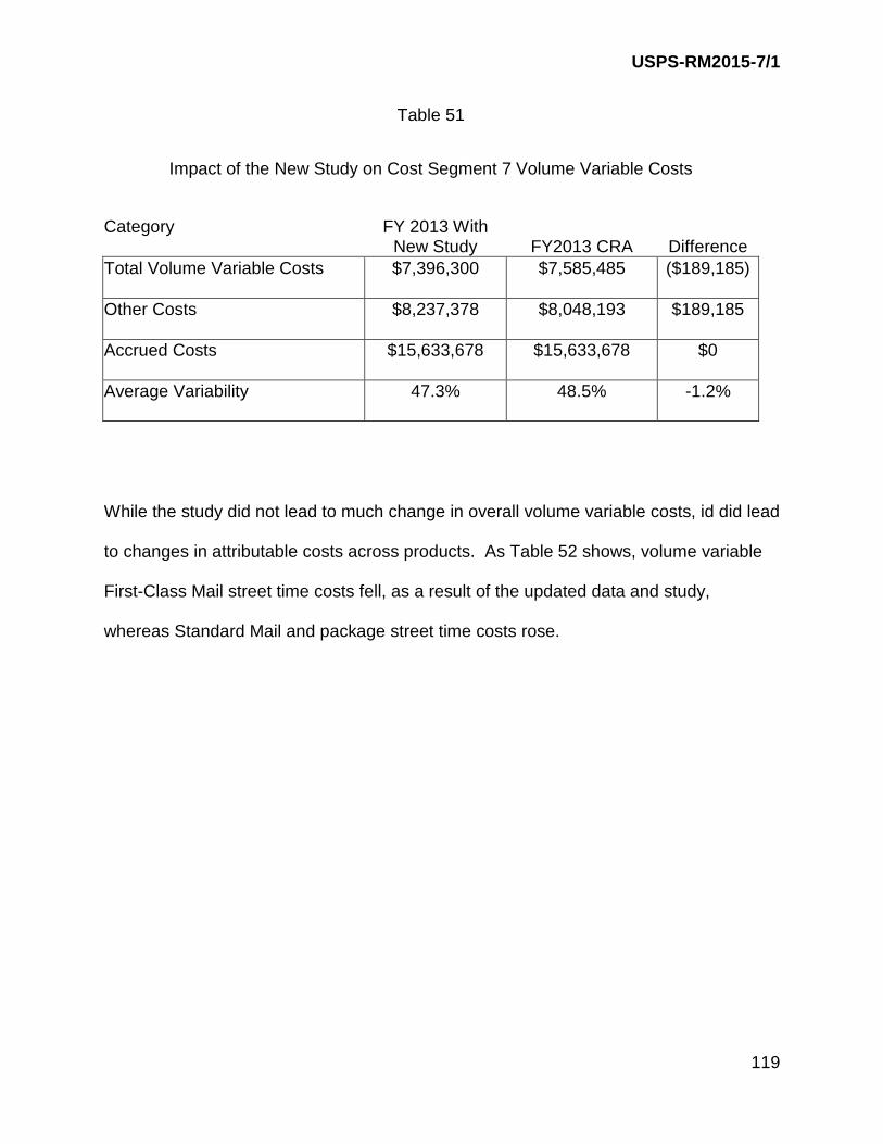
USPS-RM2015-7/1

119

Table 51

Impact of the New Study on Cost Segment 7 Volume Variable Costs

Category FY 2013 With New Study FY2013 CRA Difference

Total Volume Variable Costs $7,396,300 $7,585,485 ($189,185)

Other Costs $8,237,378 $8,048,193 $189,185

Accrued Costs $15,633,678 $15,633,678 $0

Average Variability 47.3% 48.5% -1.2%

While the study did not lead to much change in overall volume variable costs, id did lead

to changes in attributable costs across products. As Table 52 shows, volume variable

First-Class Mail street time costs fell, as a result of the updated data and study,

whereas Standard Mail and package street time costs rose.

USPS-RM2015-7/1

120

These changes are entirely consistent with a decline in First-Class Mail relative

to Standard Mail, and increases in both sequenced mail volume and package volume.

FY 2013 CRA With New Study FY 2013 CRA Difference

FIRST-CLASS MAIL SINGLE-PIECE LETTERS $1,274,692 $1,539,729 ($265,037) SINGLE-PIECE CARDS $71,987 $84,929 ($12,942) PRESORT LETTERS $1,053,440 $1,126,093 ($72,653) PRESORT CARDS $51,451 $54,670 ($3,219) SINGLE PIECE FLATS $149,609 $165,937 ($16,328) PRESORT FLATS $89,062 $89,277 ($215) PARCELS $51,575 $44,015 $7,560STANDARD MAIL HIGH DENSITY & SATURATION LETTERS $145,675 $131,999 $13,676 HIGH DENSITY & SATURATION FLATS & PARCELS $462,102 $280,815 $181,286 EVERY DOOR DIRECT MAIL - RETAIL $36,805 $23,446 $13,359 CARRIER ROUTE $651,512 $588,339 $63,173 LETTERS $1,280,824 $1,381,078 ($100,254) FLATS $562,062 $529,267 $32,795 PARCELS $18,519 $15,114 $3,405PERIODICALS IN COUNTY $30,553 $27,787 $2,766 OUTSIDE COUNTY $421,632 $395,317 $26,315PACKAGE SERVICES BOUND PRINTED MATTER FLATS $19,272 $19,568 ($295) BOUND PRINTED MATTER PARCELS $47,277 $43,698 $3,579 MEDIA AND LIBRARY MAIL $22,697 $20,756 $1,941Ancillary Services CERTIFIED $93,244 $117,738 ($24,494) COD $427 $523 ($96) INSURANCE $4,351 $6,191 ($1,840) REGISTRY $1,150 $1,326 ($176)Competitive ProductsTotal Competitive Products $679,641 $598,167 $81,474

Changes in Volume Variable Street Time Costs by ProductTable 52

USPS-RM2015-7/1

121

Figure 16: Percentage Changes in Delivered Volumes by Shape

Lastly, the impact of the changes in street time volume variable cost on individual

product costs can be assessed by recalculating the overall FY2013 attributable costs

per piece using the new study. Those new costs, along with the FY 2013 costs are

provided in Table 53.

- 15% - 10%

- 5% 0% 5%

10% 15% 20% 25%

Letters Flat

Saturation/ Sequenced Packages

City Carrier Delivered Volume Changes 2010 - 2013

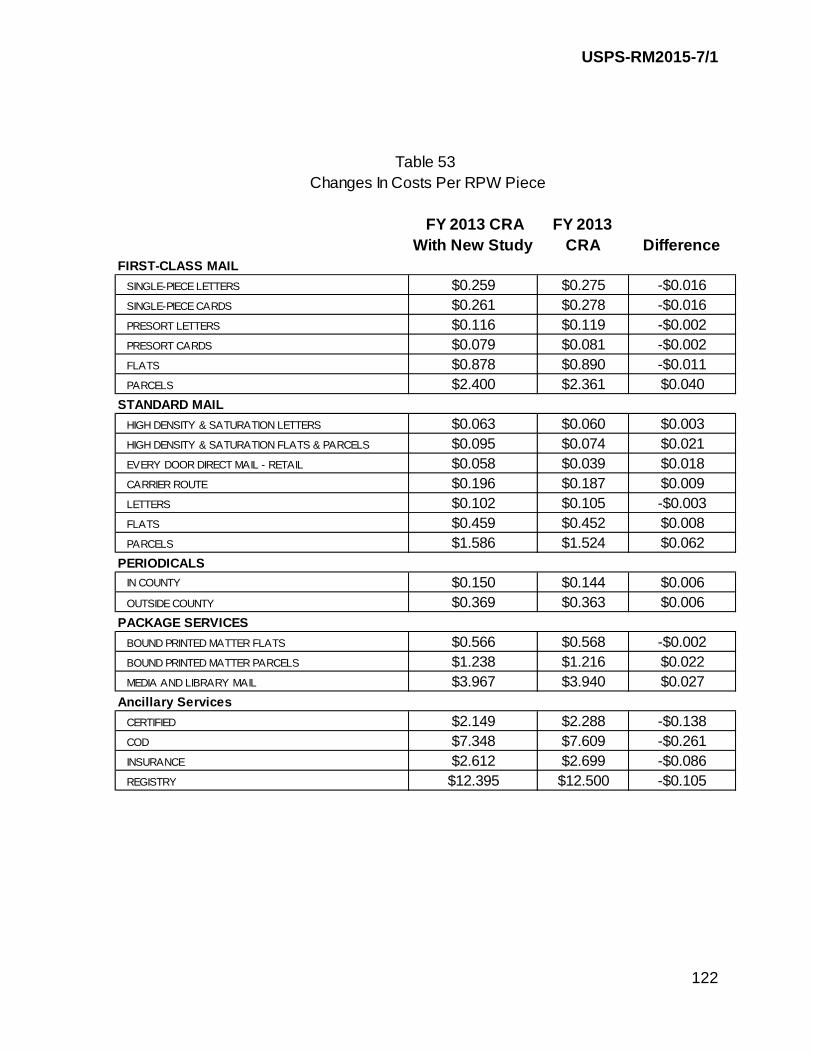
USPS-RM2015-7/1

122

FY 2013 CRA With New Study

FY 2013 CRA Difference

FIRST-CLASS MAIL SINGLE-PIECE LETTERS $0.259 $0.275 -$0.016 SINGLE-PIECE CARDS $0.261 $0.278 -$0.016 PRESORT LETTERS $0.116 $0.119 -$0.002 PRESORT CARDS $0.079 $0.081 -$0.002 FLATS $0.878 $0.890 -$0.011 PARCELS $2.400 $2.361 $0.040STANDARD MAIL HIGH DENSITY & SATURATION LETTERS $0.063 $0.060 $0.003 HIGH DENSITY & SATURATION FLATS & PARCELS $0.095 $0.074 $0.021 EVERY DOOR DIRECT MAIL - RETAIL $0.058 $0.039 $0.018 CARRIER ROUTE $0.196 $0.187 $0.009 LETTERS $0.102 $0.105 -$0.003 FLATS $0.459 $0.452 $0.008 PARCELS $1.586 $1.524 $0.062PERIODICALS IN COUNTY $0.150 $0.144 $0.006 OUTSIDE COUNTY $0.369 $0.363 $0.006PACKAGE SERVICES BOUND PRINTED MATTER FLATS $0.566 $0.568 -$0.002 BOUND PRINTED MATTER PARCELS $1.238 $1.216 $0.022 MEDIA AND LIBRARY MAIL $3.967 $3.940 $0.027Ancillary Services CERTIFIED $2.149 $2.288 -$0.138 COD $7.348 $7.609 -$0.261 INSURANCE $2.612 $2.699 -$0.086 REGISTRY $12.395 $12.500 -$0.105

Changes In Costs Per RPW PieceTable 53