Embed Size (px)
Citation preview

Minor Master Project
Post-Newtonian N-body Dynamics
Author:
Emiel Por
Supervisors:
Simon F. Portegies Zwart
Adrian S. Hamers
October 2014

– 1 –
Post-Newtonian N-body Dynamics
Emiel Por
Abstract
The majority of codes for relativistic N -body simulations fail to take all known first post-
Newtonian order terms in the equations of motion into account for computational reasons. Will
(2014) showed that in some cases, for instance hierarchical systems or systems with a central massive
object, some of the neglected terms are of similar or even higher importance than the terms that
are taken into account, and he provides a way to efficiently calculate the relevant neglected terms,
called cross-terms. We evaluate his method and provide expressions for the cross-terms in the case
of multiple massive objects, yielding terms of similar algorithmic complexity.
We use the Hermite integration scheme and Kustaanheimo-Stiefel regularization in the quater-
nion formation to numerically integrate the full first post-Newtonian equations of motion, in order
to investigate the importance of the neglected terms. The code was validated using both two-body
and hierarchical triple systems, reproducing the osculating elements derived analytically using La-
granges planetary equations, and the resonant eccentricity excitations, induced by post-Newtonian
effects, recently obtained using purely secular orbital averaging methods by Naoz et al. (2013b).
We however failed to reproduce their results for eccentric Kozai mechanism induced purely by
post-Newtonian effects, instead of the usual Newtonian octupole variations, casting doubt on the
existance of such a mechanism.

– 2 –
Contents
1 Introduction 3
1.1 Post-Newtonian Expansion . . . . . . . . . . . . . . . . . . . . . . . . . . . . . . . . 3
1.2 Numerical methods . . . . . . . . . . . . . . . . . . . . . . . . . . . . . . . . . . . . . 4
1.3 Validation . . . . . . . . . . . . . . . . . . . . . . . . . . . . . . . . . . . . . . . . . . 6
1.4 Organisation of this thesis . . . . . . . . . . . . . . . . . . . . . . . . . . . . . . . . . 6
2 Post-Newtonian expansion and cross-terms 7
2.1 Cross-terms for central SMBH . . . . . . . . . . . . . . . . . . . . . . . . . . . . . . . 7
2.2 Cross-terms for multiple central SMBH . . . . . . . . . . . . . . . . . . . . . . . . . 11
3 Numerical methods 15
3.1 Stopping conditions and parallelization . . . . . . . . . . . . . . . . . . . . . . . . . . 16
3.2 Hermite integration . . . . . . . . . . . . . . . . . . . . . . . . . . . . . . . . . . . . . 17
3.3 Regularization . . . . . . . . . . . . . . . . . . . . . . . . . . . . . . . . . . . . . . . 20
4 Validation of the code 26
4.1 Two-body systems . . . . . . . . . . . . . . . . . . . . . . . . . . . . . . . . . . . . . 26
4.2 Kozai-Lidov cycles . . . . . . . . . . . . . . . . . . . . . . . . . . . . . . . . . . . . . 32
4.3 N -body systems . . . . . . . . . . . . . . . . . . . . . . . . . . . . . . . . . . . . . . 40
5 Conclusion and future work 45
Acknowledgements 45
References 47
A EIH equations of motion 50
B Substituting conservation of total linear momentum 51

– 3 –
1. Introduction
1.1. Post-Newtonian Expansion
General relativity was developed by Einstein from 1907 to 1915 (see Weinstein (2012) for an
interesting read on the history of this development) and views gravity as the result of the curvature
of space-time. The Einstein field equations dictate the gravitational interaction between particles,
but these equations are non-linear and therefore notoriously hard to solve. Schwarzschild (1916)
found the first non-trivial solution to the Einstein field equations: the Schwarzschild metric, which
describes a Schwarzschild black hole, a point-like massive particle.
One can make several expansions to the field equations to make solving them easier. One
of these expansions is now known as the post-Newtonian (PN) expansion, which expands the
gravitational field in terms of v/c, where v is the typical velocity of a particle and c is the speed
of light. In this expansion an exact solution (to first non-zero order: v2/c2) for the motion of N
Schwarzschild black holes was found by Einstein et al. (1938). The resulting equations of motion
for the particles are known as the Einstein-Infeld-Hoffman (EIH) equations of motion and are
aa =−∑b 6=a
Gmbxab
r3ab
+1
c2
∑b 6=a
Gmbxab
r3ab
4Gmb
rab+ 5
Gma
rab+∑c 6=a,b
Gmc
rbc
+4∑c 6=a,b
Gmc
rac− 1
2
∑c 6=a,b
Gmc
r3bc
(xab · xbc)− v2a + 4va · vb − 2v2
b +3
2(vb · nab)
2
− 7
2c2
∑b 6=a
Gmb
rab
∑c 6=a,b
Gmcxbc
r3bc
+1
c2
∑b 6=a
Gmb
r3ab
xab · (4va − 3vb)vab, (1)
where:
(2a)nab =xab
rab,
(2b)vab = va − vb ,
(2c)xab = xa − xb ,
(2d)rab = |xab| ,
(2e)va = |va| .
This equation of motion permits a conserved total energy and total linear momentum, which can be
found in Appendix A. The zeroth-order term in this equation of motion is the standard Newtonian
term, the others are post-Newtonian correction terms, some dependent on the velocity of the
particles. The second to last term originally contains the acceleration of other particles, making it
harder to solve the accelerations of all particles simultaniously. A common approximation, as also
applied to Equation A1, is to substitute the Newtonian acceleration, as higher order post-Newtonian
corrections to this acceleration create second-order corrections to the acceleration.

– 4 –
Higher order post-Newtonian corrections exist, but not for an arbitrary number of particles.
The three-body Hamiltonian, and therefore the corresponding equations of motion, is known in
closed form to second post-Newtonian order (O(v4/c4
)), see Schafer (1987) and Lousto and Nakano
(2008), the latter of which corrects typos made by the first. The two-body equations of motion are
known to as far as 3.5PN order, O(v7/c7
), of which the 2.5PN terms show the interesting feature
of energy loss via gravitational waves, as recently derived by Futamase and Itoh (2007) and Itoh
(2009).
Note that Equation A1 also contains summations over pairs of bodies, so the motion of one
particle due to a second particle is dependent on their surroundings, which is not the case for
Newtonian gravity. Curiously, note that it only contains summations of pairs of particles, but not
over triples of more particles, as the non-linearity of the Einstein field equations would suggest.
This makes the equations of motion for one particle O(N2), and therefore evaluation of all particles
O(N3).
Even though this is better than O(NN
), it is still prohibitive to do simulations for large
numbers of particles. Most post-Newtonian implementations discard all summations of pairs of
particles for computational reasons. The discarded terms are however of the same order as the
terms that are not discarded, and the integrated equations of motion do not completely satisfy
general relativity.
A better way of discarding unnecessary terms was introduced by Will (2014). He used an
additional second expansion in a small parameter defined by the physical problem that we want to
solve. In the case of stars orbiting a central supermassive black hole (SMBH), we can use m/M
as our small parameter, where m is the typical mass of a star and M is the mass of the SMBH.
In the case of a hierarchical three-body problem, we can use a1/a2 where a1, a2 are the semimajor
axes of the inner and the outer binary respectively. Will (2014) showed that an expansion in this
way generally leaves summations over pairs of particles in the highest order terms, which can then
be discarded without compromising agreement with general relativity too much. The second-to-
highest order terms mostly contain select terms in the summations over pairs of particles and can
therefore be efficiently evaluated; these terms are called cross-terms by Will (2014). In a second
paper on the subject, Will (2014) showed that the total energy and total angular momentum in
hierarchical triple systems, is only conserved to Newtonian order, if and only if the cross-terms
are taking into account when integrating the system. Other than the search for completeness,
this makes cross-terms an interesting branch of post-Newtonian stellar dynamics in current-day
research.
1.2. Numerical methods
Solving the equations of motion for an arbitrary N -body system, that is, finding the positions
and velocities for all particles at a later time t1 given the positions and velocities at an initial time

– 5 –
t0, is done using numerical integration techniques. Of these techniques the Hermite integration
scheme (Makino 1991), a family of higher order variants on the leapfrog scheme, is arguably the
most used in modern computational astrophysics. In spite of its good performance, close encounters
of two particles, such as those generated by highly eccentric binaries due to Kozai-Lidov cycles,
still generate significant integration errors, which can be mitigated, but requires decreasing the
timestep and therefore increasing the computation time. The integration scheme is not to blame
for this kind of problem, but rather of the existance of a singularity in the Newtonian equations
of motion themselves: in the extreme case that the particles collide exactly, the distance between
those particles is zero and the acceleration is infinite/undefined, therefore making it harder for any
integration scheme to integrate through close encounters.
One possible solution to this problem is to rewrite the equations of motion in such a coordinate
system that the singularity disappears. This technique, known as regularization, was most famously
applied on the 3D Keplerian problem by Kustaanheimo and Stiefel (1965). Kustaanheimo-Stiefel
regularization (hereafter KS-regularization) introduces regularized time and space coordinates, in
which the equation of motion for an unperturbed binary reduces to a harmonic oscillator, void
of singularities. Perturbations to the regularized binary correspond to a perturbed harmonic os-
cillator, making it easy to integrate close encounters, while other particles are still integrated in
unregularized coordinates. In addition, as KS-regularization only accounts for the Newtonian ac-
celeration between the regularized particles, post-Newtonian terms also act as a perturbation on
the binary. A relatively new formulation of KS-regularization was introduced by Waldvogel (2006),
who uses quaternions, an extension to complex numbers, to write the KS-transformation in a more
concise and elegant formulation than the more common KS-matrix transformation.
Due to the success of KS-regularization, many types of regularization were developed, regular-
izing the three-body system using two KS-transformations (Aarseth and Zare 1974), regularizing
a whole chain of an arbitrary number of particles (Mikkola and Aarseth 1989), and pairwise reg-
ularization of an arbitrary number of particle with a central particle (Zare 1974). The latter is
perfectly suited for particles orbiting a central massive particle, as is the case in the galactic center
for stars and a SMBH. Aarseth (2007) showed for the first time a large scale simulation, N ∼ 105
particles, using this regularization technique, which looks promising.
Hut et al. (1995) showed that time-symmetric integrators are to be prefered compared to non-
time-symmetric ones, due to their inherent energy conservation properties. Although the Hermite
scheme is time-symmetric (symplectic) when using a constant timestep, the use of a non-time-
symmetric timestep spoils this time-symmetry and again results in drifting of otherwise conserved
quantities.
In this thesis we have implemented a Hermite integrator using KS-regularization for close
encounters. Post-Newtonian terms can be added, including all terms in the EIH equations of
motion. The code was directly developed in AMUSE (Portegies Zwart et al. 2013; Pelupessy et al.
2013), which allows direct comparison and validation with other codes, such as an arbitrary precision

– 6 –
Newtonian code based on a Bulirsch-Stoer integrator, Brutus (Portegies Zwart and Boekholt 2014),
Hermite, based on Hut et al. (1995), MI6, based on Nitadori and Makino (2008) and Iwasawa et al.
(2011), and ARCHAIN (Mikkola and Merritt 2008).
1.3. Validation
To validate the developed code, we first investigate the accuracy of the integrator by comparing
integrations with varying timestep parameter to analytical solutions in the non-relativistic two-body
problem. We then extend this analysis to the relativistic two-body problem, using the theory of
Lagrange planetary equations as the analytical solution, cf. Merritt (2013), .
We extend our validation to the hierarchical three-body problem, in which we can differentiate
a close binary and a third body that orbits that binary. We show numerical simulations in the
case of non-relativistic triples, reproducing the famous quadrupole Kozai-Lidov cycles discovered
by Lidov (1962) and Kozai (1962). In addition we simulate triples in which the next order, the
octupole level variations, become important and show the resulting orbital flips found by Naoz
et al. (2013a), which can increase the inner binary eccentricity to extremely high values (up to
1− e1 ∼ 10−7 in some cases).
We then investigate the result of post-Newtonian corrections to Kozai cycles, reproducing
the resonant-like eccentricity excitation discovered by Naoz et al. (2013b), using direct numerical
integrations instead of ones using secular approximations. Furthermore, we reproduce the orbital
flips induced by post-Newtonian corrections, even when the octupole-level variations, the usual
cause for orbital flips, are insigificant.
We then apply our code to the problem of stellar dynamics around a super-massive black
hole. We use a slight variation on the initial conditions by Hamers et al. (2014) to describe the
general performance of our code. We show the runtime scaling of our perturbations (O(N2)
for
perturbations, except for the EIH equations of motion which has order O(N3)), the runtime scaling
for the number of computation cores used, and the energy behaviour as a function of timestep
parameter. Based on these results it is possible to determine the required timestep parameter and
resulting wall-clock time for simulations.
1.4. Organisation of this thesis
In Section 2 we rederive the expressions for the post-Newtonian cross-terms for stellar cluster
with a central massive object, and extend his analysis to multiple massive objects. In Section 3 we
explicitly write down all numerical methods used in the developed code, to give an insight in the
inner workings, and potential numerical errors. In Section 4 we validate the code using analytical
solutions and approximations for the (non)-relativistic two-body, and hierarchical triple systems.

– 7 –
In Section 5 we give the conclusion of this thesis and provide possible options for future work.
2. Post-Newtonian expansion and cross-terms
In this section we will redo the first derivation of cross-terms done by Will (2014) more ex-
plicitly, which describes the case of a stellar cluster with a central massive object. Then, we will
extend his derivation by allowing multiple massive objects, resulting in expressions for the cross-
terms of identical nature (same order expansion) and algorithmic complexity (also of O(N2)
for
the calculation of all accelerations).
2.1. Cross-terms for central SMBH
We now look more closely at the situation of a central supermassive black hole (SMBH) sur-
rounded by stellar mass black holes. In this case, the mass ratio m/M 1, where m is the typical
mass of a star and M is the mass of the SMBH, provides an excellent small parameter to base
the order expansion on. This situation is the first that Will (2014) uses as a case study when
introducing cross-terms. In this seciton, we will redo his derivation somewhat more explicitly.
2.1.1. Equation of motion for the central SMBH
We will denote the black hole as particle 1, so m1 = M ma for a 6= 1. We start by deriving
the equations of motion for the SMBH. The EIH equations of motion written out for the black hole
are
a1 =−∑b 6=1
Gmbx1b
r31b
+1
c2
∑b 6=1
Gmbx1b
r31b
4Gmb
r1b+ 5
GM
r1b+∑c 6=1,b
Gmc
rbc
+4∑c 6=1,b
Gmc
r1c− 1
2
∑c 6=1,b
Gmc
r3bc
(x1b · xbc)− v21 + 4v1 · vb − 2v2
b +3
2(vb · n1b)
2
− 7
2c2
∑b 6=1
Gmb
r1b
∑c 6=1,b
Gmcxbc
r3bc
+1
c2
∑b 6=1
Gmb
r31b
x1b · (4v1 − 3vb)v1b.
(3)
As m M , where m is the typical mass of a star, this equation contains terms with different
orders of magnitude. We can reorder these terms like
a1 = −∑b 6=1
Gmbx1b
r31b
+1
c2[a1]BH +
1
c2[a1]Cross +
1
c2[a1]Rest, (4)
where each of the terms have a specific order. The first term is Newtonian gravity of order O(Gmr2
);
the other three are the 1PN corrections of order O(G2M2
c2r3
(mM
)i)where i = 1, 2, 3 for the second,

– 8 –
third and fourth order respectively. The velocity dependent terms can also be graded into the same
orders: v1 ∼ mM v and v2 ∼ GM
r , where v is the typical velocity of a star and r is the typical distance
between star and the SMBH. These orders of the velocities are justified when the motion of the
star is dominated by the black hole.
The reordering results in
[a1]BH =∑b 6=1
Gmbx1b
r31b
(5GM
r1b− 2v2
b +3
2(vb · n1b)
2
)+ 3
∑b 6=1
Gmb
r31b
(vb · x1b)vb, (5)
[a1]Cross = 4∑b6=1
G2m2bx1b
r41b
+∑b 6=1
∑c 6=1,b
G2mbmcx1b
r31b
(4
r1c+
5
4rbc− r2
1c
4r3bc
+r2
1b
4r3bc
)− 7
2
∑b 6=1
Gmb
r1b
∑c 6=1,b
Gmcxbc
r3bc
+∑b 6=1
Gmb
r31b
[4(v1 · vb)x1b − 3(vb · x1b)v1 − 4(vb · x1b)vb] , (6)
[a1]Rest = O(G2m3
Mc2r3
), (7)
where we have used that:
−1
2x1b · xbc =
1
4(r2
bc + r21b − r2
1c). (8)
2.1.2. Equations of motion for the stars
The equations of motion for stars are a little more elaborate to derive, as the terms in the
EIH equations of motion cannot be simply reordered. The EIH equations of motion written out for
stars are
aa =−∑b 6=a
Gmbxab
r3ab
+1
c2
∑b 6=a
Gmbxab
r3ab
4Gmb
rab+ 5
Gma
rab+∑c 6=a,b
Gmc
rbc
+4∑c 6=a,b
Gmc
rac− 1
2
∑c 6=a,b
Gmc
r3bc
(xab · xbc)− v2a + 4va · vb − 2v2
b +3
2(vb · nab)
2
− 7
2c2
∑b 6=a
Gmb
rab
∑c 6=a,b
Gmcxbc
r3bc
+1
c2
∑b 6=a
Gmb
r3ab
xab · (4va − 3vb)vab,
(9)
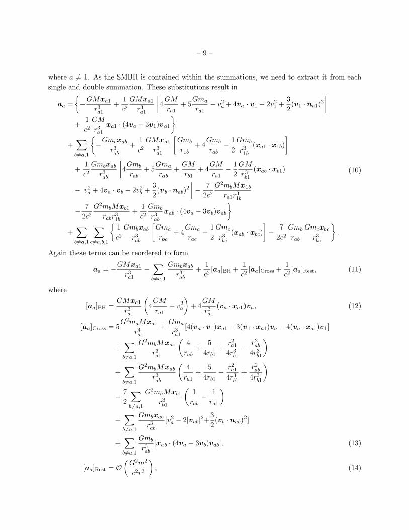
– 9 –
where a 6= 1. As the SMBH is contained within the summations, we need to extract it from each
single and double summation. These substitutions result in
aa =
−GMxa1
r3a1
+1
c2
GMxa1
r3a1
[4GM
ra1+ 5
Gma
ra1− v2
a + 4va · v1 − 2v21 +
3
2(v1 · na1)2
]+
1
c2
GM
r3a1
xa1 · (4va − 3v1)va1
+∑b 6=a,1
−Gmbxab
r3ab
+1
c2
GMxa1
r3a1
[Gmb
r1b+ 4
Gmb
rab− 1
2
Gmb
r31b
(xa1 · x1b)
]
+1
c2
Gmbxab
r3ab
[4Gmb
rab+ 5
Gma
rab+GM
rb1+ 4
GM
ra1− 1
2
GM
r3b1
(xab · xb1)
− v2a + 4va · vb − 2v2
b +3
2(vb · nab)
2
]− 7
2c2
G2mbMx1b
ra1r31b
− 7
2c2
G2mbMxb1
rabr31b
+1
c2
Gmb
r3ab
xab · (4va − 3vb)vab
+∑b 6=a,1
∑c 6=a,b,1
1
c2
Gmbxab
r3ab
[Gmc
rbc+ 4
Gmc
rac− 1
2
Gmc
r3bc
(xab · xbc)
]− 7
2c2
Gmb
rab
Gmcxbc
r3bc
.
(10)
Again these terms can be reordered to form
aa = −GMxa1
r3a1
−∑b 6=a,1
Gmbxab
r3ab
+1
c2[aa]BH +
1
c2[aa]Cross +
1
c2[aa]Rest, (11)
where
[aa]BH =GMxa1
r3a1
(4GM
ra1− v2
a
)+ 4
GM
r3a1
(va · xa1)va, (12)
[aa]Cross = 5G2maMxa1
r4a1
+Gma
r3a1
[4(va · v1)xa1 − 3(v1 · xa1)va − 4(va · xa1)v1]
+∑b 6=a,1
G2mbMxa1
r3a1
(4
rab+
5
4rb1+
r2a1
4r3b1
−r2ab
4r3b1
)
+∑b 6=a,1
G2mbMxab
r3ab
(4
ra1+
5
4rb1− r2
a1
4r3b1
+r2ab
4r3b1
)
− 7
2
∑b6=a,1
G2mbMxb1
r3b1
(1
rab− 1
ra1
)+∑b 6=a,1
Gmbxab
r3ab
[v2a − 2|vab|2+
3
2(vb · nab)
2]
+∑b 6=a,1
Gmb
r3ab
[xab · (4va − 3vb)vab], (13)
[aa]Rest = O(G2m2
c2r3
), (14)

– 10 –
where we have used that
(15a)−v2a + 4va · vb − 2v2
b = v2a − 2|vab|2 ,
(15b)12xa1 · xb1 = 1
4(r2b1 + r2
a1 − r2ab) ,
(15c)−12xab · xb1 = 1
4(r2b1 − r2
a1 + r2ab) .
The first two terms in Equation 11 are Newtonian: O(GMr2
)and O
(Gmr2
)respectively. The other
three terms are PN corrections of order O(G2M2
c2r3
(mM
)i)where i = 0, 1, 2 for the third, fourth and
fifth term respectively.
Note that all double summation terms in the original expression for the equations of motion of
the stars correspond to rest terms therefore belong to the highest order terms in the equations of
motion. We can therefore leave these highest order corrections out to have no double summations
in our final expression and have a O(N2)
algorithm for calculating all accelerations (both of the
stars and single SMBH) instead of the O(N3)
algorithm using the EIH equations of motion. Notice
that there are double summations in the equations of motion for the SMBH, but as there is only
one SMBH this doesn’t change the complexity of the calculations.
Truncating the equations of motion in this way does not correspond to leaving out all double
summations in the EIH. The cross terms still contain the important double summations, namely
those over all two stars and the SMBH. This intuitive way of visualisation shouldn’t be taken to
extremes, as the only discriminator is the order of those terms and not their origin. In fact, some
of the PN terms between a star and a SMBH, and some of the double summation terms in triples
consisting of two stars and the SMBH are still left out, while some of the PN terms between two
stars are still included in the cross-terms. Also note that to consistently truncate the equations of
motion, we need to calculate those of the SMBH to order mM higher than those of the stars. This
makes sense as v1 ∼ mM v.
These equations of motion are equivalent to the expressions derived by Will (2014), after
substitution of conservation of linear momentum to Newtonian order
v1 = −∑a6=1
ma
Mva. (16)
Substitution of conservation of linear momentum up to first post-Newtonian order is not necessary,
as all velocity dependent terms are first post-Newtonian order themselves, making the corrections
in linear momentum second post-Newtonian order. This substitution is not trivial and is done in
Appendix B.

– 11 –
2.1.3. Energy and linear momentum
The expressions for the conserved quantities energy and linear momentum can also be derived
in the same way. We again extract the black hole from each summation, and make an order
expansion as above. This leads to the following expressions for energy and linear momentum:
E =1
2Mv2
1 +1
2
∑a6=1
mav2a −
∑a6=1
GMma
ra1− 1
2
∑a6=1
∑b6=a,1
Gmamb
rab
+1
c2
3
8
∑a6=1
mav4a +
3
2
∑a6=1
GMmav2a
ra1+
1
2
∑a6=1
G2M2ma
r21a
+1
4
∑a6=1
∑b6=a,1
Gmamb
rab
[6v2
a − 7va · vb − (va · nab)(vb · nab)]
+1
2
∑a6=1
GMma
ra1
[3v2
1 − 7v1 · va − (v1 · na1)(va · na1)]
+∑a6=1
∑b 6=a,1
G2Mmamb
rabra1+
1
2
∑a6=1
∑b6=1
G2Mmamb
r1ar1b
+O(G2m3
c2r2
),
(17)
and
P = Mv1 +∑a6=1
mava +1
2c2
∑a6=1
mav2ava −
∑a6=1
GMma
ra1[va + (va · na1)na1]
−∑a6=1
GMma
ra1[v1 + (v1 · na1)na1]−
∑a6=1
∑b6=a,1
Gmamb
rab[va + (va · nab)nab]
+O
(Gm3v
Mr
).
(18)
Note that in the last term of Equation 17, star b can be star a, which is not clear in Will (2014)
due to his notation of summations.
2.2. Cross-terms for multiple central SMBH
For various reasons it is interesting to look at a slight variation on the situation described
above. One of which is the mergers of galaxies, as most, if not all, galactic cores contain a SMBH,
leading to multiple SMBHs in the simulation. However, observational evidence (Schnittman 2013)
suggests that these SMBHs must coalesce on a relatively short timescale, as we see far too little
SMBH binaries in the sky. In theory however, this coalescence takes too long to explain the low
number of SMBH binaries found in the sky, leading to the famous final parsec problem, as first
stated by Begelman et al. (1980). In current research, three main phases are differentiated in
galactic mergers:

– 12 –
1. As galaxies collide, the black holes fall to the center of the potential well of the stars as the
result of dynamical friction.
2. As the two SMBHs lose enough velocity they form a hard binary and start to scatter single
stars via three-body scattering. However, the stars have to be in the loss cone to be scattered
by the SMBH binary, which is the region in (L,E) phase space where the pericenter distance
of stars is close enough to the SMBH binary to be scattered. When the loss cone is empty, no
stars orbit close enough to the binary to be scattered. Refilling of the loss cone is possible via
orbital perturbations of the orbits of the stars due to interactions with the galaxy potential
or via (non)-collisional interactions between stars directly, but studies to date show that this
refilling is too slow to reach the third and final phase on a sufficiently short timescale.
3. The SMBHs now orbit close enough to radiate significant amounts of energy away via gravi-
tational waves and finaly coalesce.
Various solutions for the final parsec problem have bee n proposed (eg. Lodato et al. (2009);
Khan et al. (2011, 2013); Vasiliev et al. (2014)), but none provide a sufficient or satisfiable solution.
New terms in the equations of motion of stars around such a SMBH binary would provide a possible
solution, if they cause more chaotic orbits, therefore increasing the relaxation rate of the stars, in
return creating a higher refilling rate of the loss cone. Cross-terms could provide such terms, as
commonly the two-body summations in the EIH equations of motion are not taken into account in
current simulations. These (cross) terms are of order O(G2M2
c2r3
)and therefore of the highest order
PN terms for stars. However, it is still an open question if these terms significantly impact the
evoluton of orbits near the SMBH binary.
When deriving the cross terms in this slightly different situation, we need to take care when
evaluating the order of velocity dependent terms, as a SMBH don’t have a velocity of order V ∼ mM v
anymore, but instead order V ∼ v, which makes the number of cross-terms a bit higher than before.
In this derivation, we indicate all SMBHs by upper case indices, and the lower mass black holes by
lower case ones. As before we expand each summation over all particles into two summations, one
over all SMBHs and one over all lower mass BHs. This leads to the following equations of motion

– 13 –
for one of the SMBHs:
aA = −∑B 6=A
GmBxAB
r3AB
−∑b
GmbxAb
r3Ab
+1
c2
∑B 6=A
GmBxAB
r3AB
4GmB
rAB+ 5
GmA
rAB+
∑C 6=A,B
GmC
rBC+∑c
Gmc
rBc+ 4
∑C 6=A,B
GmC
rAC
+4∑c
Gmc
rAc− 1
2
∑C 6=A,B
GmC
r3BC
(xAB · xBC)− 1
2
∑c
Gmc
r3Bc
(xAB · xBc)
−v2A + 4vA · vB − 2v2
B +3
2(vB · nAB)2
]
+1
c2
∑b
GmbxAb
r3Ab
4Gmb
rAb+ 5
GmA
rAb+∑C 6=A
GmC
rbC+∑c 6=b
Gmc
rbc+ 4
∑C 6=A
GmC
rAC
+4∑c 6=b
Gmc
rAc− 1
2
∑C 6=A
GmC
r3bC
(xAb · xbC)− 1
2
∑c 6=b
Gmc
r3bc
(xAb · xbc)
−v2A + 4vA · vb − 2v2
b +3
2(vb · nAb)
2
]
− 7
2c2
∑B 6=A
GmB
rAB
∑C 6=A,B
GmCxBC
r3BC
+∑c
GmcxBc
r3Bc
− 7
2c2
∑b
Gmb
rAb
∑C 6=A
GmCxbC
r3bC
+∑c6=b
Gmcxbc
r3bc
+
1
c2
∑B 6=A
GmB
r3AB
xAB · (4vA − 3vB)vAB +∑b
Gmb
r3Ab
xAb · (4vA − 3vb)vAb
.
(19)
The equations of motion for one of the stars are derived analogously, resulting in the same
expression as above, save for the exchange of upper and lower case indices, due to the symmetry
in the derivation. These two expanded expressions can be reordered as
aA = −∑B 6=A
GmBxAB
r3AB
−∑b
GmbxAb
r3Ab
+1
c2[aA]BH +
1
c2[aA]Cross +
1
c2[aA]Rest, (20)
aa = −∑B
GmBxaB
r3aB
−∑b 6=a
Gmbxab
r3ab
+1
c2[aa]BH +
1
c2[aa]Cross +
1
c2[aa]Rest, (21)
where the first two terms in each equation of motion are Newtonian order, O(GMr2
)and O
(Gmr2
)respectively, and the three other terms post-Newtonian order, O
(G2M2
c2r3
(mM
)i)where i = 0, 1, 2
respectively. The subexpressions are:

– 14 –
(22a)
[aA]BH =∑B 6=A
GmBxAB
r3AB
4GmB
rAB+ 5
GmA
rAB+ v2
A
− 2|vAB|2 +3
2(vB · nAB)2 +
∑C 6=A,B
GmC
(1
rBC+
4
rAC− 1
2
xAB · xBC
r2BC
)− 7
2
∑B 6=A
GmB
rAB
∑C 6=A,B
GmCxBC
r3BC
+∑B 6=A
GmB
r3AB
xAB · (4vA − 3vB)vAB ,
(22b)
[aA]Cross =∑B 6=A
GmBxAB
r3AB
∑c
Gmc
(1
rBc+
4
rAc− 1
2
xAB · xBc
r3Bc
)+∑b
GmbxAb
r3Ab
5GmA
rAb+ v2
A
− 2|vAB|2 +3
2(vb · nAb)
2 +∑C 6=A
GmC
(1
rbC+
4
rAC− 1
2
xAb · xbC
r3bC
)− 7
2
∑B 6=A
∑c
G2mBmcxBc
r3Bc
(1
rAB− 1
rAc
)+∑b
Gmb
r3Ab
xAb · (4vA − 3vb)vAb ,
(22c)[aA]Rest = O(G2m2
c2r3
),
and
(23a)
[aa]BH =∑B
GmBxaB
r3aB
4GmB
raB+ v2
a
− 2|vaB|2 +3
2(vB · naB)2 +
∑C 6=B
GmC
(1
rBC+
4
raC− 1
2
xaB · xBC
r3BC
)− 7
2
∑B
GmB
raB
∑C 6=B
GmCxBC
r3BC
+∑B
GmB
r3aB
xaB · (4va − 3vB)vaB ,
(23b)
[aa]Cross =∑B
GmBxaB
r3aB
5Gma
raB+∑c 6=a
Gmc
(1
rBc+
4
rac− 1
2
xaB · xBc
r3Bc
)+∑b 6=a
Gmbxab
r3ab
[v2a − 2|vab|2 +
3
2(vb · naB)2 +
∑C
GmC
(1
rbC+
4
rac− 1
2
xab · xbC
r3bC
)]
− 7
2
∑B
∑c 6=a
G2mBmcxBc
r3Bc
(1
raB− 1
rac
)+∑b 6=a
Gmb
r3ab
xab · (4va − 3vb)vab ,
– 15 –
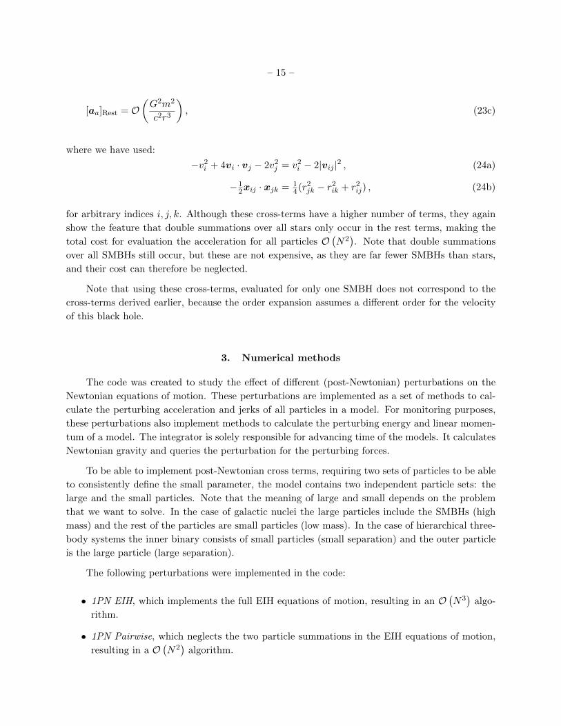
(23c)[aa]Rest = O(G2m2
c2r3
),
where we have used:
(24a)−v2i + 4vi · vj − 2v2
j = v2i − 2|vij |2 ,
(24b)−12xij · xjk = 1
4(r2jk − r2
ik + r2ij) ,
for arbitrary indices i, j, k. Although these cross-terms have a higher number of terms, they again
show the feature that double summations over all stars only occur in the rest terms, making the
total cost for evaluation the acceleration for all particles O(N2). Note that double summations
over all SMBHs still occur, but these are not expensive, as they are far fewer SMBHs than stars,
and their cost can therefore be neglected.
Note that using these cross-terms, evaluated for only one SMBH does not correspond to the
cross-terms derived earlier, because the order expansion assumes a different order for the velocity
of this black hole.
3. Numerical methods
The code was created to study the effect of different (post-Newtonian) perturbations on the
Newtonian equations of motion. These perturbations are implemented as a set of methods to cal-
culate the perturbing acceleration and jerks of all particles in a model. For monitoring purposes,
these perturbations also implement methods to calculate the perturbing energy and linear momen-
tum of a model. The integrator is solely responsible for advancing time of the models. It calculates
Newtonian gravity and queries the perturbation for the perturbing forces.
To be able to implement post-Newtonian cross terms, requiring two sets of particles to be able
to consistently define the small parameter, the model contains two independent particle sets: the
large and the small particles. Note that the meaning of large and small depends on the problem
that we want to solve. In the case of galactic nuclei the large particles include the SMBHs (high
mass) and the rest of the particles are small particles (low mass). In the case of hierarchical three-
body systems the inner binary consists of small particles (small separation) and the outer particle
is the large particle (large separation).
The following perturbations were implemented in the code:
• 1PN EIH, which implements the full EIH equations of motion, resulting in an O(N3)
algo-
rithm.
• 1PN Pairwise, which neglects the two particle summations in the EIH equations of motion,
resulting in a O(N2)
algorithm.
– 16 –
• 1PN GC Crossterms, which implements the cross terms in the case of galactic nuclei derived
in section 2.1.
We also implemented the following integrators:
• Hermite, which uses a standard Hermite integrator with variable but shared time step (Makino
1991).
• SymmetrizedHermite, which is a variant of Hermite, but uses a time-symmetric time step
(Hut et al. 1995).
• RegularizedHermite, which regularizes close approaches of two particles using Kustaanheimo-
Stiefel regularization (Kustaanheimo and Stiefel 1965), still using the standard Hermite
scheme for all time integrations.
• SymmetrizedRegularizedHermite, which is again a variant of RegularizedHermite, but uses a
symmetrized time step (Funato et al. 1996).
In section 3.1 we will describe the way collisions between particles are detected and several other
stopping conditions are implemented. This section also describes how the code uses parallelization
to take advantage of multicore machines. In section 3.2 we will reproduce the equations for Hermite
integration in the Predict, Evaluate and Correct (PEC) formulation. We will also describe the
way the jerks are calculated when explicit, analytical calculation of the jerks is computationally
inefficient. In section 3.3 we will describe the basis of regularization in the language of quaternions,
an extension of the complex numbers, and the regularization of the perturbed two-body problem.
As regularization uses a regularized time, we will also describe the transformation of time steps
between model and regularized time.
3.1. Stopping conditions and parallelization
In the code, all particles have a radius to allow checking for collisions between particles. Within
each integration step, we assume that the particles move in straight lines given by
x(s) = xb + s (xe − xb), (25)
where xb and xe are the positions at the begining and end of the current time step respectively, and
s ∈ [0, 1) a parameter. If the relative distance between two particles is less then the sum of their
radii, for some value of s, we detect a collision and abort model evolution. The collision is then
handled appropriately by the script that runs the simulation, and the simulation can be continued.
The code also supports two other stopping conditions, namely:

– 17 –
• Wall-clock time-out detection, which aborts evolution when the code takes to long on the
wall-clock to evolve to the required model time.
• Maximum number of integration steps detection, which aborts evolution when the evolution
to the required model time takes more than a N integration steps. N can be set by the script.
Parallelization in the code is implemented by the integrators. Multithreading was chosen as
the method of parallelization because of the following reasons:
• Ease of implementation. Communication between threads can be done primarily using shared
memory, and as of C++11 threads are implemented in the standard library making multi-
threading intrinsically cross-platform.
• Small number of particles. This is enforced because comparison with the EIH equations of
motion of O(N3)
is required. A small number of particles means that parallelizing to more
than a few cores is inefficient and it makes communication overhead between cores a critical
factor.
3.2. Hermite integration
3.2.1. PEC scheme
The Hermite integration scheme is a family of implicit numerical methods for solving ordinary
differential equations, and were introduced by Makino (1991). The fourth order variant of this
integration scheme is
y(t+ h) = y(t) +y(1)(t) + y(1)(t+ h)
2h+
y(2)(t)− y(2)(t+ h)
12h2 +O
(h5), (26)
which has a local truncation error of O(h5)
and therefore a global truncation error of O(h4).
Sixth and eight order integration schemes were derived by Nitadori and Makino (2008). As this
integration method is implicit, we need to use fixed-point iteration to solve Equation 26, that is:
y[i+1](t+ h) = y(t) +y(1)(t) + y
(1)[i] (t+ h)
2h+
y(2)(t)− y(2)[i] (t+ h)
12h2, (27)
using a truncated Taylor expansion around t as the initial condition
y[0](t+ h) = y(t) + hy(1)(t) +h2
2y(2)(t). (28)
When this sequence converges, its limit is taken to be y(t+h), and the current time step has ended.
In practice only one iteration is sufficient, as we can reduce integration errors by choosing the time
step h smaller.
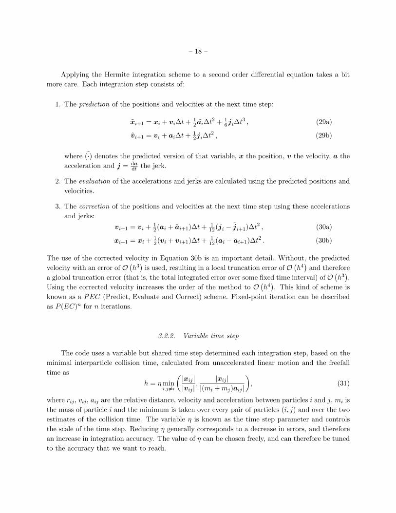
– 18 –
Applying the Hermite integration scheme to a second order differential equation takes a bit
more care. Each integration step consists of:
1. The prediction of the positions and velocities at the next time step:
(29a)xi+1 = xi + vi∆t+ 12 ai∆t
2 + 16ji∆t
3 ,
(29b)vi+1 = vi + ai∆t+ 12ji∆t
2 ,
where (·) denotes the predicted version of that variable, x the position, v the velocity, a the
acceleration and j = dadt the jerk.
2. The evaluation of the accelerations and jerks are calculated using the predicted positions and
velocities.
3. The correction of the positions and velocities at the next time step using these accelerations
and jerks:
(30a)vi+1 = vi + 12(ai + ai+1)∆t+ 1
12(ji − ji+1)∆t2 ,
(30b)xi+1 = xi + 12(vi + vi+1)∆t+ 1
12(ai − ai+1)∆t2 .
The use of the corrected velocity in Equation 30b is an important detail. Without, the predicted
velocity with an error of O(h3)
is used, resulting in a local truncation error of O(h4)
and therefore
a global truncation error (that is, the total integrated error over some fixed time interval) of O(h3).
Using the corrected velocity increases the order of the method to O(h4). This kind of scheme is
known as a PEC (Predict, Evaluate and Correct) scheme. Fixed-point iteration can be described
as P (EC)n for n iterations.
3.2.2. Variable time step
The code uses a variable but shared time step determined each integration step, based on the
minimal interparticle collision time, calculated from unaccelerated linear motion and the freefall
time as
h = ηmini,j 6=i
(|xij ||vij |
,|xij |
|(mi +mj)aij |
), (31)
where rij , vij , aij are the relative distance, velocity and acceleration between particles i and j, mi is
the mass of particle i and the minimum is taken over every pair of particles (i, j) and over the two
estimates of the collision time. The variable η is known as the time step parameter and controls
the scale of the time step. Reducing η generally corresponds to a decrease in errors, and therefore
an increase in integration accuracy. The value of η can be chosen freely, and can therefore be tuned
to the accuracy that we want to reach.

– 19 –
Using a variable time step however, removes the time-symmetric properties of the integration.
The basic idea of time-symmetrization is that if an algorithm introduces a drift in any theoretically
constant quantity, time reversal of the system would introduce a negated drift of that quantity.
A time-symmetric algorithm responds to both directions in the same way, so the introduced drift
must be zero. Time-symmetrization is therefore prefered for an integration scheme, for introducing
no drift in total energy, or in the case of a two-body system, the semi-major axis and eccentricity.
Errors are still made for finite integration step sizes, but they show up as errors in phase, and the
quantity therefore performs a random walk.
Hut et al. (1995) showed that we can reintroduce time-symmetry by choosing our time step
in a time symmetric way, such as by taking the average of some function at both sides of our
integration step
∆t = 12(h(tb) + h(te)), (32)
where h(t) is an arbitrary function that determines the time step at time t, and tb and te = tb + ∆t
are the times at the beginning and end of the current integration step respectively. Evidently this
equation is implicit, and as before requires fixed-point iteration to evaluate:
(33a)∆t[0] = h(tb) ,
(33b)∆t[i+1] = 12(h(tb) + h(tb + ∆t[i])) .
If this sequence converges, its limit is taken as the time step of the current integration step. However,
Hut et al. (1995) showed that only one iteration is sufficient. Our code therefore only implements
one iteration for the time-symmetric integration schemes.
3.2.3. Splitting the jerk
For efficient calculation of the jerks, it is disadvantageous to calculate the jerk analytically for
the perturbations, due to the large number of terms in the expression, in most cases about 2-3 times
as many as the acceleration, making it costly calculating the jerk analytically every integration step.
Avoiding direct evaluation, we can instead use a naive numerical derivative in time to calculate the
jerks, for example using a central numerical derivative
j(t) =a(t+ h)− a(t− h)
2h+O
(h2), (34)
where the accelerations are calculated using the Taylor expanded positions and velocities of the
particles
(35a)x(t± h) = x(t)± hv(t) + 12h
2a(t) +O(h3)
,
(35b)v(t± h) = v(t)± ha(t) +O(h2)
.

– 20 –
The cost of calculating the jerk in this way is as high as calculating the jerk analytically, as we
need two extra acceleration calculations per jerk calculation, increasing the cost threefold. We can
improve on this significantly by using h = ∆t, where ∆t is the time step of the previous integration
step, and using a backward derivative. This way, we can reuse the positions and velocities of the
last time step for calculating the jerk at the current time step.
Using a first order derivative instead of analytical evaluation of the jerk reduces the accuracy,
but we can retrieve some by splitting the acceleration into a Newtonian and a perturbation part,
a(t) = aNewton(t) + apert(t). (36)
The Newtonian jerk can now be calculated analytically, as its cost is neglegable compared to
calculation of perturbing accelerations, and the perturbing jerk is calculated using a numerical
backwards derivative,
j(t) = jNewton(t) +apert(t)− apert(t−∆t)
∆t+O
(∆t2
). (37)
This method however increases the memory cost by having to store twice as many accelerations
for each particle. Also to make this algorithm self-starting, we need to define the perturbing
acceleration of the previous integration step a−1,pert, as the jerk of the first iteration j0 depends
on it. It is easiest to choose a−1,pert = a0,pert, so that j0,pert = 0. This does decrease the local
truncation error of the first step to O(η4), but because we only take one step, this does not decrease
the global truncation error of the algorithm.
3.3. Regularization
3.3.1. Quaternions
In this section, we give a short introduction to quaternions, as far as is needed for our discussion
of regularization. For a more complete and rigorous introduction the reader is advised to read
Waldvogel (2006).
Quaternions are an extension of the complex numbers, containing not only one, but three
”complex“ base quaternions i, j and k. A quaternion u can be constructed from four real numbers
u` ∈ R for ` = 0, 1, 2, 3 as
u = u0 + u1i + u2j + u3k (38)
We can define the multiplicative identities
ii = jj = kk = ijk = −1, (39)

– 21 –
from which we can derive all other possible products:ij = −ji = k,
jk = −kj = i,
ki = −ik = j,
(40)
from which the non-cummatative property of quaternion multiplication is evident. We can define
the conjugate of the quaternion u to be
u = u0 − u1i− u2j − u3k, (41)
which leads to the definition of the norm of a quaternion
|u|2= uu = uu = u20 + u2
1 + u22 + u2
3. (42)
The star conjugate of u is defined as
u? = u0 + u1i + u2j − u3k. (43)
We can associate a vector x = (x0, x1, x2) ∈ R3 to a quaternion u as:
u = x0 + x1i + x2j. (44)
In the following description of regularization, when a quaternion describes a real world coordinate,
it can always be shown that this quaternion has a vanishing k-component.
3.3.2. Equations of motion
The two particles, that we want to apply regularization to, are located at xi and have velocities
vi and masses mi for i = 1, 2. The equations of motion for these two particles can be written as
xi = −Gmj
r3(xj − xi) + ai (45)
for i, j = 1, 2. ai denotes the acceleration of particle i, consisting all perturbing (post-Newtonian)
and Newtonian accelerations excluding the Newtonian acceleration between particle i and j, and
r = |x2 − x1| denotes the distance between the two particles. The dots denote derivatives w.r.t.
time and G is the gravitational constant. Defining the center of mass position
xcm =m1x1 +m2x2
m1 +m2(46)
and the relative position
x = x2 − x1 (47)

– 22 –
we can rewrite these equations of motion for these two particles to two other equations of motion:
x = − µr3
x + P (48)
and
xcm =m1a1 +m2a2
m1 +m2(49)
where µ = G(m1+m2) is the gravitational parameter, and P = a2−a1 the perturbing acceleration.
This equation of motion has a singular point when r = 0, which means that numerical integration at
close separations is hard. Regularization integrates the center of mass separately from the relative
position, and rewrites the equation of motion of the latter in such a way to remove this singular
point. It achieves this goal by remapping the world position to a regularized position quaternion
u, from which we can calculate the world position
x = uu?. (50)
It is trivial to show that the quaternion x has a vanishing k-component and can therefore be
transformed to a vector. It follows that
r = |x|= |u|2= uu. (51)
A (non-unique) solution to the inverse of Equation 50 is
u =x + |x|√2(|x|+x0)
. (52)
Care must be taken when the denominator is close to zero, that is, x is almost completely oriented
in the negative x-direction. In this case we can, without the loss of generallity, swap indices 1 and
2, resulting in the negation of x, and avoiding large numerical errors.
Regularization introduces a regularized time τ as
dt = r dτ. (53)
We denote i-th derivative w.r.t. τ using (·)(i). The equations of motion for the regularized position
can be written in an elegant way using this regularized time:
u(2) = −12hu + 1
2rPu?, (54)
where h is the binding energy of the binary, defined by
(55)h =µ
r− 1
2|x|2
=µ− 2|u(1)|2
|u|2.

– 23 –
For a unperturbed two-body system, P = 0, the binding energy h doesn’t change and therefore
this equation of motion describes a harmonic oscilator. For the perturbed two-body system the
expression denotes a perturbed harmonic oscilator. Also note that this equation of motion does
not contain any singular points, even for r = |u|2= 0. For small perturbations, this drastically
improves performance when numerically integrating the equations of motion of a highly eccentric
binary.
As noted in Funato et al. (1996) the expression of the binding energy in Equation 55 is not
regularized, increasing errors in close encounters. This problem can be mitigated by also integrating
the binding energy numerically as the binding energy changes slowly with time as a function of the
perturbing accelerations:
h(1) = −〈x′,P 〉, (56)
where the 〈(·), (·)〉 denotes the vectorial scalar product. An initial condition for u(1) can also be
found:
u(1) = 12vu
?. (57)
Note that this expression is corrected from Waldvogel (2006) and Waldvogel (2008), where it
was derived incorrectly. The correctness of this expression can be verified by substituting it in
Equation 55, recovering the expression for the binding energy in world coordinates. As this
expression is only used for the initial conditions, the original author catch this mistake. For the
inverse of Equation 57, right multiplication with u? leads to
v = 2ru
(1)u?. (58)
3.3.3. Integration scheme
We integrate these equations of motion using the Hermite integration scheme in the PEC
formulation. An integration contains the following steps:
1. The prediction of the regularized position, regularized velocity and binding energy at the end
of the current integration step, according to
(59a)ui+1 = ui + u(1)i ∆τ + 1
2u(2)i ∆τ2 + 1
6u(3)i ∆τ3 ,
(59b)u(1)i+1 = u
(1)i + u
(2)i ∆τ + 1
2u(3)i ∆τ2 ,
(59c)hi+1 = hi + h(1)i ∆τ + 1
2h(2)i ∆τ2 .
Center of mass position and velocity are predicted according to Equation 29.

– 24 –
2. The evaluation of regularized acceleration, regularized jerk and derivatives of the binding
energy at the end of the current integration step, according to Equations 54 and 56 and
(60a)u(3) = 12
(−h(1)u− hu(1) + r(1)Pu? + rP (1)u? + rP (u(1))?
),
(60b)h(2) = −〈x(2),P 〉 − 〈x(1),P (1)〉 .
3. The correction of regularized position, regularized velocity and binding energy at the end of
the current integration step, according to
(61a)u(1)i+1 = u
(1)i + 1
2(u(2)i + u
(2)i+1)∆τ + 1
12(u(3)i − u
(3)i+1)∆τ2 ,
(61b)ui+1 = ui + 12(u
(1)i + u
(1)i+1)∆τ + 1
12(u(2)i − u
(2)i+1)∆τ2 ,
(61c)hi+1 = hi + 12(h
(1)i + h
(1)i+1)∆τ + 1
12(h(2)i − h
(2)i+1)∆τ2 .
As before the use of the corrected velocity in the corrector for the position is important for having
a fourth order algorithm.
3.3.4. Time step considerations
The time step is determined using
s = ηmin
(√|u(2)||u||u(3)||u(1)|
,|u(1)||u(2)|
), (62)
a slight variation on the time steps suggested by Funato et al. (1996). To be able to advance model
time, we need to convert this ∆τ to a ∆t. Funato et al. (1996) provides
∆t = T (∆τ) = t(1)12
∆τ + 124 t
(3)12
∆τ3 + 11920 t
(5)12
∆τ5, (63)
where t(i)12
is the i-th derivative of t w.r.t. τ at τ = τb + 12∆τ , given by
(64a)t(1)12
= |u|2 ,
(64b)t(3)12
= u(2)u + 2|u(1)|2 + uu(2) ,
(64c)t(5)12
= u(4)u + 4u(3)u(1) + 6|u(2)|2 + 4u(1)u(3) + uu(4) ,

– 25 –
where u and all its derivatives are evaluated at half time step, using a Taylor expansion at the
beginning of the integration step τb, using the approximated regularized snap and crackle:
(65a)u(4)b = −6
u(2)b − u
(2)e
∆τ2−
4u(3)b + 2u
(3)e
∆τ,
(65b)u(5)b = 12
u(2)b − u
(2)e
∆τ3+ 6
u(3)b + u
(3)e
∆τ2.
Note that Equation 63 has O(∆τ7
)ensuring a accuracy of O
(∆τ6
)in the final integrated time.
The inverse of this transformation cannot be found analytically, and must be done numerically, for
example using Newton-Rapson iteration:
(66a)∆τ[0] =∆t
|ub|2,
(66b)∆τ[i+1] = ∆τ[i] −T (∆τ[i])−∆t
|u12|2
,
where u12
is given by a third order Taylor expansion. In practice, convergence to machine precision
of this sequence was reached after 4 iterations.
We also need to select which particles to regularize. This is done by calculating a regularization
criterion for each pair of particles, and sorting the resulting list of pairs, only keeping the Nreg
highest graded pairs, where Nreg is set by the code. We then regularize all pairs of particles if
they do not have another particle with which they have a higher regularization criterion. This
regularization criterion is currently the norm of the relative acceleration of the pair:
Qreg =G(m1 +m2)
r2. (67)
We can now set up a complete integration step as follows:
1. Select pairs of particles that need to be regularized and update regularization for these par-
ticles.
2. Predict all unregularized particles, and all regularized pairs of particles.
3. Convert coordinates of regularized particles to world coordinates.
4. Evaluate acceleration and jerks for all pairs of particles, excluding the Newtonian interaction
between regularized pairs.
5. Evaluate acceleration, jerk and binding energy derivatives for regularized pairs.

– 26 –
6. Correct all unregularized particles, and all regularized pairs of particles.
7. Convert coordinates of regularized particles to world coordinates to synchronize the whole
system of particles.
For symmetrization of the time step, we need to be careful to symmetrize the time steps in
their own coordinate system. That is, regularized time steps need to be symmetrized in regularized
time, and then be transformed to a world time step.
4. Validation of the code
4.1. Two-body systems
4.1.1. Integrator performance
The solution for the motion of two particles, neglecting post-Newtonian corrections, is well
known: the particles show a Keplerian orbit with constant orbital parameters, except for the mean
anomaly, which increases linearly in time. A first validation test is to check the conservation of these
theoretically conserved Keplerian elements within one orbit, varying the intial eccentricity e(0) and
time step parameter η. We initialized the code using a star, with a mass m? = 50 M, in orbit
around a SMBH, with mass M• = 1× 10⁶ M, with an initial semi-major axis a0 = 1 mpc, varying
the initial eccentrity e(0) ∈ 0.1, 0.5, 0.9, and the time step parameter η ∈ 0.03, 0.01, 0.003, 0.001and integrated the motion of those two particles to t = tend = P , where
P = 2π
√a3
0
G(m? +M•), (68)
is the orbital period of the binary. The relative errors in energy and eccentricity in these integrations
are shown in Figures 1 and 2 for the unregularized and regularized Hermite integrator respectively.
Generally, the regularized Hermite integrator performes equally well for low eccentricities or
better for more eccentric orbits than the unregularized Hermite integrator. For the more long term
evolution of the secular errors, we integrate the system to tend/P = 103 and tend/P = 3.4 × 10⁵,
the latter corresponding to tend = 1 Myr. The integration errors are plotted for initial eccentricities
e(0) ∈ 0.01, 0.1, 0.5, 0.9, 0.99, 0.999, 0.9999, against the time step parameter η in Figure 3, for all
implemented integrators.
In this Figure we can clearly see the fourth-order errors in integration. All integrators follow
the same order, but the non-regularized integrators are significantly worse at integrating highly
eccentric orbits. After 3.4 × 10⁵ yr we can see that the non-regularized integrators have trouble
integrating these binaries and display a catastrophic energy error. The regularized integrator is
therefore prefered for highly eccentric orbits.

– 27 –
10−16
10−14
10−12
10−10
10−8
10−6
0 0.25 0.5 0.75 1
[e(t
)−e(
0)]/e(
0)
t/P
10−16
10−14
10−12
10−10
10−8
10−6
[E(t
)−E
(0)]/E
(0)
e(0) = 0.1
0 0.25 0.5 0.75 1
t/P
e(0) = 0.5
0 0.25 0.5 0.75 1
t/P
e(0) = 0.9
Fig. 1.— The integration errors of energy (first row) and eccentricity (second row) during one
orbit using the Hermite integrator without post-Newtonion terms for initial eccentricities e(0) ∈0.1, 0.5, 0.9 (columns), for various time step parameters η ∈ 0.03, 0.01, 0.003, 0.001 (colours).
We can see that the errors reach a maximum at the pericenter of the orbit, and generally become
worse for higher eccentricity and higher time step parameter. Downward spikes indicate passing
through zero error.

– 28 –
10−16
10−14
10−12
10−10
10−8
10−6
0 0.25 0.5 0.75 1
[e(t
)−e(
0)]/e(
0)
t/P
10−16
10−14
10−12
10−10
10−8
10−6
[E(t
)−E
(0)]/E
(0)
e(0) = 0.1
0 0.25 0.5 0.75 1
t/P
e(0) = 0.5
0 0.25 0.5 0.75 1
t/P
e(0) = 0.9
Fig. 2.— The integration errors of energy (first row) and eccentricity (second row) during one orbit
using the regularized Hermite integrator without post-Newtonion terms for initial eccentricities
e(0) ∈ 0.1, 0.5, 0.9 (columns), for various time step parameters η ∈ 0.03, 0.01, 0.003, 0.001signified by colour (blue, green, red and orange in descending order). We can see that the integration
errors are lower by one three orders of magnitude compared the unregularized integrator (see
Figure 1), even reaching up to three orders of magnitude for more eccentric orbits. Downward
spikes indicate passing through zero error.

– 29 –
10−10
10−8
10−6
10−4
10−2
100
0.003 0.005 0.01 0.02 0.03
[E(t
)−E
(0)]/E
(0)
η
tend/P = 103
O(η4)
0.003 0.005 0.01 0.02 0.03
η
tend/P = 3.4× 10⁵
O(η4)
HermiteSymmetrizedHermite
RegularizedHermite
Fig. 3.— The relative errors in the semi-major axis, eccentricity and energy after 1000 and 3.4×10⁵
orbital periods for nine initial eccentricities e0 ∈ 0.01, 0.1, 0.5, 0.9, 0.99, 0.999, 0.9999 vs. the used
time-step parameter η. The different colours signify the used integrator. We can see that the
RegularizedHermite is much more accurate for higher eccentricities. We can also see that the
integration errors have order O(η4), which is expected for a fourth-order integrator.
4.1.2. Post-Newtonian corrections
Post-Newtonian corrections to the equations of motion of particles change the dynamics of
a two-body system significantly, introducing a change of the orbital elements in time, and in the
case of the argument of periastron, even a secular change, known as perihelion precession, one of
the main tests for general relativity. The instantanious orbital parameters under the influence of a
perturbing acceleration (such as post-Newtonian or third body as in the Kozai cycles) are known
as osculating elements and their evolution in time can be derived from the perturbing acceleration
using Lagrange’s planetary equations, cf. Merritt (2013).
Lagrange’s planetary equations for the first order post-Newtonian perturbation were numer-
ically integrated using the Euler method, decreasing the time step until convergence, and the
resulting theoretical osculating elements are shown in Figure 4 for the binary above using initial ec-
centrities e(0) ∈ 0.1, 0.5, 0.9. For higher eccentricities the velocity of the particles becomes larger
and the distance smaller, therefore increasing the effect of post-Newtonian terms in the equations
of motion.
Direct numerical integration of the equations of motion should reproduces these osculating
elements, and in particular the secular change in the argument of periastron. We use the same
binary as before and use a post-Newtonian perturbation to integrate for one orbital period. For
a binary the EIH equations of motion reduce to the pairwise equations of motion, so we omit the
former perturbation in this discussion. The relative error of the numerically integrated osculating
elements, using the regularized Hermite integrator, w.r.t. the theoretically predicted values are

– 30 –
0
0.05
0.1
0.15
0.2
0.25
0.3
0 0.25 0.5 0.75 1
∆ω
(t)
(in
deg
)
t/P
-0.004
-0.003
-0.002
-0.001
0
∆e(t)/e
(0)
-0.04
-0.03
-0.02
-0.01
0
∆a(t
)/a(0
)
e(0) = 0.5e(0) = 0.7e(0) = 0.9
e(0) = 0.5e(0) = 0.7e(0) = 0.9
e(0) = 0.5e(0) = 0.7e(0) = 0.9
Fig. 4.— The osculating elements for a star around a black hole (initial orbital elements can
be found in the corresponding text), for varying initial eccentricity e(0) ∈ 0.5, 0.7, 0.9. These
osculating elements are derived using Lagrange’s planetary equations using a first post-Newtonian
perturbation, and were numerically integrated until convergence. Only the argument of periastron
shows a secular variation.

– 31 –
shown in Figure 5, along with the integration error in total energy, including the post-Newtonian
correction energy.
We can see that none of the osculating element errors converge to zero. Even the total energy,
including first post-Newtonian correction terms does not converge to zero. Instead, they converge
to a finite value which is highest at the pericenter. At apocenter all osculating elements and the
total energy do converge to zero. The maximum relative errors are several orders of magnitude
lower than the first post-Newtonian corrctions that the theoretical predictions contain, making an
implementation error improbable.
Experiments were repeated using the well validated code ARCHAIN, developed by Mikkola and
Merritt (2008), which displays identical behaviour. The most probable solution to this problem
is that the conserved energy corresponding to the equations of motions truncated to first post-
Newtonian order, contains some second post-Newtonian terms that are not taken into account1.
Since these terms have order O(v4/c4
)they should become more important at pericenter and for
higher eccentric orbits, which is what we see in these simulations.
Since correcting for these extra second post-Newtonian terms falls outside of the scope of this
thesis, we must deal with these errors in every simulation by sampling the orbital elements and
energy only at apocenter for small N -body simulations. For large N -body simulations this is not
possible, and we must take care when interpreting energy errors, as these second post-Newtonian
correction terms can be confused for numerical integration errors.
4.2. Kozai-Lidov cycles
4.2.1. Newtonian
We can now extend our validation to the three-body system. As opposed to the two-body
problem, the three-body problem can not be solved in closed form; we can’t quantitatively describe
its evolution. Numerical and analytical dynamical stability arguments (Georgakarakos 2008) show
that most2 triples in which the distances between the particles and their masses are comparable,
are unstable, and eventually decay into a binary and a single star. Stable triples are always
hierarchical, that is, we can distinguish two separate motions within the triple: an inner binary
and a third body that orbits the center of mass of that binary at a distance much larger than the
separation of the inner binary, as shown schematically in Figure 6. Recent studies, for example
Tokovinin (2014), have shown that triple hierarchical systems are quite common, showing fractions
1private communications, A. Hamers and D. Merritt, September 2014
2There are some notable exceptions, for example the famous figure-eight solution, which has been shown to be,
with some minor changes in the initial condition, stable up to second post-Newtonian order (Lousto and Nakano
2008). While these triples are of theoretical importance, stable non-hierarchical triples are extremely rare in nature.

– 32 –
10−1210−1110−1010−910−810−710−610−510−410−3
0 0.25 0.5 0.75 1
∣ ∣ ∣E(t
)−E
(0)
E(0
)
∣ ∣ ∣
t/P
10−7
10−6
10−5
10−4
10−3
10−2
∣ ∣ ∣ω(t)−ωth
eo(t
)ωth
eo(P
)
∣ ∣ ∣
10−7
10−6
10−5
10−4
10−3
10−2
∣ ∣ ∣ω(t)−ωth
eo(t
)ωth
eo(P
)
∣ ∣ ∣
10−12
10−11
10−10
10−9
10−8
10−7
10−6
10−5
10−4
∣ ∣ ∣e(t)−e t
heo(t
)e t
heo(t
)
∣ ∣ ∣
10−1110−1010−910−810−710−610−510−410−310−2
∣ ∣ ∣a(t)−ath
eo(t
)ath
eo(t
)
∣ ∣ ∣e(0) = 0.5
0 0.25 0.5 0.75 1
t/P
e(0) = 0.7
0 0.25 0.5 0.75 1
t/P
e(0) = 0.9
η = 0.030η = 0.010η = 0.003η = 0.001
Fig. 5.— The relative errors in semimajor axis, eccentricity, argument of pericenter and post-
Newtonian energy for a relativistic binary. The initial conditions can be found in the text. The
initial eccentricity was chosen to be e(0) ∈ 0.5, 0.7, 0.9. The integration was done using a reg-
ularized Hermite integrator, using a time step parameter of η ∈ 0.03, 0.01, 0.003, 0.001 to show
convergence, denoted by colors (blue, green, red and orange in descending order).

– 33 –
of triple or higher hierarchical systems of around 13%. This makes the study of the dynamics of
such system interesting.
Inner binary (a1, e1)
m1m2
m3
Outer binary (a2, e2)
Fig. 6.— A schematic image of a hierarchical binary, consisting of the inner binary with masses
m1 and m2, orbiting each other with a semimajor axis a1 and an eccentricity e1, orbited by a
third mass m3, with semimajor axis a2 and eccentricity e2. This figure is not to scale, as typically
a2 a1.
Arguably the most important feature of hierarchical triples, discovered by Lidov (1962) and Kozai
(1962), is the periodic exchange of orbital angular momentum between the inner and outer binary,
of course in such a way that the total angular momentum is conserved. It was shown that the
exchange only occurs if the relative inclination, the angle between the two orbital planes of the
binaries, is higher that the critical value
irel,crit = arccos
(√35
)≈ 39.2, (69)
and that the eccentricity of the inner binary and the relative inclination evolve periodically in such
a way that to first non-zero order
Lz ∝√
1− e21 cos (irel) = const (70)
is conserved. Orbital energy is however not exchanged between the inner and outer binaries, leading
to (secularly) constant semi-major axes. These periodic evolutions are known as the Kozai-Lidov
cycles, during which the inner binary eccentricity can reach characteristically extremely high values;
up to e1 ∼ 1 − 10−6 in some cases, as shown in Figure 9, at which point orbital collisions, tidal
effects or emission of gravitational waves could become important.

– 34 –
Kozai-Lidov cycles can be derived analytically using secular approximations, that is,averaging
over both the inner and outer orbit. These techniques assume that the orbital parameters vary
slowly compared to the inner and outer binary periods, or equivalently, that the timescale for
changes in the orbital angular momentum of the inner binary is smaller than the inner orbital
timescale (Antonini et al. 2014). This assumption is violated when the system is only marginally
hierarchical, making direct numerical integrations of the equations of motion of hierarchical triples
important for checking those results. Additionally, direct numerical integrations are a sanity check
for the rather lengthy secular derivations. A numerical integration of some Kozai-Lidov cycles is
shown in Figure 7, along with the relation between e1 and irel.
90
100
110
120
130
140
150
0 200 400 600 8001000
i tot
(in
deg
rees
)
t (in yr)
10−3
10−2
10−1
100
1−e 1
10−3
10−2
10−1
100
90 95 100 105 110 115 120 125 130 135 140 145
1−e 1
itot (in degrees)
NumericalAnalytical
Fig. 7.— A few Kozai-Lidov cycles with its distinctive signature of high eccentricity (low 1 − e1)
spikes. On the right we can see the eccentricity and relative inclination plotted against each other
from t = 0 to t = 10000 yr, including the analytical prediction (based on the initial condtions and
conservation of linear momentum in Equation 70). The thickness of this line is due to numerical
integration errors. Initial condition is a binary of masses m1 = 1 MJup and m2 = 1 M, semimajor
axis a1 = 0.005 AU and eccentricity e1 = 0.001, orbited by a third body of mass m3 = 106 M at
semimajor axis a2 = 51.4 AU, eccentricity e2 = 0.7 and relative inclination irel = 95. Integration
was done using a regularized Hermite integrator with a time-step parameter of η = 0.01.
Theory shows that to lowest order approximation, Kozai-Lidov cycles are the result of the
quadrupole term in the multipole expansion used in the derivation. The corresponding timescale
is of the order of (Naoz et al. 2013b)
tNewtonquad ∼ 2πa3
2(1− e22)
32√m1 +m2
a321 m3
√G
, (71)
– 35 –
in which the eccentricity reaches a maximum value of
e1,max =√
1− 53 cos2(itot). (72)
Note that the latter expression is only valid in the limit in which the octopole terms vanish, the
test particle quadrupole order limit (Naoz et al. 2013a), in which a2 a1. When the octupole-
level terms become important, they can be seen as a modulation on the Kozai-Lidov cycles. The
importance of the octupole-level variations can be quantified by considering the ratio of the octupole
to quadrupole-level coefficients, which is
C3
C2=
15
4
εMe2
(73)
where C2 and C3 are the quadrupole and octupole-level coefficients given by Naoz et al. (2013a),
and εM is the relative signficance of the octupole-level term in the secularized Hamiltonian, given
by
εM =
(m1 −m2
m1 +m2
)(a1
a2
)(e2
1− e22
), (74)
which suggests that octupole-level variations are most important in high inner-binary mass ratios
and highly eccentric outer orbits. Note that εM is independent on the mass of the third body, and
only depends on its orbital parameters (a2, e2). The timescale of octupole variation can be defined
in a similar way as
tNewtonoct ∼ 4
15ε−1M tNewton
quad . (75)
Naoz et al. (2013a) show that this octupole variation can have extreme consequences on the max-
imum eccentricity reached during system evolution. As the octupole induces a variation in the
relative inclination itot over time, which can even lead to orbital flips of the inner binary, that is,
itot can cross π/2. In this case, the maximum eccentricity reached by a Kozai-Lidov cycle, which
peaks at exactly this moment, is e1,max = 1, see Equation 72, and can be in practise3 as high as
1− e1,max 10−6 to 10−8, as numerically demonstrated using our Hermite integrator in Figure 8.
As demonstrated before, the unregularized Hermite integrator is particulary sensitive to highly
eccentric orbits, so each time the Kozai-Lidov cycle reaches maximum eccentricity, the integration
error in total energy quickly rises, which can be seen as a stair-like structure in Figure 8. At
around t ∼ 4 Myr the inner binary reaches an extremely high eccentricity, leading to such a high
integration error that the integration doesn’t visibly increase the errors anymore. The regularized
Hermite integrator, as showed in Figure 9, correctly regularizes the inner binary and therefore can
cope with much higher eccentricities, leading to much better energy conservation for a reduced
wall-clock run-time.
3private communcations, A. Hamers, September 2014

– 36 –
20
40
60
80
100
120
140
160
0 5 10 15 20 25
i tot
(in
deg
rees
)
t (in Myr)
10−6
10−5
10−4
10−3
10−2
10−1
1001−e 1
10−10
10−8
10−6
10−4
10−2
100
0 5 10 15 20 25
[a1(t
)−a
1(0
)]/a
1(0
)
t (in Myr)
10−1610−1410−1210−1010−810−610−410−2
100
[E(t
)−E
(0)]/E
(0)
Fig. 8.— Kozai cycles integrated using the Hermite integrator with a time-step parameter of
η = 0.001. Initial condition was a binary with masses m1 = 1 MJup and m2 = 1 M with semimajor
axis a1 = 6 AU and eccentricity e1 = 0.001 orbited by a third body of mass m3 = 40 MJup at a
distance a2 = 100 AU and eccentricity e2 = 0.6. The initial relative inclination was itot = 65.
These initial conditions are identical to Figure 3 of Naoz et al. (2013a). Note that the integration
errors in both the energy and the semimajor axis of the inner binary rapidly rise at t ∼ 4 Myr,
where the inner binary reaches maximum eccentricity.
4.2.2. Post-Newtonian
Introducing post-Newtonian terms in the equations of motion can in some region of phase
space completely change the dynamics of such systems. Because Kozai-Lidov cycles are the result
of resonances between the inner and outer orbit, averaged out over many orbits, any changes of the
orbital parameters of the inner binary on a similar timescale, quenches this resonance, leading to
far reduced intensities of the Kozai-Lidov cycles. The cause for these changes can be as diverse as
tidal interactions or post-Newtonian pericenter precession. In this section we will restrict our view
to the post-Newtonian effects. The post-Newtonian timescale of the inner binary is given by Naoz
et al. (2013b) to be
t1PNinner ∼ 2π
a521 c
2(1− e21)
3G(m1 +m2)32
, (76)

– 37 –
20
40
60
80
100
120
140
160
0 5 10 15 20 25
i tot
(in
deg
rees
)
t (in Myr)
10−6
10−5
10−4
10−3
10−2
10−1
1001−e 1
10−10
10−8
10−6
10−4
10−2
100
0 5 10 15 20 25
[a1(t
)−a
1(0
)]/a
1(0
)
t (in Myr)
10−14
10−12
10−10
10−8
10−6
10−4
10−2
100
[E(t
)−E
(0)]/E
(0)
Fig. 9.— Kozai cycles integrated using the Regularized Hermite integrator with a time-step pa-
rameter of η = 0.003. Initial conditions are identical to those in Figure 8, using a similar wall-clock
runtime. The large integration errors at high eccentricities are now absent, as regularization is
applied to the inner binary.
leading to the relative (dimensionless) parameter R, which is the ratio between the 1PN and
Newtonian quadrupole timescales evaluated for a circular inner binary:
R =t1PNinner
tNewtonquad
∣∣∣∣∣e1=0
=1
3
(a1/R1)4
(a2/R3)3
1
(m3/m1)2(1− e2)32
, (77)
where R1 and R2 are the gravitational radii of the inner binary and third body respectively, given
by
(78a)R1 =G(m1 +m2)
c2,
(78b)R2 =Gm3
c2.
Naoz et al. (2013b) show a resonant-like excitation of the maximum eccentricity reached in the
Kozai-Lidov cycles by hierarchical triple systems for which the timescale of post-Newtonian effects
is of the order or the timescale for Kozai-Lidov cycles, so for R ∼ 1, and for which m3 m1.
We performed simulations with identical initial conditions to Figure 5 of Naoz et al. (2013b) using
direct numerical integrations of the EIH equations of motion to find this excitation. We initialize
our simulation with an inner binary of masses m1 = 1 M and m2 = 0.001 M with semi-major axis
a1 = 105R1 and initial eccentricity e1 = 0.001 and inclination irel = 65 with respect to the orbit of

– 38 –
the third body. This third body orbits has a mass m3 = 106 M and orbits the inner binary with
initial eccentricity e2 = 0.7 and semi-major axis a2 which is varied to simulate different R. The
system is evolved to tend = NtNewtonquad , where N ∈ 10, 100, 300, and the maximum eccentricity of
the inner binary that is reached in this time is recorded. The simulations were performed using a
regularized Hermite integrator with a time step parameter of η = 0.003 for N = 10 and N = 100,
and η = 0.002 for N = 300.
Care must be taken when sampling the system, as the eccentricity of the inner binary varies
within one orbit using post-Newtonian corrections even without the existance of a third body (as
seen in the previous section). Therefore the eccentricity is sampled only at apocenter of the inner
binary. The distance of the third body to the inner binary also introduces a varying eccentricity of
the inner binary, but this effect was not corrected due to time constraints in this project. Therefore
the determined maximum eccentricities have a positive bias, that are more pronounced for low
maximum eccentricities. The results of the simulation are shown in Figure 10.
0.01
0.1
1
0.2 0.3 0.4 0.5 0.6 0.7 0.8 0.9 1 1.1 1.2
e 1,m
ax
R
N = 300N = 100N = 10
Fig. 10.— The maximum eccentricity reached after tend = NtNewtonquad , where N ∈ 10, 100, 300 are
denoted by the colors. The initial conditions are: m1 = 1 M, m2 = 0.001 M, m3 = 106 M,
a1 = 105R1, itot = 65, e1 = 0.001, e2 = 0.7, and a2 was varied to simulate different R. We
can clearly see a eccentricity excitation around R = 0.65. Simulations were performed using a
regularized Hermite integrator with a time step parameter of η = 0.003 for N = 10 and N = 100
and η = 0.002 for N = 300. Each data point is an independent simulation that took a wall-clock
time of ∼ 20 min for N = 10, ∼ 3 hours for N = 100 and ∼ 12 hours for N = 300.

– 39 –
In these results we can clearly see the resonant-like eccentricity excitation that Naoz et al.
(2013b) show, but this time integrated by direct N -body simulations. In their Figure 5 they differ-
entiate between several different 1PN terms, which are, sorted by decreased significance, precession
of the inner binary, precession of the outer binary, and an interaction term between the inner and
outer binary. This is not possible in our case, as the pairwise interaction already partially takes
the interaction term into account. Therefore, we can only compare our result to the their results
which take all possible terms into account. Comparing our Figure 10 to their Figure 5, we can
clearly see a shift in the peak of the resonant structure, from R ∼ 0.55 to R ∼ 0.65, of which
the origin is unknown. We can also see a significant increase in maximum eccentricity reached in
our simulations compared to theirs, especially for low eccentricities. This can be attributed to the
sampling issues described above.
Secondly, Naoz et al. (2013b) describe the existance of orbital flips induced by post-Newtonian
effects, even without significant Newtonian octupole-level variations, as is the usual cause of orbital
flips. They take one specific initial condition as an example, shown in their Figure 7. This initial
condition consists of an similar-mass inner binary (m1 = 10 M, m2 = 8 M, a1 = 10 AU, e1 =
0.001), orbited by a third body (m3 = 30 M, a2 = 502 AU, e2 = 0.7), inclinated by irel = 94
relative to the inner binary. Using a similar-mass inner binary suppresses the octupole level effects,
as shown in Equation 74. We directly integrated this system using the Newtonian and the EIH
equations of motion, and a regularized Hermite integrator with a time step parameter of η = 0.0003
(for which the simulation converged) of which the results are shown in Figure 11.
Comparing the orbitally averaged integration to our direct integrations for the Newtonian case,
we can see that the maximum eccentricities reached during the Kozai-Lidov cycles don’t match.
The reason is that the maximum eccentricity is reached over a time-interval shorter than the orbital
period of the outer binary. Therefore, orbital averaging over the outer orbit does not give the correct
solution in this small time-interval. The Newtonian case does not show orbital flips.Using post-
Newtonian corrections in the equations of motion, we start to see quite severe integration errors
in the total energy when the binary reaches high eccentricities. This can be explained by the high
perturbation of the post-Newtonian terms when the inner binary reaches pericenter. This makes
this system hard to integrate: even at a time step parameter of η = 0.0003, convergence is limited
to 1 Myr. However, the system still shows no sign of orbital flipping, the minimum reached relative
inclination being irel,min = 93. The simulation for the lowest time step parameter took a wall-clock
time of ∼ 5 days.
4.3. N-body systems
Finally we performed validation checks for general N -body systems. As N -body systems are
far too general to do a complete validation, we restrict our discussion to a stellar cluster with
a central massive object. In particular we use a slightly more general formulation of the initial
conditions by Hamers et al. (2014). These initial conditions are described in Section 4.3.1. We then

– 40 –
40
60
80
100
120
140
0 2 4 6 8 10
i tot
(in
deg
rees
)
t (in Myr)
10−5
10−4
10−3
10−2
10−1
1001−e 1
10−1610−1410−1210−1010−810−610−410−2
100
0 2 4 6 8 10
[a1(t
)−a
1(0
)]/a
1(0
)
t (in Myr)
10−1610−1410−1210−1010−810−610−410−2
100
[E(t
)−E
(0)]/E
(0)
Fig. 11.— The Kozai-Lidov cycles for identical initial conditions as in Naoz et al. (2013b), showing
no orbital flips, in contrast of the orbital flips shown in that paper. The initial conditions of this
direct numerical integration consists of an similar-mass inner binary (m1 = 10 M, m2 = 8 M,
a1 = 10 AU, e1 = 0.001), orbited by a third body (m3 = 30 M, a2 = 502 AU, e2 = 0.7), inclinated
by irel = 94 relative to the inner binary. Integration was done using Newtonian (blue line) and the
EIH equations of motion (green striped line) using a regularized Hermite integrator with a time
step parameter η = 0.0003.
check the scaling of run-time as a function of N , the scaling of the speed-up as a function of the
number of CPU-cores and N , and the scaling of the energy errors as a function of the time step
parameter η in Section 4.3.2.
A simple Hermite integration with KS-regularization as described in previous sections doesn’t
perform as well as one would expect. As the regularization criterion forces the regularization
to change when another particle becomes the closest particle to the SMBH, this induces a large
number of changes in regularized pairs of particles, each producing a (small) error in energy. For
the hierarchical triple simulations described above, the inner binary is long lived (by definition) and
therefore such an energy error is not that important in the long run. Using a better decision-making
algorithm that doesn’t switch regularization that quickly, or avoiding the problem of switching
altogether by using regularization for all particles simultaniously, that is using chain or wheel-spoke
regularization, may produce better results. These options were outside of the scope of this thesis,
and therefore all simulations performed in this section use the unregularized Hermite integrator.

– 41 –
4.3.1. Initial conditions
The initial conditions for most of the runs in this thesis are similar to those of N -body simula-
tion performed by Hamers et al. (2014). We sampled Nfield field stars and Ntest test stars for a total
of Nmax = Nfield+Ntest stars in Kepler orbits around a SMBH of mass M• = 1×10⁶ M. All test and
field stars have a mass of m?, such that the total mass orbiting the SMBH is m?Nmax = 2500 M,
and their orbital angles are randomly sampled, that is, cos i, ω, Ω and M0 are uniformly distributed,
where i is the inclination, ω the argument or pericenter, Ω the longitude of the ascending node and
M0 the mean anomaly at t = 0.
The field stars have their semi-major axis a uniformly distributed from amin = 0.1 mpc to
amax = 10 mpc, and have their squared eccentricities e2 uniformly distributed from 0 to 1. This
distribution corresponds within this parameter space to a stellar density ρ?(r) ∝ r−2 in thermal
equilibrium. The test stars however have shared, initial, predetermined semi-major axes and eccen-
tricities. Note that the test stars are not test particles, but rather have the same mass as the field
stars, in contrast with simulations done using TPI by Hamers et al. (2014). The number of particles
is kept low (Nmax . 100) for computational reasons; more realistic values are Nmax & 103. Note
that actually the orbital parameters of the stars around the black hole vary within one orbit (they
become osculating elements), and therefore the initial conditions, as calculated using the method
above, are slightly out of thermal equilibrium. We can however safely neglect this effect, as the
system quickly relaxes into equilibrium when we start evolving the system.
The collision radius of the stars is set to zero and for the SMBH rcoll = 4rs = 8GM•/c2 which
is the capture pericenter distance of a compact object onto a Schwarzschild black hole (Will 2012),
where rs is the Schwarzschild radius of the black hole. When a star collides with the SMBH, they
merge, conserving linear momentum, center of mass and total mass to Newtonian order. Energy
errors made during mergers are recorded and used as corrections to the integration errors in energy.
4.3.2. Scaling
For all experiments in this section, we use the initial conditions described above with Nmax =
Nfield = N , so without any test stars. The run time is very sensitive to the inner most particle
in the initial conditions, which results in a large variation in run times for a given particle count.
Instead of running multiple simulations with many different realisations for each particle count to
reach the average run-time for that number of particles, we assessed the performance of our code
relative to that of Hermite, a standard, well understood code implemented in the framework AMUSE
(Pelupessy et al. 2013). This code uses the same integrator as our code using the non-regularized
Hermite integrator, but doesn’t implement post-Newtonian terms. The simulation is evolved to
the simulation time that is reached by the worst performing perturbation for that particle number
in 1 hour wall-clock time. In this way we reach reliable wall-clock time ratios as a function of
the number of particles. The results of these simulations are plotted in Figure 12 for each of the

– 42 –
perturbations implemented in our code. As Hermite has order O(N2)
a constant line indicates
the same order. We can see that all perturbations scale as expected for large N , order O(N2)
for
all perturbation except for the EIH equations of motion, which scales as O(N3). We can also see
that our code has an overall advantage for small N compared to Hermite. All simulations were
performed using a time step parameter of η = 0.01.
0.1
1
10
100
1000
10 100 1000
t wall/t
wall,H
erm
ite0
N
twall ∼ O(N2)
twall∼ O
(N
3)Newton 0PN
Pairwise 1PNEIH 1PN
Fig. 12.— The scaling of the wall-clock time versus the number of particles in the simulation.
The scalings of all codes are as expected: O(N2)
for all interactions except the EIH equations of
motion, which is O(N3). Simulations were performed using a Hermite integrator with a time step
parameter of η = 0.01.
The unregularized Hermite integrator can be run on multiple CPU cores, so we can assess its
multi-core performance compared to single-core performance. We vary the number of CPU cores
used, but fix the number of particles N = 50. The results for each of the perturbations are shown
in Figure 13. Perturbations that need more time per particle per integration step are generally
better parallelizable, as they perform less integration steps per second wall-clock time, therefore
reducing the communication overhead per second wall-clock time.
Finally, we look at the integration errors in energy as a function of the time step parameter η
at different tend for a fixed number of particles N . As expected, the Newtonian integration errors
have a fourth-order energy error, as expected from the Hermite integration scheme. The post-
Newtonian integration errors have a more interesting shape. They are also fourth-order in the time
step parameter for high η, but are dominated by the second post-Newtonian correction terms as
described in Section 4.1.2. In this case it is impossible to sample the energy at apocenter for all

– 43 –
1
10
1 10
Rel
ativ
ep
erfo
rman
ce
Number of threads
Perfect
scalin
g
NewtonianPairwise 1PN
EIH 1PN
Fig. 13.— The speed-up factor versus the number of cores used. The factors are normalised by the
single core performance of each interaction. We can see that the interaction that need more time
per particle are generally better parallelizable, which makes sense as they reduce communication
overhead.
particles simultaniously, simply because it is extremely improbable to find no stars at pericenter
at an arbitrary point in time. However, these extra energy errors do not grow in time, so we can
predict a sufficiently low time step parameter by looking at the Newtonian simulations.

– 44 –
10−12
10−11
10−10
10−9
10−8
10−7
10−6
10−5
10−4
10−3 10−2
|(E−E
0)/E
0|
η
O(η4)
Newton 0PNPairwise 1PN
EIH 1PN
Fig. 14.— The energy errors versus the time step parameter. All simulations have the same initial
condition, and are evolved with the un-regularized Hermite integrator using different perturbations
to tend = 400 yr. The integration errors are fourth-order in the time step parameter η, but the first
post-Newtonian perturbations are dominated by the extra second post-Newtonian order terms, as
described in Section 4.1.2.
5. Conclusion and future work
With the recent increase in computing power, fully simulating all known terms in the first post-
Newtonian equations of motion finally becomes viable. However, doing long term simulations for a
larger number of particles (N & 50) is still hard to do on modern computers. Instead of arbitrarily
truncating the equations of motion to avoid the O(N3)
algorithmic complexity in calculating the
acceleration for such systems, Will (2014) introduced an order expansion for specific systems in
which these extra terms become important. In this thesis we evaluated his method, by rederiving
the so-called cross-tems for a stellar cluster with a central massive object. We then applied his
method for stellar clusters with multiple massive objects, showing cross-terms with similar features
and algorithmic complexity to the cross-terms for a single massive object, see Equations 22 and 23.
In order to simulate the effects of the extra terms in the equations of motion, we developed
a code using the well known Hermite integrator and Kustaanheimo-Stiefel regularization in the
elegant quaternion formulation for simulating highly eccentric orbits efficiently. A complete formu-
lation of the numerical methods was presented in Section 3, to give a clear description of the inner
workings of the code. We implemented both the conventional first post-Newtonian terms (only the

– 45 –
pairwise summations in the equations of motion), and the full Einstein-Infeld-Hofmann equations
of motion, to rule out any integrator specific differences when comparing simulations.
The integrators were validated using the two-body problem, simulating both circular and
highly eccentric orbits, finding the expected performance for both the regularized and unregularized
integrators. The evaluation of the post-Newtonian correction terms in the equations of motion
were validated by comparing the simulations with analytical solutions in the case of the two-body
problem. We find finite errors in the osculating elements and the total energy of the system,
within one orbit, of multiple orders of magnitude lower than the first post-Newtonian correction
terms themselves. These errors were attributed to second post-Newtonian terms in the evaluated
quantities, that were truncated to first post-Newtonian order, but future work is needed to solidify
this suspicion.
We reproduced the recent results of Naoz et al. (2013a), showing similar behaviour for our direct
numerical integrations. The eccentric Kozai effect again showed the superiority of the regularized
Hermite integrator for highly eccentric orbits. Introducing post-Newtonian effects, we reproduced
the resonant eccentricity excitation found by Naoz et al. (2013b) using direct numerical integrations
instead of secular orbital averaging techniques. We however failed to reproduce the orbital flips
induced by post-Newtonian terms, using identical initial conditions as Naoz et al. (2013b), casting
doubts on their results.
The developed code was integrated in AMUSE, a framework that provides a common interface
to many astrophysical simulation codes. The code can be freely applied to many astrophysical
problems, such as three-body scattering experiments, and the Schwarzschild barrier experiments
done by Hamers et al. (2014), both of which is future work. Potentially, the full EIH equations of
motion can be incorporated in an arbitrary precision code, such as Brutus, allowing confimation
of conventional numerical integrations for post-Newtonian stellar dynamics.
Acknowledgements
In no particular order, I thank Guilherme Ferrari for introducing me to post-Newtonian stellar
dynamics, Jeroen Bedorf for guiding me through the intricate AMUSE installation and configuration
on remote machines, Tjarda Boekholt for conversations about Brutus, and the rest of the CAS-
TLE team for the interesting group meetings. I especially thank both Adrian Hamers and Simon
Portegies Zwart for being my supervisors in this diverse project. Simulations were performed on
the Little Green Machine (LGM), the parallel cluster (PARA-cluster) and local workstations at
Leiden University.

– 46 –
REFERENCES
S. J. Aarseth. “Post-Newtonian N-body simulations”. MNRAS378 (2007) 285–292.
S. J. Aarseth and K. Zare. “A regularization of the three-body problem”. Celestial Mechanics 10
(1974) 185–205.
F. Antonini, N. Murray, and S. Mikkola. “Black Hole Triple Dynamics: A Breakdown of the
Orbit Average Approximation and Implications for Gravitational Wave Detections”. ApJ781
(2014) 45. 1308.3674, [ADS].
M. C. Begelman, R. D. Blandford, and M. J. Rees. “Massive black hole binaries in active galactic
nuclei”. Nature287 (1980) 307–309. [ADS].
A. Einstein, L. Infeld, and B. Hoffmann. “The gravitational equations and the problem of motion”.
Annals of Mathematics (1938) 65–100.
Y. Funato, P. Hut, S. McMillan, and J. Makino. “Time-Symmetrized Kustaanheimo-Stiefel Regu-
larization”. The Astrophysical Journal 112 (1996) 1697.
T. Futamase and Y. Itoh. “The Post-Newtonian Approximation for Relativistic Compact Binaries”.
Living Rev Relativity 10 (2007), 2.
N. Georgakarakos. “Stability criteria for hierarchical triple systems”. Celestial Mechanics and
Dynamical Astronomy 100 (2008) 151–168.
A. S. Hamers, S. F. Portegies Zwart, and D. Merritt. “Relativistic dynamics of stars near a
supermassive black hole”. MNRAS443 (2014) 355–387.
P. Hut, J. Makino, and S. McMillan. “Building a better leapfrog”. The Astrophysical Journal 443
(1995) L93–L96.
Y. Itoh. “Third-and-a-half order post-Newtonian equations of motion for relativistic compact
binaries using the strong field point particle limit”. Physical Review D 80 (2009), 12 124003.
M. Iwasawa, S. An, T. Matsubayashi, Y. Funato, and J. Makino. “Eccentric Evolution of Super-
massive Black Hole Binaries”. ApJ731 (2011) L9.
F. M. Khan, K. Holley-Bockelmann, P. Berczik, and A. Just. “Supermassive Black Hole Binary
Evolution in Axisymmetric Galaxies: The Final Parsec Problem is Not a Problem”. ApJ773
(2013) 100. 1302.1871, [ADS].
F. M. Khan, A. Just, and D. Merritt. “Efficient Merger of Binary Supermassive Black Holes in
Merging Galaxies”. ApJ732 (2011) 89. 1103.0272, [ADS].
Y. Kozai. “Secular perturbations of asteroids with high inclination and eccentricity”. AJ67 (1962)
591.

– 47 –
P. Kustaanheimo and E. Stiefel. “Perturbation theory of Kepler motion based on spinor regular-
ization”. J Reine Angew Math 218 (1965) 204–219.
M. L. Lidov. “The evolution of orbits of artificial satellites of planets under the action of gravita-
tional perturbations of external bodies”. Planet. Space Sci.9 (1962) 719–759.
G. Lodato, S. Nayakshin, A. R. King, and J. E. Pringle. “Black hole mergers: can gas discs solve
the ‘final parsec’ problem?” MNRAS398 (2009) 1392–1402. 0906.0737, [ADS].
C. O. Lousto and H. Nakano. “Three-body equations of motion in successive post-Newtonian
approximations”. Classical and Quantum Gravity 25 (2008), 19 195019. 0710.5542.
J. Makino. “Optimal order and time-step criterion for Aarseth-type N-body integrators”. The
Astrophysical Journal 369 (1991), 1 200–212.
D. Merritt. Dynamics and Evolution of Galactic Nuclei (2013).
S. Mikkola and S. Aarseth. “A chain regularization method for the few-body problem”. Celestial
Mechanics and Dynamical Astronomy 47 (1989), 4 375–390.
S. Mikkola and D. Merritt. “Implementing Few-Body Algorithmic Regularization with Post-
Newtonian Terms”. AJ135 (2008) 2398–2405. 0709.3367, [ADS].
S. Naoz, W. M. Farr, Y. Lithwick, F. A. Rasio, and J. Teyssandier. “Secular dynamics in hierarchical
three-body systems”. Monthly Notices of the Royal Astronomical Society (2013a) stt302.
S. Naoz, B. Kocsis, A. Loeb, and N. Yunes. “Resonant post-Newtonian eccentricity excitation in
hierarchical three-body systems”. The Astrophysical Journal 773 (2013b), 2 187.
K. Nitadori and J. Makino. “Sixth- and eighth-order Hermite integrator for N-body simulations”.
New A13 (2008) 498–507. 0708.0738.
F. I. Pelupessy, A. van Elteren, N. de Vries, S. L. W. McMillan, N. Drost, and S. F. Portegies
Zwart. “The Astrophysical Multipurpose Software Environment”. A&A557 (2013) A84.
S. Portegies Zwart and T. Boekholt. “On the Minimal Accuracy Required for Simulating Self-
gravitating Systems by Means of Direct N-body Methods”. ApJ785 (2014) L3.
S. Portegies Zwart, S. L. W. McMillan, E. van Elteren, I. Pelupessy, and N. de Vries. “Multi-physics
simulations using a hierarchical interchangeable software interface”. Computer Physics Com-
munications 183 (2013) 456–468.
G. Schafer. “Three-body hamiltonian in general relativity”. Physics Letters A 123 (1987), 7 336 –
339.
J. D. Schnittman. “Astrophysics of super-massive black hole mergers”. Classical and Quantum
Gravity 30 (2013), 24 244007. 1307.3542, [ADS].

– 48 –
K. Schwarzschild. “Uber das Gravitationsfeld eines Massenpunktes nach der Einsteinschen The-
orie”. Sitzungsberichte der Koniglich Preußischen Akademie der Wissenschaften (Berlin) 1
(1916) 189–196.
A. Tokovinin. “From Binaries to Multiples. II. Hierarchical Multiplicity of F and G Dwarfs”. AJ147
(2014) 87. 1401.6827, [ADS].
E. Vasiliev, F. Antonini, and D. Merritt. “The Final-parsec Problem in Nonspherical Galaxies
Revisited”. ApJ785 (2014) 163. 1311.1167, [ADS].
J. Waldvogel. “Quaternions and the perturbed Kepler problem”. Celestial Mechanics and Dynam-
ical Astronomy 95 (2006) 201–212.
J. Waldvogel. “Quaternions for regularizing Celestial Mechanics: the right way”. Celestial Me-
chanics and Dynamical Astronomy 102 (2008) 149–162.
G. Weinstein. “Einstein’s 1912-1913 struggles with Gravitation Theory: Importance of Static
Gravitational Fields Theory”. ArXiv e-prints (2012). 1202.2791.
C. M. Will. “Capture of non-relativistic particles in eccentric orbits by a Kerr black hole”. Classical
and Quantum Gravity 29 (2012), 21 217001.
C. M. Will. “Incorporating post-Newtonian effects in N-body dynamics”. Physical Review D 89
(2014), 4 044043.
C. M. Will. “Post-Newtonian effects in N-body dynamics: Relativistic precession and conserved
quantities in hierarchical triple systems”. ArXiv e-prints (2014). 1404.7724.
K. Zare. “A regularization of multiple encounters in gravitational n-body problems”. Celestial
Mechanics 10 (1974) 207–215.
This preprint was prepared with the AAS LATEX macros v5.2.

– 49 –
A. EIH equations of motion
For reference, we cite the Einstein-Infeld-Hofmann equations of motion:
aa =−∑b 6=a
Gmbxab
r3ab
+1
c2
∑b 6=a
Gmbxab
r3ab
4Gmb
rab+ 5
Gma
rab+∑c 6=a,b
Gmc
rbc
+4∑c 6=a,b
Gmc
rac− 1
2
∑c 6=a,b
Gmc
r3bc
(xab · xbc)− v2a + 4va · vb − 2v2
b +3
2(vb · nab)
2
− 7
2c2
∑b 6=a
Gmb
rab
∑c 6=a,b
Gmcxbc
r3bc
+1
c2
∑b 6=a
Gmb
r3ab
xab · (4va − 3vb)vab, (A1)
where:
(A2a)nab =xab
rab,
(A2b)vab = va − vb ,
(A2c)xab = xa − xb ,
(A2d)rab = |xab| ,
(A2e)va = |va| .
These equations of motion permit a conserved total energy and total linear momentum, given by:
(A3)E =
1
2
∑a
ma
v2a −
∑b6=a
Gmb
rab
+1
c2
∑a
ma
3
8v4a +
3
2v2a
∑b 6=a
Gmb
rab+
1
2
∑b 6=a
∑c 6=a
G2mbmc
rabrac
− 1
4
∑b 6=a
Gmb
rab(7va · vb + (va · nab)(vb · nab))
,
and
(A4)P =∑a
mava +1
2c2
∑a
mava
v2a −
∑b 6=a
Gmb
rab
− 1
2c2
∑a
∑b6=a
Gmamb
rab(va · nab)nab .
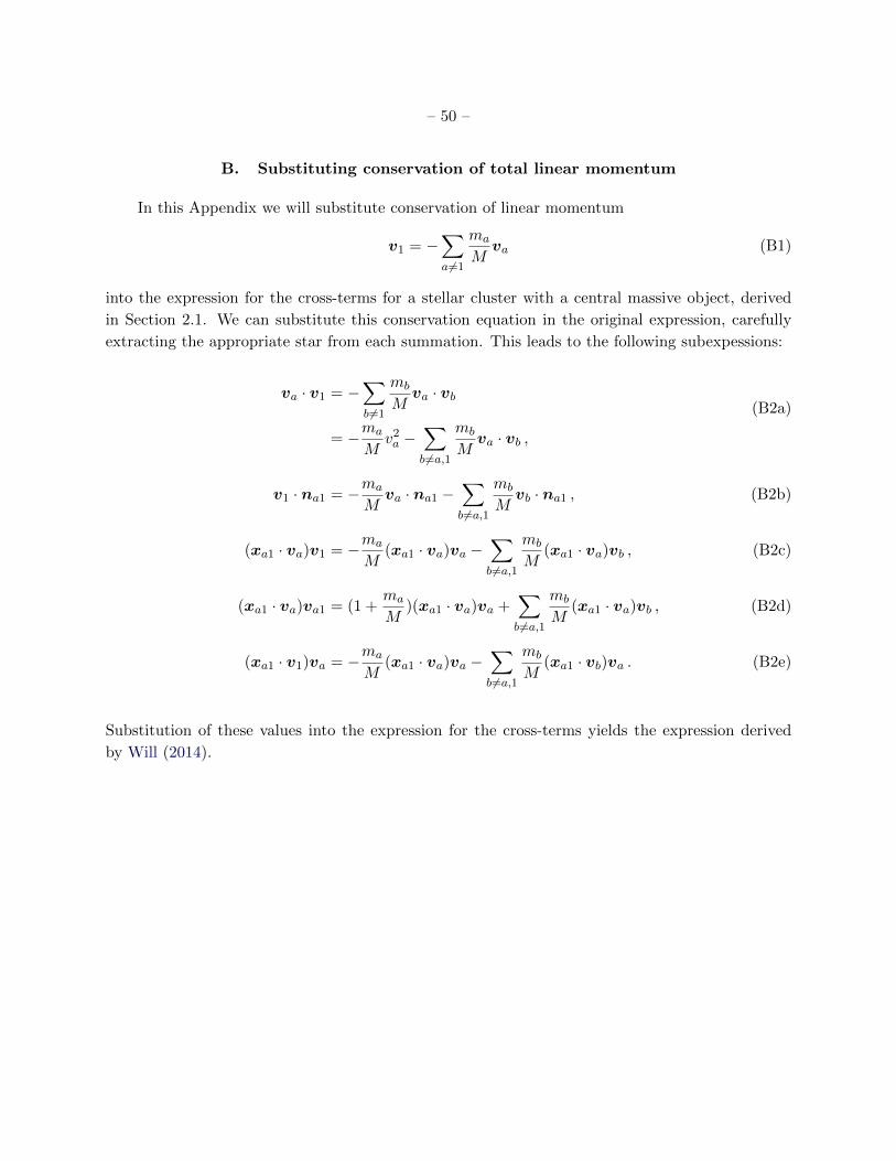
– 50 –
B. Substituting conservation of total linear momentum
In this Appendix we will substitute conservation of linear momentum
v1 = −∑a6=1
ma
Mva (B1)
into the expression for the cross-terms for a stellar cluster with a central massive object, derived
in Section 2.1. We can substitute this conservation equation in the original expression, carefully
extracting the appropriate star from each summation. This leads to the following subexpessions:
(B2a)va · v1 = −
∑b 6=1
mb
Mva · vb
= −ma
Mv2a −
∑b 6=a,1
mb
Mva · vb ,
(B2b)v1 · na1 = −ma
Mva · na1 −
∑b 6=a,1
mb
Mvb · na1 ,
(B2c)(xa1 · va)v1 = −ma
M(xa1 · va)va −
∑b6=a,1
mb
M(xa1 · va)vb ,
(B2d)(xa1 · va)va1 = (1 +ma
M)(xa1 · va)va +
∑b 6=a,1
mb
M(xa1 · va)vb ,
(B2e)(xa1 · v1)va = −ma
M(xa1 · va)va −
∑b6=a,1
mb
M(xa1 · vb)va .
Substitution of these values into the expression for the cross-terms yields the expression derived
by Will (2014).


![Post-Newtonian and Post-Minkowskian Two-Body Potentials ... lytic post-Newtonian (PN) models resummed within the e ective-one-body pre-scription [11;12]. They are respectively e cient](https://img.dokumen.tips/doc/110x75/5f0d067d7e708231d4384e69/post-newtonian-and-post-minkowskian-two-body-potentials-lytic-post-newtonian.jpg)