Embed Size (px)
Citation preview
NASA/CR-2000-210553
ICASE Report No. 2000-41
Possible Statistics of Two Coupled Random Fields:
Application to Passive Scalar
B. Dubrulle
CNRS, Toulouse, France
Guowei He
ICASE, Hampton, Virginia
November 2000

The NASA STI Program Office... in Profile
Since its founding, NASA has been dedicated
to the advancement of aeronautics and spacescience. The NASA Scientific and Technical
Information (STI) Program Office plays a key
part in helping NASA maintain this
important role.
The NASA STI Program Office is operated by
Langley Research Center, the lead center forNASA's scientific and technical information.
The NASA STI Program Office provides
access to the NASA STI Database, the
largest collection of aeronautical and space
science STI in the world. The Program Officeis also NASA's institutional mechanism for
disseminating the results of its research and
development activities. These results are
published by NASA in the NASA STI Report
Series, which includes the following report
types:
TECHNICAL PUBLICATION. Reports of
completed research or a major significant
phase of research that present the results
of NASA programs and include extensive
data or theoretical analysis. Includes
compilations of significant scientific andtechnical data and information deemed
to be of continuing reference value. NASA's
counterpart of peer-reviewed formal
professional papers, but having less
stringent limitations on manuscript
length and extent of graphic
presentations.
TECHNICAL MEMORANDUM.
Scientific and technical findings that are
preliminary or of specialized interest,
e.g., quick release reports, working
papers, and bibliographies that containminimal annotation. Does not contain
extensive analysis.
CONTRACTOR REPORT. Scientific and
technical findings by NASA-sponsored
contractors and grantees.
CONFERENCE PUBLICATIONS.
Collected papers from scientific and
technical conferences, symposia,
seminars, or other meetings sponsored or
cosponsored by NASA.
SPECIAL PUBLICATION. Scientific,
technical, or historical information from
NASA programs, projects, and missions,
often concerned with subjects having
substantial public interest.
TECHNICAL TRANSLATION. English-
language translations of foreign scientific
and technical material pertinent toNASA's mission.
Specialized services that complement the
STI Program Office's diverse offerings include
creating custom thesauri, building customized
data bases, organizing and publishing
research results.., even providing videos.
For more information about the NASA STI
Program Office, see the following:
• Access the NASA STI Program Home
Page at http://www.sti.nasa.gov
• Email your question via the Internet to
help@ sti.nasa.gov
• Fax your question to the NASA STI
Help Desk at (301) 621-0134
• Telephone the NASA STI Help Desk at
(301) 621-0390
Write to:
NASA STI Help Desk
NASA Center for AeroSpace Information7121 Standard Drive
Hanover, MD 21076-1320

NASA/CR-2000-210553
ICASE Report No. 2000-41
_i_:_ _ .:i_i!i....... _/_
Possible Statistics of Two Coupled Random Fields:
Application to Passive Scalar
B. Dubrulle
CNRS, Toulouse, France
Guowei He
ICASE, Hampton, Virginia
ICASE
NASA Langley Research Center
Hampton, Virginia
Operated by Universities Space Research Association
National Aeronautics andSpace Administration
Langley Research CenterHampton, Virginia 23681-2199
Prepared for Langley Research Centerunder Contract NAS 1-97046
November 2000

Available fi'om tile following:
NASA Center for AeroSpace hffomlation (CASI)
7121 Standard Drive
Hanover, MD 21076 1320
(301) 621 0390
National TectHficalhffomlation Service(NTIS)
5285 Port Royal Road
Spfingfield, VA22161 2171
(703) 487 4650

POSSIBLE STATISTICS OF TWO COUPLED RANDOM FIELDS:
APPLICATION TO PASSIVE SCALAR
B. DUBRULLE* AND GUOWEI HEt
Abstract. We use the relativity postulate of scale invariance to derive the similarity transformations
between two coupled scale-invariant random fields at different scales. We find the equations leading to
the scaling exponents. This formulation is applied to the case of passive scalars advected i) by a random
Gaussian velocity field; and ii) by a turbulent velocity field. In the Gaussian case, we show that the passive
scalar increments follow a log-Levy distribution generalizing Kraichnan's solution and, in an appropriate
limit, a log-normal distribution. In the turbulent case, we show that when the velocity increments follow
a log-Poisson statistics, the passive scalar increments follow a statistics close to log-Poisson. This result
explains the experimental observations of Ruiz et al. about the temperature increments.
Key words, scale invariance, scale transformation, scaling, turbulent scalar field
Subject classification. Fluid Mechanics
1. Introduction. Scale invariance [1] usually refers to physical fields keeping the same properties at
different scales. Therefore, scale invariance is often associated with the existence of power scaling laws. In
this case, the central characteristic quantities of the system are the scaling exponents. When a random field
is statistically scale invariant, each of its structure functions follows a power law, and there is a whole family
of exponents associated with its statistics.
To understand the underlying properties associated with the scaling exponents one can follow two paths:
first, try to measure or compute the scaling exponents with as high a precision as possible. This is the path
usually followed in critical phenomena, where scaling exponents are few, and appear to be universal, due to
some underlying conformal symmetry [2]. In turbulence, this path seems more difficult to follow, because the
number of scaling exponents to measure or compute, in order to know the statistics of the field, is infinite.
Therefore, parallel to the measurement or actual computation path, there seem to be the necessity of a more
formal path, devoted to understand link between the various scaling exponents. That way, the measure
or computation of only a few scaling exponents would hopefully enable the unraveling of the statistical
nature of the system. A natural way to establish link between scaling exponents is to use the symmetry
responsible for the existence of the scaling exponents, namely the scale invariance. This was the basis of
conformal theory [2] or multifractal theory [3]. More recently, Dubrulle et al. [1, 4, 5, 6] found that new
constraints on scaling exponents stemming from scale invariance could be found via an analogy between
scale invariance and relativistic dynamics inspired by a theory of Nottale [7] and of Pocheau [8]. This can
be used to classify the possible forms of scaling exponents according to the fixed points of the similarity
transformation. However, these results were restricted to one random scale invariant field (1D case). In
many physical situations, the dynamics involves at least two coupled random fields, such as transports of
passive scalars (coupling of velocity and scalar), magnetohydrodynamics (coupling of velocity and magnetic
*CNRS, URA 285, Observatoire, Midi-Pyr6n6es, 14 avenue Belin, F-31400 Toulouse, France (email:
[email protected])tICASE, Mail Stop 132C, NASA Langley Research Center, Hampton, VA 23681-0001 (email:[email protected]). This research
was supported by the National Aeronautics and Space Administration under NASA Contract No. NAS1-97046 while the author
was in residence at ICASE, NASA Langley Research Center, Hampton, VA 23681.
field)andturbulence(couplingoftransverseandlongitudinalvelocityincrements).Thegoalofthepresentpaperis thereforeto extendsomeoftheseresultsto thecaseoftwocoupledscaleinvariantrandomfields(2Dcase)andusethe2Dresultsto explorescalingof passivescalars.
Thetransportof passivescalars,for examplethetemperature0, is governed by the diffusion equation:
(1.1) 0t0 + (u. V)0 = aA0,
where the solenoidal velocity field u is either taken to be random or governed by the Navier-Stokes equation,
is molecular diffusivity. We are interested in scaling of passive scalar structure functions for given scaling
of velocity structure functions:
= + -
(1.2) S,_(e) = ((u(x + e) - u(x))n) ec e¢(n),
where ¢(n) and _(n) are the scaling exponents of velocity structure functions and scalar structure functions
respectively. We will use 2D similarity transformations to derive these possible scaling exponents.
This paper is organized as follows. After useful preliminaries regarding scale invariance (Section 2), the
2D similarity transformation of scale invariant fields is presented in Section 3. The results are applied to the
case of the transport of a passive scalar by a Gaussian velocity field in section 4 and by a turbulent velocity
field in section 5. We conclude the paper in section 6.
2. Preliminaries on scale invarlance. Scale invariance is a commonly used concept but sometimes,
rigorous definitions are lacking. In this section, we give a brief review on the rigorous definition of scale
dilation (or contraction), global and local scale invariance. Then, we discuss the existence of similarity
transformation between measurements of physical fields at different scales due to scale invariance.
Let (_(x), _ (x)) be a two-dimensional positive homogeneous random field [9] and dependent on scale
_. We define a family of scale dilation Sh,h' (A) via:
(2.1) Sh,h'(A) : _ --+ A_, _,¢_ --+ Ah_,Ah'¢_.
A two dimensional homogeneous random field is said to be globally scale invariant or, simply, scale invariant,
if (_(x), ¢f(x) ) and Sh, h, (,_)(_(X), el(X)) have the same statistical properties.
In log-variables, T = ln_, X = ln(_t), Y = ln(¢t), the globally scale invariance amounts to a transla-
tional invariance. This invariance is connected with the possibility to multiply any characteristic quantity
by an arbitrary constant, i.e. with the possibility to perform arbitrary changes of units in the system [1]. It
is a global scale invariance that leads to the existence of power laws of the moments of random homogeneous
fields:
(2.2) (¢?)
Scale invariance can be also considered as local [8]. Local scale invariance is connected with the invariance
of the system with respect to resolution changes. Indeed, consider a discrete slicing of the scale space _ _< L
in the form:
_i =, i_0, L = , N_0,
(2.3) _i = Ai_o, _i = Ai_o,

where,,(orequivalentlyN) and A characterize the resolution of the observations. _o0 and _0 are the units of
the observations. By local scale invariance, we require that the physical properties of the system be invariant
under changes of resolution, i.e. under changes of N. In fact, changes of N can be achieved by dilation of
,: , --+, _, which transform i into ia. It is also a transformation which transforms fJfj into (fJfj)_, and
_9i1_9 j into (_9i1_9j) a . Therefore:
A local scale dilation can be seen as a transformation for arbitrary a:
(2.4) f/f0 -+ ¢/¢0 -+ (¢/¢0)
A two dimensional homogeneous random field is said to be locally scale invariant if the physical fields
(_o_(x), %De(x)) are statistically in variant under local scale dilation.
Local scale invariance can be also seen as a change of rationalized unit system because it amounts to
multiply f0, _o0 and _0 by f0(f/f0) 1-_, _o0(_oAo0) 1-_ and _0(_/_0) 1-_. Therefore, global scale invariance
implies local scale invariance.
When the field (_oe(x), ¢e (x)) is globally scale invariant, all these changes of units can be characterized
by only one number: the exponent of their power law. This number labels the system of units and varies with
it. It is not an absolute quantity. All these remarks have been so far considered as rather obvious because
they do not lead to any specially useful information when applied to deterministic fields. For random fields,
however, < ¢_ > and < ¢_ > can be very different, and the application of our remarks can lead to very
interesting consequences about the exponents. In fact, they are not necessary additive anymore and can
obey more complicated composition law, which can be determined only from the requirement of local scale
invariance, as was shown in [6]. We now define the formalism which can be used to derive these composition
laws in the case of two coupled fields. This is done by a natural generalization of [1, 6] which we refer to for
more details.
3. Formalism and derivation of the composition laws.
3.1. Formalism. As noted previously, scale invariance amounts to a translational invariance when
logarithm of scale and fields are considered. We also would like to introduce a field variable which is
deterministic but keeps track of the possible different realizations of the process. A good way to reconcile
these two requirements is to introduce the log-variables [6]:
T - ln(flf°) - log K(f/f0),ln(SO
xn = (ln(¢U¢o) (¢U¢o)n )((¢U¢o)D
(3.1) yp = (ln(Ib_/Ib0) (¢_1¢o) p )
where K is the basis of the logarithm, f0 is an arbitrary length unit, ¢0, Ib0 two arbitrary field units (pos-
sibly random and/or scale dependent [1]), and n and p are real numbers. We note that ln(K), p and n
labels the system of subunits used to measure the length and fields. Then, globally scale invariance implies
homogeneity in these log-coordinates. Local scale invariance implies the existence of a group transformation
connecting different measures of the field at different scales. Formally, this means that we can find a simi-
larity transformation between (log K (fifo), Xn, Yp) and (log K, (fifo), Xn,, Yp, ). Since f is deterministic, it is

equivalentto change/(or_to changeT = lnK(_), so we can as well fix/( e.g. /( = e and let _ vary. The
transformation is now between (T = ln(_/_0), Xn, Yp) and (T' = ln(_'/_), Xn,, Yp,). We call it the similarity
transformation.
The derivatives U(n) = dXn/dT, V(p) = dYp/dT are analogous to the relative velocities. In our formal-
ism, they are just the local multifractal exponents [6].
3.2. Two-dlmenslonal similarity transformation. The possible similarity transformation can be
derived provided the system is both globally and locally scale invariant. Global scale invariance implies
that the transformation are linear [1]. Since nothing forbids a coupling between fields and scales, their most
general representation is a 3 × 3 matrix coupling X, Y and T. By local scale invariance, the set of such
3 × 3 matrices must form a (at least semi) group, depending on two parameters U and V [1]. Without loss
of generality, they may be written as:
(3.2) D E
GU HV
where A, B, D, E, G, H, U, V and , are some unknown functions of U and V to be determined. According
to the transformation (3.2), a field characterized by X = Y = 0 for any T in one reference field R = (n,p)
is transformed into X t = UT t, yt = VT t in another reference field R t = (nt,pt). This shows that (U, V) are
characteristic numbers labeling the change from (n,p) to (nt,pt). It is then natural to adopt U and V as the
group parameters.
To completely determine A, ...,, as a function of (U, V), an additional assumption is needed. From
physical considerations, we choose to postulate that the group of similarity transformations is commutative.
This means that it is equivalent to perform a transformation at scale f then ft or ft then f. This property is
generic in the group of scale dilation $_,(h, ht), at any given h and h t, which motivates our choice. Moreover,
it is a natural extension of the commutativity property in 1D [1]. Note that in such case, the commutativity
is guaranteed by the 1D Lie group structure and need not be postulated. Note also that in special relativity,
the third additional postulate is isotropy. This leads to a representation in term of rotations, which is NOT
commutative in D > 1. There is therefore no hope to find the Lorentz group as a special case of our similarity
transformations, contrary to the 1D case.
With this additional postulate, the form of the matrix (3.2) can be completely specified. The proof is
given in Appendix A. It is:
(3.3)
A = (1 - aU- jV),
D = -c(jU + dV),G == -h,
B = -(jU + dr),E = (1 - cdU - bV),
H = -k,
where, is a function of U and V obeying the transformation rule:
(3.4) ,(U",V") = ,( U', V'),( U, V)(1 - hUU' - kVV'),
with U tt, Ut,... V following (3.7). We were not able to find the exact expression of, in the general case,
but in the simple cases we study in the next two sections (where h = k = 0), , = 1 is always a solution. In
general, we postulate that , is a quadratic form in U and V, but the explicit value of the coefficient is not
needed in the derivation of the composition law.

Thecoemcientsa, b, c, d, h, k and j are parameters depending on the physical model. They satisfy
(3.5) h = ck, - k + ad + jb = j2 + d2 c
They are real if the scale symmetry is continuous [1].
Composing two transformations from reference fields R = (n,p) to R' = (n',p') and from R' = (n',p')
to R" = (n",p"), we obtain:
(3.6) (URIR", VRIR") = (URIR', VRIR') ® (UR'IR", VR'IR")
where ® is the composition law:
I U" = U+U'-aUU'-dVV'-j(U'V+UV')
1 - hUU' - kVV'
(3.7) V" = V + V'-cjUU'-bVV'-cd(U'V +UV')1 - hUU I - kVV I
Like in 1D, the composition law can be characterized by its fixed points, which depend on the parameters
a, b, c, d, h, k,j. It can also be used to determine the scaling exponents, by an appropriate choice of R, R'
and R". In both cases, the general computation is rather cumbersome and complicated by the large number
of degenerate situations (collapsing or vanishing fixed points). We treat in the following sections two special
cases where the computations are tractable. We emphasize that the case c = 0 implies no influence of X
over Y and is relevant to the case of the passive scalar dynamics when X is taken as the passive scalar
log-coordinate and Y as the velocity field log-coordinate.
3.3. The choice of the reference field. To obtain the composition law for the scaling exponents, we
must make precise the link between X, Y and U, V. This depends on the choice of ¢0 and _0. As emphasized
in [1], a convenient choice is to take ¢0 =< ln(¢_) > and _0 =< ln(_) >. Physically, these quantities are
the most probable values of the fields ¢ and ¢. The log coordinate X and Y then characterize deviations
with respect to these most probable values, and are a measure of the intermittency of the fields. In such
simple case, it is easy to check [6] that the scaling exponents for ¢ and ¢ are simply connected to X and Y,
via:
dXnOn_(n) - 0n_(n)ln=0 -- dT '
(3.8) Opt(p) - Op_(p)lp=O -- dT "
Now, the connection between U, V and _(n), _(p) can be made more clearly by exploiting the remark
made in Section III.A. Indeed, considering the transformation from X = 0, Y = 0 to Xn = (0_(n) -
0n_(n)l_=0)T,_ p = (0pC(p) - O_¢(p)l_=o)T, we get:
dXnU(n) = 0_(n) - 0_(n)[n=0 - dT '
(3.9) V(p) = Opt(p) - Op_(p)lp=O - dT "
This shows the existence of a bijection between (U, V) and (n,p). It unambiguously defines an internal
composition law _ on (n,p), through a transport of the group structure ®:
(U, V)((n,p)_(n',p') = (U, V)(n,p)®(U, V)(n',p'),
(n,p)_(n',p') = (U -1, V-1)((U, V)(n,p)
(3.10) ®(U,V)(n',p')).

Fromthisproperty,wecandeducethattheshapeof 6 is thesameas(3.7),withdifferentparameters,characterizingthefixedpointsin the(n,p)space1.Wehave(n",p") = (n,p)6(n',p') with:
I n" = n+n'-c_nn'-Spp'-7(n'p+np')(3.11) 1 - unn' - XPP' '
p, = p + p' - vTnn' - ppp' - vS(n' p + np')1 - _nn' - XPP'
where the parameters a, p, 7, 5, 7, v, X characterize the fixed points of 6 and satisfy:
(3.12) _ = TX, - X + a5 + 7P = 72 + 52T
3.4. Computation of the scaling exponents. The correspondence established through eq. (3.10)
enables to classify the statistics of scale invariant random process, i.e., of the possible shapes for _(n), _(p),
on universal grounds. Consider eq. (3.10) with (n,p) = (n',p') = (1, 1). This provides a recursive equation
which allows the computation of (U, V) for any integer rn, and then, by continuation, on any real number,
namely:
E(m) -- (1, 1)6(1, 1)6...6(1, 1) -- (1, 1) _'q,
(U, V)(E(m)) = (U(1), V(1))®...®(U(1), V(1))
(3.13) = (U(1), V(1)) ['_].
Here the notation [rn] (resp. irn]), stands for the rn th iterate via ® (resp. 6): we have introduced the
notation E(rn) = (El (rn), E2(rn)) to generalize the exponentiation rn to real, defined by using infinitesimal
n and p. It is now technically possible to calculate the values of the _(n) and _(p). The set of equations
(3.7, 3.10, 3.11, 3.13) is a mathematically well-posed problem. Indeed, inverting (3.8), we get:
d_(n) _ d_(n) In=0 + U(1) ['i-l(n)]dn dn
(3.14) d_(n) _ d_(n)I_=0 + V(1) [E_I(_)].dn dn
This provides a symbolic representation of the possible shape for the scaling exponents, depending on the
fixed points of the composition law. As an example, we treat below some tractable examples, where the
fixed points are simple. Since we are interested in the case where no coupling exist from the field 0 onto
(passive scalar limit), we see that this imposes c = v = 0. These values are adopted from now on.
4. Passive scalar advected by a Gaussian field. We consider here the case where u is a Gaussian
velocity field, with 2n-th order structure functions scaling like:
(4.1) <(Su_) 2_} - <(u(x + _)- u(x)) 2} _ _¢(2_).
Because u is Gaussian, it follows the simple "normal" scaling property:
(4.2) _(2n) = n_(2).
We are interested in the scaling properties of a passive scalar, advected by such a velocity field. Specifically,
we are looking for the scaling exponents _(2n) of the 2n th order structure function of temperature increments
defined as:
(4.3) < (8(x + _) - 8(x)) 2n >,._ _(2n).
1physically, these fixed points correspond to the limit beyond which the moments of the distribution in ¢ or _ are divergent,
see [6].

In theKraichnanmodel[10]oftheeq.(1.1)whereu is deltacorrelatedin time,a numberof exactresultshavebeenrecentlyestablished.Kraichnan[10]andGawedzkiandKupianen[11]haveshownthesecondorderscalingexponent_(2)is relatedto theexponent4(2)of thesecondorderstructurefunctionof thevelocityfieldby:
(4.4) _(2)=2 - 4(2).
Forscalingexponentsof higherorderstructurefunctions,bothperturbativeandnon-perturbativeresultsareavailable.In the limit where4(2)--+0, it wasshownbyBernardet al. [12]thatthescalingexponentsfollowthe "anomalous"law:
2n(n - 1)(4.5) _(2n) = n_(2) D + 2 _(2), 4(2) -+ 0,
where D is the space dimension. In the limit where 4(2) --+ 2, it was shown by [13, 14] that the anomalous
correction vanish, so that:
(4.6) _(2n)=n_(2), 4(2)--+2.
Chertkov et al. [15] used an expansion in the inverse 1/D of the space dimensionality to obtain:
(4.7) _(2n) = n_(2) 2n(_D- 1)4(2) , D -1 -+ 0,
which is consistent with the result (4.5) obtained by Bernard et al. [12].
On the other hand, Kraichnan [10] used the linear ansatz for the molecular-diffusion term and found a
non-perturbative result:
1v/4nD_(2) + (D - _(2)) 2 - _(D - _(2)).(4.8) _(2n) =
Note that this result is inconsistent with the 4(2) expansion of Bernard et a/[12]: using (4.4), one finds that
in the limit 4(2) --+ 0, the exponents _(2n) - n_(2) given by (4.8) tend to a finite limit which contradicts
(4.5).
We finally mention the exact non-perturbative calculation of the anomalous correction to fourth scaling
exponent P4 -- 2_(2) - _(4) obtained by Benzi et al. [16] in the case of a random shell-model for passive
scalar. This discrete toy model mimics most of the properties of the equation (1.1) [17]. In such model, the
properties of the scaling exponent are independent of ultraviolet and infrared boundary conditions, except
in the case where _(2) --+ 0 if the diffusive scale is kept fixed. In this last case, diffusive effects destroy the
inertial range scaling, and P4 _ 0, like in the models of [12] or [15], in the limit 4(2) --+ 2. Chertkov et al
also shows P4 -- 4(2 - 4(2))/D [18].
4.1. The scaling exponents. Let us now examine those predictions within the framework of the scale
invariant theory obtained in Section 3. In the stationary situation and in the non-diffusive limit, the equation
(1.1) is invariant under the transformation Sh,h' (A). This shows that, for the range of scale in which the
non-diffusive limit is meaningful (the so-called inertial range), the structure functions obey power laws (4.3),
where the scaling exponents _(n) may be a priori computed by using scale invariant theory.
In the Gaussian case, all the moments are convergent. The convergence of all moments implies that
the nonzero fixed points of the composition law for p must be -cx_ or cx_. That is possible only if _- -- U --
X = P = 0. Since the scaling exponent of the Gaussian field is linear, that is _(2n) = n_(2), V(n) has to
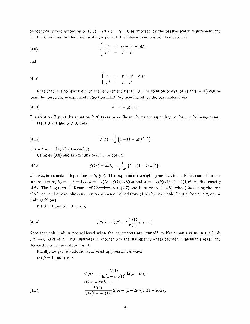
beidenticallyzeroaccordingto (3.8).With c -- h -- 0 as imposed by the passive scalar requirement and
b = k = 0 required by the linear scaling exponent, the relevant composition law becomes:
U" = U+U'-aUU'(4.9) V" = V+V'
and
n tt : n "-_ n t -- oznn t(4.10) P" = P+P'
Note that it is compatible with the requirement V(p) = 0. The solution of eqs. (4.9) and (4.10) can be
found by iteration, as explained in Section III.D. We now introduce the parameter/3 via
(4.11) /3 = 1 - aU(1).
The solution U(p) of the equation (4.9) takes two different forms corresponding to the two following cases:
(1) If/3 # 1 and a # 0, then
(4.12) U(n) = 1 ,(1- (1-owt) )_-11\a \ /
where A - 1 = in/3/ln(1 -an(l)).
Using eq.(3.8) and integrating over n, we obtain:
1 (1-(1-2an)X),(4.13) _(2n) = 2nho a_a
where h0 is a constant depending on 0n_(0). This expression is a slight generalization of Kraichnan's formula.
Indeed, setting h0 = 0, A = 1/2, a = -2(D - _(2))/D_(2) and a = -2D_(2)/(D - _(2)) 2, we find exactly
(4.8). The "log-normal" formula of Chertkov et al (4.7) and Bernard et al (4.5), with _(2n) being the sum
of a linear and a parabolic contribution is then obtained from (4.13) by taking the limit either A --+ 2, or the
limit as follows.
(2) /3 = 1 and a = 0. Then,
(4.14) _(2n) - n_(2) = 2_n(n - 1).
Note that this limit is not achieved when the parameters are "tuned" to Kraichnan's value in the limit
¢(2) --+ 0, _(2) --+ 2. This illustrates in another way the discrepancy arises between Kraichnan's result and
Bernard et al.'s asymptotic result.
Finally, we get two additional interesting possibilities when
(3) /3=landa#0
(4.15)
U(n) = U(1) ln(1 - an),ln(1 - an(l))
_(2n) = 2nho +
U(1) [2an - (1 - 2an)ln(1 - 2an)].aln(1 - an(l))

This expression tends towards the log-normal asymptotic form when c_ --+ 0.
(4) fl_landc¢=O
U(n) =1_ (1 _ fin�n(1))a
n(1) (1- fl2n/n(1))(4.16) _(2n) = 2nho + _ .
This is the log-Poisson law [19, 20, 21], which again tends to a log-normal in the limit fl --+ 1.
4.2. Discussion. Our result obviously generalizes the results of [10, 12, 15], using four arbitrary con-
stants. Because we use symmetry arguments, we cannot obtain any quantitative information about the
value of the anomalous correction. Only "matching" with exact computations (starting from the original
equations) can provide values for these constants. In the present case, we have four arbitrary parameters: a,
U(1), a and h0. These parameters can be arbitrary function of 4(2) which need to be determined. The exact
result (4.4) enables to write an equation linking our four parameters to 4(2). Besides that, the asymptotic
expressions of Bernard et al. and Chertkov et a/. only provide asymptotic expressions for U(1), and the
condition that a must tend to zero as D --+ oc or 4(2) --+ 0. This obviously does not constrain our parameters
enough, so we shall not bother to try to exhibit one out of the many solutions which fits all the requirement.
It would be interesting, as one gets more and more precise numerical result as those obtained by Frisch et
a/. [22], to try to derive the four parameters for any given value of 4(2), and see if they are enough to fit the
whole collection of exponents at this value of 4(2). This would provide a test of the present theory.
5. Passive scalar advected by turbulent flow. In this Section, we consider the case where the
velocity field u follows the Navier-Stokes equations:
VP(5.1) cgtu + (u. V)u - + pAv + f.
P
Here p is fluid density, f force, P pressure and p viscosity. Eq. (1.1) indicates that the passive scalar is
transported by the turbulence. Eq. (5.1) shows that the dynamics of the velocity field is not influenced by
the passive scalars.
In the stationary unforced inviscid limit (p, _ --+ 0), the set of equations (1.1,5.1) is invariant under
the transformation Sh,h' (A). This shows that for the range of scale in which the inviscid unforced limit is
meaningful (the so-called inertial range) the structure functions of velocity and passive scalar obey power
laws (1.2). Dimensional considerations lead to the prediction _(n) = _(n) = n/3. However, the experiments
and numerical simulations do not support the predictions. These exponents are observed to deviate from
the linear laws and the deviation is higher for the temperature than for the velocity. It is believed that the
deviations are due to intermittency of velocity and scalar dissipations.
Many models have been proposed to reproduce the scaling exponents of velocity structures. Among
them, She and Leveque's model [19] gives an excellent prediction of experimental results without any free
parameters. Later, this model is shown to be equivalent to assume that velocity increments follow a log-
Poisson statistics [20, 23]. The log-Poisson statistics converges to a log-normal statistics under a suitable
limit. In fact, a recent careful analysis [24] of turbulent data using wavelet transform indicated that the
turbulence is so close to log-normal that distinguishing between log-Poisson and log-normal statistics is
impossible, given the available amount of turbulent data. Therefore, we shall assume in the following
discussion that the turbulent velocity is log-Poisson, and then take the suitable limit towards log-normal
statistics to examine whether the passive scalar statistics can help in making the distinction.

Asanextensionof log-Poissonstatisticsofvelocityfields,CaoandChen[25]assumeda bivariablelog-Poissondistributionforjoint momentsof velocitydissipationc_andscalardissipationN_. This assumption
implies that passive scalars also obey log-Poisson statistics, which is in remarkable agreement with the results
of numerical simulations. Ruiz, Baudet and Ciliberto's recent experiments [26] also provide strong evidence
to support log-Poisson statistics of passive scalars. He et al. [21] propose a hierarchical relation for the joint
moments to explain why passive scalars must be log-Poisson. In the following, we explore the possibility of
log-Poisson statistics of passive scalars within the formalism developed in Section 3.
5.1. The scaling exponents. A remarkable simplification occurs from dynamical considerations: since
velocity dynamics is not influenced by the scalar dynamics, that is, the composition law for V must be
independent of U, one must choose c = h = _- = U = 0. Moreover, to select the log-Poisson statistics for
velocity increments [4] requires k = 0 and/3 = _ = 0. Therefore, the relevant composition law in this case is:
U" = U'+U-aU'U-dV'V-j[U'V+UV'](5.2) V" = V I + V - bWV
and
(5.3){ n tt = n t+n-(_n_n-_p_p-_/[n_p+np _]p, = pl + p
A rescaling of U and V by an arbitrary factor t, and of a, b, d and j by 1/t leaves (5.2) unchanged. At
the same time, a rescaling of n and p by l/t, and a rescaling of (_, 5, 7 by a factor t leaves (5.3) unchanged.
Since the scaling exponents depends only on the derivative of U and V with respect to n and p, we may
assume without loss of generality that, say, p(1) = 1.
The equation (5.2) has one stable fixed point
b-j 1(5.4) U+- ab ' V, =
and one unstable fixed point
1(5.5) u_- J v,=-.
ab ' b
We solve (5.2) and (5.3) and get an implicit representation of the solution via,
(5.6)
where
(5.7)
and
U[n(m)] = (U+ - U_)(1-/3_) + V,(1-/3_)V[p(m)] = V,(1-/3_)
U(1)/31 : 1
u+-u_V(1)
/32=1---V,
10

{ ( a2 ) 1-a_+ a2rn(5.8) n(rn) --- n(1) 1 - al 1 - al 1 - al
where
al -- 1 - an(l) - 7,
(5.9) a2 = -5 - 7n(1).
Here, n(1) is a free parameters. To avoid any discontinuity while ensuring n(0) = 0, we shall only assume
that n(0) tends to a2 when al tends to 0. Note here that the log-normal shape for the velocity increments
is obtained by letting/32 --+ 1, in which case the function U simply becomes:
(5.10) U(rn) = (U+ - U_) (1 -/3_) + rn.
To get U(n) as a closed form, one needs to invert the function n(m) given by (5.8). This is analytically
possible only for special values of the parameters, otherwise one can only use the implicit representation
(5.6) and (5.8). The special values where an explicit formulation of U(n) is possible are:
1) when a2 = 0: we get:
U(n) : (U+ - U_) (1 - (1 + n/a3) )'1-1)
+ V, (1 - (1 + n/a3)'x2-1),
V(p) = V, (1 -/3P),
_(n) : nh_ + a3(U+ - U_) (1 - (1 + n/a3) )'_),_1
+_-2V*a3 (1 - (1 + n/a3) "x2-1)
V,
(5.11) _(p) = ph¢ - ln/3_ (1 -/3P),
where Ai - 1 = ln/3J ln(al), for i = 1, 2, a3 = n(1)/(al - 1) and h f and he are integration constants. The
shape for _ is the usual log-Poisson shape. The shape for _ is a superposition of log-levy function. In the
log-normal limit for the velocity increments, one gets a different shape:
_(n) : nh_ + a3(U+ - U_) (1 - (1 +n/a3) )'_ ),_1
+ a3 ((1 + n/a3)ln(1 + n/a3) - n/a3),
p2(5.12) ¢(p) = ph¢ + _.
So the log-normal limit is not really simpler than the general solution.
2) when al : 0, we get:
U(rt) = (U+ -U_) (1- /31/n(1)) -'_- V, (1-- /32)n/n(1)) ,
V(p) = V, (1 -/3P),
n(1)(U+-U_) (1 _/31/n(1))= - ln-/31
n(1)V, (1 _/3_/n(1))in/32
V,
(5.13) ((p) = ph¢ - in/3_ (1 -/3P),
11

where he and h f are integration constants. In this case, they are scaling exponents connected with the
properties of the rarest events (the most intermittent structures), whose connexion with finite size effects is
discussed in [5]. The physical interpretation of the parameters appearing in (5.13) is obtained by taking the
limit n --+ oe or p --+ oe, when /_1 and/32 are less than one. We find that
_(n) _ nh_ - n(1)(U+ - U_ )/ ln/31 - n(1)V,/ ln _2
and
_(p) oc ph¢ - 17,/lnfl2.
This suggests interpreting -n(1)(U+ - U_)/lnfll - n(1)V,/lnfl2 and -V,/lnfl2 as the codimensions of
the most intermittent structures of the passive scalar and of the velocity. At this stage, we can make an
interesting remark: when n(1) is small (this is a case of weak coupling between passive scalar and velocity),
the last term in (5.13c) can be neglected. In this case, the scaling exponents of the passive scalar have a log-
Poisson shape. We show later by fitting the experimental data that this coupling coefficient is indeed small.
This therefore explains the observation in [26]. Also, we note that the scaling exponents (5.13) reassemble a
log-Poisson distribution with two "atoms", whose existence was conjectured in [23]. Finally, it is interesting
to consider the limit where the velocity increments are log-normal. In that case, we get:
n(1)(g+ - g_) V(1)n 2[ n __l__/_l/n(1))-F 2n(1)= - Vn- l --'
V(1)p 2(5.14) _(p) -- ph¢ + _,
In that case, the scaling exponents are the superposition of an exponential log-Poisson shape, and of a
parabolic log-normal shape. At large positive n (if /_1 < 1), the parabolic shape dominates the scaling
behavior, and one does not observe the simple linear asymptotics existing in the log-Poisson case. This
observation could be used as a tool to discriminate between log-Poisson and log-normal velocity increments,
by considering the statistics of passive scalars. This is an indirect check, but in some experimental settings,
this might actually prove easier than the direct check.
In all other cases, we may only obtain an implicit representation of the scaling exponent by using the
chain rule d_/drn = d_/dn . dn/drn.
5.2. Value of the constants. We obtained different explicit and implicit forms of scaling exponents
depending on several constants. In the most general (implicit) case, we have 9 free parameters. In the
simplest case (number 2), we have 6 free parameters. We need the same number of constraints to compute
these parameters. For he, /_1 and V,/ln_2, we can use the values obtained by [19], which provide a good
fit of the velocity increments: he = 1/9, /32 = 0.88 and V,/ln_2 = 2. For the remaining parameters,
we need to use values measured for the passive scalar. Given the available precision of the measures, it
is not really realistic to consider more than n = 5 or n = 6 scaling exponents for computing the values
of the constants. It is then only possible to determine the constants in the log-Poisson case, where only
three remaining parameters need to be determined. This simplification enables a partial determination
of the parameters. If the most intermittent structure have respectively vortex filaments and temperature
sheets, as observed in numerical simulations [27, 28], their codimensions are approximatively one and two.
By considering that the most intense energy dissipation events are only driven by the mean transfer term
(< ((_v) 3 >) and using the K62 refined similarity hypothesis [29], She and L6veque [19] obtain he = 1/9, and
12

2
1.5
0.5
0
'''1 .... I .... I ....
i t
.... I .... I .... I ....
2 4 6 8
n
FIG. 5.1. Comparison between the experimental data of Ruiz et al. (diamonds) and formula (49) with: A set of parameter
derived by physical arguments copying the argumentation of She and Leveque [19] for the velocity increments. This gives
(hs, fix, n(1), U+ - U-, he, V., f12) = (1/9, 0.985, 0.1, 0.015, 1/9, 0.26, 0.88) (dash line); A set of parameters derived by a best fit
to the data (hs, ill, n(1), U+ - U_, he, V., f12) = (0.06, 0.915, 0.25, 0.12, 1/9, 0.26, 0.88) (solid line).
then, using _(3) = 1,/_3 = 2/3. A same kind of argument also leads to h f = 1/9. Indeed, if we suppose that
the most intense temperature dissipation events are only driven by < (Sv) 3 > and < 5v(58) 2 >, we obtain
N _ _ O 2 < (5v)3 >1/3 / < 5v(50)2 >, where O is some constant temperature. Since < (Sv) 3 >_ _ and
< 5v(58) 2 >_ _, we obtain N _ _ _-2/3. Then, by using the refined Obukhov-Corrsin hypothesis ([30]), we
get h f = 1/9 + hN/2 + 1/3 = 1/9. We may then use these values and vary n(1) and/_1 to obtain the best fit
with the data. The result is given in Figure 1 for n(1) = 0.1 and /_1 ---- 0.86. It is not really good, especially
at large n where the formula gives a much larger value than the data. This is because the value h f = 1/9 is
too high. A three parameter fit of the data gives h f = 0.06, n(1) = 0.25,/_1 ---- 0.7, resulting in a codimension
of 0.84 for the passive scalar rarest events. The result is displayed in Figure 1.
Certainly, more work is needed to understand the meaning of the parameters. A recent work of Dubrulle
[5] [31] suggest that some of them might be linked with finite size effects. Work is in progress in that
direction.
6. Conclusion and discussion. In this paper, we develop a formalism leading to the equations fol-
lowed by the scaling exponents of two-dimensional scale invariant random fields. It is the extension of [1] on
one-dimensional random fields. We do not make any assumption on (statistical) relations of the two random
fields. For example, they may be independent of each other or anisotropic. Thus, the two random fields pos-
sess independent scaling exponents and they may have different limit velocities. This situation is completely
different from the relativity theory of motion, where the limit velocity is the same one (light velocity) in
each direction. We begin with the structures of transformation group, and then compute the transformation
matrix. The composition law, derived from the similarity transformation, indicates the equations relating
the different scaling exponents. Based on the scaling exponent equations, the classification of all exponents
is possible by the computation of the fixed points of the transformation. This is performed in a simple case,
the passive scalar advected by i) a random Gaussian velocity field; and ii) a turbulent velocity field.
13

In the Gaussian case, we show that the passive scalar increments follow a log-levy distribution gener-
alizing the solution of Kraichnan. This distribution tends in an appropriate asymptotic limit, towards a
log-normal distribution. The anomalous correction to the scaling exponent can be matched with the Kraich-
nan solution [10] or with recent perturbative expansions of Chertkov et al. [15] and Bernard et al. [12] via
an appropriate tuning of the parameters, which cannot be predicted by our simple symmetry arguments.
In the turbulent case, we show that when the velocity increments follow log-Poisson statistics, the passive
scalar increments follow various different statistics, the simplest one being close to log-Poisson. It is in fact a
log-Poisson distribution with two "atoms", thereby providing an explicit example of a random system with
more than one atom whose existence was conjectured in [23]. This result provides an explanation of the
experimental findings of [26] about the temperature increments.
We note that scale invariance may play a role in many other physical problems. It would then be
interesting to consider other values of the parameters to describe other physical situations such as scaling
laws in magneto-hydrodynamics.
Acknowledgments G. W. He expresses his gratitude to Lachieze-Rey for discussion around the relativity
of motion. He also would like to thank SAP for its hospitality. B. Dubrulle acknowledges useful discussions
with M. Vergassola.
Appendix A: Derivation of Similarity Transformations
We show that the similarity transformation compatible with the following postulates are the solution
(3.3) by generalizing the method [1] to the two-dimensional case:
Posulate 1. The log-coordinates are invariant under global translation.
Posulate 2: Among all imaginable reference fields, there exist a continuous class of equivalent reference
fields built on scale invariant fields.
Posulate 3: the group of similarity transformations is commutative.
Postulate 2 implies that the composition of two similarity transformations with respective parameters
(U, V) and (U I, W) should be a similarity transformation, associated to a third parameter noted (U", V").
Composition of two transformations in (3.2) then gives
(6.1)
the transformation (U, V).
(6.1.1) and (6.1.5) give
(6.2)
A" = AA' + BD' +, G'UU'
B" = AB I + BE I + , HIUW
,"U" = A,'U'+B,'V'+,, 'U
D" = DA' + ED' + , G'VU'
E II = DB I+EE I+,HIVW
,"V" -- D,'U'+E,'V'+,, 'V
G"U" = GA'U + HD'V +, G'U'
H"V" = GB'U + HE'V +, H'V'
," = G, 'UU' + H, 'VV' + ,, '
We now use the Postulate 3 about commutativity. We first apply the transformation (U I, W) and then
By comparison with (6.1), we obtain several equations. For example, equations
BDI - BID = UUI(, IG- , G'),
DBI - DIB = VVI(, IH-, H').
14
Factorizing(6.2)leadsto
(6.3) D = cB, G = -h, ,H = -k, ,
where c, h, k are adjustable parameters.
Substituting (6.3) into (6.1.2) and (6.1.4), and then comparing their coefficients, we obtain
h=ck.
The same technique applied to (6.1.3) and (6.1.6) gives
(6.4)
A = (1-aU-jV),
B = -(jU+dV),
E = (1-cdU-bV),
where a,b,d,j are adjustable parameters. (6.3) and (6.4) are solutions of equations (6.1) provided the
parameters follow
-k + ad + jb = j2 + dS c.
This completes our proof.
REFERENCES
[1] B. DUBRULLE AND F. GRANER, Possible statistics of invariant systems, J. Phys. II France, 6 (1996),
pp. 797-816.
[2] A. M. POLYAKOV, The theory of turbulence in 2-dimensions, Nucl. Phys., B396 (1993), pp. 367-385.
[3] G. PARISI AND W. FRISCH, Turbulence and Predictability in Geophysical Fluid Dynamics, Proceed.
Intern. School of Physics "E. Fermi", 1983, Varena, Italy, pp. 71-88, eds. M. Ghil, R. Benzi and G.
Parisi, North-Holland.
[4] B. DUBRULLE AND F. GRANER, Scale invariant and scaling exponents in fully developed turbulence, J.
Phys. II France, 6 (1996), pp. 817-824.
[5] B. DUBRULLE, Anomalous scaling and generic structure function in turbulence, J. Phys. II France, 6
(1996), pp. 1825-1840.
[6] B. DUBRULLE, F. BREON, F. GRANER, AND A. POCHEAU, Towards an universal classification of scale
invariant processes, European Phys. J. B., 4 (1998), pp. 89-99.
[7] L. NOTTALE, Fractal space-time and microphysics, World Scientific, Singapore, 1993.
[8] A. POCHEAU, Scale-invariance in turbulent front propagation, Phys. Rev. E, 49 (1994), pp. 1109-1122.
[9] See [1] for the possibility to deal with non-positive fields.
[10] R. H. KRAICHNAN, Anomalous scaling of a randomly advected passive scalar, Phys. Rev. Lett., 72
(1994), pp. 1016-1019.
[11] K. GAWEDZKI AND A. KUPIAINEN, Anomalous scaling of the passive scalar, Phys. Rev. Lett., 75 (1995),
pp. 3834-3837.
[12] D. BERNARD, K. GAWEDZKI, AND A. KUPIAINEN, Anomalous scaling in the N-point functions of a
passive scalar, Phys. Rev. E, 54 (1996), pp. 2564-2572.
15

[13]B. I. SHRAIMANANDE. D. SIGGIALagrangian path integrals and fluctuations in random flow, Phys.
Rev. E, 49 (1994), pp. 2912-291"/.
[14] M. CHERTKOV, G. FALKOVICH, I. KOLOKOLOV, AND V. LEBEDEV, Statistics of a passive scalar
advected by a large-scale 2-dimensional velocity-field: Analytical solution, Phys. Rev. E, 51 (1995),
pp. 5609-562"/.
[15] M. CHERTKOV, G. FALKOVICH, AND V. LEBEDEV, Nonuniversality of the scaling exponents of a passive
scalar convected by a random flow, Phys. Rev. Lett., "/6 (1996), pp. 3"/07-3710.
[16] R. BENZI, L. BIFERALE, AND A. WIRTH, Analytic calculation of anomalous scaling in random shell
models for a passive scalar, Phys. Rev. Lett., "/8 (1996), pp. 4926-4929.
[1"/] A. WIRTH AND L. BIFERALE, Anomalous scaling in random shell models for passive scalars, Phys. Rev.
E, 54 (1997), pp. 4982-4989.
[18] M. CHERTKOV, G. FALKOVICH, I. KOLOKOLOV, AND V. LEBEDEV, Normal and anomalous scaling of
the _th-order correlation-function of a randomly advected passive scalar, Phys. Rev. E, 52 (1995), pp.
4924-4941.
[19] Z. S. SHE AND E. LEVEQUE, Universal scaling laws in fully developed turbulence, Phys. Rev. Lett., "/2
(1994), pp. 336-339.
[20] B. DUBRULLE, Intermittency in fully-developed turbulence: Log-Poisson statistics and generalized scale
covariance, Phys. Rev. Lett., "/3 (1994), pp. 959-962.
[21] G. W. HE, S. CHEN, AND G. DOOLEN, Hierarchy of structure functions for passives scalars advected
by turbulent flows, Phys. Lett. A., 246 (1998), pp. 135-138.
[22] U. FRISCH, A. MAZZINO, AND M. VERGASSOLA, Intermittency in passive scalar advection, Phys. Rev.
Lett., 80 (1998), pp. 5532-5535.
[23] Z. S. SHE AND E. C. WAYMIRE, Quantized energy cascade and log-Poisson statistics in fully developed
turbulence, Phys. Rev. Lett., "/4 (1995), pp. 262-265.
[24] A. ARNEODO, S. MANEVILLE, AND J-F. MUZY, Towards log-normal statistics in high Reynolds number
turbulence, European Phys. J. B., 1 (1998), pp. 129-140.
[25] N. CAO AND S. CHEN, An intermittency model for passive-scalar turbulence, Phys. Fluids, 9 (1996),
pp. 1203-1205.
[26] G. RUIZ-CHAVARRIA, C. BAUDET, AND S. CILIBERTO, Scaling laws and dissipation scale of a passive
scalar in fully developed turbulence, Physica D, 99 (1996) pp. 369-380.
[2"/] A. VINCENT AND M. MENEGUZZI, The spatial structure and statistical properties of homogeneous tur-
bulence, J. Fluid Mech., 225 (1991), pp. 1-20; Z. S. SHE, E. JACKSON, AND S. ORSZAG, Intermittent
vortex structures in homogeneous isotropic turbulence, Nature, 344 (1990), pp. 226-228.
[28] A. PUMIR, Small-scale properties of scalar and velocity differences in 3-dimensional turbulence, Phys.
Fluids, 6 (1994), pp. 39"/4-3984.
[29] U. FRISCH, Turbulence: The legacy of A.N. Kolmogorov, Cambridge University Press, Cambridge, 1995.
[30] A. M. OBUKHOV, Structure of the temperature field in turbulent flows, Izv. Akad. Nauk SEER, Ser.
Geogr. Geofiz. 13 (1949) p. 58; S. CORRSIN, On the spectrum of isotropic temperature fluctuations in
isotropic turbulence, J. Appl. Phys., 22 (1951), p. 469.
[31] G. W. HE AND B. DUBRULLE, About generalized scaling for passive scalars in fully developed turbulence,
J. Phys. II France, 7 (199"/), pp. "/93-800.
16

Form Approved
REPORT DOCUMENTATION PAGE OMB No. 0704-0188
Public reporting burden for this collection of information is estimated to average 1 hour per response, including the time for reviewing instructions, searching existing data sources,gathering and maintaining the data needed, and completing and reviewing the collection of information. Send comments regarding this burden estimate or any other aspect of thiscollection of information, including suggestions for reducing this burden, to Washington Headquarters Services, Directorate for Information Operations and Reports, 1215 JeffersonDavis Highway, Suite 1204, Arlington, VA 22202-4302, and to the Office of Management and Budget, Paperwork Reduction Project (0704-0188), Washington, DC 20503.
1. AGENCY USE ONLY(Leave blank) 2. REPORT DATE 3. REPORT TYPE AND DATES COVERED
November 2000 Contractor Report
4. TITLE AND SUBTITLE 5. FUNDING NUMBERS
Possible statistics of two coupled random fields: Application to
passive scalar
6. AUTHOR(S)B. Dubrulle and Guowei He
7. PERFORMING ORGANIZATION NAME(S) AND ADDRESS(ES)ICASE
Mail Stop 132C
NASA Langley Research Center
Hampton, VA 23681-2199
9. SPONSORING/MONITORING AGENCY NAME(S) AND ADDRESS(ES)
National Aeronautics and Space Administration
Langley Research Center
Hampton, VA 23681-2199
C NAS1-97046
WU 505-90-52-01
8. PERFORMING ORGANIZATION
REPORT NUMBER
ICASE Report No. 2000-41
10. SPONSORING/MONITORINGAGENCY REPORT NUMBER
NASA/CR-2000-210553ICASE Report No. 2000-41
11. SUPPLEMENTARY NOTES
Langley Technical Monitor: Dennis M. BushnellFinal Report
Submitted to the European Journal of Physics C.
12a. DISTRIBUTION/AVAILABILITY STATEMENT
Unclassified-Unlimited
Subject Category 34Distribution: Nonstandard
Availability: NASA-CASI (301) 621-0390
12b. DISTRIBUTION CODE
13. ABSTRACT (Maximum 200 words)
We use the relativity postulate of scale invariance to derive the similarity transformations between two coupled scale-
invariant random fields at different scales. We find the equations leading to the scaling exponents. This formulation
is applied to the case of passive scalars advected i) by a random Gaussian velocity field; and ii) by a turbulent velocity
field. In the Gaussian case, we show that the passive scalar increments follow a log-Levy distribution generalizing
Kraichnan's solution and, in an appropriate limit, a log-normal distribution. In the turbulent case, we show thatwhen the velocity increments follow a log-Poisson statistics, the passive scalar increments follow a statistics close to
log-Poisson. This result explains the experimental observations of Ruiz et al. about the temperature increments.
14. SUBJECT TERMS
scale invariance, scale transformation, scaling, turbulent scalar field
17. SECURITY CLASSIFICATION
OF REPORT
Unclassified
NSN 7540-01-280-5500
18. SECURITY CLASSIFICATIOI_
OF THIS PAGE
Unclassified
15. NUMBER OF PAGES
21
16. PRICE CODE
A0319. SECURITY CLASSIFICATION 20. LIMITATION
OF ABSTRACT OF ABSTRACT
Standard Form 298(Rev. 2-89)Prescribed by ANSI Std. Z39-18298-102