Embed Size (px)
Citation preview

CER
N-T
HES
IS-2
016-
101
21/0
7/20
16
FACULDADE DE ENGENHARIA DA UNIVERSIDADE DO PORTO
POSITIONING SYSTEMS FOR
UNDERGROUND TUNNEL ENVIRONMENTS
Fernando Joaquim Leite Pereira
A dissertation submitted in partial fulfillment
of the requirements for the degree of
Doctor of Philosophy (PhD) in Telecommunications
Supervisor: Prof. Manuel Ricardo
Co-supervisor: Christian Theis
January, 2016

2
©Fernando Joaquim Leite Pereira 2016

POSITIONING SYSTEMS FOR
UNDERGROUND TUNNEL ENVIRONMENTS
Fernando Joaquim Leite Pereira
Examination committee:
President:
Doutor José Alfredo Ribeiro da Silva Matos
Examiners:
Doutor Nuno Manuel Ribeiro Preguiça
Doutor Jorge Miguel Sá Silva
Doutor Manuel Alberto Pereira Ricardo
Doutor Sérgio Reis Cunha
Thesis approved in public defense on 21 July 2016
__________________________________
(The supervisor - Prof. Manuel Ricardo)

4
The research work presented in this thesis has been performed within and funded by CERN,
Radiation Protection group, and acknowledges the collaboration of the IT/CO group at CERN,
the Wireless Networks (WiN) group at INESCTEC Porto and the initial financial support from
Fundação Ciência e Tecnologia (FCT) grant SFRH/BD/61791/2009.

i
ABSTRACT
In the last years the world has witnessed a remarkable change in the computing concept
by entering the mobile era. Incredibly powerful smartphones have proliferated at stunning pace
and tablet computers are capable of running demanding applications and meet new business
requirements. Being wireless, localization has become crucial not only to serve individuals but
also help companies in industrial and safety processes. In the context of the Radiation Protection
group at CERN, automatic localization, besides allowing to find people, would help improving the
radiation surveys performed regularly along the accelerator tunnels.
The research presented in this thesis attempts to answer questions relatively to the
viability of localization in a harsh conditions tunnel: “Is localization in a very long tunnel possible,
meeting its restrictions and without incurring prohibitive costs and infrastructure?”, “Can one
achieve meter-level accuracy with GSM deployed over leaky-feeder?”, “Is it possible to prototype
a localization system without a team of hardware engineers?”. To help answering those
questions, in the first place, a comprehensive characterization of the power profile in the LHC
tunnel was performed for both GSM and WLAN networks, which were transmitted over leaky-
feeder cable. Subsequently, several RSSI fingerprinting methods were explored. During the
characterization of the power profile, it was noticeable that GSM suffered low attenuation as it
propagated in the leaky feeder, at the same time it exhibited significant changes in a short scale
and among measurement sessions. Such findings motivated the research of new variants of KNN
better suited for leaky-feeder, as well as fusion techniques taking WLAN network in addition. It
was found that, even though KNN variants could bring interesting improvements, up to 27%,
much more significant gains were attained when considering signals from the WLAN as they
exhibited higher attenuation, enabling for 30 meters accuracy in 91% of the cases.
To further improve accuracy to the envisaged levels, time-of-flight techniques in
narrowband were investigated. A complementary positioning system based on phase delay and
aided by synchronization units is proposed and several tests are implemented using Software
Defined Radio. Despite the limitations of SDR in achieving phase stability, a method following a
round-trip design was shown to correctly stabilize and precisely detect small displacements.

ii
(This page was intentionally left blank)

iii
RESUMO
Nos últimos anos o mundo assistiu a uma profunda alteração da computação, com a
entrada na era mobile. Os smartphones têm proliferado rapidamente e cada vez mais os tablet
computers são capazes de correr aplicações exigentes, suportando novas atividades
empresariais. Sendo wireless, determinar a localização tornou-se, não só útil para pessoas
individuais, mas altamente importante em processos e segurança industriais. No grupo de
Radioprotecção do CERN, localização, além de permitir encontrar pessoas, poderá ajudar a
automatizar as atividades de levantamento dos níveis de radiação realizados regularmente nos
túneis dos aceleradores.
A investigação levada a cabo nesta tese procura responder a questões relacionadas com
a viabilidade de localização num túnel inóspito: “Será possível ter localização em túneis longos,
respeitando as suas restrições e sem incorrer custos e infraestruturas proibitivos?”, “Será possível
atingir acuidade na ordem de um metro com GSM propagado em leaky-feeder?”, “Poderemos
criar um protótipo de localização sem uma equipa de hardware?” Para responder a tais questões,
em primeiro lugar, procedeu-se à caracterização pormenorizada dos níveis de sinal GSM e WLAN
no túnel do LHC. Seguidamente vários métodos de localização, baseados em RSSI fingerprinting,
foram explorados. Durante a caraterização dos níveis de sinal verificou-se que a atenuação da
rede GSM, ao propagar no cabo, era reduzida e, adicionalmente, a potência do sinal variava
consideravelmente em pequena escala e entre as várias sessões de medida. Tal constatação
motivou a investigação de novas variantes do método KNN, melhor adaptadas a cabos radiantes
e que pudessem considerar vários sinais, especialmente WLAN. Os novos métodos conseguem
melhorias até 27% mas, no entanto, ganhos muito mais significativos de acuidade encontram-se
quando se considera WLAN, que revelando maior atenuação, chega a 30 metros em 91% casos.
Para se atingir os níveis de acuidade originalmente desejáveis, técnicas time-of-flight em
narrowband foram investigadas. É desenvolvido um sistema complementar de posicionamento
baseado em medidas de atraso de fase com unidades de sincronização, o qual é implementado
em Software-Defined-Radio. Não obstante a dificuldade do sistema estabilizar, um novo método
baseado em round-trip estabiliza e deteta pequenos deslocamentos com elevada precisão.

iv
(This page was intentionally left blank)
v
ACKNOWLEDGEMENTS
No words would be enough to thank all the people that directly or indirectly contributed
to this thesis. The whole PhD period had been fulfilled by experiences and people who marked
my life forever.
In the first place I would like to thank my supervisors Manuel Ricardo and Christian Theis,
who, somehow, deposited so much confidence in me and encouraged me to start, to strive to go
on and ultimately to finish this PhD work. Besides all the extraordinary technical support, the
motivation and perseverance they transmitted me were truly a decisive point. Moreover, they
would always be available to discuss, debate issues and help, which made the work possible even
under the most adverse scenarios. I also would like to direct a special acknowledge to profs.
Adriano Moreira and Sérgio Reis Cunha for their truly outstanding contribution to the thesis. Their
expert advice allowed the work to advance on major obstacles and greatly improved the scientific
value of the thesis and its publications.
I would like to thank my research fellows from INESC and CERN colleagues in general, for
the great work atmosphere and collaboration. I would dedicate a special thanks to Chris, Edi, Heli
and Mohammad, from whom I learned that friendship doesn’t have cultural borders. I must also
thank my lifelong friends Horacio, Ruben, Joaquim, Ivo for their support and presence in the best
and the most complicated moments, and couldn’t forget those I met in Geneva and with whom I
had the privilege to share much of my time: the geneva-gang members especially Dora, Rudi,
Daniel and Bruno.
A last very special word goes to my family, who I infinitely acknowledge for being a source
of inspiration and for their unconditional support in every moment. This work I dedicate to them.

vi
(This page was intentionally left blank)
vii
TABLE OF CONTENTS
CHAPTER 1 INTRODUCTION .............................................................................................................. 1
1.1 Context .......................................................................................................................... 1
1.2 Motivation .................................................................................................................... 2
1.2.1 CERN and the Large Hadron Collider (LHC) tunnels ................................................... 2
1.2.2 Radiation surveys at CERN ......................................................................................... 4
1.2.3 The Radiation Logging project ................................................................................... 5
1.3 Scope of the thesis ........................................................................................................ 7
1.3.1 Problem statement ..................................................................................................... 7
1.3.2 Proposed solution ....................................................................................................... 7
1.3.3 Original contributions ................................................................................................. 8
1.4 Thesis structure ............................................................................................................ 9
CHAPTER 2 WIRELESS LOCALIZATION FUNDAMENTALS ................................................................. 11
2.1 The “Wireless” channel .............................................................................................. 11
2.1.1 Radio Propagation ................................................................................................... 12
2.1.2 A shared medium for communications and localization ......................................... 14
2.2 Classification of Positioning systems .......................................................................... 16
2.2.1 Classification according to the topology ................................................................. 16
2.2.2 Classification according to user requirements ........................................................ 17
2.3 Wireless distance measurements .............................................................................. 19
2.3.1 Time-of-Flight .......................................................................................................... 20
2.3.2 Time-Difference-of-Arrival ....................................................................................... 22
2.3.3 Angle of Arrival ........................................................................................................ 24
2.3.4 Received Signal Strength Indicator (RSSI) ................................................................ 25
2.4 Position finding techniques ........................................................................................ 27
2.4.1 Proximity sensing ..................................................................................................... 27
2.4.2 Multilateration ........................................................................................................ 28
2.4.3 Dead-Reckoning ....................................................................................................... 32
2.5 Location fingerprinting techniques ............................................................................ 33
2.5.1 Deterministic location estimation ........................................................................... 34
2.5.2 Probabilistic location estimation ............................................................................. 36
2.5.3 The filtering approach ............................................................................................. 40
2.6 Summary ..................................................................................................................... 42

viii
CHAPTER 3 INDOORS AND UNDERGROUND POSITIONING ............................................................ 43
3.1 Applications of Indoor positioning ............................................................................. 43
3.2 Characterization of indoor positioning systems according to signal type ................. 45
3.3 Challenges indoors and in underground medium ...................................................... 47
3.3.1 Underground medium properties ............................................................................ 47
3.3.2 Requirements for underground constructions ........................................................ 49
3.4 Technologies for underground communications ....................................................... 50
3.4.1 Through-the-Air (TTA) ............................................................................................. 50
3.4.2 Through-the-Wire (TTW) ......................................................................................... 51
3.4.3 Through-the-Earth (TTE).......................................................................................... 53
3.5 A survey on State-of-the-Art related localization systems ........................................ 54
3.5.1 Underground and mine systems ............................................................................. 54
3.5.2 Localization systems exploiting Leaky-Feeder cable ............................................... 56
3.5.3 Localization with GSM Fingerprinting ..................................................................... 57
3.5.4 High accuracy localization with dedicated infrastructure....................................... 57
3.5.5 Comparison .............................................................................................................. 59
3.6 Summary ..................................................................................................................... 60
CHAPTER 4 RSSI CHARACTERIZATION OF TUNNEL NETWORKS OVER LEAKY-FEEDER CABLE ......... 61
4.1 RSSI fingerprinting in the LHC ..................................................................................... 61
4.1.1 Motivation for Fingerprinting with GSM over leaky-feeder .................................... 61
4.1.2 Experiments workflow ............................................................................................. 62
4.2 Characterization of the GSM RSSI profile ................................................................... 63
4.2.1 Leaky-feeders network ............................................................................................ 63
4.2.2 Experiments setup ................................................................................................... 64
4.2.3 RSSI according to position ....................................................................................... 66
4.2.4 Inter-Channel RSSI differential ................................................................................ 67
4.2.5 RSSI dependence upon measurement conditions ................................................... 70
4.2.6 Radial measurements .............................................................................................. 73
4.3 RSSI characterization with WLAN 802.11b/g ............................................................. 74
4.3.1 Experiment setup ..................................................................................................... 74
4.3.2 RSSI profile ............................................................................................................... 76
4.4 Conclusions ................................................................................................................. 77
CHAPTER 5 PROPOSED RSSI FINGERPRINTING METHODS AND PERFORMANCE EVALUATION ...... 79
5.1 Experiments setup ...................................................................................................... 79
5.1.1 Setup for offline phase ............................................................................................. 80
5.1.2 Online Phase: A software framework for RSSI fingerprinting ................................. 82
5.2 Proposed localization algorithms ............................................................................... 89
5.2.1 Modified general-purpose Weighted KNN .............................................................. 89
ix
5.2.2 ICRD-aware algorithm for fingerprinting using leaky-feeders ................................ 94
5.2.3 Hybrid Algorithm and data fusion ........................................................................... 96
5.3 Experimental results ................................................................................................... 98
5.3.1 Weighted KNN algorithm with GSM absolute RSSI ................................................. 98
5.3.2 Differential RSSI and Hybrid algorithms ................................................................ 103
5.3.3 Performance with WLAN and impact of data fusion ............................................ 106
5.4 Assessment on KNN’s performance limits ............................................................... 111
5.4.1 Accuracy upper limit of KNN.................................................................................. 111
5.4.2 Other factors limiting accuracy ............................................................................. 115
5.5 Conclusions ............................................................................................................... 116
CHAPTER 6 ENHANCING LOCALIZATION ACCURACY WITH NARROWBAND TECHNIQUES ............ 119
6.1 Introduction .............................................................................................................. 119
6.1.1 Motivation and objectives ..................................................................................... 119
6.1.2 Opportunity for ToF using Phase-Delay................................................................. 120
6.1.3 Advantages of SDR ................................................................................................ 121
6.2 Phase-delay positioning and SDR ............................................................................. 121
6.2.1 Phase-delay Techniques ........................................................................................ 121
6.2.2 Software Defined Radio platforms ........................................................................ 126
6.3 Experiment setup ...................................................................................................... 128
6.3.1 Methodology ......................................................................................................... 128
6.3.2 The Universal Software Radio Peripheral (USRP) .................................................. 129
6.3.3 Measurements performed in the tunnel ............................................................... 130
6.4 Developed Algorithms .............................................................................................. 132
6.4.1 Direct phase detection with reference unit ........................................................... 132
6.4.2 Round-trip phase detection ................................................................................... 135
6.5 Results ....................................................................................................................... 138
6.5.1 Direct phase detection method ............................................................................. 138
6.5.2 Round-trip method ................................................................................................ 139
6.6 Assessment on a combined localization system for underground tunnels ............. 140
6.6.1 System integration ................................................................................................ 141
6.6.2 advantages of Modularity ..................................................................................... 142
6.6.3 Applicability - possible use cases ........................................................................... 143
6.6.4 Scientific value ....................................................................................................... 145
6.7 Conclusions ............................................................................................................... 146
CHAPTER 7 CONCLUSIONS ............................................................................................................ 147
Thesis contribution and achievements ............................................................................ 149
Future work ...................................................................................................................... 150
Final words ....................................................................................................................... 150

x
APPENDIX A W-KNN VARIANTS RANKING SESSION ...................................................................... 151
APPENDIX B SCORE TO RELATIVE FUNCTION ................................................................................ 153
APPENDIX C W-KNN EXPERIMENTAL RESULTS .............................................................................. 154
APPENDIX D ROUND-TRIP METHOD IMPLEMENTATION IN GNU-RADIO COMPANION ............... 157
xi
LIST OF FIGURES
Figure 1 - A geographical view of the LHC and its four detectors ............................................. 3
Figure 2 – Radiation surveys ...................................................................................................... 4
Figure 3 - An overview of the Radiation logging project ........................................................... 5
Figure 4 - Classification according to system topology. .......................................................... 17
Figure 5 - Time resolution in ToF systems ............................................................................... 21
Figure 6 - A directional antenna directivity pattern ................................................................ 24
Figure 7 - Evolution of the RSSI in a WLAN network. .............................................................. 25
Figure 8 - Possible locations after the intersection of two distance' circumferences ............ 29
Figure 9 - Trilateration principle for localization of a Mobile Station ..................................... 30
Figure 10 - Estimating location via the intersection of AoA information ............................... 31
Figure 11 - Location finding using Angular and distance information .................................... 31
Figure 12 - Pdf approximation by kernel method with Gaussian functions. .......................... 39
Figure 13 - Technologies according to coverage and accuracy levels .................................... 46
Figure 14 - Localization applications according to required coverage and accuracy ............. 46
Figure 15 - Slotted shield leaky feeder cable .......................................................................... 53
Figure 16 - Photos of dedicated infrastructure high resolution positioning systems............. 58
Figure 17 - Tests methodology cycle ....................................................................................... 62
Figure 18 - GSM frequencies along the tunnel........................................................................ 64
Figure 19 - Equipment used for data collection ...................................................................... 65
Figure 20 - RSSI evolution along the tunnel in a section of 600 m ......................................... 66
Figure 21 - RSSI evolution along the tunnel with fingerprints collected every 10m. ............. 68
Figure 22 - Normalized GSM RSSI ............................................................................................ 69
Figure 23 - RSSI dependence on measurement conditions. ................................................... 71
Figure 24 - RSSI histograms for two distinct measurement conditions .................................. 72
Figure 25 - RSSI profile evaluated for a period of nearly 30 minutes. .................................... 73
xii
Figure 26 - RSSI measurements in different distances to the leaky-feeder cable. ................. 74
Figure 27 - WLAN experiment setup. ...................................................................................... 75
Figure 28 - WLAN RSSI evolution for two different channels. ................................................ 76
Figure 29 - Structure and example of histogram fingerprint representation ......................... 82
Figure 30 - Architecture of the Easy Location Fingerprinting framework .............................. 84
Figure 31 - Scorecard ranking method. ................................................................................... 88
Figure 32 - Weighting according to the CDF approximate ...................................................... 90
Figure 33 - Benchmarking results of the several w-KNN variants. .......................................... 93
Figure 34 - KNN accuracy for GSM with merged radio-map. ................................................ 100
Figure 35 - KNN accuracy for GSM with merged radio-map and online fingerprints. .......... 100
Figure 36 - New weighting method in KNN, with GSM network and merged radio-map. ... 102
Figure 37 - Performance improvement with the New Weighting Method with KNN (K=1) 102
Figure 38 - Performance of the ICRD algorithm using merged radio-map ........................... 104
Figure 39 - Relative performance of ICRD algorithm compared to base RSSI method ........ 104
Figure 40 - Performance of ICRD method with different values of the SPD weight. ........... 105
Figure 41 - Performance of the various KNN algorithms evaluated with GSM and WLAN .. 106
Figure 42 - Accuracy of KNN Absolute RSSI with WLAN network ......................................... 107
Figure 43 - Accuracy achieved by the HYBRID method with KNN ......................................... 108
Figure 44 - Accuracy comparison among the various methods ............................................ 110
Figure 45 - Performance of the ideal KNN, for K=2 and K=3, compared to NN. ................... 112
Figure 46 - Performance of the ideal KNN, for K=2 and K=3 ................................................. 113
Figure 47 - Improved Ideal KNN, which doesn't fall back to default KNN average............... 114
Figure 48 - Frequency plan using phase reference and epoch disambiguation techniques 125
Figure 49 - Direct Conversion receiver architecture ............................................................. 127
Figure 50 - The USRP B100 device (a) and a GRC workspace (b) .......................................... 128
Figure 51 - The USRP B100 architecture ............................................................................... 129
Figure 52 - Testing transmission of VHF waves in the tunnel with SDR ................................ 130
Figure 53 - Print-screen of the receiver unit, performing the signal FFT in real-time .......... 131
Figure 54 - Localization system with reference unit overview ............................................. 132
Figure 55 - Conceptual implementation of reference unit in direct phase detection.......... 135

xiii
Figure 56 - Signals transmitted between Master and Reflector units .................................. 136
Figure 57 - Conceptual implementation of the round-trip phase detection method .......... 137
Figure 58 – Phase stability of the direct phase detection method ....................................... 138
Figure 59 – Phase stability of the round-trip method ........................................................... 139
Figure 60 – Schematic of epoch and super-epoch disambiguation ...................................... 141
Figure 61 – Implementation of the round-trip method ........................................................ 157

xiv
(This page was intentionally left blank)
xv
LIST OF TABLES
Table 1 - Overview of indoor position technologies: typical performance and applications . 45
Table 2 - Comparison of Requirements between different indoor scenarios ........................ 49
Table 3 - Conductivity of common soil elements .................................................................... 53
Table 4 - Performance of the mentioned indoor systems ...................................................... 59
Table 5 - Approximated linear attenuation coefficients ......................................................... 69
Table 6 - Correlation coefficients among the channels .......................................................... 70
Table 7 - Parameters of the KNN base implementation ......................................................... 92
Table 8 - NN Average accuracy ................................................................................................ 98
Table 9 - Parameters of the compared algorithms ............................................................... 109

xvi
ACRONYMS
AAL Ambient Assisted Living
A-GPS Assisted-GPS
AoA Angle of Arrival
AP Access Point
AWGN Additive White Gaussian Noise
BS, BTS Base Transceiver Station
CDMA Code-Division Multiple Access
CERN European Organization for Nuclear Research
FCC Federal Communications Commission
FSPL Free-Space Path Loss
GLONASS Global Navigation Satellite System (Russian system)
GIS Geo-Information Systems
GNSS Global Navigation Satellite System
GPS Global Positioning System
GSM Global System for Mobile Communications
ISM Industrial, Scientific and Medical (reserved frequency bands)
KF Kalman Filter
KNN K-Nearest Neighbors
MAC Medium Access Control
MIMO Multiple-Input Multiple Output
MS Mobile Station
LAN Local Area Network
LBS Location-Based Services
xvii
LCX Leaky Coaxial Cable
LHC Large Hadron Collider (CERN experiment)
LoS Line-of-Sight
MS Mobile Station
pdf Probability density function
PLL Phase-Locked Loop
PPS Precise Positioning System
PS Proton Synchrotron (CERN experiment)
RF Radio Frequency
RFID Radio Frequency Identification
RP Radiation Protection
RSSI Received Signal Strength Indicator
RToF Round-Trip Time of Flight
SDR Software Defined Radio
SNR Signal-Noise Ratio
TDMA Time-Division Multiple Access.
TDoA Time-difference of Arrival
ToA Time of Arrival
ToF Time of Flight
TTA Through-the-air
TTE Through-the-earth
TTW Through-the-wire
UWB Ultra-Wideband
[V/U/E]HF [Very/Ultra/Extremely] High Frequency
VOR Very high frequency Omnidirectional Ranging
WLAN Wireless LAN
WMN Wirelss Mesh Networks

xviii
(This page was intentionally left blank)
Introduction 1
Chapter 1
INTRODUCTION
Localization systems have become quite popular in recent years. Nowadays they play a
central role in people’s daily life, as well as they are a key element in many military and industrial
contexts, including process control, logistics management, or safety systems.
1.1 CONTEXT
Estimating the location of mobile radios has its origins back in the beginning of the XX
century, with the first Radar applications in 1904 and then during World War II to locate air,
ground and sea targets. Two decades later the U.S. Department of Defense initiated the
development of the Global Positioning System (GPS) – with the aim of providing reliable location
and time information anywhere on earth and at low altitude. After the liberalization of the Precise
Positioning Service (PPS) (US Naval Observatory, 2000) to civil use in 2000, allowing for accuracy
levels better than 10 meters, GPS receivers proliferated worldwide for a myriad of applications.
Currently nearly 1 billion people use the system.
GPS remains a prime example of positioning systems providing relatively high accuracy
at a reasonable cost for the user. However, its accuracy is known to be very dependent on the
atmospheric conditions and its use is very limited in indoor or dense urban environments.
Although there have been attempts to make GPS usable in these environment, like the Assisted
GPS (A-GPS), they generally fail to capture all the requirements of the desired applications.
In the context of CERN’s (the European Organization for Nuclear Research) activities, GPS
is used at the surface, being an integral component of general safety plans as well as geo-
information systems (GIS). Although GPS is not directly applicable underground, automatic
localization in such environments would also be highly advantageous for many applications of the
various different technical departments at CERN. On the one hand, it would enable the tracking

2 Localization in underground tunnels
of people, which would not only allow for optimized rescue plans for safety teams but also real-
time monitoring of material transportation, guidance for underground work interventions, etc.
On the other hand, achieving higher accuracy than common GPS implementations would be
desirable as well. Of particular interest would be the application to the frequent radiation surveys
carried out through the entire accelerator complex by the radiation protection group. It involves
radiation measurements in thousands of points around the accelerator facilities, for which an
accurate position tag is required. In this context, the correct auto-determination of the position
would allow for a much faster or even unmanned characterization and documentation process –
a remarkable advantage in terms of efficiency, reliability and as a consequence also personnel
safety.
Within the context of this thesis, we investigate the hypothesis that, taking advantage of
several different technologies, it is possible to design a positioning system, that is not only able
to localize people within regions of a few meters long, but could also provide position tags with
accuracy in the order of 1 meter for machine elements in the entire accelerator tunnel.
1.2 MOTIVATION
1.2.1 CERN AND THE LARGE HADRON COLLIDER (LHC) TUNNELS
CERN is the world’s largest particle research laboratory and it sits on the Franco-Swiss
border close to Geneva (CERN, 2014). The name comes from the french acronym for “Conseil
Européen pour la Recherche Nucléaire”, a body formed with the purpose of establishing a world-
class fundamental physics research organization for studying the basic constituents of matter. In
1954 the organization is founded, with 12 countries signing the convention, a list which at the
moment counts 21 member states. According to the convention there are four key values, which
are still valid today: Research, Technology, Collaboration and Education. And certainly these
values have been a key point for success stories, even in other domains than physics.
At CERN, particles like protons and electrons have been accelerated to nearly the speed
of the light and then they are made to collide so that new particles are created and observed with
the aid of detectors. Numerous important, perhaps revolutionary discoveries have been made,
some of which have even been awarded a Nobel Prize. Among them, in 1979 Glashow Salam and

Introduction 3
Weinberg for their theory which unified electromagnetism and the weak interactions, in 1983
Carlo Rubbia and Simon van der Meer for the discovery of W and Z particles and recently, in 2013
François Englert and Peter W. Higgs for the theory how particles acquire mass by the Higgs boson.
In order to accelerate particles, very complex machines – so called accelerators – have
been developed since the early days of CERN, and they have been continuously updated and
extended, creating CERN’s accelerator chain. Depending on the experiment, particles might be
extracted at early stages of the chain, or proceed to next stages where they are further
accelerated - see Figure 1. Particles travelling the whole accelerator chain are injected from the
linear accelerator (LINAC2 - 1978) into the PS Booster (PSB - 1972), then the Proton
Synchrotron (PS - 1959), followed by the Super Proton Synchrotron (SPS - 1976) before finally
reaching the recent Large Hadron Collider (LHC -2008) (CERN, 2008). The LHC is a massive 27 km
long ring accelerator, installed 100 m below the surface, which accelerates protons to
99.9999991% of the speed of the light in two opposite directions. Along its trajectory there are
four main experiments which record and analyze the particle collisions, searching for phenomena
that occur only when such high levels of energy are available.
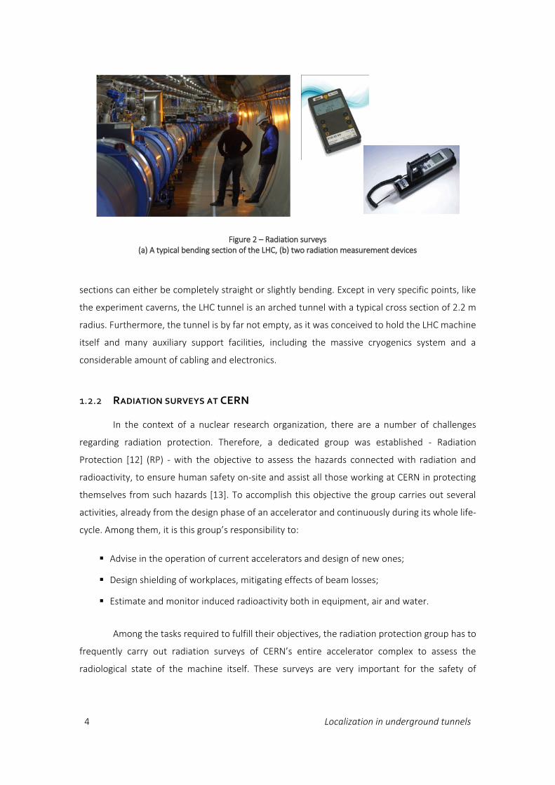
The LHC tunnel is divided into 8 octants or, alternatively, as 8 sectors, each one with a
specific purpose. Although it seems to follow a perfectly circular trajectory, the LHC tunnel’
Figure 1 - A geographical view of the LHC and its four detectors
4 Localization in underground tunnels
sections can either be completely straight or slightly bending. Except in very specific points, like
the experiment caverns, the LHC tunnel is an arched tunnel with a typical cross section of 2.2 m
radius. Furthermore, the tunnel is by far not empty, as it was conceived to hold the LHC machine
itself and many auxiliary support facilities, including the massive cryogenics system and a
considerable amount of cabling and electronics.
1.2.2 RADIATION SURVEYS AT CERN
In the context of a nuclear research organization, there are a number of challenges
regarding radiation protection. Therefore, a dedicated group was established - Radiation
Protection [12] (RP) - with the objective to assess the hazards connected with radiation and
radioactivity, to ensure human safety on-site and assist all those working at CERN in protecting
themselves from such hazards [13]. To accomplish this objective the group carries out several
activities, already from the design phase of an accelerator and continuously during its whole life-
cycle. Among them, it is this group’s responsibility to:
Advise in the operation of current accelerators and design of new ones;
Design shielding of workplaces, mitigating effects of beam losses;
Estimate and monitor induced radioactivity both in equipment, air and water.
Among the tasks required to fulfill their objectives, the radiation protection group has to
frequently carry out radiation surveys of CERN’s entire accelerator complex to assess the
radiological state of the machine itself. These surveys are very important for the safety of
Figure 2 – Radiation surveys (a) A typical bending section of the LHC, (b) two radiation measurement devices

Introduction 5
personnel as they ensure that any area of the tunnel is radiologically safe before access is granted.
In its basic form, the radiation survey teams, equipped with probes, measure the radiation levels
at specific points along the whole accelerator (see Figure 2). They record these values to evaluate
the risk a certain area presents and take the necessary actions.
1.2.3 THE RADIATION LOGGING PROJECT
Radiation surveys are a critical process for the CERN RP group. However, since several
measurements have to be taken every 100 m for nearly 30 km of tunnels, it represents a notorious
effort in terms of time and resources. Furthermore, as the collected information was previously
written to paper forms, further processing of this information required third party teams to look
up the data and feed it into their own software utilities. Besides slow, this process was naturally
cumbersome and highly error-prone. Additionally, given the amount of data, processing and
statistical analysis was rather limited beforehand.
To address these issues, the RP group has launched the Radiation Logging project with
the goal to design and implement a logging system for radiation surveys, applying state-of-the art
techniques for data acquisition, transmission, storage and retrieval.
In Figure 3 an overview of the Radiation Logging project is provided. The radiation data
measured by the detectors is expected to be collected to a mobile computer, eventually a tablet,
Figure 3 - An overview of the Radiation logging project
6 Localization in underground tunnels
which controls the detector and ensures the validity of the data. This device must provide an
interface so that a person can supervise the process. The information in then transferred to a
central database while eventually replicated for reasons of safety and availability. In the end, a
front-end interface provides the user with the tools to browse and create data analysis reports.
Such a system must face a large set of requirements and constraints, including:
A freely moving device which needs to be designed and read out continuously whilst
travelling by chariot or whilst being carried by a walking or cycling person;
It should automatically record as well as transfer all data on-the-fly via a wireless network
to a database;
The integrity of this data transfer has to be ensured in the very challenging environment
of several kilometers of underground tunnels while the measurement device is moving
at variable speed;
The measurements must be associated to a position which clearly identifies the place of
the measurement with a minimum of human intervention;
Data must be accessible through a user-friendly computer interface providing a geo-
referenced interactive map.
These requirements lead to three main areas of research, whose outcome must, in the
end, be part of a well-integrated system. These three areas comprise:
Positioning, as a novel approach for localization in such unique conditions, like the LHC
tunnel, must be developed and meet the stringent constraints that apply.
Data communication and storage, as we must ensure the validity and high-availability of
the data, even in case of system failure, yet meeting performance requirements.
Information technologies, enabling for a highly informative and user-friendly retrieval of
data, which must be synchronized with pre-existing systems, namely geo-localization
and machinery layout databases at CERN.
The Radiation Logging project introduces a wide range of challenges from very diverse
research areas, which go beyond the scope of a PhD research thesis. In the context of this thesis
one focuses on localization techniques, specially designed for the existing tunnel configuration.
Introduction 7
1.3 SCOPE OF THE THESIS
1.3.1 PROBLEM STATEMENT
In order to fulfil its goal, the project shall provide a set of positioning functionalities and
consider a set of restrictions in accordance to the context. An analysis of these factors lead to the
definitions of several high-level requirements. The localization solution to be developed must:
Provide localization coverage in the whole tunnel area while being cost effective;
Allow for accuracy levels capable of localizing multiple persons within a few tens of
meters, while being simple and resilient ;
Can optionally be upgraded in areas where higher accuracy levels are required, in the
order of one meter;
Integrate itself transparently with existing accelerator equipment and copes with tunnel
regulations;
Integrate easily with existing personnel activities and systems operations, namely the
radiation surveys. Such integration shall be as transparent as possible in order to help
reducing processes time so that the advantages in terms of safety are met.
For the moment this list of requirements is kept intentionally simple. A pragmatic
definition and identification of the requirements is given in 2.2.2 and 3.3.2 respectively.
1.3.2 PROPOSED SOLUTION
In the context of an accelerator tunnel, where the risk of hardware damage due to
radiation is high and the area to be localization-enabled is long, solutions requiring little or no
infrastructure changes are preferred. Therefore, the first part the study focus on localization
techniques based on the Received Signal Strength Indicator (RSSI) of the existing wireless
networks. Nevertheless, the existing scenario does not reflect the characteristics addressed in
most studies of the localization research community, such as Wireless LAN (IEEE 802.11) in an
office or shopping-mall. Instead, the area is covered with GSM network available throughout the
tunnel via a set of leaky-feeder cables.

8 Localization in underground tunnels
After the characterization of the RSSI profile, a method specifically developed for
localization along the tunnel is suggested. The method relies on analysis of RSSI fingerprints
collected all along the tunnel which are stored in a smart radio-map, and uses a variant of a k-
Nearest-Neighbors (KNN) algorithm to obtain the position within an acceptable range for safety
purposes, in the order of 50 m.
In order to further increase the accuracy, a second-stage method is proposed, which
allows to improve the accuracy from regions achieved by the RSSI method to sub-meter range.
This second-stage method is based on phase delay measurements of a VHF carrier injected in the
leaky-feeder and subsequent translation into a position in the given range.
1.3.3 ORIGINAL CONTRIBUTIONS
The scientific contributions yielding from this PhD work and described in this thesis are
introduced hereafter. They can be classified in two major groups:
Group 1 –Tunnel localization based on RSSI
Characterization of the Received Signal Strength Indicator (RSSI) profile of GSM signal
propagated over Leaky-Feeder cable along a long narrow tunnel.
To date and to our knowledge, this thesis includes the first studies characterizing the
propagation of GSM and WLAN signals over leaky feeder cable in a narrow tunnel as
long as 27 km. Besides found to be very sensitive to the presence of bodies, the RSSI for
each channel is affected independently, according to the different propagation paths.
A KNN-based localization algorithm for RSSI fingerprints.
A KNN algorithm was specifically designed to take advantage of multiple channels of the
GSM network, the signal variance at each sample and the fact that some channels had
propagated in opposite direction in the leaky-feeder cable. Furthermore, the algorithm
was implemented so that additional network signals can be taken into account,
including WLAN signals.
A framework for evaluation of fingerprinting localization algorithms supporting fusion
strategies of data originating from different technologies.
Introduction 9
A software suite was developed for efficient testing of localization algorithms over a
database of RSSI samples. The suite is optimized for large data sets and can take several
algorithms for different data sources, combining them according to a defined fusion
strategy. It also produces performance statistical indicators.
Group 2 – Enhancing localization accuracy with narrowband techniques
A localization algorithm for Software Defined Radios (SDR) based on carrier phase-delay
measurements.
The study shows that narrowband techniques can be successfully used for localization
in short ranges, even if there are obstacles, by leveraging the existence of a leaky-feeder
cable. The algorithm was specifically designed to operate on a Software-Defined-Radio
platform, taking its limitations into account.
The design of a hybrid localization solution.
The design of a localization system for the LHC tunnel which enhances the location
accuracy whenever requested in a high-precision enabled area.
1.4 THESIS STRUCTURE
The remaining part of this document is organized as follows. Chapter 2 gives an
introduction of general concepts used throughout the thesis, including wireless communications,
forms of communication in tunnels and basics of distance finding used for positioning. Chapter 3
provides a thorough overview of wireless positioning techniques and presents the state of the art
of solutions relevant to the current study, addressing in deeper detail those in which this work
builds on. Chapter 4 characterizes the tunnel’s RSSI profile from several temporal and spatial
perspectives. In chapter 5 the development of the first-stage localization solution is presented,
where the signal RSSI and new KNN variants are explored in single and multi-technology versions.
A localization software framework implemented for the purpose is also described. Chapter 6
presents the high-accuracy localization approach based on Round-trip Time-of-Flight (RTOF); the
approach is prototyped using Software-Defined-Radio (SDR) and tests regarding its feasibility in
the tunnel are shown.

10 Localization in underground tunnels

Wireless Localization Fundamentals 11
Chapter 2
WIRELESS LOCALIZATION FUNDAMENTALS
The fast-paced development of wireless communications and the proliferation of mobile
connected devices have driven the demand for accurate localization to very high levels.
Depending on the application, different location characteristics are required and many wireless
positioning technologies have to be taken into consideration. In general as higher levels are
demanded in the various dimensions of localization quality, more sophisticated processing
techniques are used as well as more precise measurements methods.
In the case of indoor environments, many challenging conditions and specific demands
apply. As such, a thorough understanding of the transmission medium is required so that
positioning technologies can be developed to specifically meet them.
2.1 THE “WIRELESS” CHANNEL
Since the ancient times of society, communication needs have always been among the
top priorities of society and, as a consequence, communication technology has been marked by
an impressive evolution and constant revolutions in its history. First wireless networks
transmitted information over line-of-sight (LOS) distances using smoke signals, and semaphore
signs. The invention of the telegraph, by Morse in 1838, and lately the telephone, by Bell in 1876,
came to revolutionize these means of communication by transmitting electrical signals over a
wired medium. Relatively fast communication over long distances was made possible.
This kind of transmission remained the only possibility until Marconi demonstrated the
first radio transmission in 1895. At the age of 21, after some modifications to his initial prototype,
he is able to communicate over a hill - a distance of 2.4 km (Marconi, 1909). Since then, the world
has witnessed one of the most impressive development in technology and industry success.
Cellular systems have experienced exponential growth over the last decade and there are

12 Localization in underground tunnels
currently around two billion users worldwide. Indeed, cellular phones have become a critical
business tool and part of peoples’ everyday life.
2.1.1 RADIO PROPAGATION
Wireless networks differ fundamentally from wired networks due to the unpredictable
and difficult nature of the wireless channel. As it propagates, the signal power varies as a function
of space, frequency and time. Besides attenuation (also known as Large-scale fading, or Slow-
fading), the particular conditions of the propagation path might favor reflection, refraction and
scattering effects so that even minor movements of the transmitter, receiver or surrounding
objects may considerably affect the transmission quality. Diffraction is the effect of “bending” the
propagation path on object corners, while Reflection happens when the signal hits a surface with
dimensions larger than its wavelength, and Scattering when the signal is “cut” by objects much
smaller than its wavelength. For a deeper insight on these effects refer, for example, to (Parsons,
2000) and (Goldsmith, 2005).
Radio propagation models try to assess the signal power evolution as a function of
distance, and usually combine empirical and analytical methods. Although analytical models are
provide adequate approximations in free-space and simpler propagation scenarios, they are
ineffective in estimating the power in a dense environment due to unpredictability of the effects
mentioned before (Latvala, et al., 2000). In turn, empirical models can be developed very fine-
grained, but their validity holds only for the same physical configuration and frequencies.
Path Loss
The fundamental estimation of the resulting signal strength of an electromagnetic wave
after travelling in free space, usually air, is known as Free-Space Path Loss (FSPL). It assumes no
obstacles and does not account for hardware imperfections. The premises for the equation are
that power loss is proportional to the square of the distance between transmitter and receiver,
and also proportional to the frequency of the signal.
𝑃𝑎𝑡ℎ𝐿𝑜𝑠𝑠 = (
4𝜋𝑑
𝜆)2
(eq. 2.1)
Wireless Localization Fundamentals 13
Equation yields the power attenuation coefficient, given the distance (d) and wavelength
(λ) in meters. It is often practical to obtain attenuation in dB’s, given the frequency in Hz and
distance in km. In that case the expression becomes:
𝑃𝑎𝑡ℎ𝐿𝑜𝑠𝑠𝑑𝐵 = 20 log10 𝑑 + 20 log10 𝑓 − 32.45 (eq. 2.2)
The path loss equations are used as a part of the Friis free-space model, which may take
transmitter and receiver antennas’ gain into account. This model is the basis for large-scale
propagation models but is only valid in the far-field of the transmission antenna. For shorter
paths, more realistic models exist, including the Hata-Okumura and the COST231-Hata models
(Rappaport, 1996), both to frequencies up to 2 GHz. For higher frequencies (Erceg, et al., 1999)
proposed a model which takes into consideration the type of terrain, the antenna dimensions
and a shadowing factor.
Shadowing
According to the path loss model, the power at a certain distance d from the transmitter
is a deterministic. However, it is known that for the same the distance point the power varies due
to reflection and diffraction by interfering objects along the path. These effects are in general
known as shadowing, and measurements show they can be modeled as a log-normally distributed
(normal in dB) random variable, i.e.:
𝜂𝑠ℎ𝑎𝑑_𝑑𝐵 ~ 𝑁𝑜𝑟𝑚(0, 𝜎𝑠ℎ𝑎𝑑) (eq. 2.3)
Shadowing (σ), at a distance of 100m, has typically values in the order of 6 dB.
Fast-Fading
Fast, or Small-Scale, fading is characterized by quick variations of the signal power over
short distances. This effect happens when the scattered signal components interfere among each
other, a mechanism known as Multipath Interference. Due to the different propagation paths,
they may present different amplitudes and phases and, if the phases are considerably different,
destructive addition takes place and a lower signal strength is measured. The impulse response
of a channel representing the sum of all the signal scattered components can be given by:

14 Localization in underground tunnels
ℎ(t) = ∑ 𝐴𝑚𝛿(𝑡 − 𝑡𝑚)
𝑁
𝑚=1
(eq. 2.4)
In (eq. 2.4) Am is the amplitude distortion and δ the Dirac delta function delayed by tm. In
the case of sinusoidal waves complete destruction occurs if two components have a phase shift
of π rad. Therefore, having approximately 3 m wavelength, 100MHz signals exhibit fast fading
phenomena in the meter range.
2.1.2 A SHARED MEDIUM FOR COMMUNICATIONS AND LOCALIZATION
Many other factors arise from the fact that air is a shared medium. First of all, the radio
spectrum is a scarce resource and, due to that, is controlled by regulatory bodies, both regionally
and globally. Second, security is also more difficult to implement since anybody can “listen” to
any communication in-range. Wireless networking is also significantly more challenging. Cellular
networks must be able to locate a given user wherever he is among billions of globally-distributed
mobile terminals and ensure transmission is kept possible even when the receiver is moving fast
and eventually traverses areas covered by different transmitters.
Wireless networks for communication
Cellular network systems were those which pushed for wireless revolution. Their main
purpose was to provide national and international coverage for bi-directional voice and data
communication. It is named after the network coverage layout, in which the Base Stations cover
a relatively small area, called cell, and several adjacent cells are required to properly cover a
geographical area. In this configuration frequencies can be reused in non-adjacent cells, leading
to better efficiency in spectrum use. While in first generation cellular systems (1G)
communication was analogue, second (2G) and third generation (3G) use digital transmission,
employing TDMA and CDMA multiplexing techniques.
Apart from the wide coverage of wireless networks and highly motivated by the advent
of fast Internet, the demand of limited-range high-speed wireless networks has steadily
increased. Wireless LANs started to appear in the early 1990's with data-rates on the order of 1-
2 Mbit/s. They operate in the unlicensed (ISM) frequency bands and, given the transmissions'
limited power, frequency allocation and regulation are no longer an issue. After the first
generation of such devices being incompatible among them, a set of standards have been

Wireless Localization Fundamentals 15
developed by the IEEE consortium, which have been adopted worldwide. In the first WLAN
standard, the IEEE 802.11 (IEEE, 1997), systems were specified with data rates up to 2 Mbit/s and
a range of approximately 150 m. The current standard IEEE802.11n (IEEE, 2009) specifies data
rates up to 600 Mbit/s by employing Multiple-Input Multiple-Output (MIMO) techniques,
considerable larger bandwidth channels (40 MHz), and several MAC layer optimizations.
Communication networks for positioning
Across times and technologies, wireless networks have been deployed with the main
purpose of providing data communication abilities to users. They focus, in the first place, on the
network characteristics perceived as quality parameters, such as data rate, range, mobility
support and fairness. Nevertheless, another use of the network has becoming increasingly
important. In 1996 the Federal Communications Commission in the U.S. introduced requirements
for wireless service providers being able to locate users within 100 meters in an emergency
situation (FCC, 1996); a similar directive was set to the European Union (EC, 2002). This concept
was later extended to Wireless LANs (WLANs) and high accuracy geo-localization technologies
started to be explored. These techniques can virtually turn any wireless network into a tracking
system for people and goods. They are primarily relevant for cellular network providers as a mean
to locate users and optimize the network performance. Nevertheless they can be used for a
myriad of applications, personal or industrial, where the location of something is to be monitored
or even automatically controlled.
The Global Positioning System - GPS
The most known and widely used positioning technique is that used by the GPS system
(GPS.gov, 2014), based on measurements of the signal delays - see part 2.3.1. The propagation
times of signals from satellites at known locations are measured simultaneously, and the distance
between a satellite and a user’s receiver is obtained by assessing the propagation time and
assuming LOS conditions. In many cases, however, the LOS signal is followed by multipath
components that arrive at the receiver with a delay, introducing significant changes into the signal
travelling time its gain estimation, especially in urban environments due to the many reflections
from buildings and other objects. For exactly those reasons GPS doesn’t work or performs poorly
in such environments.

16 Localization in underground tunnels
2.2 CLASSIFICATION OF POSITIONING SYSTEMS
There are several possibilities for classifying positioning systems, each of which making
use of different characteristics. Although it is common to characterize according to the
infrastructure underlying technology (e.g.: WLAN, Cellular, proprietary) or the signal used (e.g.:
infrared, sound, cameras), these types of classification are somewhat bound to a given domain
(e.g. Indoor localization - see section 3.2 from Chapter 3). However it is important to understand
its classification according to the topology, as it will define the system design.
2.2.1 CLASSIFICATION ACCORDING TO THE TOPOLOGY
In a classification according to the topology (Drane, et al., 1998), the entities Base-Station
(BS) and Mobile Station (MS) are defined and they might independently play the role of
“Obtaining” or “Using” the position information. In this definition is included the case they
perform both (“obtain and use”) or none of them (i.e.: localization passive). In such conditions,
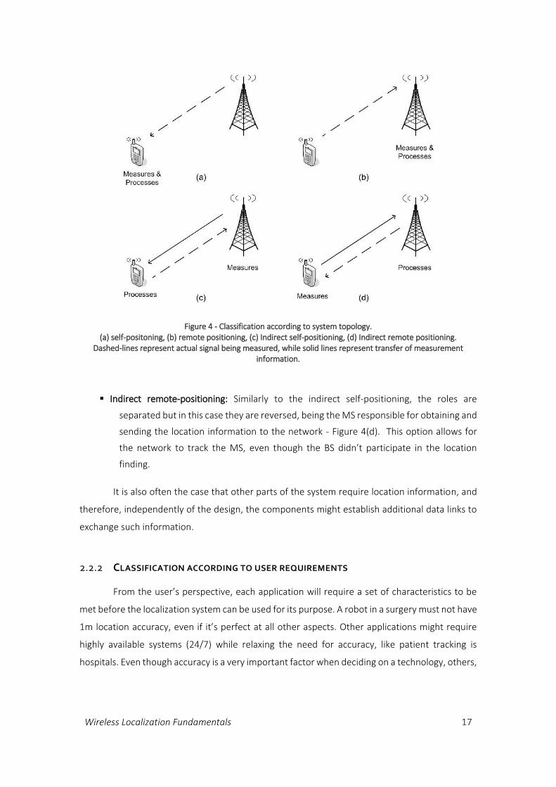
four scenarios are possible:
Self-positioning: The MS performs the signal measurements and processes them to obtain
the location - Figure 4(a). Such topology is quite common since it is well-adapted for
situations where positioning is not the primary goal of the network, although the MS
can still profit from the signal to infer location properties (e.g.: fingerprinting over
WLAN). Self-positioning is also the only viable solution for massive localization systems,
where communication with a BS would either create a bottleneck or be difficult, as in
the case of GPS. Self-positioning is a topology both scalable and simple, yet it has the
eventual disadvantage that the network does not know the positioning of the MS’s.
Remote positioning (or network-based positioning): The BS is responsible for calculating
the MS position based on the signal received directly or indirectly from it - Figure 4(b).
This is the case of typical tracking performed by cellular networks, where all the
information is generated on the network side but not available to the MS. Remote
positioning systems therefore suffer from poor scalability, while allowing for higher
integrity, privacy and performance from the operator point of view.
Indirect self-positioning: The BS calculates the position of the MS and sends to it the
location information via a data channel - Figure 4(c). This makes the location available
also to the MS even when it is technologically preferable to calculate the position in the
BS.
Wireless Localization Fundamentals 17
Indirect remote-positioning: Similarly to the indirect self-positioning, the roles are
separated but in this case they are reversed, being the MS responsible for obtaining and
sending the location information to the network - Figure 4(d). This option allows for
the network to track the MS, even though the BS didn’t participate in the location
finding.
It is also often the case that other parts of the system require location information, and
therefore, independently of the design, the components might establish additional data links to
exchange such information.
2.2.2 CLASSIFICATION ACCORDING TO USER REQUIREMENTS
From the user’s perspective, each application will require a set of characteristics to be
met before the localization system can be used for its purpose. A robot in a surgery must not have
1m location accuracy, even if it’s perfect at all other aspects. Other applications might require
highly available systems (24/7) while relaxing the need for accuracy, like patient tracking is
hospitals. Even though accuracy is a very important factor when deciding on a technology, others,
Figure 4 - Classification according to system topology. (a) self-positoning, (b) remote positioning, (c) Indirect self-positioning, (d) Indirect remote positioning.
Dashed-lines represent actual signal being measured, while solid lines represent transfer of measurement information.
18 Localization in underground tunnels
depending on the context, might even be more important. In the end all must be taken into
account with their own priority.
According to the work by Mautz (2012) there are 16 kinds of requirements, which can be
perceived as 16 dimensions defining the characteristics of a system:
Accuracy / Uncertainty – “Positioning accuracy” should be perceived as the degree with
which an estimated position matches the true value at a given time, which is usually
calculated at a confidence level of 95%. This term is being deprecated in favor of
“Measurement Uncertainty”, well defined by the Joint Committee for Guides in
Metrology (JCGM) in JCGM 200:2008 (2008).
Coverage area – Refers to the spatial extension the system operates in, while guaranteeing
specifications. Three broad classifications exist: Local coverage, Scalable coverage and
Global coverage.
Cost – Cost is always an important requirement, which for the case of positioning systems
has to be assessed in several perspectives, including initial deployment, per user/device
cost, extension and maintenance effort.
Infrastructure – The required infrastructure will mostly impact the initial deployment
effort and, if required, can be passive or active, dense or sparse, dedicated or leveraging
another.
Market maturity – Whether the technology is a concept, being developed or a proven
product.
Output data – The output might be simply a set of 1-, 2- or 3-D coordinates, but additional
parameters might be useful in some situations, including velocity and uncertainty
assessments.
Privacy – Whether the determined positions should be available to the user itself only, a
set of authorized operators, or publicly shared among all users.
Update rate – Update rate can vary from the position being calculated every few days to
elevated rates (e.g.: hundreds of hertz for a robot arm).
Interface – Shall the system provide human-machine interfaces (e.g. a GUI) or machine
interface only (e.g.: Rest API’s, protocol over the network, serial).
Wireless Localization Fundamentals 19
System integrity – The possibility to evaluate the quality of an estimate (output) and alert
the user if the error exceeds a defined limit. This might be a critical factor for safety
systems.
Robustness – Relates to which degree the system can cope with harsh operating
conditions and protection against misuse, theft or jamming.
Availability – Encompasses the number of requests the system can process and the error
frequency and recoverability, measured by requests-per-second, mean-time-between-
failures and percentage of up-time.
Scalability – The possibility of the system to gradually increase its availability or coverage
area, which can come at additional costs or detriment of other properties (e.g.:
accuracy).
Number of users – Whether the system is operated by a single user (e.g. robot), supports
multiple users up to infrastructure saturation, or accepts unlimited users thanks to a
decentralized design (e.g.: passive sensors).
Intrusiveness / User acceptance – The degree to which the system integrates the
environment and is adapted to the involved processes, and can range from
imperceptible to disturbing.
Approval – Some systems might be subject to approval and certification both at the local
level (company internal regulations) and obeying national legal regulations (e.g.
electromagnetic power emission levels).
These parameters pose a multidimensional optimization problem to the system to be
built. Having in mind that no system can perform exceptionally in all requirements, a careful
assessment of the priorities is a key step during its design phase, which will define some of the
fundamental aspects, including the technology.
2.3 WIRELESS DISTANCE MEASUREMENTS
Within the positioning domain, one can identify two concepts that are closely related:
distance measurement and location. While the first aims at determining the distance between
two objects, the latter deals with objects as a point in geo-referenced coordinates system.
20 Localization in underground tunnels
Nevertheless, distances can help us to determine a location and, the other way round, it is
possible to calculate the distance between two referenced locations. After these, other measures
can further be calculated, namely velocity and acceleration. Nevertheless, one must not overlook
that time dependent measures are susceptible to errors due to delays introduced in the
measurement process.
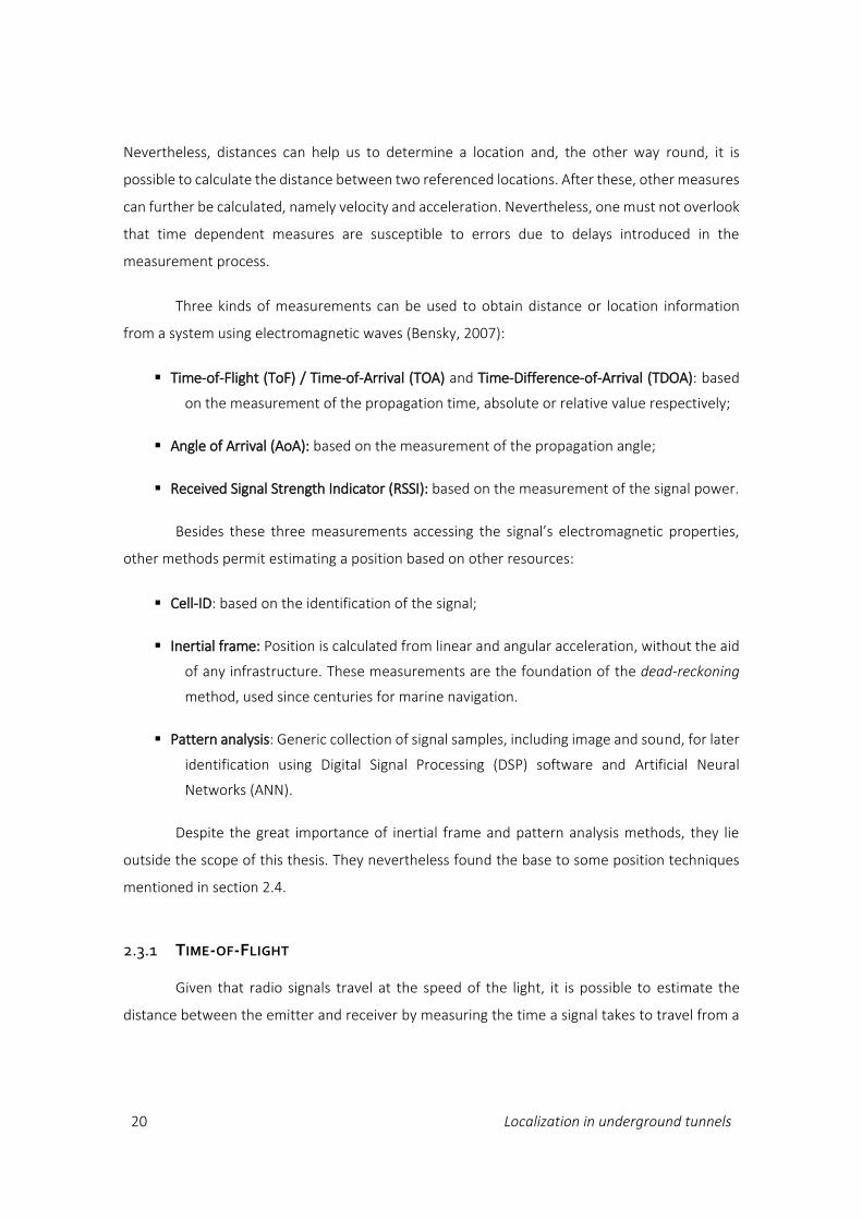
Three kinds of measurements can be used to obtain distance or location information
from a system using electromagnetic waves (Bensky, 2007):
Time-of-Flight (ToF) / Time-of-Arrival (TOA) and Time-Difference-of-Arrival (TDOA): based
on the measurement of the propagation time, absolute or relative value respectively;
Angle of Arrival (AoA): based on the measurement of the propagation angle;
Received Signal Strength Indicator (RSSI): based on the measurement of the signal power.
Besides these three measurements accessing the signal’s electromagnetic properties,
other methods permit estimating a position based on other resources:
Cell-ID: based on the identification of the signal;
Inertial frame: Position is calculated from linear and angular acceleration, without the aid
of any infrastructure. These measurements are the foundation of the dead-reckoning
method, used since centuries for marine navigation.
Pattern analysis: Generic collection of signal samples, including image and sound, for later
identification using Digital Signal Processing (DSP) software and Artificial Neural
Networks (ANN).
Despite the great importance of inertial frame and pattern analysis methods, they lie
outside the scope of this thesis. They nevertheless found the base to some position techniques
mentioned in section 2.4.
2.3.1 TIME-OF-FLIGHT
Given that radio signals travel at the speed of the light, it is possible to estimate the
distance between the emitter and receiver by measuring the time a signal takes to travel from a
Wireless Localization Fundamentals 21
point to another, i.e., transmitter to receiver. The time, t, the signal will arrive to the receiver is
given by:
t = t𝑇𝑋 +
𝑑
𝑐+ 𝑑𝑇 (eq. 2.5)
In (eq. 2.5) tTX is is transmission time, d the distance and c the speed of light. dT is a term
to stand for clock drifts, which must be considered if the send/receive devices are not completely
synchronized.
A prime and well-known application of this concept is radar. Modern tracking and missile
control radars use the monopulse technique (U.S. Naval Research Laboratory, 1943) in which, in
its basic form, a device emits a radio frequency pulse and measures the time elapsed until the
reflected pulse is acquired by the receiver device. The distance is then calculated based on the
pulse’s propagation speed, usually the speed of the light, and the fact that the pulse travels forth
and back, i.e. double the distance between the objects. In these systems, the accuracy is
proportional to its time resolution which, in turn, is proportional to clock frequency.
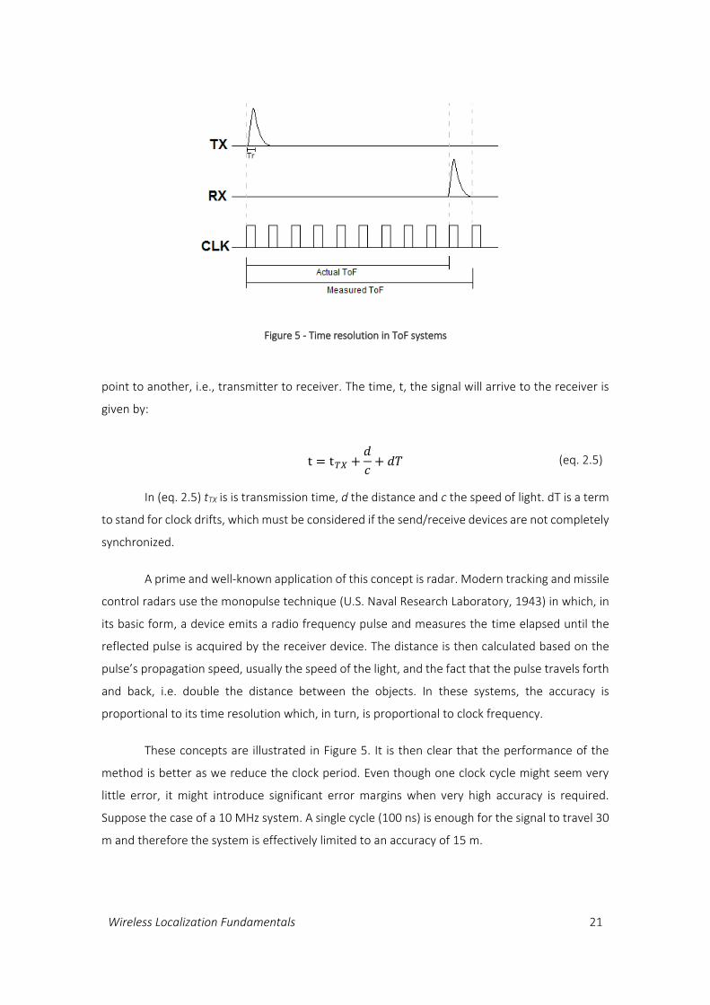
These concepts are illustrated in Figure 5. It is then clear that the performance of the
method is better as we reduce the clock period. Even though one clock cycle might seem very
little error, it might introduce significant error margins when very high accuracy is required.
Suppose the case of a 10 MHz system. A single cycle (100 ns) is enough for the signal to travel 30
m and therefore the system is effectively limited to an accuracy of 15 m.
Figure 5 - Time resolution in ToF systems
22 Localization in underground tunnels
Another aspect is that the pulse width must be narrow enough to allow for an adequate
detection. On the one hand we must ensure that no pulse echo is received while it is still being
transmitted and, on the other hand, multiple reflections of the pulse should be distinguishable
among them so that one can clearly identify the first reflection and infer the shortest path. The
pulse rise time 𝑇𝑟 depends directly on the signal bandwidth 𝐵 which, for a square wave, is given
by:
𝑇𝑟 =
1
𝐵 (eq. 2.6)
The technique of measuring a reflected signal, as employed in radar, implicitly solves a
commonly complex problem: the need for device synchronization. Since the transmitter and
receiver devices are together they can share the clock reference and, therefore, it is
straightforward to assess the correct travel time. In the case of a decoupled design, where the
transmitter can’t be physically connected to the receiver, a mechanism for very-precise clock
synchronization must be in place. In order to avoid the synchronization problem, another
technique is often explored - TDoA.
2.3.2 TIME-DIFFERENCE-OF-ARRIVAL
Several reasons can be behind a decoupled design despite the complex problem it
introduces: the need for a simple receiver, a noisy and/or high-attenuation transmission medium,
scalability requirements, etc. TDoA takes into consideration additional signal sources to avoid the
need for absolute clocks by measuring the relative delay between signals. This process usually
allows to calculate the clock drift and to synchronize the units as well.
GPS is a prime example of a TDoA systems, where all the previously mentioned conditions
apply. It finds the location by solving a system of typical ToF equations contemplating a clock-drift
term, requiring information from at least four satellites (Langley, 1991).
Synchronized transmitters, unknown clock-drift
When measuring distance, basic ToF accounts for unknown distances only which can
therefore solved using simple motion equations. When inserting a clock-drift (dT) term, additional
information must be added to the system so it can be solved.

Wireless Localization Fundamentals 23
One of the most popular techniques is to install an additional transmitter, which is
synchronized to the first unit. Both units then transmit signals, either simultaneously or with
known delay among them, so that the receiver is able to determine the propagation times and
even to correct its clock drift.
Consider the situation where the distance between a BS and a MS is to be calculated.
With the aid of a second transmitter in line1, if both send a synchronized pulse, the time at the
receiver shall respect a system of equations based on (eq. 2.5) 1:
{𝑡1 = 𝑡𝑇𝑋1 +
𝑑1
𝑐+ 𝑑𝑇
𝑡2 = 𝑡𝑇𝑋2 +𝑑2
𝑐+ 𝑑𝑇
(eq. 2.7)
Since dT depends on the receiver, tTX2 = tTX1 + K where K constant, and defining Δt = t1-
t2, one obtains:
Δ𝑇 =
𝑑1
𝑐−𝑑2
𝑐− 𝐾 (eq. 2.8)
Finally, being an infrastructure, the distance between the transmitters is known.
Therefore D=d1+d2 1, yielding the solutions:
𝛥𝑇 =
2. 𝑑1 − 𝐷
𝑐− 𝐾
⇒ {
𝑑1 = 𝐷 + 𝑐. (𝛥𝑇 + 𝐾)
2
𝑑𝑇 = 𝑡1 − 𝑡𝑇𝑋1 +𝑑1
𝑐
(eq. 2.9)
As seen in (eq. 2.9), the distances can be calculated based on the measured ΔT and
system known constants. For clock synchronization to be possible the only condition would be to
calculate dT by having access to tTX1. This could be accomplished by encoding tTX1 and transmitting
it in the signal itself. Clock synchronization is also performed in GPS and indeed most receivers
automatically set their date/time based on the network. For higher dimensions, in 2- and 3-D
spaces, the process is called Multilateration, and is described in section 2.4.2.
1 The case of 1D requires transmitters is opposite sides of the receiver. For higher dimensions see 2.4.2
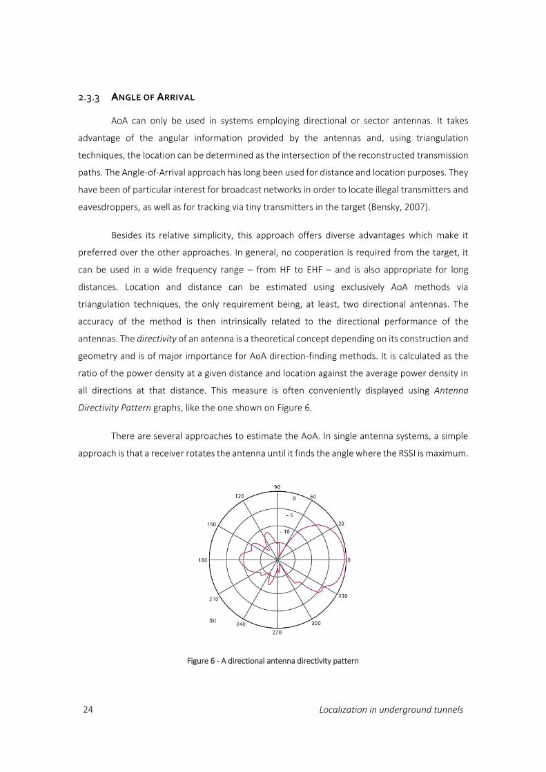
24 Localization in underground tunnels
2.3.3 ANGLE OF ARRIVAL
AoA can only be used in systems employing directional or sector antennas. It takes
advantage of the angular information provided by the antennas and, using triangulation
techniques, the location can be determined as the intersection of the reconstructed transmission
paths. The Angle-of-Arrival approach has long been used for distance and location purposes. They
have been of particular interest for broadcast networks in order to locate illegal transmitters and
eavesdroppers, as well as for tracking via tiny transmitters in the target (Bensky, 2007).
Besides its relative simplicity, this approach offers diverse advantages which make it
preferred over the other approaches. In general, no cooperation is required from the target, it
can be used in a wide frequency range – from HF to EHF – and is also appropriate for long
distances. Location and distance can be estimated using exclusively AoA methods via
triangulation techniques, the only requirement being, at least, two directional antennas. The
accuracy of the method is then intrinsically related to the directional performance of the
antennas. The directivity of an antenna is a theoretical concept depending on its construction and
geometry and is of major importance for AoA direction-finding methods. It is calculated as the
ratio of the power density at a given distance and location against the average power density in
all directions at that distance. This measure is often conveniently displayed using Antenna
Directivity Pattern graphs, like the one shown on Figure 6.
There are several approaches to estimate the AoA. In single antenna systems, a simple
approach is that a receiver rotates the antenna until it finds the angle where the RSSI is maximum.
Figure 6 - A directional antenna directivity pattern
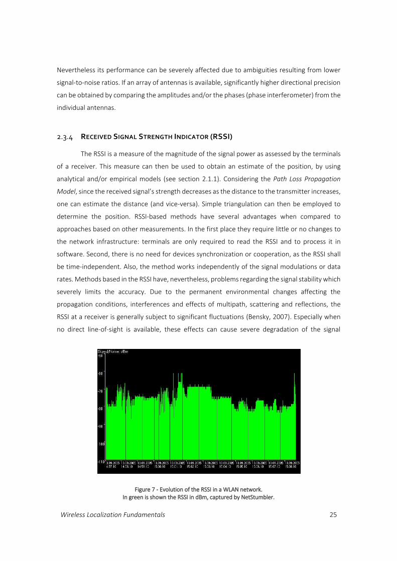
Wireless Localization Fundamentals 25
Nevertheless its performance can be severely affected due to ambiguities resulting from lower
signal-to-noise ratios. If an array of antennas is available, significantly higher directional precision
can be obtained by comparing the amplitudes and/or the phases (phase interferometer) from the
individual antennas.
2.3.4 RECEIVED SIGNAL STRENGTH INDICATOR (RSSI)
The RSSI is a measure of the magnitude of the signal power as assessed by the terminals
of a receiver. This measure can then be used to obtain an estimate of the position, by using
analytical and/or empirical models (see section 2.1.1). Considering the Path Loss Propagation
Model, since the received signal’s strength decreases as the distance to the transmitter increases,
one can estimate the distance (and vice-versa). Simple triangulation can then be employed to
determine the position. RSSI-based methods have several advantages when compared to
approaches based on other measurements. In the first place they require little or no changes to
the network infrastructure: terminals are only required to read the RSSI and to process it in
software. Second, there is no need for devices synchronization or cooperation, as the RSSI shall
be time-independent. Also, the method works independently of the signal modulations or data
rates. Methods based in the RSSI have, nevertheless, problems regarding the signal stability which
severely limits the accuracy. Due to the permanent environmental changes affecting the
propagation conditions, interferences and effects of multipath, scattering and reflections, the
RSSI at a receiver is generally subject to significant fluctuations (Bensky, 2007). Especially when
no direct line-of-sight is available, these effects can cause severe degradation of the signal
Figure 7 - Evolution of the RSSI in a WLAN network. In green is shown the RSSI in dBm, captured by NetStumbler.
26 Localization in underground tunnels
stability with notorious implications on the positioning accuracy. Figure 7 shows the RSSI in dBm
for a WLAN network. Notice that fluctuations are as high as 20dB, i.e., a factor of 100.
Analytical and empirical approaches
Two main approaches are used for the estimation: analytical or empirical. Analytical
approaches make use of the radio propagation models. Therefore obtaining the position becomes
as simple as solving the loss equations in respect to the distance and inputting the measured
power. The Free Space Model (eq. 2.1) is definitely a reference for such estimation, in the form
that it is used to calculate a constant component, which depends on the distance. To account for
this stochastic behavior of the received power as shown before, the most generic approach is
then to consider all these effects as single additive Gaussian-distributed components with a given
standard deviation σshad, as:
RSSI = p0 − 10β log 𝑑 + 𝑛𝑠ℎ𝑎𝑑 , 𝑛𝑠ℎ𝑎𝑑 ~ 𝑁𝑜𝑟𝑚(0, 𝜎𝑠ℎ𝑎𝑑) (eq. 2.10)
In (eq. 2.10) it is given that the RSSI directly depends on the transmitted power p0
subtracted a path loss component with distance d and loss exponent β, and a random loss nshad.
Other models try to express the propagation characteristics of more elaborate environments,
including indoor locations. Despite their simplicity, these methods can indeed work well as long
as they accurately reflect the real propagation conditions. This situation is, unfortunately, very
hardly the case of indoor scenarios, where a large shadowing component has generally to be
introduced, which is a direct source of distance error. Analytical approaches remain, therefore,
an option almost exclusive to outdoors and other simple environments, where line-of-sight is
available with little multipath and reflection conditions.
For applications, including positioning, requiring an accurate characterization of the
signal strength in a complex space, empirical approaches have been explored. A possibility is to
measure the signal strength at a set of predefined locations to create a map of the network, which
can be later tested for similarities with new samples. These techniques are denominated of
Fingerprinting, and are described in more detail in section 2.5.

Wireless Localization Fundamentals 27
2.4 POSITION FINDING TECHNIQUES
Positioning is typically performed by processing several measurements, as described in
the previous section, and often, on a combination of some of them. In this section we provide an
overview of the basic positioning techniques, including proximity and multilateration methods,
as well as some extended information on Fingerprinting.
2.4.1 PROXIMITY SENSING
Amongst the simplest location finding principles, proximity sensing does not require the
measurement of signal between the parties. Instead, it is based on the identification of the signal
which, in cellular-style networks, translates into a certain location region defined by the network
coverage.
Proximity methods in cellular GSM networks
Cellular networks have been intrinsically able to localize terminals with this method by
using the Cell-ID, more specifically, the GSM channel identification.
Even though they are generally straightforward, due to the large area covered by a single
network cell, especially in rural areas – up to 30 km, the positioning error can also be very
significant. To improve this figures a variant of the method, known as virtual center, calculates
the position as the central point among all the detected cells’ positions (Cheng, et al., 2005) which
can optionally be inversely averaged by their radii:
X =∑ 1
𝑟𝑖⁄ 𝑋𝑖𝑁𝑖=1
∑ 1𝑟𝑖⁄
𝑁𝑖=1
(eq. 2.11)
In a project involving localization of mobile units for assessing road traffic in Duisburg,
Germany (Jung, et al., 2009), by approximately calculating the cell’s geometry by identifying the
signal from adjacent BTS and using the antennas’ directional capabilities, an accuracy better than
477 m was found for 67% of the cases.
Without further analysis of the signal characteristics, as seen in the next part, little further
optimization can be done. Nevertheless this method finds its usefulness mostly for networks
where, the cell size is natural or intentionally kept small. This can be the case of micro- (radius:
28 Localization in underground tunnels
200-2000 m), pico GSM cells (radius: 4-200 m) (Linnartz, 1993), or dense coverage with other
networks.
Proximity methods in other networks - RFID
Despite the wide application of this method to cellular networks, these methods have
been explored for other standardized networks, including Bluetooth (standardized as IEEE
802.15), WLAN (IEEE 802.11) and proprietary systems. The basic principle is always applicable:
localization is defined to be that of the cell(s) in range. For a finer accuracy other signal properties
are used for sub-cell localization, mainly power and direction.
Due to its relatively low cost, and eventually making use of passive elements, a very dense
network of RFID tags could enable localization with good accuracy levels (relative to the network
density) in situations where GPS is not enough or not even available, like tunnels, indoors and
dense urban areas. An experiment by (Chon, et al., 2004) shows that information from RFID tags
combined with GPS and gyroscopes allow for accurate localization of vehicles in roads, even when
they are moving over 100 km/h. See section 3.5.1 for more details.
2.4.2 MULTILATERATION
The basic mechanisms to determine the location either use distances, angles or a
combination of both. In some cases, distances and angles can only be given in relative values, but
the ambiguity can be resolved with the help of additional sources of information.
Trilateration
Trilateration is a geometric process which determines positions from regions defined by
one of more circles. In terms of positions, a distance value only represents the radius of a
circumference where the receiver might be located. If one additionally knows the distance to a
second reference point, the intersection points of the circumferences might be calculated and
we end up with two single possible positions, as exemplified in Figure 8.
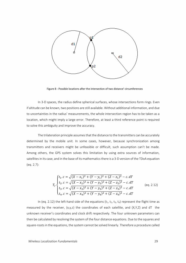
Wireless Localization Fundamentals 29
In 3-D spaces, the radius define spherical surfaces, whose intersections form rings. Even
if altitude can be known, two positions are still available. Without additional information, and due
to uncertainties in the radius’ measurements, the whole intersection region has to be taken as a
location, which might imply a large error. Therefore, at least a third reference point is required
to solve this ambiguity and improve the accuracy.
The trilateration principle assumes that the distance to the transmitters can be accurately
determined by the mobile unit. In some cases, however, because synchronization among
transmitters and receivers might be unfeasible or difficult, such assumption can’t be made.
Among others, the GPS system solves this limitation by using extra sources of information,
satellites in its case, and in the base of its mathematics there is a 3-D version of the TDoA equation
(eq. 2.7):
𝑇𝑟
{
𝑡1. 𝑐 = √(𝑋 − 𝑥1)
2 + (𝑌 − 𝑦1)2 + (𝑍 − 𝑧1)
2 − 𝑐. 𝑑𝑇
𝑡2. 𝑐 = √(𝑋 − 𝑥2)2 + (𝑌 − 𝑦2)
2 + (𝑍 − 𝑧2)2 − 𝑐. 𝑑𝑇
𝑡3. 𝑐 = √(𝑋 − 𝑥3)2 + (𝑌 − 𝑦3)
2 + (𝑍 − 𝑧3)2 − 𝑐. 𝑑𝑇
𝑡4. 𝑐 = √(𝑋 − 𝑥4)2 + (𝑌 − 𝑦4)
2 + (𝑍 − 𝑧4)2 − 𝑐. 𝑑𝑇
(eq. 2.12)
In (eq. 2.12) the left-hand side of the equations (t1, t2, t3, t4) represent the flight time as
measured by the receiver, (x,y,z) the coordinates of each satellite, and (X,Y,Z) and dT the
unknown receiver’s coordinates and clock drift respectively. The four unknown parameters can
then be calculated by resolving the system of the four distance equations. Due to the squares and
square-roots in the equations, the system cannot be solved linearly. Therefore a procedure called
Figure 8 - Possible locations after the intersection of two distance' circumferences
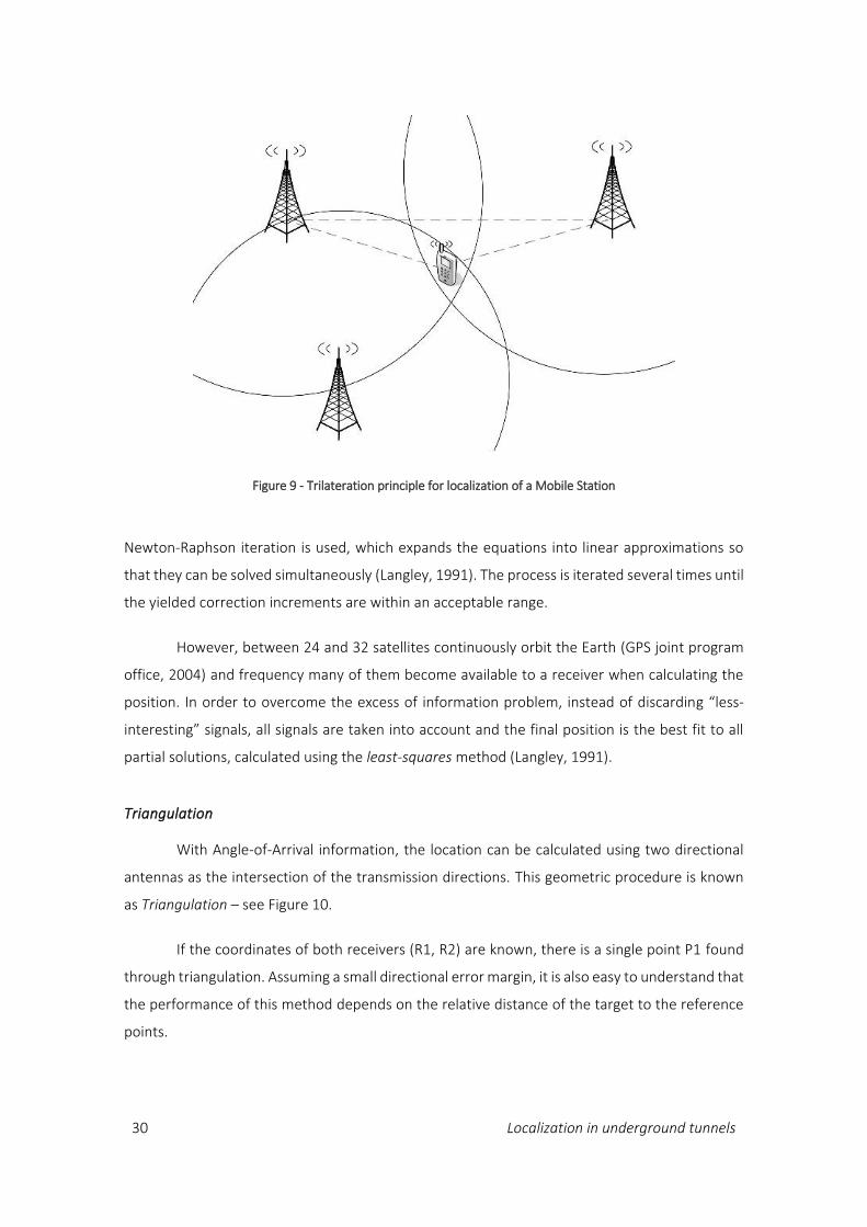
30 Localization in underground tunnels
Newton-Raphson iteration is used, which expands the equations into linear approximations so
that they can be solved simultaneously (Langley, 1991). The process is iterated several times until
the yielded correction increments are within an acceptable range.
However, between 24 and 32 satellites continuously orbit the Earth (GPS joint program
office, 2004) and frequency many of them become available to a receiver when calculating the
position. In order to overcome the excess of information problem, instead of discarding “less-
interesting” signals, all signals are taken into account and the final position is the best fit to all
partial solutions, calculated using the least-squares method (Langley, 1991).
Triangulation
With Angle-of-Arrival information, the location can be calculated using two directional
antennas as the intersection of the transmission directions. This geometric procedure is known
as Triangulation – see Figure 10.
If the coordinates of both receivers (R1, R2) are known, there is a single point P1 found
through triangulation. Assuming a small directional error margin, it is also easy to understand that
the performance of this method depends on the relative distance of the target to the reference
points.
Figure 9 - Trilateration principle for localization of a Mobile Station

Wireless Localization Fundamentals 31
Based on the principles of Euclidean geometry, distance d can be calculated from the
trigonometric relations of the distance between R1 and R2 and the angles made with P1, as:
𝑅1𝑅2̅̅ ̅̅ ̅̅ ̅ =𝑑
tan 𝛼+
𝑑
tan𝛽 (eq. 2.13)
Resolving to d, using the trigonometric identities tan(α) = sin(α)/cos(α) and sin(α + β) =
sin(α) cos(β) + cos(α) sin(β), we end up with:
𝑑 = 𝑅1𝑅2̅̅ ̅̅ ̅̅ ̅sin 𝛼 sin 𝛽
sin(𝛼 + 𝛽) (eq. 2.14)
With the distance d defined the position of P1 can be easily calculated. In a 2-D plain, one
approach is to calculate the distance 𝑅1𝑃̅̅ ̅̅ ̅ and translate α into the geographical absolute angle
αabs, so that the P coordinates are given by
𝑃 = 𝑅1 + 𝑅1𝑃̅̅ ̅̅ ̅. ⟨cos 𝛼𝑎𝑏𝑠 , sin 𝛼𝑎𝑏𝑠⟩ (eq. 2.15)
It is also of interest the case when both the direction and the distance are known by the
receivers, therefore making (eq. 2.15) directly applicable. In such situations, since both
measurements are complementary and sufficient to define a point in a referential, only one
receiver is actually necessary - see Figure 11.
Figure 11 - Location finding using Angular and distance information
Figure 10 - Estimating location via the intersection of AoA information

32 Localization in underground tunnels
Nevertheless, both capabilities don’t have necessarily to be in the same device. In some
systems the target can actually perform one of the measurements. For instance in cellular
networks, it’s actually the terminal which monitors the signal strength, while the angular
information and processing is performed on the base station.
Due to the simple infrastructure this system requires, it is actually used in a number of
applications, including very high frequency omnidirectional ranging (VOR) navigation, wildlife
tracking and article location in warehouses (Bensky, 2007).
2.4.3 DEAD-RECKONING
Dead-reckoning is a technique that calculates the current position based on the previous
ones, updating it based on the information coming from different sensors, namely speedometers,
accelerometers and gyroscopes. It has been widely used in the past, namely in marine navigation,
but its use is broad and has been applied to aeronautical, automotive and, more recently, robotic
and pedestrian navigation (Nebot, 1999) (Fang, et al., 2005). The dead-reckoning concept is often
the base of more complex algorithms, such as the Kalman filter used in fingerprinting.
Given that nowadays smartphone devices can have a number of built-in sensors, these
methods are well suited for enabling localization for the mobile device. As the principal
advantage, they are completely independent of any infrastructure and, once calibrated, they can
provide very accurate positing information in virtually real-time. The disadvantage of the method
stems from its principle, which accumulates values with error over time. Especially for those cases
where only acceleration measurements are available, since double-integration is performed to
obtain the position, enormous deviations from the real position very soon appear if speed and
position are not “fixed”. In many applications GPS is employed to correct these errors, being
successfully used as a source of so-called position fixes; however, this possibility is subject to the
availability of the GPS signal, which can’t be assumed for many scenarios, including indoors and
underground. For those cases additional fix sources are required, which can be accomplished with
the aid of pedometers (Randell, et al., 2003), magnetometers (Goyal, et al., 2001) and existing
network infrastructures, e.g. Wireless Sensor Networks (WSN’s) (Gadeke, et al., 2011). Dead-
Reckoning is referenced due to its importance to localization in general; however it lies outside
the scope of the current research.
Wireless Localization Fundamentals 33
2.5 LOCATION FINGERPRINTING TECHNIQUES
Location fingerprinting is an empirical method of estimating the location of a Mobile
Station which requires neither an exclusive infrastructure nor cooperation between the parties.
Location fingerprinting methods have been widely used indoors with RSSI measurements due to
their complex variability patterns which, for the most cases, are almost impossible to predict. Due
to their flexibility, fingerprinting methods can also be employed to AoA and ToA but their
applications is rather limited to specific situations. Furthermore, these methods have recently
received much attention regarding pattern analysis with imaging and sound signals. Despite
interesting, these applications lie outside the scope of this thesis.
Location fingerprinting methods involve an offline (or calibration) phase and an online (or
location estimation) phase. The offline phase consists in measuring the network signal
characteristics, also known as fingerprints, at certain calibration points in order to create a map
of the network. This map, called radio-map, can then be used during the online phase to infer the
position of the device, in a procedure involving comparing the newly collected signal
characteristics against those stored in the map. This characteristic makes fingerprinting to work
best for locations where the space complexity imposes deep changes in the signal that makes
each calibration point unique (Bensky, 2007).
Several fingerprinting methods exist and they can fall into one out of two categories
(Honkavirta, 2008):
Static location estimation algorithms: the fingerprints are individually used in the calculus
of a location. They can be further divided into Deterministic or Probabilistic algorithms.
Filtering algorithms. In this approach, the radio-map captures the relations among the
calibration points, making it more robust against measurement-wide variations.
Calibration phase
The radio-map is created during the calibration phase and is used for every location
estimation process. It stores the RSSI values of the signal as a function of their location within an
area of interest. Signal-to-Noise Ratio (SNR) data is also available but is usually disregarded since
the RSSI has a stronger correlation to the location (Bahl & Padmanabhan, 2000). In addition, some
factors that can strongly influence the readings are also registered. For instance, the orientation
34 Localization in underground tunnels
of the measurement since, due to human body shielding, can reduce the RSSI by 5 dB (Bahl &
Padmanabhan, 2000).
Given that different devices may report slightly different RSSI values, the calibration
process is performed utilizing the same device for the concerning area, which is also preferably
the one used during the online phase. In such circumstances, the RSSI becomes a relative
indicator, whose unit and eventual calibration factors introduced by the device are not relevant.
Nevertheless the RSSI values are normally given in power units, either mW or dBm.
During the calibration process, from tens up to thousands of samples are taken to
characterize each location. In order to reduce the computational demand it is useful, and
sometimes required, to preprocess the calibration map to reduce the amount of information to
be stored. The stored approximations will depend on the estimation methods used, the most
common being their statistical properties: Mean, Variance, Median, or a full Histogram. The
simplest approach is to store only the mean value, as used in the RADAR system (Bahl &
Padmanabhan, 2000). Despite being convenient, this approach completely discards the signal
variability, which might help characterizing the location profile. To mitigate that (Kaemarungsi &
Krishnamurthy, 2004) suggest to store the variance in addition to the mean, and assume the
samples to follow a Gaussian distribution.
In some scenarios, the RSSI distribution can be considered itself as a good characteristic
of the calibration points. In order to capture this information, (Roos, et al., 2002) propose storing
a histogram of the RSSI. Histograms are then the base of some probabilistic methods, as discussed
below.
2.5.1 DETERMINISTIC LOCATION ESTIMATION
In a deterministic approach, estimation is based on the similarity of a measurement and
the collected fingerprints. Normally, each measured fingerprint is evaluated independently and
the similarity to a given point of the radio-map is assessed by the norm of a distance vector,
calculated for N channels according to a norm p, as:
‖𝑥‖𝑝 = (∑|𝑥𝑖|
𝑝
𝑁
𝑖=1
)
1𝑝⁄
, 𝑥 = (�̅� − 𝑎�̅�) (eq. 2.16)

Wireless Localization Fundamentals 35
In (eq. 2.16) y is the vector of measured RSSI’s, and aj the vector of RSSI of an arbitrary
point j of the radio-map. For the case of Wireless LAN, each access point (AP) typically provides a
channel which, if measureable, represents an additional dimension to the distance vector. The
most common norms, p as in (eq. 2.16), are 1-norm (sum, also known as Manhattan distance), 2-
norm (Euclidean distance) and ∞-norm (maximum). The Euclidean distance is the most used one
for location fingerprinting (Honkavirta, 2008).
Another norm which is often used in fingerprinting is the Mahalanobis norm. It is defined
as the distance of a sample to a distribution defined by the means and deviations of a sample
vector (Mahalanobis & Chandra, 1936), formulated as:
𝐷𝑀(𝑥) = √(𝑥 − 𝜇)
𝑇𝜎−1. (𝑥 − 𝜇) (eq. 2.17)
Where σ is the covariance matrix and u the vector with the mean values for each channel.
Reformulating (eq. 2.17) considering individual RSSI samples, we obtain:
‖𝑥‖𝑀 = √𝑥
𝑇𝜎−1𝑥 (eq. 2.18)
For better understanding, (eq. 2.18) means that the Mahalanobis norm between two
points is the distance x among the points, in vectorial form, squared and weighted by the
covariance matrix. In case the covariance is the identity matrix, then it is equivalent to the
Euclidean norm.
Nearest Neighbor (NN) and K-Nearest Neighbor (KNN) methods
The Nearest Neighbor (NN) (Duda, et al., 2000) is one of the simplest methods for pattern
matching, hence used for location finding as well. It works by selecting from the radio-map the
point whose norm to the online measurement is smallest, i.e., the point having the closest RSSI
value, considered all the channels. Due to its simplicity, however, the method disregards
information of the other points with similar characteristics. Even though this might be desirable
and working best in some situation (Li, et al., 2006), the method could potentially fall in a local
optimum, yielding a solution which is far from the actual position.
To avoid this limitation, the K-NN method (or simply KNN) takes into account the K most
similar fingerprints from the radio-map. The location estimate (𝑥,̂ �̂�) is then calculated by an
36 Localization in underground tunnels
averaging process which, in its basic form, is given by the arithmetic mean of their coordinates
(𝑥𝑖 , 𝑦𝑖) (Lin & Lin, 2005), as:
(𝑥,̂ �̂�) =
1
𝑘∑(𝑥𝑖 , 𝑦𝑖)
𝐾
𝑖=1
(eq. 2.19)
Several modifications to the KNN approach exist in the literature, one of the most
relevant being the Weighted KNN. Is this approach the K selected fingerprints are given different
weights according to the method. For instance, (Li, et al., 2006) propose to use weights as the
inverse of the RSSI distance norm, as:
(𝑥,̂ �̂�) =
1
∑ 𝑤𝑖𝐾𝑖=1
∑𝑤𝑖(𝑥𝑖 , 𝑦𝑖)
𝐾
𝑖=1
(eq. 2.20)
where 𝑤i =1
‖𝑋𝑖‖ (eq. 2.21)
In (eq. 2.21) ‖Xi‖ is the distance, as defined in (eq. 2.16). The authors report that the
method performs better than the simple NN (K=1), yielding the best results for K=3 or K=4. For
higher values of K it is generally accepted that the method starts performing worse, as points
further away are considered and corrupt the averaging (Honkavirta, 2008).
2.5.2 PROBABILISTIC LOCATION ESTIMATION
One of the main drawbacks of the KNN methods is that they don’t take into consideration
extended information at each simple point, other than a single value, typically mean or median.
Such simplification typically disregards the variance, a key indicator of the quality of the sampling
and a characteristic of the position (Prasithsangaree, et al., 2002).
The objective of probabilistic methods is to determine the likelihood that the new
measurement belongs to a group of signal samples of the fingerprint, characterized by their
probability density function (pdf). Such testing is performed based on the Bayes’ theorem, and
therefore probabilistic methods are also known to follow the Bayesian framework.
𝑃(𝑥|𝑦) =
𝑃(𝑦|𝑥) 𝑃(𝑥)
𝑃(𝑦) (eq. 2.22)
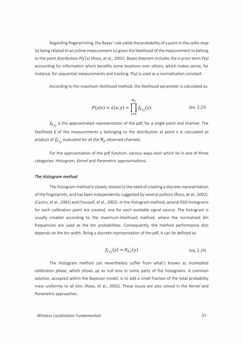
Wireless Localization Fundamentals 37
Regarding fingerprinting, the Bayes’ rule yields the probability of a point in the radio-map
(x) being related to an online measurement (y) given the likelihood of the measurement to belong
to the point distribution P(y│x) (Roos, et al., 2002). Bayes theorem includes the a-priori term P(x)
accounting for information which benefits some locations over others, which makes sense, for
instance, for sequential measurements and tracking. P(y) is used as a normalization constant.
According to the maximum likelihood method, the likelihood parameter is calculated as:
𝑃(𝑦|𝑥) = ℒ(𝑥; 𝑦) =∏𝑓𝑉𝑥𝑗(𝑦)
𝑁𝑦
𝑗=1
(eq. 2.23)
𝑓𝑉𝑥𝑗 is the approximated representation of the pdf, for a single point and channel. The
likelihood ℒ of the measurements y belonging to the distribution at point x is calculated as
product of 𝑓𝑉𝑥𝑗 evaluated for all the 𝑁𝑦 observed channels.
For the approximation of the pdf function, various ways exist which lie in one of three
categories: Histogram, Kernel and Parametric approximations.
The Histogram method
The histogram method is closely related to the need of creating a discrete representation
of the fingerprints, and has been independently suggested by several authors (Roos, et al., 2002),
(Castro, et al., 2001) and (Youssef, et al., 2002). In the Histogram method, several RSSI histograms
for each calibration point are created, one for each available signal source. The histogram is
usually created according to the maximum-likelihood method, where the normalized bin
frequencies are used as the bin probabilities. Consequently, the method performance also
depends on the bin width. Being a discrete representation of the pdf, it can be defined as:
𝑓𝑉𝑥𝑗(𝑦) = 𝐻𝑥,𝑗(𝑦) (eq. 2.24)
The Histogram method can nevertheless suffer from what’s known as incomplete
calibration phase, which shows up as null bins in some parts of the histograms. A common
solution, accepted within the Bayesian model, is to add a small fraction of the total probability
mass uniformly to all bins (Roos, et al., 2002). These issues are also solved in the Kernel and
Parametric approaches.
38 Localization in underground tunnels
The Kernel method
The kernel density method or Parzan window is another non-parametric method for
approximating the underlying probability density function (pdf) of the samples. The method is, by
definition, more precise since it doesn’t have to “round” a sample to fit a specific bin, but the
original sample value is taken into account, and, therefore it is widely used for data interpolation.
The approximation is a continuous distribution and, therefore, it allows the result to be calculated
analytically, while avoiding the problem with empty bins.
The approximation to the pdf is defined by the averaging of so-called kernel functions.
Each Kernel is the continuous representation of a sample, approximated to a parametric
distribution, whose center is the average of the sample (Roos, et al., 2002).
𝑓𝑉𝑥,𝑗(𝑦) =
1
𝑁∑
1
𝑉𝑁 𝐾𝑥,𝑗 (
𝑦 − 𝑦𝑖ℎ𝑛
)
𝑁
𝑖=1
(eq. 2.25)
In (eq. 2.25) N is the number of sample groups, between 1 and the sample count, Vn is
the sample volume, hn the group normalized width or window size, and Kx,j is the kernel function
chosen for the point and channel.
A number of parametric distributions can be used as kernel functions, the most common
being Normal/Gaussian, Log-normal and Exponential (Honkavirta, et al., 2009).
To help understanding the approximation performed by Kernel method and the influence
of the parameters window size (hn) and sample groups (N), consider the distribution represented
by Figure 12, a bi-modal distribution. The representation is obviously perfectly with infinite
samples; however, using a small number of samples, the results depend very much on the
parameters. For instance, when only a single sample is used, the approximation to the first mode
is good (hn=5), but the second mode is completely lost. This fact raises the awareness that, the
more appropriate the kernel function used, the lower the number of samples required to
reasonably represent the actual pdf.

Wireless Localization Fundamentals 39
Parametric methods
In a parametric approach the RSSI histograms are approximated to some known
distribution. By using the pdf of a known distribution, the computing of the likelihood becomes
simple. Nevertheless, since the RSSI is so highly affected by the space, obtaining good results with
this method is a challenging task. The two most common approximations are Gaussian and Log-
normal distributions.
The use of the Gaussian distribution to approximate RSSI pdf’s has been applied in several
works (Haeberlen, et al., 2004; Li, et al., 2006; Kaemarungsi, 2006). However, despite its success,
the Gaussian distribution is symmetric and might not capture the RSSI distribution of weaker
signals, which frequently exhibit a long tailed shape. In those situations the log-normal
distribution might be more suitable (Honkavirta, et al., 2009).
Figure 12 - Pdf approximation by kernel method with Gaussian functions. Plots for different window’ and sample sizes

40 Localization in underground tunnels
2.5.3 THE FILTERING APPROACH
A different approach to fingerprinting is to consider all the previous measurements in
addition to the current one, when calculating the location estimate. Filtering techniques try to
capture eventual patterns in the signal variations and use it to better match measured points in
the online phase. The use of the earlier measurements is based on the state model, where the
state of the previous measurement is matched with the current one, accounting for some state
and measurement noise generally with zero mean. Although the time-series analysis might
require significantly higher computation power, the methods provide better position accuracy
than static location estimation (Honkavirta, 2008). Two important filters exist in the literature:
the Bayesian filter and the Kalman filter.
Bayesian filter
The Bayesian filter is the natural extension of the probabilistic approach. It builds exactly
on the same base (eq. 2.22), but in this case the a-priori term P(x) has now a full meaning: the
probable previous positions to help deciding the next position (Honkavirta, et al., 2009). Defining
the time index k, the Bayes’ expression becomes
𝑃(𝑥𝑘|𝑦1:𝑘) =
𝑃(𝑦𝑘|𝑥𝑘) 𝑃(𝑥𝑘|𝑦1:𝑘−1)
𝑃(𝑦𝑘|𝑦1:𝑘−1) (eq. 2.26)
As seen in (eq. 2.26), the probability for a given position at time k (xk) is calculated given
all the performed measurements until the current ones (y1:k). After an initialization state, as
required by any state model, two phases follow cyclically: the prediction and the update. The
prediction refers to the calculation of the a-priory term, while the update phase is the actual
resolution of the Bayes’ rule, which accounts equally for the likelihood 𝑃(𝑦𝑘|𝑥𝑘) but also to the
conditional probability of being in that position given the previous measurements (the a-priory
term). The calculation of the a-priori is usually done using the Chapman-Kolmogorov equation
(Gardiner, 1985) which introduces a transition density term, accounting for the probability of a
next state (or position) to be chosen given the previous one. This term can be modeled as a matrix
of probabilities of transitions between cells and, interestingly, this matrix can be defined based
on the adjacent cells’ information from the building floor’s plan (Honkavirta, et al., 2009).
Wireless Localization Fundamentals 41
Kalman filter
If Kalman filter (Grewal & Andrews, 2001; Kalman, 1960; Kailath, et al., 2000) is one of
most well-known filters which, in recursive manner, estimates past, present and future states of
an unknown noisy process. Due to its flexibility and relatively low computational requirements, it
has been successfully applied to a number of research areas, with special emphasis on tracking
of moving devices.
The Kalman filter (KF), in is fact an implementation of the Bayesian filter and, accordingly,
it works in two phases: prediction and update. However, the filter assumes that the models used
in the prediction and update phases are linear, and the noise follows Gaussian distribution, i.e.,
white noise.
Several extensions to the KF have been proposed, some of them tackling the linearity
restriction. The most used solutions are the Extended Kalman Filter (EKF), described in detail by
(Grewal & Andrews, 2001), and the Unscented Kalman Filter (UKF) proposed by (Julier &
Uhlmann, 1997). In both cases, the approach is to approximate the non-linear term by Taylor
series expansion; but while the EFK approximates the models with the first derivative, the UFK
does the approximation using the second derivative.
A comparison on the performance of the Kalman filter and its EFK and UFK variants
regarding mobile navigation is provided by (Ali-Loytty, et al., 2005). For more detail on the filters
regarding localization the reader can also refer to (Honkavirta, 2008) and (Figueiras & Frattasi,
2010).
42 Localization in underground tunnels
2.6 SUMMARY
Chapter 2 introduced the fundamentals of localization in general. It started by discussing
the opportunities and challenges of the wireless medium, which had been mostly exploited for
data transmission but the same principles apply and have been researched for localization as well.
In this part the most important factors impacting performance are also discussed: Path loss,
Shadowing and Fast fading. This part is followed by two classifications of positioning systems, one
based on their topology and another based on the functional requirements.
In part 2.3 the several wireless distance measurement principles are introduced. They
can be generally categorized according to some transmission property, either propagation time,
propagation angle, power loss or even the reach to nearby receivers. These measurements are
the pillar for position finding techniques discussed in part 2.4. Among them, fingerprinting
techniques have become very popular, as they work for a number of signals and network types,
including sound or image matching, and especially with the Received Signal Strength to perform
localization. Due the rich diversity of these methods, part 2.5 is entirely dedicated to them,
covering deterministic methods, probabilistic or Bayesian approaches and some filters that are
also used for localization purposes.

Indoors and Underground Positioning 43
Chapter 3
INDOORS AND UNDERGROUND
POSITIONING
Despite the good performance and acceptance of global satellite-based (GNSS) and many
outdoor location technologies in general, the ability for these systems to perform similarly well –
if at all possible – indoors, remains a constant challenge.
Even though the same principles apply for both indoors and outdoors, their performance
will greatly vary, a fact closely tied to the substantial differences the environments exhibit and
the distinct applications they should serve.
This chapter discusses applications of indoor positioning, followed by a summary of
technologies and techniques that allow communication and localization indoors, with emphasis
on underground environments.
3.1 APPLICATIONS OF INDOOR POSITIONING
In indoor situations GNSS and other outdoor location technologies are not a viable
solution. Furthermore many applications require an accurate, fast, and flexible positioning,
tracking and navigation functions.
On the other hand, the possibility of locating indoors allows for a set of applications that
wouldn’t be possible otherwise, which promise to substantially change our lives for more
comfort, safety and eventually entertainment, including the following:
Location-based Services (LBS) – services that provide information relative to the current
geographical positions. Examples are hand-held devices that show contents as the user moves,
like a navigation system outdoors, or a museum guide in indoors.

44 Localization in underground tunnels
Assistance in Private Homes – These include applications ranging from the tracking of
objects’ position to the motion of people. Examples are controlling TVs with gestures,
finding lost keys or even Ambient Assisted Living (AAS), where elderly people are
monitored in the event of accident or health crisis.
Assistance in Health Institutions – The fast location of personnel in hospital and health
centers has become of major importance, mostly in urgencies, and for patients in case
of sudden severe problems. Moreover, precise positioning is required for robots
assisting during surgeries.
Environment Monitoring – Some activities require the monitoring of physical properties of
materials and infrastructures, like temperature, pressure, deformation. These
properties can be measured by grids of sensors forming so-called Wireless Sensor
Networks that can calculate positions using cooperative algorithms.
Safety and Rescue – Indoor position capabilities can be of extreme importance for
coordination of safety and rescue operations by the police or fire brigades. Besides the
location of the emergency team elements, the tracking of workers in hazardous areas
might show to be extremely useful in speeding up assistance in case of an accident.
Transportation – Automated driving and guided parking might be doing their first steps
thanks to properly equipped cars and parking garages.
Industry – Many mechanical processes of assemblage and displacement will benefit from
better positioning in order to become more automated. One of the most notable
examples are assembly lines of car manufacturing industry.
Logistics and optimization – tracking the position of goods and personnel enables the fast
retrieval/routing of goods and allocation of people to the respective process. If required
the process might be optimized by relative closeness. Such optimization is key in
logistics centers, but can also improve efficiency in administrative businesses, where
documents have to be tracked and processed.
Underground activities – Tunnels, mines and other underground facilities are often
environments of extreme conditions (dust, darkness, humidity, instability and/or
irregularity of walls) and therefore hazardous for workers. Localization plays a central
role for safety although it might also improve the industrial process in cause, like the
installation of equipment.
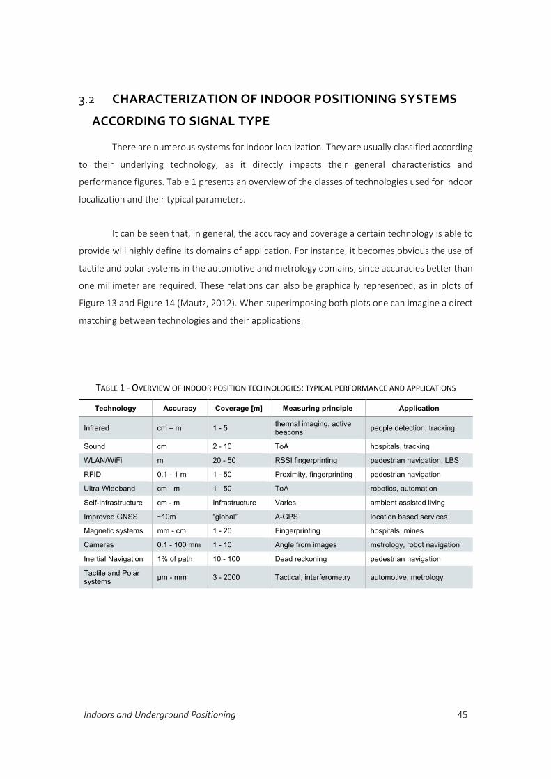
Indoors and Underground Positioning 45
3.2 CHARACTERIZATION OF INDOOR POSITIONING SYSTEMS
ACCORDING TO SIGNAL TYPE
There are numerous systems for indoor localization. They are usually classified according
to their underlying technology, as it directly impacts their general characteristics and
performance figures. Table 1 presents an overview of the classes of technologies used for indoor
localization and their typical parameters.
It can be seen that, in general, the accuracy and coverage a certain technology is able to
provide will highly define its domains of application. For instance, it becomes obvious the use of
tactile and polar systems in the automotive and metrology domains, since accuracies better than
one millimeter are required. These relations can also be graphically represented, as in plots of
Figure 13 and Figure 14 (Mautz, 2012). When superimposing both plots one can imagine a direct
matching between technologies and their applications.
TABLE 1 - OVERVIEW OF INDOOR POSITION TECHNOLOGIES: TYPICAL PERFORMANCE AND APPLICATIONS
Technology Accuracy Coverage [m] Measuring principle Application
Infrared cm – m 1 - 5 thermal imaging, active beacons
people detection, tracking
Sound cm 2 - 10 ToA hospitals, tracking
WLAN/WiFi m 20 - 50 RSSI fingerprinting pedestrian navigation, LBS
RFID 0.1 - 1 m 1 - 50 Proximity, fingerprinting pedestrian navigation
Ultra-Wideband cm - m 1 - 50 ToA robotics, automation
Self-Infrastructure cm - m Infrastructure Varies ambient assisted living
Improved GNSS ~10m “global” A-GPS location based services
Magnetic systems mm - cm 1 - 20 Fingerprinting hospitals, mines
Cameras 0.1 - 100 mm 1 - 10 Angle from images metrology, robot navigation
Inertial Navigation 1% of path 10 - 100 Dead reckoning pedestrian navigation
Tactile and Polar systems
µm - mm 3 - 2000 Tactical, interferometry automotive, metrology

46 Localization in underground tunnels
Figure 13 - Technologies according to coverage and accuracy levels
Figure 14 - Localization applications according to required coverage and accuracy
Indoors and Underground Positioning 47
In the case of underground constructions, in order to meet the suggested accuracy levels
(0.1 to 10 cm) and coverage requirements (10 to 100 m), magnetic, sound, pseudo-lites and Ultra
Wide Band (UWB) technologies are typically used. However, from the given information, there is
no single technology which fully meets these requirements, even though only a pair (of
requirements) was specified. Furthermore, as stated before, these parameters depend on the
specific application, and therefore a comprehensive analysis is required.
3.3 CHALLENGES INDOORS AND IN UNDERGROUND MEDIUM
Indoor localization can be particularly challenging for several reasons, arising from the
fact that there are walls and objects around the confined spaces where transmission is to occur
(Mautz, 2012).
These conditions favor several signal effects, which are unusually undesirable as they
highly impact on the measured signal properties, including propagation delay and the power. In
particular, from those presented in Chapter 2 section 2.1, the following effects are particularly
significant:
Multipath due to signal reflection
Non-Line-of-Sight (NLoS) due to signal blockage and reflection
High Attenuation due to distances and obstacles
Scattering due to different material densities traversed
Dynamic conditions, due to the movement of people and objects
The large majority of positioning technologies have been designed for indoor
environments; however most existing commercial products have been developed for use in office
buildings, airports, shopping malls, factory plants, and other similar spaces. Nevertheless these
solutions usually don’t meet the requirements for underground scenarios, which present distinct
properties and challenges.
3.3.1 UNDERGROUND MEDIUM PROPERTIES
Underground tunnels and mines, or even underwater wells and caves, present a very
particular scenario when compared to surface and other indoor environments. They are
48 Localization in underground tunnels
structurally different and offer different conditions in terms of localization opportunities. Still,
tracking and navigation for such spaces play a central role for safety and in rescue operations, as
well as for supporting specific activities or for scientific research activities in other fields.
These spaces are particularly difficult scenarios for radio transmission, a fact that has
been observed since the 1920’s following the boom in mining activity. Such difficulty is associated
with their physical characteristics which have a negative effect in the transmission of
electromagnetic waves (Delogne, 1991), the most significant being:
confined spaces encompassed by irregular surfaces
circular or rectangular tunnel sections
presence of halls, cross-cuts and blockages
Limited Line-of-Sight (LOS)
Presence of ionized air, humid and warm conditions
Presence of additional gases
Structural changes
In such conditions, comparing to indoors, the adversities on the transmission of wireless
signals are further emphasized:
Extreme path-loss: high losses due to material absorption and humidity.
Reflections and Refractions: Due to proximity of the walls, reflection effects can be quite
strong, resulting in a waveguide effect. Furthermore, because of the irregular nature of
the walls, reflections can be quite distorted which will turn into noise.
Multipath fading: the random combination of multiple propagation paths leads to fast
variations in the signal strength. Hence, this effect is also known as fast-fading.
Dynamic conditions: Besides the movability of people and objects, the tunnel dielectric
properties (permittivity and permeability) change with the temperature. As a
consequence, besides different propagation paths, also the propagation speed is
subject to variations.
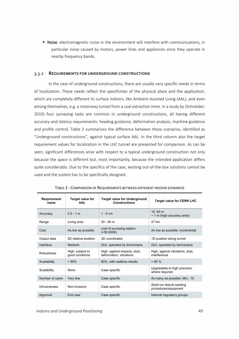
Indoors and Underground Positioning 49
Noise: electromagnetic noise in the environment will interfere with communications, in
particular noise caused by motors, power lines and appliances since they operate in
nearby frequency bands.
3.3.2 REQUIREMENTS FOR UNDERGROUND CONSTRUCTIONS
In the case of underground constructions, there are usually very specific needs in terms
of localization. These needs reflect the specificities of the physical place and the application,
which are completely different to surface indoors, like Ambient Assisted Living (AAL), and even
among themselves, e.g. a motorway tunnel from a coal extraction mine. In a study by (Schneider,
2010) four surveying tasks are common in underground constructions, all having different
accuracy and latency requirements: heading guidance, deformation analysis, machine guidance
and profile control. Table 2 summarizes the difference between those scenarios, identified as
“Underground constructions”, against typical surface AAL. In the third column also the target
requirement values for localization in the LHC tunnel are presented for comparison. As can be
seen, significant differences arise with respect to a typical underground construction not only
because the space is different but, most importantly, because the intended application differs
quite considerably. Due to the specifics of the case, existing out-of-the-box solutions cannot be
used and the system has to be specifically designed.
TABLE 2 - COMPARISON OF REQUIREMENTS BETWEEN DIFFERENT INDOOR SCENARIOS
Requirement name
Target value for AAL
Target value for Underground Constructions
Target value for CERN LHC
Accuracy 0.5 - 1 m 1 - 5 cm 10 -50 m ~ 1 m (high accuracy area)
Range Living area 20 - 50 m 27 km
Cost As low as possible cost of surveying station (<50.000€)
As low as possible, incremental
Output data 2D relative position 3D coordinates 1D position along tunnel
Interface Network GUI, operated by technicians GUI, operated by technicians
Robustness High, subject to good conditions
High, against impacts, dust, deformation, vibrations
High, against vibrations, dust, interference
Availability > 90% 80%, with realtime results > 95 %
Scalability None Case specific Upgradable to high precision where required.
Number of users Very few Case specific As many as possible. Min.: 10
Intrusiveness Non-invasive Case specific Shall not disturb existing procedures/equipment
Approval End user Case specific Internal regulatory groups

50 Localization in underground tunnels
3.4 TECHNOLOGIES FOR UNDERGROUND COMMUNICATIONS
Although tunnels do, to a certain extent, propagate wireless signals, it may be very
difficult to predict the signal characteristics after a few hundred meters. Even if regular signal
measurements were performed to assess these characteristics, network planning would become
a laborious task and, moreover, many situations would still impose serious obstacles to natural
propagation, including non-continuous tunnel sections, very irregular surfaces, caverns, water
leaks. Because of these problems, new communication techniques have been developed that
cope with such inhospitable underground characteristics.
Underground communication techniques can be classified according to the main
underground medium used (Bandyopadhyay, et al., 2010): Through-the-Air (TTA), Through-the-
Wire (TTW) and Through the Earth (TTE)
3.4.1 THROUGH-THE-AIR (TTA)
TTA communications comprise a whole set of radio techniques which don’t require any
specific propagation medium, other than air. Natural propagation is a primary means of
communication which, besides all limitations, can be adequate for regular shaped tunnels or
specific applications. There are mostly two techniques:
1. Free tunnels as waveguides - Using the tunnel itself to guide the waves.
2. Wireless Mesh networks - In which several access points cooperate to create a resilient
and wide coverage network.
Free tunnels as waveguides
In an empty tunnel, propagation behaves similarly to that occurring in hollow waveguides
(Chiba, et al., 1978) in which only frequencies above a threshold imposed by the tunnel size and
shape will propagate properly. This frequency is known as the cut-off frequency of the medium,
for which the standard equations for metallic waveguides still provide good approximations.
According to propagation laws in circular waveguides, the cut-off frequency for the
dominant mode TE11 is given by

Indoors and Underground Positioning 51
𝑓𝑐𝑚𝑛𝑇 =
χ𝑇𝑚𝑛2𝜋𝑟√𝜇휀
⇒ 𝑓𝑐11𝑇𝐸 =
1.8412 . c
2𝜋𝑟 (eq. 3.1)
Thus, the relation of the cut-off wavelength and the waveguide radius can be expressed
as:
𝑐
𝜆𝑐=1.8412 . c
2𝜋𝑟 ⇒ 𝜆𝑐 ≈ 0.3𝑟 (eq. 3.2)
This relation confirms the rough approximation of both parts having the same order of
magnitude, many times used as a reference in tunnels.
Propagation of waves whose frequency is above cut-off is known as Natural Propagation:
𝜆 ≤ 0.3𝑟 ⇒ 𝑓 ≥
𝑐
0.3𝑟 (eq. 3.3)
Experimental works in (Chiba, et al., 1978) show that the tunnel diameter should be from
several to ten times larger than the free-space wavelength for natural propagation to occur. For
instance, in a tunnel of 2 m diameter, 500MHz signals are expected to “naturally” propagate well.
Wireless Mesh Networks (WMN)
A new approach to TTA has been explored for tunnel communications based on the
development of specialized Wireless Mesh Networks. Cooperative networking techniques have
been successfully applied to tunnels and underground facilities, defining a field denominated as
Wireless Underground Communication Networks (WUCNs) (Akyildiz, et al., 2009). These
networks consist of wireless devices that operate below the ground surface which are either (i)
buried completely under dense soil or (ii) placed within a limited open underground space such
as mines and road/subway tunnels. Clearly taking advantage of the ever less expensive network
elements, this approach focuses on the devices’ cooperation to form a network with remarkable
resiliency features. According to propagation medium, they fall undoubtedly in the TTA and TTE
categories.
3.4.2 THROUGH-THE-WIRE (TTW)
TTW techniques require some wired communication infrastructure. Twisted pair, Coaxial
cable, CAT5/CAT6, trolley cable, optical fiber and leaky-feeder are some of the most used types of
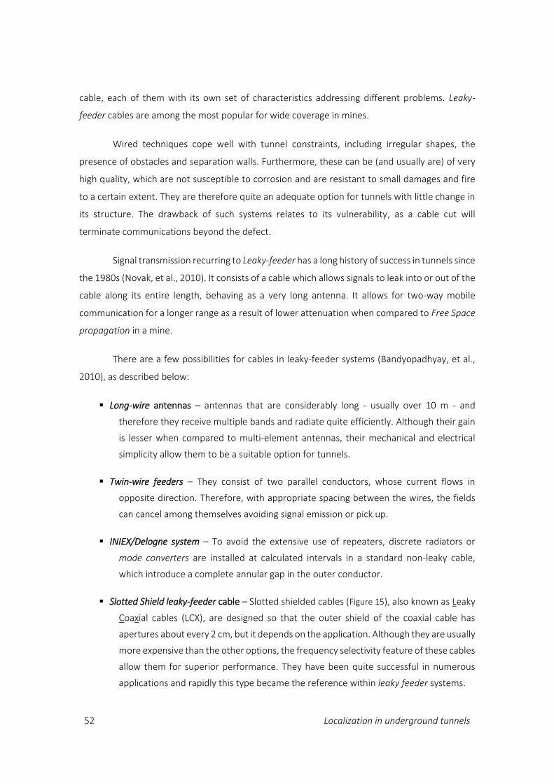
52 Localization in underground tunnels
cable, each of them with its own set of characteristics addressing different problems. Leaky-
feeder cables are among the most popular for wide coverage in mines.
Wired techniques cope well with tunnel constraints, including irregular shapes, the
presence of obstacles and separation walls. Furthermore, these can be (and usually are) of very
high quality, which are not susceptible to corrosion and are resistant to small damages and fire
to a certain extent. They are therefore quite an adequate option for tunnels with little change in
its structure. The drawback of such systems relates to its vulnerability, as a cable cut will
terminate communications beyond the defect.
Signal transmission recurring to Leaky-feeder has a long history of success in tunnels since
the 1980s (Novak, et al., 2010). It consists of a cable which allows signals to leak into or out of the
cable along its entire length, behaving as a very long antenna. It allows for two-way mobile
communication for a longer range as a result of lower attenuation when compared to Free Space
propagation in a mine.
There are a few possibilities for cables in leaky-feeder systems (Bandyopadhyay, et al.,
2010), as described below:
Long-wire antennas – antennas that are considerably long - usually over 10 m - and
therefore they receive multiple bands and radiate quite efficiently. Although their gain
is lesser when compared to multi-element antennas, their mechanical and electrical
simplicity allow them to be a suitable option for tunnels.
Twin-wire feeders – They consist of two parallel conductors, whose current flows in
opposite direction. Therefore, with appropriate spacing between the wires, the fields
can cancel among themselves avoiding signal emission or pick up.
INIEX/Delogne system – To avoid the extensive use of repeaters, discrete radiators or
mode converters are installed at calculated intervals in a standard non-leaky cable,
which introduce a complete annular gap in the outer conductor.
Slotted Shield leaky-feeder cable – Slotted shielded cables (Figure 15), also known as Leaky
Coaxial cables (LCX), are designed so that the outer shield of the coaxial cable has
apertures about every 2 cm, but it depends on the application. Although they are usually
more expensive than the other options, the frequency selectivity feature of these cables
allow them for superior performance. They have been quite successful in numerous
applications and rapidly this type became the reference within leaky feeder systems.
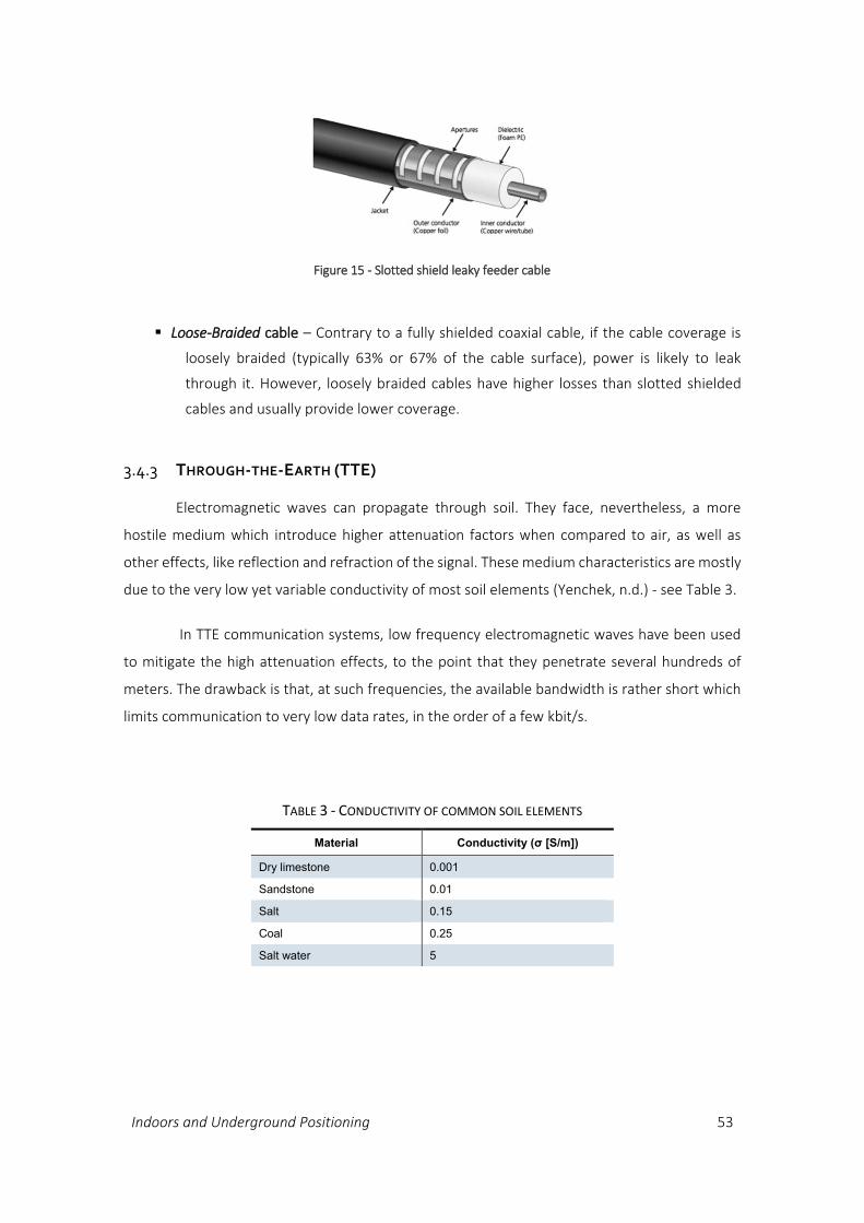
Indoors and Underground Positioning 53
Loose-Braided cable – Contrary to a fully shielded coaxial cable, if the cable coverage is
loosely braided (typically 63% or 67% of the cable surface), power is likely to leak
through it. However, loosely braided cables have higher losses than slotted shielded
cables and usually provide lower coverage.
3.4.3 THROUGH-THE-EARTH (TTE)
Electromagnetic waves can propagate through soil. They face, nevertheless, a more
hostile medium which introduce higher attenuation factors when compared to air, as well as
other effects, like reflection and refraction of the signal. These medium characteristics are mostly
due to the very low yet variable conductivity of most soil elements (Yenchek, n.d.) - see Table 3.
In TTE communication systems, low frequency electromagnetic waves have been used
to mitigate the high attenuation effects, to the point that they penetrate several hundreds of
meters. The drawback is that, at such frequencies, the available bandwidth is rather short which
limits communication to very low data rates, in the order of a few kbit/s.
Figure 15 - Slotted shield leaky feeder cable
TABLE 3 - CONDUCTIVITY OF COMMON SOIL ELEMENTS
Material Conductivity (σ [S/m])
Dry limestone 0.001
Sandstone 0.01
Salt 0.15
Coal 0.25
Salt water 5

54 Localization in underground tunnels
3.5 A SURVEY ON STATE-OF-THE-ART RELATED LOCALIZATION
SYSTEMS
Many of the techniques that have been proposed for positioning inside office buildings
and similar spaces are also being explored for positioning in underground tunnels. Most of them
rely on the use of one or more sensors to measure some characteristics of the surrounding
environment or how signals propagate in space. These signals are then processed using range-
based, time of flight, angle of arrival or scene analysis approaches, together with geometric
algorithms, to produce an estimate for the position of a given device. A quite comprehensive
survey of indoor positioning technologies is done by Mautz (2012). Most of the existing
positioning systems for indoor use are 2D, meaning that the position of the device or person is
estimated in a two-dimensional Cartesian coordinate system. These systems are often evaluated
based on their accuracy, defined as the average positioning error or as the maximum expected
error for a given percentage of the estimates. The error is, in this case, the Euclidean distance
between the estimated and the real positions. For multi-floor buildings, the position estimates
are usually described by a pair of coordinates (x,y) plus a floor identifier, leading to what are
known as 2.5D systems. Some systems are able to provide real 3D position estimates, and these
are often very accurate. At the other extreme are systems that provide position estimates along
a line, such as the distance from the entry point on a tunnel. These are 1D positioning systems.
Most of the solutions for tunnels are 1D, but 3D systems also exist for underground positioning.
Some examples of these systems are described next.
3.5.1 UNDERGROUND AND MINE SYSTEMS
Magnetic
The InfraSurvey is a 3D positioning system based on the magnetic fields generated by
mobile underground transmitters and detected by receivers at the surface (InfraSurvey, 2013).
Orientation of the transmitters can also be estimated. According to InfraSurvey, the position and
orientation of the transmitters can be estimated at up to 300 meters below the surface with an
accuracy of 1 meter, by taking advantage of the low absorption of magnetic fields by rocks.
Indoors and Underground Positioning 55
Ultrasound
Mines are one of the underground contexts for which many positioning systems have
been proposed. Aiming to develop a positioning system for extreme conditions, Misra proposed
a solution based on a wireless sensor network and ultrasound ranging in order to provide
positioning services without the need of a fixed infrastructure (Misra, et al., 2011).
WLAN
Another solution for positioning inside coal extraction longwall mines has been proposed
by Andreas Fink, aiming to automate the placement of machinery (Fink, et al., 2010). This solution
combines RSSI-based positioning and inertial navigation to increase the positioning accuracy to
better than 1 meter.
Safety in narrow-vein mines can also be improved by deploying positioning systems for
localizing and tracking workers and equipment. For these scenarios (Dayekh, et al.) proposed a
system based on cooperative spatio-temporal diversity where fingerprints are collected from
multiple access points at different time instants and combined using Artificial Neural Networks
(ANN) to estimate the 1D position of moving objects (Dayekh, et al., 2011). This cooperative
approach is claimed to outperform previous solutions, also based on ANN, that use spatial or
temporal diversity only. The reported results point to an accuracy of better than 25cm for 90% of
the estimates.
Pseudolites
Some solutions have also been proposed for car and train tunnels. The use of pseudolites
has been proposed for tunnels where GPS signals are unavailable, to provide positioning at
centimeter-level accuracies (Michalson & Progri, 2000). In this work, the tunnel geometry is taken
into consideration to eliminate the undesired effects of multipath propagation. By selecting
appropriate places for positioning the antennas in straight tunnels, centimeter-level accuracies
can be achieved. Other tunnel geometries, such as curved tunnels, require further study.
RFID
The use of RFID (Radio Frequency Identification) technology combined with GPS and
gyroscopes has also been exploited to improve the positioning and navigation of vehicles in road
tunnels and downtown areas (Chon, et al., 2004). The basic idea relies on embedding RFID tags
56 Localization in underground tunnels
into the pavement of roads and on the installation of RFID readers in the vehicles. The information
obtained by the readers when a tag is detected on a vehicle is then combined with GPS and
gyroscope data to produce very accurate positioning estimates.
3.5.2 LOCALIZATION SYSTEMS EXPLOITING LEAKY-FEEDER CABLE
Due to the geometry of tunnels, Slotted-shielded leaky-feeders, are particularly adequate
to provide uniform radio communication services. Recently, these cables have also been
considered for supporting positioning systems
Dedicated infrastructure
Nakamura proposed a positioning system based on a leaky-feeder cable for tracking
rescue workers in tunnels and passages in underground facilities. The basic idea is to inject a non-
modulated pulse at a carrier frequency of 2.4 GHz into the cable, let the tracked devices receive
these pulses, and down-convert them to 1.2 GHz pulses that are transmitted back to the cable
(Nakamura, et al., 2010). The position along the cable is estimated from the time difference
between the transmitted and received pulses. An accuracy of about 1 meter over a section 100
meters long has been reported, but larger errors, up to 10 meters, have been observed in some
sections of the cable.
WLAN
The use of leaky coaxial cables for indoor positioning has also been reported by other
researchers (Weber, et al., 2010; Engelbrecht, et al., 2010; Engelbrecht, et al., 2011; Weber, et
al., 2009). Weber (2010) evaluated the performance of WLAN fingerprinting over leaky coaxial
cables using several alternative positioning algorithms. The reported results show that an
accuracy of around 8 meters (at 80% probability) can be obtained with standard leaky coaxial
cables either by post-processing the fingerprinting database, or by using KNN algorithms or
Kalman filters. When using a new type of cable particularly adapted for positioning, featuring
higher longitudinal attenuation (Weber, et al., 2011), they were able to increase accuracy to 4m.
Engelbrecht (2012) also proposes new leaky coaxial cables to support positioning inside public
transportation trams. Experimental results obtained along a 9 meters long wagon of a tram, with
a leaky coaxial cable deployed on the wagon ceiling, prove the feasibility of this approach for
positioning, with accuracies around 1.3 meters (95,45% confidence).
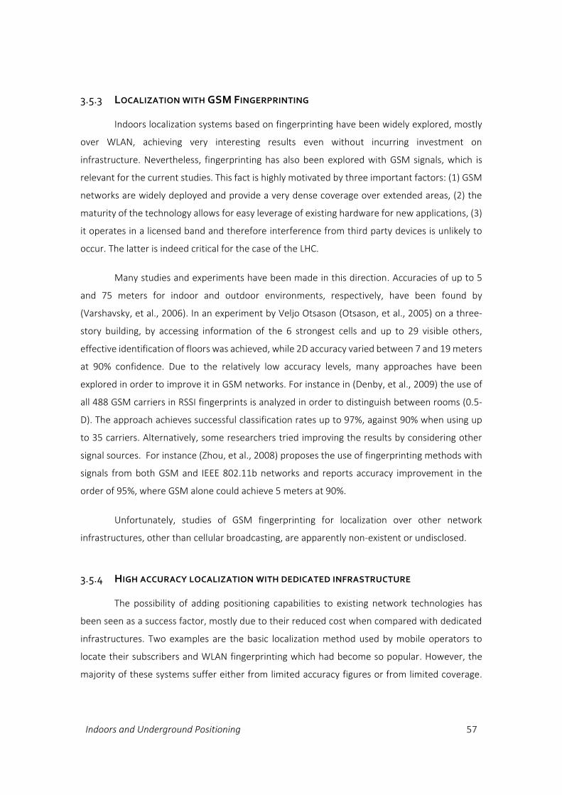
Indoors and Underground Positioning 57
3.5.3 LOCALIZATION WITH GSM FINGERPRINTING
Indoors localization systems based on fingerprinting have been widely explored, mostly
over WLAN, achieving very interesting results even without incurring investment on
infrastructure. Nevertheless, fingerprinting has also been explored with GSM signals, which is
relevant for the current studies. This fact is highly motivated by three important factors: (1) GSM
networks are widely deployed and provide a very dense coverage over extended areas, (2) the
maturity of the technology allows for easy leverage of existing hardware for new applications, (3)
it operates in a licensed band and therefore interference from third party devices is unlikely to
occur. The latter is indeed critical for the case of the LHC.
Many studies and experiments have been made in this direction. Accuracies of up to 5
and 75 meters for indoor and outdoor environments, respectively, have been found by
(Varshavsky, et al., 2006). In an experiment by Veljo Otsason (Otsason, et al., 2005) on a three-
story building, by accessing information of the 6 strongest cells and up to 29 visible others,
effective identification of floors was achieved, while 2D accuracy varied between 7 and 19 meters
at 90% confidence. Due to the relatively low accuracy levels, many approaches have been
explored in order to improve it in GSM networks. For instance in (Denby, et al., 2009) the use of
all 488 GSM carriers in RSSI fingerprints is analyzed in order to distinguish between rooms (0.5-
D). The approach achieves successful classification rates up to 97%, against 90% when using up
to 35 carriers. Alternatively, some researchers tried improving the results by considering other
signal sources. For instance (Zhou, et al., 2008) proposes the use of fingerprinting methods with
signals from both GSM and IEEE 802.11b networks and reports accuracy improvement in the
order of 95%, where GSM alone could achieve 5 meters at 90%.
Unfortunately, studies of GSM fingerprinting for localization over other network
infrastructures, other than cellular broadcasting, are apparently non-existent or undisclosed.
3.5.4 HIGH ACCURACY LOCALIZATION WITH DEDICATED INFRASTRUCTURE
The possibility of adding positioning capabilities to existing network technologies has
been seen as a success factor, mostly due to their reduced cost when compared with dedicated
infrastructures. Two examples are the basic localization method used by mobile operators to
locate their subscribers and WLAN fingerprinting which had become so popular. However, the
majority of these systems suffer either from limited accuracy figures or from limited coverage.
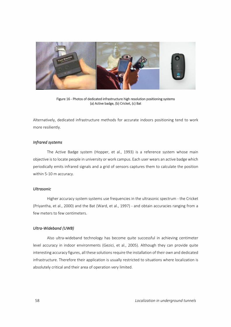
58 Localization in underground tunnels
Alternatively, dedicated infrastructure methods for accurate indoors positioning tend to work
more resiliently.
Infrared systems
The Active Badge system (Hopper, et al., 1993) is a reference system whose main
objective is to locate people in university or work campus. Each user wears an active badge which
periodically emits infrared signals and a grid of sensors captures them to calculate the position
within 5-10 m accuracy.
Ultrasonic
Higher accuracy system systems use frequencies in the ultrasonic spectrum - the Cricket
(Priyantha, et al., 2000) and the Bat (Ward, et al., 1997) - and obtain accuracies ranging from a
few meters to few centimeters.
Ultra-Wideband (UWB)
Also ultra-wideband technology has become quite successful in achieving centimeter
level accuracy in indoor environments (Gezici, et al., 2005). Although they can provide quite
interesting accuracy figures, all these solutions require the installation of their own and dedicated
infrastructure. Therefore their application is usually restricted to situations where localization is
absolutely critical and their area of operation very limited.
Figure 16 - Photos of dedicated infrastructure high resolution positioning systems (a) Active badge, (b) Cricket, (c) Bat
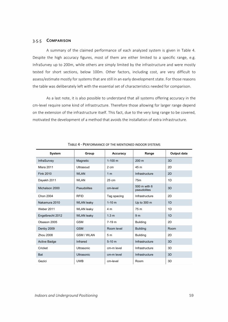
Indoors and Underground Positioning 59
3.5.5 COMPARISON
A summary of the claimed performance of each analyzed system is given in Table 4.
Despite the high accuracy figures, most of them are either limited to a specific range, e.g.
InfraSurvey up to 200m, while others are simply limited by the infrastructure and were mostly
tested for short sections, below 100m. Other factors, including cost, are very difficult to
assess/estimate mostly for systems that are still in an early development state. For those reasons
the table was deliberately left with the essential set of characteristics needed for comparison.
As a last note, it is also possible to understand that all systems offering accuracy in the
cm-level require some kind of infrastructure. Therefore those allowing for larger range depend
on the extension of the infrastructure itself. This fact, due to the very long range to be covered,
motivated the development of a method that avoids the installation of extra infrastructure.
TABLE 4 - PERFORMANCE OF THE MENTIONED INDOOR SYSTEMS
System Group Accuracy Range Output data
InfraSurvey Magnetic 1-100 m 200 m 3D
Misra 2011 Ultrasoud 2 cm 45 m 2D
Fink 2010 WLAN 1 m Infrastructure 2D
Dayekh 2011 WLAN 25 cm 75m 1D
Michalson 2000 Pseudolites cm-level 500 m with 6 pseudolites
3D
Chon 2004 RFID Tag spacing Infrastructure 2D
Nakamura 2010 WLAN leaky 1-10 m Up to 300 m 1D
Weber 2011 WLAN leaky 4 m 75 m 1D
Engelbrecht 2012 WLAN leaky 1.3 m 9 m 1D
Otsason 2005 GSM 7-19 m Building 2D
Denby 2009 GSM Room level Building Room
Zhou 2008 GSM / WLAN 5 m Building 2D
Active Badge Infrared 5-10 m Infrastructure 3D
Cricket Ultrasonic cm-m level Infrastructure 3D
Bat Ultrasonic cm-m level Infrastructure 3D
Gezici UWB cm-level Room 3D
60 Localization in underground tunnels
3.6 SUMMARY
This chapter focused on localization specifically for indoors and underground
environments. It starts by discussing the applications of indoors positioning, followed by a
characterization of the existing indoor localization technologies according to the signal type.
On a next section, an analysis of the requirements specific to underground tunnels is
performed, and they are compared to those typical indoors. Additionally, a characterization of
the requirements for localization in the LHC tunnel is also provided for the first time, where is it
clear that the project has very specific constraints and objectives, and therefore a new system
must be designed. Section 3.4 then characterizes the three different approaches for underground
signal transmission: Through-the- Air, Wire and Earth (TTA, TTW, and TTE respectively). A very
significant approach in TTW is the use of slotted shield leaky coaxial cable, or simply leaky-feeders,
as they enable dense and wide coverage of long hauls due to their relatively low attenuation.
These cables are present in the current tunnel setup and are exploited for localization purposes.
In the last section of the chapter a number of state-of-the-art studies and technologies
are mentioned which are relevant for the current PhD work. Among them there are works on
localization for underground mines, systems working over leaky-feeder, analyses of fingerprinting
with GSM networks and high-accuracy systems with dedicated infrastructure.
As understood by the comparison, there is no single system alone which can enable
localization over a wide range without starting to lose accuracy. A good example is the InfraSurvey
system, which claims accuracies in the order of 1% of the distance between emitter and receivers.
The exception to that rule are systems whose infrastructure is extensible by nature, like RFID,
WLAN or other beacon networks. However, deploying a dense network of beacons/tags over an
extended area might become cost prohibitive. In order to meet the localization requirements in
an area as long as the existing accelerator tunnels, this work investigates the approach of using
the existing leaky-feeder network without modifications for localization, with eventual
improvements for specific areas. The evaluation of the performance of such approach is
presented in the next chapters.
RSSI Characterization of Tunnel Networks over Leaky-Feeder cable 61
Chapter 4
RSSI CHARACTERIZATION OF TUNNEL
NETWORKS OVER LEAKY-FEEDER CABLE
The CERN accelerator tunnels and experimental halls present a unique scenario regarding
localization, offering interesting opportunities but imposing challenging requirements. This
chapter presents an in-depth analysis of the power profile observed for the GSM network
deployed over leaky feeder cable in the tunnel, for various conditions and scenarios. Tests with
WLAN are performed as well. The results provide valuable insight on the current environment
characteristics regarding the propagation and stability of electromagnetic signals, which has a
direct impact on the localization solutions.
4.1 RSSI FINGERPRINTING IN THE LHC
Many parameters were analyzed when selecting technologies for localization in the CERN
LHC. Besides the technical difficulties the medium presents by itself and the risks of interference,
the high levels of radiation present in the LHC invalidate any solution requiring installation of local
hardware.
4.1.1 MOTIVATION FOR FINGERPRINTING WITH GSM OVER LEAKY-FEEDER
During operation periods, the LHC machine accelerates particles to very high energy and
therefore the tunnel is classified as a high radiation area and made non-accessible. Due to the
radiation levels, non-specialized hardware would fail after some days of LHC operation and
sensitive devices like radio transceivers are definitely among the most affected classes of
electronics. In line with the existing technical solution for tunnel communication, the existence
of a network deployed over leaky-feeder was found to be an interesting opportunity to overcome

62 Localization in underground tunnels
that limitation. It provides wide coverage in the tunnels and is very reliable. Therefore, this
medium was taken into consideration for the design of the localization solution.
Among indoor location techniques, those based in the Received Signal Strength Indicator
(RSSI) are of particular interest since they require neither the installation of extra infrastructure
hardware nor allocation of extra spectrum. Besides the simplicity, RSSI methods do not require
additional emitters therefore eliminating the risk of interference.
RSSI fingerprinting shows up as attractive as challenging. Although this is effectively a 1-
D localization problem - as only one coordinate axis (along the tunnel) is required – the
differences to other indoor scenarios are notable and they might introduce serious issues. On the
one hand, localization is to be available along all tunnel’s length, i.e. nearly 27 km, which besides
possessing quite different shape from office and other spaces, is much beyond the length of any
other studied indoors location system or experiment. On the other hand, it is limited to the
existing network infrastructure. In the LHC the only network available throughout the tunnel is
GSM providing typically two channels per sector.
4.1.2 EXPERIMENTS WORKFLOW
To evaluate the applicability and performance of RSSI fingerprinting methods over the
leaky-feeder in the LHC tunnel, a series of experiments were conducted. Due to machine
Figure 17 - Tests methodology cycle

RSSI Characterization of Tunnel Networks over Leaky-Feeder cable 63
operation, data collection was only possible during short-time maintenance periods. Tests and
collection tools had to be prepared beforehand and sequent phases of analysis were taking place,
to extract conclusions and steer the next tests to be performed. The execution of these activities
has therefore been made in a cyclic fashion, where each iteration is delimited by a measurements
session in the tunnel, as suggested by Figure 17. Since some experiments were conducted several
times at different times, several data sets were collected. These explain the presence of several
sessions in the data presented in the next sections.
The first series of the experiments characterize the RSSI profile in the tunnel in several
different scenarios, for GSM and then WLAN networks. In a second series, presented in Chapter
5, this evaluation is performed in real-world conditions, where some localization algorithms are
tested and benchmarked against a radio-map built from the collected RSSI data.
4.2 CHARACTERIZATION OF THE GSM RSSI PROFILE
The experiments were conducted in a sector of the LHC comprising both straight and
bending sections. With the help of mobile phones, thousands of GSM RSSI samples were collected
to characterize the network and create the radio-maps.
4.2.1 LEAKY-FEEDERS NETWORK
GSM network coverage is available all along the tunnel’s length via a set of leaky-feeder
cables installed at nearly 2 m from the ground. For each tunnel section, two radio channels with
distinct radio signals are injected at each cable’s ends, therefore creating two GSM cells. Referring
to Figure 18, one can see the micro Base Stations (represented as red squares) and the
coupling/amplification points of the signal into the leaky-feeder (as pink arrows). Besides the GSM
network, also an emergency VHF network was carried along which is now being replaced by
TETRA.
As a consequence of this configuration, as one goes along the tunnel, one of the radio
channels gets stronger while the other attenuates (Pereira, et al., 2011). According to the vendor
specifications (RFS World, 2010), the cable is specially designed for tunnels, providing low
coupling loss variations. It propagates electromagnetic waves of up to 1950 MHz and it exhibits a
longitudinal loss of 3.16 dB/100m at 900 MHz.

64 Localization in underground tunnels
4.2.2 EXPERIMENTS SETUP
In an initial phase, to characterize the network signal strength profile, several types of
measurements were carried out. However, in GSM networks, terminals can only be associated to
a single cell and, except for specific vendor solutions, information about the neighbor cells is not
directly accessible through the terminals’ APIs. Nevertheless, they continuously monitor the
conditions of adjacent cells so that the network can perform informed handovers and maintain
the channel quality as high as possible. Furthermore several aforementioned studies indeed
made use of the neighbor cells’ information to increase the performance of fingerprinting
methods. In order to continuously monitor and store the signal strength of the network a custom
device was setup.
In our tests we used Nokia 6150 mobile phones in which we enabled the NetMonitor
menus (see Figure 19). These additional pages of information allowed us to individually acquire
the signal strength of the 6 strongest cells, which was updated nearly every second. All
fingerprints were automatically recorded to a laptop running a capture and parsing software
taking advantage of the Gammu utility (Čihař, online). Three of these terminals were used in
parallel, controlled simultaneously by a custom fingerprint collection software. This configuration
Figure 18 - GSM frequencies along the tunnel. The pink arrows represent the injection points of GSM frequencies
RSSI Characterization of Tunnel Networks over Leaky-Feeder cable 65
enabled the collection of triple the amount of fingerprints in the same time frame and provided
valuable hints on the signal changes on a short spatial scale.
Among the performed experiments, the following are of particular interest:
Detailed longitudinal measurements, with fingerprints taken every 40 meters in a section
of 600 m and 10 samples per fingerprint. Four of such sessions were carried out.
Fine-grained longitudinal measurements, where the signal strength was acquired every 10
meters for a section of 280 meters, using two terminals simultaneously. 30 samples
were collected for each fingerprint and two sessions were carried out.
Fixed location measurements, where 150 samples of the signal strength were collected at
the same position to account for variations depending on the measurement conditions.
Radial measurements, with fingerprints taken every 10 cm for a distance of 1.10 m
between the wall and the LHC machine, at 50cm from the ground, 1000 samples per
fingerprint. Three devices were used in parallel for data collection.
After characterizing the RSSI profile of the GSM network, a longitudinal assessment of
the RSSI evolution for WLAN 802.11 was also performed, which allows us to compare and draw
some conclusions on the differences.
Figure 19 - Equipment used for data collection

66 Localization in underground tunnels
4.2.3 RSSI ACCORDING TO POSITION
Among the most important characteristics of the Leaky-feeder cable is its low longitudinal
attenuation. Therefore two experiments on assessing the RSSI along the cable were performed,
having different step sizes: 40m and 10m.
In the first set of measurements (Pereira, et al., 2011), as we go along the tunnel we
notice that the received signal strength can change significantly. In Figure 20, the mean and
standard deviation of the RSSI values are shown as a function of the distance for the two most
indicative sessions. We can clearly see two dominant GSM channels and traces of several
channels from nearby tunnel sections. In the plot we can also identify two distinct areas,
specifically before and after 240 m. In fact, the leaky-feeder is injected a new GSM channel at this
location. Until then the new frequency experiences high attenuation as it propagates through air.
After that point the propagation occurs normally in the cable and, therefore, the attenuation is
much lower. In this region, approximating the RSSI evolution to a linear function, we obtained
Figure 20 - RSSI evolution along the tunnel in a section of 600 m Fingerprints were taken at every 40m. Each color represents a different channel, error bars represent
standard deviation and shaded areas are delimited by the minimum and maximum RSSI values of the same frequency, obtained in different measurements sessions.
RSSI Characterization of Tunnel Networks over Leaky-Feeder cable 67
attenuation factors of 3.9 and 4.5 dB/km, slightly larger than the attenuation of the cable as in its
specification.
Despite the fact that the cable’s longitudinal attenuation introduces measurable signal
changes, the variations in the RSSI values tend to obfuscate them. These effects are generally
caused by the volatility of the measurement conditions but are also due to the influence of
multipath propagation in the tunnel and multicoupling in the leaky-feeder itself (Weber, et al.,
2010).
In order to better assess this effect, measurements were performed with a significantly
smaller step, 10 meters, in a nearby region of the tunnel (Pereira, et al., 2012). Figure 21 presents
the result of such measurements, as captured by two mobiles simultaneously, and shows many
interesting aspects. In the first place one can notice that, in this region, a third channel can be
observed and its RSSI well characterized. This fact shows that in some regions of the tunnel, the
interconnections of the leaky feeder actually allow the nearby signal to pass through, creating a
third usable GSM channel. Although not very strong, the additional channel is, where available,
certainly an additional valuable resource for RSSI fingerprinting. Another very important point is
that, even though two terminals were used per session and installed less than 10 cm apart, the
RSSI values assessed by them always exhibit some discrepancy, to the point that, looking at the
plot, it is not possible to say which two RSSI lines belong to the same session. From this
observation we can conclude that the exact position of the receivers greatly influences its
captured RSSI. Furthermore such discrepancies are mostly independent for each channel.
4.2.4 INTER-CHANNEL RSSI DIFFERENTIAL
In a network configuration like the one presented, several channels propagate over a
leaky-feeder cable. Along these cables the various channels suffer a certain level of attenuation,
depending on the cable characteristics, the distance travelled by the signal and the signal’s
frequency. This property normally characterized for each cable in terms of an attenuation
coefficient stated in dB/100m for a given set of frequencies. Assuming the factor is constant all
along the cable, the same level of attenuation should be found in all the channels when moving
from one position to another. Even though the measurement conditions are likely to change
slightly (for instance due to self-shadowing of the person conducting the measurement, changing
body postures, different configuration and operational state of the accelerator equipment, etc…)
they would affect the channels the same way. In this scenario if two channels were injected from
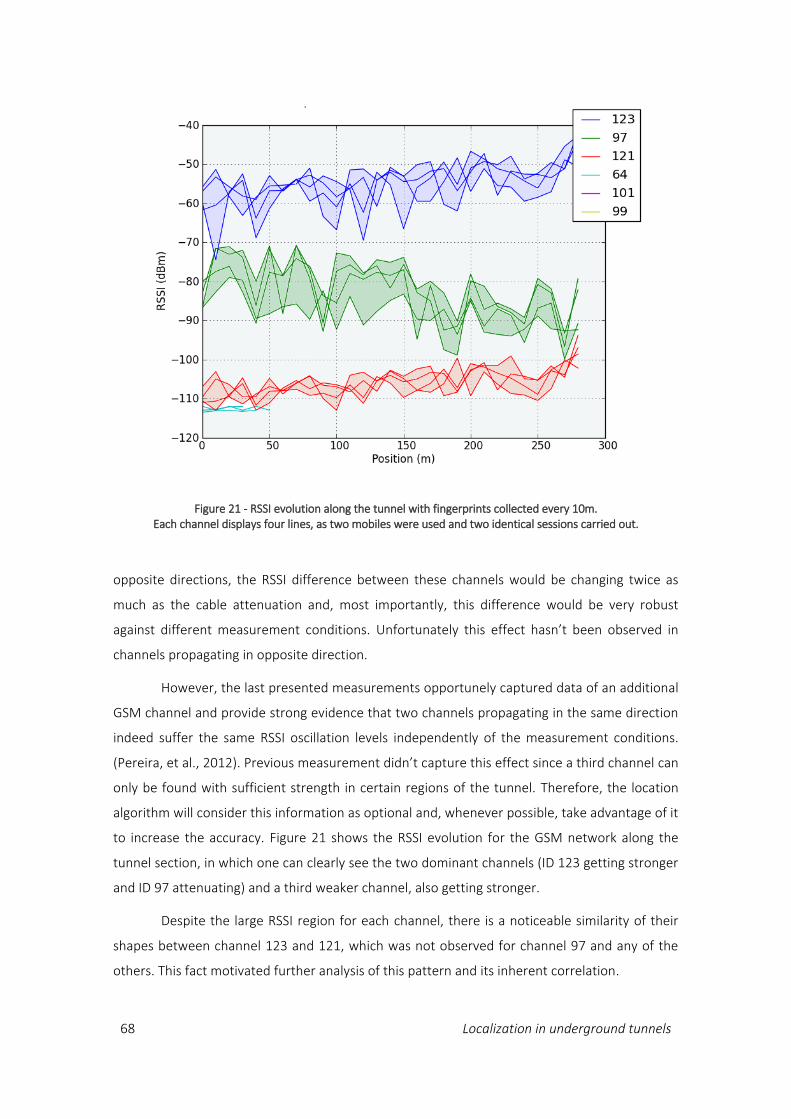
68 Localization in underground tunnels
opposite directions, the RSSI difference between these channels would be changing twice as
much as the cable attenuation and, most importantly, this difference would be very robust
against different measurement conditions. Unfortunately this effect hasn’t been observed in
channels propagating in opposite direction.
However, the last presented measurements opportunely captured data of an additional
GSM channel and provide strong evidence that two channels propagating in the same direction
indeed suffer the same RSSI oscillation levels independently of the measurement conditions.
(Pereira, et al., 2012). Previous measurement didn’t capture this effect since a third channel can
only be found with sufficient strength in certain regions of the tunnel. Therefore, the location
algorithm will consider this information as optional and, whenever possible, take advantage of it
to increase the accuracy. Figure 21 shows the RSSI evolution for the GSM network along the
tunnel section, in which one can clearly see the two dominant channels (ID 123 getting stronger
and ID 97 attenuating) and a third weaker channel, also getting stronger.
Despite the large RSSI region for each channel, there is a noticeable similarity of their
shapes between channel 123 and 121, which was not observed for channel 97 and any of the
others. This fact motivated further analysis of this pattern and its inherent correlation.
Figure 21 - RSSI evolution along the tunnel with fingerprints collected every 10m. Each channel displays four lines, as two mobiles were used and two identical sessions carried out.
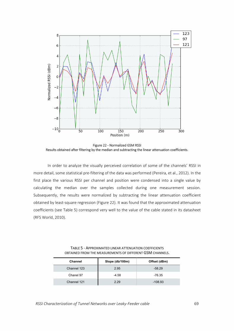
RSSI Characterization of Tunnel Networks over Leaky-Feeder cable 69
In order to analyze the visually perceived correlation of some of the channels’ RSSI in
more detail, some statistical pre-filtering of the data was performed (Pereira, et al., 2012). In the
first place the various RSSI per channel and position were condensed into a single value by
calculating the median over the samples collected during one measurement session.
Subsequently, the results were normalized by subtracting the linear attenuation coefficient
obtained by least-square regression (Figure 22). It was found that the approximated attenuation
coefficients (see Table 5) correspond very well to the value of the cable stated in its datasheet
(RFS World, 2010).
Figure 22 - Normalized GSM RSSI Results obtained after filtering by the median and subtracting the linear attenuation coefficients.
TABLE 5 - APPROXIMATED LINEAR ATTENUATION COEFFICIENTS OBTAINED FROM THE MEASUREMENTS OF DIFFERENT GSM CHANNELS.
Channel Slope (db/100m) Offset (dBm)
Channel 123 2.95 -58.29
Chanel 97 -4.58 -76.35
Channel 121 2.29 -108.93

70 Localization in underground tunnels
Finally Spearman’s rank order coefficient and the Root mean squared deviation were
used to quantify the actual level of similarity. The correlation among the channels has been
studied for each measurement session individually as shown in Table 6.
As can be seen, significant correlation exists generally between the channels 121 & 123,
whereas lower dependence and larger deviations can be observed between the channels 97 &
123. The correlation is even more noticeable if the data of the different measurement sessions
are not considered individually but combined - Figure 22 - which yields a Spearman rank-order
coefficient of 0.99 and a root-mean square deviation of 0.92.
Therefore, the RSSI differential of these channels can be considered as a quite robust
characteristic of a given location, which might then be leveraged for location finding. Hereafter,
this measure is designated as the Inter Channel RSSI Differential (ICRD), which for the case of two
channels whose signal propagates in the same direction, is defined as Same-Propagation-
Direction ICRD (SPD-ICRD).
4.2.5 RSSI DEPENDENCE UPON MEASUREMENT CONDITIONS
Although the four detailed measurement sessions were performed in rather similar
conditions, the observed RSSI values at each point exhibit divergent behaviors. It was interesting
how one can have almost null variance in two consecutive measurements while their average
differs by more than 10 dB (e.g.: measurement at 480m in Figure 20).
This fact motivated the stationary measurements (Pereira, et al., 2011) in where we
tested three slightly different conditions:
TABLE 6 - CORRELATION COEFFICIENTS AMONG THE CHANNELS CALCULATED PER MEASUREMENT SESSION AND MOBILE
Correlation coefficients per session Spearman rank-order coefficient Root-mean sq. deviation
Channels 123 & 121
Session 1.1 0.976 1.845
Session 1.2 0.978 1.755
Session 2.1 0.963 2.269
Session 2.2 0.971 1.951
Channels 123 & 97
Session 1.1 0.720 6.260
Session 1.2 0.689 6.601
Session 2.1 0.660 6.896
Session 2.2 0.848 4.586
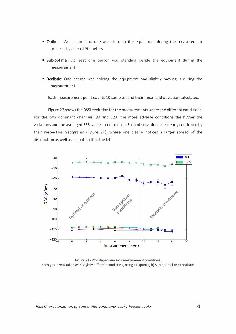
RSSI Characterization of Tunnel Networks over Leaky-Feeder cable 71
Optimal: We ensured no one was close to the equipment during the measurement
process, by at least 30 meters.
Sub-optimal: At least one person was standing beside the equipment during the
measurement
Realistic: One person was holding the equipment and slightly moving it during the
measurement.
Each measurement point counts 10 samples, and their mean and deviation calculated.
Figure 23 shows the RSSI evolution for the measurements under the different conditions.
For the two dominant channels, 80 and 123, the more adverse conditions the higher the
variations and the averaged RSSI values tend to drop. Such observations are clearly confirmed by
their respective histograms (Figure 24), where one clearly notices a larger spread of the
distribution as well as a small shift to the left.
Figure 23 - RSSI dependence on measurement conditions. Each group was taken with slightly different conditions, being a) Optimal, b) Sub-optimal or c) Realistic.
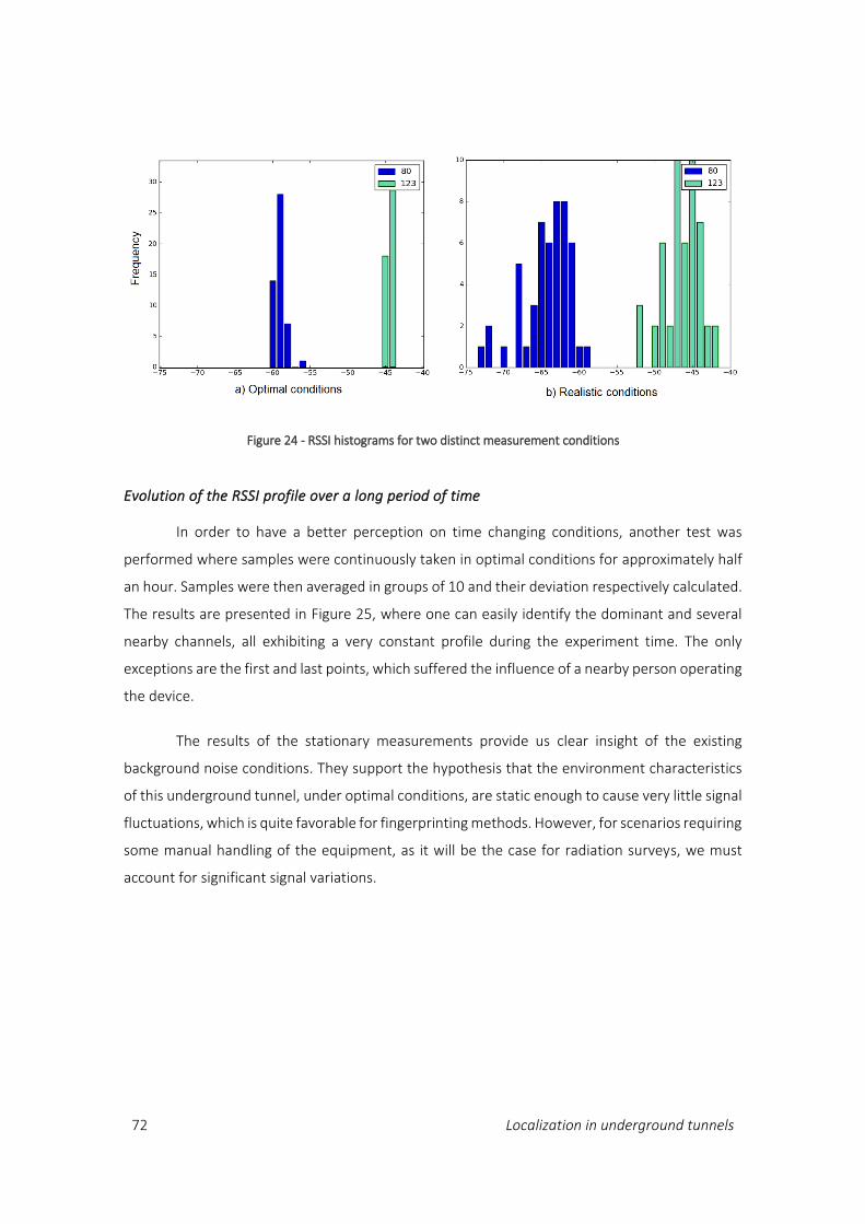
72 Localization in underground tunnels
Evolution of the RSSI profile over a long period of time
In order to have a better perception on time changing conditions, another test was
performed where samples were continuously taken in optimal conditions for approximately half
an hour. Samples were then averaged in groups of 10 and their deviation respectively calculated.
The results are presented in Figure 25, where one can easily identify the dominant and several
nearby channels, all exhibiting a very constant profile during the experiment time. The only
exceptions are the first and last points, which suffered the influence of a nearby person operating
the device.
The results of the stationary measurements provide us clear insight of the existing
background noise conditions. They support the hypothesis that the environment characteristics
of this underground tunnel, under optimal conditions, are static enough to cause very little signal
fluctuations, which is quite favorable for fingerprinting methods. However, for scenarios requiring
some manual handling of the equipment, as it will be the case for radiation surveys, we must
account for significant signal variations.
Figure 24 - RSSI histograms for two distinct measurement conditions

RSSI Characterization of Tunnel Networks over Leaky-Feeder cable 73
4.2.6 RADIAL MEASUREMENTS
According to some studies available in the literature, even though the RSSI is more stable
using Leaky-Feeder cables than with regular access points, significant signal variations occur due
to fast fading and eventual presence of obstacles. To better account for these effects in the
underground GSM network, a set of samples was taken in the same longitudinal position but
slightly changing the distance to the cable, as specified in section 4.2.2.
Having a step of 10 cm, the attenuation due to space propagation can be considered as
negligible. The RSSI variations therefore depend mostly on the fast-fading and self-coupling
effects, and the results are very expressive, as shown in Figure 26.
Even though the RSSI values at each measured point were quite constant over time (note
that the standard deviation bars for each point are almost invisible), they showed significant
dependence on small scale location changes. If one considers all the measurements for each
device and channel, i.e., each line in the plot, the overall distribution is found to be quite large.
Figure 25 - RSSI profile evaluated for a period of nearly 30 minutes. Both the dominant and detected nearby channels RSSIs are kept very constant over time.
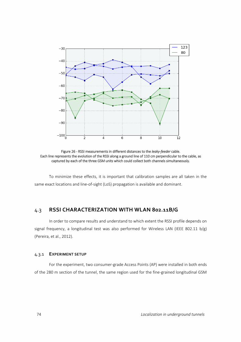
74 Localization in underground tunnels
To minimize these effects, it is important that calibration samples are all taken in the
same exact locations and line-of-sight (LoS) propagation is available and dominant.
4.3 RSSI CHARACTERIZATION WITH WLAN 802.11B/G
In order to compare results and understand to which extent the RSSI profile depends on
signal frequency, a longitudinal test was also performed for Wireless LAN (IEEE 802.11 b/g)
(Pereira, et al., 2012).
4.3.1 EXPERIMENT SETUP
For the experiment, two consumer-grade Access Points (AP) were installed in both ends
of the 280 m section of the tunnel, the same region used for the fine-grained longitudinal GSM
Figure 26 - RSSI measurements in different distances to the leaky-feeder cable. Each line represents the evolution of the RSSI along a ground line of 110 cm perpendicular to the cable, as
captured by each of the three GSM units which could collect both channels simultaneously.

RSSI Characterization of Tunnel Networks over Leaky-Feeder cable 75
measurements. Each AP is based on the Realtek 8187L chipset equipped with a high-gain (9 dBi)
omnidirectional antenna. As illustrated by Figure 27, the APs were installed 150 m from each
other and their antennas placed in parallel to the leaky feeder at a distance between 5 and 10
cm. This configuration promoted the injection and propagation of WLAN signal through the cable
instead of direct connection. Furthermore, LOS conditions between the transmitters and the
receiver unit were reduced by installing a reflexive shield, made out aluminum foil, near the APs.
Four measurement sessions were executed, in which the RSSI fingerprints were collected
at identical positions as those from GSM, every 10 m, each one counting 100 samples.
Each AP provided its own channel, being used channel 1 (2.412 GHz) and 9 (2.452 GHz)
on the left and right APs respectively. They were programmed to send beacon frames every 30
ms, which were then captured, parsed and stored by a mobile unit in common RSSI database.
This configuration also allowed for the subsequent processing of the data by the different
algorithms, independently of the data-source.
Figure 27 - WLAN experiment setup. The shields avoid LoS conditions and the position of the antennas promote
signal injection in the leaky-feeder cable.
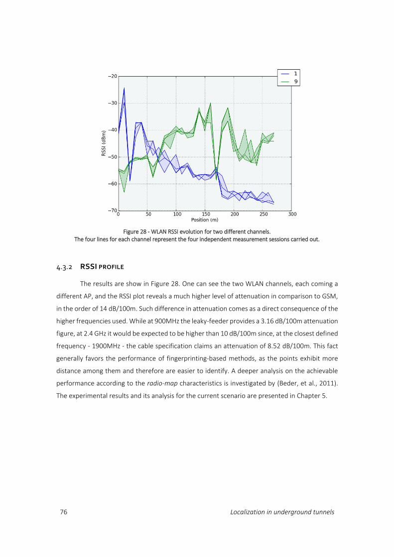
76 Localization in underground tunnels
4.3.2 RSSI PROFILE
The results are show in Figure 28. One can see the two WLAN channels, each coming a
different AP, and the RSSI plot reveals a much higher level of attenuation in comparison to GSM,
in the order of 14 dB/100m. Such difference in attenuation comes as a direct consequence of the
higher frequencies used. While at 900MHz the leaky-feeder provides a 3.16 dB/100m attenuation
figure, at 2.4 GHz it would be expected to be higher than 10 dB/100m since, at the closest defined
frequency - 1900MHz - the cable specification claims an attenuation of 8.52 dB/100m. This fact
generally favors the performance of fingerprinting-based methods, as the points exhibit more
distance among them and therefore are easier to identify. A deeper analysis on the achievable
performance according to the radio-map characteristics is investigated by (Beder, et al., 2011).
The experimental results and its analysis for the current scenario are presented in Chapter 5.
Figure 28 - WLAN RSSI evolution for two different channels.
The four lines for each channel represent the four independent measurement sessions carried out.
RSSI Characterization of Tunnel Networks over Leaky-Feeder cable 77
4.4 CONCLUSIONS
The characterization of the GSM and WLAN signals’ power in the tunnel is an essential
step in understanding, in the first place, the opportunities and challenges for fingerprinting
techniques with RSSI measurements. In a network configuration as presented, where the signal
propagates through leaky-feeder cable, the attenuation of the power is expected to be
considerably lower than in the case of free-space-loss communication.
By analyzing the RSSI profile of the existing GSM network, it was found that the measured
longitudinal attenuation ratios conform to the specification of the cable, i.e., in the order of 3
dB/100m. Nevertheless, at such low attenuation factors, the small power disturbances and
fluctuations due to fast-fading, reflections and obstacles (including the measurement device
itself), found to be up to 10 dB, can easily obfuscate the signal attenuation introduced by the
cable. From this fact one can draw the conclusion that RSSI localization with resource to analytical
methods is very limited. Indeed, according to the free-space model, distance errors would be
proportional to the ratio between the RSSI fluctuations and the cable’s attenuation, i.e., in the
order of 300 meters.
In turn, being an empirical method, fingerprinting can explore other properties of the
measurements for uniqueness search and location matching. For that a more detailed scan was
performed and a third GSM channel was found. Since two of those channels had follow the same
propagation direction, their pattern was further analyzed and interestingly found to very similar
among them, up to a 99% spearman rank-order coefficient. From this observation, the same-
propagation-direction inter-channel RSSI differential (SPD-ICRD) seems fairly resilient to signal
power disturbances and fluctuations.
However fingerprinting methods are also bound to the validity of the radio-map, which
can be assessed with the reproducibility of the measurements. In order to evaluate that, several
sessions, accounting for similar and slightly different measurement conditions, were performed.
From the longitudinal measurements, where several collection sessions were carried out under
similar conditions, one can see that some significant differences arise at some points – see for
instance the region of channel 97 in Figure 21. This fact raised the interest on what could be
affecting the RSSI to that extent. Therefore further tests were conducted analyzing the effects of
the measurement conditions and differences in the distance to the cable. The results are very
expressive, showing that these factors have a very strong impact on the measurements: under
realistic conditions, where the measurement device is moved slowly by a person operating it, a
78 Localization in underground tunnels
much larger RSSI distribution appears and the mean value drops by 2 to 4 dB’s; additionally, when
slightly moving the measurement device away from the leaky-feeder, the RSSI variations are very
considerable, exhibiting deltas of more than 20 dB’s.
The tests characterizing the GSM signal on the LHC tunnel deployed over leaky-feeder
cable provide a very good insight on the power variation according to the longitudinal position,
but also on its behavior when subject to different measurement conditions and distance to cable.
It is experimentally shown that, although the longitudinal attenuation stays within the cable
specification, the signals’ RSSI is heavily affected when testing for the change of conditions.
Although the reason behind such acute sensitivity is not completely understood, we do believe
that the metallic outer shell of the magnets and the presence of large metallic information panels
on the walls and on the magnets’ shells highly contribute to the creation of complex reflection
fields, exhibiting non-uniform power patterns. Unfortunately a detailed study of these conditions
would require changes to the current environment which are not possible.
Furthermore, in order to check for technology dependence, experiments with WLAN
were carried out in which two AP’s create two channels and promote their propagation over the
leaky-feeder cable. The experiments shows that a much higher attenuation occurs longitudinally,
in the order of 14 dB/100m, and that differences arising among independent measurement
sessions are much narrower than in GSM, usually lower than 3 dB’s. This fact further emphasizes
that GSM frequencies are especially more sensitive to interference and, therefore, their
performance with fingerprinting for location purposes may reasonably be inferior.
Proposed RSSI Fingerprinting Methods and Performance Evaluation 79
Chapter 5
PROPOSED RSSI FINGERPRINTING METHODS
AND PERFORMANCE EVALUATION
After the characterization of the RSSI profile in the tunnel, an additional phase was taken
for the development and test of new fingerprinting algorithms, taking into account the observed
signal characteristics. We start by analyzing the raw performance of several distance metrics,
then a new distance metric is tested, and tests using GSM and WLAN are performed.
The performance is assessed via a new software utility which, using a dedicated set of
samples from the radio-map, computes the algorithms’ ranking and their accuracy level in
realistic conditions. In the last part of the chapter some considerations on the achieved
performance levels and their limits are provided.
5.1 EXPERIMENTS SETUP
In order to evaluate the performance of fingerprinting methods for the current
environment several points had to be addressed. First, it would be of utmost importance to make
the tests in realistic conditions, so that the measured performance levels could reflect those of
the real work scenario of radiation surveying. Second, it would be necessary to design and
implement a solution for automated test and benchmarking of the several location algorithms.
Only with such a tool the algorithms’ performance could be evaluated and compared among
them, and their modifications and respective parameter tuning could incur a smaller penalty time
due to the re-running of all the necessary tests. At last, it would be required to re-use some of
the collected data, both GSM and WLAN RSSI, and store it to a common database. In this database
data also had to be preprocessed, so that tests with large fingerprint count are (1) faster to
execute and (2) mimic the real conditions in the case of a full tunnel fingerprint database. The
experiment setup and the software tool implemented for the case are described next.
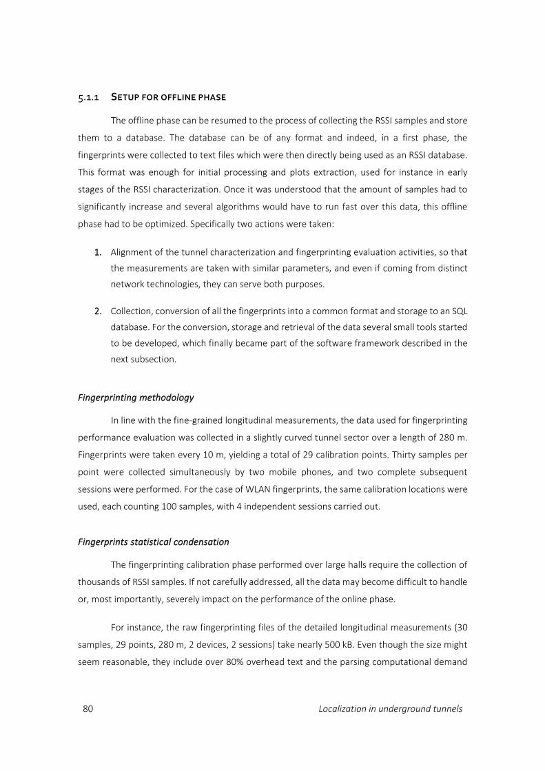
80 Localization in underground tunnels
5.1.1 SETUP FOR OFFLINE PHASE
The offline phase can be resumed to the process of collecting the RSSI samples and store
them to a database. The database can be of any format and indeed, in a first phase, the
fingerprints were collected to text files which were then directly being used as an RSSI database.
This format was enough for initial processing and plots extraction, used for instance in early
stages of the RSSI characterization. Once it was understood that the amount of samples had to
significantly increase and several algorithms would have to run fast over this data, this offline
phase had to be optimized. Specifically two actions were taken:
1. Alignment of the tunnel characterization and fingerprinting evaluation activities, so that
the measurements are taken with similar parameters, and even if coming from distinct
network technologies, they can serve both purposes.
2. Collection, conversion of all the fingerprints into a common format and storage to an SQL
database. For the conversion, storage and retrieval of the data several small tools started
to be developed, which finally became part of the software framework described in the
next subsection.
Fingerprinting methodology
In line with the fine-grained longitudinal measurements, the data used for fingerprinting
performance evaluation was collected in a slightly curved tunnel sector over a length of 280 m.
Fingerprints were taken every 10 m, yielding a total of 29 calibration points. Thirty samples per
point were collected simultaneously by two mobile phones, and two complete subsequent
sessions were performed. For the case of WLAN fingerprints, the same calibration locations were
used, each counting 100 samples, with 4 independent sessions carried out.
Fingerprints statistical condensation
The fingerprinting calibration phase performed over large halls require the collection of
thousands of RSSI samples. If not carefully addressed, all the data may become difficult to handle
or, most importantly, severely impact on the performance of the online phase.
For instance, the raw fingerprinting files of the detailed longitudinal measurements (30
samples, 29 points, 280 m, 2 devices, 2 sessions) take nearly 500 kB. Even though the size might
seem reasonable, they include over 80% overhead text and the parsing computational demand

Proposed RSSI Fingerprinting Methods and Performance Evaluation 81
to extract the useful data is very significant. Therefore it becomes unreasonable to use the raw
files directly for the online phase, when all the fingerprints are required at once.
To overcome this problem and considerably reducing the database size, all the samples
were processed per point and network technology and several statistical parameters describing
each fingerprint were calculated:
Minimum and maximum
Quartiles
Histogram, fenced at 1.5*Inter-Quartile Range (IQR) (Frigge, et al., 1989)
Histogram high and low fence
By saving the histogram fenced according to the IQR, one significantly reduces the
presence of outliers, while efficiently storing the samples RSSI information. Moreover, from these
entries one can very easily obtain other statistical measures, like the median which is also the
second quartile.
Since it is not common - and arguably worthless - for fingerprinting methods to operate
directly on all the samples, statistical information is stored into the fingerprinting database and
the RSSI samples optionally skipped. All the implemented online methods make use of statistical
information only.
Fingerprinting database format
An SQL fingerprinting database was designed and implemented in SQLite so that they
would be centralized and accessible in a standard way. Some additional tools were implemented
to parse and save the RSSI data into this repository. For each measurement session, 3 database
tables are created:
[calibration_id]_rssi - A table containing all the raw RSSI samples, and eventually other
information coming from the capture software, like channel noise estimation.
A typical GSM entry consists of the following fieds:
[Session, Mobile, Point, Channel], Sample, Power, C1, C2
The first four fields - identifying the fingerprint - and the Sample field - identifying the
sample number - are all integer, the Power, C1 and C2 fields are dB’s stored as “floats”.
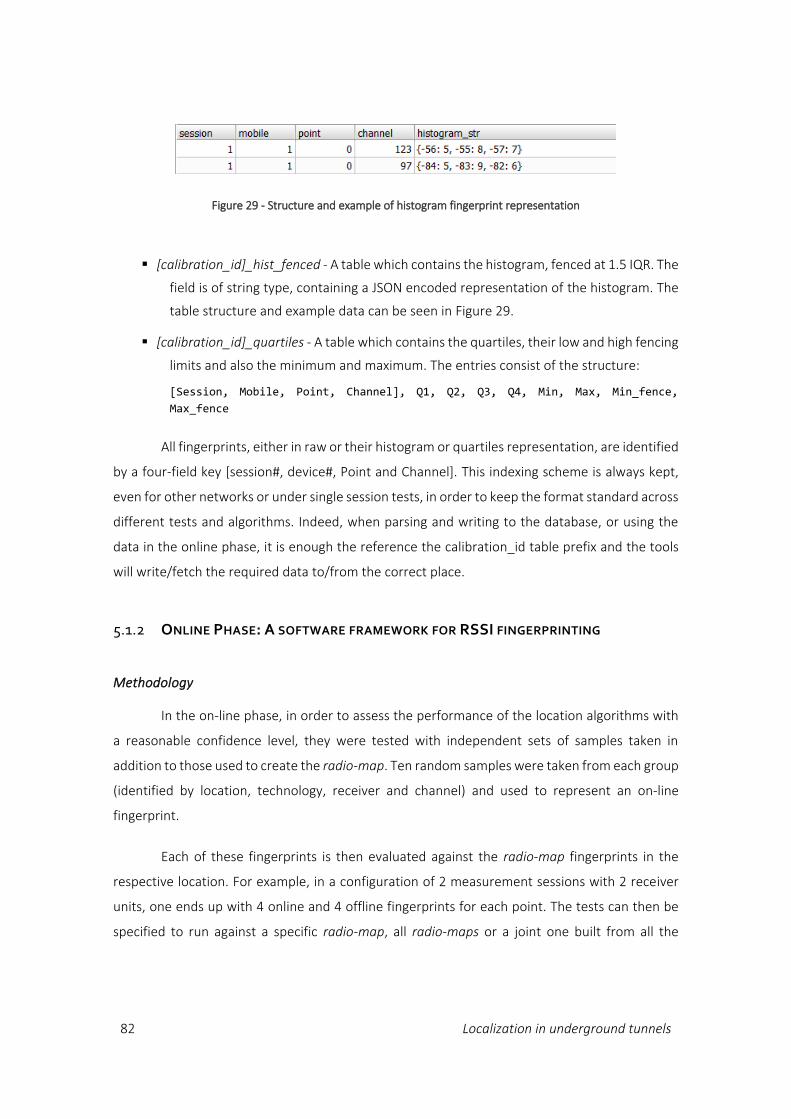
82 Localization in underground tunnels
[calibration_id]_hist_fenced - A table which contains the histogram, fenced at 1.5 IQR. The
field is of string type, containing a JSON encoded representation of the histogram. The
table structure and example data can be seen in Figure 29.
[calibration_id]_quartiles - A table which contains the quartiles, their low and high fencing
limits and also the minimum and maximum. The entries consist of the structure:
[Session, Mobile, Point, Channel], Q1, Q2, Q3, Q4, Min, Max, Min_fence,
Max_fence
All fingerprints, either in raw or their histogram or quartiles representation, are identified
by a four-field key [session#, device#, Point and Channel]. This indexing scheme is always kept,
even for other networks or under single session tests, in order to keep the format standard across
different tests and algorithms. Indeed, when parsing and writing to the database, or using the
data in the online phase, it is enough the reference the calibration_id table prefix and the tools
will write/fetch the required data to/from the correct place.
5.1.2 ONLINE PHASE: A SOFTWARE FRAMEWORK FOR RSSI FINGERPRINTING
Methodology
In the on-line phase, in order to assess the performance of the location algorithms with
a reasonable confidence level, they were tested with independent sets of samples taken in
addition to those used to create the radio-map. Ten random samples were taken from each group
(identified by location, technology, receiver and channel) and used to represent an on-line
fingerprint.
Each of these fingerprints is then evaluated against the radio-map fingerprints in the
respective location. For example, in a configuration of 2 measurement sessions with 2 receiver
units, one ends up with 4 online and 4 offline fingerprints for each point. The tests can then be
specified to run against a specific radio-map, all radio-maps or a joint one built from all the
Figure 29 - Structure and example of histogram fingerprint representation
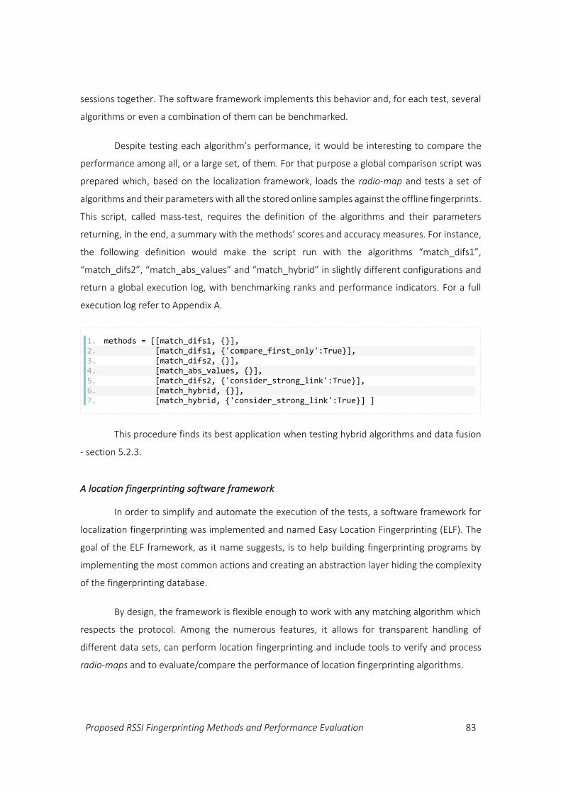
Proposed RSSI Fingerprinting Methods and Performance Evaluation 83
sessions together. The software framework implements this behavior and, for each test, several
algorithms or even a combination of them can be benchmarked.
Despite testing each algorithm’s performance, it would be interesting to compare the
performance among all, or a large set, of them. For that purpose a global comparison script was
prepared which, based on the localization framework, loads the radio-map and tests a set of
algorithms and their parameters with all the stored online samples against the offline fingerprints.
This script, called mass-test, requires the definition of the algorithms and their parameters
returning, in the end, a summary with the methods’ scores and accuracy measures. For instance,
the following definition would make the script run with the algorithms “match_difs1”,
“match_difs2”, “match_abs_values” and “match_hybrid” in slightly different configurations and
return a global execution log, with benchmarking ranks and performance indicators. For a full
execution log refer to Appendix A.
This procedure finds its best application when testing hybrid algorithms and data fusion
- section 5.2.3.
A location fingerprinting software framework
In order to simplify and automate the execution of the tests, a software framework for
localization fingerprinting was implemented and named Easy Location Fingerprinting (ELF). The
goal of the ELF framework, as it name suggests, is to help building fingerprinting programs by
implementing the most common actions and creating an abstraction layer hiding the complexity
of the fingerprinting database.
By design, the framework is flexible enough to work with any matching algorithm which
respects the protocol. Among the numerous features, it allows for transparent handling of
different data sets, can perform location fingerprinting and include tools to verify and process
radio-maps and to evaluate/compare the performance of location fingerprinting algorithms.
1. methods = [[match_difs1, {}], 2. [match_difs1, {'compare_first_only':True}], 3. [match_difs2, {}], 4. [match_abs_values, {}], 5. [match_difs2, {'consider_strong_link':True}], 6. [match_hybrid, {}], 7. [match_hybrid, {'consider_strong_link':True}] ]
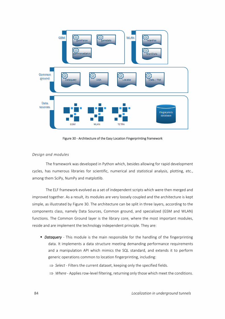
84 Localization in underground tunnels
Design and modules
The framework was developed in Python which, besides allowing for rapid development
cycles, has numerous libraries for scientific, numerical and statistical analysis, plotting, etc.,
among them SciPy, NumPy and matplotlib.
The ELF framework evolved as a set of independent scripts which were then merged and
improved together. As a result, its modules are very loosely coupled and the architecture is kept
simple, as illustrated by Figure 30. The architecture can be split in three layers, according to the
components class, namely Data Sources, Common ground, and specialized (GSM and WLAN)
functions. The Common Ground layer is the library core, where the most important modules,
reside and are implement the technology independent principle. They are:
Dataquery - This module is the main responsible for the handling of the fingerprinting
data. It implements a data structure meeting demanding performance requirements
and a manipulation API which mimics the SQL standard, and extends it to perform
generic operations common to location fingerprinting, including:
Select - Filters the current dataset, keeping only the specified fields.
Where - Applies row-level filtering, returning only those which meet the conditions.
Figure 30 - Architecture of the Easy Location Fingerprinting framework

Proposed RSSI Fingerprinting Methods and Performance Evaluation 85
Group_by - Like in SQL, it groups data having the same values in the selected fields
and reduces the groups to a single item using a specified function, like SUM.
Organize_by - It groups data having the same values in the selected fields, without
reducing. It can optionally create a nested data structure.
Get_group - It returns a group from a nested data structure, whose indexing field
values match those provided.
Flatten - It transforms a nested data structure into a flat one.
Combine - It allows for combining data from two sets which might be grouped,
eventually performing reduce binary operations, like difference, sum, etc.
Order_by - It orders a dataset by the specified fields, lowest to highest or reverse.
DBA - This module implements an abstraction layer to the fingerprints database. It is
responsible for the creation of the data tables given a dataset (import2db function),
importing the generated statistics (import_stats2db) and data fetching (table_select).
Data fetching with automatic table resolving is implemented in the Stats module, since
it is the only kind of information required by the location algorithms.
Locator - The locator is the central module implementing location fingerprinting functions
and defining the interface for integrating additional algorithms. This interface is
explained in the next part - Interoperation protocols. The locator modules includes the
several proposed location finding methods and their required pattern matching
algorithms, as well and evaluation routines for the algorithms - see “Approaches for
performance evaluation of location fingerprinting algorithms” and also a template
script for global testing. Among the implemented pattern matching algorithms,
available in this module, there is match_abs_values for matching fingerprints based on
their absolute RSSI, and match_difs for matching fingerprints based on their differential
RSSI (ICRD); a hybrid implementation (match_hybrid) and a customizable KNN
algorithm. The algorithms are explained in part 5.2.
Stats & Plotting - Functions related to the statistical analysis of the fingerprinting data,
allowing to (1) generate the required statistics from the raw RSSI values and store them
in the database, (2) apply statistical transformations to a dataset, including histogram
representation and (3) plot data coming from raw or statistics datasets and histograms.
Due to their importance, the main functions/classes are mentioned here.
calc_stats - Generates the fingerprinting statistics from raw RSSI samples, including
the histogram fenced at 1.5 IQR and quartiles and stores them to the database.
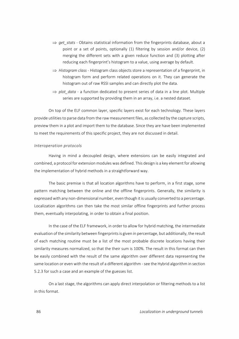
86 Localization in underground tunnels
get_stats - Obtains statistical information from the fingerprints database, about a
point or a set of points, optionally (1) filtering by session and/or device, (2)
merging the different sets with a given reduce function and (3) plotting after
reducing each fingerprint’s histogram to a value, using average by default.
Histogram class - Histogram class objects store a representation of a fingerprint, in
histogram form and perform related operations on it. They can generate the
histogram out of raw RSSI samples and can directly plot the data.
plot_data - a function dedicated to present series of data in a line plot. Multiple
series are supported by providing them in an array, i.e. a nested dataset.
On top of the ELF common layer, specific layers exist for each technology. These layers
provide utilities to parse data from the raw measurement files, as collected by the capture scripts,
preview them in a plot and import them to the database. Since they are have been implemented
to meet the requirements of this specific project, they are not discussed in detail.
Interoperation protocols
Having in mind a decoupled design, where extensions can be easily integrated and
combined, a protocol for extension modules was defined. This design is a key element for allowing
the implementation of hybrid methods in a straightforward way.
The basic premise is that all location algorithms have to perform, in a first stage, some
pattern matching between the online and the offline fingerprints. Generally, the similarity is
expressed with any non-dimensional number, even though it is usually converted to a percentage.
Localization algorithms can then take the most similar offline fingerprints and further process
them, eventually interpolating, in order to obtain a final position.
In the case of the ELF framework, in order to allow for hybrid matching, the intermediate
evaluation of the similarity between fingerprints is given in percentage, but additionally, the result
of each matching routine must be a list of the most probable discrete locations having their
similarity measures normalized, so that the their sum is 100%. The result in this format can then
be easily combined with the result of the same algorithm over different data representing the
same location or even with the result of a different algorithm - see the Hybrid algorithm in section
5.2.3 for such a case and an example of the guesses list.
On a last stage, the algorithms can apply direct interpolation or filtering methods to a list
in this format.
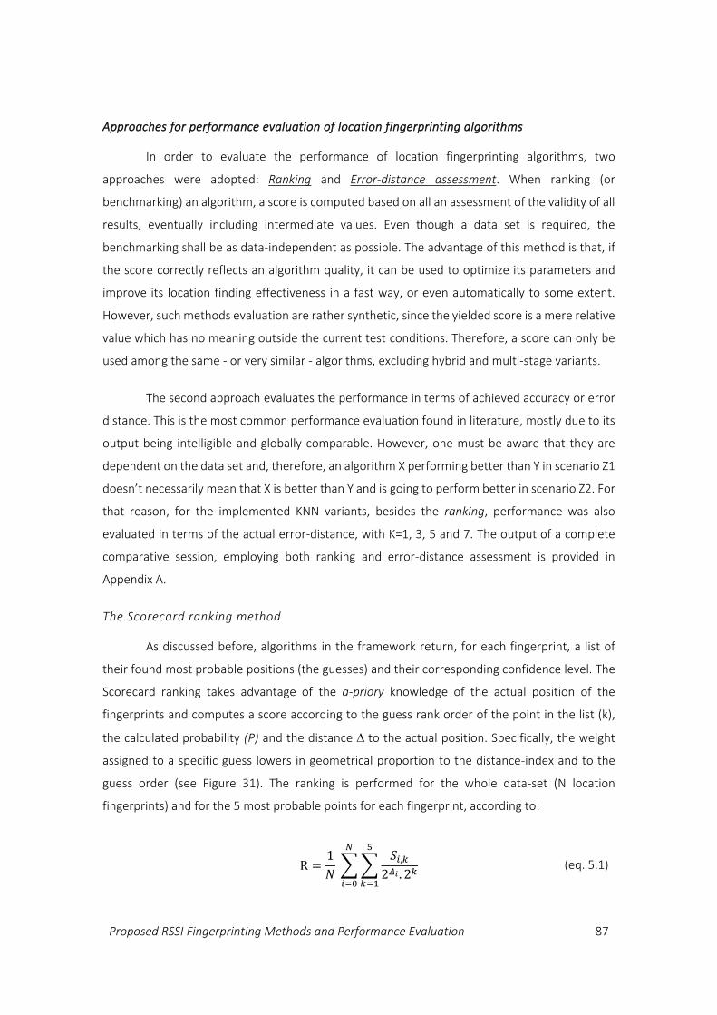
Proposed RSSI Fingerprinting Methods and Performance Evaluation 87
Approaches for performance evaluation of location fingerprinting algorithms
In order to evaluate the performance of location fingerprinting algorithms, two
approaches were adopted: Ranking and Error-distance assessment. When ranking (or
benchmarking) an algorithm, a score is computed based on all an assessment of the validity of all
results, eventually including intermediate values. Even though a data set is required, the
benchmarking shall be as data-independent as possible. The advantage of this method is that, if
the score correctly reflects an algorithm quality, it can be used to optimize its parameters and
improve its location finding effectiveness in a fast way, or even automatically to some extent.
However, such methods evaluation are rather synthetic, since the yielded score is a mere relative
value which has no meaning outside the current test conditions. Therefore, a score can only be
used among the same - or very similar - algorithms, excluding hybrid and multi-stage variants.
The second approach evaluates the performance in terms of achieved accuracy or error
distance. This is the most common performance evaluation found in literature, mostly due to its
output being intelligible and globally comparable. However, one must be aware that they are
dependent on the data set and, therefore, an algorithm X performing better than Y in scenario Z1
doesn’t necessarily mean that X is better than Y and is going to perform better in scenario Z2. For
that reason, for the implemented KNN variants, besides the ranking, performance was also
evaluated in terms of the actual error-distance, with K=1, 3, 5 and 7. The output of a complete
comparative session, employing both ranking and error-distance assessment is provided in
Appendix A.
The Scorecard ranking method
As discussed before, algorithms in the framework return, for each fingerprint, a list of
their found most probable positions (the guesses) and their corresponding confidence level. The
Scorecard ranking takes advantage of the a-priory knowledge of the actual position of the
fingerprints and computes a score according to the guess rank order of the point in the list (k),
the calculated probability (P) and the distance to the actual position. Specifically, the weight
assigned to a specific guess lowers in geometrical proportion to the distance-index and to the
guess order (see Figure 31). The ranking is performed for the whole data-set (N location
fingerprints) and for the 5 most probable points for each fingerprint, according to:
R =1
𝑁 ∑∑
𝑆𝑖,𝑘2𝛥𝑖 . 2𝑘
5
𝑘=1
𝑁
𝑖=0
(eq. 5.1)
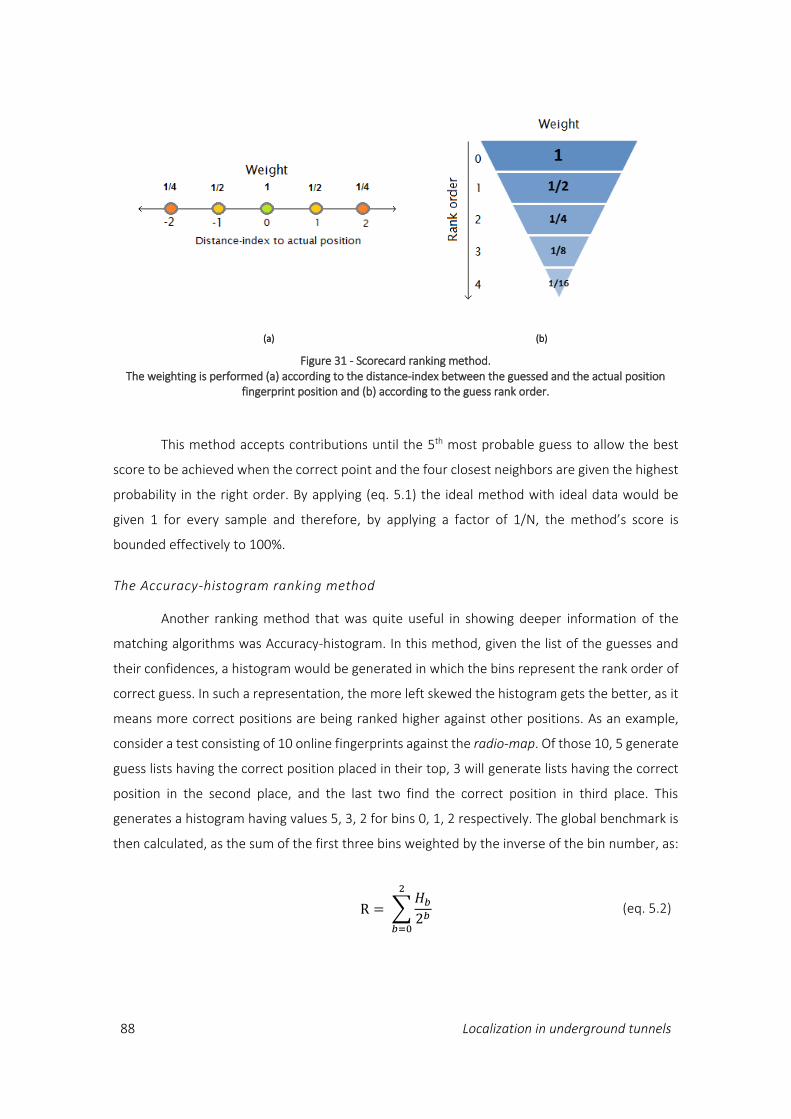
88 Localization in underground tunnels
This method accepts contributions until the 5th most probable guess to allow the best
score to be achieved when the correct point and the four closest neighbors are given the highest
probability in the right order. By applying (eq. 5.1) the ideal method with ideal data would be
given 1 for every sample and therefore, by applying a factor of 1/N, the method’s score is
bounded effectively to 100%.
The Accuracy-histogram ranking method
Another ranking method that was quite useful in showing deeper information of the
matching algorithms was Accuracy-histogram. In this method, given the list of the guesses and
their confidences, a histogram would be generated in which the bins represent the rank order of
correct guess. In such a representation, the more left skewed the histogram gets the better, as it
means more correct positions are being ranked higher against other positions. As an example,
consider a test consisting of 10 online fingerprints against the radio-map. Of those 10, 5 generate
guess lists having the correct position placed in their top, 3 will generate lists having the correct
position in the second place, and the last two find the correct position in third place. This
generates a histogram having values 5, 3, 2 for bins 0, 1, 2 respectively. The global benchmark is
then calculated, as the sum of the first three bins weighted by the inverse of the bin number, as:
R = ∑𝐻𝑏2𝑏
2
𝑏=0
(eq. 5.2)
(a) (b)
Figure 31 - Scorecard ranking method. The weighting is performed (a) according to the distance-index between the guessed and the actual position
fingerprint position and (b) according to the guess rank order.

Proposed RSSI Fingerprinting Methods and Performance Evaluation 89
5.2 PROPOSED LOCALIZATION ALGORITHMS
Among the location fingerprinting algorithms, those based on the k-Nearest-Neighbor
are particularly interesting due to their relative simplicity to implement, flexibility to incorporate
new pattern matching methods and the fact that they generally perform very well even when
compared to other - usually more complex - algorithms. Their performance was found to be
alongside with other deterministic and probabilistic approaches (Honkavirta, et al., 2009), or even
superior, when compared for instance to Artificial Neural Networks (Lin & Lin, 2005).
The developed location fingerprinting algorithms are therefore based in KNN, having
their pattern matching routines and parameters customized to meet the characteristics of the
experiment.
5.2.1 MODIFIED GENERAL-PURPOSE WEIGHTED KNN
In weighted-KNN approaches, additional information is taken into account when
evaluating the matching of an online and an offline fingerprint. These additional factors are
translated into weights, which are applied to the distance between the points (eq. 2.20).
A new weighting method accounting for fingerprint measurement conditions
In the scenario of the LHC tunnel, as observed in the previous part, the measurements
can be quite stable as long as they were collected in optimal conditions (Figure 23). When the
conditions start to be less ideal, the fingerprints distributions’ get larger and their means and
medians are less reliable.
To introduce that factor in the computation of the fingerprints distance a new weighting
method was investigated. This method builds on the following premises:
The narrower the fingerprint distribution the better it represents the RSSI and the more
reliable it is.
A wider distribution means there is more uncertainty, as opposed to dissimilarity, and
therefore a good fingerprint agreement shall not directly be negatively weighted.
Considering fingerprints whose mean values are “N” dB apart, there’s better agreement
if both present large distributions which partially overlap, than narrow distributions
which completely separate.

90 Localization in underground tunnels
These premises lead to the implementation of a weighting method which considers the
overlapping between the online and offline fingerprint distributions. The method calculates the
weight, per bin, as the probability density sitting outside the bin normalized distance - see Figure
32.
Implementation
As an initial step, a generic KNN fingerprinting algorithm was implemented which could
be highly parametrized. This flexibility allowed the test and optimization of the several
parameters with the existing radio-map.
Equations (eq. 2.16) and (eq. 2.20) are the foundation for a generic KNN algorithm. From
their analysis one can see that can be implemented in software in a simple way while leaving the
parameters openly configurable. Furthermore, if one keeps the separation of the roles, as
suggested by the two separate equations, one can formulate a localization algorithm as having in
its base a fingerprinting matching method (e.g. a distance-norm measurement as in (eq. 2.16)),
followed by a location estimation phase, like KNN as in (eq. 2.20). The first approach was
nevertheless to implement KNN as a direct translation of these equations, as shown in the
following two code blocks, respectively.
Figure 32 - Weighting according to the CDF approximate
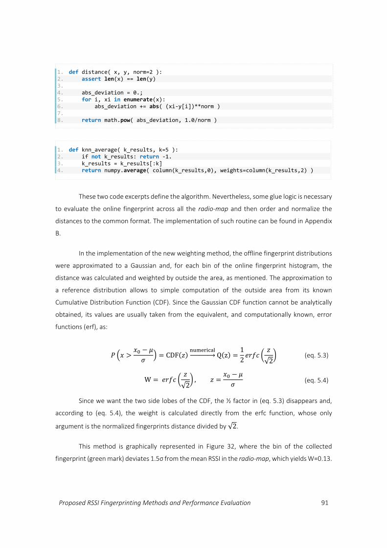
Proposed RSSI Fingerprinting Methods and Performance Evaluation 91
These two code excerpts define the algorithm. Nevertheless, some glue logic is necessary
to evaluate the online fingerprint across all the radio-map and then order and normalize the
distances to the common format. The implementation of such routine can be found in Appendix
B.
In the implementation of the new weighting method, the offline fingerprint distributions
were approximated to a Gaussian and, for each bin of the online fingerprint histogram, the
distance was calculated and weighted by outside the area, as mentioned. The approximation to
a reference distribution allows to simple computation of the outside area from its known
Cumulative Distribution Function (CDF). Since the Gaussian CDF function cannot be analytically
obtained, its values are usually taken from the equivalent, and computationally known, error
functions (erf), as:
𝑃 (𝑥 >𝑥0 − 𝜇
𝜎) = CDF(𝑧)
numerical→ Q(z) =
1
2𝑒𝑟𝑓𝑐 (
𝑧
√2) (eq. 5.3)
W = 𝑒𝑟𝑓𝑐 (𝑧
√2) , 𝑧 =
𝑥0 − 𝜇
𝜎 (eq. 5.4)
Since we want the two side lobes of the CDF, the ½ factor in (eq. 5.3) disappears and,
according to (eq. 5.4), the weight is calculated directly from the erfc function, whose only
argument is the normalized fingerprints distance divided by √2.
This method is graphically represented in Figure 32, where the bin of the collected
fingerprint (green mark) deviates 1.5σ from the mean RSSI in the radio-map, which yields W=0.13.
1. def distance( x, y, norm=2 ): 2. assert len(x) == len(y) 3. 4. abs_deviation = 0.; 5. for i, xi in enumerate(x): 6. abs_deviation += abs( (xi-y[i])**norm ) 7. 8. return math.pow( abs_deviation, 1.0/norm )
1. def knn_average( k_results, k=5 ): 2. if not k_results: return -1. 3. k_results = k_results[:k] 4. return numpy.average( column(k_results,0), weights=column(k_results,2) )
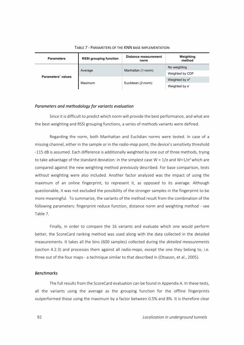
92 Localization in underground tunnels
Parameters and methodology for variants evaluation
Since it is difficult to predict which norm will provide the best performance, and what are
the best weighting and RSSI grouping functions, a series of methods variants were defined.
Regarding the norm, both Manhattan and Euclidian norms were tested. In case of a
missing channel, either in the sample or in the radio-map point, the device’s sensitivity threshold
-115 dB is assumed. Each difference is additionally weighted by one out of three methods, trying
to take advantage of the standard deviation: in the simplest case W = 1/σ and W=1/σ2 which are
compared against the new weighting method previously described. For base comparison, tests
without weighting were also included. Another factor analyzed was the impact of using the
maximum of an online fingerprint, to represent it, as opposed to its average. Although
questionable, it was not excluded the possibility of the stronger samples in the fingerprint to be
more meaningful. To summarize, the variants of the method result from the combination of the
following parameters: fingerprint reduce function, distance norm and weighting method - see
Table 7.
Finally, in order to compare the 16 variants and evaluate which one would perform
better, the ScoreCard ranking method was used along with the data collected in the detailed
measurements. It takes all the bins (600 samples) collected during the detailed measurements
(section 4.2.3) and processes them against all radio-maps, except the one they belong to, i.e.
three out of the four maps - a technique similar to that described in (Otsason, et al., 2005).
Benchmarks
The full results from the ScoreCard evaluation can be found in Appendix A. In these tests,
all the variants using the average as the grouping function for the offline fingerprints
outperformed those using the maximum by a factor between 0.5% and 8%. It is therefore clear
TABLE 7 - PARAMETERS OF THE KNN BASE IMPLEMENTATION
Parameters RSSI grouping function Distance measurement
norm Weighting
method
Parameters’ values
Average Manhattan (1-norm) No weighting
Weighted by CDF
Maximum Euclidean (2-norm) Weighted by σ2
Weighted by σ
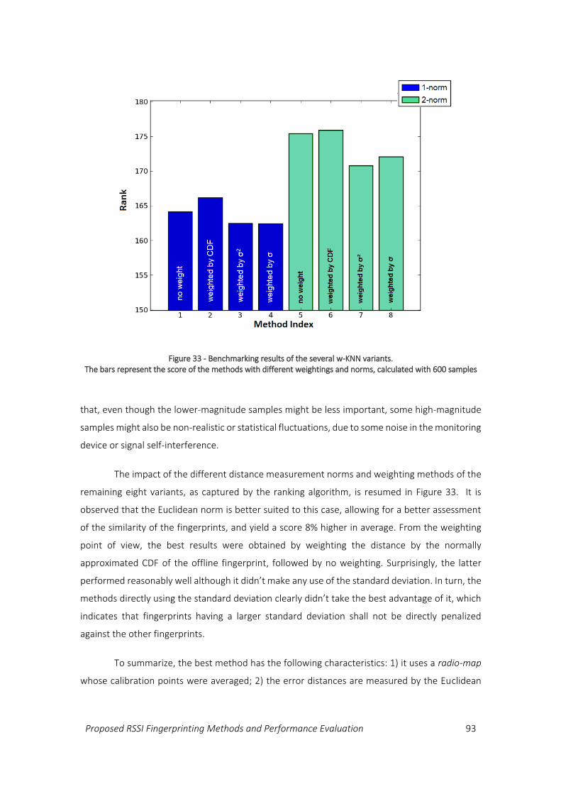
Proposed RSSI Fingerprinting Methods and Performance Evaluation 93
that, even though the lower-magnitude samples might be less important, some high-magnitude
samples might also be non-realistic or statistical fluctuations, due to some noise in the monitoring
device or signal self-interference.
The impact of the different distance measurement norms and weighting methods of the
remaining eight variants, as captured by the ranking algorithm, is resumed in Figure 33. It is
observed that the Euclidean norm is better suited to this case, allowing for a better assessment
of the similarity of the fingerprints, and yield a score 8% higher in average. From the weighting
point of view, the best results were obtained by weighting the distance by the normally
approximated CDF of the offline fingerprint, followed by no weighting. Surprisingly, the latter
performed reasonably well although it didn’t make any use of the standard deviation. In turn, the
methods directly using the standard deviation clearly didn’t take the best advantage of it, which
indicates that fingerprints having a larger standard deviation shall not be directly penalized
against the other fingerprints.
To summarize, the best method has the following characteristics: 1) it uses a radio-map
whose calibration points were averaged; 2) the error distances are measured by the Euclidean
Figure 33 - Benchmarking results of the several w-KNN variants. The bars represent the score of the methods with different weightings and norms, calculated with 600 samples
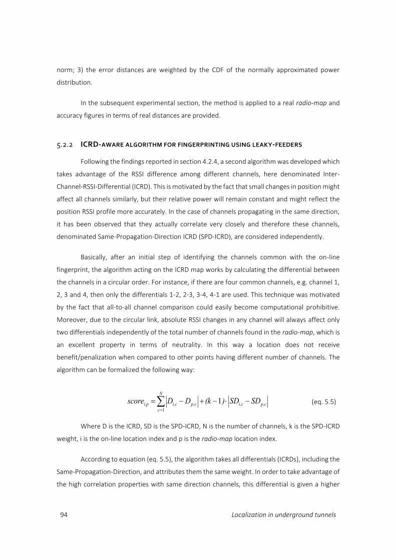
94 Localization in underground tunnels
norm; 3) the error distances are weighted by the CDF of the normally approximated power
distribution.
In the subsequent experimental section, the method is applied to a real radio-map and
accuracy figures in terms of real distances are provided.
5.2.2 ICRD-AWARE ALGORITHM FOR FINGERPRINTING USING LEAKY-FEEDERS
Following the findings reported in section 4.2.4, a second algorithm was developed which
takes advantage of the RSSI difference among different channels, here denominated Inter-
Channel-RSSI-Differential (ICRD). This is motivated by the fact that small changes in position might
affect all channels similarly, but their relative power will remain constant and might reflect the
position RSSI profile more accurately. In the case of channels propagating in the same direction,
it has been observed that they actually correlate very closely and therefore these channels,
denominated Same-Propagation-Direction ICRD (SPD-ICRD), are considered independently.
Basically, after an initial step of identifying the channels common with the on-line
fingerprint, the algorithm acting on the ICRD map works by calculating the differential between
the channels in a circular order. For instance, if there are four common channels, e.g. channel 1,
2, 3 and 4, then only the differentials 1-2, 2-3, 3-4, 4-1 are used. This technique was motivated
by the fact that all-to-all channel comparison could easily become computational prohibitive.
Moreover, due to the circular link, absolute RSSI changes in any channel will always affect only
two differentials independently of the total number of channels found in the radio-map, which is
an excellent property in terms of neutrality. In this way a location does not receive
benefit/penalization when compared to other points having different number of channels. The
algorithm can be formalized the following way:
p,ci,c
N
c
p,ci,ci,p SDSD)(kDDscore 1
1
(eq. 5.5)
Where D is the ICRD, SD is the SPD-ICRD, N is the number of channels, k is the SPD-ICRD
weight, i is the on-line location index and p is the radio-map location index.
According to equation (eq. 5.5), the algorithm takes all differentials (ICRDs), including the
Same-Propagation-Direction, and attributes them the same weight. In order to take advantage of
the high correlation properties with same direction channels, this differential is given a higher

Proposed RSSI Fingerprinting Methods and Performance Evaluation 95
weight (k), but since it had been considered once in the summation part of the equation, the
weight becomes (k-1).
Implementation
In order to implement the presented method as part of the Location framework, the
previous expression was translated to software functions. In fact the algorithm was initially
implemented in a direct way, following the conceptually required two steps: first, the calculation
of the ICRDs; second, the comparison of the ICRDs between the radio-map and the fingerprint.
Such implementation is very simple and can be represented by the following pseudo-code:
Nevertheless, such implementation lacks the flexibility required to cope with eventual
incomplete or incompatible delta sets, e.g. when a fingerprint didn’t capture all (sometime any
of) the channels present in the radio-map, a very common situation even for samples taken in
the same point. Therefore the equations were transformed to simplify the process and relax the
requirement of having completely matching ICRD sets.
The transformation is based on the aggregation of terms from the same channel, as
shown in (eq. 5.6).
1. def point_calc_difs( channels_rssi ): 2. # This is the implementation of the direct method 3. """We expect a list in the format [[channel, val],...] """ 4. 5. dif_channels = [] 6. dif_values = [] 7. 8. for i,[ch1, val1] in enumerate(channels_rssi[:-1]): 9. #Forward difs 10. [ch2, val2] = channels_rssi[i+1] #Next 11. dif_channels.append( [ch1, ch2] ) 12. dif_values.append( val1 - val2 ) 13. 14. #Dif between first and last 15. ch1, val1 = channels_rssi[0] 16. ch2, val2 = channels_rssi[-1] 17. dif_channels.append( [ch1, ch2] ) 18. dif_values.append( val1 - val2 ) 19. 20. return dif_channels, dif_values
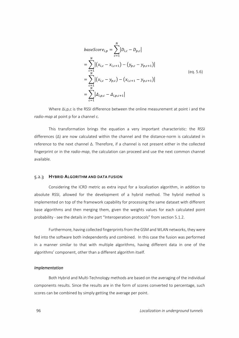
96 Localization in underground tunnels
𝑏𝑎𝑠𝑒𝑆𝑐𝑜𝑟𝑒𝑖,𝑝 =∑|𝐷𝑖,𝑐 − 𝐷𝑝,𝑐|
𝑁
𝑐=1
=∑|(𝑥𝑖,𝑐 − 𝑥𝑖,𝑐+1) − (𝑦𝑝,𝑐 − 𝑦𝑝,𝑐+1)|
𝑁
𝑐=1
=∑|(𝑥𝑖,𝑐 − 𝑦𝑝,𝑐) − (𝑥𝑖,𝑐+1 − 𝑦𝑝,𝑐+1)|
𝑁
𝑐=1
=∑|𝛥𝑖,𝑝,𝑐 − 𝛥𝑖,𝑝,𝑐+1|
𝑁
𝑐=1
(eq. 5.6)
Where Δi,p,c is the RSSI difference between the online measurement at point i and the
radio-map at point p for a channel c.
This transformation brings the equation a very important characteristic: the RSSI
differences (Δ) are now calculated within the channel and the distance-norm is calculated in
reference to the next channel Δ. Therefore, if a channel is not present either in the collected
fingerprint or in the radio-map, the calculation can proceed and use the next common channel
available.
5.2.3 HYBRID ALGORITHM AND DATA FUSION
Considering the ICRD metric as extra input for a localization algorithm, in addition to
absolute RSSI, allowed for the development of a hybrid method. The hybrid method is
implemented on top of the framework capability for processing the same dataset with different
base algorithms and then merging them, given the weights values for each calculated point
probability - see the details in the part “Interoperation protocols” from section 5.1.2.
Furthermore, having collected fingerprints from the GSM and WLAN networks, they were
fed into the software both independently and combined. In this case the fusion was performed
in a manner similar to that with multiple algorithms, having different data in one of the
algorithms’ component, other than a different algorithm itself.
Implementation
Both Hybrid and Multi-Technology methods are based on the averaging of the individual
components results. Since the results are in the form of scores converted to percentage, such
scores can be combined by simply getting the average per point.
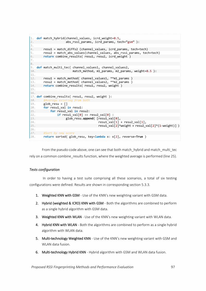
Proposed RSSI Fingerprinting Methods and Performance Evaluation 97
From the pseudo-code above, one can see that both match_hybrid and match_multi_tec
rely on a common combine_results function, where the weighted average is performed (line 25).
Tests configuration
In order to having a test suite comprising all these scenarios, a total of six testing
configurations were defined. Results are shown in corresponding section 5.3.3.
1. Weighted KNN with GSM - Use of the KNN’s new weighting variant with GSM data.
2. Hybrid (weighted & ICRD) KNN with GSM - Both the algorithms are combined to perform
as a single hybrid algorithm with GSM data.
3. Weighted KNN with WLAN - Use of the KNN’s new weighting variant with WLAN data.
4. Hybrid KNN with WLAN - Both the algorithms are combined to perform as a single hybrid
algorithm with WLAN data.
5. Multi-technology Weighted KNN - Use of the KNN’s new weighting variant with GSM and
WLAN data fusion.
6. Multi-technology Hybrid KNN - Hybrid algorithm with GSM and WLAN data fusion.
1. def match_hybrid(channel_values, icrd_weight=0.5, 2. abs_rssi_params, icrd_params, tech=”gsm” ): 3. 4. resu1 = match_diffs2 (channel_values, icrd_params, tech=tech) 5. resu2 = match_abs_values(channel_values, abs_rssi_params, tech=tech) 6. return combine_results( resu1, resu2, icrd_weight ) 7. 8. 9. def match_multi_tec( channel_values1, channel_values2, 10. match_method, m1_params, m2_params, weight=0.5 ): 11. 12. resu1 = match_method( channel_values1, **m1_params ) 13. resu2 = match_method( channel_values2, **m2_params ) 14. return combine_results( resu1, resu2, weight ) 15. 16. 17. def combine_results( resu1, resu2, weight ): 18. #Average existing from both 19. glob_resu = [] 20. for resu1_val in resu1: 21. for resu2_val in resu2: 22. if resu1_val[0] == resu2_val[0] : 23. glob_resu.append( [resu1_val[0], 24. resu1_val[1] + resu2_val[1], 25. resu1_val[2]*weight + resu2_val[2]*(1-weight)] ) 26. 27. #Sort by new score 28. return sorted( glob_resu, key=lambda x: x[2], reverse=True )
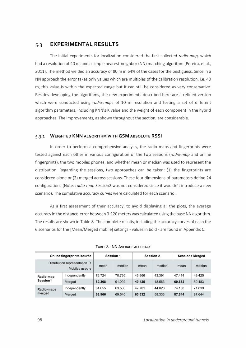
98 Localization in underground tunnels
5.3 EXPERIMENTAL RESULTS
The initial experiments for localization considered the first collected radio-map, which
had a resolution of 40 m, and a simple nearest-neighbor (NN) matching algorithm (Pereira, et al.,
2011). The method yielded an accuracy of 80 m in 64% of the cases for the best guess. Since in a
NN approach the error takes only values which are multiples of the calibration resolution, i.e. 40
m, this value is within the expected range but it can still be considered as very conservative.
Besides developing the algorithms, the new experiments described here are a refined version
which were conducted using radio-maps of 10 m resolution and testing a set of different
algorithm parameters, including KNN’s K value and the weight of each component in the hybrid
approaches. The improvements, as shown throughout the section, are considerable.
5.3.1 WEIGHTED KNN ALGORITHM WITH GSM ABSOLUTE RSSI
In order to perform a comprehensive analysis, the radio maps and fingerprints were
tested against each other in various configuration of the two sessions (radio-map and online
fingerprints), the two mobiles phones, and whether mean or median was used to represent the
distribution. Regarding the sessions, two approaches can be taken: (1) the fingerprints are
considered alone or (2) merged across sessions. These four dimensions of parameters define 24
configurations (Note: radio-map Session2 was not considered since it wouldn’t introduce a new
scenario). The cumulative accuracy curves were calculated for each scenario.
As a first assessment of their accuracy, to avoid displaying all the plots, the average
accuracy in the distance-error between 0-120 meters was calculated using the base NN algorithm.
The results are shown in Table 8. The complete results, including the accuracy curves of each the
6 scenarios for the [Mean/Merged mobile] settings - values in bold - are found in Appendix C.
TABLE 8 - NN AVERAGE ACCURACY
Online fingerprints source Session 1 Session 2 Sessions Merged
Distribution representation
Mobiles used ↴ mean median mean median mean median
Radio-map Session1
Independently 76.724 78.736 43.966 43.391 47.414 49.425
Merged 89.368 91.092 49.425 48.563 60.632 59.483
Radio-maps merged
Independently 64.655 63.506 47.701 44.828 74.138 71.839
Merged 68.966 69.540 60.632 58.333 87.644 87.644
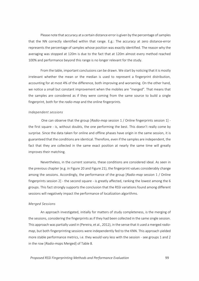
Proposed RSSI Fingerprinting Methods and Performance Evaluation 99
Please note that accuracy at a certain distance error is given by the percentage of samples
that the NN correctly identified within that range. E.g.: The accuracy at zero distance-error
represents the percentage of samples whose position was exactly identified. The reason why the
averaging was stopped at 120m is due to the fact that at 120m almost every method reached
100% and performance beyond this range is no longer relevant for the study.
From the table, important conclusions can be drawn. We start by noticing that it is mostly
irrelevant whether the mean or the median is used to represent a fingerprint distribution,
accounting for at most 4% of the difference, both improving and worsening. On the other hand,
we notice a small but constant improvement when the mobiles are “merged”. That means that
the samples are considered as if they were coming from the same source to build a single
fingerprint, both for the radio-map and the online fingerprints.
Independent sessions
One can observe that the group [Radio-map session 1 / Online fingerprints session 1] -
the first square - is, without doubts, the one performing the best. This doesn’t really come by
surprise. Since the data taken for online and offline phases have origin in the same session, it is
guaranteed that the conditions are identical. Therefore, even if the samples are independent, the
fact that they are collected in the same exact position at nearly the same time will greatly
improves their matching.
Nevertheless, in the current scenario, these conditions are considered ideal. As seen in
the previous chapter (e.g. in Figure 20 and Figure 21), the fingerprint values considerably change
among the sessions. Accordingly, the performance of the group [Radio-map session 1 / Online
fingerprints session 2] - the second square - is greatly affected, ranking the lowest among the 6
groups. This fact strongly supports the conclusion that the RSSI variations found among different
sessions will negatively impact the performance of localization algorithms.
Merged Sessions
An approach investigated, initially for matters of study completeness, is the merging of
the sessions, considering the fingerprints as if they had been collected in the same single session.
This approach was partially used in (Pereira, et al., 2012), in the sense that it used a merged radio-
map, but both fingerprinting sessions were independently fed to the KNN. This approach yielded
more stable performance metrics, i.e. they would vary less with the session - see groups 1 and 2
in the row [Radio-maps Merged] of Table 8.
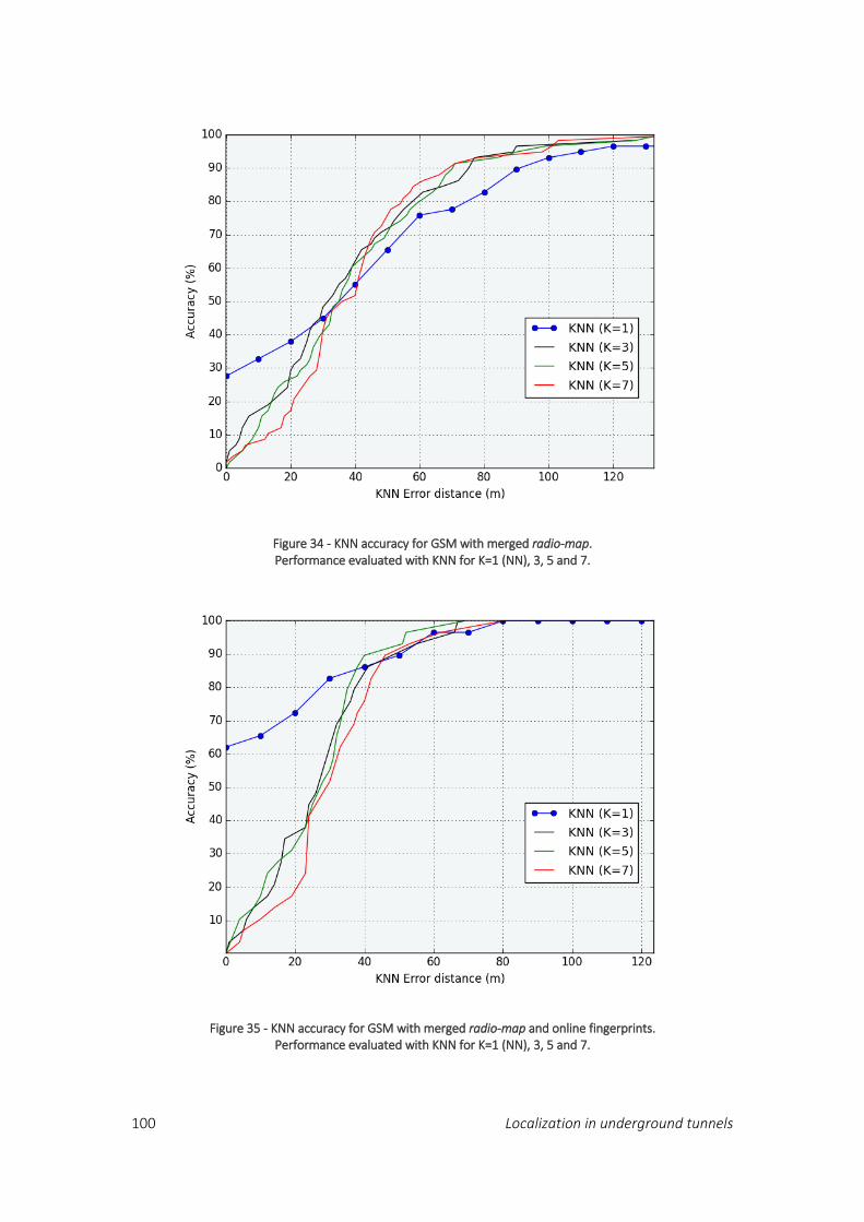
100 Localization in underground tunnels
Figure 34 - KNN accuracy for GSM with merged radio-map. Performance evaluated with KNN for K=1 (NN), 3, 5 and 7.
Figure 35 - KNN accuracy for GSM with merged radio-map and online fingerprints. Performance evaluated with KNN for K=1 (NN), 3, 5 and 7.
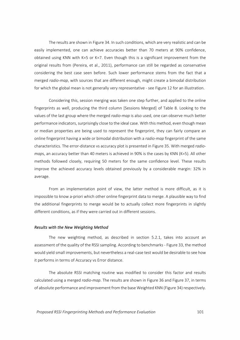
Proposed RSSI Fingerprinting Methods and Performance Evaluation 101
The results are shown in Figure 34. In such conditions, which are very realistic and can be
easily implemented, one can achieve accuracies better than 70 meters at 90% confidence,
obtained using KNN with K=5 or K=7. Even though this is a significant improvement from the
original results from (Pereira, et al., 2011), performance can still be regarded as conservative
considering the best case seen before. Such lower performance stems from the fact that a
merged radio-map, with sources that are different enough, might create a bimodal distribution
for which the global mean is not generally very representative - see Figure 12 for an illustration.
Considering this, session merging was taken one step further, and applied to the online
fingerprints as well, producing the third column [Sessions Merged] of Table 8. Looking to the
values of the last group where the merged radio-map is also used, one can observe much better
performance indicators, surprisingly close to the ideal case. With this method, even though mean
or median properties are being used to represent the fingerprint, they can fairly compare an
online fingerprint having a wide or bimodal distribution with a radio-map fingerprint of the same
characteristics. The error-distance vs accuracy plot is presented in Figure 35. With merged radio-
maps, an accuracy better than 40 meters is achieved in 90% is the cases by KNN (K=5). All other
methods followed closely, requiring 50 meters for the same confidence level. These results
improve the achieved accuracy levels obtained previously by a considerable margin: 32% in
average.
From an implementation point of view, the latter method is more difficult, as it is
impossible to know a-priori which other online fingerprint data to merge. A plausible way to find
the additional fingerprints to merge would be to actually collect more fingerprints in slightly
different conditions, as if they were carried out in different sessions.
Results with the New Weighting Method
The new weighting method, as described in section 5.2.1, takes into account an
assessment of the quality of the RSSI sampling. According to benchmarks - Figure 33, the method
would yield small improvements, but nevertheless a real-case test would be desirable to see how
it performs in terms of Accuracy vs Error distance.
The absolute RSSI matching routine was modified to consider this factor and results
calculated using a merged radio-map. The results are shown in Figure 36 and Figure 37, in terms
of absolute performance and improvement from the base Weighted KNN (Figure 34) respectively.
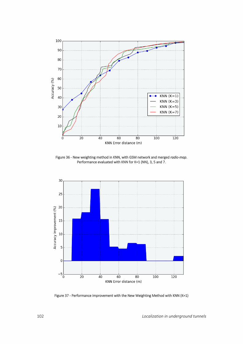
102 Localization in underground tunnels
Figure 36 - New weighting method in KNN, with GSM network and merged radio-map. Performance evaluated with KNN for K=1 (NN), 3, 5 and 7.
Figure 37 - Performance improvement with the New Weighting Method with KNN (K=1)
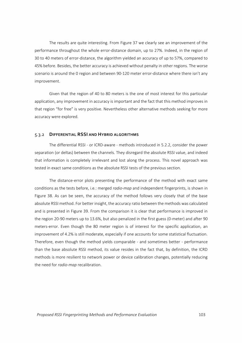
Proposed RSSI Fingerprinting Methods and Performance Evaluation 103
The results are quite interesting. From Figure 37 we clearly see an improvement of the
performance throughout the whole error-distance domain, up to 27%. Indeed, in the region of
30 to 40 meters of error-distance, the algorithm yielded an accuracy of up to 57%, compared to
45% before. Besides, the better accuracy is achieved without penalty in other regions. The worse
scenario is around the 0 region and between 90-120 meter error-distance where there isn’t any
improvement.
Given that the region of 40 to 80 meters is the one of most interest for this particular
application, any improvement in accuracy is important and the fact that this method improves in
that region “for free” is very positive. Nevertheless other alternative methods seeking for more
accuracy were explored.
5.3.2 DIFFERENTIAL RSSI AND HYBRID ALGORITHMS
The differential RSSI - or ICRD-aware - methods introduced in 5.2.2, consider the power
separation (or deltas) between the channels. They disregard the absolute RSSI value, and indeed
that information is completely irrelevant and lost along the process. This novel approach was
tested in exact same conditions as the absolute RSSI tests of the previous section.
The distance-error plots presenting the performance of the method with exact same
conditions as the tests before, i.e.: merged radio-map and independent fingerprints, is shown in
Figure 38. As can be seen, the accuracy of the method follows very closely that of the base
absolute RSSI method. For better insight, the accuracy ratio between the methods was calculated
and is presented in Figure 39. From the comparison it is clear that performance is improved in
the region 20-90 meters up to 13.6%, but also penalized in the first guess (0-meter) and after 90
meters-error. Even though the 80 meter region is of interest for the specific application, an
improvement of 4.2% is still moderate, especially if one accounts for some statistical fluctuation.
Therefore, even though the method yields comparable - and sometimes better - performance
than the base absolute RSSI method, its value resides in the fact that, by definition, the ICRD
methods is more resilient to network power or device calibration changes, potentially reducing
the need for radio-map recalibration.
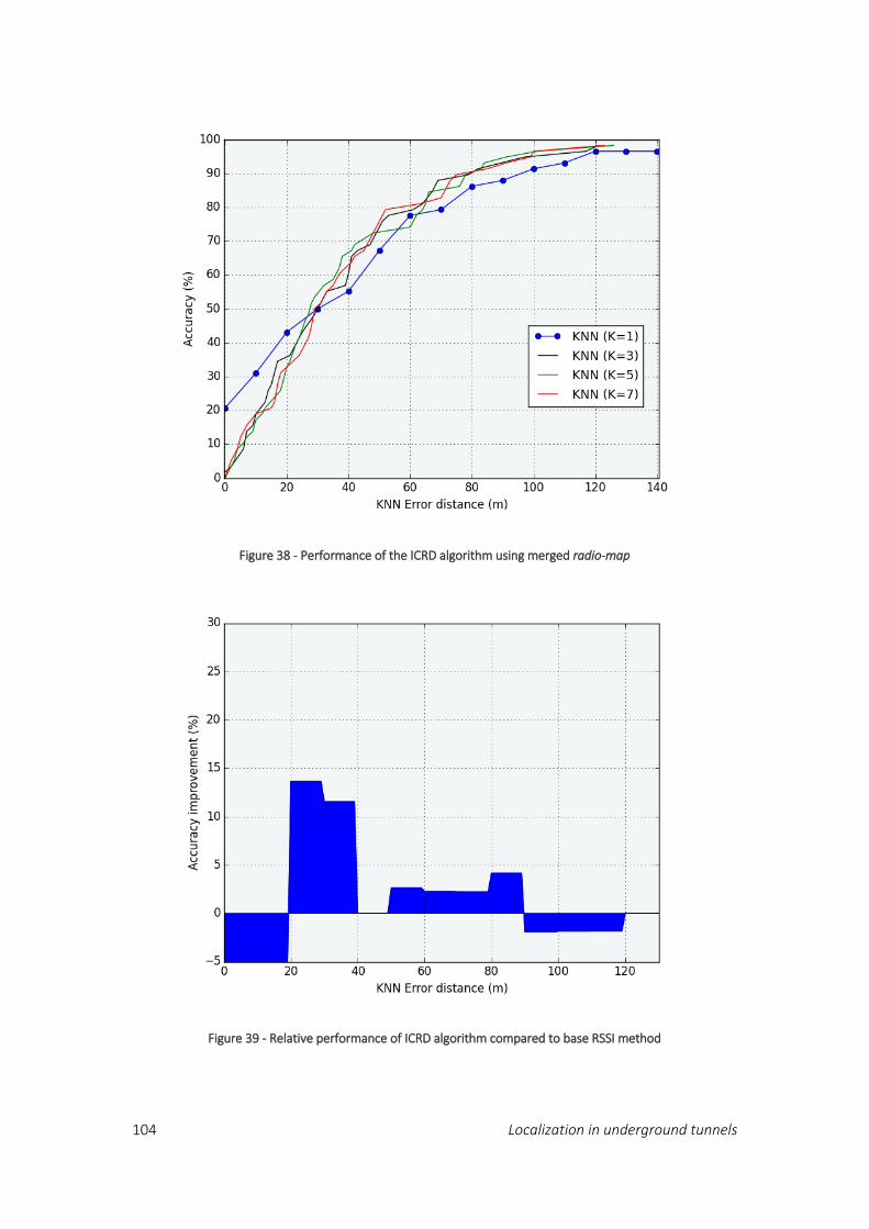
104 Localization in underground tunnels
Figure 38 - Performance of the ICRD algorithm using merged radio-map
Figure 39 - Relative performance of ICRD algorithm compared to base RSSI method
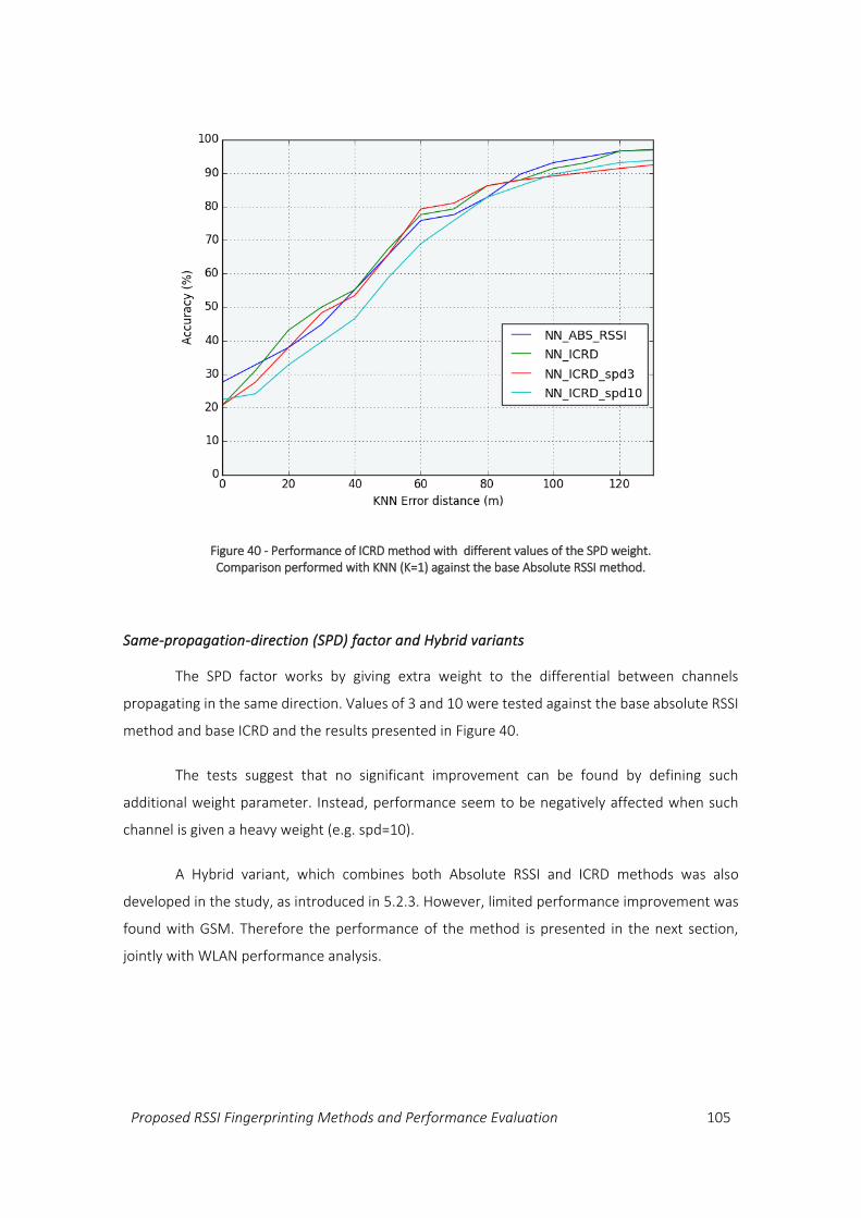
Proposed RSSI Fingerprinting Methods and Performance Evaluation 105
Same-propagation-direction (SPD) factor and Hybrid variants
The SPD factor works by giving extra weight to the differential between channels
propagating in the same direction. Values of 3 and 10 were tested against the base absolute RSSI
method and base ICRD and the results presented in Figure 40.
The tests suggest that no significant improvement can be found by defining such
additional weight parameter. Instead, performance seem to be negatively affected when such
channel is given a heavy weight (e.g. spd=10).
A Hybrid variant, which combines both Absolute RSSI and ICRD methods was also
developed in the study, as introduced in 5.2.3. However, limited performance improvement was
found with GSM. Therefore the performance of the method is presented in the next section,
jointly with WLAN performance analysis.
Figure 40 - Performance of ICRD method with different values of the SPD weight. Comparison performed with KNN (K=1) against the base Absolute RSSI method.

106 Localization in underground tunnels
5.3.3 PERFORMANCE WITH WLAN AND IMPACT OF DATA FUSION
WLAN experiments are relevant to the current study for two main reasons. First it
provides an insight on the performance in case such technology becomes permanently adopted
in tunnels used at CERN. Second, it allows us to understand whether the relatively moderate
performance levels achieved with GSM are also due to the technical properties of the network,
especially that RSSI are generally low and little changing due to the leaky feeder. The data
collection setup is the same as presented in Section 4.3, featuring the two Access Points and
shield foils.
As a first localization test (Pereira, et al., 2012), the average error of all the online
fingerprints was calculated for all ABS_RSSI, ICRD and HYBRID algorithms with KNN K values of 1,
3, 5 and 7. The test was applied to both GSM and WLAN networks and accuracy results as plotted
as a function of KNN values - see Figure 41. Second, the typical accuracy vs Error-distance plot is
computed with the exact same parameters as for GSM, i.e.: merged radio-map, independent
fingerprints - see Figure 42.
In Figure 41(a) it is noticeable that, with GSM, the performance of all methods gets better
as more locations (K) are considered by KNN. This might be due to the fact that, with such little
differences in absolute value, finding the exact match of a location is very difficult and averaging
the best guesses weighted by their degree of confidence indeed becomes a favorable option.
With WLAN - Figure 41(b) and Figure 42 - one can clearly observe a significantly better
overall performance. In particular the Absolute RSSI matching method performs better than the
(a) (b)
Figure 41 - Performance of the various KNN algorithms evaluated with GSM and WLAN
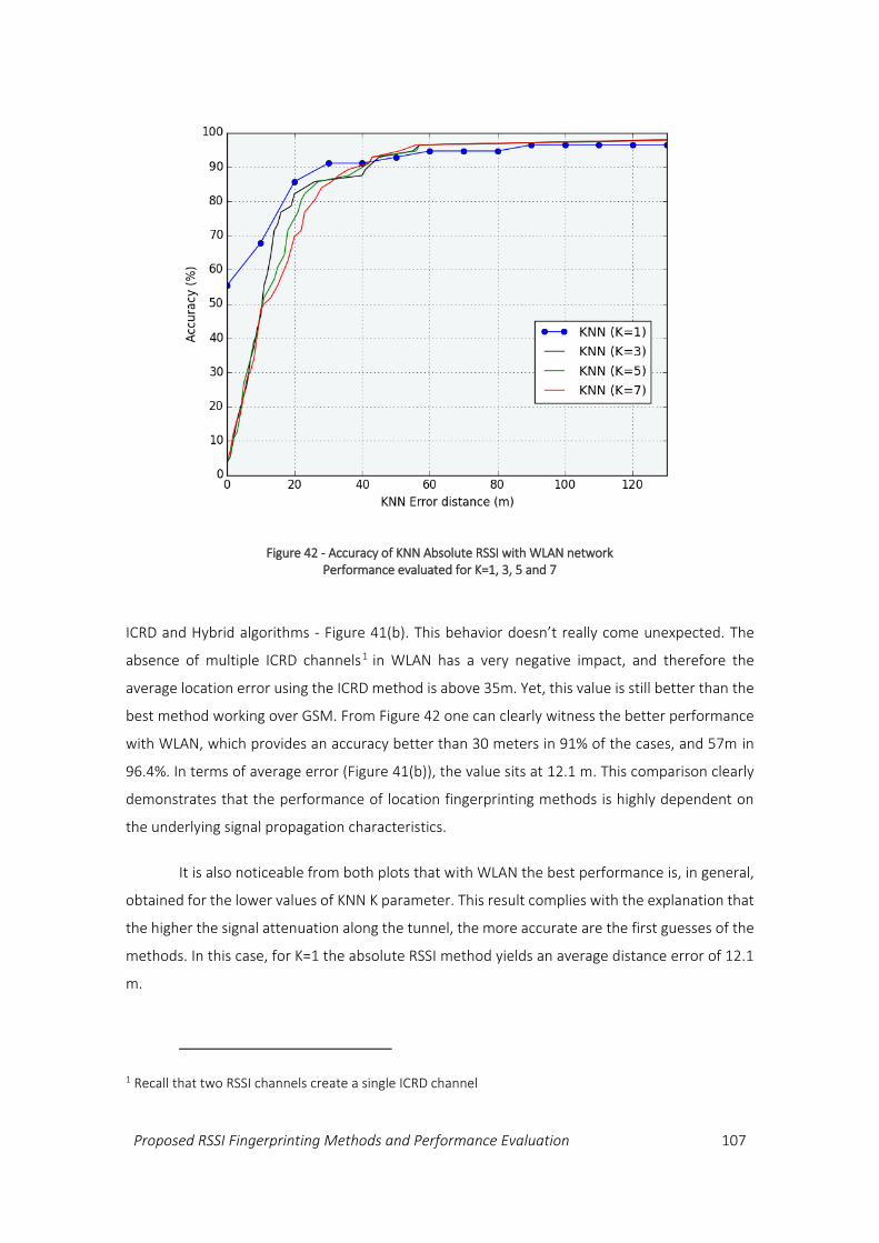
Proposed RSSI Fingerprinting Methods and Performance Evaluation 107
ICRD and Hybrid algorithms - Figure 41(b). This behavior doesn’t really come unexpected. The
absence of multiple ICRD channels1 in WLAN has a very negative impact, and therefore the
average location error using the ICRD method is above 35m. Yet, this value is still better than the
best method working over GSM. From Figure 42 one can clearly witness the better performance
with WLAN, which provides an accuracy better than 30 meters in 91% of the cases, and 57m in
96.4%. In terms of average error (Figure 41(b)), the value sits at 12.1 m. This comparison clearly
demonstrates that the performance of location fingerprinting methods is highly dependent on
the underlying signal propagation characteristics.
It is also noticeable from both plots that with WLAN the best performance is, in general,
obtained for the lower values of KNN K parameter. This result complies with the explanation that
the higher the signal attenuation along the tunnel, the more accurate are the first guesses of the
methods. In this case, for K=1 the absolute RSSI method yields an average distance error of 12.1
m.
1 Recall that two RSSI channels create a single ICRD channel
Figure 42 - Accuracy of KNN Absolute RSSI with WLAN network Performance evaluated for K=1, 3, 5 and 7
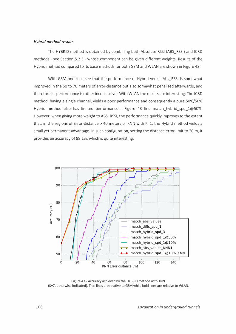
108 Localization in underground tunnels
Hybrid method results
The HYBRID method is obtained by combining both Absolute RSSI (ABS_RSSI) and ICRD
methods - see Section 5.2.3 - whose component can be given different weights. Results of the
Hybrid method compared to its base methods for both GSM and WLAN are shown in Figure 43.
With GSM one case see that the performance of Hybrid versus Abs_RSSI is somewhat
improved in the 50 to 70 meters of error-distance but also somewhat penalized afterwards, and
therefore its performance is rather inconclusive. With WLAN the results are interesting. The ICRD
method, having a single channel, yields a poor performance and consequently a pure 50%/50%
Hybrid method also has limited performance - Figure 43 line match_hybrid_spd_1@50%.
However, when giving more weight to ABS_RSSI, the performance quickly improves to the extent
that, in the regions of Error-distance > 40 meters or KNN with K=1, the Hybrid method yields a
small yet permanent advantage. In such configuration, setting the distance error limit to 20 m, it
provides an accuracy of 88.1%, which is quite interesting.
Figure 43 - Accuracy achieved by the HYBRID method with KNN (K=7, otherwise indicated). Thin lines are relative to GSM while bold lines are relative to WLAN.
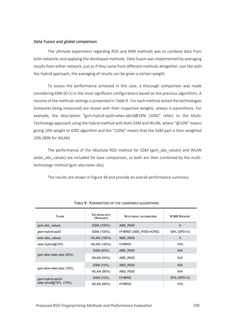
Proposed RSSI Fingerprinting Methods and Performance Evaluation 109
Data Fusion and global comparison
The ultimate experiment regarding RSSI and KNN methods was to combine data from
both networks and applying the developed methods. Data fusion was implemented by averaging
results from either network, just as if they came from different methods altogether. Just like with
the Hybrid approach, the averaging of results can be given a certain weight.
To assess the performance achieved in this case, a thorough comparison was made
considering KNN (K=1) in the most significant configurations based on the previous algorithms. A
resume of the methods settings is presented in Table 9 . For each method tested the technologies
(networks being measured) are shown with their respective weights, always in parenthesis. For
example, the description “gsm-hybrid-spd3+wlan-ybrid@10% (10%)” refers to the Multi-
Technology approach using the hybrid method with both GSM and WLAN, where “@10%” means
giving 10% weight to ICRD algorithm and the “(10%)” means that the GSM part is then weighted
10% (90% for WLAN)
The performance of the Absolute RSSI method for GSM (gsm_abs_values) and WLAN
(wlan_abs_values) are included for base comparison, as both are then combined by the multi-
technology method (gsm-abs+wlan-abs).
The results are shown in Figure 44 and provide an overall performance summary.
TABLE 9 - PARAMETERS OF THE COMPARED ALGORITHMS
NAME TECHNOLOGY
(WEIGHT) MATCHING ALGORITHM ICRD WEIGHT
gsm-abs_values GSM (100%) ABS_RSSI 0
gsm-hybrid-spd3 GSM (100%) HYBRID (ABS_RSSI+ICRD) 50% (SPD=3)
wlan-abs_values WLAN (100%) ABS_RSSI 0
wlan-hybrid@10% WLAN (100%) HYBRID 10%
gsm-abs+wlan-abs (50%)
GSM (50%) ABS_RSSI N/A
WLAN (50%) ABS_RSSI N/A
gsm-abs+wlan-abs (10%) GSM (10%) ABS_RSSI N/A
WLAN (90%) ABS_RSSI N/A
gsm-hybrid-spd3+ wlan-ybrid@10% (10%)
GSM (10%) HYBRID 50% (SPD=3)
WLAN (90%) HYBRID 10%

110 Localization in underground tunnels
The results show again, now with KNN, K=1 in all cases, the significant performance
improvement obtained when the algorithms work over WLAN. Even when combining both
technologies giving 50%/50% weights, the performance of this multi-technology method largely
exceeds that from GSM alone, and approaches the one from WLAN. However, only when giving
10% weight to GSM – method gsm-abs+wlan-abs(10%) – the global performance improves and
achieves the same level as WLAN itself.
When combining hybrid methods from the different technologies (gsm-hybrid-
spd3+wlan-hybrid@10%), a similar behavior is observed. The algorithm yields an accuracy level
identical to that achieved by the best underlying algorithm – wlan-hybrid@10% in this case. The
fact that the multi-technology method doesn’t improve on that result might be due to the highly
uneven levels of accuracy achieved by the underlying technologies. Furthermore, in order to
improve the already rather accurate guess with WLAN, one would need quite high confidence
levels in the GSM matching (uncommon in the current data set) and eventually a location
algorithm, other than KNN, that could take better advantage of the combined result set.
Figure 44 - Accuracy comparison among the various methods Absolute RSSI, Hybrid and Multi-Technology evaluated with KNN (K=1).
Please note that red and yellow lines are totally coincident, while green and purple lines also coincide except for one point.
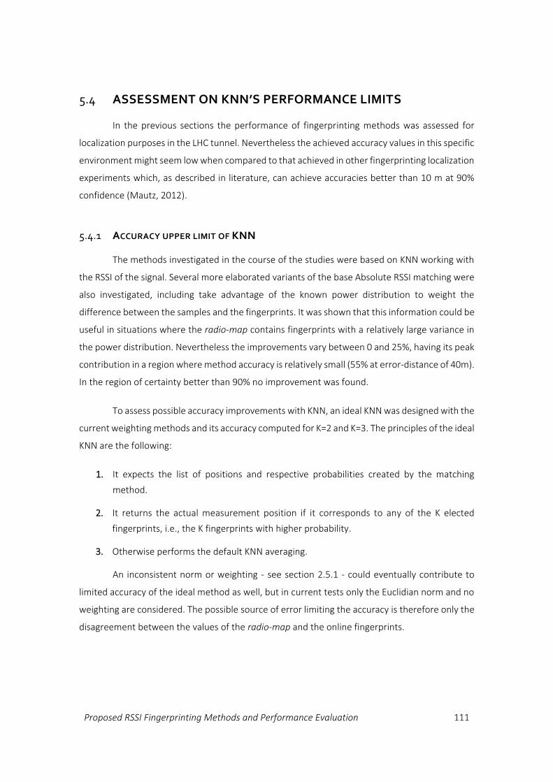
Proposed RSSI Fingerprinting Methods and Performance Evaluation 111
5.4 ASSESSMENT ON KNN’S PERFORMANCE LIMITS
In the previous sections the performance of fingerprinting methods was assessed for
localization purposes in the LHC tunnel. Nevertheless the achieved accuracy values in this specific
environment might seem low when compared to that achieved in other fingerprinting localization
experiments which, as described in literature, can achieve accuracies better than 10 m at 90%
confidence (Mautz, 2012).
5.4.1 ACCURACY UPPER LIMIT OF KNN
The methods investigated in the course of the studies were based on KNN working with
the RSSI of the signal. Several more elaborated variants of the base Absolute RSSI matching were
also investigated, including take advantage of the known power distribution to weight the
difference between the samples and the fingerprints. It was shown that this information could be
useful in situations where the radio-map contains fingerprints with a relatively large variance in
the power distribution. Nevertheless the improvements vary between 0 and 25%, having its peak
contribution in a region where method accuracy is relatively small (55% at error-distance of 40m).
In the region of certainty better than 90% no improvement was found.
To assess possible accuracy improvements with KNN, an ideal KNN was designed with the
current weighting methods and its accuracy computed for K=2 and K=3. The principles of the ideal
KNN are the following:
1. It expects the list of positions and respective probabilities created by the matching
method.
2. It returns the actual measurement position if it corresponds to any of the K elected
fingerprints, i.e., the K fingerprints with higher probability.
3. Otherwise performs the default KNN averaging.
An inconsistent norm or weighting - see section 2.5.1 - could eventually contribute to
limited accuracy of the ideal method as well, but in current tests only the Euclidian norm and no
weighting are considered. The possible source of error limiting the accuracy is therefore only the
disagreement between the values of the radio-map and the online fingerprints.

112 Localization in underground tunnels
The ideal KNN was initially tested with the first network data collection (Pereira, et al.,
2011), where the calibration was performed every 40 meters. The results are shown in Figure 45,
and express a considerable improvement of the accuracy. It was found that the ideal KNN taking
advantage of the three best-matched fingerprints (3-NN) could increase the accuracy by 27% in
the best case. It should also be noted that the advantage of the 3-NN over the 2-NN approach is
at best about 10%.
Although the results with the ideal KNN method are very interesting, they looked poor in
the global scene, as to achieve an accuracy of 80% the error distance is up to 80m. Nevertheless,
we must take into consideration the conditions in which the tests and more specifically, the
calibration were performed. In fact, given that the resolution of the current radio map is 40 m,
80 m correspond to the distance between three subsequent calibration points. If hypothetically
our environment could offer the same signal characteristics for a radio-map taken with a
resolution of 1 m, the achieved accuracy would then be in the order of 2 m for this ideal method
and 3 m for our method, for a confidence of 80%.
Such rationale was one argument towards the higher resolution calibration phase - 10
meters - as presented throughout this thesis.
Figure 45 - Performance of the ideal KNN, for K=2 and K=3, compared to NN. Initial GSM studies with a 40 m resolution radio-map
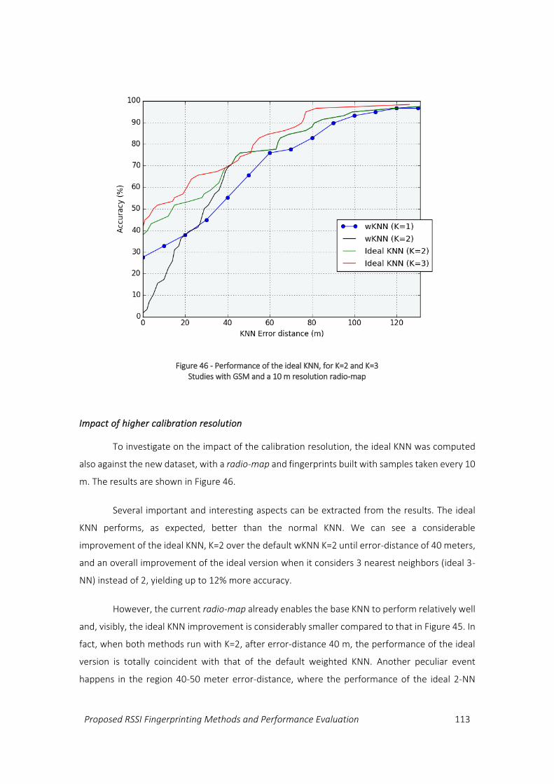
Proposed RSSI Fingerprinting Methods and Performance Evaluation 113
Impact of higher calibration resolution
To investigate on the impact of the calibration resolution, the ideal KNN was computed
also against the new dataset, with a radio-map and fingerprints built with samples taken every 10
m. The results are shown in Figure 46.
Several important and interesting aspects can be extracted from the results. The ideal
KNN performs, as expected, better than the normal KNN. We can see a considerable
improvement of the ideal KNN, K=2 over the default wKNN K=2 until error-distance of 40 meters,
and an overall improvement of the ideal version when it considers 3 nearest neighbors (ideal 3-
NN) instead of 2, yielding up to 12% more accuracy.
However, the current radio-map already enables the base KNN to perform relatively well
and, visibly, the ideal KNN improvement is considerably smaller compared to that in Figure 45. In
fact, when both methods run with K=2, after error-distance 40 m, the performance of the ideal
version is totally coincident with that of the default weighted KNN. Another peculiar event
happens in the region 40-50 meter error-distance, where the performance of the ideal 2-NN
Figure 46 - Performance of the ideal KNN, for K=2 and K=3 Studies with GSM and a 10 m resolution radio-map
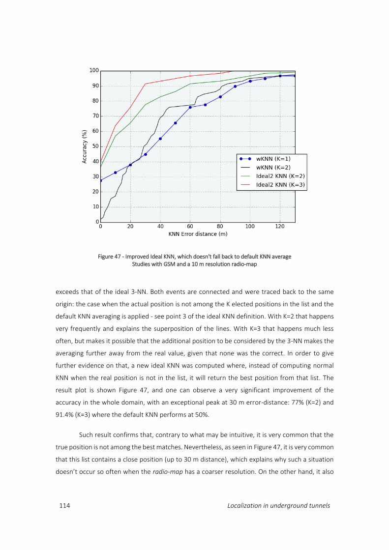
114 Localization in underground tunnels
exceeds that of the ideal 3-NN. Both events are connected and were traced back to the same
origin: the case when the actual position is not among the K elected positions in the list and the
default KNN averaging is applied - see point 3 of the ideal KNN definition. With K=2 that happens
very frequently and explains the superposition of the lines. With K=3 that happens much less
often, but makes it possible that the additional position to be considered by the 3-NN makes the
averaging further away from the real value, given that none was the correct. In order to give
further evidence on that, a new ideal KNN was computed where, instead of computing normal
KNN when the real position is not in the list, it will return the best position from that list. The
result plot is shown Figure 47, and one can observe a very significant improvement of the
accuracy in the whole domain, with an exceptional peak at 30 m error-distance: 77% (K=2) and
91.4% (K=3) where the default KNN performs at 50%.
Such result confirms that, contrary to what may be intuitive, it is very common that the
true position is not among the best matches. Nevertheless, as seen in Figure 47, it is very common
that this list contains a close position (up to 30 m distance), which explains why such a situation
doesn’t occur so often when the radio-map has a coarser resolution. On the other hand, it also
Figure 47 - Improved Ideal KNN, which doesn't fall back to default KNN average Studies with GSM and a 10 m resolution radio-map
Proposed RSSI Fingerprinting Methods and Performance Evaluation 115
happens frequently that the K-elected positions are relatively far from the real point, and
therefore the default KNN averaging is largely surpassed by a truly ideal situation that only the
closest point is selected and the others discarded.
5.4.2 OTHER FACTORS LIMITING ACCURACY
Even though conditions for reliable signal stability can certainly be found in many static
environments, the tests carried out in the underground suggest that under normal working
conditions in an underground tunnel, where other pieces of bulky and massive equipment and
personnel are present, such conditions are hardly possible to achieve. That implies that the
differences between measurement sessions are significant and therefore that the matching
algorithms often don’t correctly find the nearest position, or include positions which are relatively
far away.
It should also be noted that in addition to the specific and unique nature of the
accelerator equipment in the tunnel also their operation conditions might change at times, like
the power conditions of magnets. Even though no specific studies on the influence of these
parameters have been done yet, it cannot be fully excluded that there might be an impact.
Regarding the radio-map resolution, there was a notable improvement from 40 m to 10
m calibration distance. Further tests have been performed to assess the performance for a
calibration with a resolution in the order of 1 meter. It was found that the spatial and in-time
fluctuations of the network electromagnetic fields overwhelms the signal small attenuation
caused by propagation along a leaky feeder. Eventually other networks, where the RSSI is
expected to vary in a shorter scale, might benefit from such high-resolution radio-maps.
116 Localization in underground tunnels
5.5 CONCLUSIONS
This chapter presented the experiments regarding localization performed using GSM and
WLAN signals in the LHC tunnel. It presents several KNN variants which, working over real RSSI
fingerprints, computed positions and their accuracy was evaluated in terms of error-distance and
accuracy percentage (or confidence).
The base-comparison method is a direct implementation of the weighted KNN, amply
mentioned in related literature. Given that two data sessions are available, several approaches of
data merging are studied. The approach in which merging happens in both the radio-map and the
fingerprints are highly effective, reaching with GSM accuracies better than 50 m in 90% of the
cases. Nevertheless, given the difficult practicality of the approach, the base approach selected
for the next experiments is that of the merged radio-map only. With the plain weighted KNN
method it yields accuracies limited to 70 m error in 90% of the cases.
Among the new explored approaches are a KNN method with a new weighting factor,
which takes into account the fingerprints distribution, the ICRD method, which takes advantage
of the channels RSSI differential, and a hybrid approach. When considering GSM, the first
approach shows to improve accuracy in the region up to 90 m error by a factor of up to 27%
higher, without harming accuracy in any accuracy zone. The ICRD method showed a performance
compatible with that of the base method, but its strength relies on the potential reduction of the
need for recalibration. The Hybrid approach was found to achieve as well comparable results as
the base method.
Tests with WLAN were performed in similar conditions and allow for much better
accuracies. One can reach 30 m of maximum distance-error in 91 % of the cases with base
weighted KNN, and a small improvement (1 to 2% more) when using the hybrid method. A Multi-
Technology approach was tested as well, where computations from both networks were taken
into account. Nevertheless the GSM contribution could not help the Hybrid method to improve
the interesting accuracy levels obtained by WLAN itself, achieving only coincident performance.
As last, an ideal KNN was modeled to provide a better understanding on the accuracy
upper limits of RSSI fingerprinting approaches with KNN applied to the current data. It was found
that with a 40 m resolution GSM radio-map the improvement is reasonably constant along all the
error-distance domain, increasing the accuracy by up to 27% more, while in 10 m resolution radio-
map the possible improvement is moderate. This is due to the higher probability of the K-best
Proposed RSSI Fingerprinting Methods and Performance Evaluation 117
matches to not include the correct position of the measurement. In those cases, if instead of
defaulting to the KNN averaging one selects the closest location, accuracy is considerably
increased again, up to 30m error-distance at 91% confidence.
Such test provides a good hint that the underlying matching methods are actually quite
effective in selecting good matches. However, it is virtually impossible to achieve a KNN
implementations reaching those performance limits, since the information required to select the
best locations doesn’t exist in a real situation, and in the ideal case they were artificially fed into
the calculation. Unless other measured information, other than the RSSI, are fed to the KNN or
time-evolution techniques (e.g. filters) are applied, to better rank the possible positions, the
performance with KNN seems quite limited to those accuracy figures achieved before, in the
same range found with the weighted KNN approaches.

118 Localization in underground tunnels
Enhancing Localization Accuracy with Narrowband Techniques 119
Chapter 6
ENHANCING LOCALIZATION ACCURACY
WITH NARROWBAND TECHNIQUES
This chapter presents the design of a complementary localization system capable of
achieving higher accuracy levels, and its validation via a prototype implemented using SDR, in
contrast to dedicated hardware. The following sections introduce the principles behind phase-
delay positioning and SDRs, the conducted experiments, the developed methods, their
implementation and, finally, their performance. In the end an overview of a joint localization
system using both RSSI fingerprinting and phase-delay is presented.
6.1 INTRODUCTION
For the purpose of localization in the CERN accelerator tunnels, techniques based on RSSI
fingerprinting have been previously explored, which took advantage of the dense network
coverage available via a set of leaky-feeder cables. Even though RSSI-based methods have shown
to be effective in estimating the location their best accuracy was achieved with WLAN and was
limited to 20m at a confidence level of 88%. With GSM the accuracy was limited to 70m at 90%
confidence in realistic conditions, which is not sufficient for providing an accurate position tag for
some applications.
6.1.1 MOTIVATION AND OBJECTIVES
Besides the benefit with respect to increased personal safety, a good level of accuracy,
in the order of one to two meters, would enable for much faster processes carried out by various
technical departments at CERN, including radiation surveys with automatic position tagging. In
order to increase the accuracy up to the envisaged levels, techniques based on Time-of-Flight (RF
wave propagation delay), that could meet the tunnels restrictions and specificities, have been
120 Localization in underground tunnels
investigated. By measuring the carrier phase-delay in the VHF band (2m wavelength), the
technology aims at achieving 1 meter-level accuracy and, by propagating the signal over the leaky-
feeder cable, full tunnel coverage is expected to be achieved with a small number of units. With
the purpose of validating the approach and, at the same time, prove that alternatives to the
traditional integrated-circuit approach exist, the algorithms were prototyped using
programmable Software Defined Radio (SDR) devices.
6.1.2 OPPORTUNITY FOR TOF USING PHASE-DELAY
Technologies based in Time-of-Flight - see section 2.3.1 - are arguably those enabling for
the highest accuracy levels, typically reaching resolutions better than 30 cm in a 3D coordinate
system. Nevertheless, due to the very high propagation speed and multi-path effects, these
techniques generally require synchronization between the elements - e.g. GPS - or to send very
short pulses whose delay is measured. The latter technique is known as ultra-wideband (UWB)
due to its large spectrum consumption. In both cases the implementation is quite naturally done
in hardware due to the strict requirements in terms of signal processing. Due to the several
reasons presented before, including the impossibility of developing and installing hardware in the
tunnel, such approach is not viable to the current project.
The only option available is therefore to work in narrowband. If one considers delay
measurement of the signal itself, without messages or pulses, it is actually conceivable obtaining
a time-delay from the measurement of the phase of a carrier signal, which would theoretically
not occupy any spectrum. Tests with audible frequencies were explored in (Viegas, 2005). Due to
that, the processing requirements of the devices are much less strict and open the possibility of
implementing them in software, tuned to the current scenario. On the other hand, having a signal
that virtually doesn’t occupy any band greatly reduces the risk of interference with existing
hardware installed in the tunnel. Such property enabled the studies to comply with the hard
restrictions imposed by the tunnel policies in-place, and therefore to proceed and being tested.
At the same time of the development of the current PhD work, a network being
previously used for safety purposes entered its decommissioning phase. This network used
frequencies in the VHF band and was, along with GSM, transmitted throughout the tunnel via the
leaky-feeder cable system. Given that frequencies in the VHF band seem to be in the same range
as those required for the localization signal, the decommissioning of the previous network seems
Enhancing Localization Accuracy with Narrowband Techniques 121
an excellent opportunity to the current work, which can benefit from existing VHF infrastructure
and the guarantee that there’s no interference in that spectrum region.
6.1.3 ADVANTAGES OF SDR
The SDR approach stands as a very interesting approach mostly due to its prototype
friendly characteristics:
1. Fast development: The development time might get greatly reduced due to the
availability of signal processing software libraries.
2. Fast development-to-test iterations: With SDR, there is no need of reprogramming or
sending the device to be assembled. The SDR platform runs the code directly.
3. Relatively low development costs: For the same reasons as (2), costs are only associated
with SDR devices, and will not increase with the number of development iterations.
Given that phase-delay techniques require little band and relatively little computation,
SDR seems an excellent approach as long as the devices are capable of sampling rates obeying
Nyquist criteria for the designed signal.
6.2 PHASE-DELAY POSITIONING AND SDR
Phase-delay methods are an alternative to UWB positioning and the techniques for
obtaining the measure are quite different. UWB frequently employs pseudo-random noise (PRN)
codes so that auto-correlation techniques can be applied at the receiver. Among the best known
cases is GPS C/A (GPS.gov, 2014; Ávila Rodríguez, 2011) which employs Gold Codes of 1023 chips
at 1 Mchip/s whose receivers are currently able to detect shifts in the order of 1% of chip time.
That is 1% x 1 µs = 10 ns which, at the speed of light, represents a spatial accuracy of around 3 m.
6.2.1 PHASE-DELAY TECHNIQUES
In systems using narrower frequency bands, even though multiple propagation paths can
be more difficult to distinguish, the carrier phase can be recovered at the receiver. In these cases
the accuracy is proportional to the wavelength, typically up to 1%, and therefore cm-level
accuracy can be reached as well.
122 Localization in underground tunnels
Phase delay techniques work fundamentally with pure sinusoidal waves from which the
phase is to be recovered. Nevertheless, some bandwidth is normally required. Firstly for target
disambiguation (or identification) in case the location is computed by a central unit. Secondly,
and depending on the design, some elements of the system may have to be synchronized,
typically between the sender and the receiver or among several emitters. This requirement
introduces an additional need for transmitting either synchronization messages or several
reference sinusoidal waves, which in both cases can be considered as band. Besides identification
and synchronization, a third aspect is often desirable: extended range. Considering 5% accuracy
in phase detection, 10 cm of spatial accuracy requires 2 m wavelength signals. Without
disambiguation, two meters would therefore be the localization range, which might be too short
for many applications. These aspects are briefly introduced and define the foundations of the
developed technique.
Phase detection and drift correction
In perfect conditions, the phase can be directly detected by very simple circuits which are
indeed called phase detectors or phase comparators. They are an essential element of Phase-
locked-Loops (PLLs), widely used to generate waves themselves. PLLs are simple and nowadays
implemented as highly integrated circuits, and so became an economical mass-production
answer to the electronics industry needs, notably supporting the wireless revolution (Barrett,
1999). Despite impressive evolution over the years, PLLs are not ideal and their quality can be
assessed, among other, by their frequency accuracy and jitter (phase noise). Such limitation is
associated with the crystal oscillator used which, for commodity Temperature Compensated
Crystal Oscillators (TCXOs), is commonly found to be around +/-2.5 ppm over -30ºC to +75ºC.
(Cerda, 2005). Even though 2.5 ppm might sound extraordinary, it translates to a frequency shift
of up to 100 Hz on a 25 MHz wave, which is enormous for phase sensitive applications.
To compensate for the mentioned limitations, two alternatives exist: employing a drift
correction signal or using the same clock (and device) for both wave generation and phase
detection which implies a round-trip architecture. Both methods were explored in this thesis.
Round-trip methods are conceptually simpler, but are nevertheless technically challenging due to
requirement of no phase distortion along the path even though different frequencies must be
used for each direction. The implementation details or the latter are given in section 6.4.2.
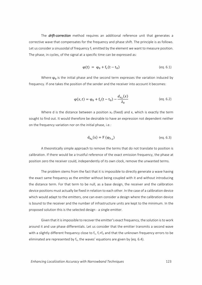
Enhancing Localization Accuracy with Narrowband Techniques 123
The drift-correction method requires an additional reference unit that generates a
corrective wave that compensates for the frequency and phase shift. The principle is as follows.
Let us consider a sinusoidal of frequency fc emitted by the element we want to measure position.
The phase, in cycles, of the signal at a specific time can be expressed as:
φ(t) = φ0 + f𝑐(t − t0) (eq. 6.1)
Where φ0 is the initial phase and the second term expresses the variation induced by
frequency. If one takes the position of the sender and the receiver into account it becomes:
φ(𝑥, 𝑡) = φ0 + fc(t − t0) −𝑑𝑥0(𝑥)
𝜆0 (eq. 6.2)
Where d is the distance between a position x0 (fixed) and x, which is exactly the term
sought to find out. It would therefore be desirable to have an expression not dependent neither
on the frequency variation nor on the initial phase, i.e.:
dx0(x) = F (φλ 0) (eq. 6.3)
A theoretically simple approach to remove the terms that do not translate to position is
calibration. If there would be a trustful reference of the exact emission frequency, the phase at
position zero the receiver could, independently of its own clock, remove the unwanted terms.
The problem stems from the fact that it is impossible to directly generate a wave having
the exact same frequency as the emitter without being coupled with it and without introducing
the distance term. For that term to be null, as a base design, the receiver and the calibration
device positions must actually be fixed in relation to each other. In the case of a calibration device
which would adapt to the emitters, one can even consider a design where the calibration device
is bound to the receiver and the number of infrastructure units are kept to the minimum. In the
proposed solution this is the selected design - a single emitter.
Given that it is impossible to recover the emitter’s exact frequency, the solution is to work
around it and use phase differentials. Let us consider that the emitter transmits a second wave
with a slightly different frequency close to fc, fc+fΔ and that the unknown frequency errors to be
eliminated are represented by fe, the waves’ equations are given by (eq. 6.4).

124 Localization in underground tunnels
{
φ1(𝑡) = φ0 + [fc + fe](𝑡 − 𝑡0) −
𝑑𝑥0(𝑥)
𝜆0
φ2(𝑡) = φ′0 + [fc + fΔ + fe](𝑡 − 𝑡0) −𝑑𝑥0(𝑥)
𝜆0
(eq. 6.4)
Where fe, at the receiver side, is not only the frequency shift caused by the clock drift at
the emitter, but also due to the clock drift at the receiver itself.
Based on these two signals, the reference unit can now create a third one (φ3) whose
phase difference to φ2 is the same as between φ1 and φ2, i.e.:
φ3(𝑡) − φ2(𝑡) = φ2(𝑡) − 𝜑1(𝑡) (eq. 6.5)
From the receiver’s perspective, the waves are
{
φ1(𝑡) = φ0 + [fc + fe](𝑡 − 𝑡0) −
𝑑𝑥0(𝑥)
𝜆0
φ2(𝑡) = φ′0 + [fc + fΔ + fe](𝑡 − 𝑡0) −𝑑𝑥0(𝑥)
𝜆0
φ3(𝑡) = φ′′0+ [(fc + 2 fΔ) + fe](𝑡 − 𝑡0) + φK
(eq. 6.6)
The advantage with φ3 is that it no longer depends on the distance 𝑑𝑥0(𝑥), but rather
on a constant phase shift φK which depends only on the transmission delay between the
reference unit and the receiver.
Taking the phase difference at the receiver between waves 2 and 3, one ends up with:
Δφ = φ′′0+ fΔ(𝑡 − 𝑡0) + φK −
dx0(x)
λ0 (eq. 6.7)
Considering that φ′′0
and φK are constants that must calibrated at startup, the only
requirement is to remove the fΔ(𝑡 − 𝑡0) term. By carefully choosing fΔ to be small enough, the
clock offset of a demodulator signal having frequency fΔ becomes negligible and the phase
dependent on dx0(x) only can be recovered.

Enhancing Localization Accuracy with Narrowband Techniques 125
Cycle disambiguation for extended range
In phase-delay methods the localization range is the signal’s wavelength. In order to
overcome such limitation, disambiguation between the different cycles (or epochs) must be
performed. Such disambiguation can, conceivably, be performed as a second step of the exact
same technique proposed before but using a longer wavelength. Such wavelength should
therefore meet the following requirements:
Allow for localization resolutions better than the fine-localization epoch.
Be long enough to cover an interesting range. In the case of the LHC tunnel, it would be
of most interest to cover a length longer than the resolution of the GSM RSSI methods
seen before, i.e. > 100 m or < 2 MHz (propagation in copper).
However, the emission of a wave directly in that frequency poses several difficulties. In
the first place, since it is in a different frequency band, one doesn’t have the guarantee that it
won’t interfere with existing equipment and therefore might face authorization issues. Secondly,
in order to avoid parallel demodulation paths or separate circuits, which would be impractical
with SDR, it is of most interest to generate and process waves that are close together to allow
performing a single conversion step between baseband and carrier.
The solution to the aforementioned problem is therefore to transmit a pair of waves
whose frequencies, say f1 and f2, are close but separated by the intended resulting frequency. As
a result, by demodulating one wave with the other in the receiver one would obtain the expected
wave. Taking advantage of the fact that one wave is already transmitted for fine-grain accuracy,
only one additional wave must be transmitted for the coarse-grain localization to be possible.
Since the additional wave must also implement a phase correction method, a set of three
additional frequencies, separated by fΔ , are required. Therefore, by having both techniques
simultaneously, a total of six waves are required around a carrier, as exemplified by Figure 48.
For reference of the actual frequencies being used, refer to implementation section in 6.4.1.
Figure 48 - Frequency plan using phase reference and epoch disambiguation techniques

126 Localization in underground tunnels
6.2.2 SOFTWARE DEFINED RADIO PLATFORMS
Radio systems have traditionally consisted of transceiver chains with several stages,
where the signal is converted to an intermediate frequency, filtered, then converted down to
baseband and finally demodulated. With the advent of fast and inexpensive digital signal
processors (DSPs), radio systems can now employ digital transceivers composed of a radio Front-
End followed by an analogue to digital converter (ADC) and finally by a Back-End responsible for
the further signal processing, like filtering and demodulation (Isomäki & Avessta, 2004).
The need for fast-paced development and prototyping has motivated the research for
ways on how to change the behavior of some digital blocks with minimum time and cost, i.e. turn
them software programmable (Mitola, 1995; SDR Forum, 1999). This class of transceivers is
known as Software–Defined Radios and uses either Field-Programmable Gate Arrays (FPGA) or
even General Purpose Processors (GPP) to perform digital operations equivalent to a traditional
analogue transceiver (Isomäki & Avessta, 2004; Valerio, 2008).
Despite the increased degree of flexibility achieved in such configuration, FPGAs and
more critically GPPs are intrinsically slower than Application Specific Integrated Circuits (ASIC).
Therefore the computational requirements of the application must be carefully assessed to be
sure they can be implemented in SDR. In the case of using GPPs, an intermediate FPGA is
commonly used to perform the most demanding operations and down sample the signal to lower
rates before sending them to the GPP. This configuration is the one evaluated in the current
study.
SDR Architectures
The heterodyne receiver, as described in beginning of the current section, has been the
most common RF front-end architecture. However, as SDR pushes the “digital” closer to the
antenna, new architectures have been conceived towards minimal analog front-ends, notably the
Direct Conversion and the Tuned RF receivers (Isomäki & Avessta, 2004).
Direct Conversion Receiver
The Direct Conversion Receiver (DCR) requires much less components and, due to its
suitability for multiple standards, has attracted attention for SDR. In the DCR, the signal is directly
down converted to baseband, being then Low-pass filtered and sampled. Excluding signal
amplifiers, usually before and after down-conversion, the architecture is as depicted in Figure 49.

Enhancing Localization Accuracy with Narrowband Techniques 127
DCRs typically perform sampling in quadrature and therefore implement two chains with
Analog-Digital Converters (ADC’s). The desired signals can later be selected by software filters.
DCR’s are “tuned” to a certain frequency band of interest, which makes them flexible.
However, changing the frequency of the oscillator takes a small period of time, which might be
too long to cope with certain applications. Moreover, down-converting the signal directly to base-
band induces phase noise from the local oscillator into the signal band. Therefore a very precise
local oscillator, or later signal processing might be required to correctly recover the signal.
Tuned RF Receiver
The Tuned RF (TRF) receiver further simplifies the architecture by removing the analog
down-conversion step. It performs analog-digital conversion of signal right after having passed a
band selective filter (BPF) and therefore, disregarding amplifiers1, consists of only 2 logical blocks.
Such architecture eliminates some of the shortcomings from the previous architecture,
like the oscillator phase noise being coupled to the signal, but presents hard feasibility challenges.
The main difficulty in creating a practical TRF receiver is the limitation of the ADC to handle high
frequency signals in a wide frequency band. It must provide high sampling rates, usually in the
order of tens of MHz to avoid strong aliasing, and cope with a dynamic range of about 100 dB
(Reed, 2002). Such characteristics make the ADC - and therefore the DCR - difficult, expensive,
and power-intensive. As so, in practice, the RF band filter is used to pass only a specific band of
interest and remove strong interference signals, and subsequent filtering is employed in DSP.
1 A Low-Noise amplifier (LNA) with automatic gain control is typically employed in both architectures before
the ADC.
Figure 49 - Direct Conversion receiver architecture
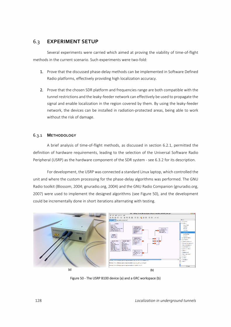
128 Localization in underground tunnels
6.3 EXPERIMENT SETUP
Several experiments were carried which aimed at proving the viability of time-of-flight
methods in the current scenario. Such experiments were two-fold:
1. Prove that the discussed phase-delay methods can be implemented in Software Defined
Radio platforms, effectively providing high localization accuracy.
2. Prove that the chosen SDR platform and frequencies range are both compatible with the
tunnel restrictions and the leaky-feeder network can effectively be used to propagate the
signal and enable localization in the region covered by them. By using the leaky-feeder
network, the devices can be installed in radiation-protected areas, being able to work
without the risk of damage.
6.3.1 METHODOLOGY
A brief analysis of time-of-flight methods, as discussed in section 6.2.1, permitted the
definition of hardware requirements, leading to the selection of the Universal Software Radio
Peripheral (USRP) as the hardware component of the SDR system - see 6.3.2 for its description.
For development, the USRP was connected a standard Linux laptop, which controlled the
unit and where the custom processing for the phase-delay algorithms was performed. The GNU
Radio toolkit (Blossom, 2004; gnuradio.org, 2004) and the GNU Radio Companion (gnuradio.org,
2007) were used to implement the designed algorithms (see Figure 50), and the development
could be incrementally done in short iterations alternating with testing.
(a)
(b)
Figure 50 - The USRP B100 device (a) and a GRC workspace (b)
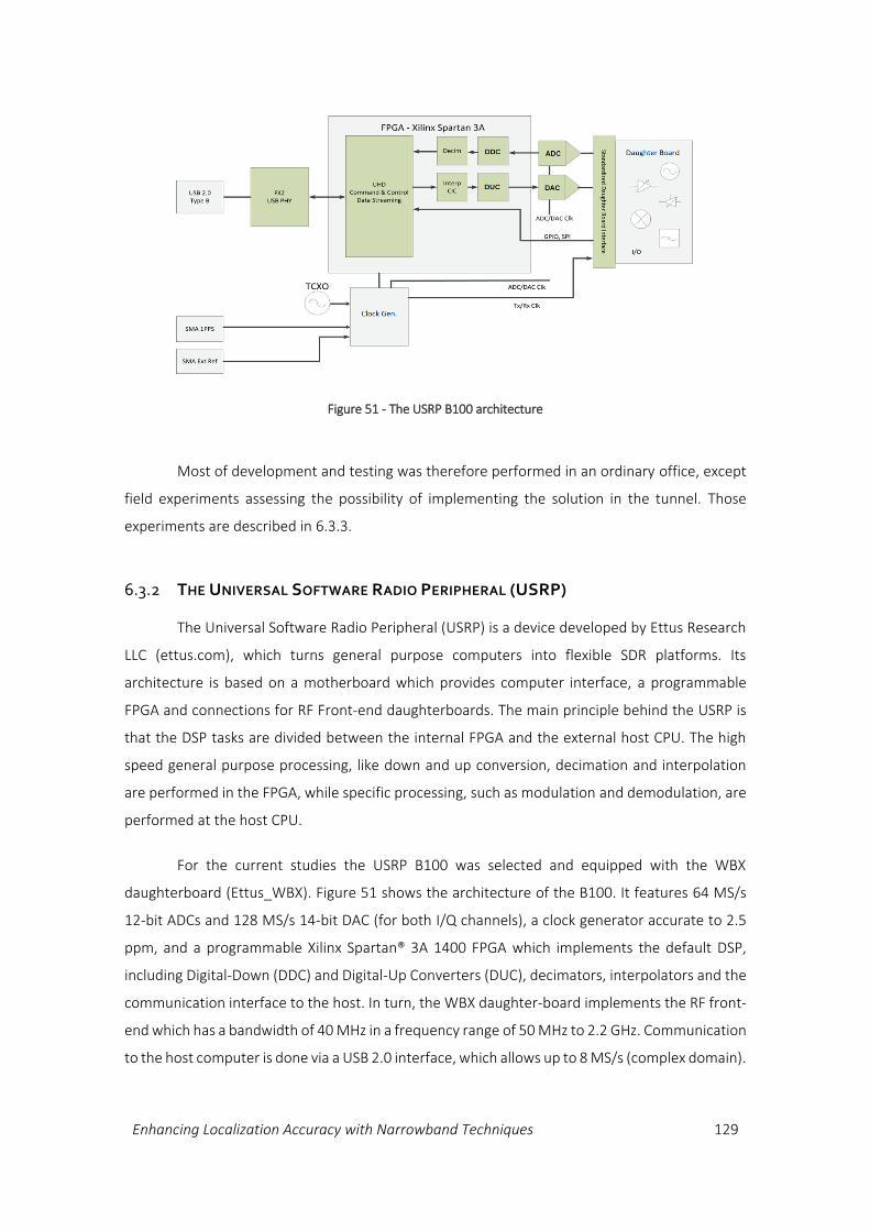
Enhancing Localization Accuracy with Narrowband Techniques 129
Most of development and testing was therefore performed in an ordinary office, except
field experiments assessing the possibility of implementing the solution in the tunnel. Those
experiments are described in 6.3.3.
6.3.2 THE UNIVERSAL SOFTWARE RADIO PERIPHERAL (USRP)
The Universal Software Radio Peripheral (USRP) is a device developed by Ettus Research
LLC (ettus.com), which turns general purpose computers into flexible SDR platforms. Its
architecture is based on a motherboard which provides computer interface, a programmable
FPGA and connections for RF Front-end daughterboards. The main principle behind the USRP is
that the DSP tasks are divided between the internal FPGA and the external host CPU. The high
speed general purpose processing, like down and up conversion, decimation and interpolation
are performed in the FPGA, while specific processing, such as modulation and demodulation, are
performed at the host CPU.
For the current studies the USRP B100 was selected and equipped with the WBX
daughterboard (Ettus_WBX). Figure 51 shows the architecture of the B100. It features 64 MS/s
12-bit ADCs and 128 MS/s 14-bit DAC (for both I/Q channels), a clock generator accurate to 2.5
ppm, and a programmable Xilinx Spartan® 3A 1400 FPGA which implements the default DSP,
including Digital-Down (DDC) and Digital-Up Converters (DUC), decimators, interpolators and the
communication interface to the host. In turn, the WBX daughter-board implements the RF front-
end which has a bandwidth of 40 MHz in a frequency range of 50 MHz to 2.2 GHz. Communication
to the host computer is done via a USB 2.0 interface, which allows up to 8 MS/s (complex domain).
Figure 51 - The USRP B100 architecture
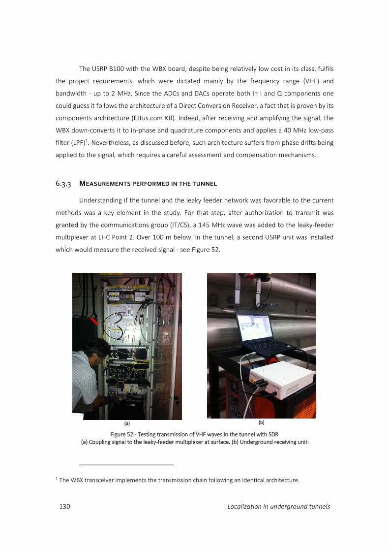
130 Localization in underground tunnels
The USRP B100 with the WBX board, despite being relatively low cost in its class, fulfils
the project requirements, which were dictated mainly by the frequency range (VHF) and
bandwidth - up to 2 MHz. Since the ADCs and DACs operate both in I and Q components one
could guess it follows the architecture of a Direct Conversion Receiver, a fact that is proven by its
components architecture (Ettus.com KB). Indeed, after receiving and amplifying the signal, the
WBX down-converts it to in-phase and quadrature components and applies a 40 MHz low-pass
filter (LPF)1. Nevertheless, as discussed before, such architecture suffers from phase drifts being
applied to the signal, which requires a careful assessment and compensation mechanisms.
6.3.3 MEASUREMENTS PERFORMED IN THE TUNNEL
Understanding if the tunnel and the leaky feeder network was favorable to the current
methods was a key element in the study. For that step, after authorization to transmit was
granted by the communications group (IT/CS), a 145 MHz wave was added to the leaky-feeder
multiplexer at LHC Point 2. Over 100 m below, in the tunnel, a second USRP unit was installed
which would measure the received signal - see Figure 52.
1 The WBX transceiver implements the transmission chain following an identical architecture.
(a)
(b)
Figure 52 - Testing transmission of VHF waves in the tunnel with SDR (a) Coupling signal to the leaky-feeder multiplexer at surface. (b) Underground receiving unit.
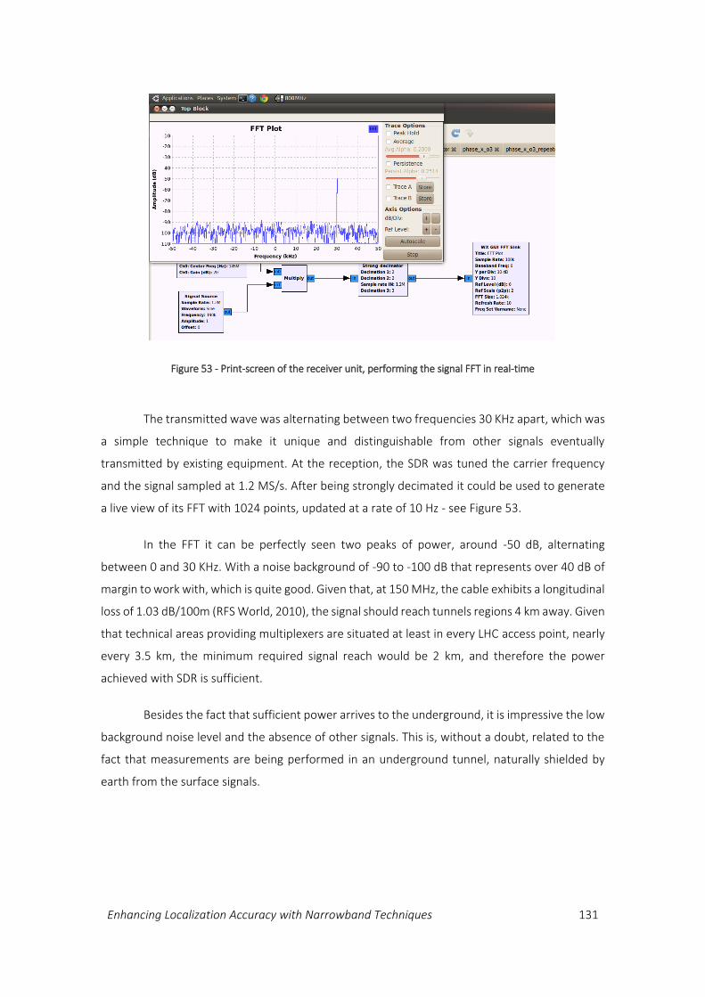
Enhancing Localization Accuracy with Narrowband Techniques 131
The transmitted wave was alternating between two frequencies 30 KHz apart, which was
a simple technique to make it unique and distinguishable from other signals eventually
transmitted by existing equipment. At the reception, the SDR was tuned the carrier frequency
and the signal sampled at 1.2 MS/s. After being strongly decimated it could be used to generate
a live view of its FFT with 1024 points, updated at a rate of 10 Hz - see Figure 53.
In the FFT it can be perfectly seen two peaks of power, around -50 dB, alternating
between 0 and 30 KHz. With a noise background of -90 to -100 dB that represents over 40 dB of
margin to work with, which is quite good. Given that, at 150 MHz, the cable exhibits a longitudinal
loss of 1.03 dB/100m (RFS World, 2010), the signal should reach tunnels regions 4 km away. Given
that technical areas providing multiplexers are situated at least in every LHC access point, nearly
every 3.5 km, the minimum required signal reach would be 2 km, and therefore the power
achieved with SDR is sufficient.
Besides the fact that sufficient power arrives to the underground, it is impressive the low
background noise level and the absence of other signals. This is, without a doubt, related to the
fact that measurements are being performed in an underground tunnel, naturally shielded by
earth from the surface signals.
Figure 53 - Print-screen of the receiver unit, performing the signal FFT in real-time
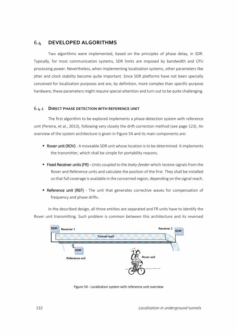
132 Localization in underground tunnels
6.4 DEVELOPED ALGORITHMS
Two algorithms were implemented, based on the principles of phase delay, in SDR.
Typically, for most communication systems, SDR limits are imposed by bandwidth and CPU
processing power. Nevertheless, when implementing localization systems, other parameters like
jitter and clock stability become quite important. Since SDR platforms have not been specially
conceived for localization purposes and are, by definition, more complex than specific-purpose
hardware, these parameters might require special attention and turn out to be quite challenging.
6.4.1 DIRECT PHASE DETECTION WITH REFERENCE UNIT
The first algorithm to be explored implements a phase-detection system with reference
unit (Pereira, et al., 2013), following very closely the drift-correction method (see page 123). An
overview of the system architecture is given in Figure 54 and its main components are:
Rover unit (ROV) - A moveable SDR unit whose location is to be determined. It implements
the transmitter, which shall be simple for portability reasons.
Fixed Receiver units (FR) - Units coupled to the leaky-feeder which receive signals from the
Rover and Reference units and calculate the position of the first. They shall be installed
so that full coverage is available in the concerned region, depending on the signal reach.
Reference unit (REF) - The unit that generates corrective waves for compensation of
frequency and phase drifts.
In the described design, all three entities are separated and FR units have to identify the
Rover unit transmitting. Such problem is common between this architecture and its reversed
Figure 54 - Localization system with reference unit overview
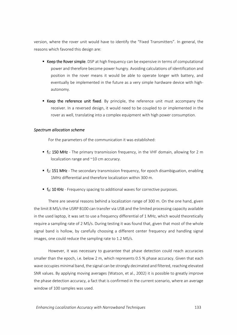
Enhancing Localization Accuracy with Narrowband Techniques 133
version, where the rover unit would have to identify the “Fixed Transmitters”. In general, the
reasons which favored this design are:
Keep the Rover simple. DSP at high frequency can be expensive in terms of computational
power and therefore become power hungry. Avoiding calculations of identification and
position in the rover means it would be able to operate longer with battery, and
eventually be implemented in the future as a very simple hardware device with high-
autonomy.
Keep the reference unit fixed. By principle, the reference unit must accompany the
receiver. In a reversed design, it would need to be coupled to or implemented in the
rover as well, translating into a complex equipment with high power consumption.
Spectrum allocation scheme
For the parameters of the communication it was established:
f1: 150 MHz - The primary transmission frequency, in the VHF domain, allowing for 2 m
localization range and ~10 cm accuracy.
f2: 151 MHz - The secondary transmission frequency, for epoch disambiguation, enabling
1MHz differential and therefore localization within 300 m.
fΔ: 10 KHz - Frequency spacing to additional waves for corrective purposes.
There are several reasons behind a localization range of 300 m. On the one hand, given
the limit 8 MS/s the USRP B100 can transfer via USB and the limited processing capacity available
in the used laptop, it was set to use a frequency differential of 1 MHz, which would theoretically
require a sampling rate of 2 MS/s. During testing it was found that, given that most of the whole
signal band is hollow, by carefully choosing a different center frequency and handling signal
images, one could reduce the sampling rate to 1.2 MS/s.
However, it was necessary to guarantee that phase detection could reach accuracies
smaller than the epoch, i.e. below 2 m, which represents 0.5 % phase accuracy. Given that each
wave occupies minimal band, the signal can be strongly decimated and filtered, reaching elevated
SNR values. By applying moving averages (Watson, et al., 2002) it is possible to greatly improve
the phase detection accuracy, a fact that is confirmed in the current scenario, where an average
window of 100 samples was used.

134 Localization in underground tunnels
Algorithm
As a prototype implementation, the configuration was simplified to a Rover (transmitter)
and a combined Receiver-Reference SDR unit. Considering the latter receives the two initial
frequencies, f1 and f1+fΔ, the challenge is exactly on the creation of a stable corrective wave.
Considering that the clock accuracy of USRP B100 is 2.5 ppm, and that the phase drift transfers
to base-band, we might face frequency drifts up to 2.5x150 (=375!) Hz. Despite the quite technical
background, the implementation is conceptually simple, the steps being:
1. Obtain fΔ’ as the difference between the phases of two incoming signals f1 and f1+fΔ
2. Obtain frΔ ‘ as the phase difference between the corrective fr and f1+fΔ.
3. Obtain fΔΔ as the phase difference between fΔ’ and frΔ ‘, which represents an error function
which must tend to zero.
4. Integrate the error function fΔΔ over time, so that a corrective delta function frΔ smoothly
converges.
5. Add phases of f1+fΔ and frΔ to obtain fr, the corrective wave.
In order to verify whether the algorithm is working properly, it is enough to monitor the
error function fΔΔ. When it converges and stabilizes at zero one knows that the delta signals are
equivalent and the system is accurately emitting the corrective waves.
SDR implementation
When working with signals defined by complex samples, in order to create a signal
representing the sum or difference of phases of two signals, the terms can be directly multiplied
(to obtain sum) or the first term multiplied with the conjugate of the second (for difference).
Given the existence of blocks implementing such functionalities in the GNU Radio
Companion (GRC) software, the previous algorithm might seem relatively straightforward to
implement. However, it was found that, due to the large margin for frequency drifts - up to 375
Hz - the system was taking too long to stabilize and, often, it would not stabilize before a new
drift occurred.

Enhancing Localization Accuracy with Narrowband Techniques 135
Due to that, a new design was investigated and implemented (Pereira, et al., 2013) which
aims at achieving faster stabilization - see Figure 55. The implementation makes use of three new
functional blocks (findMax, Running Integrator and Complex VCO) which had to be specifically
implemented in C++ for the purpose. It takes the FFT maximum of fΔΔ,, that is the frequency shift
between the signals fΔ’ and frΔ’, which is then passed to a running integrator, in order to converge
to the exact frequency of frΔ’. The frequency is then used by the complex VCO to create a wave in
that frequency, and phase fine-tuning is achieved by directly considering fΔΔ.
6.4.2 ROUND-TRIP PHASE DETECTION
In a round-trip setup, the signal is originally emitted and finally received by the same unit,
having a “reflection” unit in the middle. In such a design, the requirements for phase
compensation are relaxed, since both original and delayed signals are bound to the same clock
generator and therefore have perfect relative clock drift. For the current experiment the goal is
to verify whether, in SDR, the signal phase does not suffer from distortions in the transmission
and reception chains of both units and the phase-drifts applying in both directions of the same
device are counter-compensated.
Algorithm
Even though the round-trip method is conceptually straightforward, it incurs an
important difficulty: the wave can’t be directly reflected. Doing so, being a continuous wave, it
wouldn’t be possible to distinguish it from the loopback path, in which the signal travels directly
from the transmission to the reception circuits in the first unit. In order to tackle the problem it
is required to separate the flows. Since time separation is not an option, and code-multiplexing
would require the research of codes which would apply the same drift, two different frequencies
had to be used. However, different frequency shits are usually required in the units.
The key challenge behind such technique is to guarantee that any and every frequency
shift is applied forth and back by the same clock generator.
Figure 55 - Conceptual implementation of reference unit in direct phase detection
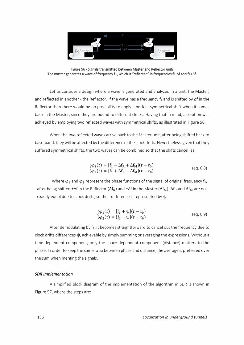
136 Localization in underground tunnels
Let us consider a design where a wave is generated and analyzed in a unit, the Master,
and reflected in another - the Reflector. If the wave has a frequency f1 and is shifted by Δf in the
Reflector then there would be no possibility to apply a perfect symmetrical shift when it comes
back in the Master, since they are bound to different clocks. Having that in mind, a solution was
achieved by employing two reflected waves with symmetrical shifts, as illustrated in Figure 56.
When the two reflected waves arrive back to the Master unit, after being shifted back to
base-band, they will be affected by the difference of the clock drifts. Nevertheless, given that they
suffered symmetrical shifts, the two waves can be combined so that the shifts cancel, as:
{φ1(𝑡) = [f1 − ΔfR + ΔfM](𝑡 − 𝑡0)
φ2(𝑡) = [f1 + ΔfR − ΔfM](𝑡 − 𝑡0) (eq. 6.8)
Where φ1 and φ2 represent the phase functions of the signal of original frequency f1,
after being shifted ±Δf in the Reflector (ΔfR) and ±Δf in the Master (ΔfM). ΔfR and ΔfM are not
exactly equal due to clock drifts, so their difference is represented by ψ.
{φ1(𝑡) = [f1 + ψ](𝑡 − 𝑡0)
φ2(𝑡) = [f1 − ψ](𝑡 − 𝑡0) (eq. 6.9)
After demodulating by f1, it becomes straightforward to cancel out the frequency due to
clock drifts differences ψ, achievable by simply summing or averaging the expressions. Without a
time-dependent component, only the space-dependent component (distance) matters to the
phase. In order to keep the same ratio between phase and distance, the average is preferred over
the sum when merging the signals.
SDR implementation
A simplified block diagram of the implementation of the algorithm in SDR is shown in
Figure 57, where the steps are:
Figure 56 - Signals transmitted between Master and Reflector units The master generates a wave of frequency f1, which is “reflected” in frequencies f1-Δf and f1+Δf.

Enhancing Localization Accuracy with Narrowband Techniques 137
1. A wave of frequency f1 is immediately sent out to air. The applied “shifts” are [f1M].
2. A second unit captures it (USRP source 2) and shifts it back to 0 Hz. Note: It is natural that
the wave is not exactly at 0 Hz due to the different clock drifts which affect both the
carrier frequency and the f1 demodulation frequency. Shifts: [f1M, -f1R].
3. The resulting wave is low-pass filtered and multiplexed into two frequencies f1-Δf and
f1+Δf. Shifts: [f1M, -f1R, f1R-ΔfR] and [f1M, -f1R, f1R+ΔfR] => [f1M, -ΔfR] and [f1M, +Δf R].
4. The initial unit receives the signals and shifts down from f1. Shifts: [f1M, -ΔfR, -f1M] and
[f1M, +ΔfR, -f1M]=> [-ΔfR] and [ΔfR].
5. The signals are independently shifted, down and up, by Δf. Shifts: [-ΔfR, ΔfM] and [+ΔfR, -
ΔfM] => [ψ] and [-ψ].
6. The signals have now perfectly opposite shift distortions. Since the absolute frequency
value shall be very small1, a moving average is applied for smoothing and finally the
average is taken to get the central constant value.
After an initial calibration at position 0, distance between the units will incur a signal
propagation delay measurable by a proportional phase shift. For reference, the diagram of the
full GRC implementation can be found in 0.
1 With a 2.5 ppm oscillator accuracy, a 10 KHz wave will have up to 2.5x0.01 (=0.025) Hz error.
Figure 57 - Conceptual implementation of the round-trip phase detection method
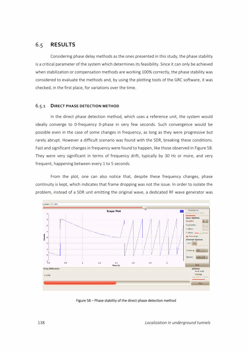
138 Localization in underground tunnels
6.5 RESULTS
Considering phase delay methods as the ones presented in this study, the phase stability
is a critical parameter of the system which determines its feasibility. Since it can only be achieved
when stabilization or compensation methods are working 100% correctly, the phase stability was
considered to evaluate the methods and, by using the plotting tools of the GRC software, it was
checked, in the first place, for variations over the time.
6.5.1 DIRECT PHASE DETECTION METHOD
In the direct phase detection method, which uses a reference unit, the system would
ideally converge to 0-frequency 0-phase in very few seconds. Such convergence would be
possible even in the case of some changes in frequency, as long as they were progressive but
rarely abrupt. However a difficult scenario was found with the SDR, breaking these conditions.
Fast and significant changes in frequency were found to happen, like those observed in Figure 58.
They were very significant in terms of frequency drift, typically by 30 Hz or more, and very
frequent, happening between every 1 to 5 seconds.
From the plot, one can also notice that, despite these frequency changes, phase
continuity is kept, which indicates that frame dropping was not the issue. In order to isolate the
problem, instead of a SDR unit emitting the original wave, a dedicated RF wave generator was
Figure 58 – Phase stability of the direct phase detection method
Enhancing Localization Accuracy with Narrowband Techniques 139
used. As a result the signal showed to be remarkably stable, eliminating the mentioned frequency
hopping phenomena almost completely. This fact strongly indicates that, at some point of the
transmit chain of the SDR, the signal suffers strong side effects which are not directly proportional
to the oscillator. This might be due to some components being highly sensitive to the clock
changes eventually at the level of the FPGA, or de-synchronisation happening among the
processing layers, introducing little frequency hops in the resulting wave.
Even considering the fast-convergence implementation of method, which needed a few
seconds to stabilize, such behaviour of the SDR reduced to zero the available time-window of
stable system and turned the method virtually helpless for localization in the current scenario.
Given the complexity of the SDR system, these issues represent a major obstacle whose
resolution is outside the scope of this thesis. Therefore alternative methods were investigated.
6.5.2 ROUND-TRIP METHOD
The second method, based on the round-trip principle to avoid clock synchronization
issues, was evaluated in a very similar way. After implementing the model, step-by-step tuning of
frequencies and filter parameters was performed and quite interesting results could be observed.
In the current setup, after being “reflected”, the signal could be recovered in the original
unit and, after being shifted to 0-frequency, it would behave well, without presenting any kind of
frequency hops – see Figure 59. Although sensitive to interference of nearby bodies, when
performed basic smoothing using a Moving Average filter, the phase would remain impressively
constant while perfectly responsive to distance changes.
Figure 59 – Phase stability of the round-trip method
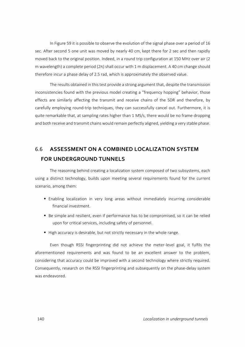
140 Localization in underground tunnels
In Figure 59 it is possible to observe the evolution of the signal phase over a period of 16
sec. After second 5 one unit was moved by nearly 40 cm, kept there for 2 sec and then rapidly
moved back to the original position. Indeed, in a round trip configuration at 150 MHz over air (2
m wavelength) a complete period (2π) shall occur with 1 m displacement. A 40 cm change should
therefore incur a phase delay of 2.5 rad, which is approximately the observed value.
The results obtained in this test provide a strong argument that, despite the transmission
inconsistencies found with the previous model creating a “frequency hopping” behavior, those
effects are similarly affecting the transmit and receive chains of the SDR and therefore, by
carefully employing round-trip techniques, they can successfully cancel out. Furthermore, it is
quite remarkable that, at sampling rates higher than 1 MS/s, there would be no frame dropping
and both receive and transmit chains would remain perfectly aligned, yielding a very stable phase.
6.6 ASSESSMENT ON A COMBINED LOCALIZATION SYSTEM
FOR UNDERGROUND TUNNELS
The reasoning behind creating a localization system composed of two subsystems, each
using a distinct technology, builds upon meeting several requirements found for the current
scenario, among them:
Enabling localization in very long areas without immediately incurring considerable
financial investment.
Be simple and resilient, even if performance has to be compromised, so it can be relied
upon for critical services, including safety of personnel.
High accuracy is desirable, but not strictly necessary in the whole range.
Even though RSSI fingerprinting did not achieve the meter-level goal, it fulfils the
aforementioned requirements and was found to be an excellent answer to the problem,
considering that accuracy could be improved with a second technology where strictly required.
Consequently, research on the RSSI fingerprinting and subsequently on the phase-delay system
was endeavored.
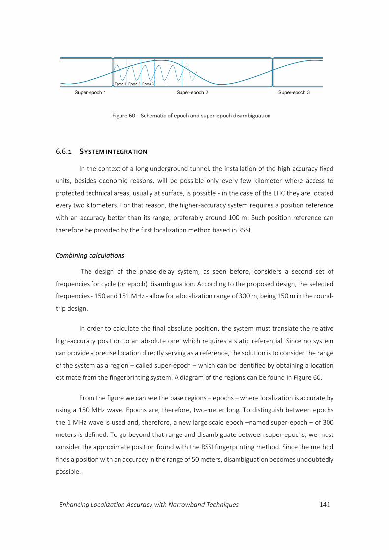
Enhancing Localization Accuracy with Narrowband Techniques 141
6.6.1 SYSTEM INTEGRATION
In the context of a long underground tunnel, the installation of the high accuracy fixed
units, besides economic reasons, will be possible only every few kilometer where access to
protected technical areas, usually at surface, is possible - in the case of the LHC they are located
every two kilometers. For that reason, the higher-accuracy system requires a position reference
with an accuracy better than its range, preferably around 100 m. Such position reference can
therefore be provided by the first localization method based in RSSI.
Combining calculations
The design of the phase-delay system, as seen before, considers a second set of
frequencies for cycle (or epoch) disambiguation. According to the proposed design, the selected
frequencies - 150 and 151 MHz - allow for a localization range of 300 m, being 150 m in the round-
trip design.
In order to calculate the final absolute position, the system must translate the relative
high-accuracy position to an absolute one, which requires a static referential. Since no system
can provide a precise location directly serving as a reference, the solution is to consider the range
of the system as a region – called super-epoch – which can be identified by obtaining a location
estimate from the fingerprinting system. A diagram of the regions can be found in Figure 60.
From the figure we can see the base regions – epochs – where localization is accurate by
using a 150 MHz wave. Epochs are, therefore, two-meter long. To distinguish between epochs
the 1 MHz wave is used and, therefore, a new large scale epoch –named super-epoch – of 300
meters is defined. To go beyond that range and disambiguate between super-epochs, we must
consider the approximate position found with the RSSI fingerprinting method. Since the method
finds a position with an accuracy in the range of 50 meters, disambiguation becomes undoubtedly
possible.
Figure 60 – Schematic of epoch and super-epoch disambiguation
142 Localization in underground tunnels
As an example, let us consider that the system is aligned to the metrical marking of the
tunnel, so that at position 0 m we have phase 0 in both phase-measurement systems, and the
case of using the system and obtain the readings: π/2 rad for the 150 MHz wave, 3π/2 rad for the
1 MHz one, and an absolute metrical position of 2060±50 m from the fingerprinting method.
Translating the distance to epochs, one finds that the location should be between super-epoch 7
(at 70% of its length or 210m) and super-epoch 8 (at 10 m relative to the beginning). A
measurement of 3π/2, which translates to 225 m (3/4 of 300 m), lies undoubtedly in the region
selected by the first method and helps confirming we are in super-epoch 7. The same principle
applies to the next stage. Knowing that 3π/2 is 75% of the length, we end up in the middle of the
epoch 113 (300*0.75/2). A measurement of π/2 rad for the 150 MHz wave represents 0.5 m (25%
of 2 m). The final position is therefore given by (7-1)x300 + (113-1)x2 + 0.5 = 2024.5m (±10 cm
considering a phase accuracy of 5% at 150 MHz).
Physical integration
Despite being two independent technologies, the need for combining results from both
systems motivates the development of an integrated unit. Moreover, factors as the relatively
simplicity of both methods, the high performance of programmable hardware – including FPGAs,
and concerns on power-consumption, strongly favor an implementation further integrated into
a single combined unit.
Even though an analysis on the implementation of the system is outside the scope of this
thesis, a potential architecture is mentioned for the purpose of better illustrating applications. In
an integrated design, the Rover must implement receivers in the GSM, WLAN and VHF band,
transmitters in VHF and a GPRS communication module to transmit the location. Besides the
Rover, Transmitters and Reference units are required in the areas where high-accuracy is
intended.
6.6.2 ADVANTAGES OF MODULARITY
Despite the fact that the combination of systems was necessary, there are several
advantages from such a modular architecture. Having both systems decoupled makes each one
simpler and less prone to problems. Furthermore, there is a considerable improvement with
respect to flexibility, as it can be better customized to applications having different needs,
eventually requiring a single localization technology.
Enhancing Localization Accuracy with Narrowband Techniques 143
A summary of the advantages, from a System and User perspectives, is given below.
System perspective
Simplicity – Each component is less complex and can be developed independently.
Robustness – Each component is simpler and therefore more robust. The inherent
robustness of the fingerprinting-based system is saved which is especially important to
make it suitable for safety and rescue purposes.
Flexibility – Depending on the application, low-accuracy in a long range or high accuracy
in a short range can be independently employed as well, translating into cost-effective
solutions.
User perspective
Cost-effectiveness – Besides solutions comprising a single system, the long-range coarse
localization system can be progressively upgraded to high-accuracy in areas where it is
justified.
Higher-Availability – in case of maintenance of the high-accuracy system, eventually more
common given its higher degree of complexity, lower-accuracy localization and
dependent processes, especially critical ones, shall not be affected.
6.6.3 APPLICABILITY - POSSIBLE USE CASES
The researched solution targets the case of the LHC tunnel which, despite representing
a rather unique environment housing a particle accelerator, has requirements that can surely be
found in many other situations. To recapitulate (from Table 2, page 49) some of the key target
characteristics:
Accuracy: regularly 10-50 m, up to 1 m in special areas.
Range: tens of kilometers (27 in the case of the LHC).
Output data: 1D position.
High availability (>95%) and Robustness.
Infrastructure: no devices shall be installed in the area.
Cost: relatively low, upgradeable.

144 Localization in underground tunnels
Such characteristics are easily found in mines and other tunnels where hazardous
activities are carried out. Especially in those cases, where emergency management and rescue
are extremely important activities, there haven’t been solutions that respect the required
robustness while enabling for high-accuracy where required.
Despite being designed for radioactive and hazardous tunnels, the developed solution is
a highly promising answer to many other scenarios:
Road tunnels – Long roadway tunnels, which are commonly used to transverse mountain
regions, typically dispose a radio communication infrastructure using leaky-feeder, and
therefore localization could be introduce with minimal cost.
Building connection paths and city undergrounds – In some industrial complexes and cities,
where underground tunnels connect buildings or are used for telecom, power and
sewage services, localization might be of extreme importance for e.g. safety purposes.
In order to meet harsh conditions, like dirt and humidity, a solution based on a single
radiating cable might be among the best and only possibilities.
Tracking of important objects in logistic centers, airports and industrial lines – Considering
complex logistic routes for, e.g., goods in a logistic center, luggage in airports, products
in a factory, it is conceivable to deploy a radiating cable along the lines. By installing
receivers on important objects, they can be tracked so that their routing is guaranteed,
avoiding loss and meeting the best delivery timings.
In turn, a localization system uniquely having a high accuracy-component, even though it
was not designed with such objectives, can also be of interest in diverse situations, including:
Tracking in corridors – Whereas people or moveable objects are to be tracked or informed
of its position, a single phase-delay system can provide an accurate tag in a relatively
long section, up to 300m. Instead of using leaky-feeder, such a system can be composed
of units emitting RF to air directly.
Industrial alignment – Considering a hall or corridor where pieces of machinery or
equipment are to be installed at relatively precise places, fixed units can be attached to
a wall and distance can be obtained with the rover units. By employing a second set of
fixed units in a perpendicular wall, 2-D coordinates might be achieved for wide spaces.
Enhancing Localization Accuracy with Narrowband Techniques 145
6.6.4 SCIENTIFIC VALUE
Even though leaky-feeders are commonly found in mines and tunnels, maybe due to the
low attenuation levels found with such cables, no underground localization solution was found to
take advantage of GSM or even proprietary signals by using fingerprinting. In the current research
work it was found that, despite the limitations, such methods yield reasonable accuracy which is
suitable for safety purposes and to serve higher accuracy methods by identifying a region.
One of the major knowledge advances yielding from the current study is the proof that,
even under very tight budgets and engineering resources, it is possible to deploy large scale
localization systems that even comply with challenging scenarios and retrofit in existing
installations. To date and to the knowledge of the author, there is not any hardware device
capable of performing fingerprinting which is flexible enough to work with a range of network
technologies and eventually to allow for selecting radio-frequency within a considerable band.
The implementation of such a device, despite conceptually simple, could be a significant
milestone in providing localization services in scenarios which had never been considered before.
Furthermore, the possibility of enhancing the accuracy where necessary by installing fixed
hardware units is a novel concept which brings more flexibility and increases possibilities and cost
control.
A slight discovery originating in the current research work was the verification that signals
propagating in the same direction in a leaky-feeder cable will exhibit a remarkably identical power
profile – see section 4.2.4. Unfortunately, such phenomena didn’t occur in signals propagating in
opposite directions, which prevented the ICRD method from yielding better results.
As a last point, even though less significant, we believe that the thorough investigation
of the background theoretical concepts from dozens of sources allowed the author to compile
the relevant subjects in a condensed yet comprehensive and logically-structured way.
146 Localization in underground tunnels
6.7 CONCLUSIONS
This chapter presented the studies on localization techniques for accurate positioning in
the CERN tunnels, and its feasibility using Software-Defined-Radio (SDR) platforms. Two
narrowband approaches, based on the principle of Time-of-Flight, were investigated. On the one
hand, one approach uses direct-phase detection with a synchronization signal, requiring very
simple Rover units. On the other hand, a round-trip approach relaxes the need for
synchronization but requires the clock shifts to be perfectly symmetrical. Moreover clock jitter
and frame-dropping must stay within acceptable limits.
Tests using the USRP B100 and GNU Radio showed that the first approach could not
achieve the expected behavior since the signal was recurrently being affected by fast frequency
shifts which could not be compensated within the available time frame. In turn, the round-trip
approach showed to perform quite well, as the effects introduced in the signal along the transmit
chain of the SDR were cancelled out when also passing through the receive chain of the same
device. Relative movement of the units among each other could therefore be perfectly
observable, as the measured phase change correctly represented the displacement.
In the last part of the chapter, an analysis of the complete system if performed. Being
composed of two sub-systems, the proposed solution has inherent advantages from both the
development and end-user perspectives, like simplicity, robustness and added flexibility, making
it valuable for different scenarios including safety in tunnel roadways and city undergrounds,
tracking of objects in logistic centers and airports, and alignment in industrial contexts.
Conclusions 147
Chapter 7
CONCLUSIONS
This thesis presents the research on localization techniques targeting a very unique
underground environment - the accelerator tunnels at CERN, specifically that hosting the Large
Hadron Collider (LHC). The specific nature of these tunnels where bulky metallic equipment and
panels are present, together with the ambitious goal of providing high accuracy localization in an
environment with very rigid and restrictive deployment regulations for equipment, were the
foundation of a singular problem. This unique setting presented an exciting challenge which had
to be tackled.
Despite the existence of extensive literature for indoors localization, there’s very little
research on underground localization not requiring specific infrastructure, the most relevant
publications investigating WLAN over leaky-feeders in a short tunnel section. Building on the same
idea, several experiments were conducted in the current tunnel in order to characterize and
exploit the existing signals, namely GSM and WLAN, for localization purposes. The detailed
characterization of the signals received power (RSSI), presented in Chapter 4, shows that the
attenuation of the GSM signal, despite being in tight agreement with the cable specification
(around 3 dB/100m), suffer from significant variations. Discrepant values, up to 10 dB, are found
for the same point among different measurement sessions or slightly different measurement
conditions. Indeed, when there was somebody nearby or the distance between the cable and the
antenna changed, the RSSI would considerably be affected, up to 20dBs in the latter case. It was
also verified that the RSSI could increase or decrease non-uniformly in subsequent measurement
points, a situation where analytical method become particularly ineffective. In a more detailed
scan, in which a third GSM channel was detected, it was found that the power profile among the
two channels propagating in the same direction was very similar, with a spearman rank-order
coefficient up to 99%. When carrying out experiments with WLAN, in a setup involving two access
points installed 150 m apart, it was verified that the longitudinal attenuation is much higher, in
the order of 14 dB/100m, and RSSI differences among the several sessions much smaller, typically
less than 3 dB - a condition that is expected to favor localization.

148 Localization in underground tunnels
Considering that the measurement could be performed in reasonably similar conditions,
and that each position is, to some degree, unique, empirical methods show up as an attractive
yet simply approach for localization. RSSI fingerprinting methods are explored in
Chapter 5, with several KNN variants in different configurations being tested. With GSM it was
verified that, under optimal conditions, i.e., when the measurements belong to the same session,
NN could yield exceptional results, finding the correct point 86% of the cases. However, under
more realistic conditions, i.e., when obtaining the online fingerprint from another session, the
values drastically drop reaching the same probability only with KNN, K=5 and an error-distance of
80 m – these two cases can be graphically viewed in plots E and F from Appendix C. In order to
improve on these performance figures, several approaches were explored. Among the most
significant, by merging the radio-map from several sessions one can reduce the error-distance to
60 m, and if one can further merge the online fingerprints the error-distance gets as low as 40 m
at 90% confidence. In another plane, a new weighting method to KNN was developed, which
attempts to consider the reliability of a measurement from its standard deviation. The results are
very positive, and show an improvement in the whole error-distance domain, up to 27% (both
cases using a merged radio-map). Furthermore, by taking advantage of channels power
differential, the ICRD method was developed which doesn’t consider the absolute power
anymore. Therefore, despite exhibiting similar performance, it is expected to reduce the need for
calibration. Moreover, to better understand the limitations, an ideal KNN was modeled and tested
with GSM. It was found that the exact match is very often not within the K selected results and
therefore, to further improve the accuracy, more sources of information would be required.
Tests with WLAN revealed much more expressive results. Without optimizations, it can
achieve 30 m of distance-error in 91% of the cases. Consequently, a multi-technology method
was developed to take advantage of the several available signals. Tests with GSM and WLAN
together revealed that the performance would just be coincident as with WLAN alone, as they
unfortunately exhibited very different performance levels. However, the deployment of WLAN in
the LHC is only possible during extended maintenance periods, since off-the-shelf APs would
suffer permanent damage if exposed to the radiation of a high-energy accelerator in operation.
Given the impossibility of further improving the accuracy with RSSI fingerprinting
methods, a complementary system, based on the principles of TOF, was investigated. Meeting
the tunnel restrictions and leveraging the existing VHF network, a phase-delay measurement
system with synchronization units was developed and considered as a second stage of the
localization where high-accuracy is required. From the implementation in SDR one could learn
Conclusions 149
that frequency shifts, stemming from its Direct Conversion Receiver architecture, occur
frequently, making synchronization between units extremely difficult. A second approach,
following the radar principle, is then explored and an algorithm for counter-compensating
random phase-shifts is developed. The approach proves to work well even with SDR devices and
displacements among the units can be precisely measured.
As a solution being composed of two sub-systems, it shows advantages from both the
system and end-user perspectives, including simplicity, robustness and added flexibility. Besides
its application in the challenging environment of a particle accelerator tunnel, the technology is
shown useful in many other contexts, like safety in tunnel roadways, tracking of objects in logistic
centers and airports, and alignment in industrial halls.
THESIS CONTRIBUTION AND ACHIEVEMENTS
The RSSI fingerprinting and phase-delay systems, even though they were tested
separately and are in an investigation state, were conceived to work together. RSSI fingerprinting
was proved to work sufficiently well for coarse localization, with accuracy around 50 m, which
would enable for safety purposes, including finding people in case of emergency. The fact that
the system is totally passive and uses GSM which is considered a safety system with fail-safe
mechanisms, makes it very robust and ideal for safety. In areas where accurate localization would
be needed or worth the investment, the second level of localization could be enabled by installing
the necessary equipment in the respective surface cell. Even though the joint high accuracy
system could not be experimentally tested in the tunnel due to reasons of access limitation, the
experiments support the validity of the theoretical model and therefore a careful integration,
especially if implemented in dedicated hardware, would achieve the desired outcome.
Besides serving as a solid basis for a possible implementation in the LHC tunnel, this thesis
presents an important contribution to the understanding of the signal properties and localization
in harsh tunnel environments. Among the main topics, (1) the characterization of the signal
propagating over leaky-feeder, (2) the power profile analysis and observation of the ICRD
properties, (3) the development of KNN variants in a generic location fingerprinting framework
and (4) the design and development of an high-accuracy localization system using Software
Defined Radio developed knowledge (including IT tools) which is expected to be an important
reference for new studies and localization systems in similar underground environments, where
the existing or eventually undisclosed information is virtually inexistent.

150 Localization in underground tunnels
FUTURE WORK
Even though the concepts developed in this thesis were thoroughly analyzed and tested,
there’s a wide range of possibilities where further advances could be investigated and
implemented. In the first place, RSSI fingerprinting methods could be explored with filtering
techniques, e.g. employing Kalman or Particle filters. Even though preliminary studies in that
direction were made, the results didn’t yield the desirable performance gains, sufficient to avoid
a secondary system. Furthermore, given that those methods are already well-known in literature
they were not further investigated in the context of this thesis. Regarding the phase-delay system,
further development could be done in order to allow for communication between the Rover and
Fixed units or even among Rovers, which would allow to share the location with, e.g., the central.
From the perspective of implementation, despite not directly related to a PhD work,
there are a number of challenges that would need to be tackled by a team of software and
hardware engineers. For instance, to improve the sending and receiving of signal via a single
medium – the leaky-feeder – and avoid saturation of the receive chain, it is important to reduce
the feedback loop. Circulators are a technology that can be employed for the purpose and could
be tested in the existing scenario. Also, the Rover unit would eventually work best as a combined
GSM and VHF transceiver with a control module implemented in, e.g., an FPGA. As so, efficient
power consumption and high portability would be possible while avoiding the limitations of SDR,
while the combined logic would take care of determining the “sector” using RSSI fingerprinting
and, where available, use the high accuracy infrastructure to find the precise location.
FINAL WORDS
Location techniques, in particular those based in fingerprinting, are a hot research topic
nowadays. A lot of investigation has been put towards the application of these methods to the
most diverse areas while improving their accuracy. Location finding has become ubiquitous,
serving the most diverse areas, from game-playing to disaster management.
The development of this thesis work, and specially its writing, besides the additional
knowledge it might have brought to academia, was an experience with profound repercussions
to the author’s scientific and personal mindset. Perseverance was probably one of the most
crucial attitudes developed throughout the work and which was sustained by two pillars: the
motivation of contributing to such an extraordinary field, and the people who helped creating the
beautiful research environments I took part in.
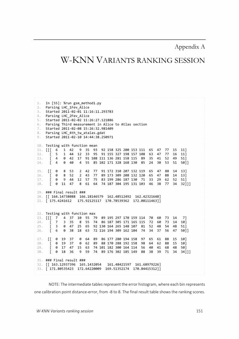
W-KNN Variants ranking session 151
Appendix A
W-KNN VARIANTS RANKING SESSION
NOTE: The intermediate tables represent the error histogram, where each bin represents
one calibration point distance-error, from -8 to 8. The final result table shows the ranking scores.
1. In [55]: %run gsm_method1.py 2. Parsing LHC_1Fev_Alice 3. Started 2011-02-01 11:16:11.293783 4. Parsing LHC_2Fev_Alice 5. Started 2011-02-02 11:26:27.121886 6. Parsing Third measurement in Alice to Atlas section 7. Started 2011-02-08 15:26:32.981409 8. Parsing LHC_4th_tw_atalas.gdat 9. Started 2011-02-10 14:44:38.250971 10. Testing with function mean 11. [[[ 6 1 42 9 35 93 92 158 325 200 153 111 65 47 77 15 11] 12. [ 5 1 44 12 33 95 91 155 327 198 157 108 63 47 77 16 11] 13. [ 4 0 42 17 91 108 111 136 281 158 115 89 35 41 52 49 51] 14. [ 4 0 40 4 55 85 102 171 328 168 130 85 24 30 53 51 50]] 15. [[ 0 8 53 2 42 77 91 172 310 207 132 119 65 47 88 14 13] 16. [ 0 8 52 2 43 77 89 173 309 208 132 120 65 47 88 14 13] 17. [ 0 9 44 12 57 75 83 199 286 187 130 71 33 29 62 52 51] 18. [ 0 11 47 8 61 64 74 187 304 195 131 103 46 38 77 34 32]]] 19. ### Final result ### 20. [[ 164.14738088 166.18146579 162.48512492 162.42321648] 21. [ 175.4241612 175.92125117 170.78539362 172.08111463]] 22. Testing with function max 23. [[[ 7 4 37 10 55 79 89 195 297 170 159 114 70 60 73 14 7] 24. [ 7 3 35 8 55 74 86 187 305 171 165 115 72 60 73 14 10] 25. [ 3 0 47 25 65 92 130 164 265 148 107 81 52 48 54 48 51] 26. [ 6 0 38 18 63 72 116 194 309 162 104 74 34 37 56 47 50]] 27. [[ 0 19 37 0 64 89 86 177 280 194 158 97 65 61 88 15 10] 28. [ 0 19 37 0 62 89 88 170 288 192 158 98 64 62 88 15 10] 29. [ 0 17 47 15 63 74 101 182 300 164 114 56 40 41 68 48 50] 30. [ 0 18 36 9 59 74 89 176 302 185 149 88 38 39 71 34 34]]] 31. ### Final result ### 32. [[ 163.12937396 165.1432054 161.48421597 161.68979226] 33. [ 171.80535423 172.64220009 169.51352174 170.84415312]]

152 Localization in underground tunnels
(This page was intentionally left blank)

Score to relative function 153
Appendix B
SCORE TO RELATIVE FUNCTION
1. def score_to_relative( results, weights=None ): 2. """ Calculate the relative (inc cumulative) scores of a result set. 3. Weights can be provided to be applied to the relative result 4. """ 5. assert weights is None or len(weights) == len(results), “Size mimatch” 6. 7. tot = .0 8. parts = [] 9. for i,resu in enumerate(results): 10. value = float(resu[1]) if resu[1]>.1 else 0.1 #Avoid div by 0 11. weight = float(weights[i]) if weights is not None else 1.0 12. part = (1.0+weight)/value 13. parts.append( part ) 14. tot += part 15. 16. out = [] 17. cumulative = .0 18. for i,resu in enumerate(results): 19. rel_score = parts[i] / tot 20. cumulative += rel_score 21. out.append( resu + [ rel_score, cumulative ] ) 22. 23. return sorted( out, key=lambda x: x[2], reverse=True )

154 Localization in underground tunnels
Appendix C
W-KNN EXPERIMENTAL RESULTS
NOTE: “None” is used to represent fingerprint or mobile merging.
Selecting only those whose statistical function is the mean and using merged mobiles, we
end up with 8 accuracy plots, from where we can exclude those whose fingerprints are
considered independently, i.e. [1,2]. The accuracy plots are shown next.
In: nl.average_accuracy() Out: [ Radio-MAP Fingerprints Mobiles Stat Func Avg. Accuracy ] [PLOT]
1. [(None, [None], [1, 2], 'mean', 75.000000000), 2. (None, [None], [1, 2], 'median', 74.568965517), 3. (None, [None], [None], 'mean', 87.643678160), A 4. (None, [None], [None], 'median', 87.643678160), 5. (None, [1], [1, 2], 'mean', 67.959770114), 6. (None, [1], [1, 2], 'median', 66.810344827), 7. (None, [1], [None], 'mean', 68.965517241), B 8. (None, [1], [None], 'median', 69.540229885), 9. (None, [2], [1, 2], 'mean', 59.770114942), 10. (None, [2], [1, 2], 'median', 60.775862068), 11. (None, [2], [None], 'mean', 60.632183908), C 12. (None, [2], [None], 'median', 58.333333333), 13. (None, [1, 2], [1, 2], 'mean', 63.864942528), 14. (None, [1, 2], [1, 2], 'median', 63.793103448), 15. (None, [1, 2], [None], 'mean', 64.798850574), 16. (None, [1, 2], [None], 'median', 63.936781609), 17. (1, [None], [1, 2], 'mean', 57.327586206), 18. (1, [None], [1, 2], 'median', 59.195402298), 19. (1, [None], [None], 'mean', 60.632183908), D 20. (1, [None], [None], 'median', 59.482758620), 21. (1, [1], [1, 2], 'mean', 74.712643678), 22. (1, [1], [1, 2], 'median', 77.729885057), 23. (1, [1], [None], 'mean', 89.367816091), E 24. (1, [1], [None], 'median', 91.091954022), 25. (1, [2], [1, 2], 'mean', 54.454022988), 26. (1, [2], [1, 2], 'median', 53.591954022), 27. (1, [2], [None], 'mean', 49.425287356), F 28. (1, [2], [None], 'median', 48.563218390), 29. (1, [1, 2], [1, 2], 'mean', 64.583333333), 30. (1, [1, 2], [1, 2], 'median', 65.660919540), 31. (1, [1, 2], [None], 'mean', 69.396551724), 32. (1, [1, 2], [None], 'median', 69.827586206) ]
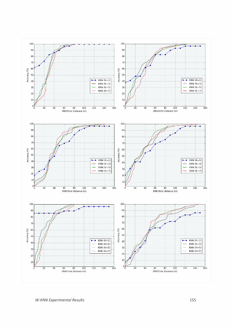
W-KNN Experimental Results 155
A B
C D
E F

156 Localization in underground tunnels
(This page was intentionally left blank)

Round-trip method implementation in GNU-Radio Companion 157
Appendix D
ROUND-TRIP METHOD IMPLEMENTATION IN
GNU-RADIO COMPANION
Figure 61 – Implementation of the round-trip method

158 Localization in underground tunnels
(This page was intentionally left blank)
Bibliography 159
BIBLIOGRAPHY
Akyildiz, I. F., Sun, Z. & Vuran, M. C., 2009. Signal propagation techniques for wireless underground communication networks. Physical Communication, Volume 2, pp. 167-183.
Ali-Loytty, S., Sirola, N. & Piche, R., 2005. Consistency of Three Kalman Filter Extensions in Hybrid Navigation. Munich, Proceedings of the European Navigation Conference GNSS 2005.
Ávila Rodríguez, J., 2011. GPS Signal Plan. [Online] Available at: http://www.navipedia.net/index.php/GPS_Signal_Plan
Bahl, P. & Padmanabhan, V., 2000. RADAR: an in-building RF-based user location and tracking system. INFOCOM 2000. Nineteenth Annual Joint Conference of the IEEE Computer and Communications Societies. Proceedings. IEEE, Volume 2, pp. 775-784.
Bandyopadhyay, L. K. et al., 2010. Mine-Wide Communication. pp. 121-140.
Barrett, C., 1999. Fractional/Integer-N PLL Basics, Dallas, US: Texas Instruments - Wireless Communication Business Unit.
Beder, C., McGibney, A. & Klepal, M., 2011. Predicting the expected accuracy for fingerprinting based WiFi localisation systems. Guimarães, Indoor Positioning and Indoor Navigation (IPIN 2011), Proceedings of.
Bensky, A., 2007. Wireless positioning technologies and applications. London: Artech House.
Blossom, E., 2004. GNU Radio: Tools for Exploring the Radio Frequency Spectrum. Linux Journal, 2004(122).
Castro, P., Chiu, P., Kremenek, T. & Muntz, R., 2001. A Probabilistic Room Location Service for Wireless Networked Environments. Atlanta, 3rd International Conference on Ubiquitous Computing (Ubicomp 2001).
Cerda, R. M., 2005. Understanding TCXOs. Microwave Product Digest, April, p. 42.
CERN, 2008. CERN - The Large Hadron Collider. [Online] Available at: http://public.web.cern.ch/public/en/LHC/LHC-en.html
CERN, 2014. About CERN. [Online] Available at: http://public.web.cern.ch/public/en/About/About-en.html [Accessed 2014].
160 Localization in underground tunnels
Cheng, Y. C., Chawathe, Y. & Krumm, J., 2005. Accuracy characterization for metropolitan-scale Wi-Fi localization. Technical Report IRS-TR-05-003 ed. s.l.:Intel Research.
Chiba, J. et al., 1978. Radio communication in tunnels. Microwave Theory and Techniques, IEEE Transactions on, Volume 26, pp. 439--443.
Chon, H. D., Jun, S., Jung, H. & An, S. W., 2004. Using RFID for Accurate Positioning. Journal of Global Positioning Systems, 3(1-2), pp. 32-39.
Čihař, M., online. Gammu. [Online] Available at: http://wammu.eu/gammu/ [Accessed 2010].
Dayekh, S., Affes, S., Kandil, N. & Nerguizian, C., 2011. Cooperative geo-location in underground mines: A novel fingerprint positioning technique exploiting spatio-temporal diversity. s.l., Proceedings of PIMRC pp.1319-1324.
Delogne, P., 1991. EM propagation in tunnels. Antennas and Propagation, IEEE Transactions, March, Volume 39, pp. 401 -406.
Denby, B., Oussar, Y., Ahriz, I. & Dreyfus, G., 2009. High-Performance Indoor Localization with Full-Band GSM Fingerprints. Dresden, s.n., pp. 1 -5.
Drane, C., Macnaughtan, M. & Scott, C., 1998. Positioning GSM telephones. IEEE Communications Magazine, 36(4), pp. 45-59.
Duda, R. O., Hart, P. E. & Stork, D. G., 2000. Pattern Classification. 2nd ed. s.l.:Wiley-Interscience.
EC, 2002. Directive on privacy and electronic communications, European Commission, Tech. Rep: 2002/58/EC.
Engelbrecht, J., Collmann, R., Birkel, U. & Weber, M., 2010. Methodical leaky feeder design for indoor positioning considering multipath environments. New York, Radio and wireless symposium (RWS).
Engelbrecht, J., Collmann, R., Birkel, U. & Weber, M., 2011. First results of a leaky coaxial cable prototype for indoor positioning. New York, Wireless telecommunications symposium.
Engelbrecht, J., Forster, G., Michler, O. & Collmann, R., 2012. Positioning estimation in public transport systems by leaky coaxial cables. Dresden, 9th workshop on positioning navigation and communication (WPNC).
Erceg, V. et al., 1999. An empirically based path loss model for wireless channels in suburban. IEEE Journal on Selected Areas in Communications, 17(7), pp. 1205-1211.
Ettus.com KB, n.d. Bandwidth Capability of USRP Devices. [Online] Available at: http://www.ettus.com/kb/detail/usrp-bandwidth

Bibliography 161
ettus.com, n.d. Ettus Research LLC. [Online] Available at: http://www.ettus.com/
Ettus_WBX, n.d. WBX-40 50 MHz - 2.2 GHz Rx/Tx. [Online] Available at: http://www.ettus.com/product/details/WBX
Fang, L. et al., 2005. Design of a wireless assisted pedestrian dead reckoning system - the NavMote experience. Instrumentation and Measurement, IEEE Transactions on, 54(6), pp. 2342 - 2358 .
FCC, 1996. Revision of the Commission Rule to ensure compatibility with enhanced 911 emergency calling system, Federal Communications Commission, Tech. Rep.: RM-8143 Washington, DC.
Figueiras, J. & Frattasi, S., 2010. Mobile Positiong and Tracking. s.l.:Wiley.
Fink, A., Beikirch, H., Voss, M. & Schroder, C., 2010. RSSI-based indoor positioning using diversity and Inertial Navigation. Zurich, Indoor Positioning and Indoor Navigation (IPIN), 2010 International Conference on.
Frigge, M., Hoaglin, D. C. & Iglewicz, B., 1989. Some Implementations of the Boxplot. The American Statistician, Feb, 43(1), pp. 50-54.
Gadeke, T., Schmid, J., Stork, W. & Muller-Glaser, K. D., 2011. Pedestrian Dead Reckoning for Person Localization in a Wireless Sensor Network. Guimarães, Indoor Positioning and Indoor Navigation (IPIN), 2011 International Conference on.
Gardiner, C., 1985. Handbook of Stochastic Methods for Physics, Chemistry and the Natural Sciences. Berlin: Springer-Verlag.
Gezici, S. et al., 2005. Localization via ultra-wideband radios. Signal Processing Magazine, IEEE, july, Volume 22, pp. 70 - 84.
gnuradio.org, 2004. GNU Radio official website. [Online] Available at: http://gnuradio.org/redmine/projects/gnuradio/wiki [Accessed 2013].
gnuradio.org, 2007. GNU Radio Companion. [Online] Available at: http://gnuradio.org/redmine/projects/gnuradio/wiki/GNURadioCompanion [Accessed 2013].
Goldsmith, A., 2005. Wireless Communications. s.l.:Cambridge University Press.
Goyal, P., Ribeiro, V. J., Saran, H. & Kumar, A., 2001. Strap-down Pedestrian Dead-Reckoning system. Guimarães, Indoor Positioning and Indoor Navigation (IPIN), 2011 International Conference on.
GPS joint program office, 2004. Navstar GPS Space Segment/Navigation User Interfaces. [Online] Available at: http://www.losangeles.af.mil/shared/media/document/AFD-070803-059.pdf
162 Localization in underground tunnels
GPS.gov, 2014. The Global Positioning System. [Online] Available at: http://www.gps.gov/systems/gps/ [Accessed 2014].
Grewal, M. & Andrews, A., 2001. Kalman Filter: Theory and Practice Using MATLAB. 2nd ed. s.l.:Wiley & Sons.
Haeberlen, A. et al., 2004. Practical robust localization over large-scale 802.11 wireless networks. Philadelphia, USA, Proceedings of the 10th Annual International Conference on Mobile Computing and Networking.
Honkavirta, V., 2008. Location fingerprinting methods in wireless local area networks, Ms.C thesis: Tampere University of Technology.
Honkavirta, V., Perala, T., Ali-Loytty, S. & Piche, R., 2009. A Comparative Survey of WLAN Location Fingerprinting Methods. Positioning, Navigation and Communication, 6th Workshop on, IEEE, pp. 243-251.
Hopper, A., Harter, A. & Blackie, T., 1993. The active badge system. s.l., ACM, pp. 533--534.
IEEE, 1997. IEEE Standard for Information Technology Part 11: Wireless LAN Medium Access Control (MAC) and Physical Layer (PHY) Specifications. IEEE Std 802.11-1997.
IEEE, 2009. IEEE Standard for Information Technology Part 11: Wireless LAN Medium Access Control (MAC) and Physical Layer (PHY) Specifications Amendment 5: Enhancements for Higher Throughput. IEEE Std 802.11n-2009.
InfraSurvey, 2013. InfraSurveys UGPS3. [Online] Available at: http://www.infrasurvey.ch/en/products/ugps3 [Accessed 2013].
Isomäki, P. & Avessta, N., 2004. An Overview of Software Defined Radio Technologies, Turku, Finland: TUCS Laboratory.
Julier, S. & Uhlmann, J., 1997. A new extension of the Kalman filter to nonlinear systems. Orlando, USA, International Symposium on Aerospace/Defense Sensing, Simulation and Controls.
Jung, P., Bruck, G., Waadt, A. & Wang, S., 2009. An apparatus and method operative for providing traffic information on a traffic area. Germany, Patent No. EP2287820 A1.
Kaemarungsi, K., 2006. Distribution of WLAN received signal strength indication for indoor location determination, Tech. Rep: National Electronics and Computer Technology Center, Thailand.
Kaemarungsi, K. & Krishnamurthy, P., 2004. Modeling of indoor positioning systems based on location fingerprinting. INFOCOM 2004. Twenty-third AnnualJoint Conference of the IEEE Computer and Communications Societies, Volume 2, pp. 1012-1022.
Kailath, T., Sayed, A. & Hassibi, B., 2000. Linear Estimation. s.l.:Prentice Hall.
Bibliography 163
Kalman, R., 1960. A new approach to linear filtering and prediction problems. Journal of Basic Engineering, 82(1), pp. 35-45.
Langley, R. B., 1991. The mathematics of GPS. GPS world, 2(7), pp. 45-50.
Latvala, J., Syrjärinne, J., Ikonen, H. & Niittylahti, J., 2000. Evaluation of RSSI-based human tracking. Proc. 2000 European Signal Processing Conference, Volume 4, p. 2273–2276.
Li, B., Salter, J., Dempster, A. G. & Rizos, C., 2006. Indoor positioning techniques based on wireless LAN, Technical report: School of Surveying and Spatial Information Systems, UNSW, Sydney, Australia.
Linnartz, J. P., 1993. Cellular Telephone Networks. [Online] Available at: http://www.wirelesscommunication.nl/reference/chaptr04/cellplan/cellsize.htm [Accessed Oct. 2014].
Lin, T.-N. & Lin, P.-C., 2005. Performance comparison of indoor positioning techniques based on location fingerprinting in wireless networks. Wireless Networks, Communications and Mobile Computing, 2005 International Conference on, Volume 2, pp. 1569-1574.
Mahalanobis & Chandra, P., 1936. On the generalised distance in statistics. Proceedings of the National Institute of Sciences of India, 2(1), pp. 49-55.
Marconi, 1909. Wireless Telegraphic Communication, Amsterdam: Nobel Lectures Physics, Elsevier.
Mautz, R., 2012. Indoor Positioning Technologies, s.l.: [Hab thesis] ETH Zurich.
Michalson, W. R. & Progri, I. F., 2000. Assessing the accuracy of underground positioning using pseudolites, ION GPS-2000: Technical Meeting of Institute of Navigation.
Misra, P., Jha, S., Ostry, D. & Kottege, N., 2011. An Envelope Detection based Broadband Ultrasonic Ranging System for Improved Indoor/Outdoor Positioning, UNSW-CSE-TR-1106: University of New South Wales.
Mitola, J., 1995. The Software Radio Architecture. IEEE Communications Magazine, 33(5), pp. 26-38.
Nakamura, M. et al., 2010. Development of a simple multiple-position identifying system with a long range multiband leaky coaxial cable for rescue operations in tunnels or passages in underground facilities. Yokohama, Microwave Conference Proceedings (APMC), 2010 Asia-Pacific.
Nebot, E. M., 1999. Sensors Used for Autonomous Navigation. In: Advances in Intelligent Autonomous Systems. s.l.:Springer, pp. 135-156.
Novak, T., Snyder, D. P. & Kohler, J. L., 2010. Postaccident Mine Communications and Tracking Systems. Industry Applications, IEEE Transactions on, Volume 46, pp. 712--719.
Otsason, V., Varshavsky, A., LaMarca, A. & de Lara, E., 2005. Accurate GSM indoor localization. LNCS, Springer, p. 141–158.

164 Localization in underground tunnels
Parsons, J. D., 2000. The Mobile Radio Propagation Channel. 2nd ed. s.l.:Wiley.
Pereira, F., Theis, C., Cunha, S. R. & Ricardo, M., 2013. Accurate positioning in underground tunnels using Software-Defined-Radio. Montbeliard, France, Indoor Positioning and Indoor Navigation (IPIN), 2013 International Conference on, pp. 196-201.
Pereira, F., Theis, C., Moreira, A. & Ricardo, M., 2011. Evaluating Location Fingerprinting Methods for Underground GSM Networks deployed over Leaky Feeder. Guimarães, Portugal, Indoor Positioning and Indoor Navigation (IPIN), 2011 International Conference.
Pereira, F., Theis, C., Moreira, A. & Ricardo, M., 2012. Multi-technology RF fingerprinting with leaky-feeder in underground tunnels. Sydney, Australia, Indoor Positioning and Indoor Navigation (IPIN), 2012 International Conference on.
Prasithsangaree, P., Krishnamurthy, P. & Chrysanthis, P., 2002. On indoor position location with wireless LANs, PA 15260, Tech. Rep.: Telecommunications Program, University of Pittsburgh.
Priyantha, N. B., Chakraborty, A. & Balakrishnan, H., 2000. The Cricket location-support system. s.l., ACM, pp. 32--43.
Randell, C., Djiallis, C. & Muller, H., 2003. Personal position measurement using dead reckoning. s.l., Wearable Computers, IEEE Proceedings.
Rappaport, T. S., 1996. Wireless Communications Principles and Practice. s.l.:Prentice Hall.
Reed, J. H., 2002. RF Receiver Front-End Topologies. In: Software Radio: A Modern Approach to Radio Engineering. s.l.:Prentice Hall.
RFS World, 2010. 1-1/4" RADIAFLEX® RLKW Cable, A-series. [Online] Available at: http://www.rfsworld.com/dataxpress/Datasheets/?q=RLKW114-50JFLA
Roos, T. et al., 2002. A probabilistic approach to wlan user location estimation. International Journal of Wireless Information Networks, 9(3), pp. 155-163.
Schneider, O., 2010. Indoor Positioning and Indoor Navigation (IPIN), 2010 International Conference on. Zurich, CH, Requirements for positioning and navigation in underground constructions.
SDR Forum, 1999. TECHNICAL REPORT 2.1: Architecture and Elements of Software Defined Radio Systems as Related to Standards, s.l.: s.n.
U.S. Naval Research Laboratory, 1943. Monopulse Radar. [Online] Available at: http://www.nrl.navy.mil/accomplishments/systems/monopulse-radar/
US Naval Observatory, 2000. USNO NAVSTAR Global Positioning System. [Online] Available at: http://tycho.usno.navy.mil/gpsinfo.html
Valerio, D., 2008. Open Source Software-Defined Radio: A survey on GNUradio and its applications, Vienna: s.n.
Bibliography 165
Varshavsky, A. et al., 2006. Are GSM Phones THE Solution for Localization?. s.l., s.n., pp. 20 - 28.
Viegas, D., 2005. Sound Wave Phase Processing for Precise Positioning, MsC thesis, s.l.: Faculdade de Engenharia da Universidade do Porto.
Vossiek, M. et al., 2003. Wireless local positioning. IEEE Microwave Magazine, Volume 4, pp. 77-86.
Ward, A., Jones, A. & Hopper, A., 1997. A New Location Technique for the Active Office. IEEE Personal Communications, Volume 4, pp. 42--47.
Watson, S. et al., 2002. Frequency downconversion and phase noise in MIT. Physiological Measurement, 23(1), p. 189.
Weber, M., Birkel, U. & Collmann, R., 2009. Indoor RF Fingerprinting using leaky feeder cable considering environmental changes. s.l., s.n., pp. 1--6.
Weber, M., Birkel, U., Collmann, R. & Engelbrech, J., 2011. Wireless indoor positioning : Localization improvements with a leaky coaxial cable prototype. Guimaraes, Portugal, Indoor Positioning and Indoor Navigation 2011, pp. 21-23.
Weber, M., Birkel, U., Collmann, R. & Engelbrecht, J., 2010. Comparison of various methods for indoor RF fingerprinting using leaky feeder cable. New York, 7th workshop on positioning navigation and communication (WPNC).
Yamaguchi, Y., Abe, T., Sekiguchi, T. & Chiba, J., 1985. Attenuation Constants of UHF Radio Waves in Arched Tunnels (Short Paper). Microwave Theory and Techniques, IEEE Transactions on, Volume 33, pp. 714--718.
Yenchek, M. R., n.d. Through-the Earth Mine Communication Systems, Presentation: Office of mine safety and health research, Pittsburgh.
Youssef, M. A., Agrawala, A., Shankar, A. U. & Noh, S. H., 2002. A Probabilistic Clustering-Based Indoor Location Determination System, Technical Report CS-TR-4350 and UMIACS-TR-2002-30: University of Maryland.
Zhou, J., Yeung, W. M. & Ng, J. K., 2008. Enhancing Indoor Positioning Accuracy by utilizing signals from both the mobile phone network and the Wireless Local Area Network. s.l., s.n., pp. 138--145.