Positioning Inventory in Clinical Trial Supply Chains

October 20, 2012

Abstract

As a result of slow patient recruitment and high patient costs in the United States, clini-

cal trials are increasingly going global. While recruitment efforts benefit from a larger global

footprint, the supply chain has to work harder at getting the right drug supply, to the right

place, at the right time. Certain clinical trial supply chains, especially those supplying biologics,

have a combination of unique attributes that have yet to be addressed by existing supply chain

models. These attributes include a fixed patient horizon, an inflexible supply process, a unique

set of service-level requirements, and an inability to transfer drug supplies among testing sites.

In this paper, we provide a new class of multi-echelon inventory models to address these unique

aspects. The resulting mathematical program is a nonlinear integer programming problem with

chance constraints. Despite this complexity, we develop a solution method that transforms the

original formulation into a linear integer equivalent. By analyzing special cases and numerically

studying a hypothetical real-life example, we develop novel insights into inventory positioning

in clinical trial supply chains. We also study the impact of site network on the supply chain

cost and the trade-off between inventory overage and the expected recruitment time.

Keywords and Phrases: Clinical trial supply chain, multi-echelon inventory model, finite

patient horizon.

1 Introduction

Clinical trials, as mandated by the United States Food and Drug Administration (FDA), seek to

test the safety and efficacy of an investigative drug in human subjects. Given the drug’s absence

of an established safety record, potential patients are understandably leery of enrolling in these

trials. In the United States, these patients tend to favor already approved treatment options. Not

surprisingly, patient recruitment is a typical bottleneck in conducting clinical trials and one study

suggests that 80% of clinical trials are failing to meet their patient recruitment deadlines (Getz and

de Bruin 2000). To counter the slow patient recruitment and high costs of enrolling patients in

the United States, clinical trials are increasingly going global in their search for patients (Rowland

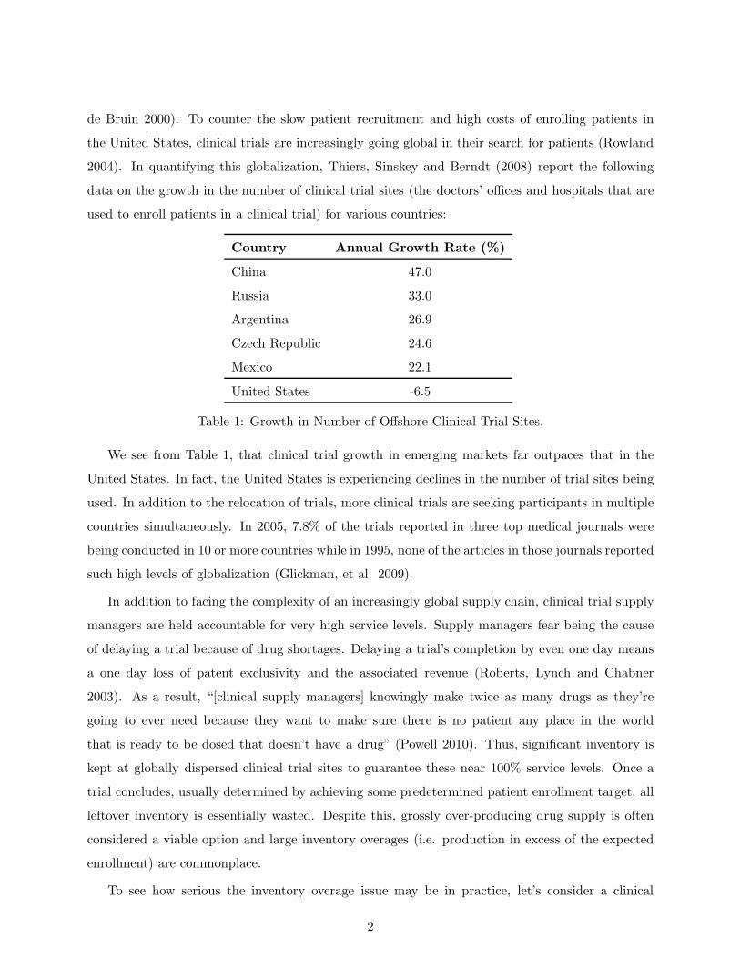
2004). In quantifying this globalization, Thiers, Sinskey and Berndt (2008) report the following

data on the growth in the number of clinical trial sites (the doctors’ offices and hospitals that are

used to enroll patients in a clinical trial) for various countries:

Country Annual Growth Rate (%)

China 47.0

Russia 33.0

Argentina 26.9

Czech Republic 24.6

Mexico 22.1

United States -6.5

Table 1: Growth in Number of Offshore Clinical Trial Sites.

We see from Table 1, that clinical trial growth in emerging markets far outpaces that in the

United States. In fact, the United States is experiencing declines in the number of trial sites being

used. In addition to the relocation of trials, more clinical trials are seeking participants in multiple

countries simultaneously. In 2005, 7.8% of the trials reported in three top medical journals were

being conducted in 10 or more countries while in 1995, none of the articles in those journals reported

such high levels of globalization (Glickman, et al. 2009).

In addition to facing the complexity of an increasingly global supply chain, clinical trial supply

managers are held accountable for very high service levels. Supply managers fear being the cause

of delaying a trial because of drug shortages. Delaying a trial’s completion by even one day means

a one day loss of patent exclusivity and the associated revenue (Roberts, Lynch and Chabner

2003). As a result, “[clinical supply managers] knowingly make twice as many drugs as they’re

going to ever need because they want to make sure there is no patient any place in the world

that is ready to be dosed that doesn’t have a drug” (Powell 2010). Thus, significant inventory is

kept at globally dispersed clinical trial sites to guarantee these near 100% service levels. Once a

trial concludes, usually determined by achieving some predetermined patient enrollment target, all

leftover inventory is essentially wasted. Despite this, grossly over-producing drug supply is often

considered a viable option and large inventory overages (i.e. production in excess of the expected

enrollment) are commonplace.

To see how serious the inventory overage issue may be in practice, let’s consider a clinical

2

trial which plans to enroll 612 patients (this example is stylized from the 612-patient, 45-site trial

described in Le Chevalier, et al. 1994). If there is only one site, shipping 612 drug kits to the site

ensures a 100% fill rate. To accelerate patient recruiting, 45 sites can be opened, but imposing

a typical 99% fill rate for the first 612 patients requires shipping 1035 kits to the sites (assuming

inventory is carried only at sites and patient recruitment follows a Poisson process with independent

but identical arrival rates at all sites). The planned overage is 423 kits, about 70% of the required

kits.

Recently, huge overages are being scrutinized. Clinical supply managers are being asked to

cut costs as clinical supply costs can potentially account for a significant portion (e.g., 40%, see

Fleischhacker 2009 for examples) of the clinical trial spending. With large pharmaceutical compa-

nies like Bristol Meyers Squibb spending roughly $200 million per year on clinical supplies, they

estimate that reducing planned overages is a way to save $40 million annually (Powell 2010). As

eroding pharmaceutical profits are a fact of life for the industry, reducing overages is a logical

response to budgetary pressures; the goal of the clinical supply manager is to do more with less.

Patrick Vallance, Senior Vice President - Medicines Discovery and Development at GlaxoSmithK-

line (GSK), describes GSK’s migration away from using large inventory overages in clinical trials

(Vallance 2011):

Four years ago, it was the norm when ordering clinical trial supplies to have an overage

of over 100% sometimes 200%. Statistical and mathematical modeling show that you

can reduce that overage to under 50%... [Using those modeling tools, our overages went]

from an average of well over 100% [in 2006] to something under 50% [in 2009] resulting

in $120 million of drug substance savings. This late-stage focus on these efficiencies is

incredibly important when running these large clinical studies.

As suggested in the above quote, mathematical models are becoming instrumental tools to

support the inventory needs of global trials on tighter budgets. Yet despite this, very little modeling

(other than simulation) that accommodates the unique elements of clinical trial supply chains is

available in academic or practitioner literature. The question of how to manage inventory to

efficiently support a global clinical trial is largely unanswered. In this paper, we study a class of

clinical trial supply chains and address their unique requirement by a new class of multi-echelon

inventory models.

3

1.1 Clinical Trial Supply Chain – An Example

For large global clinical studies, clinical trial supply chains are highly complex and no two clinical

trials are run in exactly the same manner. We present disguised details of a trial that a large U.S.

based pharmaceutical company conducted and for which relevant data has been provided. The trial

tested the effectiveness of an antibiotic in treating a specific type of infection and may be deemed

typical for Phase III testing of biologic drugs. The trial’s patient horizon (i.e. the target number

of patients to be recruited) was 600 and the patient recruitment was accomplished in nine months.

During the trial, each patient received one clinical trial package (i.e. drug supply, packaging,

and labeling) and all treatments were administered intravenously in a hospital or doctor’s office.

Previously collected drug stability data supported a 24-month shelf life for the investigational drug

and thus, drug expiration was not a concern for this trial.

The supply chain for this trial started with active pharmaceutical ingredient (API) production,

formulation and packaging, all completed in Europe. Distribution from the central warehouse in

Italy to 32 trial sites world-wide was accomplished via multiple country depots. Using country

depots is typical and Alex Klim (2010) of DHL Supply Chain’s Clinical Trial Logistics Service

succinctly states the reasoning as applied when shipping to Brazil, Russia, India and China (BRIC):

... the vast majority of large and medium sized pharmaceutical manufacturers and

biotechs still like to manufacture their research and development (R&D) products in

their European and North American production plants. This invariably means apply-

ing for an import license and having to go through the BRIC country’s importation

processes to supply a local depot. Although it is not completely impossible to operate

without it, it is highly advisable to have a local depot to store bulk medical supplies

in each of the BRIC countries; this is largely due to the long lead times around the

importation process, or in some cases due to local regulations.

Transit times from central warehouse to country depots were on the order of a few weeks, consisting

mainly of regulatory clearance time as opposed to actual transportation time. Transit times from

depots to sites were on the order of a few days.

Traditionally, inventory of investigative drugs is often held at trial sites to account for the

requirements of recruited patients without much resupply from the depots and central warehouse

(Peterson, Byrom, Dowlman, McEntegart 2004). An alternative is to pull back some inventory to

the depots and central warehouse, and resupply the sites as needed. The question is, how should

4

we position inventory in the clinical trial supply chain to ensure the desired drug availability in the

most cost efficient manner? To answer this question, we must account for the unique features of

clinical trial supply chains.

1.2 Clinical Trial Supply Chains – Unique Features

Clinical trial supply chains resemble spare part supply chains; they have similar network structure

and each seeks to satisfy demand that is random, infrequent1, and only met at the lowest echelon

of the supply chain. However, clinical trial supply chains require new mathematical models due to

many unique attributes:

• A Finite Patient Horizon, S: Each clinical trial has a predefined recruitment target, S, which

is the necessary sample size for the study. S is part of a protocol that is specified prior to

trial commencement and deviations from the protocol will jeopardize the acceptance of trial

results by the FDA. Once the target is reached, recruitment is closed and no more patients

will be enrolled in the trial. 2

• Inflexible Supply: Due to statistical consistency considerations and/or the significant fixed

costs associated with the production and quality control of investigational drugs, companies

often produce once for the entire trial prior to its commencement. This is particularly true for

biologics that are produced using biology-based processes (as opposed to chemical processes)

such as vaccines and many cancer therapies. For biologic trials, only a very small number of

production lots can be used so that statistical consistency, in regards to efficacy and safety of

the different lots, can be maintained. For example, Pederson et al (2007) study the effective-

ness of a human papillomarvirus vaccine by randomizing patients to receive drug supply from

one of four specific production lots. All lots were manufactured prior to administering the

vaccine in any trial participants. In addition, with the regulatory and testing requirements

imposed by the FDA, it is considered desirable, when possible, to have a drug of uniform

quality that was produced all in one batch or in one run (see Oncolytics Biotech 2003 for an

example).

• Inability of Cross-Shipping: By regulation, site-to-site shipping is discouraged and must “re-

main the exception” due to possible safety and trial quality issues (European Commission

1As described in §6, the anticipated enrollment rate at any one site is often much less than one patient per day.2Since the safety and efficacy of the drug are being tested, it makes sense to cease new exposures to the drug until

results are evaluated.

5

2003). In Andrews’ (2004) analysis of the strategic value of clinical supplies, he notes that

“in practice, the delays and potential for mistakes in retrieving a batch of material from one

site and re-releasing and/or transferring to another can, and does, make this course of action

impractical.” In fact, study sponsors often impose “standard operating procedures [which]

prohibit the transfer of study drug from one site to another.” (Barnett International 2010).

Cross shipping from one country depot to another country depot is also not recommended

because of customs issues, the need for relabeling, and potential risks of disqualifying a trial

due to poor regulatory adherence regarding drug accountability.

• Two Stringent Service-Level Requirements: A clinical trial supply chain manager is tasked

with achieving high immediate fill rates at sites and an even higher patient fill rate

for the entire trial. The immediate fill rate measures the percentage of patients at a site

who are administered the investigative drug immediately upon arrival. The patient fill rate

measures the percentage of patients entering the trial who are eventually administered the

drug. In other words, the patient fill rate measures the percentage of patients rejected from

the trial because the corresponding sites run out of stock and the system exhausts all inventory

available to resupply the sites.

Because a rejection of a patient or a delay of service due to clinical drug shortages is considered

unacceptable, the system must have sufficient inventory for the first S (the sample size)

patients regardless of which site they arrive to, and it is also desirable that drug supply is

immediately available to those patients. In practice, the trial is designed to achieve a patient

fill rate of 100% or nearly 100%, and very high immediate fill rates (often exceeding 99%).

The 100% patient fill rate ensures that each site can continue recruiting patients until the

patient enrollment target is reached and thus, minimizes the recruitment time. Practitioners

often adopt these service level requirements as a proxy for their time-to-market performance

because estimating the cost of time is difficult due to uncertainties in the trial outcome, the

drug’s market potential, and the opportunity cost of time and money not being available to

support investment in another drug’s clinical trial.

These unique attributes, combined with a complex logistics network, inherent demand uncer-

tainty (due to random enrollments at sites and randomization of patients), and relatively high

shipping costs, make a global clinical-trial supply chain difficult to manage. In absence of more

sophisticated modeling techniques, companies produce multiples of baseline forecasts as planned

overage (McDonnell and Mooraj 2009). However, this overage is essentially a costly waste that

6

ultimately leads to paying for the destruction of expensive materials. Clearly, the initial inventory

position in the system can have a significant impact on the overage and service levels due to the

inability of cross-shipping among sites and country depots. Thus, one of the main challenges in the

clinical trial supply chain is to achieve the required service levels with the minimum supply chain

cost by making intelligent inventory decisions.

1.3 Summary of Results

In this paper, we investigate the inventory decisions made within clinical trial supply chains. Specif-

ically, we determine the optimal upfront production quantity, the optimal inventory positions, and

the optimal shipping quantities to minimize the system-wide inventory overage and shipping costs

while achieving the desired immediate fill rates at the sites and the desired patient fill rate for the

trial (§1.2).We first present a new class of multi-echelon inventory models incorporating the unique aspects

of the clinical trial supply chain. We then develop a solution method that transforms the non-

linear integer programming problem with chance constraints to a linear integer equivalent. The

transformation relies on one of the unique aspects of clinical trial supply chains, the “finite patient

horizon”, to generate a “finite” set of deterministic constraints equivalent to the stochastic chance

constraints. The transformation can be done in a pseudo-polynomial time in the patient horizon

and shipping quantities. By analyzing a few special cases and numerically studying a hypothetical

real-world example, we show that the optimal stock positions in clinical trial supply chains differ

qualitatively from the classical multi-echelon inventory literature and the tradition in practice, and

thus can lead to significant savings. Finally, we study the impact of site network on supply chain

costs and also, the trade-off between the planned inventory overage and the expected recruitment

time.

2 Literature Review

A good introduction to the challenges of managing a global clinical trial supply chain can be found

in Lis, Gourley, Wilson, and Page (2009) where it is succinctly noted that “the key challenge clinical

trial supply chain (CTSC) managers face in global distribution is ensuring that supplies arrive at

the trial sites on time and in good condition.” To be on time, the inventory not only must be

produced in sufficient quantity to meet demand, but must also be properly positioned in the supply

7

chain to satisfy demand as it is realized.

The management of inventory in these supply chains has attracted limited attention from in-

dustry, and has attracted even less attention from academia. In industry literature, it is usually

advocated that inventory control policies in the clinical trial supply chain are selected using sim-

ulation (see Abdelkafi, Beck, David, Druck and Horoho 2009 and Peterson, Byrom, Dowlman and

McEntegart 2004 and references therein). In contrast, this is the first paper that we know of to

present an analytical model for inventory control in clinical trial supply chains. While analytic

models generally have the drawbacks of simplifying assumptions, the assumptions we make here

are typical and consistent with our motivating example. Some notable similarities and differences

between our model and simulation studies include:

• Dosage Level Changes: In some trials, various patients may be assigned to different dosing

levels of the investigational drug and the dosage levels being tested may change over the

course of the trial. This is an example of an adaptive trial and would be atypical, but

supported by simulation. Most trials are still traditional with dosage being set prior to

the trial starting. Our motivating example and analytical model are consistent with the

traditional trial approach.

• Continuous Review Inventory Policy: It is often assumed within these simulation models that

an integrated voice response system (IVRS) is available so that inventory can be monitored

continuously in time (McEntegar and O’Gorman 2005) and as inventory at a location falls

below a specified trigger, more inventory is ordered. Our paper also adopts this assumption.

• Inventory Policy as Model Output: The output of our model is an inventory policy for a given

set of service levels. In contrast, simulation studies require the inventory policy as input and

then simulate the service level performance. Thus, prior to deciding an inventory policy,

simulation models require multiple combinations of inventory policies to be tested with each

one requiring multiple (in the thousands) Monte Carlo simulations to ensure compliance with

the near 100% service levels as required by clinical trials.

• Perishability: Unlike our motivating example where shelf-life is not an issue, many clinical

trials must deal with the issue of perishability. We recognize that simulation is better equipped

at handling shelf-life concerns and that analytic modeling of inventory systems with perishable

products often require “analysis of multidimensional stochastic processes, and fairly involved

computations, due to the rapid growth of dimensionality of the process under investigation.”

8

(Ravichandran 1995)

Despite the availability of sophisticated tools for simulation in the real-world, inventory policies

(e.g., the trigger levels, shipping quantities) in clinical trial supply chains are still often set using

experience and by looking at the patterns from previous clinical trials. Going forward, we can

envision that both analytic models and simulation models will be used with more frequency. In

fact, it is highly desirable to combine the two by using analytic models to generate initial input

for simulation models when more detailed modeling assumptions are required (software tools like

BioClinica Optimizer also advocate this combined approach).

Sophisticated models have been developed to manage inventory in distribution networks (e.g.,

for spare parts). However, these models have yet to find their way to the problems faced by clinical

trials and yet, it is noted that these models are needed. Shah (2004) points out many of the key

challenges faced by pharmaceutical supply chains and surveys the literature that addresses those

challenges. Of particular interest is the recent focus of academicians on capacity planning for clinical

trial supply. Our work differs from this surveyed work in that we assume the allocation of capacity

to support a trial has already taken place and we now focus on the more operational/tactical policy

details of managing trial inventory.

Within the context of multiechelon inventory research, our models are most closely related

to work done for service parts where inventory is reviewed continuously in time (see reviews by

Zipkin 2000, Muckstadt 2005 and Simchi-Levi and Zhao 2011). One seminal work in this stream

of literature is Sherbrooke (1968). He approximated the distribution of backorders at the depot

by its first moment in a two-echelon distribution system when one-for-one ordering policies are

used. Improving on this approximation is the two-moment approximation by Graves (1985) who

shows how to effectively approximate backorder and lead time demand by a negative binomial

distribution. Svoronos and Zipkin (1991) refine the approximation by Graves (1985) and extend it

to evaluate multi-echelon distribution systems.

Graves (1985) and Axsater (1990) provide means to exactly evaluate the distribution of net

inventory levels in a multi-echelon distribution system, but these methods require the convolution

of multiple probability distributions and thus are computationally intensive. Simchi-Levi and Zhao

(2005) extend the exact approach to evaluate tree structure supply chains subject to fill rate

constraints, but in making the stock positioning decisions, approximations in line with Graves

(1985) and Svoronos and Zipkin (1991) are utilized.

All aforementioned work focuses on one-for-one ordering policies. Batch ordering policies, which

9

account for economies of scale, also received considerable attention in the literature. Zipkin (1986)

specifies conditions under which a single-stage batch ordering inventory system can be transformed

into a set of base-stock inventory systems. Axsater (1993) shows how to evaluate a multi-echelon

distribution system with batch ordering polices exactly and approximately. For other recent work

on evaluation and/or optimization of stock positioning in distribution systems for service parts,

we refer to Caglar, Li, and Simchi-Levi (2004) and Caggiano, Jackson, Muckstadt, and Rappold

(2007). In this paper, we utilize the results of Graves (1985) and Zipkin (1986) to approximate

certain subsystems within a three-echelon supply chain that includes one central warehouse, mul-

tiple country depots, and multiple sites, where some sites may be supplied directly by the central

warehouse and others via country depots.

The stock positioning problem in clinical trial supply chains represents a new variation of

the classical multi-echelon inventory models because it is unique in three key aspects: 1) system

performance concerns, such as immediate fill rates, are only relevant before the target number of

patients is recruited, 2) production is done prior to the commencement of the trial, and 3) clinical

trial supply chains cannot afford to reject patients due to supply shortages and therefore have to

place enough stock in the system to satisfy all recruited patients up to the patient horizon (i.e.,

ensure 100% patient fill rate). These differences result in non-trivial modifications to the objective

functions and constraints used in classical models, and lead to new models, solutions and insights.

3 Modeling and Formulation

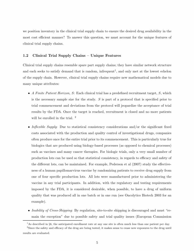
In this section, we consider a clinical trial supply chain of a general distribution topology, depicted

in Figure 1, where a central warehouse (CW), indexed as 0, supplies multiple country depots,

indexed by i = 1, 2, ..., I, and some sites directly, which are indexed by 0j where j = 1, 2, ..., J0 .

The other sites are satisfied via a particular depot i and are indexed ij where j = 1, 2, ..., Ji . For

convenience, we call the subsystem of country depot i and its corresponding sites ij the depot i

subsystem.

3.1 Assumptions and Notation

Throughout this paper, we make the following assumptions.

Assumption 1 (a) The clinical study has a finite patient horizon, S. (b) Each patient requires

one package or vial which is produced prior to the commencement of the trial. (c) Inventory (i.e.,

10

Figure 1: A general clinical trial supply chain.

dosages of drug in either package or vial form) cannot be transferred among sites or among country

depots. (d) Patient recruitment occurs only at trial sites and follows an independent Poisson process.

(e) Patients recruited at one site are unable to seek treatment from other sites. (f) In the event of

a temporary site-level stockout (with replenishment in-transit), patients will still enroll in the trial

and wait for resupply. (g) The patient fill rate is 100%, i.e., the system guarantees supply for the

first S patients whichever site they arrive to. (h) The transit times (i.e for shipping and regulatory

clearance) between CW and depots, CW and direct sites, and depots and sites are constant. (i) The

shipping costs from depots (or the CW) to testing sites (or direct sites) are negligible.

The first four assumptions are justified in §1.1-1.2. The assumption of a Poisson recruitment

process (1d) is widely used in the industry literature, see Abdelkafi et al. (2009) and references

therein. Clinical sites (e.g., hospitals, doctor’s offices) are chosen based on their ability to enroll

patients who meet the eligibility requirements of the trial. The recruitment rates can be estimated

based on the track record of patients visiting each site previously and/or data of previous trials for

the same disease. Assumption (1e) is a reflection of the geographical dispersement of clinical trials.

In reality, Assumption (1f) may or may not hold depending on the type of disease, the urgency

of treatment, and the location of trial sites. In this paper, we consider the case where patients

can and will wait for resupply if the site runs into a temporary drug shortage. Assumption (1g)

11

is justified in §1.2. The assumption of constant lead times (1h) is for simplicity and practitioners

have indicated that transit times may not be a significant source of variability.Assumption (1i) is

based on the fact that the costs associated with shipping from depots (or CW) to sites (or direct

sites) are often negligible as compared to those from CW to depots due to custom clearance and a

much larger geographic distance of the latter.

Consistent to the motivating example (§1.1), we assume that the clinical trial supply chain

works as follows: production of trial drug is done before the trial starts; inventory can be carried

by the testing sites, the depots and the CW; and lastly, sites are supplied by depots which are

supplied by the CW until the CW runs out of stock. In addition,

Assumption 2 (a) Inventory at each site is controlled by a continuous-review base-stock policy.

(b) Inventory at each country depot is controlled by a continuous-review batch ordering policy.

The assumption of a continuous-review inventory policy (2a and 2b) at sites and depots closely

represents modernized clinical trial supply chains. Through the use of integrated voice response

systems (IVRS), all doctors administering clinical trial drugs to patients are required to call in to

a system for instructions on which drug package is to be administered to the patient. Through this

system, both real-time inventory information is maintained and automated shipments to replenish

site-level inventory can be triggered (Byrom 2002). While sometimes it will take multiple demands

at a site to trigger an order, we make a simplifying assumption (2a), that is appropriate in high

value biologic trials, where an order is triggered each time a demand occurs.

We define the following notation:

System Parameters:

• λij , λ0j : Patient recruitment rates at sites ij and 0j respectively; λi =∑Ji

j=1 λij.

• Li, Lij , L0j : Lead times from CW to depot i, from depot i to site ij, and from CW to direct

site 0j, respectively.

• Di(L),Dij(L),D0j(L): Demand during lead time L at depot i, sites ij, and sites 0j respec-

tively.

Decision Variables:

• sij, s0j : Base-stock levels at sites ij and 0j respectively.

• ri, Qi: The reorder point and order quantity at depot i.

12

• s0: The initial stock at the CW, note that the CW cannot be replenished.

• xi: The expected number of shipments to depot i for the entire trial (excluding the initial

shipment).

• yi: The expected number of drug packages shipped to depot i for the entire trial (excluding

the initial shipment).

Costs and Service Levels:

• c: The cost of a drug package.

• Ki: The fixed cost of a shipment from the CW to depot i.

• vi: The variable shipping cost from the CW to depot i.

• ζ: The target patient fill rate for the trial.

• ζ ′: The target immediate fill rate at each site.

Our objective is to minimize system-wide inventory overage and shipping costs subject to a

100% patient fill rate (ζ = 100%, by Assumption 1g) and a high immediate fill rate (ζ ′), by setting

inventory levels (s0, ri, sij, s0j) and shipping quantities (Qi) appropriately.

3.2 The Role of The Finite Patient Horizon

The finite patient horizon, S, plays an important role in the patient fill rate requirement, ζ =

100%, which guarantees a sufficient supply for the first S patients arrived in the trial. Under this

requirement, s0 can be determined by S and other decision variables ri, Qi, sij and s0j for all j.

We make the following assumptions.

Assumption 3 (i) Each site starts with an initial inventory level equal to its base-stock level, depot

i starts with an initial inventory level ri +Qi, for all i. (ii) If the CW has insufficient stock to meet

the order quantity of a depot, then the depot takes whatever the CW has to offer.

Part (i) of Assumption 3 models real-world practice that it is more economical to fully stock

the depots and sites initially to achieve the scale economies in shipping. Part (ii) of Assumption

3 can be justified by observing that if otherwise, the CW may have to carry more inventory than

required just to meet a depot’s order quantity.

13

To ensure ζ = 100% while minimizing the inventory at the central warehouse, we must set

s0 = S − min{mini{ri + Qi + min

jsij},min

js0j}. (1)

To see this, we first observe that at the time when the CW runs out of stock, the system can still

satisfy min{mini{ri + qi + minj sij},minj s0j} many future patients without rejecting anyone due

to insufficient stock of the system. This can be easily seen by considering the worst-case scenario of

demand only arriving through one site. This observation implies that to guarantee ζ = 100% for the

entire trial, we should have at least S−min{mini{ri+qi+minj sij},minj s0j} many patients already

recruited by the time the CW runs out of stock. We also note that each order of size Qi placed by

depot i implies Qi patients already being recruited by this depot subsystem (by Assumption 3).

Thus, the total orders filled by the CW at any time must not exceed the total number of patients

recruited thus far. Excluding the Qi − qi patients from S because they are satisfied by depot i

at the time CW stocks out, we arrive at Eq. (1). Lastly, s0 ≥ 0 because setting minj s0j > S or

ri + Qi + minj sij > S for all i is clearly suboptimal.

By the finite patient horizon, it is also logical to assume the following stopping rules: (i) Site

0j (or ij) stops ordering when the total number of patients left to be recruited is no more than

its base-stock level s0j (or sij). (ii) Depot i stops ordering when the number of patients left to be

recruited is no more than ri + minj sij. By Eq. (1), the CW will never stockout before a direct site

or a depot stops ordering because when the CW runs out stock, Eq. (1) ensures that each direct

site/depot subsystem alone has enough stock to cover all the patients left to be recruited.

3.3 Shipping Costs and Model Formulation

We now calculate xi, yi and the expected shipping cost to depot i. By the stopping rule of §3.2,we only need to consider the first S − (ri + minj sij) patients recruited. The proof of the following

lemma is given in the Appendix.

Lemma 4 Suppose that among the first S − (ri + minj sij) patients recruited, Ni patients are

recruited by the depot i subsystem, then the number of orders placed by depot i after the trial starts,

Xi, satisfies the following inequalities:

�Ni

Qi� ≥ Xi ≥ �Ni

Qi� − 1, (2)

and the absolute difference between these bounds and Xi is at most 1.

14

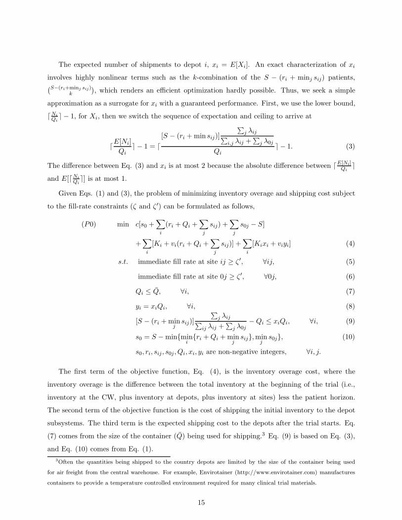
The expected number of shipments to depot i, xi = E[Xi]. An exact characterization of xi

involves highly nonlinear terms such as the k-combination of the S − (ri + minj sij) patients,(S−(ri+minj sij)

k

), which renders an efficient optimization hardly possible. Thus, we seek a simple

approximation as a surrogate for xi with a guaranteed performance. First, we use the lower bound,

�NiQi

� − 1, for Xi, then we switch the sequence of expectation and ceiling to arrive at

�E[Ni]Qi

� − 1 = �[S − (ri + min sij)]

∑j λij∑

i,j λij +∑

j λ0j

Qi� − 1. (3)

The difference between Eq. (3) and xi is at most 2 because the absolute difference between �E[Ni]Qi

�and E[�Ni

Qi�] is at most 1.

Given Eqs. (1) and (3), the problem of minimizing inventory overage and shipping cost subject

to the fill-rate constraints (ζ and ζ ′) can be formulated as follows,

(P0) min c[s0 +∑

i

(ri + Qi +∑

j

sij) +∑

j

s0j − S]

+∑

i

[Ki + vi(ri + Qi +∑

j

sij)] +∑

i

[Kixi + viyi] (4)

s.t. immediate fill rate at site ij ≥ ζ ′, ∀ij, (5)

immediate fill rate at site 0j ≥ ζ ′, ∀0j, (6)

Qi ≤ Q, ∀i, (7)

yi = xiQi, ∀i, (8)

[S − (ri + minj

sij)]∑

j λij∑ij λij +

∑j λ0j

− Qi ≤ xiQi, ∀i, (9)

s0 = S − min{mini{ri + Qi + min

jsij},min

js0j}, (10)

s0, ri, sij , s0j, Qi, xi, yi are non-negative integers, ∀i, j.

The first term of the objective function, Eq. (4), is the inventory overage cost, where the

inventory overage is the difference between the total inventory at the beginning of the trial (i.e.,

inventory at the CW, plus inventory at depots, plus inventory at sites) less the patient horizon.

The second term of the objective function is the cost of shipping the initial inventory to the depot

subsystems. The third term is the expected shipping cost to the depots after the trial starts. Eq.

(7) comes from the size of the container (Q) being used for shipping.3 Eq. (9) is based on Eq. (3),

and Eq. (10) comes from Eq. (1).3Often the quantities being shipped to the country depots are limited by the size of the container being used

for air freight from the central warehouse. For example, Envirotainer (http://www.envirotainer.com) manufactures

containers to provide a temperature controlled environment required for many clinical trial materials.

15

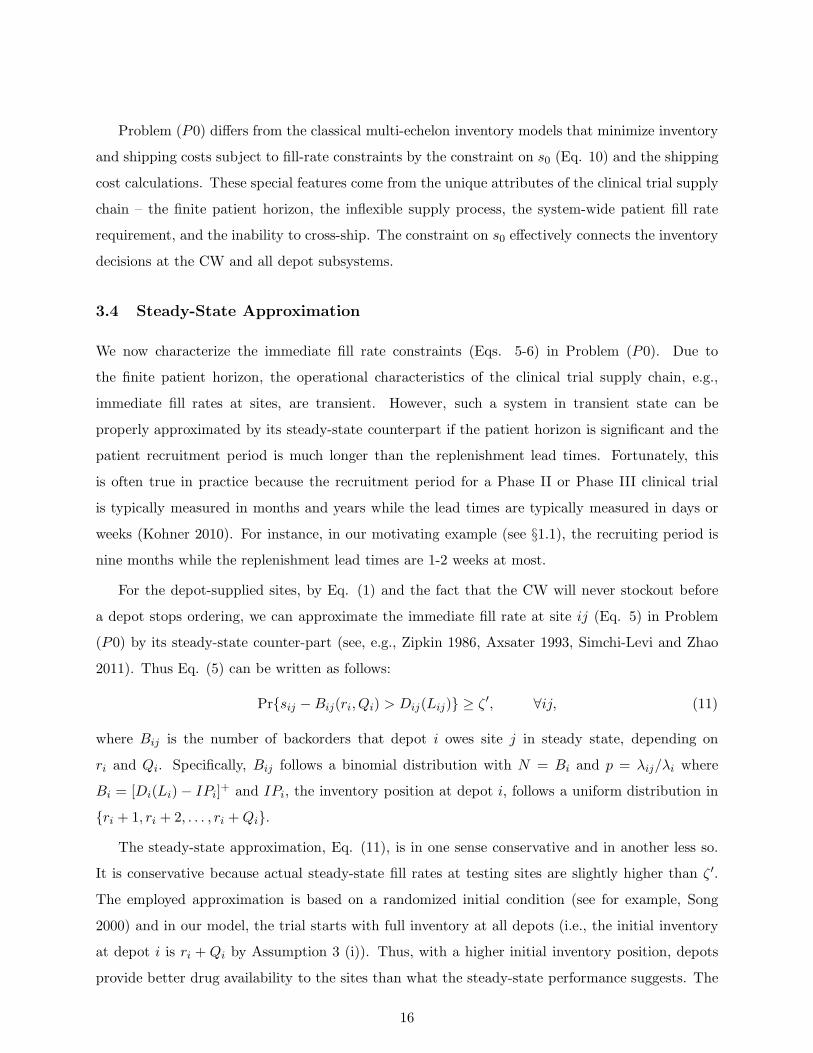
Problem (P0) differs from the classical multi-echelon inventory models that minimize inventory

and shipping costs subject to fill-rate constraints by the constraint on s0 (Eq. 10) and the shipping

cost calculations. These special features come from the unique attributes of the clinical trial supply

chain – the finite patient horizon, the inflexible supply process, the system-wide patient fill rate

requirement, and the inability to cross-ship. The constraint on s0 effectively connects the inventory

decisions at the CW and all depot subsystems.

3.4 Steady-State Approximation

We now characterize the immediate fill rate constraints (Eqs. 5-6) in Problem (P0). Due to

the finite patient horizon, the operational characteristics of the clinical trial supply chain, e.g.,

immediate fill rates at sites, are transient. However, such a system in transient state can be

properly approximated by its steady-state counterpart if the patient horizon is significant and the

patient recruitment period is much longer than the replenishment lead times. Fortunately, this

is often true in practice because the recruitment period for a Phase II or Phase III clinical trial

is typically measured in months and years while the lead times are typically measured in days or

weeks (Kohner 2010). For instance, in our motivating example (see §1.1), the recruiting period is

nine months while the replenishment lead times are 1-2 weeks at most.

For the depot-supplied sites, by Eq. (1) and the fact that the CW will never stockout before

a depot stops ordering, we can approximate the immediate fill rate at site ij (Eq. 5) in Problem

(P0) by its steady-state counter-part (see, e.g., Zipkin 1986, Axsater 1993, Simchi-Levi and Zhao

2011). Thus Eq. (5) can be written as follows:

Pr{sij − Bij(ri, Qi) > Dij(Lij)} ≥ ζ ′, ∀ij, (11)

where Bij is the number of backorders that depot i owes site j in steady state, depending on

ri and Qi. Specifically, Bij follows a binomial distribution with N = Bi and p = λij/λi where

Bi = [Di(Li) − IPi]+ and IPi, the inventory position at depot i, follows a uniform distribution in

{ri + 1, ri + 2, . . . , ri + Qi}.The steady-state approximation, Eq. (11), is in one sense conservative and in another less so.

It is conservative because actual steady-state fill rates at testing sites are slightly higher than ζ ′.

The employed approximation is based on a randomized initial condition (see for example, Song

2000) and in our model, the trial starts with full inventory at all depots (i.e., the initial inventory

at depot i is ri + Qi by Assumption 3 (i)). Thus, with a higher initial inventory position, depots

provide better drug availability to the sites than what the steady-state performance suggests. The

16

approximation is less conservative because Assumption 3 (ii) may also impact the actual fill rate

during the transient period near the end of the trial, but this would only apply to the last few

patients arriving at most to one depot subsystem (i.e. the subsystem encountering this assumption’s

exception). Hence, the negative impact of using a steady-state approximation on actual fill rates

is limited.

For sites supplied directly, we can use a similar logic to approximate the immediate fill rate

constraint at direct site 0j (Eq. 6) by its steady-state counter-part (see, e.g., Simchi-Levi and Zhao

2011):

Pr{s0j > D0j(L0j)} ≥ ζ ′, ∀0j. (12)

Problem (P0) is a nonlinear integer program with chance constraints as specified by Eqs. (11)-

(12). The trade-off is intuitively clear: the high immediate fill rates and high fixed shipping costs

mandate inventory being spread out to testing sites. On the other hand, the high drug cost and

high variable shipping costs favor centralizing inventory at the CW and/or depots. Problem (P0)

provides a mathematical framework to achieve the optimal balance.

3.5 Preliminary Results

The following lemma explores the dependence among the stock decisions at different locations.

Lemma 5 In the optimal solution to Problem (P0), sij is the minimum value to ensure the im-

mediate fill rate constraint at site ij given (ri, Qi) and unlimited supply from the CW; s0j is the

minimum value to ensure the immediate fill rate constraint at site 0j given unlimited supply from

the CW.

Proof. We first note that the CW never stocks out before depot i stops ordering by Assumption

(1g). Thus, we can treat the CW as if it has unlimited supply. Suppose the claim on sij is not

true, then there must exist an optimal solution to Problem (P0) such that the new solution of

reducing sij by one and increasing ri by one while keeping everything else unchanged still remains

feasible for all fill rate constraints. In this new solution, the xi, yi and s0 can only decrease while

everything else remains the same. Thus, the objective function can only decrease. We now have a

better solution which creates a contradiction to the optimality claim of the original solution. The

proof is completed for sij.

For s0j , we note that by the constraint of s0, the CW will never stockout before a direct site

stops ordering. By the same logic as that of sij, we can prove the desired result for s0j . �

17

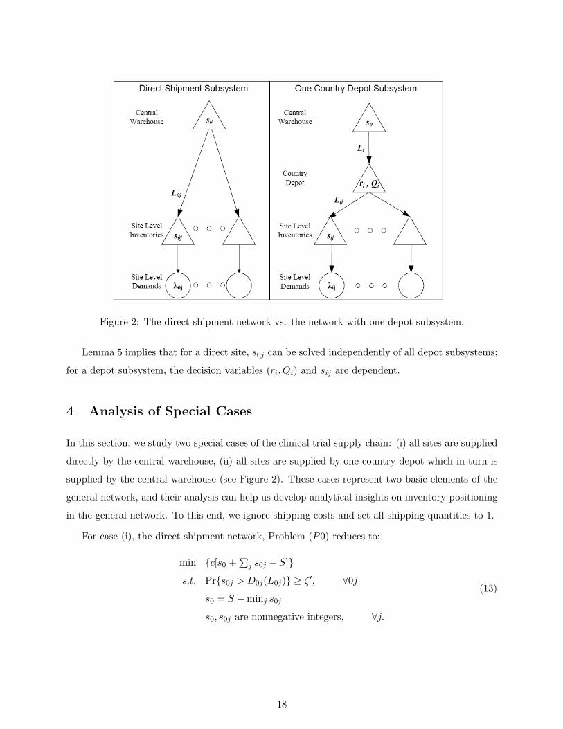
Figure 2: The direct shipment network vs. the network with one depot subsystem.

Lemma 5 implies that for a direct site, s0j can be solved independently of all depot subsystems;

for a depot subsystem, the decision variables (ri, Qi) and sij are dependent.

4 Analysis of Special Cases

In this section, we study two special cases of the clinical trial supply chain: (i) all sites are supplied

directly by the central warehouse, (ii) all sites are supplied by one country depot which in turn is

supplied by the central warehouse (see Figure 2). These cases represent two basic elements of the

general network, and their analysis can help us develop analytical insights on inventory positioning

in the general network. To this end, we ignore shipping costs and set all shipping quantities to 1.

For case (i), the direct shipment network, Problem (P0) reduces to:

min {c[s0 +∑

j s0j − S]}s.t. Pr{s0j > D0j(L0j)} ≥ ζ ′, ∀0j

s0 = S − minj s0j

s0, s0j are nonnegative integers, ∀j.

(13)

18

Replacing s0 in the objective function by its constraint yields,

min {c[∑j s0j − minj s0j ]}s.t. Pr{s0j > D0j(L0j)} ≥ ζ ′, ∀0j

s0, s0j are nonnegative integers, ∀j.

(14)

By Lemma 5, an optimal solution is to choose the smallest s0j that achieves the desired fill rate

at site 0j for all 0j given unlimited supply from the CW. This means that we should minimize

inventory at sites subject to the fill rate constraints.

For case (ii), the one country depot (i) system, Problem (P0) reduces to:

min {c[s0 + ri + 1 +∑

j sij − S]}s.t. Pr{sij − Bij(ri, 1) > Dij(Lij)} ≥ ζ ′, ∀j

s0 = S − ri − 1 − minj sij

s0, ri, sij are nonnegative integers, ∀j.

(15)

To simplify further, we place the constraint, s0 = S − ri − 1−minj sij, into the objective function,

then we have an equivalent problem:

min {c[∑j sij − minj sij]}s.t. Pr{sij − Bij(ri, 1) > Dij(Lij)} ≥ ζ ′, ∀j,

ri + 1 + minj sij ≤ S

ri, sij are nonnegative integers, ∀j.

(16)

Proposition 6 identifies the optimal solution to Problem (16), see the Appendix for a proof.

Proposition 6 The optimal solution to the following problem,

min {c[∑j sij]}s.t. Pr{sij − Bij(ri, 1) > Dij(Lij)} ≥ ζ ′, ∀j,

ri + 1 + minj sij ≤ S

ri, sij are nonnegative integers, ∀j,

(17)

is also optimal for Problem (16).

Proposition 6 reveals the optimal inventory positioning: To minimize the system-wide inventory,

one must minimize site level inventory. This can be done by stocking as much inventory at the

depot i as possible to reduce the needed stock at sites. Effectively, one can increase ri (to achieve

a lower sij) as long as s0 stays non-negative.

19

Both special cases indicate that we should pull inventory from sites back to the depot and/or

CW as much as possible subject to the immediate fill rate constraints at the sites. Such a strategy

differs from the multi-echelon inventory literature (see, e.g., Graves 1996) and the tradition in

clinical trials (Peterson, et al. 2004) which suggest to hold most of the safety-stock at the sites.

The special cases allow us to gain insights into general networks with multiple depot subsystems.

Consider a general network and suppose that in the optimal solution, depot i subsystem achieves

min{mini{ri + 1 + minj sij},minj s0j} in Eq. (10). Then, the optimal stocking strategy is to

minimize the total inventory at all depot subsystems except for depot i where one must minimize

the site level inventory. However, we do not know in advance which depot achieves the minimum

in Eq. (10) before we solve the Problem (P0). Thus, it is not trivial to make the optimal inventory

decisions for a general clinical trial supply chain, and it is even harder if we must also consider

shipping costs and shipping quantities.

5 Solution Methods

Problem (P0) is an integer quadratic program with probabilistic constraints. By the “coupling”

constraint on s0 (Eq. 10), we have to optimize jointly all depot subsystems in the network. This

constraint, combining with the quadratic constraints (Eqs. 8-9) and the integer requirement of the

decision variables, makes Problem (P0) very challenging to solve.

To develop an efficient method to solve Problem (P0), we first apply appropriate linearization

techniques to the quadratic terms and the “coupling” constraint to obtain a linear integer stochastic

programming (LISP) formulation (§5.1). As noted in the literature, LSIP is also very difficult to

solve (Dentcheva, Prekopa and Ruszczynski 2000), and one standard approach is to convert the

LISP into a deterministic equivalent formulation by the well-known concept of p-efficient points

(Prekopa 2003). However, the set of p-efficient points can be extremely large, and this concept is

associated with a specific probability distribution and thus not applicable here. Yet, by leveraging a

unique feature of Problem (P0), the “finite patient horizon”, and Lemma 5, we can derive a “finite”

set of deterministic linear constraints equivalent to the fill rate constraints (§5.2). Consequently,

we reformulate the original problem into an equivalent linear integer program (§5.3).

20

5.1 Linearization

Linearization of the coupling constraint on s0 is done by changing the equality sign to an inequality

sign, as follows,

s0 ≥ S − min{mini{ri + Qi + min

jsij},min

js0j}.

The optimal solution shall remain the same regardless of this change because the objective is to

minimize the total supply chain cost of the trial. Hence, in the optimal solution, s0 will be driven

down to S − min{mini{ri + Qi + minj sij},minj s0j} to achieve the lowest cost possible.

We linearize the quadratic terms xiQi by the binary representation of Qi = 20yi0 +21yi1 + . . .+

2nyin, where n = �log(Q)� and yi0, . . . , yin are binary variables (Billionnet, et. al 2008). Then,

xiQi = 20xiyi0 + 21xiyi1 + . . . + 2nxiyin. Let Yik = xiyik where k = 0, 1, . . . , n, then we have

yi = xiQi = 20Yi0 + 21Yi1 + . . . + 2nYin. (18)

Since Yik is a product of a binary variable yik and a bounded variable 0 ≤ xi ≤ S, it satisfies the

following set of inequalities,

Yik ≤ Syik

Yik ≤ xi

Yik ≥ xi − S(1 − yik).

Finally, the constraint yi = xiQi is equivalent to the following constraints,

yi = 20Yi0 + 21Yi1 + . . . + 2nYin

Yik ≤ Syik, k = 0, 1, . . . , n

Yik ≤ xi, k = 0, 1, . . . , n

Yik ≥ xi − S(1 − yik), k = 0, 1, . . . , n.

5.2 Chance Constraints

The fill-rate constraints for the depot i subsystem are

Pr{sij − Bij(ri, Qi) > Dij(Lij)} ≥ ζ ′, ∀ij.

To convert these chance constraints into a set of deterministic linear constraints, we define si =

(ri, Qi, si1, si2, ..., siJi) to be an inventory position for the depot i subsystem.

Definition 7 We call si = (ri, Qi, si1, si2, ..., siJi) a “minimum inventory position” for the depot i

subsystem if it is feasible, i.e., it satisfies all the immediate fill rate constraints for depot i subsystem,

and there does not exist a feasible inventory position that is smaller than si component-wisely.

21

For each depot subsystem, the number of the minimum inventory positions is bounded from

above by S × Q (by Lemma 5). We define the set of minimum inventory positions for depot i

subsystem to be Ii = {s(1)i , s

(2)i , . . . , s

(ni)i } where ni is the size of Ii. We can rewrite the fill-rate

constraints (Eq. 5) for depot i subsystem as follows,

si ≥ μi1s(1)i + μi2s

(2)i + . . . + μini s

(ni)i , (19)

where μi1, . . . , μini are binary variables, μi1 + . . . + μini = 1, and ≥ is component-wise. This takes

us to the following algorithm for identifying the set of minimum inventory positions for the depot

i subsystem.

Step 0. Set Ii = ∅, ri = 1, Qi = 1.

Step 1. For each pair of ri and Qi where ri ≤ S and Qi ≤ Q, find the smallest sij at sites that

satisfy the immediate fill-rate constraints. Let the output be si = (ri, Qi, si1, . . . , siJi). If there

does not exist an element in Ii that is smaller than or equal to this output component-wisely,

then the output is a minimum inventory position and Ii = Ii ∪ {si}.

Step 2. Output the set of all minimum inventory positionings Ii.

In Step 1, we utilize the two-moment approximation (see, e.g., Graves 1985) to calculate the fill

rates, which is proven to be fast and sufficiently accurate. The computational complexity for

generating Ii is at most O(S2 × Q2 × Ji). In fact, we can generate Ii much faster because given a

Qi, when ri increases beyond a certain level, the smallest sij at sites shall remain constant.

5.3 Integer Programming Reformulation

We are now ready to present an equivalent linear integer programming reformulation of Problem

(P0). Note that s0j can be optimized separately (Lemma 5), we let s∗0j be the optimal solution.

(P1) min c[s0 +∑

i

(ri + Qi +∑

j

sij) +∑

j

s∗0j − S]

+∑

i

[Ki + vi(ri + Qi +∑

j

sij)] +∑

i

[Kixi + viyi]

s.t. si ≥ μi1s(1)i + . . . + μini s

(ni)i , ∀i,

μi1 + . . . + μini = 1, ∀i,

yi = 20Yi0 + 21Yi1 + . . . 2nYin, ∀i,

Yik ≤ Syik, k = 1, . . . , n,∀i,

22

Yik ≤ xi, k = 1, . . . , n,∀i,

Yik ≥ xi − S(1 − yik), k = 1, . . . , n,∀i,

[S − (ri + minj

sij)]∑

j λij∑ij λij +

∑j λ0j

− Qi ≤ yi, ∀i,

s0 + {ri + Qi + sij} ≥ S, ∀i, j,

s0 + minj

s∗0j ≥ S,

s0, ri, sij, Qi, xi, yi, Yik are non-negative integers, μij , yik binary, ∀i, j, k.

Problem (P1) is a linear integer program which can solved by standard integer programming solvers.

6 Numerical Study

In this section, we conduct a numerical study on a hypothetical real-life example. The objective is

two-fold: (i) to test the efficiency of the solution method and (ii) to develop insights on inventory

positioning in clinical trial supply chains. We also demonstrate the potential impact of the site

network on the supply chain costs and study the trade-off between inventory overage and recruit-

ment time. The practical intent of the model is to provide decision support to clinical trial supply

managers and to facilitate their communication with the study managers regarding the enrollment

plans and countries/sites to be include in a trial.

6.1 Example Details and Computational Performance

We report the computational performance of the solution method (see §5) on the example in §1.1.This example is motivated by data 4 from a real-life Phase III clinical trial that enrolled patients

over a 9-month period. Data relevant to this trial’s inventory decisions is summarized in Table 2.

By Table 2, the total enrollment rate is 2.18 patients per day. Because the patient horizon,

S, is 600 patients, the expected recruitment period is 600 patients/2.18 patients per day ≈ 275

days, which is significantly longer than the importation lead times, and thus the operational char-

acteristics of the system in transient states can be reasonably approximated by their steady-state

counterparts. For this numerical study, we assume that all countries use country depots and the

intra-country lead time from a depot to a site is one day. Since manufacturing was done outside of

all site countries, all distribution goes through their respective country’s customs and importation

processes. Shipping cost estimates to the country depots are summarized in Table 3.

4Please note that the data is disguised as requested by the study sponsor.

23

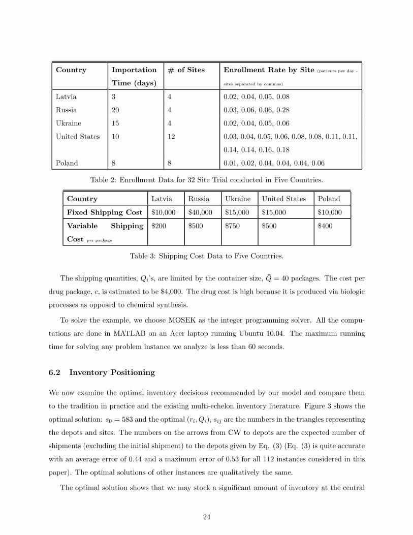
Country Importation

Time (days)

# of Sites Enrollment Rate by Site (patients per day -

sites separated by commas)

Latvia 3 4 0.02, 0.04, 0.05, 0.08

Russia 20 4 0.03, 0.06, 0.06, 0.28

Ukraine 15 4 0.02, 0.04, 0.05, 0.06

United States 10 12 0.03, 0.04, 0.05, 0.06, 0.08, 0.08, 0.11, 0.11,

0.14, 0.14, 0.16, 0.18

Poland 8 8 0.01, 0.02, 0.04, 0.04, 0.04, 0.06

Table 2: Enrollment Data for 32 Site Trial conducted in Five Countries.

Country Latvia Russia Ukraine United States Poland

Fixed Shipping Cost $10,000 $40,000 $15,000 $15,000 $10,000

Variable Shipping

Cost per package

$200 $500 $750 $500 $400

Table 3: Shipping Cost Data to Five Countries.

The shipping quantities, Qi’s, are limited by the container size, Q = 40 packages. The cost per

drug package, c, is estimated to be $4,000. The drug cost is high because it is produced via biologic

processes as opposed to chemical synthesis.

To solve the example, we choose MOSEK as the integer programming solver. All the compu-

tations are done in MATLAB on an Acer laptop running Ubuntu 10.04. The maximum running

time for solving any problem instance we analyze is less than 60 seconds.

6.2 Inventory Positioning

We now examine the optimal inventory decisions recommended by our model and compare them

to the tradition in practice and the existing multi-echelon inventory literature. Figure 3 shows the

optimal solution: s0 = 583 and the optimal (ri, Qi), sij are the numbers in the triangles representing

the depots and sites. The numbers on the arrows from CW to depots are the expected number of

shipments (excluding the initial shipment) to the depots given by Eq. (3) (Eq. (3) is quite accurate

with an average error of 0.44 and a maximum error of 0.53 for all 112 instances considered in this

paper). The optimal solutions of other instances are qualitatively the same.

The optimal solution shows that we may stock a significant amount of inventory at the central

24

Figure 3: The optimal inventory decisions for c = $4, 000.

warehouse, and a sizable amount of inventory at country depots relative to the corresponding

site level inventory. By doing so, we can achieve significant savings in inventory overage (from

the current 100%-200% to 186 packages ∼ 31% of the patient horizon) while maintaining a high

immediate fill rate at all sites and providing a guaranteed supply for the first S (600) patients. The

resulting minimum inventory overage and shipping cost is $1.45 million.

This solution differs qualitatively from the tradition in practice, see §1.1 and Peterson, et al.

(2004), which aims to save shipping cost by holding most inventory at sites and depots but is

suboptimal due to its significant inventory overage. This solution is also qualitatively different

from the multi-echelon inventory literature which suggests to hold most of the safety-stock at the

lowest echelon. This new insight on inventory positioning comes from the unique features of the

clinical trial supply chains (see §1.2).To study the impact of drug cost, we solve the example again but for c = $2, 000, $6, 000, $8, 000,

$10, 000. The result is summarized in Figure 4. We observe that as c increases, the reorder points

and shipping quantities at country depots tend to decrease which results in a lower inventory

overage but a higher shipping cost. The total cost increases significantly as the drug cost increases.

6.3 Impact of Site Network

To study how the network of clinical sites affects the inventory overage and total cost, we compare

the depth and the breadth strategies where the former has only a few countries but each country

25

Figure 4: The impact of drug cost.

has many sites, the latter does the opposite – has many countries but each country has fewer sites.

Specifically, we consider the following two instances of the example with c = $4, 000:

• Depth: the network includes Russia (4 sites), the U.S. (11 sites) and Poland (6 sites).

• Breadth: the network includes Latvia (4 sites), Russia (4 sites), Ukraine (4 sites), the U.S.

(6 sites) and Poland (4 sites).

To make these instances comparable, we select sites so that the expected recruitment time is 350

days for both instances.

Figure 5 shows the inventory overage, shipping and total cost of the two instances. As we can

see, the depth strategy has a lower inventory overage cost and a lower shipping cost as compared

to the breadth strategy. To explain why the depth strategy outperforms the breadth strategy in

inventory overage, we pick the U.S. and calculate the inventory per site in each strategy. As we

move from the depth strategy to the Breadth strategy, the number of sites in the U.S. decreases

from 11 to 6. Dividing the total inventory (ri +∑

j sij) at the depot subsystem of the U.S. by

the number of the sites, we find that the inventory per site of the depth (breadth) strategy is 2.91

(3.16, respectively). So the insight is clear: the more sites that a depot serves, the less inventory

per site is required, which is the well known risk pooling effect.

26

Figure 5: The impact of site network: depth vs. breadth strategies.

6.4 Overage vs. Recruitment Time

One important issue that clinical trial management must address is how many countries to include

in the trial. Intuitively, the more countries to include in the trial, the shorter the recruitment time

but the higher the inventory overage. To study the trade-off between the inventory overage and

the expected enrollment time, we take the enrollment data of the motivating example and examine

what would happen to the inventory overage, total cost and the expected enrollment time as we

add countries into the trial in the order of descending enrollment rates.

The result is summarized in Figure 6 where “2-country” refers to a trial with only the U.S. and

Russia, “3-country” refers a trial with the U.S., Russia and Poland, and so on. This figure shows

that increasing the number of countries results in sizable decreases in the expected recruitment

time but significant increases in the inventory overage. Given roughly the same shipping cost for

all cases, the total supply chain cost increases significantly from around $0.987 million to about

$1.45 million while the expected recruitment time decreases from 373 days to 275 days.

For a clinical supply manager, with a limited budget to spend on clinical supplies and a mandate

to not delay the trial, being able to show the tradeoff between overages (total supply chain costs)

and recruiting time is critical to their discussion with the rest of the clinical trial team. Some

countries may be left out of the trial because marginal decreases in recruiting time do not justify

the additional costs in supplies.

27

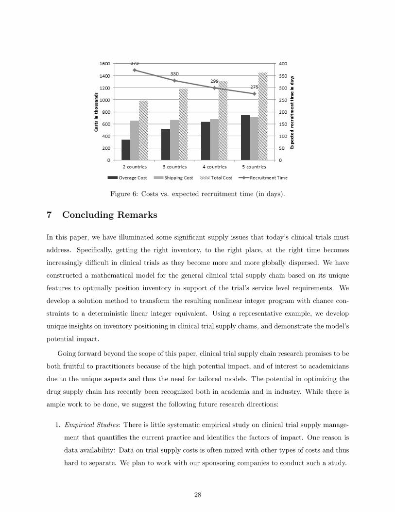
Figure 6: Costs vs. expected recruitment time (in days).

7 Concluding Remarks

In this paper, we have illuminated some significant supply issues that today’s clinical trials must

address. Specifically, getting the right inventory, to the right place, at the right time becomes

increasingly difficult in clinical trials as they become more and more globally dispersed. We have

constructed a mathematical model for the general clinical trial supply chain based on its unique

features to optimally position inventory in support of the trial’s service level requirements. We

develop a solution method to transform the resulting nonlinear integer program with chance con-

straints to a deterministic linear integer equivalent. Using a representative example, we develop

unique insights on inventory positioning in clinical trial supply chains, and demonstrate the model’s

potential impact.

Going forward beyond the scope of this paper, clinical trial supply chain research promises to be

both fruitful to practitioners because of the high potential impact, and of interest to academicians

due to the unique aspects and thus the need for tailored models. The potential in optimizing the

drug supply chain has recently been recognized both in academia and in industry. While there is

ample work to be done, we suggest the following future research directions:

1. Empirical Studies: There is little systematic empirical study on clinical trial supply manage-

ment that quantifies the current practice and identifies the factors of impact. One reason is

data availability: Data on trial supply costs is often mixed with other types of costs and thus

hard to separate. We plan to work with our sponsoring companies to conduct such a study.

28

2. Applications of Models: While the model presented in this paper illustrates enormous oppor-

tunities to provide value for clinical trial supply chains, applying this model in the real-world

practice would help refine and validate it.

3. Integrating Inventory and Project Decisions: It is of great interest to integrate the inventory

decisions (discussed in this paper) with clinical trial project decisions, such as country/site

selection, design of the study and protocols, and staffing plan to optimize not only the supply

chain costs but also the patient and medical expenses.

4. Relaxing the 100% patient fill rate: while it is ideal (and often the mandate) to guarantee

medical supply for the first S patients, it may be overly conservative in some cases. Relaxing

this constraint requires a significant modification of the mathematical model in calculating

the fill rates and shipping costs as one must consider the possibility of rejecting patients

during the trial.

Appendix

Proof of Lemma 4: Consider the first S − (ri + minj sij) patients recruited. Suppose Ni patients

are recruited by the depot i subsystem, then the number of orders placed by depot i after the trial

starts, Xi, is given as follows:

Xi = 0, if 0 ≤ Ni < Qi

Xi = 1, if Qi < Ni < 2Qi

...

Xi = n, if nQi < Ni < (n + 1)Qi.

If Ni = nQi for n ≥ 1, then we have two possibilities: Xi = n if the last patient of the first

S − (ri + minj sij) patients is recruited by depot i subsystem; Xi = n + 1 otherwise. This is true

because depot i orders only when both of the following two conditions are satisfied: (i) its local

inventory position drops to ri (ii) there are more than ri + minj sij patients left to be recruited.

When the Nith patient arrives at depot i subsystem, in the first possibility, condition (i) is satisfied

but condition (ii) is not; in the second possibility, both conditions are satisfied, and that is why

one more order is placed. The rest of the proof is straightforward. �

Proof of Proposition 6: Denote the solution of Problem (17) to be s′. Suppose that the propo-

29

sition is not true, then there must exist a solution to Problem (16), s′′, such that

∑

j

s′ij − minj

s′ij >∑

j

s′′ij − minj

s′′ij. (20)

By Lemma 5, we note that given ri, sij are uniquely determined by the fill rate constraints in

both Problem (16) and (17). In addition, sij is non-increasing in ri (this is clearly true as a higher

stocked the regional warehouse only reduces the need of inventory at sites). Thus, Inequality (20)

implies r′i < r′′i . To see this, we define j′ = argminj{s′ij}, j′′ = argminj{s′′ij}, and consider two

cases:

• Case 1: j′ = j′′. Then inequality (20) implies∑

j �=j′ s′ij >

∑j �=j′ s

′′ij . This is only true when

r′i < r′′i .

• Case 2: j′ = j′′. Rewrite Inequality (20) as

∑

j �=j′,j′′s′ij + s′ij′′ >

∑

j �=j′,j′′s′′ij + s′′ij′ .

Suppose r′i ≥ r′′i , then s′ij ≤ s′′ij for all j, and by the above inequality s′ij′′ > s′′ij′ . Together

with s′′ij′ ≥ s′′ij′′ (by definition of j′′), we must have s′ij′′ > s′′ij′′ which contradicts to the fact

that s′ij ≤ s′′ij for all j. Thus we must have r′i < r′′i .

r′i < r′′i implies s′ij ≥ s′′ij for all j. If there is one j such that s′ij > s′′ij, this creates a contra-

diction to the assumption that s′ is optimal for Problem (17). If s′ij = s′′ij for all j, this creates

a contradiction to Inequality (20). In conclusion, the optimal solution s′ for Problem (17) is also

optimal for (16). �

References

[1] Abdelkafi, C., H. L. B. Beck, B. David, C. Druck, M. Horoho (2009). Balancing risk and costs

to optimize the clinical supply chain – a step beyond simulation. Journal of Pharmaceutical

Innovations 4: 96-106.

[2] Andrews, C. (2004). Strategic Value of Clinical Supplies. Pharmaceutical Engineering 24(5).

[3] Axsater, S. (1990). Simple solution procedures for a class of two-echelon inventory problems.

Operations Research 38(1) 64–69.

30

[4] Axsater, S. (1993a). Continuous review policies for multi-level inventory systems with stochas-

tic demand. In S. Graves, A. Rinnooy Kan, P. Zipkin, (eds.). Logistics of Production and

Inventory. Elsevier (North-Holland), Amsterdam. The Netherlands.

[5] Barnett International (2010). Focus on Study Drug. Good Clinical Practice: A Question &

Answer Reference Guide 15(15) 2010.

[6] Billionnet, A. and Elloumi, S. and Lambert, A. (2008). Linear Reformulations of Integer

Quadratic Programs. Modelling, Computation and Optimization in Information Systems and

Management Sciences 14 43–51.

[7] Byrom, B. (2002). Using IVRS in clinical trial management. Applied Clinical Trials October.

[8] Caggiano, K. E., P. L. Jackson, J. A. Muckstadt, J. A. Rappold (2007). Optimizing Ser-

vice Parts Inventory in a Multiechelon, Multi-Item Supply Chain with Time-Based Customer

Service-Level Agreements. OPERATIONS RESEARCH 55(2) 303–318.

[9] Caglar, D., C. L. Li, D. Simchi-Levi (2004). Two-echelon spare parts inventory system subject

to a service constraint. IIE Transactions 36(7) 655 – 666.

[10] Dentcheva, D. and Prekopa, A. and Ruszczynski, A. (2000). Concavity and efficient points of

discrete distributions in probabilistic programming. Mathematical Programming 89 55–77.

[11] European Commission Enterprise Directorate-General (2000). Manufacture of Investigational

medicinal products. Good manufacturing Practices 4(13) July 2003.

[12] Fleischhack, A. (2009). An investigation of clinical trial supply chains. Ph.D Thesis, Depart-

ment of Supply Chain Management and Marketing Science. Rutgers University – New Newark

and New Brunswick. NJ.

[13] Getz, K. A., A. de Bruin (2000). Breaking the development speed barrier: Assessing successful

practices of the fastest drug development companies. Drug Information Journal 34 p725 –

736.

[14] Glickman, S. W., J. G. McHutchison, E. D. Peterson, C. B. Cairns, Robert A. Harrington,

Robert M. Califf, Kevin A. Schulman (2009). Ethical and scientific implications of the global-

ization of clinical research. N Engl J Med 360(8) 816–823.

[15] Graves, S. C. (1985). A multi-echelon inventory model for a repairable item with one-for-one

replenishment. Management Science 31(10) 1247–1256.

31

[16] Graves, S. C. (1996). A multiechelon inventory model with fixed replenishment intervals.

Management Science 42(1) 1–18.

[17] Klim, A. (2010). BRIC by BRIC: Laying a path to success. Pharmaceutical Manufacturing

and Packing Sourcer Summer 2010.

[18] Kohner, N. (2010). Temperature

Controlled Shipping in Clinical Trials: A Rising Requirement. Almac Group White Paper

available at http://www.arradx.com/papers/Papers/Temperature%20Controlled%20Shipping

%20in%20Clinical%20Trials.pdf and accessed on February 2, 2010.

[19] Le Chevalier, T., D. Brisgand, J.Y. Douillard, J.L. Pujol, V. Alberola, A. Monnier, A. Riviere,

P. Lianes, P. Chomy, S. Cigolari (1994). Randomized study of vinorelbine and cisplatin versus

vindesine and cisplatin versus vinorelbine alone in advanced non-small-cell lung cancer: results

of a European multicenter trial including 612 patients. J Clin Oncol 12(2) 360–367.

[20] Lis, F., P. Gourley, P. Wilson, M. Page (June 1, 2009). Global supply chain management.

Applied Clinical Trials Online.

[21] McDonnell, W., H. Mooraj (2009). Case Study: Visualizing Clinical Trial Demand. Industry

Value Chain Strategies AMR Research. April 2009.

[22] Muckstadt, J.A. (2005). Analysis and algorithms for service parts supply chains. Springer

Verlag.

[23] Oncolytics Biotech Inc. (2003). Oncolytics Biotech Inc. Announces Completion of Manufac-

turing Process Development for REOLYSIN(R). PR Newswire, February 6, 2003.

[24] Pederson, C., T. Petaja, G. Strauss, H.C. Rumke, A. Poder, J.H. Richardus, B. Spiessens,

D. Descamps, K. Hardt, M. Lehtinen, G. Dubin (2007). Immunization of Early Adolescent

Females with Human Papillomavirus Type 16 and 18 L1 Virus-Like Particle Vaccine Containing

AS04 Adjuvant. Journal of Adolescent Health 40(6) 564–571.

[25] Peterson, M., B. Byrom, N. Dowlman, D. McEntegart (2004). Optimizing clinical trial supply

requirements: simulation of computer-controlled supply chain management. Clinical Trials

1(4) 399–412.

[26] Powell, Mark (2010). Presentation by Senior Vice President, Pharmaceutical Development,

Bristol-Myers Squibb. Argyle Executive Forum’s 2010 Leadership in Pharmaceuticals &

32

Biotechnology conference. June 22, 2010. New York, New York. Transcript available at

http://www.argyleforum.com/Thought-Leadership accessed on July 8, 2011.

[27] Prekopa, A. (2003). Probabilistic programming. Handbooks in Operations Research and Man-

agement Science 10 267–351.

[28] Ravichandran, N. (1995) Stochastic analysis of a continuous review perishable inventory system

with positive lead time and Poisson demand European Journal of Operational Research 84(2)

444–457.

[29] Roberts, T., T.J. Lynch, B.A. Chabner (2004). The phase III trial in the era of targeted

therapy: unraveling the “go or no go” decision. Journal of Clinical Oncology 21(19) 3683–95.

[30] Rowland, C. (2004). Clinical trials seen shifting overseas. International Journal of Health

Services 34(3) p555 – 556.

[31] Shah, N. (2004). Pharmaceutical supply chains: key issues and strategies for optimisation.

Computers and Chemical Engineering 28(6-7) 929–941.

[32] Sherbrooke, C. C. (1968). Metric: A multi-echelon technique for recoverable item control.

Operations Research 16(1) 122–141.

[33] Simchi-Levi, D., Y. Zhao. (2005). Safety Stock Positioning in Supply Chains with Stochastic

Lead Times. Manufacturing & Service Operations Management 7(4) 295–318.

[34] Simchi-Levi, D., Y. Zhao (2011). Performance Evaluation of Stochastic Multi-Echelon Inven-

tory Systems: A Survey. Advances in Operations Research 1-34.

[35] Song, J. S. (2000). A note on Assemble-to-Order systems with batch ordering. Management

Sciences 46, 739-943.

[36] Svoronos, A., P. Zipkin (1991). Evaluation of one-for-one replenishment policies for multiech-

elon inventory systems. Management Science 37(1) 68–83.

[37] Thiers, F.A., A.J. Sinskey, E.R. Berndt (2008). Trends in the globalization of clinical trials.

Nature Reviews Drug Discovery 7 p13 – 15.

[38] Vallance, P. (2011).

Presentation at the Cowen and Company 31st Annual Health Care Conference in Boston.

33

Webcast available at http://www.gsk.com/investors/presentations webcasts.htm/ accessed on

March 17, 2011.

[39] Zipkin, P. (1986). Stochastic lead-times in continuous-time inventory models. Naval Research

Logistics Quarterly, 33, 763-774.

[40] Zipkin, P. (2000). Foundations of Inventory Management. McGraw Hill, Boston.

34