Filomat 26:3 (2012), 573–583DOI 10.2298/FIL1203573L

Published by Faculty of Sciences and Mathematics,University of Nis, SerbiaAvailable at: http://www.pmf.ni.ac.rs/filomat

Portfolio problems based on jump-diffusion models

Tiantian Liua, Jun Zhaob, Peibiao Zhaoc

aDept. of Applied Mathematics, Nanjing University of Science and Technology, Nanjing 210094, P. R. ChinabBaixia Subbranch, Guangfa Bank of China, Nanjing 210001, P. R. China

cDept. of Applied Mathematics, Nanjing University of Science and Technology, Nanjing 210094, P. R. China

Abstract. Zhou and Li [49] by virtue of stochastic linear-quadratic control theory studied the optimalportfolio problems with the asset price process satisfying a diffusion stochastic differential equation, andproposed the celebrated LQ framework and the efficient frontier for the given portfolio problem. In thispaper, we consider the optimal portfolio problems based on the asset price process satisfying a jump-diffusion stochastic differential equation. Similarly, we also arrive at the efficient frontier of the optimalportfolio selection problem. The conclusions obtained here can be regarded as a natural generalization ofthe work by Zhou and Li [49].

1. Introduction

Since Markowitz [25, 26], many researchers studied the portfolio theory, W. Sharpe [42], J. Lintner [23]and J. Mossin [32] respectively put forward the famous capital asset pricing model (CAPM); Fama [11]and Samuelson [39] proposed the efficient market theory; Merton [30] derived the capital gains rate is alognormal distribution of the capital asset pricing model in the case of continuous-time transactions; Ross[38] developed breakthroughly the capital asset pricing model, and put forward the arbitrage pricing theory(APT), it laid a solid foundations for the development of modern portfolio theory and the growth of financialmarkets, and so on. On the other hand, many scholars consider the applications with the improved mean-variance models such as CVaR, spectral risk measures, variance hedge, dynamic portfolio with transactioncosts, etc., and obtain some celebrated works, one can refer to [2, 6, 7, 9, 15, 18, 22, 24, 34, 41, 45, 46] for details.

After the pioneering work of Markowitz, the single-period mean-variance model was quickly extendedto the multi-period portfolio selection problems. However, comparing to the single-period model, theanalytical solution to multi-period models had not given until the work was posed by Merton [29]. Thestudy of multi-period portfolio problems has been dominated by the maximizing the expected utility ofthe final wealth, namely maximize E[U(x(T))], where U is a utility function. Logarithmic, exponential,quadratic utility functions have been extensively studied before. The shortcoming of these findings isthe lack of long-term consideration of the optimal investment strategy. On the one hand, it is difficultto determine the investor’s utility functions. On the other hand, the transaction information of risk andexpected return has not been clear, many investors depended on intuition to make decisions. In this sense,

2010 Mathematics Subject Classification. Primary 90A09; Secondary 91B32, 90C47Keywords. Jump-diffusion model, mean-variance, portfolio, stochastic linear-quadratic methodReceived: 04 March 2011; Accepted: 18 October 2011Communicated by Predrag StanimirovicResearch supported by a Grant-in-Aid for NJUST Research Funding, No.2010GJPY024 and No. 2011YBXM120 and by NNSF of

China (11071119)Email addresses: jsxzltt@126.com (Tiantian Liu), jongjong28@sina.com (Jun Zhao), pbzhao@mail.njust.edu.cn (Peibiao Zhao)

T.T. Liu et al. / Filomat 26:3 (2012), 573–583 574

Markowitz’s mean-variance approach has not been fully utilized in the dynamic, multi-period investmentdecisions.

The research initially on the portfolio, was only limited to single-period portfolio problems. In the actualinvestment environment, the distribution of asset returns often changes with different stages. The articleof Mossin [33] published in 1968 was the first to consider multi-stage portfolio problems, he extended thesingle-stage model of Markowitz to multi-stage situation with the dynamic programming methods. In1972, Merton [29] gave the standard form of the analytical solution of Markowitz mean-variance model.Since then, Merton [27, 28] and Samuleson [40] constructed a reference frame of multi-stage model. Chen,Jen and Zionts [4] improved Smith’s model and extended to the multi-stage situation. Hakansson [17]gave the analysis of multi-stage mean-variance. Mossin [32], Ross [38] studied the mean-variance hedgingproblem, the conclusion of [32] is obtained based on the following assumptions: all the factors (includinginterest rates, volatility, etc.) are identified, constant and does not changes over time. In [12], the authorsconsidered and obtained the solution to the variance minimization problem by embedding the constraintequations into the target functions. In 2000, Zhou and Li [49] used stochastic linear quadratic controltheory to study the problem of mean-variance optimization, and they obtained the best analytical solutionof the optimal investment strategy and the explicit representation of effective frontier of the mean-varianceportfolio selection problem. This article is unusual in that the original problem being changed into astochastic optimal linear quadratic problem, and solved it using linear quadratic theory. The solution ofthe original problem can be obtained by dealing with the transformed problem. Its contribution is to linkthe standard portfolio choice problem with stochastic control model, and to provide a general frameworkto deal with more complex situations.

It is generally believed that the stock price follows geometric Brownian motion, Zhou and Li’s researchis based on the process of financial asset prices being a continuous process with respect to time. However, infinancial practice, the process of financial asset prices is not necessarily a continuous process. For example,subjected to significant information (such as sudden major events, policy changes, etc.), a jump of upsand downs of the stock price will occur. The time and impact of such information occurring is random,therefore, one can describe it by the Poisson process. In this paper, similar to the work by Zhou and Li[49], we study the mean variance portfolio problem based on the asset prices satisfying the jump-diffusionstochastic differential equation, and also arrive at the efficient frontier.

The organization of this paper is as follows. The first two sections briefly introduce some necessarynotations and terminologies. Section 3 proposes a model based on a stochastic jump-diffusion differentialequation framework. The authors get an analytic solution of the optimal control problem by using thestochastic linear-quadratic method. Similarly, we also arrive at the efficient frontier. The results posed herecan be regarded as a natural generalization of Zhou and Li [49].

2. Preliminaries

2.1. Mean-variance models

The portfolio based on the mean-variance that was originally proposed by Markowitz is the core ofmodern portfolio theory. It uses probability theory and optimization techniques model to get the investmentbehavior under uncertainty. Investment income is described by the mean income, and investment risk isdescribed by income variance. Assume that the investor chooses n kinds of risk assets to do invest. Forconvenience, we denote by the following

R + (r1, r2, · · · , rn)T is the expected return vector of risky assets;∑+ (σi j)n×n is the risk covariance matrix of asset returns;

x = (x1, x2, · · · , xn)T is the vector with investment ratio xi in i-th risk asset;l = (1, 1, · · · , 1)T is the vector with all components being 1;We call r(x) = RTx, σ2(x) = xT∑ x as the portfolio expected return, the risk, respectively.Then, Markowitz’s mean-variance model can be expressed in two mathematical models: The first model

T.T. Liu et al. / Filomat 26:3 (2012), 573–583 575

is as follows

Min xT∑

x

s.t.

RTx = µlTx = 1Ax ≤ B

where µ is the level of expected return given by investor, Am×n is a constant matrix, B is an n-dimensionalconstant vector

The second model is as follows

Max RTx

s.t.

xT∑ x = σ2

lTx = 1Ax ≤ B

where Ax ≤ B is the additional constraints that investors or the investment market for investment behaviors,for example, not allowing short selling, restricting the number of investments and so on.

2.2. Efficient frontierA portfolio is efficient when it meets the following conditions: the first is for a given level of the

expectations income, it has minimum risk; the second is for a given level of risk, it has the greatest expectedreturn. All efficient portfolios form the efficient frontier, or namely effective boundary [26].

2.3. Optimal controlsThe optimal control is an important part of modern control theory, the key issue of it is how to select

control u(t) to make the control system be optimal. The optimal control theory is usually solved afterabstracted into mathematical problem, the formulation and related concepts are [47]:

(1) The formulation of optimal controlGiven the state equation of the controlled system, a initial state, and a target set, one will find an

admissible control that make the system start from the initial state at the initial time t0 and transfer the stateto the target set at the termination time t f , and minimize the performance index.

(2) The performance indexIt is a performance index function that evaluate the control effect or the quality is good or bad.(3) The allow controlThe point set provided by control constraints is called the control domain, a control function that is

defined on the closed interval [t0, t f ], and valued in the same control domain is called allow control.(4) The target setThe final state constraints, in general, is used to represent the requirements in the final state (state at t f ),

the final state constraints provides a time-varying set or a time-invariant set of the state space, the set ofstates meet the constraints is called the target set.

3. The portfolio based on jump-diffusions

3.1. Assumptions and notations3.1.1. Assumptions

This study is based on changes of asset prices and obey such a hypothesis: the jump-diffusion model.In the actual financial markets, the uncertainty of asset price is consist of two parts: The first change isprice’s ”normal” fluctuations, such as temporary imbalance between supply and demand, changes of theeconomic outlook and so on, this change can be described by Brown motion W(t) on the probability space(ΩW,FW,PW), it has a continuous sample path; The second change is the abnormal ”vibration” of price,it is due to the arrival of important information, that have a significant impact on stock prices. Generally,

T.T. Liu et al. / Filomat 26:3 (2012), 573–583 576

this information is about specific companies and industries and have little effect on the entire market, itis ”non-systematic” risk. The change can be described by the ”jump” that is affected importantly by theresponse information, the jumping can be represented by the Poisson process N(t) with intensity λ(t) onthe probability space (ΩN,F N,PN), where W(t),N(t) are independent on (Ω,F ,P).

3.1.2. NotationsWe mainly adopt the notations and terminologies from [49] here. For convenience, we also write down

some necessary notations and terminologies in this subsection as follows:AT is the transpose of any vector or matrix A;A j is the j-th-antry of any vector A;

|A| +√∑

i, j a2i j for any matrix or vector A = (ai j);

Sn is the space of all n × n symmetric matrices;Sn+ is a subspace of all non-negative definite matrices in Sn;Sn+ denotes the subspace of all positive definite matrices in Sn;

C([0,T],X) is a Banach space associated with X-valued continuous functions defined on [0,T] endowedwith the maximum norm ∥ · ∥ for a given Hilbert space X;

L2([0,T]; X) is the L2−integrable function endowed with the norm as( ∫ T

0 ∥ f (t)∥2Xdt) 1

2 ;L2F (0,T;Rm) is a collection of measurable random process f (t) adapted to the field-flow F t≥0 and f (t)

satisfies E∫ T

0 | f (t)|2dt < +∞;(Ω,F ,P, Ftt≥0) is the full probability space with field-flow field Ftt≥0;W(t) = (W1(t),W2(t), · · · ,Wn(t))T is the standard Brown motion defined on complete probability space.

3.2. Model descriptionsSuppose that there are m + 1 kinds of securities on the market, where there is one risk-free security, its

price process P0(t) satisfiesdP0(t) = r(t)P0(t)dt, t ∈ [0,T]P0(0) = P0 > 0 (1)

where r(t) is the risk-free interest rate. On the other hand, the price process of m kinds of risky securitiesP1(t),P2(t), · · · ,Pm(t) satisfy the following jump-diffusion stochastic differential equations dPi(t) = Pi(t)

[bi(t)dt +

m∑j=1σi j(t)dW j(t) +

m∑k=1φik(t)dNk(t)

], t ∈ [0,T]

Pi(0) = Pi

(2)

where bi(t) > 0 are the appreciation return rate; σi(t) = (σi1(t), · · · , σim(t)) : [0,T] → Rm is the volatility,φi(t) = (φi1(t), · · · , φim(t)) : [0,T]→ Rm is the jump amplitude.

Assume that the investor has total assets x(t) at t, and the share of the ith asset (i = 0, 1, · · · ,m) at thetime t is Ni(t), then one gets

x(t) =m∑

i=0

Ni(t)Pi(t), t ≥ 0 (3)

Assume that the transactions are continuous, the transaction costs and consumptions are not consideredhere, then there holds dx(t) =

m∑i=0

Ni(t)dPi(t) = r(t)x(t) +m∑

i=1[bi(t) − r(t)]ui(t)dt +

m∑j=1

m∑i=1σi j(t)ui(t)dW j(t) +

m∑k=1

m∑i=1φik(t)ui(t)dNk(t)

x(0) = x0 > 0(4)

where ui(t) = Ni(t)Pi(t), i = 0, 1, 2, · · · ,m, u(t) = (u1(t), · · · ,um(t))T is said to be a portfolio.Denote by J1(u(·)) = −E[x(T)], J2(u(·)) = Var[x(T)], then we can propose the following

T.T. Liu et al. / Filomat 26:3 (2012), 573–583 577

Definition 3.1. A portfolio u(·) is said to be admissible if u(·) ∈ L2F (0,T;Rm).

Definition 3.2. For an admissible portfolio u(·), if there doesn’t exist any admissible portfolio u(·) such thatJ1(u(·)) ≤ J1(u(·)), J2(u(·)) ≤ J2(u(·)), where there is at least one inequality holds strictly, then we say u(·) isan effective investment portfolio, (J1(u(·)), J2(u(·))) ∈ R2 is called an efficient point, and all efficient pointsconstitutes the efficient frontier.

Consider the following optimal control problem P(µ):

MinJ1(u(·)) + µJ2(u(·)) = −E[x(T)] + µVar[x(T)], µ > 0 (5)

s.t.

u(·) ∈ L2F (0,T;Rm)

(x(·),u(·)) meets (4)

Definition 3.3. UP(µ) = u(·)|u(·) is an optimal control in P(µ)

3.3. The equivalent transformation of P(µ)

We will first convert P(µ) to a standard stochastic linear quadratic problem P(µ, λ) as follows

MinJ(u(·);µ, λ) = Eµx(T)2 − λx(T), µ > 0,−∞ < λ < +∞ (6)

s.t.

u(·) ∈ L2F (0,T;Rm)

(x(·),u(·)) meets (4)

Definition 3.4. UP(µ,λ) = u(·)|u(·) is an optimal control in P(µ, λ)

3.4. The stochastic linear quadratic control

Considering the following linear stochastic differential equations: dx(t) =(A(t)x(t) + B(t)u(t) + f (t)

)dt +

m∑j=1

D j(t)u(t)dW j(t)

x(0) = x0 ∈ Rn(7)

where x0 is the initial state, W(t) is a given m-dimensional Brown motion on a given filtered probabilityspace (Ω,F ,P, Ftt≥0), u(·) ∈ L2

F (0,T;Rm) is a control. For each u(·) ∈ L2F (0,T;Rm), the corresponding

quadratic objective functional is

J(u(·)) = E∫ T

0

12

(xT(t)Q(t)x(t) + uT(t)R(t)u(t))dt +12

xT(T)Hx(T) (8)

where R(t) ∈ C([0,T]; Sm),H ∈ Sn+,Q ∈ C([0,T]; Sn

+).By using the classical optimal control theory [47], we get the following Riccati equations

P(t) = −P(t)A(t) − AT(t)P(t) −Q(t) + P(t)B(t)(R(t) +

m∑j=1

DTj (t)P(t)D j(t)

)−1BT(t)P(t)

P(T) = H

K(t) + R(t) +m∑

j=1DT

j (t)P(t)D j(t) > 0,∀t ∈ [0,T]

(9)

1(t) = −AT(t)1(t) + P(t)B(t)(R(t) +

m∑j=1

DTj (t)P(t)D j(t)

)−1BT(t)1(t) − P(t) f (t)

1(T) = 0(10)

where P(t) is a positive semi-definite matrix, B,D j ∈ C([0,T];Rn×m),A ∈ C([0,T];Rn).

T.T. Liu et al. / Filomat 26:3 (2012), 573–583 578

Theorem 3.5. ([49]) If P ∈ C([0,T]; Sn+), 1 ∈ C([0,T];Rn) are the solutions of (9) and (10), respectively, then the

problem (7) and (8) have an optimal control

u∗(t, x) = −(R(t) +m∑

j=1

DTj (t)P(t)D j(t))−1BT(t)(P(t)x + 1(t)) (11)

and the optimal value function is

J∗ =12

∫ T

0

(2 f T(t)1(t) − 1(t)B(t)[R(t) +

m∑j=1

DTj (t)P(t)D j(t)]−1BT(t)1(t)

)dt +

12

xT0 P(0)x0 + x01(0) (12)

3.5. The solution of equivalent problemsConsidering the dynamic equation of assets dx(t) = [A(t)x(t) + B(t)u(t) + f (t)]dt +

m∑j=1

D j(t)u(t)dW j(t) +m∑

j=1Φk(t)u(t)dNk(t)

x(0) = x0

(13)

For any u(·) ∈ L2F (0,T;Rm), there holds the associated cost functional

J(u(·)) = E∫ T

0

12

(xT(t)Q(t)x(t) + uT(t)R(t)u(t))dt +12

xT(T)H(T)x(T) (14)

For convenience, we give a generalized Ito formula as a Lemma 3.6 as follows

Lemma 3.6. ([31](Generalized Ito Formula)) Assume that X(t) is a d-dimensional semi-martingale satisfying

Xi(t) = Xi(0) +∫ t

0fi(s)dWs +

∫ t

01i(s)dMs

where W is a Brown motion, M is a martingale related to the Poisson process N with intensity λ, then there is

F(t,X(t)) − F(0,X(0)) =

∫ t

0

∂F∂s

(s,X(s))ds +d∑

i=1

∫ t

0

∂F∂xi

(s,X(s)) fi(s)dW(s) +12

∑i, j

∫ t

0

∂2F∂xi∂x j

fi(s) f j(s)ds

+

∫ t

0[F(s,Xs− + 1(s)) − F(s,Xs−)]dM(s) +

∫ t

0F(s,Xs + 1(s)) − F(s,Xs)

−∑

i

∂F∂xi

(s,Xs)1i(s)λ(s)ds

From Lemma 3.6, we know that the Poisson counting process N (the jump of assets) with intensity λ can bedecomposed into two parts: an non-stochastic part and a stochastic part. In other words, by using Lemma3.6, we arrive at

dx(t) = [A(t)x(t) + B(t)u(t) + f (t) +m∑

k=1

Φk(t)u(t)λk(t)]dt +m∑

j=1

D j(t)u(t)dW j(t) +m∑

k=1

Φk(t)u(t)dNk(t) (15)

where λk(t) is the no-stochastic jump part, Φk(t)u(t)dNk(t) is the stochastic-jump part.For the problem MinJ(u(·);µ, λ) = Eµx(T)2 − λx(T), it can be simplified as a standard stochastic linear

quadratic objective function

Eµx(T)2 − λx(T) = Eµ[x(T) − λ2µ

]2 − λ2

4µ.

T.T. Liu et al. / Filomat 26:3 (2012), 573–583 579

Let γ = λ2µ , y(t) = x(t) − γ, then we know that

Eµx(T)2 − λx(T) = Eµy(T)2 − λ2

4µ.

This implies that the problem P(µ, λ) is equivalent to minimizing E[ 12µy(T)2] subject to dy(t) = [A(t)y(t) + B(t)u(t) + f (t) +

m∑k=1Φk(t)u(t)λk(t)]dt +

m∑j=1

D j(t)u(t)dW j(t) +m∑

k=1Φk(t)u(t)dNk(t)

y(0) = x0 − γ(16)

By using a direct and complex computation and by virtue of the proof similar to the argument posed by[49], we can write down the optimal control for (11) as follows

u(t, y) = (u1(t, y), · · · , um(t, y)) = −(σ(t)σT(t) + ϕ(t)ϕT(t))−1(B(t) +m∑

k=1

Φk(t)λk(t))T(y +1(t)f (t)

) (17)

In fact, roughly speaking, by introducing the stochastic Riccati equation

P(t) = −P(t)A(t) − AT(t)P(t) −Q(t) + P(t)(B(t) +m∑

k=1Φk(t)λk(t))

(R(t)

+m∑

j=1DT

j (t)P(t)D j(t) +m∑

k=1ΦT

k (t)P(t)Φk(t))−1

(B(t) +m∑

k=1Φk(t)λk(t))TP(t)

P(T) = H

K(t) = R(t) +m∑

j=1DT

j (t)P(t)D j(t) +m∑

k=1ΦT

k (t)P(t)Φk(t) > 0,∀t ∈ [0, 1]

(18)

along with an equation1(t) = −AT(t)1(t) + P(t)(B(t) +

m∑k=1Φk(t)λk(t))

(R(t) +

m∑j=1

DT(t)P(t)D j(t)

+m∑

k=1ΦT

k (t)P(t)Φk(t))(B(t) +

m∑k=1Φk(t)λk(t))T1(t) − P(t) f (t)

1(T) = 0

(19)

In order to obtain the optimal feedback control to (18), one can simplify Equation (18) by letting

ρ(t) = (B(t) +m∑

k=1

Φk(t)λk(t))( m∑

j=1

DTj (t)D j(t) +

m∑k=1

ΦTk (t)Φk(t)

)−1(B(t) +

m∑k=1

Φk(t)λk(t))T

and (Q(t),R(t)) = (0, 0), H = µ, σ(t) = (Di(t), · · · ,Dm(t)), ϕ(t) = (Φ1(t), · · · ,Φm(t)), then one gets the simplifiedequation as follows

P(t) = −2r(t)P(t) + ρ(t)P(t)P(T) = µP(t)[σT(t)σ(t) + ϕT(t)ϕ(t)] > 0

(20)

along with an equation1(t) = (ρ(t) − r(t))1(t) − γr(t)P(t)1(T) = 0 (21)

It is easy to see that there is a solution to Equation (20) as P(t) = µe−∫ T

t (ρ(s)−2r(s))ds. Then, we get the optimalcontrol (17) as

u(t, y) = (u1(t, y), · · · , um(t, y)) = −[σ(t)σT(t) + ϕ(t)ϕT(t)]−1(B(t) +

d∑k=1

Φk(t)λk(t))T

(y +1(t)P(t)

) (22)

T.T. Liu et al. / Filomat 26:3 (2012), 573–583 580

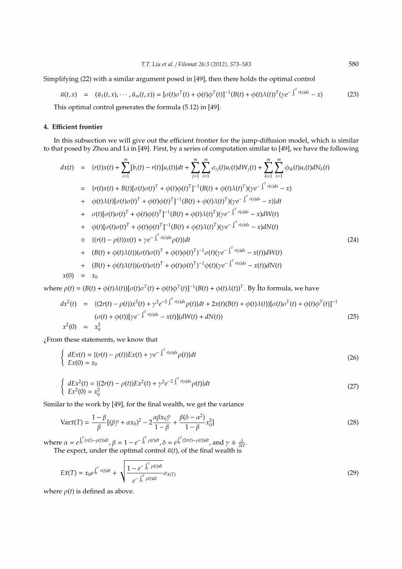
Simplifying (22) with a similar argument posed in [49], then there holds the optimal control

u(t, x) = (u1(t, x), · · · , um(t, x)) = [σ(t)σT(t) + ϕ(t)ϕT(t)]−1(B(t) + ϕ(t)λ(t))T(γe−∫ T

t r(s)ds − x) (23)

This optimal control generates the formula (5.12) in [49].

4. Efficient frontier

In this subsection we will give out the efficient frontier for the jump-diffusion model, which is similarto that posed by Zhou and Li in [49]. First, by a series of computation similar to [49], we have the following

dx(t) = r(t)x(t) +m∑

i=1

[bi(t) − r(t)]ui(t)dt +m∑

j=1

m∑i=1

σi j(t)ui(t)dW j(t) +m∑

k=1

m∑i=1

ϕik(t)ui(t)dNk(t)

= r(t)x(t) + B(t)[σ(t)σ(t)T + ϕ(t)ϕ(t)T]−1(B(t) + ϕ(t)λ(t)T)(γe−∫ T

t r(s)ds − x)

+ ϕ(t)λ(t)[σ(t)σ(t)T + ϕ(t)ϕ(t)T]−1(B(t) + ϕ(t)λ(t)T)(γe−∫ T

t r(s)ds − x)dt

+ σ(t)[σ(t)σ(t)T + ϕ(t)ϕ(t)T]−1(B(t) + ϕ(t)λ(t)T)(γe−∫ T

t r(s)ds − x)dW(t)

+ ϕ(t)[σ(t)σ(t)T + ϕ(t)ϕ(t)T]−1(B(t) + ϕ(t)λ(t)T)(γe−∫ T

t r(s)ds − x)dN(t)

+ (r(t) − ρ(t))x(t) + γe−∫ T

t r(s)dsρ(t)dt (24)

+ (B(t) + ϕ(t)λ(t))(σ(t)σ(t)T + ϕ(t)ϕ(t)T)−1σ(t)(γe−∫ T

t r(s)ds − x(t))dW(t)

+ (B(t) + ϕ(t)λ(t))(σ(t)σ(t)T + ϕ(t)ϕ(t)T)−1ϕ(t)(γe−∫ T

t r(s)ds − x(t))dN(t)x(0) = x0

where ρ(t) = (B(t) + ϕ(t)λ(t))[σ(t)σT(t) + ϕ(t)ϕT(t)]−1(B(t) + ϕ(t)λ(t))T. By Ito formula, we have

dx2(t) = (2r(t) − ρ(t))x2(t) + γ2e−2∫ T

t r(s)dsρ(t)dt + 2x(t)(B(t) + ϕ(t)λ(t))[σ(t)σT(t) + ϕ(t)ϕT(t)]−1

(σ(t) + ϕ(t))[γe−∫ T

t r(s)ds − x(t)](dW(t) + dN(t)) (25)x2(0) = x2

0

¿From these statements, we know thatdEx(t) = (r(t) − ρ(t))Ex(t) + γe−

∫ Tt r(s)dsρ(t)dt

Ex(0) = x0(26)

dEx2(t) = (2r(t) − ρ(t))Ex2(t) + γ2e−2

∫ Tt r(s)dsρ(t)dt

Ex2(0) = x20

(27)

Similar to the work by [49], for the final wealth, we get the variance

Varx(T) =1 − ββ

[(βγ + αx0)2 − 2αβx0γ

1 − β +β(δ − α2)

1 − β x20] (28)

where α = e∫ T

0 (r(t)−ρ(t))dt, β = 1 − e−∫ T

0 ρ(t)dt, δ = e∫ T

0 (2r(t)−ρ(t))dt, and γ + λ2H .

The expect, under the optimal control u(t), of the final wealth is

Ex(T) = x0e∫ T

0 r(t)dt +

√√1 − e−

∫ T0 ρ(t)dt

e−∫ T

0 ρ(t)dtσx(T) (29)

where ρ(t) is defined as above.

T.T. Liu et al. / Filomat 26:3 (2012), 573–583 581

Example 4.1. Suppose that there is a market risk-free security, the average annual return rate is r = 5%,there also is a stock with the average annual return rate is b = 15% and the standard fluctuation rate isσ = 16%. Assuming the magnitude of each jump is 1, that is ϕ = 1, the intensity of jumps is 1, that is λ = 1.Set T = 1 (one year) and ρ = (b−r+1)2

σ2+ϕ2 = 1.179797.

By a direct computation, we get the security market line

Ex(1) = x0e∫ 1

0 r(t)dt +

√√1 − e−

∫ 10 ρ(t)dt

e−∫ 1

0 ρ(t)dtσx(1) = x0e0.05 + 1.501238σx(1)

Assume now there is an investor who has initial assets x0 = 100, the expected return rate is 18% after oneyear, then we can calculate how much risk that the investor bear under the expected revenue.

By the security market line, when x0 = 100 and Ex(1) = 118, then we arrive at

σx(1) =Ex(1) − x0e0.05

1.501238=

118 − 100e0.05

1.501238= 8.574852

The result shows that the standard deviation of investor’s target is 8.574852%.Next, we calculate the investor’s portfolio as follows

γ =Ex(T) − αx0

β=

118 − 100e−1.022

1 − e−1.072 = 123.7118

Therefore, the investor’s asset invested in risky securities is

u(t, x(t)) = [σ(t)σT(t) + ϕ(t)ϕT(t)]−1(B(t) + ϕ(t)λ(t))T(γe−∫ T

t r(s)ds − x) = 1.072(123.7118e0.05(t−1) − x(t))

In the initial time t = 0, u(0, x0) = 18.96076, this implies that one can buy the risky security with his initialassets without borrowing additional money.

Excluding the occurrence of jumps, that is, we use the general diffusion model to describe fluctuationsof the market price, at the same time there is a risk-free security, the average annual return rate is r = 5%,there is an stock, its average annual return rate is b = 15% and the standard fluctuation rate is σ = 16%, setT = 1, then there holds

ρ1(t) =(b(t) − r(t))2

σ2(t)=

(0.15 − 0.05)2

0.162 = 0.3906

Ex1(1) = x0e∫ 1

0 r(t)dt +

√√1 − e−

∫ 10 ρ1(t)dt

e−∫ 1

0 ρ1(t)dtσx1(1) = x0e0.05 +

√1 − e−0.3906

e−0.3906 σx1(1) = x0e0.05 + 0.6912σx1(1)

Suppose that an investor has a initial asset x0 = 100, the expected return rate is 18% after one year, let’scalculate how much risk at this expected level. By Ex1(1) = x0e0.05 + 0.6912σx1(1), there is

σx1(1) =Ex1(1) − x0e0.05

0.6912= 18.6240

This shows that the expected standard deviation of the investor is 18.6240%. Now, we look at his portfoliochoice. Since

γ =118 − 100e0.05−0.3906

1 − e−0.3906 = 144.9604

then we get

u1(t, x) =(b(t) − r(t))2(γe−

∫ Tt r(s)ds − x)

σ21(t)

=0.01(144.9604e−0.05 − x)

0.162 = 0.3906(144.9604e0.05(t−1) − x)

T.T. Liu et al. / Filomat 26:3 (2012), 573–583 582

Considering the case t = 0, then one gets u1(0, x) = 14.80, this result shows that the investor should loan14.80 (yuan) at the initial time with his own initial principal 100 (yuan) all to invest in risky securities.Compare to the results under the two models, showing that when the asset price volatility in the marketcontains jumps, the investor will bear a larger bit of risks under the same expected revenue.

Acknowledgments

The authors would like to thank the referee for the revised opinion. The authors would also like tothank Professors Z. Li, X. Yang for their encouragement and guidance. This work was supported bythe Foundation of Nanjing University of Science and Technology and the Natural Science Foundations ofProvince, China.

References

[1] B. D. O. Anderson, J. B. Moore, Optimal Control-Linear Quadratic Methods, Prentice-Hall, Englewood, Cliffs, NJ, 1989.[2] F. Bao, P. Zhu, P. Zhao, Portfolio selection problems based on Fuzzy interval numbers under the Minimax rules, International J.

of Mathematical Analysis 4 (2010) 2143–2166.[3] A. Bensoussan, Lecture on stochastic control, part I. In: Nonlinear Filtering and Stochastic Control, Mitter SK, Moro A (eds),

Lecture Notes in Mathematics, Springer-Verlag, Berlin, 972 (1982) 1–39.[4] A. H. Y. Chen , F. C. Jen, S. Zionts, The optimal portfolio revision policy, Journal of Business 44 (1971) 51–61.[5] S. Chen, X. Li, X. Y. Zhou, Stochastic linear quadratic regulators with indefinite control weight costs, SIAM J. Control Optim. 36

(1998) 1685–1702.[6] S. Chen, X. Y. Zhou, Stochastic linear quadratic regulators with indefinite control weight costs, II. to appear in SIAM J. Control

Optim.[7] X. Deng, Y. Zhang, P. Zhao, Portfolio optimization based on spectral risk measures, International Journal of Mathematical

Analysis 3 (2009) 1657–1668.[8] D. Duffie, H. Richardson, Mean-variance hedging in continuous time, Ann Appl Probab. 1 (1991) 1–15.[9] B. Dumas, E. Liucinao, An exact solution to a dynamic portfolio choice problem under transaction costs, J. of Finance 46 (1991)

577–595.[10] E. J. Elton, M. J. Gruber, Finance as a Dynamic Process, Prentice-Hall, Englewood Cliffs, NJ, 1975.[11] E. F. Fama, The behavior of stock prices, Journal of Business 37:1 (1965) 34–105.[12] W. H. Fleming, H. M. Soner, Controlled Markov Processes and Viscosity Solutions, Springer-Verlag, New York, 1993.[13] H. Follmer, D. Sondermann, Hedging of non-redundant contingent claims, In: Contributions to Mathematical Economics,

Mas-Colell A, Hildenbrand W (eds). North-Holland, Amsterdam, 1986, 205–223.[14] J. C. Francis, Investments: Analysis and Management, McGraw-Hill, New York, 1976.[15] X. Guo, Y. Hu, P. Zhao, Portfolio selection problems based on generalized CVaR, Adv. Appl. Math. Sci. 1 (2009) 323–334.[16] R. R. Grauer, N. H. Hakansson, On the use of mean-variance and quadratic approximations in implementing dynamic investment

strategies: a comparison of returns and investment policies, Management Sci. 39 (1993) 856–871.[17] N. H. Hakansson, Multi-period mean-variance analysis: toward a general theory of portfolio choice, J. of Finance 26 (1971)

857–884.[18] B. Hou, J. Liu, P. Zhao, The evaluation of policy of portfolio problems, Appl. Math. Sci. 3 (2009) 2021–2034.[19] R. E. Kalman, Contributions to the theory of optimal control, Bol Soc Mat Mexicana 5: 102-119 Continuous-Time Portfolio

Selection 33, 1960.[20] M. Kohlmann , X. Y. Zhou, Relationship between backward stochastic differential equations and stochastic controls: an LQ

approach, to appear in SIAM J. Control Optim.[21] D. Li, W. L. Ng, Optimal dynamic portfolio selection: multi-period mean-variance formulation, to appear in Math. Finance.[22] A. E. B. Lim, X. Y. Zhou, Mean-variance portfolio selection with random parameters, Preprint, 1999.[23] J. Lintner, The valuation of risk assets and the selection of risky investments in stock portfolios and capital budgets, Review of

Economics and Statistics 47 (1965) 13–37.[24] D. G. Luenberger, Investment Science, Oxford University Press, New York, 1998.[25] H. Markowitz, Portfolio selection, J. of Finance 7 (1952) 77–91.[26] H. Markowitz, Portfolio Selection: Efficient Diversification of Investment, Wiley, New York, 1959.[27] R. C. Merton, Lifetime portfolio selection under uncertainty: the continuous time case, Review of Economics and Statistics 51

(1969) 247–257.[28] R. C. Merton, Optimal consumption and portfolio rules in a continuous-time model, Journal of Economic Theory 3 (1971) 373–413.[29] R. C. Merton, An analytic derivation of the efficient portfolio frontier, J. Finance Quant. Anal. 7 (1972) 1851–1872.[30] R. C. Merton, An intertemporal capital asset pricing model, Econometrica 41:5 (1973) 867–887.[31] J. P. Monique, M. Pontier, Optimal portfolio for a small investor in a market model with discontinuous prices, Applied Mathe-

matics and Optimization 22 (1990) 287–310.[32] J. Mossin, Equilibrium in a capital asset market, Econometrica 34 (1966) 768–783.[33] J. Mossin, Optimal multiperiod portfolio policies, J. Business 41 (1968) 215–229.

T.T. Liu et al. / Filomat 26:3 (2012), 573–583 583

[34] L. Pan, P. Zhao, Dynamic portfolio choice problems with non-monotone utility functions, Appl. Math. Sci. 2 (2008) 1761–1772.[35] E. Pardoux, S. Peng, Adapted solution of backward stochastic equation, System Control Lett 14 (1990) 55–61.[36] A. Perold, Large-scale portfolio optimization, Management Sci. 30 (1984) 1143–1160.[37] S. R. Pliska, Introduction to Mathematical Finance, Blackwell, Malden, 1997.[38] S. A. Ross, The arbitrage theory of capital asset pricing, Journal of Economic Theory 13 (1976) 341–360.[39] P. A. Samuelson, Rational proof that properly anticipated prices fluctuate randomly, Industrial Management Review 6:2 (1965)

41–49.[40] P. A. Samuelson, Lifetime portfolio selection by dynamic stochastic programming, Rev. Econom. Statist. 51 (1969) 239–246.[41] M. Schweizer, Variance-optimal hedging in discrete time, Math. Oper. Res. 20 (1995) 1–32.[42] W. F. Sharpe, Capital asset prices: a theory of market equilibrium under conditions of work, Journal of Finance 19 (1964) 425–442.[43] D. J. White, Dynamic programming and probabilistic constraints, Oper. Res. 22 (1974) 654–664.[44] W. M. Wonham, On a matrix Riccati equation of stochastic control, SIAM J. Control. 6 (1968) 312–326.[45] X. Wu, M. Xia, P. Zhao, The generalized no-arbitrage analysis of frictional markets, Adv. Appl. Stat. Sci. 1 (2009) 251–262.[46] C. Yang, P. Zhao, The portfolio problem under the variable rate of transaction costs, Far East J. Appl. Math. 31 (2008) 231–244.[47] J. Yong, X. Y. Zhou, Stochastic Controls: Hamiltonian Systems and HJB Equations, Springer-Verlag, New York, 1999.[48] P. L. Yu, Cone convexity, cone extreme points, and nondominated solutions in decision problem with multiobjectives, J. Optim.

Theory Appl. 7 (1971) 11–28.[49] X. Y. Zhou, D. Li, Continuous-time mean portfolio selection: a stochastic LQ framework, Applied Mathematics & Optimization

42 (2000) 19–33.