Embed Size (px)
Citation preview

PORTFOLIO OPTIMIZATION WITH MANY ASSETS:
THE IMPORTANCE OF SHORT-SELLING
Moshe Levy* and Yaacov Ritov **
May 2001
* School of Business Administration, The Hebrew University of Jerusalem, Jerusalem 91905,Israel. Tel: 972 2 5883219. Fax: 972 2 588 1341. [email protected]. On leave at UCLAAnderson School of Management, 110 Westwood Plaza, LA. CA. [email protected].
** Department of Statistics, The Hebrew University of Jerusalem, Jerusalem 91905, [email protected].

PORTFOLIO OPTIMIZATION WITH MANY ASSETS:
THE IMPORTANCE OF SHORT-SELLING
ABSTRACT
We investigate the properties of mean-variance efficient portfolios when the number
of assets is large. We show analytically and empirically that the proportion of assets
held short converges to 50% as the number of assets grows, and the investment
proportions are extreme, with several assets held in large positions. The cost of the
no-shortselling constraint increases dramatically with the number of assets. For about
100 assets the Sharpe ratio can be more than doubled with the removal of this
constraint. These results have profound implications for the theoretical validity of the
CAPM, and for policy regarding short-selling limitations.
Keywords: portfolio optimization, short-selling, CAPM.
JEL Classification: G11, G12, G18.
1
I. Introduction
The Capital Asset Pricing Model (CAPM), which was developed by Sharpe
[1964], Lintner [1965a], and Mossin [1966], is one of the cornerstones of modern
finance. The CAPM is founded on Markowitz’s mean-variance framework and on the
assumptions of homogeneous expectations and no limitations on short-selling. Based
on these (and other) assumptions, the CAPM derives a simple linear relation between
risk and return, and predicts that the optimal mean-variance portfolio should coincide
with the market portfolio.
As the CAPM allows for short-selling, it is possible, in principle, that the
optimal mean-variance portfolio involves short positions in some stocks. However,
this is in contradiction with the model’s prediction that the optimal portfolio should
coincide with the market portfolio. Thus, for the CAPM to be self-consistent, one
must ensure that the optimal portfolio does not involve short positions. Indeed, several
researchers attack this important problem by characterizing conditions that guarantee
efficient portfolios with no short positions. Roll [1977] provides conditions which
ensure that all positions in the global minimum-variance portfolio are positive (see
also Rudd [1977]). Roll and Ross [1977] later show that while these conditions are
sufficient, they are not necessary. Although Roll and Ross conclude that “…the
prospect appears dim for general and useful qualitative results” (p. 265), by
employing duality theory Green [1986] succeeds in finding general conditions
ensuring the existence of a mean-variance efficient portfolio with no short positions.
While Green’s conditions are intuitively appealing, empirical studies find that
in typical mean-variance efficient portfolios many assets are held short. For example,
Green and Hollifield [1992] compute the global minimum-variance portfolio for

2
different sets of 10 assets with empirically estimated parameters. They find that of the
90 sets of assets examined, 89 of the global minimum-variance portfolios involve
short positions. Levy [1983] constructs the efficient frontier for a set of 15 stocks. He
finds that throughout the efficient frontier 7-8 stocks, which constitute about 50% of
the assets in the portfolio, are held short.1 While several researchers suggest that these
results may be due to measurement errors in the estimation of the assets’ means and
the covariance matrix (see, for example, Frost and Savarino [1986], [1988])2, Levy
shows that his results are robust even when he takes possible estimation errors into
account, and when various estimation methods are employed. Are Levy’s results
coincidental, or are they general? If they are general, what is the reason for this result?
Obviously, if it is a general result that a large proportion of the assets are held short in
the mean-variance optimal portfolio, this constitutes a severe blow to the CAPM.
If the optimal mean-variance portfolio involves extensive short positions, this
not only questions the self-consistency of the CAPM, but may also have very
important practical policy implications. As many institutional investors are not
allowed to hold short positions (either through explicit regulations or by the implicit
threat of lawsuits), they are restricted to holding sub-optimal portfolios. How sub-
optimal are these portfolios? In other words, what is the cost of the no-short
restriction? (in terms of the Sharpe ratio, for example).
In this paper we empirically and theoretically investigate the properties of
mean-variance efficient portfolios in markets with a large number of assets. Our main
1 This is also consistent with the results of Pulley [1981], Kallberg and Ziemba [1983], and Kroll,Levy, and Markowitz [1984]. Jagannathan and Ma [2001] report similar results for the global minimumvariance portfolio.
2 See also Ledoit [1996], [1999] and Ledoit and Santa Clara [1998] for a discussion of covariancematrix estimation.

3
results are:
(1) When the number of assets is large, the proportion of assets held short in mean-
variance efficient portfolios typically converges to 50%.
(2) The investment proportions are extreme: a small number of assets are held in
large positions (long or short). (This is consistent with the findings of Green and
Hollifield [1992]).
(3) The investment proportion in each stock is not directly related to any of the
stock’s intrinsic properties such as its mean, variance, or its average correlation
(or covariance) with the other stocks. Rather, it depends on the exact composition
of the market.
(4) The cost of the no-shortselling constraint is extremely high. For portfolios with
many assets, the Sharpe ratio can be more than doubled by relaxing this
constraint.
Result (1) implies that the optimal mean-variance portfolio can not coincide with
the market portfolio, and therefore the CAPM can not be self-consistent. This problem
is different in essence than previous criticisms of the CAPM, such as its testability
(Roll [1977])3, or the validity of its underlying assumptions (in particular the
homogeneous expectation assumption, see Levy [1978], Merton [1987], and
Markowitz [1991]). Result (1) implies that even if the model’s assumptions do hold
perfectly, in large markets the CAPM can not possibly hold because of this theoretical
3 See also the discussion in Roll and Ross [1994] and Kandel and Stambaugh [1995].

4
internal inconsistency4. While there is an ongoing debate as to the empirical validity
of the CAPM (see, for example, Lintner [1965c], Black, Jensen, and Scholes [1972],
Miller and Scholes [1972], Levy [1978], Amihud, Christensen and Mendelson [1992],
Fama and French [1992], and Jagannathan and Wang [1993]), according to result (1)
the CAPM can not hold even in theory. Result (2) implies that the optimal mean-
variance portfolio is very different than portfolios constructed by “naive
diversification” strategies, such as the 1/n heuristic described by Benartzi and Thaler
[2001]. Thus, naive diversification may be very sub-optimal; the theory of portfolio
optimization is therefore of great practical importance. Result (3) implies that there is
no straightforward way to characterize a stock as “good” or “bad” in the context of
large portfolios. Even if a stock has a high expected return, a low variance, and a low
average correlation with all other stocks, when the number of assets is large, there is
no guarantee whatsoever that this stock will be held long in the optimal portfolio.
Result (4) implies that the restriction on short-selling is extremely costly. This result
has very important implications for policy-makers setting the regulations concerning
short-selling.
The structure of the paper is as follows: The next section describes empirical
results about mean-variance efficient portfolios. We find that approximately half of
the assets are held short, and that investment proportions are extreme. Moreover, it is
difficult to explain the proportion of a stock in the optimal portfolio in terms of any
4 Of course, to avoid this problem one can find the efficient frontier and the optimal portfolio under therestriction of no shortselling. However, in this case the problem becomes analytically complicated andone needs to employ the critical-line algorithm developed by Markowitz [1956], [1987] (see also Elton,Gruber, and Padberg [1976], [1978], Alexander [1993], and Kwan [1997]). More importantly, whenshort-selling is not allowed the CAPM’s linear risk-return relationship breaks down (see Markowitz[1990], Tobin [1990], and Sharpe [1991]). Our results are derived for general sets of parameters, thus,one could argue that the equilibrium parameters are endogenously determined by prices such that theoptimal portfolio weights are all positive. In section V we show that this approach can not ensurepositive portfolio weights, and therefore does not solve the CAPM’s internal inconsistency problem.

5
simple characteristic of the stock. The cost of the no-short-sell constraint is analyzed
in terms of the Sharpe ratio. Section III provides an intuition and a mathematical
explanation for the results. Section IV discusses the robustness of the results to
estimation errors. Section V concludes and discusses the implications of the results to
the theoretical validity of the CAPM, and to policy-making regarding limitations on
short-selling.
II. Empirical Properties of Mean-Variance Efficient Portfolios
In this section we describe the main properties of empirical mean-variance
efficient portfolios. We conduct this analysis by estimating the assets’ parameters
from the Center for Research in Security Prices (CRSP) monthly returns file, from the
period January 1979 to December 1999. We randomly selected firms from the set of
all CRSP firms, and then retained 200 of those firms selected with complete records
over the entire period.5 In our analysis we take the monthly risk-free rate as 0.32%
(for an annual rate of 3.9%, see Ibbotson [2000]). However, the results reported below
do not depend on the specific value of the risk-free rate. In this section we employ the
sample estimates and do not consider sampling errors or shrinkage methods. These
issues are discussed in section IV.
Result (1): Percentage of Assets Held Short
Figure 1 shows the percentage of stocks held short in the optimal portfolio as a
function of the number of stocks in the portfolio, N. For each N we randomly draw a
5 This is similar to the procedure employed by Green and Hollifield [1992]. However, as Green andHollifield construct portfolios of up to 50 stocks, they require only a five year period of completemonthly records (in order for covariance matrix estimated from historical data to be non-singular, thenumber of time periods over which returns are observed must exceed the number of assets). We take atwenty-year period because we construct portfolios of up to 200 stocks. While this introduces asurvivorship bias, we do not believe that this bias plays any significant role in our empirical analysis,and we obtain similar results in simulations where the expected returns and covariances are drawnrandomly from some distributions, as described in the next section, rather than estimated empirically.

6
sub-set of N stocks out of our set of 200 stocks, we calculate the mean-variance
optimal portfolio for this sub-set, and we record the number of assets held short in this
portfolio6. We repeat this 10 times for each N (each time with a different sub-set of N
stocks). Figure 1 reports the average proportion of stocks held short for each value of
N. As the figure shows, the percentage of stocks held short in the optimal portfolios
approaches 50% as the number of assets increases. This result is consistent with Levy
[1983], who finds that in his sample of stocks only 1 stock on average is held short
when the portfolio is constructed from 5 stocks, but when the portfolio is constructed
from 15 stocks 7-8 stocks are held short.
(Insert Figure 1 About Here)
Result (2): Extreme Investment Proportions
While result (1) shows that about 50% of the stocks are optimally held short,
we also find that some of these positions are rather extreme. We calculate the optimal
mean-variance portfolio for the set of all of the 200 stocks and construct the
distribution of portfolio weights. Figure 2 reports this distribution. The heavy line is
the empirical distribution7. The light line is the best normal fit. As Figure 2
demonstrates, the normal distribution is a very good approximation for the
6 Different assumptions regarding the terms of short selling are made by different models. The originalCAPM, as well as Black [1972] and Merton [1972] assume that the short seller does not have to put upany initial margin and can use the short proceeds. Lintner [1965b] suggests that an amount of moneyequal to the short proceeds is put up as margin, with the short seller receiving the riskfree interest rateon both the short proceeds and the margin. He shows that when borrowing is allowed this framework isidentical to having no margin requirements in terms of portfolio optimization. Dyl [1975] assumes thatthe short seller puts up initial margin that is less than the short proceeds, but receives no interest on themargin or on the short proceeds. Here we adopt the framework of the original CAPM, Lintner, Black,and Merton, for the sake of simplicity. See Markowitz [1987], Price [1989] and Weiss [1991] for adescription of shortselling procedures in practice, and Alexander [1993] for an excellent review ofalternative modeling assumptions and a unifying modeling framework for shortselling.
7 The empirical distribution is obtained by employing a non-parametric density estimate with aGaussian kernel and the "normal reference rule," (see Scott 1992, pg. 131).

7
distribution of optimal portfolio weights. This distribution implies that while most
stocks are held in small proportions, a few stocks are held in very large positions
(both long and short). This result is consistent with the findings of Green and
Hollifield who analyze the portfolio weights in empirical minimum-variance
portfolios. For portfolios of 50 assets they report an average absolute value of
portfolio weights of up to 24%(!) (while “naive” diversification leads to weights of
only 2%). The finding of extreme portfolio weights is in sharp contrast to notions of
“naive” diversification.
(Insert Figure 2 About Here)
Result (3): Portfolio Weight and Stock Characteristics
What determines which stocks are held long and which are shorted in the
optimal portfolio? In other words, what are the characteristics of a “good” stock,
which one would like to hold long in the portfolio? While it is well-known that when
stocks are correlated the optimal weight of each stock is affected by the parameters of
all the other stocks (for example, see Merton [1972], Levy [1973], Roll [1977], and
Stevens [1998]), it would seem intuitive that high mean return, low variance, and low
correlations with the other stocks are desirable characteristics, and that stocks with
these characteristics will tend to be held long. While this intuition may be helpful for
small portfolios, when considering portfolios of many assets this intuition is
misleading. When the number of assets in the portfolio is large, the very large number
of cross-interactions are dominant, and there is no simple way to characterize “good”
stocks, or to predict which stocks will have positive weights. Figure 3a shows the
relationship between stocks’ expected returns and their portfolio weights, in the mean-
variance optimal portfolio of the 200 stocks. There is no clear relationship between

8
expected return and portfolio weight. Similarly, Figure 3b shows that low standard
deviation does not imply positive portfolio weight. It is interesting to note, though,
that small standard deviation generally implies more extreme positions in the stock
(positive or negative). Finally, as Figure 3c shows, even average correlation with the
other stocks is not related to the optimal portfolio weight (nor is the average
covariance). While the figures show that the optimal investment proportion does not
seem related to expected return, standard deviation, or average correlation when each
of these factors is considered separately, one may suspect that a combination of these
three factors may better explain the portfolio weight. However, multivariate
regression of portfolio weight on these three variables reveals an 2R of only 0.042
(adjusted 2R of 0.027).
(Insert Figure 3 About Here)
Result (4): The Cost of the No-Shortselling Constraint
While the optimal mean-variance portfolio in a market with many assets involves
short positions in about 50% of the assets, one may argue that this result is not
necessarily significant in an economic sense, because it may be possible that there is a
portfolio with no short positions which is only slightly sub-optimal. In order to
address this issue of the economic cost of the short-selling restriction we calculate the
Sharpe ratio of the mean-variance optimal portfolio (with shortselling), and compare
it with the Sharpe ratio of the optimal portfolio constructed from the same assets, but
under the restriction of no shortselling. We make the Sharpe ratio comparison for
various portfolio sizes, N, where N is the number of assets in the portfolio. For each N
we randomly select N stocks out of the 200 stocks, and we calculate the optimal

9
portfolios with and without shortselling, and their Sharpe ratios. Figure 4 reports the
results.
(Insert Figure 4 About Here)
For portfolios with relatively few stocks, the difference in the Sharpe ratios is
not very big, consistent with Sharpe’s observation regarding the no-shortselling
constraint that “… magnitudes of the departures from the implications of the original
CAPM might be small” (see Sharpe [1991], p. 505). However, as the number of assets
in the portfolio increases, the Sharpe ratio of the unrestricted portfolios grows at an
almost steady rate, while the Sharpe ratio of the portfolios with the no-shortsell
constraint almost levels off. For portfolios of a little over 100 stocks the Sharpe ratio
can be more than doubled by removing the no-shortsell constraint. This is clearly a
tremendous economic difference.
III. Explanation of the Results
This section provides a mathematical and intuitive explanation for the empirical
results reported in previous studies and in the preceding section. These results are
shown to be a general property of mean-variance optimal portfolios when the number
of assets is large. Graphical analysis may provide some insight and intuition. Figure 5
shows Markowitz’s mean-variance plane, and the efficient frontier derived for a set of
N stocks. Now, suppose that we add a new stock, stock N+1. One can think of the
possible portfolios of the N+1 stocks as combinations of portfolios of the N “old”
stocks and the new stock. In order for the new stock to have a non-zero portfolio
weight in any efficient portfolio, one of these combinations must improve the “old”
efficient frontier. However, notice that if no shortselling is allowed and most
covariances are positive, combinations of the new stock with existing portfolios are
most likely to be interior to the frontier (see solid lines in Figure 5). Thus, if no

10
shortselling is allowed and there are many assets in the market, adding one more asset
does not typically extend the efficient frontier, and the weight of this newly added
stock in efficient portfolios will typically be 0. This is consistent with the results of
Figure 4, showing that when shortselling is not allowed, at some stage the Sharpe
ratio almost does not increase as more stocks are being added.
(Insert Figure 5 About Here)
However, when shortselling is allowed, the situation is very different. In this case,
one can extend the efficient frontier by considering combinations of the new stock
with other portfolios, in which either the new stock, or the portfolio of “old” stocks
are held short. As Figure 5 shows, for a “typical” stock both cases are similarly likely
(see dotted lines). Thus, for a given riskfree rate, we would expect that every newly
added stock has roughly the same probability of being positively or negatively
weighted. Hence, when the number of stocks is large, we can expect efficient
portfolios to have about half of the stocks held short, as indeed observed in Figure 1.
For a mathematical explanation of the empirical findings described in the previous
section, one has either to assume a specific covariance matrix, or alternatively to
derive statistical results for certain covariance matrix classes. In what follows we take
both approaches. First, we analyze the equal pairwise correlation case advocated by
Elton and Gruber [1973] and Schwert and Seguin [1990], and we prove that this
covariance structure generally leads to about half of the assets being held short and to
extreme portfolio weights. In the second approach we consider covariance matrices
drawn at random from some ensemble, and prove that the Sharpe ratio increases
indefinitely with the number of assets when shortselling is allowed, but levels-off
when shortselling is not allowed.

11
Equal Correlations
Consider the Elton-Gruber [1973] case in which all pairwise correlations are
identical. For simplicity, assume first that all variances are identical. For N stocks, the
covariance matrix in this case is an NxN matrix with 2σ on the diagonal and
2ρσ elsewhere. The inverse of this matrix is 22 )1N()2N(1)2N(11a
ρ−−ρ−+ρ−+
σ= on the
diagonal, and 22 )1N()2N(11b
ρ−−ρ−+ρ−
σ= elsewhere. Denoting excess returns
by µ , the (unscaled) investment proportion of stock i in the optimal portfolio is:
µ+µ−=∑ µ+µ=ω≠=
Nb)ba(ba in
ij1j
jii , where ∑µ=µ=
N
1jjN
1 is the mean value of the
assets’ expected returns (for the scaled proportions one has to divide iω by ∑=
n
1jjω ).
Writing a and b explicitly, we find that an asset is held short if )N/)1((1i ρρ−+
µ<µ .
For small values of N this condition may not hold for any of the assets. However,
when the number of assets is large, each stock is held short if its expected return is
slightly smaller than the average expected return µ (and held long if it is larger than
this average). If the distribution of excess returns is not very skewed, this implies that
about half of the stocks are held short in the optimal portfolio. Notice that this result
holds for any value of the correlation ρ , as long as it is not 0 or 1.
In addition, the portfolio weights are extreme in the sense that they do not become
smaller as the number of assets increases. To see this, recall that the scaled portfolio

12
weights are given by ∑ω
ω
=
n
1jj
i . As ∞→N iω converges to )1(2
i
ρ−σµ−µ . The denominator,
∑ω=
n
1jj , converges to
ρσµ2 . Thus, the scaled portfolio weight of asset i converges to
ρ−ρ
µµ−µ
1i , and does not get small even when the number of assets becomes very
large. For example, if 5.0=ρ and a stock has an expected return 20% higher than the
average expected return, this stock will have a weight of 20% in the optimal portfolio,
even if there are thousands of other stocks in the portfolio.
In the case where stocks have different variances, the arguments are very similar.
In this case the covariance matrix can be written as:
=
n
2
n
2
000
00
1
11
000
00
C
σ
σσ
ρρρ
ρρρ
σ
σσ
L
MO
M
L
L
MOM
L
L
MO
M
L
and when N is large stock i will be held short if ∑≠=−
<n
ij1j j
j
i
i
1n1
σµ
σµ . Again, if the
distribution of σµ is not very skewed, we would expect about half of the assets to be
held short8.
Kandel [1984] shows that for any set of N-1 assets one can mathematically
construct an Nth asset such that the mean-variance optimal portfolio is positively
8 As σ is bounded by 0, if the distribution of
σµ is skewed, it is probably positively skewed, implying
that even more than 50% of the assets will be held short.

13
weighted (see Theorem 1, p. 67 in Kandel [1984], and Green and Hollifield [1992] p.
1066). While such an Nth asset always exists mathematically, in large markets this
asset may be very a-typical and unrealistic. To see this, consider the 200 assets
randomly selected from the CRSP file as described in section II. What are the
characteristics of the 201st asset which makes the optimal portfolio positively
weighted (say, with an investment proportion of 1/201 in each asset)? Following the
procedure in Kandel for characterizing this asset (p. 67), we find that the added asset
should have a monthly standard deviation of at least 642%.9 The expected monthly
return of this asset is 64,020% (!). Thus, while it is always possible to mathematically
construct an Nth asset which makes the optimal portfolio positively weighted, this
does not imply that it is reasonable to expect the existence of a positively weighted
optimal portfolio for a general (or empirical) set of parameters.
Random Covariance Matrix Analysis
Obviously, any specific set of covariances and expected returns determines a
specific set of optimal portfolio weights. However, one can derive general properties
of optimal portfolios by making some assumptions on the space of covariance
matrices and taking a statistical approach10. Namely, one can assume that
covariance matrices are drawn randomly from some ensemble, and derive statistical
results regarding optimal portfolio weights. This approach is commonly employed in
physics when one is not interested (or does not know) the parameters of a specific
system, but rather one tries to make a statement about the properties of “typical”
9 As Kandel shows, the added Nth asset is not unique. We report here the added 201st asset with theminimal possible standard deviation. The other possibilities involve even more extreme parameters.
10 Longstaff, Santa-Clara, and Schwartz [2001a, 2001b] recently employ a similar approach toinvestigate the covariance structure among forwards.

14
systems of a certain type (see, for example, Wigner [1951], Carmeli [1983], and
Mehta [1991]). Below we conduct such an analysis to show that the Sharpe ratio
increases indefinitely with the number of assets when shortselling is allowed, but
levels-off when shortselling is not allowed (as found empirically and reported in
Figure 4). We would like to stress that while Theorem 1 below assumes a certain
covariance structure, extensive numerical analysis indicates that the results are quite
general.
Theorem 1:
Consider an NN × covariance matrix given by: += MC '11α , where M is a
standard Wishart matrix with d<N degrees of freedom, 1 is a vector of 1’s, and α is a
positive constant. Let the vector of excess returns be non-degenerate. As the number
of assets grows to infinity ( ∞→N ) the Sharpe ratio grows indefinitely when
shortselling is allowed, but levels-off when shortselling is not allowed.
Comment 1: The Wishart matrix M can be written as X'X , where X is a Nd × matrix
with random N(0,1) elements. This construction implies a linear factor structure (see,
for example, Carmeli [1983]).
Comment 2: α is the average covariance.
Comment 3: M is symmetric positive definite, and therefore so is C.
Proof:
Denote the vector of excess returns by µ . If shortselling is allowed, the unscaled
optimal investment proportions vector, ω , is given by µ1C− (the scaled proportions
are given by ω /( '1 ω ), see Merton [1972]; since we are deriving the Sharpe ratio, it
does not make a difference if one is working with the scaled or unscaled proportions).

15
The expected return is given by ωµ ' or µµ 1C' − . Notice, however, that µ can be
written as:
1)'1(MC ωαωωµ +== . (1)
Rearranging we have:
1)'1(M ωαµω −= . (2)
Multiplying by 1−M we obtain:
1M)'1(M 11 −− −= ωαµω , (3)
or: 1M'1)'1(M'1'1 11 −− −= ωαµω . (4)
Rearranging eq.(4) yields:
11M'1M'1'1 1
1
+= −
−
αµω (5)
Substituting this expression for ω'1 in eq.(3), we have:
1M11M'1
M'1M 11
11 −
−
−−
+−=
αµαµω . (6)
Thus, the expected return, µµ 1C' − or ωµ ' is given by: (7)
( )11M'1
M')M'1(1M'1M'11M'1
)M'1(M'' 1
12111
1
211
++−=
+−= −
−−−−
−
−−
αµµµµµα
αµαµµωµ .
Since the eigenvalues of the Wishart matrix M are bounded away from 0 and are
bounded from above (Silverstein [1986], Mehta [1991] p. 75), both expressions
µµ 1M' − and 1M'1 1− are of order N, where N is the number of assets (and dimension of
the vectors µ and 1). The difference 2111 )M'1(1M'1M' µµµ −−− − , which is positive
by the Schwartz inequality, is therefore of order 2N . Hence, the expected return
ωµ ' is of order N.

16
The standard deviation of the optimal portfolio is ωω C' . As µω 1C−= we
have:
=σ ωω C' = ωµ=µµ=µµ −−− 'C'CCC' 111 , (8)
which is the square root of the expression in eq.(7), and is therefore of the order of
N . Thus, when the number of assets, N, is large, and shortselling is allowed, the
Sharpe ratio is of order NN
N = , and it grows indefinitely with the number of
assets.
In contrast, if shortselling is not allowed, the Sharpe ratio levels off:
0max
>ωµ
αωαµω
ωαωωµω
ωωµω max1
'1'
)'1(M''
C''
2≤≤
+≤ . (9)
Q.E.D.
While the above analysis makes an assumption regarding the structure of the
covariance matrix, numerical simulations show that the results are very general, and
hold under a variety of other covariance structures. For example, Figure 6 displays the
results of numerical simulations in which the correlation between any two stocks is
drawn randomly from a uniform distribution. After the correlation matrix is drawn
this way, we check whether it is positive definite- if it is not we reject it and draw
another matrix. The results in Figure 6 are obtained with the following parameters:
ijρ is drawn from a uniform distribution on the segment [0.4, 0.5]11, the excess return
iµ is drawn from a uniform distribution on the segment [0, 0.2], and the standard
deviation iσ is drawn from a uniform distribution on the segment [0.2, 0.5]. As
11 We choose a relatively narrow range for the correlations, because otherwise, as the number of assetsbecomes large, it becomes increasingly difficult to generate positive definite matrices by the proceduredescribed above.

17
Figure 6 shows, the results we find empirically are also obtained in the simulation
analysis, and they are therefore not likely to be due to empirical estimation errors or to
a survivorship bias. Similar numerical results are obtained with various parameter
values and distributional assumptions.
(Insert Figure 6 About Here)
IV. Robustness to Estimation Error
The analysis up to this point, as well as the CAPM framework, assume that the
expected returns and covariances are known. In practice, however, these parameters
are not given, and have to be estimated, which typically involves some estimation
error. To what extent do the above results carry through when estimation error is
involved?
In order to deal with estimation errors it is common to employ shrinkage
estimators, or to impose portfolio weight constraints to avoid extreme positions. In a
recent innovative paper Jagannathan and Ma (2001) that these two approaches are in
fact very closely linked. The effect of employing portfolio weight constraints depends
on two main factors: the magnitude of the estimation error, and the difference in
performance between the optimal and the constrained portfolios with the “true”
parameters. If this performance difference is large, and the estimation errors are small,
imposing constraints is likely to hurt performance, and vice versa. Jagannathan and
Ma (2001) employ simulations to investigate the benefits of the constraints as a
function of the estimation error. Here we take a similar approach.
As shown in the preceding sections, when the number of assets is large, the
difference in performance between the optimal and the constrained portfolios with the
“true” parameters is very large. Hence for large portfolios we expect the
unconstrained portfolio to outperform the constrained portfolio even when substantial

18
estimation error is involved. We investigate this issue numerically by randomly
drawing a “true” covariance matrix and “true” excess returns as described in section
III. Then we create the “estimated” or observed parameters by adding estimation
error, or “noise”, to the true parameters. Specifically, we take
)~1(i0i µε+µ=µ (10)
)~1(i0i σε+σ=σ (11)
where µ and σ are the “true” parameters, the superscript 0 denotes the observed
parameters, and µε~ and σε~ are error terms which are normally distributed N(0, 2
εσ ),
and are independent of each other and across assets. Given the observed parameters,
the optimal portfolio weights, 0ω , (with and without shortselling) are derived. We
calculate the actual performance of the constructed portfolios by employing the “true”
parameters, in terms of the Sharpe ratio:
00
0
C'
'
ωω
µω .
The performance of the portfolios with and without shortselling as a function of the
estimation error εσ is described in Figure 7. The number of assets is 100, and the
Sharpe ratios reported are averaged over 10 independent simulations at each error
level. For comparison, the figure also describes the performance of a “naive”
diversification portfolio with a proportion 100
1 in each asset. For low error levels
( 0≈σε ) the observed parameters are close to the “true” parameters, and shortselling
dramatically increases the portfolio performance, as reported previously in Figures 4
and 6. As the error increases, the Sharpe ratio of both portfolios (with and without
shortselling) declines, and the advantage of shortselling also decreases, as reported in

19
Jagannathan and Ma. Notice, however, that even with a significant level of error (e.g.
%30=σε ) employing shortselling results in doubling the Sharpe ratio.
(Insert Figure 7 About Here)
V. Summary and Discussion
In this paper we investigate the properties of mean-variance efficient
portfolios in markets with a large number of assets and a general return and
covariance structure. Our main results are:
(1) The proportion of assets held short in mean-variance efficient portfolios
converges to 50% as the number of assets increases.
(2) The investment proportions are extreme: several assets are held in very large
positions (long or short).
(3) The investment proportion in each stock is not directly related to any simple
intrinsic characteristic of the stock such as its mean, variance, or its average
correlation (or covariance) with the other stocks. Thus, in the context of large
portfolios it is not straightforward to characterize a “good” stock.
(4) The cost of the no-shortselling constraint is extremely high. For large portfolios
the Sharpe ratio can be more than doubled by relaxing this constraint.
These results are obtained empirically under various estimation methods,
analytically, and in numerical simulations. Thus, the results seem to be fundamental
properties of mean-variance efficient portfolios in large markets.
The first result reveals a severe theoretical inconsistency of the CAPM. On the
one hand, the model predicts that the optimal mean-variance portfolio coincides with
the market portfolio; On the other hand, result (1) states that for large markets about
half of the assets are held short in the optimal portfolio, which means that the market

20
portfolio can not possibly coincide with the optimal portfolio. As Green and Hollifield
[1992] and Kandel [1984] show, there are conditions which ensure a mean-variance
efficient portfolio with no short positions. However, result (1) indicates that for large
markets these conditions may be very unlikely to hold.
One line of defense for the CAPM could be based on the notion that in
equilibrium prices are determined such that the optimal portfolio has all weights
positive. Specifically, according to Lintner’s approach to the CAPM companies’ end-
of-period value distributions are given, and market prices “adjust and readjust” until
in equilibrium the vector of asset prices yields a vector of expected returns and a
covariance matrix which lead to the linear SML relation between beta and expected
return (see Lintner [1965a] p. 598). Taking this approach, one may hope that the price
vector can be determined such that not only the SML holds, but in addition the
optimal portfolio is positively weighted. However, this line of defense is problematic
for at least two reasons. First, as Nielsen [1988] elegantly shows, Lintner’s approach
leads to the problem of multiple CAPM equilibria. In order to reduce the infinite set
of possible equilibria, specific preferences and initial endowments have to be
considered. However, this does not automatically ensure a unique equilibrium. Even
with specific assumptions regarding preferences and endowments one can have
multiple equilibria, a unique equilibrium, or no equilibrium at all. Second, even if
the preferences and endowments are such that there is a unique equilibrium, this does
not solve the more severe problem of short positions in the optimal mean-variance

21
portfolio.12 Thus, it seems that this line of defense does not save the model from its
internal inconsistencies. One promising avenue which may offer a solution to this
problem is the segmented market approach of Levy [1978], Merton [1987],
Markowitz [1990] and Sharpe [1991]. According to the segmented market approach
investors may hold only a limited number of assets due to transaction costs,
asymmetric information, or various biases. In this case each investor may hold several
assets short in his portfolio, while the market portfolio can have all positive weights.
The second and third results of this paper state that the optimal mean-variance
portfolio is very different from “naively diversified” portfolios. As the forth result
shows, this difference is economically very significance. This implies that naively
diversifying between many stocks or between several mutual funds (as many
investors do) is very sub-optimal. Thus, there is great practical and economic value to
the portfolio optimization taught to us by Markowitz.
The cost of the no-shortselling constraint depends on the magnitude of the
estimation error (Jagannathan and Ma [2001]), and on the number of assets. When the
number of assets is large the cost of this constraint may be tremendous. Although
12 For example, consider an economy with a single constant-absolute-risk-aversion investor with riskaversion parameter a. Given a riskfree rate r and a market portfolio with expected return mR and
variance 2mσ , such an investor optimally invests
arRT 2
m
m0 σ
−= dollars in the market portfolio. Lintner
[1965a] defines the market price of risk, γ , as 0
2m
m
TrR
σγ −= . Thus, a=γ , and in this case the market
price of risk is just the investor’s risk aversion parameter. To see that negative prices are possible inthis framework, assume, for example, a=2, and a market with a riskfree rate of 10% and two riskyassets with 5.0,2,4.0,10P,1P 122121 =ρ=σ=σ== , where all of these relate to end-of-period values(recall that in this framework the firms’ end-of-period value distributions are given, and today’s pricessimultaneously determine the expected returns and covariances). Let there be one share of each riskyasset. Employing Lintner’s formulas for equilibrium prices (Lintner, 1965a, eq.17 on pg. 600) with amarket price of risk of 2, we obtain a price of -$0.109 for asset 1, and $1.091 for asset 2. While it iscounter-intuitive to have an asset with a negative price, this results from the CAPM framework withnormal distributions, which implies that negative terminal values are possible.

22
short-selling may have a speculative and therefore risky connotation, used responsibly
in a large portfolio context it implies the exact opposite. Funds that are not allowed to
sell short because of “safety considerations” could reduce their risk by more than half
while maintaining the same expected return if they were allowed to sell short.
REFERENCES
Alexander, G. J., 1993, Short selling and efficient sets, Journal of Finance 48, 1497-1506.
Amihud, Y., B. J. Christensen and H. Mendelson, 1992, Further evidence on therisk-return relationship, working paper, Stanford University.
Benartzi, S. and R. Thaler, 2000, Naive diversification strategies in definedcontribution saving plans, American Economic Review, forthcoming.
Black, F., 1972, Capital market equilibrium with restricted borrowing, Journal ofBusiness 45, 444-454.
Black, F., M.C. Jensen, and M. Scholes, 1972, The Capital Asset Model: SomeEmpirical Tests, in Michael C. Jensen, ed., Studies in the Theory of CapitalMarkets, New York.
Carmeli, M., 1983, Statistical Theory of Random Matrices, Marcel Dekker, NewYork.
Dyl, E. A., 1975, Negative betas: The attractions of selling short, Journal of PortfolioManagement 3, 74-76.
Elton, E. J., and M. J. Gruber, 1973, Estimating the dependence structure of shareprices – implications for portfolio selection, Journal of Finance 28, 1203-1232.
Elton, E. J., M. J. Gruber, and M. W. Padberg, 1976, Simple criteria for optimalportfolio selection, Journal of Finance 31, 1341-1357.
Fama, E. and K. French, 1992, The cross-section of expected stock returns,Journal of Finance 47, 427-465.
Frost, P. A. and J. E. Savarino, 1986, An empirical Bayes approach to efficientportfolio selection, Journal of Financial and Quantitative Analysis 21, 293-306.
Frost, P. A. and J. E. Savarino, 1988, For better performance: Constrain portfolioweights, Journal of Portfolio Management 14, 29-34.
Green, R. C., 1986, Positively weighted portfolios on the minimum-variance frontier,Journal of Finance 41, 5, 1051-1068.
Green, R. C. and B. Hollifield, 1992, When will mean-variance efficient portfolios bewell diversified? Journal of Finance 47, 1785-1809.
Ibbotson Associates, 2000, Stocks, Bonds, Bills and Inflation, (Chicago, Illinois).

Jagannathan, R., and Z. Wang, 1993, The CAPM is alive and well, FederalReserve Bank of Minneapolis Staff Report 165.
Jagannathan, R., and T. Ma, 2001, Risk reduction in large portfolios: a role forportfolio weight constraints, Northwestern University working paper.
Kallberg, J. G. and W. T. Ziemba, 1983, Comparison of alternative utility functions inportfolio selection problems, Management Science 29, 1257-1276.
Kandel, S., 1984, On the exclusion of assets from tests of the mean varianceefficiency of the market portfolio, Journal of Finance 39, 63-75.
Kandel, S., and R. F. Stambaugh, 1995, Portfolio inefficiency and the cross-section ofexpected returns, Journal of Finance 50, 157-184.
Kroll, Y., H. Levy and H. Markowitz, 1984, Mean-variance versus direct utilitymaximization, Journal of Finance 39, 47-61.
Kwan, C. Y., 1997, Portfolio selection under institutional procedures for short selling:Normative and market-equilibrium considerations, Journal of Banking and Finance21, 369-391.
Ledoit, O., 1996, A well-conditioned estimator for large dimensional covariancematrices, UCLA working paper.
Ledoit, O., 1999, Improved estimation of the covariance matrix of stock returns withan application to portfolio selection, UCLA working paper.
Ledoit, O., and P. Santa-Clara, 1999, Estimating large conditional covariancematrices with an application to international stock markets, UCLA working paper.
Levy, H., 1973, The demand for assets under conditions of risk, Journal of Finance,28, 79-96.
Levy, H., 1978, Equilibrium in an imperfect market: a constraint on the number ofsecurities in the portfolio, American Economic Review 68, 643-658.
Levy, H., 1983, The capital asset pricing model: theory and empiricism, EconomicJournal 93, 145- 165.
Lintner, J., 1965a, Security prices, risk, and the maximal gains from diversification,Journal of Finance, 20(4), 587-615.
Lintner, J., 1965b, The valuation of risk assets and the selection of risky investmentsin stock portfolios and capital budgets, Review of Economics and Statistics 47, 13-37.
Lintner, J., 1965c, Security prices and risk: the theory of comparative analysis ofAT&T and leading industrials, paper presented at the conference on theeconomics of regulated public utilities, Chicago.

Longstaff, F., Santa-Clara, P., and E. Schwartz, 2001a, Throwing away a billiondollars: the cost of suboptimal exercise in the swaptions market, Journal ofFinancial Economics, forthcoming.
Longstaff, F., Santa-Clara, P., and E. Schwartz, 2001b, The relative valuation ofcaps and swaptions: theory and empirical evidence, Journal of Finance,forthcoming.
Markowitz, H., 1952, Portfolio selection, Journal of Finance 7, 77-91.
Markowitz, H., 1956, The optimization of a quadratic function subject to linearconstraints, Naval Research Logistics Quarterly 3, 111-133.
Markowitz, H., 1959, Portfolio Selection: Efficient Diversification of Investments,(John Wiley and Sons, Somerset, NJ).
Markowitz, H., 1987, Mean-Variance Analysis in Portfolio Choice and CapitalMarkets, (Basil Blackwell Inc., New York).
Markowitz, H., 1990, Risk adjustment, Journal of Accounting, Auditing and Finance,213-225.
Mehta, M.L., 1991, Random Matrices, Academic Press, Boston.
Merton, R. C., 1972, An analytic derivation of the efficient portfolio frontier, Journalof Financial and Quantitative Analysis 7, 1851-1872.
Merton, R. C., 1987, A simple model of capital market equilibrium with incompleteinformation, Journal of Finance 42, 483-510.
Mossin, J., 1966, Equilibrium in a capital asset market, Econometrica 35, 768-783.
Nielsen, L. T., 1988, Uniqueness of equilibrium in the classical CAPM, Journal ofFinancial and Quantitative Analysis 23, 329-336.
Price, K, 1989, Long on safety: don’t sell short selling short, Barron’s, November 6,16.
Pulley, L. B., 1981, General mean-variance approximation to expected utility forshort holding periods, Journal of Financial and Quantitative Analysis 16, 361-373.
Roll, R., 1977, A critique of the asset pricing theory’s tests; Part I: On past andpotential testability of the theory, Journal of Financial Economics 4, 129-176.
Roll, R. and S. A. Ross, 1977, Comments on qualitative results for investmentproportions, Journal of Financial Economics 5, 265-268.

Roll, R. and S. A. Ross, 1994, On the cross-sectional relation between expectedreturns and betas, Journal of Finance 49, 101-121.
Rudd, A., 1977, A note on qualitative results for investment proportions, Journal ofFinancial Economics 5, 259-263.
Schwert, G.W., and P. J. Seguin, 1990, Heteroskedasticity in stock returns, Journal ofFinance 45, 1129-55.
Scott, D. W., 1992, Multivariate Density Estimation, New York: Wiley.
Sharpe, W., 1964, Capital asset prices: a theory of market equilibrium underconditions of risk, Journal of Finance 19, 425-442.
Sharpe, W., 1966, Mutual fund performance, Journal of Business, 119-138.
Sharpe, W., 1991, Capital asset prices with and without negative holdings, Journal ofFinance 46, 489-509.
Silverstein, J.W., 1986, Eigenvalues and eigenvectors of large dimensional samplecovariance matrices, Contemporary Mathematics 59, 153—159.
Stevens, G., 1998, On the inverse of the covariance matrix in portfolio analysis,Journal of Finance 53, 1821-27.
Tobin, J., 1990, Discussion of risk adjustment, Journal of Accounting, Auditing andFinance, 229-234.
Weiss, G., 1991, The long and short of short-selling, Business Week, June 10, 106-108.
Wigner, E. P., 1951, On the statistical distribution of the widths and spacings ofnuclear resonance levels, Proceedings of the Cambridge Philosophical Society 47,790.

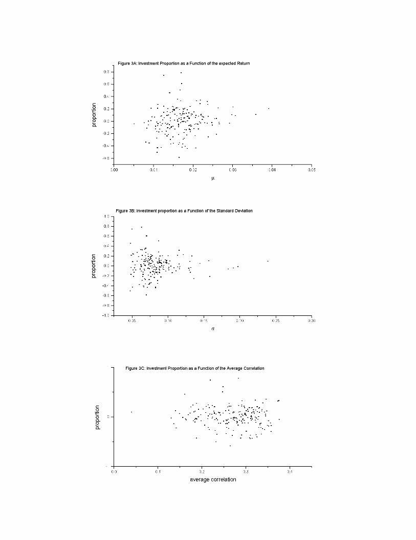

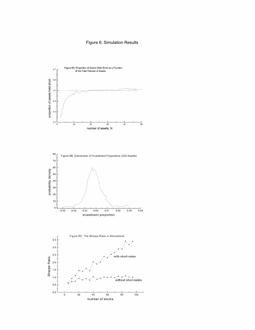
Figure 6: Simulation Results