Embed Size (px)
Citation preview

Portfolio Optimization Using
Conditional Value-At-Risk and Conditional Drawdown-At-Risk
Enn Kuutan
A thesis submitted in partial fulfillment of the degree of
BACHELOR OF APPLIED SCIENCE
Supervisor: Dr. R.H. Kwon
Department of Mechanical and Industrial Engineering
University of Toronto
March 2007

Portfolio Optimization Using CVaR and CDaR
i
ABSTRACT
Portfolio money management is an important concept because the amount of capital risked determines the overall profit and loss potential of a portfolio. Risk management methodologies assume some measure of risk impacts the allocation of capital (or position sizing) in a portfolio. The classical Markowitz theory identifies risk as the volatility or variance of a portfolio. Conditional Value-at-Risk (“CVaR”) and Conditional Drawdown-at-Risk (“CDaR”) are two risk functions that identify risk as portfolio losses and portfolio drawdowns, respectively. Mathematical models allow investors and portfolio managers to determine optimal asset allocation strategies. Linear programming techniques have become useful for portfolio rebalancing problems because of the effectiveness and robustness of linear program solving algorithms. Conditional Value-At-Risk and Conditional Drawdown-At-Risk are two risk measures that can be utilized in the portfolio linear programming model. A linear portfolio rebalancing model was developed and used to optimize asset allocation. The CVaR and CDaR risk measures were formulated for use in a linear programming framework. This framework was modeled in the ILOG OPL Development Studio IDE. Several portfolio allocations were created through the optimization of risk for both risk measures while ensuring that the portfolio return was constrained to a minimum level. Through an analysis of the portfolio allocation results, the CDaR risk measure was seen to be less stable than the CVaR risk measure. It was also determined that CDaR is a more conservative measure of risk than CVaR. Decreasing diversification coincided with an increase in portfolio risk and reward with both risk measures. Capital was allocated to assets with lower correlations to offset risk.

Portfolio Optimization Using CVaR and CDaR
ii
ACKNOWLEDGEMENTS
I would like to thank my thesis supervisor, Professor Roy Kwon. Without his ongoing
support and guidance, this thesis would not have been possible. I would also like to thank
my family and friends for their ongoing support throughout my university experience.
Portfolio Optimization Using CVaR and CDaR
iii
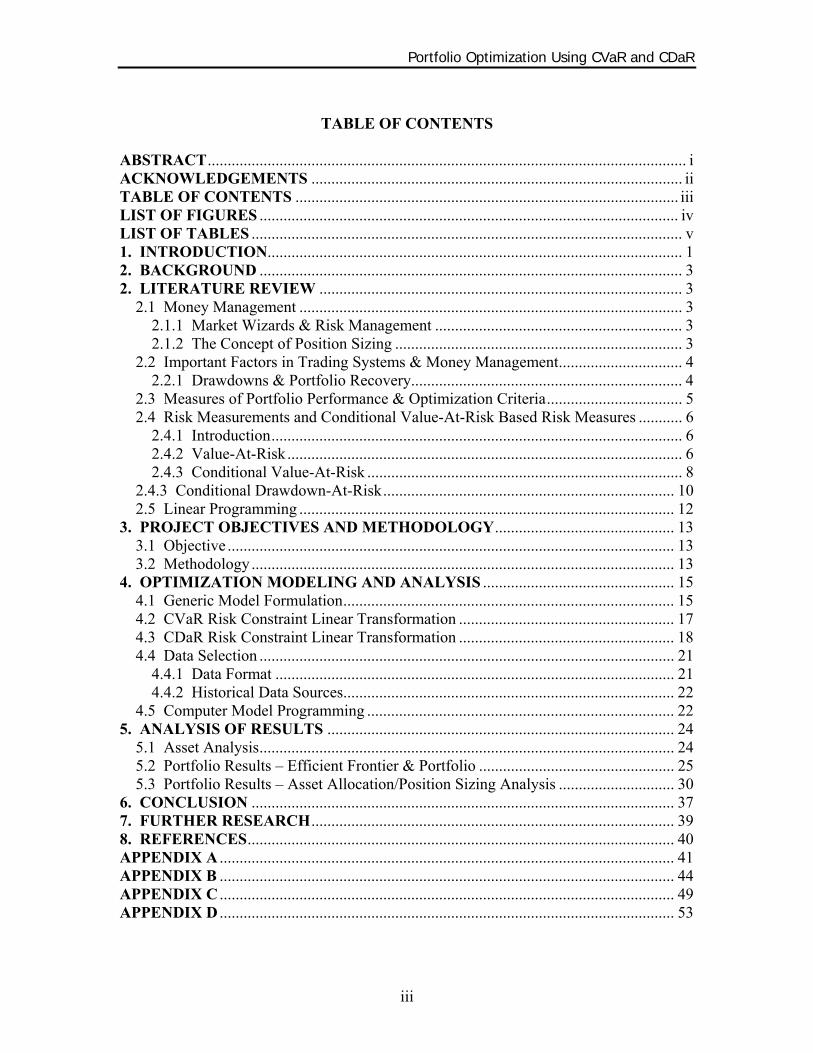
TABLE OF CONTENTS
ABSTRACT........................................................................................................................ i ACKNOWLEDGEMENTS ............................................................................................. ii TABLE OF CONTENTS ................................................................................................ iii LIST OF FIGURES ......................................................................................................... iv LIST OF TABLES ............................................................................................................ v 1. INTRODUCTION........................................................................................................ 1 2. BACKGROUND .......................................................................................................... 3 2. LITERATURE REVIEW ........................................................................................... 3
2.1 Money Management ................................................................................................ 3 2.1.1 Market Wizards & Risk Management .............................................................. 3 2.1.2 The Concept of Position Sizing ........................................................................ 3
2.2 Important Factors in Trading Systems & Money Management............................... 4 2.2.1 Drawdowns & Portfolio Recovery.................................................................... 4
2.3 Measures of Portfolio Performance & Optimization Criteria.................................. 5 2.4 Risk Measurements and Conditional Value-At-Risk Based Risk Measures ........... 6
2.4.1 Introduction....................................................................................................... 6 2.4.2 Value-At-Risk ................................................................................................... 6 2.4.3 Conditional Value-At-Risk ............................................................................... 8
2.4.3 Conditional Drawdown-At-Risk......................................................................... 10 2.5 Linear Programming .............................................................................................. 12
3. PROJECT OBJECTIVES AND METHODOLOGY............................................. 13 3.1 Objective ................................................................................................................ 13 3.2 Methodology.......................................................................................................... 13
4. OPTIMIZATION MODELING AND ANALYSIS ................................................ 15 4.1 Generic Model Formulation................................................................................... 15 4.2 CVaR Risk Constraint Linear Transformation ...................................................... 17 4.3 CDaR Risk Constraint Linear Transformation ...................................................... 18 4.4 Data Selection ........................................................................................................ 21
4.4.1 Data Format .................................................................................................... 21 4.4.2 Historical Data Sources................................................................................... 22
4.5 Computer Model Programming ............................................................................. 22 5. ANALYSIS OF RESULTS ....................................................................................... 24
5.1 Asset Analysis........................................................................................................ 24 5.2 Portfolio Results – Efficient Frontier & Portfolio ................................................. 25 5.3 Portfolio Results – Asset Allocation/Position Sizing Analysis ............................. 30
6. CONCLUSION .......................................................................................................... 37 7. FURTHER RESEARCH........................................................................................... 39 8. REFERENCES........................................................................................................... 40 APPENDIX A .................................................................................................................. 41 APPENDIX B .................................................................................................................. 44 APPENDIX C .................................................................................................................. 49 APPENDIX D .................................................................................................................. 53

Portfolio Optimization Using CVaR and CDaR
iv
LIST OF FIGURES
Figure 1: VAR, CVaR and Maximum Loss........................................................................ 9 Figure 2: Portfolio Value vs. Drawdown.......................................................................... 11 Figure 3: Geometric vs. Logarithmic Single and Multi-period Returns........................... 21 Figure 4: Efficient Frontier for 0.8-CVaR and 0.8-CDaR Portfolios ............................... 26 Figure 5: 0.8-CVaR Portfolio Value Series ...................................................................... 28 Figure 6: 0.8-CDaR Portfolio Value Series ...................................................................... 28 Figure 7: 0.8-CVaR Portfolio Loss Series ........................................................................ 29 Figure 8: 0.8-CDaR Portfolio Drawdown Series.............................................................. 30 Figure 9: 0.8-CVaR Portfolio: Return vs. Asset Allocation ............................................. 31 Figure 10: 0.8-CVaR Portfolio: Number of Asset Allocated vs. Return and Risk........... 32 Figure 11: 0.8-CVaR Portfolio: Risk vs. Asset Allocation............................................... 33 Figure 12: 0.8-CDaR Portfolio: Return vs. Asset Allocation ........................................... 34 Figure 13: 0.8-CDaR Portfolio: Number of Asset Allocated vs. Return and Risk........... 35 Figure 14: 0.8-CDaR Portfolio: Risk vs. Asset Allocation............................................... 35

Portfolio Optimization Using CVaR and CDaR
v
LIST OF TABLES
Table 1: Portfolio Recovery after Drawdowns ................................................................... 5 Table 2: Correlation between Assets ................................................................................ 24 Table 3: Covariance between Assets ................................................................................ 24 Table 4: Asset Returns ...................................................................................................... 25 Table 5: 0.8-CVaR Portfolio Allocation Details............................................................... 33 Table 6: 0.8-CDaR Portfolio Allocation Details............................................................... 36

Portfolio Optimization Using CVaR and CDaR
1
1. INTRODUCTION
The objective of this project is to study the concept of money management in a portfolio
of assets optimizing certain risk measures in linear programming framework. The project
will utilize a linear portfolio rebalancing algorithm, which is an investment strategy with
a mathematical model that can be formulated as a linear program. Linear programming
problems are a class of optimization problems where the objective function and the set of
constraints are linear equalities and inequalities. Linear programming techniques are
useful for portfolio rebalancing problems because of the effectiveness and robustness of
linear program solving algorithms.
For the purpose of this project ‘money management’ is the method that determines how
much capital is to be allocated into a particular market position. This concept is also
referred to as ‘position sizing’. This concept is extremely important to portfolio
management because the amount of capital risked determines the overall profit and loss
potential of a portfolio. There is an optimal position size which will enable a portfolio to
grow adequately while protecting capital simultaneously.
Portfolio management methodologies assume some measure of risk that impacts
allocation of capital in a portfolio. The classical Markowitz theory identifies risk as the
volatility or standard deviation of a portfolio. For the purpose of this project the risk will
be modeled as a portfolio loss and a portfolio drawdown. A portfolio loss is the amount a
portfolio falls in value in one time period within a series, while a portfolio drawdown is
the level the portfolio has declined from its highest point.
A family of risk measures including Value-At-Risk, Conditional Value-At-Risk and
Conditional Drawdown-At-Risk will be examined, with the intent of utilizing both the
Conditional Value-At-Risk and Conditional Drawdown-At-Risk measures in order to
optimally allocate the assets of a portfolio. Conditional Drawdown-At-Risk can be
formulated in the same way as Conditional Value-At-Risk and can be optimized in the
same manner. These risk management measures can be used in linear portfolio
rebalancing algorithms without destroying their linear structure.

Portfolio Optimization Using CVaR and CDaR
2
Scope of Report
This report identifies the objectives, background, methodology, analysis and results of
this undergraduate thesis. It provides high-level descriptions of basic financial concepts
related to money management and a description of the risk measures to be used in the
project. The risk measures are also formulated into a linear programming model, which is
used for optimization. An analysis is provided of the allocation decisions of the linear
programming model

Portfolio Optimization Using CVaR and CDaR
3
2. BACKGROUND
2.1 Money Management 2.1.1 Market Wizards & Risk Management
In a study conducted by Jack Schwager in [1], forty exceptional traders were interviewed.
These traders were chosen on the basis of consistently high annual return or growth.
Upon examination of their trading techniques, no single method of market analysis
accounted for the exceptional results. The one commonality that was seen across the
entire group was the ability of the participants to manage risk. The group was able to
learn from previous mistakes by analyzing the risks they had taken and developing
strategies to mitigate those risks. Money management strategies contributed largely to
the success of the group.
2.1.2 The Concept of Position Sizing
Money management can be described with many names: asset allocation, bet size,
portfolio risk, portfolio allocation, etc. The type of money management that is examined
in this project is position sizing, defined as how much capital is to be allocated into a
particular investment asset. It is a money management algorithm or system that tells an
investor/trader how much capital to risk with respect to any particular trade/position in
the market. This concept is extremely important because the amount of capital risked
determines the overall profit and loss potential of a portfolio.
The importance of money management can be more thoroughly understood by examining
the following passage from [2]: Ralph Vince did an experiment with forty Ph.D.s. He ruled out doctorates with a background in statistics or trading. All others were qualified. The forty doctorates were given a computer game to trade. They started with $10,000 and were given 100 trials in a game in which they would win 60% of the time. When they won, they won the amount of money they risked in that trial. When they lost, they lost the amount of money they risked for that trial. This is a much better game than you’ll ever find in Las Vegas. Yet guess how many of the Ph.D’s had made money at the end of 100 trials? When the results were tabulated, only two of them made money. The other 38 lost money. Imagine that! 95% of them lost money playing a game in which the odds of winning were better than any game in Las Vegas. Why? The reason they lost was their adoption of the gambler’s fallacy and the resulting poor money management.

Portfolio Optimization Using CVaR and CDaR
4
Lets say you started the game risking $1,000. In fact, you do that three times in a row and you lose all three times - a distinct possibility in this game. Now you are down to $7,000 and you think, “I’ve had three losses in a row, so I’m really due to win now.” That’s the gambler’s fallacy because your chances of winning are still just 60%. Anyway, you decide to bet $3,000 because you are so sure you will win. However, you again lose and now you only have $4,000. Your chances of making money in the game are slim now, because you must make 150% just to break even. Although the chances of four consecutive losses are slim - .0256 - it still is quite likely to occur in a 100 trial game. In either case, the failure to profit in this easy game occurred because the person risked too much money. The excessive risk occurred for psychological reasons - greed, the failure to understand the odds, and, in some cases, even the desire to fail. However, mathematically their losses occurred because they were risking too much money.
In the case described above, a group of highly educated individuals were unable to beat a
simple betting game because of their position sizing strategy, defined in this example as
the amount risked on each consecutive trial. They began the game with an initial portfolio
of $10,000, but due to their strategy quickly took large portfolio losses. These
consecutive losses led to large drawdowns in their portfolio value. Most of these
academics were not able to recover because the size of their capital had shrunk
tremendously.
2.2 Important Factors in Trading Systems & Money Management 2.2.1 Drawdowns & Portfolio Recovery
A portfolio drawdown is the amount by which a portfolio declines from its highest level.
For example, if a portfolio begins with a capitalization of $100 and declines in value to
$85 then the drawdown is equal to (100-85)/100 = 15%. The reason that portfolio
drawdown is significant is because it affects the future portfolio recovery. A loss of 10%
(or $100 to $90), requires an 11.1% increase in portfolio size to recover to breakeven.
The larger the loss, the greater the profit must be in order to recover the portfolio size.
This relationship grows geometrically and is seen in Table 1.

Portfolio Optimization Using CVaR and CDaR
5
Size of drawdown on initial capital
Percent gain to recovery
5% 5.3% 10% 11.1% 15% 17.6% 20% 25.0% 25% 33.3% 30% 42.9% 40% 66.7% 50% 100.0% 60% 150.0% 70% 233.3% 80% 400.0% 90% 900.0%
Table 1: Portfolio Recovery after Drawdowns
The importance of limiting losses is obvious; if a portfolio is unable to survive the market
in the near term, then it will not be able to capitalize on opportunities over the long term
[3]. Position sizing is directly related to portfolio drawdowns because the price
movement in the market multiplied by the position size determines the fluctuation in the
portfolio and therefore the potential loss.
Short term portfolio drawdowns may be excused by investors, but long lasting
drawdowns would begin to cast doubt on the investment strategy being used. Drawdowns
can be an indication that something is wrong with a particular investment strategy and
will cause risk-averse investors to reconsider their position sizing strategy. Investment
strategies should be concerned with ensuring that drawdowns are minimized in order to
maximize future performance.
2.3 Measures of Portfolio Performance & Optimization Criteria
Portfolio performance can be measured in a variety of ways. Some investors consider the
rate-of-return to be the most important measure of performance, with little regard to the
riskiness of assets or portfolio volatility. Others consider risk-adjusted return a more
appropriate measure of performance. Portfolio managers undergo an enormous amount
of psychological stress while witnessing large portfolio losses and drawdowns, especially
those who manage higher risk assets.

Portfolio Optimization Using CVaR and CDaR
6
In this project the concept of risk-adjusted return will be combined with the previously
mentioned risk measures looking at portfolio losses and portfolio drawdowns as risk.
The Conditional Value-At-Risk framework will look at optimizing the reward-to-loss
ratio while the Conditional Drawdown-At-Risk framework will optimize the reward-to-
drawdown ratio.
Additionally, any possible combination of assets in a portfolio can be plotted graphically
in a risk-return space. Mathematically the efficient frontier is the intersection of the set of
portfolios or assets with minimum risk (variance) and the set of portfolios or assets with
maximum return. This can be represented on the graph as a concave line. For the purpose
of this project, in the risk-return space on the efficient frontier, portfolio drawdowns and
portfolio losses will be modeled as risk.
2.4 Risk Measurements and Conditional Value-At-Risk Based Risk Measures 2.4.1 Introduction
There are various ways that risks can be measured. A family of risk functions including
Value-At-Risk, Conditional Value-At-Risk and Conditional Drawdown-At-Risk will be
investigated. Conditional Value-At-Risk was developed in order to improve on some of
the undesirable properties associated with Value-At-Risk. An optimization framework
similar to the one presented in [4] will be utilized in order to minimize risk for the
Conditional Value-At-Risk and Conditional Drawdown-At-Risk functions.
The advantage of the two risk functions, Conditional Value at Risk and Conditional
Drawdown at Risk is that they are much more intuitive than other risk measures [5].
Losses look at the worst possible sessions a portfolio will witness, while drawdowns
measure the cumulative losses. These have real world applications because an investment
manager might lose a client if the client’s portfolio does not gain over a certain time
period, or if the investment manager is not allowed to lose more than a certain amount of
capital in a certain time period. Also, it is more convenient for an investor to define the
amount of wealth they are willing to risk.
2.4.2 Value-At-Risk
Value-At-Risk (“VAR”) is a category of risk metrics that look at a trading portfolio and
describe the market risk associated with that portfolio probabilistically [6]. This risk

Portfolio Optimization Using CVaR and CDaR
7
management tool is widely used by banks, securities firms, insurance companies and
other trading organizations. One of the earliest users of VAR was Harry Markowitz. In
his famed 1952 paper “Portfolio Selection” he adopted a VAR metric of single period
variance of return and used this to develop techniques of portfolio optimization. Later on
the VAR risk measure grew in popularity during the 1990’s because of the advancement
of derivates practices and the 1994 launch of JP Morgan’s RiskMetrics service, which
promoted the use of VAR among the firm’s institutional clients.
VAR is a measure of potential loss from an unlikely, adverse event in a normal, everyday
market environment. It answers the question: what is the maximum loss with a specified
confidence level [7]. VAR calculates the maximum loss expected (worst case scenario)
on an investment portfolio, over a given time period and with a specific degree of
confidence. There are three components to a VAR statistic: a time period, a confidence
level (typically 95% or 99%) and a loss amount (or percentage). For example, a typical
question VAR would answer is: What is the maximum percentage the portfolio can
expect to lose, with 95% confidence, over the next year?
There are three popular methodologies for the modeling of VAR according to [6],
including the Historical Method, the Variance-Covariance method and the Monte Carlo
simulation. Detailed descriptions of these methods are outside the scope of this project,
but brief explanations follow.
The Historical Method reorganizes actual historical returns in the form a profit/loss
distribution over a certain time period. It then makes the assumption that the future
resembles the past from a risk perspective and a VAR measure can be determined by
looking at the worst percentage loss for a given confidence interval [6].
The Variance-Covariance method assumes that portfolio instrument movements are
normally distributed, and requires the estimation of only the mean and variance
parameters. From this data, the worst X percentage loss ((1-X)% confidence level) can be
easily determined since it is a function of the standard deviation [6].
The Monte Carlo Simulation method involves developing a model for future portfolio
instrument returns and running multiple hypothetical trials through the model. It is
essentially a black-box generator of random outcomes. The results of these trials can be

Portfolio Optimization Using CVaR and CDaR
8
modeled as a distribution or histogram, and VAR can be computed by looking at the
worst case losses given a certain confidence interval [6].
Although VAR is a very popular measure of risk it has some undesirable properties [7].
One such property is the lack of sub-additivity, which means that the VAR of a portfolio
with two instruments may be greater than the sum of individual VARs of these two
instruments. Also, VAR is difficult to optimize when calculated using scenarios. In this
situation, VAR is non-convex and has multiple local extrema, making an optimization
decision difficult. Also, VAR requires that the profit/loss function is elliptically
distributed in order to retain coherence. A normal distribution is typically used, since it is
an elliptical distribution, but extreme-value distributions cannot be used. Some market
participants observe that price movements are not normally distributed and have a greater
frequency of fat-tailed or extremely unlikely movements, making the VAR measurement
not as useful for risk management purposes.
2.4.3 Conditional Value-At-Risk
An alternative measure of losses that improves upon the negative properties of VAR is
Conditional Value-At-Risk (“CVaR”). CVaR is also called Mean Excess Loss, Mean
Shortfall, or Tail VaR [8]. Whereas VAR calculates the maximum loss expected with a
degree of confidence, CVaR calculates the expected value of a loss if it is greater than or
equal to the VAR for continuous loss distributions [9]. A more technical definition can be
found in [8]:
By definition with respect to a specified probability level β, the β-VAR of a portfolio is the lowest amount α that, with probability β, the loss will not exceed α, whereas the β-CVaR is the conditional expectation of losses above that amount α. Three values of β are commonly considered: 0.90, 0.95, 0.99. The definitions ensure that the β-VAR is never more than the β-CVaR, so portfolios with low CVaR must have low VAR as well.
A probability distribution of portfolio losses can more easily portray the VAR and CVaR
risk measures. Figure 1 from [4] shows that the VAR is the greatest loss within a
statistical confidence level of (1- α). CVaR is the average of the losses that are beyond
the VAR confidence level boundary, in between VAR and maximum portfolio loss.

Portfolio Optimization Using CVaR and CDaR
9
Figure 1: VAR, CVaR and Maximum Loss [4]
It has also been shown that CVaR can be optimized using linear programming, which
allows the handling of portfolios with very large numbers of instruments [8]. CVaR is a
more consistent measure of risk, since it is sub-additive and convex [7]. Calculation and
optimization of CVaR can be performed by means of a convex programming shortcut [8]
where loss functions are reduced to linear programming problems.
CVaR is a more adequate measure of risk as compared to VAR because it accounts for
losses beyond the VAR level, and in risk management, the preference is to be neutral or
conservative rather than optimistic.
For continuous distributions, CVaR is defined as an average of high losses in the α -tail
of the loss distribution. For continuous loss distributions the α-CVaR function fα(x),
where x is the vector of portfolio positions can be described with the following equation:
where f (x,y) is the loss function depending on x , the vector y represents uncertainties
and has distribution p(y) , and Φα(x) is α-VAR of the portfolio [4]. For discrete
distributions, α-CVaR is a probability weighted average of α-VAR and the expected
value of losses exceeding α-VAR.

Portfolio Optimization Using CVaR and CDaR
10
2.4.3 Conditional Drawdown-At-Risk
CVaR and VAR have been expanded upon in [10] and [11] resulting in a risk parameter
known as Conditional Drawdown-At-Risk (“CDaR”), which is similar to CVaR and can
be optimized using the same methodology. Conditional Drawdown-At-Risk is a risk
measure for the portfolio drawdown curve. It is similar to CVaR and can be viewed as a
modification to CVaR with the loss-function defined as a drawdown function. Therefore,
optimization approaches developed for CVaR are directly extended to CDaR [11].
In order to be utilized in a linear programming framework, a mathematical model of
drawdowns is required. A portfolio’s drawdown on a sample-path is the drop of the
uncompounded portfolio value as compared to the maximum value achieved in the
previous moments of the sample path [11]. Mathematically, the drawdown function for a
portfolio is:
(E2.1)
where x is the vector of portfolio positions, and vt(x) is the uncompounded portfolio
value at time t. Assuming the initial portfolio value is equal to 100, the drawdown is the
uncompounded portfolio return starting from the previous maximum point. Figure 2
illustrates the relationship between portfolio value and the drawdown.

Portfolio Optimization Using CVaR and CDaR
11
-20
0
20
40
60
80
100
120
140
0 5 10 15 20 25 30 35
Value
Tim
e (d
ays)
Portfolio ValueDrawdown
Figure 2: Portfolio Value vs. Drawdown
For a given sample-path the drawdown equation (E2.1) is defined for each time point. In
order to evaluate portfolio performance on the duration of an entire sample-path, a
function which aggregates all the drawdown information over a given time period into a
single number is required. One function described by [11] is Maximum Drawdown:
(E2.2)
Another function described by [11] is Average Drawdown:
(E2.3)
Both these two functions may inadequately measure losses. The Maximum Drawdown is
based on the single worst drawdown event in a sample path, and may represent some very
specific circumstances that may not appear in the future. For this reason, risk
Portfolio Optimization Using CVaR and CDaR
12
management decisions based on this measure are too conservative. On the other side of
the spectrum, Average Drawdown takes into account all drawdowns in the sample-path.
Averaging all drawdowns may mask large drawdowns, making risk management
decisions based on this measure too risky. The CDaR function proposed in [10] improves
on both these functions because it is defined as the mean of the worst α percent
drawdowns ((1- α) confidence level), for some value of the tolerance parameter α. For
example, 0.95-CDaR (or 95% CDaR) is the average of the worst 5% drawdowns over the
considered time interval. The limiting cases of CDaR include Maximum Drawdown
(where α approaches 1 and only the maximum drawdown is considered) and Average
Drawdown (where α = 0 and the average drawdown is considered) [10].
2.5 Linear Programming
A basic introduction to linear programs and their applications is necessary. A simple
linear program is as follows:
Maximize Z = 2x1 + 2x2
Such that x1 + 2x2 <= 15
3x1 + 4x2 <= 20
The decision variables x1, x2 can be represented as a vector (x1,x2) and the numbers
preceding them are coefficients. Linear programs seek to either maximize or minimize
the objective value Z subject to the given constraints. A common application of these
programs is production and resource allocation scenarios that maximize profits and
minimize costs by allocating scarce resources to the production of different products.
Linear programming techniques are useful for portfolio rebalancing problems due to the
effectiveness and robustness of linear programming algorithms. According to [10], linear
programming based algorithms can successfully handle portfolio allocation problems
with thousands of instruments and scenarios, which makes them attractive to institutional
investors. This is in comparison to traditional portfolio optimization techniques which
utilize a mean-variance approach belonging to a class of quadratic programming
problems. Optimization of these quadratic programming models can lead to non-convex
multiextrema problems.

Portfolio Optimization Using CVaR and CDaR
13
3. PROJECT OBJECTIVES AND METHODOLOGY
3.1 Objective
The objective of this project is to study the concept of money management in a portfolio
of assets optimizing certain risk measures in linear programming framework. For the
purpose of this project ‘money management’ is the method that determines how much
capital is to be allocated into a particular investment asset. The project will utilize a linear
portfolio rebalancing algorithm and the Conditional Value-At-Risk or Conditional
Drawdown-At-Risk measures to optimally allocate the assets of a portfolio. The portfolio
will be comprised of the five Goldman Sachs Commodity Indices over the period of 20
years. An analysis of the results of the allocation will follow, assessing the portfolio
series, portfolio losses/drawdowns for the respective risk measures, efficient frontiers and
asset allocations.
3.2 Methodology
1 – Formulate General Linear Programming Model for CVaR/CDaR Optimization
The first step is the construction of a generic model that will be used to minimize the
CVaR and CDaR risk measures while constraining the expected return of the portfolio.
This model is explained in detail in section 4.1.
2 – Formulate Linear Programming Model for CVaR
The second step is to formulate the CVaR measure to be used with the generic model
formulated in the first step. The CVaR measure will be formulated with the help of a
series of research papers. The formulated model then has to be ported into the ILOG/OPL
software. This formulation is explained in detail in section 4.2.
3 – Formulate Linear Programming Model for CDaR
The third step is to formulate the CDaR function to be used with the generic model
formulated in the first step. The CDaR function will be formulated with the help of a
series of research papers and the general procedure followed in the second step. The

Portfolio Optimization Using CVaR and CDaR
14
formulated model then has to be ported into the ILOG/OPL software. This formulation is
explained in detail in section 4.3.
4 – Run CVaR and CDaR Optimization with the Data Series
The formulated models will be run with the dataset in order to generate portfolio asset
allocation decisions for various levels of return. The objective will be to minimize the
risk measure for a given minimum portfolio return.
5 – Data Analysis
Finally, the results of the portfolio allocations will be analyzed. This will include the
construction of efficient frontiers, sample portfolio series, CVaR loss series, CDaR
drawdown series and detailed portfolio allocation graphs for both series along with the
quantification of portfolio asset allocation in relation to return and risk.

Portfolio Optimization Using CVaR and CDaR
15
4. OPTIMIZATION MODELING AND ANALYSIS
4.1 Generic Model Formulation
The model requires some historical sample path of returns of n assets. Based on this
sample-path, the expected return and various risk measures for that portfolio are
calculated. The risk of the portfolio is minimized using either CVaR or CDaR subject to
different operating, trading and expected return constraints. The model used for this
project is adapted from the asset allocation problem discussed in [4], which looks at
maximizing the expected return for a given level of risk employing the Conditional
Value-At-Risk measure. In this specific case, the discrete time horizon J is divided into
20 intervals. An investment decision is only made at the first interval to allocate the
assets in the portfolio for the remainder of the sessions. Since the data provided is the
yearly returns, each interval in J represents a year.
For each i ∈ n, j ∈ J, the following parameters and decision variables are defined.
Parameters:
rij Logarithmic percentage return for asset i, in time period j.
α Fraction of losses/drawdowns not optimized by the algorithm.
Decision Variables:
xi Percentage allocation of portfolio to asset i (position size of asset i).
ω Risk measure to be minimized (either CDaR or CVaR).
wj Portfolio loss at time j (CVaR case).
wj Portfolio drawdown at time j (CDaR case).
uk Portfolio high water mark (highest portfolio level achieved up to point k).
ζ Threshold value for CVaR/CDaR optimization
Portfolio Optimization Using CVaR and CDaR
16
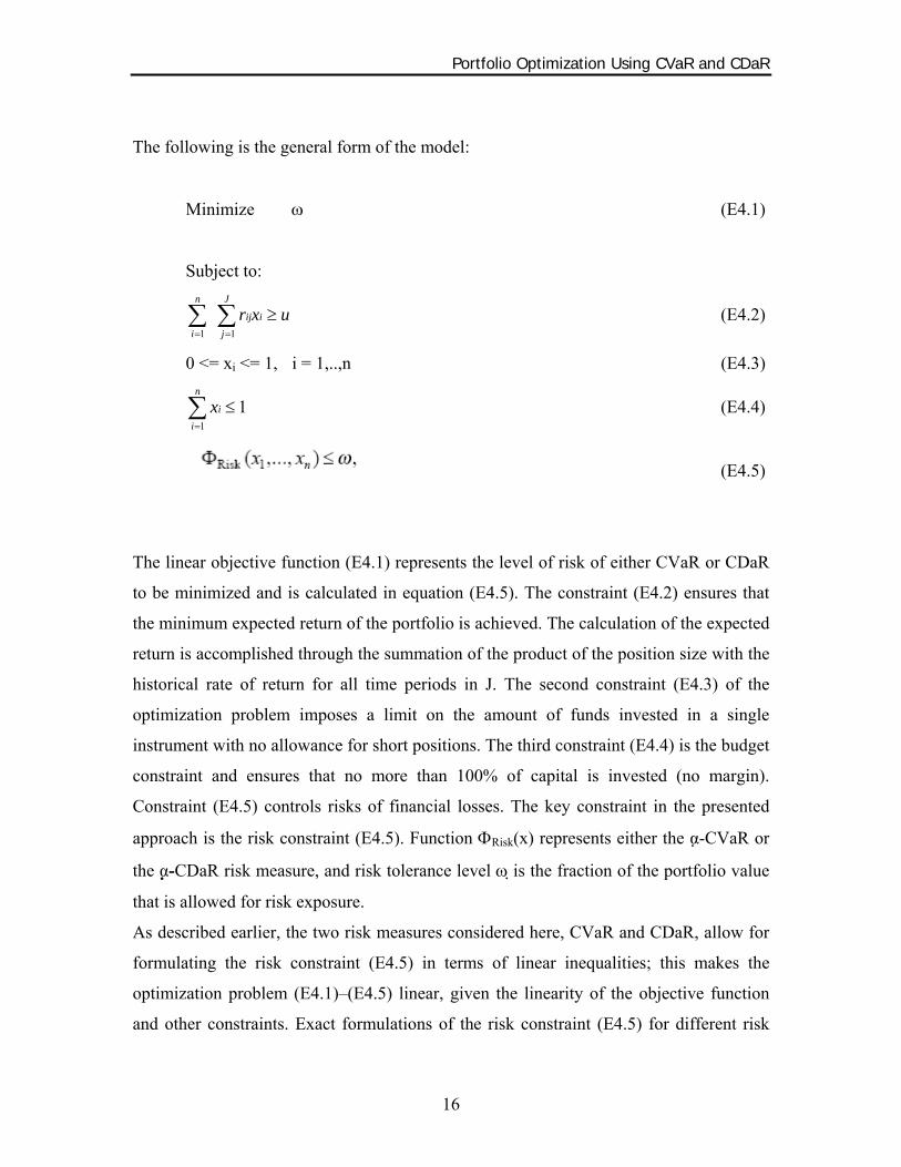
The following is the general form of the model:
Minimize ω (E4.1)
Subject to:
uxrJ
jiij
n
i≥∑∑
== 11 (E4.2)
0 <= xi <= 1, i = 1,..,n (E4.3)
11
≤∑=
n
iix (E4.4)
(E4.5)
The linear objective function (E4.1) represents the level of risk of either CVaR or CDaR
to be minimized and is calculated in equation (E4.5). The constraint (E4.2) ensures that
the minimum expected return of the portfolio is achieved. The calculation of the expected
return is accomplished through the summation of the product of the position size with the
historical rate of return for all time periods in J. The second constraint (E4.3) of the
optimization problem imposes a limit on the amount of funds invested in a single
instrument with no allowance for short positions. The third constraint (E4.4) is the budget
constraint and ensures that no more than 100% of capital is invested (no margin).
Constraint (E4.5) controls risks of financial losses. The key constraint in the presented
approach is the risk constraint (E4.5). Function ΦRisk(x) represents either the α-CVaR or
the α -CDaR risk measure, and risk tolerance level ω is the fraction of the portfolio value
that is allowed for risk exposure.
As described earlier, the two risk measures considered here, CVaR and CDaR, allow for
formulating the risk constraint (E4.5) in terms of linear inequalities; this makes the
optimization problem (E4.1)–(E4.5) linear, given the linearity of the objective function
and other constraints. Exact formulations of the risk constraint (E4.5) for different risk

Portfolio Optimization Using CVaR and CDaR
17
functions can be found in the following sections. Both risk measures are equally
important in this project; however the formulation of CVaR taken from [4] will be of
particular importance since it will be used to help derive the linear formulation of CDaR. 4.2 CVaR Risk Constraint Linear Transformation
The reduction of the CVaR risk management problem to a linear program is relatively
simple due to the possibility of replacing CVaR with some function which is convex and
piece-wise linear.
According to [4], the optimization problem with multiple CVaR constraints:
is equivalent to the following problem:
Then the risk constraint (E4.5), ΦRisk(x) ≤ ω, where the CVaR risk function replaces the
function ΦRisk(x), reads as:
(E4.6a)
where r ij is return asset i in time period j for j= 1,...,J. The loss function f(x,yj), defined as
the negative portfolio return at time j, is seen in the previous equation and is defined as:
(E4.6b)

Portfolio Optimization Using CVaR and CDaR
18
Since the loss function (E4.6b) is linear, and therefore convex, the risk constraint (E4.6a)
can be equivalently represented by the following set of linear inequalities according to
[4]:
(E4.7)
(E4.8)
(E4.9)
This representation allows for reducing the optimization problem (E4.1)–(E4.5) with the
CVaR constraint to a linear programming problem.
4.3 CDaR Risk Constraint Linear Transformation
Let rij be the rate of return of asset i in trading period j (this corresponds to j-th year in
this project), for j= 1,...,J. Assume the initial portfolio value equals 1. Let xi , i= 1,...,n be
the position size of assets in the portfolio. The uncompounded portfolio value at time j
equals [4]:
(E4.10)
The drawdown function f(x,rj) at time j is defined as the drop in the portfolio
value compared to the maximum value achieved before the time moment j [4]:
(E4.11)
The CDaR risk constraint ΦRisk(x)≤ ω has the form:

Portfolio Optimization Using CVaR and CDaR
19
(E4.12)
According to [4], (E4.12) can be reduced to a set of linear constraints in a similar method
to the CVaR constraint. This method was presented in the previous section. The
following set of constraints represents the first step in the reduction process:
,11
11
ωα
ζ ≤−
+ ∑=
J
jjw
J (E4.13)
(E4.14)
Where the portfolio high water mark (the highest value of the portfolio up to time j) is:
(E4.15)
The portfolio high water mark can be modeled linearly through the use of two
constraints:
(E4.16)
(E4.17)
Where (E4.16) ensures that each point uk for k = 1,..,J, is at least greater than or equal to
the portfolio value at time k and (E4.17) ensures that uk for k = 1,..,J, is at least greater
than or equal to the value of all previous points in the portfolio’s entire series.
This reduces equation (E4.14) to the following:
(E4.18)
,max,0max11
11 11 111
ωζα
ζ ≤⎥⎥⎦
⎤
⎢⎢⎣
⎡−⎥
⎦
⎤⎢⎣
⎡−⎥
⎦
⎤⎢⎣
⎡⎥⎦
⎤⎢⎣
⎡−
+ ∑ ∑∑ ∑∑= == =≤≤=
n
i
j
s
n
i
k
sjk
J
jiisis xrxir
J
,max1 11 11
j
n
i
j
s
n
ii
k
sjkwxrxr iisis ≤−⎥
⎦
⎤⎢⎣
⎡−⎥
⎦
⎤⎢⎣
⎡⎥⎦
⎤⎢⎣
⎡ ∑ ∑∑ ∑= == =
≤≤ζ
⎥⎦
⎤⎢⎣
⎡⎥⎦
⎤⎢⎣
⎡∑ ∑= =
≤≤
n
i
k
sjkiis xr
1 11max
,1 1
k
n
i
k
suxr iis ≤⎥
⎦
⎤⎢⎣
⎡⎥⎦
⎤⎢⎣
⎡∑ ∑= =
kk uu ≤− 1
,1 1
j
n
i
j
s
j wxru iis ≤−⎥⎦
⎤⎢⎣
⎡− ∑ ∑
= =
ζ

Portfolio Optimization Using CVaR and CDaR
20
(E4.19)
Where the portfolio value at time j is:
∑ ∑= =
⎥⎦
⎤⎢⎣
⎡n
i
j
siis xr
1 1
(E4.20)
Putting the entire set of equations together, the CDaR risk constraint ΦRisk(x) ≤ ω (E4.5)
can be replaced by the following set of equations:
(E4.13)
j = 1,..,J (E4.18)
k=1,..,J (E4.16)
(E4.17)
,R∈ζ (E4.21)
Jjwj ,....,1,0 =≥ (E4.19) Equation (E4.21) was added to ensure that ζ is an element of the set of real numbers. The
ζ variable represents the threshold value that is exceeded by (1-α)*J drawdowns. It
ensures that the correct amount of worst case drawdowns is optimized and that all other
drawdowns are left out of the series that is used for optimization.
It should be noted that for values of α that approach 1, the above CDaR constraint
becomes maximum drawdown, and for values of α that approach 0, the above CDaR
constraint becomes the average drawdown in the drawdown series. This also applies for
,0 jw≤
,1 1
j
n
i
j
sj wxru iis ≤−⎥
⎦
⎤⎢⎣
⎡− ∑ ∑
= =
ζ
,1 1
k
n
i
k
suxr iis ≤⎥
⎦
⎤⎢⎣
⎡⎥⎦
⎤⎢⎣
⎡∑ ∑= =
Jkuu kk
,....,11
=≤−
ωα
ζ ≤−
+ ∑=
J
jjw
J 1
11
1

Portfolio Optimization Using CVaR and CDaR
21
the set of equations for CVaR (E4.7) – (E4.9), where values of α that approach 1, the
CVaR constraint becomes maximum loss, and for values of α that approach 0, the CVaR
constraint becomes the average loss.
4.4 Data Selection
The next step involved gathering historical data for a set of assets to test the portfolio risk
optimization model. The Goldman Sachs Commodity Index 5 sub-indices yearly returns
from 1986-1995 were chosen for the testing. The next problem was deciding how the
data would be formatted.
4.4.1 Data Format
One assumption that is required in the formulated model presented earlier in section 4.1
is that the rate of return data used in the model has to be logarithmic. In order to
demonstrate this necessity, a comparison of geometric vs. logarithmic returns follows.
There are two methods of modeling returns in finance: geometric and
logarithmic/continuously compounded returns. The following figure from [5] gives an
overview of geometric and logarithmic returns for single and multi periods. Pt and Pt+1
denote the absolute asset value at time points t and t+1 respectively.
Figure 3: Geometric vs. Logarithmic Single and Multi-period Returns [5]
With geometric returns, the calculation is relative to previous periods’ returns and cannot
be used in an additive sense which is a requirement for the linear program. With the
continuously compounded returns, however, the change gets calculated on an
infinitesimally small time period and, as a result, the logarithmic return represents the
actual value at every time point. The logarithmic return can also be used additively for
the linear program. Adding up the rates of change over multiple periods will come to a
cumulative continuously compounded rate of change; therefore, logarithmic returns are

Portfolio Optimization Using CVaR and CDaR
22
required as model inputs. This requires any returns given in geometric format to be
converted into logarithmic returns.
4.4.2 Historical Data Sources
It has already been established that logarithmic returns are required for the model. This is
not a problem, however, because a series of asset values can be converted into a
logarithmic return series quite easily with the formulae in Figure 3 seen in the previous
section.
The dataset for the numerical experiments was provided by the Van Eck Associates
Corporation. It consisted of the annual returns of the Goldman Sachs Commodity Index
sub-indices from 1986-1995. The sub-indices of the broad index that were used in this
project are:
• Agriculture
• Energy
• Industrial Metals
• Livestock
• Precious Metals
This historical data was used as direct input into the model. The data can be seen in
geometric and logarithmic form in Appendix A.
4.5 Computer Model Programming
Various computer software packages can be used to solve the portfolio optimization
model formulated in Sections 4.1-4.3. The model was coded for use in the ILOG OPL
Development Studio IDE which utilizes CPLEX. The code itself was developed entirely
through testing and utilization of samples of other generic code.
The code can be seen in entirety in Appendix B and the mapping of the code to the
formulated model is included in Appendix C. The code is divided into two files. The first
file contains the variables, the objective function and the constraints. The second file
contains the data for the variables. When testing the model, two sections of the code were
being changed: the objective function and the expected return.
The first is the objective function seen below.
Portfolio Optimization Using CVaR and CDaR
23
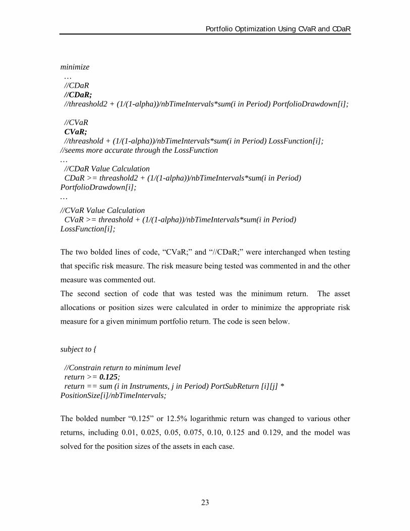
minimize … //CDaR //CDaR; //threashold2 + (1/(1-alpha))/nbTimeIntervals*sum(i in Period) PortfolioDrawdown[i]; //CVaR CVaR; //threashold + (1/(1-alpha))/nbTimeIntervals*sum(i in Period) LossFunction[i]; //seems more accurate through the LossFunction … //CDaR Value Calculation CDaR >= threashold2 + (1/(1-alpha))/nbTimeIntervals*sum(i in Period) PortfolioDrawdown[i]; …
//CVaR Value Calculation CVaR >= threashold + (1/(1-alpha))/nbTimeIntervals*sum(i in Period) LossFunction[i];
The two bolded lines of code, “CVaR;” and “//CDaR;” were interchanged when testing
that specific risk measure. The risk measure being tested was commented in and the other
measure was commented out.
The second section of code that was tested was the minimum return. The asset
allocations or position sizes were calculated in order to minimize the appropriate risk
measure for a given minimum portfolio return. The code is seen below.
subject to { //Constrain return to minimum level return >= 0.125; return == sum (i in Instruments, j in Period) PortSubReturn [i][j] * PositionSize[i]/nbTimeIntervals;
The bolded number “0.125” or 12.5% logarithmic return was changed to various other
returns, including 0.01, 0.025, 0.05, 0.075, 0.10, 0.125 and 0.129, and the model was
solved for the position sizes of the assets in each case.

Portfolio Optimization Using CVaR and CDaR
24
5. ANALYSIS OF RESULTS 5.1 Asset Analysis
Prior to running the optimization trials, a statistical analysis of the asset data was
performed. The result of a correlation and covariance analysis between the chosen assets
is shown in Tables 2 and 3. This analysis was performed using Microsoft excel and
illustrates the relationships between the asset returns. The Precious Metals and
Agriculture assets have the least in common with all other assets and are therefore likely
to provide some diversification in the optimization of risk.
Industrial
Metals Precious Metals Energy Agriculture Livestock
Industrial Metals 1 Precious Metals 0.135571 1 Energy 0.350152 -0.0046 1 Agriculture 0.246102 0.066101 0.142745 1 Livestock 0.50327 0.092125 0.418922 0.132691 1
Table 2: Correlation between Assets
Industrial
Metals Precious Metals Energy Agriculture Livestock
Industrial Metals 0.088375 Precious Metals 0.00444 0.012135 Energy 0.038876 -0.00019 0.139485 Agriculture 0.011339 0.001129 0.008262 0.02402 Livestock 0.023385 0.001586 0.024455 0.003214 0.024431
Table 3: Covariance between Assets
Table 4 has the total annualized and cumulative returns for all of the assets used in
testing.

Portfolio Optimization Using CVaR and CDaR
25
Industrial
Metals Precious Metals Energy Agriculture Livestock
Cumulative Return 258% 63% 244% -1% 150% Annualized Return 12.91% 3.17% 12.20% -0.07% 7.52%
Table 4: Asset Returns
5.2 Portfolio Results – Efficient Frontier & Portfolio Analysis
The portfolio optimization model described in sections 4.2-4.4 with equations (E4.1) to
(E4.5) was run to obtain a specific expected return and minimize a given risk measure.
This procedure was repeated several times to get a series of CVaR and CDaR values (as a
percentage of portfolio risk) versus the expected return obtained. In order to determine
the range of expected returns for the portfolio parameter, the returns of the individual
assets had to be investigated. The range of expected returns is defined as the interval
between the smallest and the largest expected return of the individual assets. This is due
to the assumption that under the circumstances of no borrowing and no short sales, it is
not possible to reach an expected portfolio return that is outside this interval. As seen in
Table 4, the highest annual return was the Industrial Metals asset with a return of 12.91%
and the lowest annual return was with the Agriculture asset with -0.07%.
The alpha parameter for the α-CVaR and α-CDaR optimization is chosen as 0.80. With
an alpha parameter of 0.80, the risk functions will take into consideration the worst 20%
(1-0.80) of portfolio losses or drawdowns. The result is shown in the efficient frontier
graph in Figure 4, where the portfolio rate of return is the yearly rate of return.

Portfolio Optimization Using CVaR and CDaR
26
Efficient Frontier: 0.8 - CVaR and 0.8 - CDaR
0%
2%
4%
6%
8%
10%
12%
14%
0% 5% 10% 15% 20% 25% 30% 35%
Risk %
Retu
rn %
(yea
rly)
0.8 - CVaR0.8 - CDaR
Figure 4: Efficient Frontier for 0.8-CVaR and 0.8-CDaR Portfolios
After some testing it was decided to raise the minimum end of the range of expected
returns due to the convergence of the asset allocation entirely to one asset, resulting in a
major increase in portfolio risk as reflected by both 0.8-CVaR and 0.8-CDaR. The
minimum was raised to 1%.
The efficient frontiers rightfully converge to the point of maximum return (12.91%) at
different levels of risk. The 0.8-CVaR measure converges at 18.49%, while 0.8-CDaR
converges at a greater risk level of 29.84%. This confirmed the hypothesis that CDaR is a
more conservative risk measure, and would therefore converge at a greater risk level than
the CVaR risk measure. This can be explained by the fact that CDaR takes into
consideration losses and their sequence, while CVaR only takes into consideration single
period losses.
The efficient frontier of the 0.8-CDaR optimization is much more unstable than that of
0.8-CVaR. This can be seen in Figure 4 where the 0.8-CDaR efficient frontier graph
shows that the risk is constant for several points of return, up to a return of 7.82%. For all
other returns under 7.82% the risk level (as defined by 0.8-CDaR) would actually
increase if the minimum return constraint was an equality.

Portfolio Optimization Using CVaR and CDaR
27
The instability is the effect of several factors. Firstly, the data set being used is small and
consists of 20 points per asset. This combined with the fact that 0.8-CDaR takes only the
worst case (20% in our optimization with alpha set to 0.80) drawdowns into consideration
means that the 0.8-CDaR value series is limited. For example, in this series of 20 points,
10 were drawdowns from the peak, so 20% of worst case drawdowns would be 2 data
points. The algorithm is optimizing the value of these two data points, contributing to the
effect observed on the efficient frontier. Secondly, the dataset used was the yearly
commodity returns over a 20 year period. Commodity prices are known to be extremely
volatile in nature, especially when returns are looked at over the period of an entire year.
Thirdly, α-CDaR is sensitive not only to the magnitude of portfolio losses but also to
their sequence. This makes the risk measure more sensitive in general. These three
factors contributed greatly to the effect seen on the efficient frontier. In theory, the effect
would be minimized or disappear as soon as the amount of data increased and/or a less
volatile dataset was introduced. The 0.8-CVaR efficient frontier graph also shows a small
period (up to 2.51% return) where the risk is constant for several points of return, but it is
far less substantial than the effect seen with the 0.8-CDaR measure.
Figures 5 and 6 show the 0.8-CVaR and 0.8-CDaR portfolio value series for two different
risk levels. Increased portfolio value fluctuations can be seen in the higher risk series.

Portfolio Optimization Using CVaR and CDaR
28
0.8 - CVaR Portfolio
0
0.5
1
1.5
2
2.5
3
3.5
4
0 5 10 15 20
Year (0 = Start)
Por
tofo
lio V
alue
(1 =
Sta
rt)
9.23% CVaR18.49% CVaR
Figure 5: 0.8-CVaR Portfolio Value Series
0.8 - CDaR Portfolio
0
0.5
1
1.5
2
2.5
3
3.5
4
0 5 10 15 20
Year (0 = Start)
Portf
olio
Val
ue (1
= S
tart
)
18% CDaR25% CDaR
Figure 6: 0.8-CDaR Portfolio Value Series
A detailed breakdown of portfolio losses in the 0.8-CVaR portfolio can be seen in Figure
7. The difference between the two portfolio risk profiles is very evident. The 18.49% 0.8-

Portfolio Optimization Using CVaR and CDaR
29
CVaR portfolio exhibits multiple losses exceeding the greatest loss of the 9.23% 0.8-
CVaR portfolio. It is also observed that even though the 9.23% 0.8-CVaR portfolio
optimizes the worst 20% of losses, in this trial it has the effect of significantly reducing
the magnitude of the remaining 80% of losses and, therefore, the overall risk. This
phenomenon could be a dataset specific event.
0.8 - CVaR Portfolio Loss Series
0%
5%
10%
15%
20%
25%
- 5 10 15 20
Year (0 = Start)
Loss
(%)
9.23% CVaR Loss 18.49% CVaR Loss
Figure 7: 0.8-CVaR Portfolio Loss Series
A detailed breakdown of portfolio drawdowns in the 0.8-CDaR portfolio is shown in
Figure 8. One major difference between the drawdown series seen in Figure 8 and the
loss series seen in Figure 7 is that the drawdowns build in magnitude over time, whereas
the losses are single events. This is to be expected due to the characteristic of the
drawdown function to impose penalties based on not only on the magnitude of the losses
but also their sequence. Small consecutive losses can lead to a large drawdown without
significantly increasing the losses seen by CVaR.

Portfolio Optimization Using CVaR and CDaR
30
0.8 - CDaR Portfolio Drawdown Series
0%
5%
10%
15%
20%
25%
30%
35%
40%
0 5 10 15 20
Year (0 = Start)
Draw
dow
n (%
)
18% CDaR Drawdown 25% CDaR Portfolio
Figure 8: 0.8-CDaR Portfolio Drawdown Series
Both risk levels exhibit a similar pattern in portfolio drawdowns. The 25% 0.8-CDaR
portfolio shows greater extreme drawdown points than the 18% 0.8-CDaR. However, it is
interesting to note that the 18% 0.8-CDaR portfolio spends a very long interval in
drawdown starting in the 12th time period. It can be hypothesized that increasing the
percentage of drawdowns to be considered by the CDaR optimization from 20% to a
higher number would result in a much greater risk reading for the portfolio, whereas
doing the same for the 25% CDaR portfolio might not increase the risk read as
expediently.
5.3 Portfolio Results – Asset Allocation/ Position Sizing Analysis
The purpose of allocating different amounts of capital amongst different assets is to
benefit from the nature of certain assets to be uncorrelated or negatively correlated to
others at times. In this project the changing allocation or position size of the assets will
directly affect the portfolio risk as measured by the 0.8-CVaR and 0.8-CDaR.

Portfolio Optimization Using CVaR and CDaR
31
Figure 9 shows the asset allocation results for the 0.8-CVaR portfolio for a given level of
return while minimizing loss risk.
0.8 - CVaR Portfolio: Return vs. Asset Allocation
-20%
0%
20%
40%
60%
80%
100%
120%
0% 2% 4% 6% 8% 10% 12% 14%
Portoflio Return
% o
f Ass
et A
lloca
tion
Industrial Metals Precious Metals EnergyAgriculture Livestock
Figure 9: 0.8-CVaR Portfolio: Return vs. Asset Allocation
The results show the effect of diversification clearly: in the low end of the return
spectrum, Precious Metals and Agriculture receive the majority of the capital allocation.
The correlation coefficient between these assets is 0.066 indicating that they are two
uncorrelated assets and thus help to offset the portfolio risk. The allocation of capital to
Livestock begins to increase almost immediately. Livestock has a low correlation
coefficient to both Precious Metals and Agriculture, with a coefficient less than 0.15 for
both. Nearing the peak of the allocation of capital to Livestock, the Industrial Metals
asset begins to receive capital heavily. This is due to the highest possible return being in
the Industrial Metals asset but this return is not without a tradeoff in volatility. The
allocation continues until all the capital is positioned into the Industrial Metals asset.
Energy does not receive any capital throughout the entire allocation process.
Figure 10 illustrates the number of assets allocated versus the return and risk of the
portfolio. It is clear that throughout much of the return spectrum, the allocation of capital

Portfolio Optimization Using CVaR and CDaR
32
to several assets was used to offset portfolio risk as measured by 0.8-CVaR. Figure 10
quantifies this measure by showing the number of assets in which capital is allocated.
Three assets are allocated for all portfolio returns up to 10% at which point the allocation
decreases to two assets and finally converges to a single asset. This confirms the
assumption that the allocation will have to converge to one asset as the portfolio
approaches the maximum return limit. The comparison of the number of allocated assets
vs. portfolio risk also illustrates similar behavior, as capital is allocated into three assets
below a risk threshold of 12.42%. As portfolio risk increases to 17.5% the diversification
of capital is reduced to two assets and finally one asset at a risk measure of 18.5%.
0.8-CVaR Portfolio: Number of Allocated Assets Vs. Return
0
1
2
3
4
0% 2% 4% 6% 8% 10% 12% 14%
Return
Num
ber o
f Allo
cate
d As
sets
0.8-CVaR Portfolio: Number of Allocated Assets vs. Risk
0
1
2
3
4
7% 9% 11% 13% 15% 17% 19% 21%
Risk - 0.8-CVaR
Num
ber o
f Allo
cate
d A
sset
s
Figure 10: 0.8-CVaR Portfolio: Number of Asset Allocated vs. Return and Risk
Figure 11 demonstrates the asset allocation results for the 0.8-CVaR portfolio for a
specified level of risk. In line with the results depicted in Figure 10, the portfolio initially
contains three assets and transitions to two assets, finishing with all the capital allocated
into one asset at the portfolio return limit. The decreasing diversification occurs while
risk increases rapidly.

Portfolio Optimization Using CVaR and CDaR
33
0.8 - CVaR Portfolio: Risk vs. Asset Allocation
-20%
0%
20%
40%
60%
80%
100%
120%
7% 9% 11% 13% 15% 17% 19%
Portfolio Risk (0.8-CVaR)
% o
f Ass
et A
lloca
tion
Industrial Metals Precious Metals EnergyAgriculture Livestock
Figure 11: 0.8-CVaR Portfolio: Risk vs. Asset Allocation
Table 5 summarizes the data used in Figures 4, 9-11 and displays the results of the 0.8-
CVaR portfolio allocation at various rates of return and risk.
Portfolio Allocation by Return – 0.8 – CVaR
Return 0.8-
CVaR Industrial
Metals Precious
Metals Energy Agriculture Livestock
Number of Assets
Allocated 1.00% 8.44% 0.00% 73.14% 0.00% 21.52% 5.34% 3 2.50% 8.44% 0.00% 73.14% 0.00% 21.52% 5.34% 3 5.00% 9.23% 5.49% 60.92% 0.00% 0.00% 33.59% 3 7.50% 10.53% 12.75% 15.84% 0.00% 0.00% 71.42% 3 10.00% 12.42% 47.33% 2.34% 0.00% 0.00% 50.33% 3 12.50% 17.51% 91.55% 0.00% 0.00% 0.00% 8.45% 2 12.90% 18.38% 98.95% 0.00% 0.00% 0.00% 1.05% 2 12.96% 18.49% 100.00% 0.00% 0.00% 0.00% 0.00% 1
Table 5: 0.8-CVaR Portfolio Allocation Details
Figure 12 shows the asset allocation results for the 0.8-CDaR portfolio for a given level
of return while minimizing drawdown risk.

Portfolio Optimization Using CVaR and CDaR
34
0.8 - CDaR Portfolio: Return vs. Asset Allocation
-20%
0%
20%
40%
60%
80%
100%
120%
0% 5% 10% 15%
Portoflio Return
% o
f Ass
et A
lloca
tion
Industrial Metals Precious Metals EnergyAgriculture Livestock
Figure 12: 0.8-CDaR Portfolio: Return vs. Asset Allocation
The first thing that is evident from Figure 12 is the aforementioned problem with the 0.8-
CDaR measure where the portfolio assets are allocated in the same fashion below a return
level of 7.82%. In the low end of the spectrum, four assets receive capital, with
Agriculture being the only asset not to receive any allocation throughout the entire
dataset. It is interesting to note that Energy received capital allocations in the 0.8-CDaR
trials but did not in the 0.8-CVaR trials. This could be due to the Energy data series
positively affecting not only the magnitude of losses but also their sequence, which
drawdowns take into consideration. A large allocation of capital is made to Precious
Metals once again for much of the return spectrum. This is likely the result of the asset
being largely uncorrelated to the others. Once again the portfolio converges on Industrial
Metals while all other asset allocations go to zero.

Portfolio Optimization Using CVaR and CDaR
35
0.8 - CDaR Portfolio: Number of Allocated Assets vs. Return
0
1
2
3
4
5
0% 2% 4% 6% 8% 10% 12% 14%
Return
Num
ber o
f Allo
cate
d A
sset
s
0.8 - CDaR Portfolio: Number of Allocated Assets vs. Risk
0
1
2
3
4
5
15% 20% 25% 30% 35% 40%
Risk - 0.8-CDaR
Num
ber o
f Allo
cate
d A
sset
s
Figure 13: 0.8-CDaR Portfolio: Number of Asset Allocated vs. Return and Risk
Figure 13 illustrates the number of assets allocated versus the return and risk of the
portfolio. This figure illustrates the same conclusions as seen previously in Figure 10 for
the 0.8-CVaR portfolio. One important difference is that capital is allocated to a
maximum of 4 of the portfolio assets in this case, whereas only a maximum of 3 was
achieved with 0.8-CVaR. This is likely due to the fact that drawdowns take into
consideration loss sequence and magnitude, and therefore 4 assets will increasingly
diversify the portfolio during lengthy drawdown scenarios.
0.8 - CDaR Portfolio: Risk vs. Asset Allocation
-20%
0%
20%
40%
60%
80%
100%
120%
15% 20% 25% 30%
Portfolio Risk (CDaR)
% o
f Ass
et A
lloca
tion
Industrial Metals Precious Metals EnergyAgriculture Livestock
Figure 14: 0.8-CDaR Portfolio: Risk vs. Asset Allocation

Portfolio Optimization Using CVaR and CDaR
36
Figure 14 demonstrates the asset allocation results for the 0.8-CDaR portfolio for a
specified level of risk. The portfolio starts off with relatively higher risk levels in
comparison to 0.8-CVaR. This allows much of the portfolio to be positioned into
Industrial Metals, a risky but high reward asset. As the portfolio risk increases the
allocation to this asset is increased even further, and the allocation to other assets
diminishes along with portfolio diversification.
Table 6 summarizes the data used in Figures 4, 12-14 and displays the results of the 0.8-
CDaR portfolio allocation at various rates of return and risk.
Portfolio Allocation - 0.8-CDaR Portfolio
Return 0.8-
CDaR Industrial
Metals Precious Metals Energy Agriculture Livestock
Number of Assets
Allocated 1.00% 17.76% 35.76% 39.68% 3.97% 0.00% 20.59% 4 2.50% 17.76% 35.76% 39.68% 3.97% 0.00% 20.59% 4 5.00% 17.76% 35.76% 39.68% 3.97% 0.00% 20.59% 4 7.50% 17.76% 35.76% 39.68% 3.97% 0.00% 20.59% 4 10.00% 19.30% 54.14% 17.40% 7.07% 0.00% 21.39% 4 12.50% 25.31% 80.84% 0.00% 12.20% 0.00% 6.96% 3 12.90% 29.84% 91.41% 0.00% 8.59% 0.00% 0.00% 2 12.96% 34.97% 100.00% 0.00% 0.00% 0.00% 0.00% 1
Table 6: 0.8-CDaR Portfolio Allocation Details

Portfolio Optimization Using CVaR and CDaR
37
6. CONCLUSION This project analyzed the impacts of risk measures on the position sizing of a portfolio.
The Conditional Value-At-Risk and Conditional Drawdown-At-Risk risk measures were
utilized to optimally allocate the assets of a portfolio. The assets that were chosen are the
yearly returns of the give Goldman Sachs Commodity Indices.
A linear portfolio rebalancing algorithm was developed and used to optimize asset
allocation. Research on the CVaR and CDaR risk measures was performed to formulate
the risk measures linearly, thus allowing for use in a linear programming framework.
This framework was modeled in the ILOG OPL Development Studio IDE in order to
analyze the effectiveness of using risk measures to determine asset allocation. Several
portfolio allocations were created through the optimization of risk for both risk measures,
CDaR and CVaR, while ensuring that the portfolio return was constrained to a minimum
level. An analysis of the results of the allocation followed, including the construction of
efficient frontiers, sample portfolio series, CVaR loss functions, CDaR drawdown
functions, and detailed portfolio allocation graphs for both series as well as the
quantification of portfolio asset allocation in relation to return and risk.
The CDaR risk measure was seen to be less reliable than the CVaR risk measure as
illustrated in the efficient frontier in Figure 4. This was attributed to three factors: firstly,
the dataset only consisted of 20 periods per asset with 5 assets, which limited the amount
of drawdown data the algorithm takes into consideration. Secondly, the dataset was
composed of yearly data that was highly volatile, restricting the amount of risk that could
be eliminated. Thirdly, CDaR is sensitive not only to the magnitude of portfolio losses
but also to their sequence. The effects of these three factors are explained in greater detail
in section 5.2.
It was determined that CDaR is a more conservative measure of risk than CVaR. This
can be seen in the efficient frontier shown in Figure 4, and can be attributed to the fact
that for a given percentage of return, CDaR has a greater level of risk than CVaR. CDaR
is more conservative in nature as it considers both the magnitude as well as the sequence
of losses, whereas only the magnitude of losses is a factor for CVaR.

Portfolio Optimization Using CVaR and CDaR
38
Several trends were observed related to asset diversification. For both CVaR and CDaR,
portfolio risk was shown to increase with an allocation of capital to less assets. Therefore,
risk increased with decreasing asset diversification. As well, the return increased as less
assets were utilized in the portfolio and risk increased.
Capital was allocated to assets with lower correlations to offset risk. For the CVaR risk
measure, assets with lower correlations tended to dominate asset allocation for the low
end of the risk spectrum. CDaR demonstrated the same result with a large allocation to
Precious Metals in the low risk spectrum. The Precious Metals asset is the least correlated
to all other assets, and, therefore, is utilized in reducing portfolio risk.
In order to gain a deeper understanding of these risk measures, it is recommended that
further research be conducted. The following section explores research ideas.

Portfolio Optimization Using CVaR and CDaR
39
7. FURTHER RESEARCH
There are several additional research paths that can be taken to further refine and expand
on the financial optimization model and risk measures presented in this project.
The first recommendation is the investigation of the reliability of the CDaR risk measure.
The efficient frontier for CDaR was constant for levels of return under 7.82%. This
behavior could be analyzed by utilizing a larger dataset that includes assets that are more
highly uncorrelated or negatively correlated and less volatile. Additionally, an adjustment
should be made in the alpha parameter of the risk measures, and the effect of increasing
and decreasing the fraction of drawdowns or losses that the risk measure takes into
consideration should be explored.
Secondly, further work should attempt to explore the effect of changing the constraints
that affect how much capital can be allocated to the assets. Methods such as short selling
and using limited amounts of margin to buy assets could be explored.
Finally, whereas the testing done in this project delves mainly into looking at the efficient
frontiers and optimal portfolio structure for the risk measures and expected returns, it
does not demonstrate the performance of the approach in an investment environment. An
investment environment should be simulated with historical data. The test should begin
with performing a portfolio rebalancing according to the maximization of reward to risk
measures and on a predetermined set of data points from the beginning of the data set.
The future data points in the series would be treated as realized data points in the future
of the portfolio. The portfolio should then be rebalanced after every additional data point
in the series. The rebalancing of the data could be performed in two ways: using the
entire data series from start to finish or using a rolling window of a determined length.
This research would look further into the practical applications of using these risk
algorithms for active portfolio management.
Portfolio Optimization Using CVaR and CDaR
40
8. REFERENCES
[1] J. Schwager, Market Wizards. HarperCollins, 1993. [2] Van K. Tharp, “Special Report on Money Management” I.I.T.M., Inc., 1997. [3] J. Ginyard, “Position-sizing Effects on Trader Performance: An experimental
analysis” Masters Thesis, University/Stockholm School of Economics, Stockholm, Sweden, 2001.
[4] P. A. Krokhmal, S. P. Uryasev and G. M. Zrazhevsky, "Comparative Analysis of
Linear Portfolio Rebalancing Strategies: An Application to Hedge Funds". U of Florida ISE Research Report No. 2001-11, November, 2001. Available at SSRN: http://ssrn.com/abstract=297639 or DOI: 10.2139/ssrn.297639
[5] S. Johri, “PORTFOLIO OPTIMIZATION WITH HEDGE FUNDS: Conditional
Value At Risk And Conditional Draw-Down At Risk For Portfolio Optimization With Alternative Investments” Masters Thesis, Department of Computer Science of Swiss Federal Institute of Technology, Zurich, 2004.
[6] S. Benninga and Z. Wiener, “Value-at-Risk (VaR)” Mathematica in Education
and Research, Vol. 7 No.4, 1998.
[7] S. P. Uryasev, “Conditional Value-at-Risk: Optimization Algorithms and Applications”. Financial Engineering News, February, 2000. Available at: http://www.fenews.com/fen14/valueatrisk.html
[8] R. T. Rockafellar and S. Uryasev, “Optimization of Conditional Value-at-Risk” U of Florida ISE Research Report, Florida, USA, September, 1999.
[9] R. T. Rockafellar and S. P. Uryasev, "Conditional Value-at-Risk for General Loss
Distributions" EFA 2001 Barcelona Meetings, EFMA 2001 Lugano Meetings; U of Florida, ISE Dept. Working Paper No. 2001-5, April 4, 2001. Available at SSRN: http://ssrn.com/abstract=267256 or DOI: 10.2139/ssrn.267256
[10] A. Chekhlov, S. P. Uryasev and M. Zabarankin, "Portfolio Optimization with
Drawdown Constraints" Research Report #2000-5, April 8, 2000. Available at SSRN: http://ssrn.com/abstract=223323 or DOI: 10.2139/ssrn.223323
[11] A. Chekhlov, S. P. Uryasev and M. Zabarankin, "Drawdown Measure in Portfolio
Optimization" June 25, 2003. Available at SSRN: http://ssrn.com/abstract=544742

Portfolio Optimization Using CVaR and CDaR
41
APPENDIX A
Historical Asset Return Data

Portfolio Optimization Using CVaR and CDaR
42
Historical Asset Return Data (Geometric Single Period Returns)
Industrial
Metals Precious Metals Energy Agriculture Livestock
1986 -3.1% 21.8% -22.0% -2.4% 22.5% 1987 153.9% 17.8% 13.3% 15.3% 47.0% 1988 78.6% -12.4% 32.3% 28.9% 23.2% 1989 0.1% -1.4% 84.9% -2.9% 15.6% 1990 45.6% -5.4% 45.3% -11.4% 26.6% 1991 -17.1% -10.8% -12.8% 13.1% 0.2% 1992 6.0% -4.3% 1.0% -8.5% 26.1% 1993 -16.0% 19.6% -33.7% 19.6% 7.8% 1994 65.1% -1.2% 7.5% 8.3% -11.3% 1995 -6.6% 2.0% 28.2% 27.0% 3.3% 1996 -8.8% -4.0% 66.0% -2.1% 15.2% 1997 -2.6% -14.0% -23.1% 4.7% -6.2% 1998 -19.2% -0.7% -46.8% -24.4% -27.6% 1999 30.7% 3.9% 92.4% -18.9% 14.4% 2000 -4.3% -1.2% 87.5% -1.1% 8.6% 2001 -16.5% 0.5% -40.4% -23.1% -2.9% 2002 -0.6% 23.3% 50.7% 11.4% -9.5% 2003 40.0% 16.3% 24.6% 6.6% 0.0% 2004 27.5% 8.6% 26.1% -20.2% 25.5% 2005 36.3% 18.6% 31.2% 2.4% 3.5%

Portfolio Optimization Using CVaR and CDaR
43
Historical Asset Return Data (Logarithmic Single Period Returns)
Industrial
Metals Precious Metals Energy Agriculture Livestock
1986 -3.1% 19.7% -24.8% -2.4% 20.3% 1987 93.2% 16.4% 12.5% 14.2% 38.5% 1988 58.0% -13.2% 28.0% 25.4% 20.9% 1989 0.1% -1.4% 61.5% -2.9% 14.5% 1990 37.6% -5.6% 37.4% -12.1% 23.6% 1991 -18.8% -11.4% -13.7% 12.3% 0.2% 1992 5.8% -4.4% 1.0% -8.9% 23.2% 1993 -17.4% 17.9% -41.1% 17.9% 7.5% 1994 50.1% -1.2% 7.2% 8.0% -12.0% 1995 -6.8% 2.0% 24.8% 23.9% 3.2% 1996 -9.2% -4.1% 50.7% -2.1% 14.1% 1997 -2.6% -15.1% -26.3% 4.6% -6.4% 1998 -21.3% -0.7% -63.1% -28.0% -32.3% 1999 26.8% 3.8% 65.4% -20.9% 13.5% 2000 -4.4% -1.2% 62.9% -1.1% 8.3% 2001 -18.0% 0.5% -51.8% -26.3% -2.9% 2002 -0.6% 20.9% 41.0% 10.8% -10.0% 2003 33.6% 15.1% 22.0% 6.4% 0.0% 2004 24.3% 8.3% 23.2% -22.6% 22.7% 2005 31.0% 17.1% 27.2% 2.4% 3.4%

Portfolio Optimization Using CVaR and CDaR
44
APPENDIX B
OPL Computer Code

Portfolio Optimization Using CVaR and CDaR
45
File: Thesis1-mod.mod /********************************************* * OPL 4.0 Model * Author: kuutane * Creation Date: Sat Jan 27 12:23:48 2007 *********************************************/ //variables int nbInstruments = ...; int nbTimeIntervals = ...; float alpha = 0.8; //alpha 0 = average 1 = maxloss range Instruments = 1..nbInstruments; range Period = 0..nbTimeIntervals; dvar float PositionSize[Instruments]; //size of position in investment (Fraction) dvar float PortfolioHighWaterMark[Period]; //Highest value the portfolio achieves up to <TimeIntevals> dvar float PortfolioDrawdown[Period]; //Difference between HWM and Current Portfolio Value dvar float LossFunction[Period]; //loss function for CVaR //dvar float aLossFunction[Period]; //test loss function for CVaR dvar float threashold; //threashhold CVaR - ensures only 20% of worst case losses are used for minimization calculation dvar float threashold2; //threashhold CDaR - ensures only 20% of worst case drawdowns are used for minimization calculation dvar float return; //portfolio return constraint dvar float CDaR; //CDaR value dvar float CVaR; //CVaR value // [ [0,1,2,3,4], [0,1,2,3,4],[0,1,2,3,4] ] float PortSubReturn [Instruments] [Period] = ...; //; //returns by period minimize //return – for maximization tests //sum (i in Instruments, j in Period) PortSubReturn [i][j] * PositionSize[i]/nbTimeIntervals; //CDaR //CDaR; //threashold2 + (1/(1-alpha))/nbTimeIntervals*sum(i in Period) PortfolioDrawdown[i];

Portfolio Optimization Using CVaR and CDaR
46
//CVaR CVaR; //threashold + (1/(1-alpha))/nbTimeIntervals*sum(i in Period) LossFunction[i]; //seems more accurate through the LossFunction subject to { //Constrain return to minimum level return >= 0.125; return == sum (i in Instruments, j in Period) PortSubReturn [i][j] * PositionSize[i]/nbTimeIntervals; //CDaR Value Calculation CDaR >= threashold2 + (1/(1-alpha))/nbTimeIntervals*sum(i in Period) PortfolioDrawdown[i]; //Portfolio High Water Mark Calculation forall(k in 0..nbTimeIntervals) PortfolioHighWaterMark[k] >= sum(i in Instruments,j in 0..k) PortSubReturn[i][j]*PositionSize[i]; //HWM[k] is greater InvestmentReturn[i][k]*PositionSize[i] for all i, k - current interval forall(k in 1..nbTimeIntervals) PortfolioHighWaterMark[k] >= PortfolioHighWaterMark[k-1]; //HWM[k] >= HWM[k-1] //Portfolio Drawdown Calculation forall(k in 1..nbTimeIntervals) PortfolioDrawdown[k] >= PortfolioHighWaterMark[k] - sum(i in Instruments,j in 0..k) PortSubReturn[i][j]*PositionSize[i] - threashold2; //PortfolioDrawdown[k] >= PortfolioHighWaterMark[k] - sum(i in Instruments) InvestmentReturn[i][k]*PositionSize[i] - threashold; forall(k in 0..nbTimeIntervals) PortfolioDrawdown[k] >= 0; //CVaR Value Calculation CVaR >= threashold + (1/(1-alpha))/nbTimeIntervals*sum(i in Period) LossFunction[i]; //Portfolio Loss Function Calculation forall(k in 0..nbTimeIntervals) LossFunction[k] >= - sum(i in Instruments) PortSubReturn[i][k]*PositionSize[i] - threashold;

Portfolio Optimization Using CVaR and CDaR
47
forall(k in 0..nbTimeIntervals) LossFunction[k] >= 0; /* //Test Loss Function Calculation forall(k in 0..nbTimeIntervals) aLossFunction[k] >= - sum(i in Instruments) PortSubReturn[i][k]*PositionSize[i]; forall(k in 0..nbTimeIntervals) aLossFunction[k] >= 0; */ //Standard Constraints forall (i in Instruments) PositionSize[i] >= 0; //no negative (short) positions forall (i in Instruments) PositionSize[i] <= 1; //no leveraged positions sum (i in Instruments) PositionSize[i] == 1; //Maximum Total Investment is 100%, no leverage } File: Thesis1-dat.dat nbInstruments = 5; //Number of Assets nbTimeIntervals = 20; //Number of Time Intervals // 5 asset series PortSubReturn = [[0 -0.0314,0.931,0.579,0.001,0.375,-0.18,0.05826,-0.17,0.501,-0.0682,-0.0921,-0.0263,-0.21,0.267,-0.0439,-0.18,-0.00601,0.336,0.242,0.309],[0 0.197,0.163,-0.13,-0.0140,-0.0555,-0.11,-0.0439,0.178,-0.0120,0.0198,-0.0408,-0.15,-0.0702,0.03825,-0.0120,0.004987,0.209,0.151,0.0825,0.170],[0 -0.24,0.124,0.279,0.614,0.373,-0.13,0.009950,-0.41,0.07232,0.248,0.506,-0.26,-0.63,0.654,0.628,-0.51,0.410,0.219,0.231,0.271],[0 -0.0242,0.142,0.253,-0.0294,-0.12,0.123,-0.0888,0.178,0.07973,0.239,-0.0212,0.04592,-0.27,-0.20,-0.0110,-0.26,0.107,0.06391,-0.22,0.02371],[0 0.202,0.385,0.208,0.144,0.235,0.001998,0.231,0.0751,-0.11,0.03246,0.141,-0.0640,-0.32,0.134,0.0825,-0.0294,-0.0998,0,0.227,0.0344]]; //Other test series // 3 asset series

Portfolio Optimization Using CVaR and CDaR
48
//PortSubReturn = [[0 0.197,0.163,-0.13,-0.0140,-0.0555,-0.11,-0.0439,0.178,-0.0120,0.0198,-0.0408,-0.15,-0.0702,0.03825,-0.0120,0.004987,0.209,0.151,0.0825,0.170],[0 -0.24,0.124,0.279,0.614,0.373,-0.13,0.009950,-0.41,0.07232,0.248,0.506,-0.26,-0.63,0.654,0.628,-0.51,0.410,0.219,0.231,0.271],[0 -0.0242,0.142,0.253,-0.0294,-0.12,0.123,-0.0888,0.178,0.07973,0.239,-0.0212,0.04592,-0.27,-0.20,-0.0110,-0.26,0.107,0.06391,-0.22,0.02371]]; // 2 asset series //PortSubReturn = [[0 0.197,0.163,-0.13,-0.0140,-0.0555,-0.11,-0.0439,0.178,-0.0120,0.0198,-0.0408,-0.15,-0.0702,0.03825,-0.0120,0.004987,0.209,0.151,0.0825,0.170],[0 -0.24,0.124,0.279,0.614,0.373,-0.13,0.009950,-0.41,0.07232,0.248,0.506,-0.26,-0.63,0.654,0.628,-0.51,0.410,0.219,0.231,0.271]];

Portfolio Optimization Using CVaR and CDaR
49
APPENDIX C
OPL Computer Code to Model Mapping

Portfolio Optimization Using CVaR and CDaR
50
minimize //return – for maximization tests //sum (i in Instruments, j in Period) PortSubReturn [i][j] * PositionSize[i]/nbTimeIntervals; //CDaR //CDaR; //threashold2 + (1/(1-alpha))/nbTimeIntervals*sum(i in Period) PortfolioDrawdown[i]; //CVaR CVaR; //threashold + (1/(1-alpha))/nbTimeIntervals*sum(i in Period) LossFunction[i]; //seems more accurate through the LossFunction subject to { //Constrain return to minimum level return >= 0.125; return == sum (i in Instruments, j in Period) PortSubReturn [i][j] * PositionSize[i]/nbTimeIntervals;
uxrJ
jiij
n
i≥∑∑
== 11 (E4.2)
//CDaR Value Calculation CDaR >= threashold2 + (1/(1-alpha))/nbTimeIntervals*sum(i in Period) PortfolioDrawdown[i];
,11
11
ωα
ζ ≤−
+ ∑=
J
jjw
J (E4.13)
//Portfolio High Water Mark Calculation forall(k in 0..nbTimeIntervals) PortfolioHighWaterMark[k] >= sum(i in Instruments,j in 0..k) PortSubReturn[i][j]*PositionSize[i]; PortfolioHighWaterMark[k] >= PortfolioHighWaterMark[k-1];
(E4.15)
⎥⎦
⎤⎢⎣
⎡⎥⎦
⎤⎢⎣
⎡∑ ∑= =
≤≤
n
i
i
k
sjkxris
1 11max

Portfolio Optimization Using CVaR and CDaR
51
//Portfolio Drawdown Calculation forall(k in 1..nbTimeIntervals) PortfolioDrawdown[k] >= PortfolioHighWaterMark[k] - sum(i in Instruments,j in 0..k) PortSubReturn[i][j]*PositionSize[i] - threashold2; forall(k in 0..nbTimeIntervals) PortfolioDrawdown[k] >= 0;
(E4.16)
(E4.17)
//CVaR Value Calculation CVaR >= threashold + (1/(1-alpha))/nbTimeIntervals*sum(i in Period) LossFunction[i];
(E4.7) //Portfolio Loss Function Calculation forall(k in 0..nbTimeIntervals) LossFunction[k] >= - sum(i in Instruments) PortSubReturn[i][k]*PositionSize[i] - threashold; forall(k in 0..nbTimeIntervals) LossFunction[k] >= 0;
(E4.8)
(E4.9)
/* //Test Loss Function Calculation forall(k in 0..nbTimeIntervals) aLossFunction[k] >= - sum(i in Instruments) PortSubReturn[i][k]*PositionSize[i]; forall(k in 0..nbTimeIntervals) aLossFunction[k] >= 0; */ //Standard Constraints
,1 1
k
n
i
i
k
s
uxris ≤⎥⎦
⎤⎢⎣
⎡⎥⎦
⎤⎢⎣
⎡∑ ∑= =
kk uu ≤− 1

Portfolio Optimization Using CVaR and CDaR
52
forall (i in Instruments) PositionSize[i] >= 0; //no negative (short) positions forall (i in Instruments) PositionSize[i] <= 1; //no leveraged positions 0 <= xi <= 1, I = 1,…,n, (E4.3)
sum (i in Instruments) PositionSize[i] == 1; //Maximum Total Investment is 100%, no leverage
11
≤∑=
n
i
ix (E4.4)
}

Portfolio Optimization Using CVaR and CDaR
53
APPENDIX D
Excel Macros Used for Data Preparation, Conversion & Analysis

Portfolio Optimization Using CVaR and CDaR
54
Excel Macros Used for Data Conversion/Analysis Sub Macro1() ' ' Macro1 Macro ' Macro recorded 2/10/2007 by Enn ' Prepares input for OPL model in matrix format, converted form excel cells ' Dim iRow, iCol, tiRow, tiCol As Integer Dim Output, FOutput As String 'Dim iRow As Integer 'Output = "[" FOutput = "[" For iCol = 2 To 2 Output = "[" For iRow = 2 To 21 If (Range(Chr$(64 + iCol) & iRow).Value < 0.1 And Range(Chr$(64 + iCol) & iRow).Value > 0.01) Then Output = Output & Left(Range(Chr$(64 + iCol) & iRow).Value, 5) / 100 & "," ElseIf (Range(Chr$(64 + iCol) & iRow).Value < 0.01 And Range(Chr$(64 + iCol) & iRow).Value > 0.001) Then Output = Output & Left(Range(Chr$(64 + iCol) & iRow).Value, 6) / 1000 & "," ElseIf (Range(Chr$(64 + iCol) & iRow).Value < 0.001 And Range(Chr$(64 + iCol) & iRow).Value > 0.0001) Then Output = Output & Left(Range(Chr$(64 + iCol) & iRow).Value, 7) / 10000 & "," ElseIf (Range(Chr$(64 + iCol) & iRow).Value > -0.1 And Range(Chr$(64 + iCol) & iRow).Value < -0.01) Then Output = Output & Left(Range(Chr$(64 + iCol) & iRow).Value, 5) / 10 & "," ElseIf (Range(Chr$(64 + iCol) & iRow).Value > -0.01 And Range(Chr$(64 + iCol) & iRow).Value < -0.001) Then Output = Output & Left(Range(Chr$(64 + iCol) & iRow).Value, 5) / 100 & "," ElseIf (Range(Chr$(64 + iCol) & iRow).Value > -0.001 And Range(Chr$(64 + iCol) & iRow).Value < -0.0001) Then Output = Output & Left(Range(Chr$(64 + iCol) & iRow).Value, 6) / 1000 & "," ElseIf (Range(Chr$(64 + iCol) & iRow).Value > -0.0001 And Range(Chr$(64 + iCol) & iRow).Value < -0.00001) Then Output = Output & Left(Range(Chr$(64 + iCol) & iRow).Value, 7) / 10000 & "," Else

Portfolio Optimization Using CVaR and CDaR
55
Output = Output & Left(Range(Chr$(64 + iCol) & iRow).Value, 5) & "," End If 'Output = Output & Left(Range(Chr$(64 + iCol) & iRow).Value2, 5) & "," tiRow = iRow Next iRow Output = Left(Output, Len(Output) - 1) & "]" Range(Chr$(64 + iCol) & tiRow + 1) = Output 'MsgBox Output FOutput = FOutput & Output & "," tiCol = iCol Next iCol FOutput = Left(FOutput, Len(FOutput) - 1) & "]" Range(Chr$(64 + tiCol + 1) & tiRow + 1) = FOutput 'Range("B2:B21").Select End Sub Sub Button1_Click() 'Separates the output data from OPL for portfolio allocation decisions Dim S, S2 As String Dim I As Integer I = 66 For iRow = 3 To 9 I = 67 S = Range("B" & iRow).Value Do While (InStr(S, " ") <> 0) Range(Chr$(I) & iRow) = Left(S, InStr(S, " ")) S = Right(S, Len(S) - InStr(S, " ")) I = I + 1 Loop Range(Chr$(I) & iRow) = S Next End Sub