Portfolio balance effects of the SNB's bond purchase program

Portfolio balance effects of the SNB’s bond purchase program∗

Andreas Kettemann† Signe Krogstrup‡

December 19, 2012

Abstract

This paper carries out an empirical investigation of the impact on bond spreads ofthe announcement, purchases and exit from the SNB’s bond purchase program in 2009-2010. We find evidence in favor of a negative effect of the program on the yield spreadsof covered bonds. The effect materializes in the days following the announcement of theSNB’s intention to buy bonds issued by private sector borrowers, as markets learn thatthe SNB is buying covered bonds. The specification of the bond spreads used allows usto identify this effect as a discounted portfolio balance effect of the expected purchases,as distinct from policy signalling. In contrast, we find no evidence of a further effect ofthe actual purchases and subsequent sales on bond spreads.

JEL: E5; G1

Keywords: portfolio balance; credit spread; corporate spread; unconventional monetary pol-icy; central bank asset purchases; credit easing; zero lower bound

∗Thanks to Katrin Assenmacher, Jean-Pierre Danthine, Angelo Ranaldo, Sandro Streit and participantsat the SNB brownbag seminar, the University of Basel Research Seminar, and the SGVS Annual Conference2012 for valuable comments and suggestions. Thanks also to Markus von Allmen and Marco Nigg for helpfuldatawork. The views represented in this paper reflect those of the authors and not necessarily those of theSwiss National Bank.

†Kettemann: University of Zurich, Department of Economics, Muhlebachstrasse86, 8008 Zurich, Switzer-land. Email: [email protected].

‡Krogstrup: Swiss National Bank, Borsenstrasse 15, 8022 Zurich, Switzerland. Phone: +41 44 6313813.Email: [email protected].

1

1 Introduction

As policy rates were reduced to the lower bound in early 2009 in many western countries,and the economic outlook called for further monetary stimulus, a number of central banksresorted to using alternative monetary policy tools. Among these were outright asset pur-chases. The Federal Reserve engaged in large scale asset purchases, in several rounds, startingin late 2008. The Bank of England carried out purchases of Gilts, also in several rounds. TheBank of Japan was engaged in government bond purchases even before the Financial Crisis,and has continued to purchase bonds throughout the crisis period. What is less well knownin that the Swiss National Bank (SNB) has also engaged in asset purchases as an uncon-ventional policy measure. In March 2009, the SNB announced its intention to buy bonds byprivate issuers, after which it bought covered and non-bank corporate bonds directly from themarkets. The SNB’s bond purchase program is unique in international comparison in thatthe program has already been exited. Without announcement, the bonds were discretely soldoff in 2010. This paper looks at the effect of the announcement of the program, and exploitsthe variation in the Swiss data on bond purchases and sales to carry out an empirical inves-tigation and identification of the effects of these on Swiss covered and corporate credit spreads.

Central bank asset purchases are argued to affect long-term interest rates mainly throughtwo channels, namely a policy signalling channel (the engagement in asset purchases inde-pendently signals something about the central bank’s intended future policy stance, which inturn affects expected future policy rates), and the portfolio balance effect (asset purchaseschange the relative supply of the purchased asset in the market, which under certain as-sumptions affect relative asset prices).1 The identification of the specific channel at work isimportant in light of the exit from asset purchase programs. Thus, if central bank purchasesaffect yields through policy signalling effects, then there is no reason to expect future assetsales to have an impact on interest rates, provided that expectations and communication aremanaged well by the central bank. In this case, future asset sales can to some degree beperformed independently of the central bank’s interest rate target. Conversely, if recent assetpurchases have affected interest rates through portfolio balance effects, then future centralbank asset sales may increase yields. In this case, an abrupt exit could be highly disruptivefor the markets. The path of asset sales would have to be consistent with the central bank’sstrategy for increasing interest rates.

A large and very active literature investigates the effects and mechanisms of currently ac-tive asset purchase programs. Recent examples for the US and UK programs include Gagnonet al. (2010), Hamilton and Wu (2010), Neely (2010) and Joyce et al. (2011). While this liter-ature has made substantial advances in estimating the likely effect of central bank purchaseson the yields of the purchased assets, it has proved harder to empirically identify the differentchannels through which this effect has come about. The predominant approach to identifingthe different channels has been to estimate term structure models, noting that portfolio bal-ance effects should affect only term premia, whereas policy signalling effects should affect onlythe risk neutral part of interest rates (i.e. expected future short rates). However, Bauer and

1A third channel, the effect of the expansion of bank reserves on bond yields has also shown to be relevantunder certain circumstances, see Krogstrup et al. (2012b). It is, however, less relevant in the context of theSwiss asset purchase program, and we will hence touch on this only briefly below.

2

Rudebusch (2011) show that the results of estimating term structure models are uncertainand highly dependent on the specific type of model estimated. Accordingly, a consensus onthe importance of the different channels has yet to emerge from the literature.

We contribute to this literature by studying the effects of the SNB bond purchase programon bond spreads. Data for the Swiss bond market allows us to compute a model-independentmeasure of the variation in the issuer-specific term premium for the categories of bonds pur-chased by the SNB. By matching this variation with the announcement and time profile forthe SNB bond purchases, we are able to identify portfolio balance effects.

We find evidence of a significantly negative effect of the bond purchase program on theterm premia of covered bonds, suggesting the presence of expected or actual portfolio balanceeffects. The effect materialized in the days following the announcement of the program, asthe markets were learning that the SNB was buying covered bonds. The purchases of cov-ered bonds during the rest of 2009 did not exhibit additional systematic significant effectson the covered bond spread in the daily frequency. We also find no effects on bond spreadsof the unannounced exit from the program in 2010 at the daily frequency. One interpre-tation is that markets fully discounted the expected effect of the purchases and subsequentsales in the days following the onset of the program. This would have required that mar-kets correctly forecasted the SNB’s intended purchases and sales, both in terms of volumesand dates, which is unlikely. It is also possible that portfolio balance effects of the actualpurchases did occur, but not systematically and at a different frequency than the daily one.In this case, our data and econometric analysis would not allow us to pick it up. Anotherinterpretation is that perceived or expected (as opposed to actual) portfolio balance effectsexist, and these only materialize if and when the market is aware of the central bank’s actions.

The paper proceeds as follows. Section 2 discusses how central bank purchases of Swisscorporate bonds affects credit spreads in theory, and how we identify these effects empirically.Section 3 describes an index of the credit spread for sub-categories of bonds in the Swissbond market. This index allows us to isolate the exact component of the term premiumwhich should be expected to be affected by central bank purchases. Section 4 presents thedaily data and an event analysis based on the graphical evidence, while Section 5 outlinesthe econometric approach and provides regression results. The final section concludes andappendix provides details on the construction and sources of the data used.

2 The SNB bond purchase program and identification of itsimpact

At 2pm on the 12th March 2009, after its regular quarterly monetary policy assessment,the SNB announced that it would engage in purchases of bonds issued by private sectorborrowers. A number of other unconventional policy measures were announced in the samepress release. The target for the 3M CHF Libor was reduced to 0.25 percent, which wasconsidered the effective zero lower bound, and the targeted Libor fluctuation band was nar-rowed. More repo operations with longer maturities were announced. Moreover, the SNBannounced that it would engage in foreign exchange interventions to prevent further exchangerate appreciation. No information was given about the size of the bond purchase program,

3

0

50

100

150

200

250

300

2 9 16 23 30 6 13 20 27 4 11 18 25 1 8 15 22 29 6 13 20 27

M3 M4 M5 M6 M7

SNB covered bond purchases, million CHF

SNB non-bank corporate bond purchases, million CHF

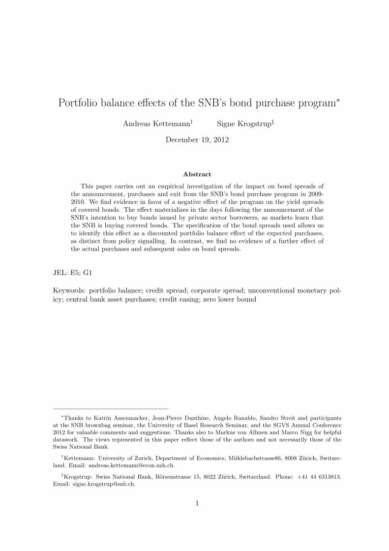
Figure 1: SNB Purchases of bonds issued by private borrowers, in million CHF. 2009

nor was any information given on which types of privately issued bonds would be purchased(covered, corporate).2 The markets thus had to learn from the subsequent actions taken bythe SNB. The SNB started to purchase bonds immediately, i.e. right after 2pm on the 12March. The vertical line in Figure 1 shows the announcement and date of first purchases on12 March 2009, and the red and black lines show purchases of covered and corporate bondsrespectively. In the first weeks after the announcement, the SNB exclusively bought coveredbonds. About three weeks later, on 6 April 2009, the SNB commenced purchases of non-bank corporate bonds in addition to continuing the purchases of covered bonds. Non-bankcorporate bond purchases remained a small part of overall purchases throughout the program.

The bond purchases took place at different times of day during the purchase period, andthe purchases continued in both bond categories until early July. No further bonds werepurchased after July. The purchases were officially discontinued in September 2009, and theprogram was announced as completed in December 2009.

The program was exited as the bonds were sold back into the market during the monthsof March to August 2010. This was a period of falling risk aversion and high demand forassets denominated in Swiss francs, notably Swiss bonds. The profile for the bond sales isdepicted in Figure 2.

The exit was not announced. The sales were carried out anonymously, and remainedlargely unnoticed. The first piece of information as to the fact that the SNB was selling offits bonds came in late August 2010 with the release of its monthly balance sheet statistics(monthly bulletin). At this time, nearly all the bond were sold off.

2A week later, on the 19th March, 2009, SNB Governing Board Member Thomas Jordan stated in a speech thatthe purpose of private bond purchases was credit easing, i.e. reduction of risk premia for private borrowersin capital markets.

4

0

50

100

150

200

250

300

M3 M4 M5 M6 M7 M8 M9

2010

SNB covered bond sales, million CHF

SNB non-bank corporate bond sales, million CHF

Figure 2: SNB sales of bonds issued by private borrowers, in million CHF. 2010

At the hight of the program, the SNB had purchased a total of about CHF 3 billion worthof assets, or about 0.5% of Swiss GDP, which is small relative to for example the FederalReserve asset purchase programs (the total assets purchased by the Federal Reserve now ex-ceed 10% of GDP). The program was not small relative to the size of the Swiss bond market,however. At the end of 2009, covered bonds on the balance sheet of the SNB amounted toabout 5% of the total market volume of covered bonds at that time, 20% of gross new issuanceand 100% of net new issuance of covered bonds in the Swiss market in 2009. The corporatebond purchases were less substantial, both in absolute and in relative terms.

How should we expect the SNB’s announcement and subsequent bond purchases to haveaffected Swiss private sector bond yields? The yield of a bond can be written as consistingof a risk neutral part as given by expected future short interest rates, and a term premium,according to:

ımt,j = RNmt + TPMm

t + TPImt,j (1)

where t is time, j is the specific issuer, and m is maturity. RNmt is the risk-neutral part

of the interest rate. The term TPMmt is a macro risk premium, capturing for example un-

certainty regarding the growth and inflation outlook, or changes in overall risk aversion. Incontrast, TPImt,j is an issuer specific risk premium, which depends on issuer specific risks suchas the risk of default of the issuer in question, risk aversion, and preferred habitat. Whereasper definition, TPImt,j differs across issuers, RNm

t and TPMmt are the same for all bonds in

the country in question.

The effect of the bond purchase program on bond yields can be divided into two broadcategories, namely the policy signaling effect and the portfolio balance effect discussed in theintroduction. First, the SNB bond purchase program could have signalled to the marketssomething about how the SNB perceived the economic situation and prospects. In turn, theprogram would have affected the market view of how the SNB intended to set short term

5

interest rates in the future. Such changes in expected future policy rates would affect RNmt .

Policy signalling effects could have occurred both at the announcement of the policy, andwhen the subsequent outright purchases took place, as both types of instances could havecontained separate new information.

Second, portfolio balance effects would arise because central bank purchases of bondsdirectly from the markets would reduce the remaining supply of such bonds in the market.Private portfolios would hence have to adjust. All else equal, a reduction in the supply ofa bond would tend to increase the price of that bond relative to the prices of other assetsaccording to theories of portfolio balance (see for example Tobin (1965), Hamilton and Wu(2010) or Vayanos and Vila (2009)). The portfolio balance effect would affect the TPImt,j partof the yield. It is possible that the TPImt,j of close substitutes to the bonds purchased by theSNB would also be affected through substitution effects.

The portfolio balance effect can occur at announcement and when the actual purchasestake place, depending on the level of information that markets have at each of these typesof events. If markets know in advance the size of the purchases, the timing and the type ofbonds to be purchased, it is reasonable to assume that some, if not all, of the portfolio balanceeffects will happen instantly, as markets discount the expected change in the price. However,in the case of the SNB bond purchase program, and as opposed to the Federal reserve andBank of England programs, this information was not revealed with the announcement on the12th March, nor at any later stage prior to the termination of the program. Markets werehence left to infer from the subsequent actions of the SNB which types of bonds would bepurchased and how much. Portfolio effects could hence have occurred both at announcementtime, and in connection with the subsequent actual purchases.

Separating the effect of the program into a policy signaling effect which affects risk-neutralrates only, and a portfolio balance effect which affects the term premium only, is of course aconvenient simplification which facilitates the empirical analysis. A few potential complica-tions should be noted, however, as they will have to be kept in mind for the specification ofthe baseline regression and controls.

First, the news that the announcement provided to the markets about the future eco-nomic outlook and the seriousness of the situation could also have affected the uncertaintyabout expected future growth and inflation outcomes, which in turn would affect TPMm

t .This could in turn have increased market risk aversion, which would have affected bondsas a function of their level of risk, and hence, TPImt,j . Moreover, if markets adjusted theirexpectations of the economic outlook when the bond purchase program was announced, thenthis could have affected the expected default risk of certain borrowers more than others, inturn affecting TPImt,j . These effects through risk aversion and expected default risk have tobe kept in mind, as we will need to control for them in our regressions.

The purchase program could also have affected the market liquidity of the purchasedbonds, which in turn could have affected their attractiveness and hence price. This marketliquidity effect (to be distinguished from the liquidity effect of higher bank reserves) wouldalso affect the issuer specific term premium of the bonds, TPImt,j . We take this possible mar-ket liquidity effect into account in the empirical specification by controlling for a measure of

6

1.2

1.6

2.0

2.4

2.8

0

500

1,000

1,500

2,000

2,500

3,000

3,500

M12 M1 M2 M3 M4 M5 M6 M7 M8 M9

2008 2009

SNB total bond purchases, cummulative, million CHF. RHS axis.

10-year yield on Confederation bonds. LHS axis.

Figure 3: The SNB bond purchases and the 10-year yield on Confederation bonds

market liquidity specific to the categories of the purchased bonds.

Finally, any unsterilized asset purchases by a central bank increases banks’ reserves andhence the money supply. In turn, more bank reserves could increase the overall demand forassets from banks, which in turn would tend to increase the price of assets, as argued inKrogstrup et al. (2012b). The effect is referred to as a liquidity effect in the traditional macroliterature (see for example Cochrane (1989)). All else equal, the liquidity effect should notdiscriminate between assets in banks’ portfolios. It could hence reduce TPMm

t , but shouldnot necessarily affect the issuer specific term premium TPImt,j . One exception is worth men-tioning. Empirically, liquidity effects have mainly been found in the yields of highly liquidand safe bonds such as government bonds. It could hence be that the liquidity created by thebond purchases would have had the effect of reducing Confederation bond yields more thanthe yields of other bonds. If so, this would not be a problem for our identification strategyhere, as explained in Section 5.2. Note that there is no reason to expect liquidity effects ofthe bond purchase program itself to have been important in Switzerland, given the relativelysmall size of the program, as well as the high level of bank reserves already in the system atthis time due to other unconventional policy measures. Just as is the case for the portfoliobalance effect, liquidity effects could occur at announcement as well as at the actual bondpurchase times, depending on the market’s level of information at these events. Except for afall at the announcement of the policy package on the 12th March 2009, Confederation bondyields did not in fact fall during the period in which the SNB was buying bonds, see Figure3.

The discussion of the different effects of the bond purchase program implies that if weisolate TPImt,j in the data, and associate it with the announcement time of the SNB bondpurchase program as well as the dates of the subsequent actual bond purchases, and correctlycontrol for changes in risk aversion, market liquidity and expected default risk, then any re-maining significantly negative correlation with the bond purchases or with the announcementof the bond purchase program should indicate portfolio balance effects.

7

3 A measure of the issuer specific term premium: The creditspread

Based on Equation (1), we compute the issuer specific term premium as the spread of theyield on any individual bond over the yield on the corresponding maturity Confederationbond.

CSmt,j = imt,j − imt,conf

= TPImt,j − TPImt,conf (2)

We then assume that TPImt,Conf is orthogonal to the SNB’s bond purchases. As discussedabove, liquidity effects of the bond purchases could affect the Confederation bond specificterm premium, but such an effect would only bias our results downward. Apart from liq-uidity effects, the assumption of an orthogonal TPImt,Conf is reasonable in light of the liquidmarket for Confederation bonds and the very low default risk of these bonds. In order to geta smooth series for the credit spread over time, we take a weighted average of these bondspecific term premia across categories of bonds traded in the Swiss bond market, to get creditindices for covered bonds, domestic non-bank corporates, cantonal bonds and bank bonds.The first two are the focus of this analysis. The latter two indices are used for comparisonbelow.

The credit indices are derived from individual bond yield-to-maturity spreads over SwissConfederation bonds of the same maturity (the latter interpolated using a spline), aggregatedaccording to the emission volume of the bond in question, and across all maturities.3 Bothindices are based on a sufficiently large set of observations for every point in time to be repre-sentative of overall market conditions. The resulting series for covered and corporate bonds,as well as an index comprising all bonds in the Swiss bond market, are depicted in Figure 4.

4 Event study approach

The daily credit indices offer interesting insights into how spreads evolved during the periodwhen the SNB bond purchase program was active. We start with an investigation of the onsetand purchase period in the spring and summer of 2009.

4.1 The announcement and the bond purchases in 2009

Figures 5 to 9 depict the credit indices of four bond categories together with the SNB bondpurchases. The two vertical lines in the Figures denote, first, the announcement of the pro-gram and beginning of the covered bond purchases on the 12th March, and second, the onsetof the more moderate industrial bond purchases on the 6th April 2009, respectively.

3The averaging over different maturities could cause the credit index to be correlated with the average time-to-maturity in the market. However, the mean time-to-maturity shows little variation over time and is neversignificant in the various regressions we conduct.

8

0.0

0.5

1.0

1.5

2.0

2.5

3.0

0.0

0.5

1.0

1.5

2.0

2.5

3.0

00 01 02 03 04 05 06 07 08 09 10 11

The Credit Index for Swiss Bonds

The Credit Index for non-bank corporate issuers

The Credit Index for Covered Bonds (pfandbriefe)

Figure 4: The credit index for total, covered and corporate bonds

Figure 5 shows that there was no visible effect of the SNB announcement on 12th March2009 on corporate bond spreads. One possible reason could be that market participants didnot know what the SNB meant by ”bonds of private borrowers” and hence did not react bychanging their demand for corporate bonds at announcement. Instead, the corporate creditindex started declining on the 2nd April 2009, a few days before the SNB started outrightpurchases of non-bank corporate bonds on the 6th April. From pure visual inspection, how-ever, it is not clear that this decline was related to the bond purchase program.4

Figure 6 shows that the spread on covered bonds at first did not react to the announce-ment. Zooming in on the weeks surrounding the announcement of the program, Figure 7shows that the spread remained steady in the days following announcement, i.e. on the 13thand 14th of March. The spread then dropped by about 10bp on the third day, and a fewmore basis points in the following days, i.e. between the 16th and 19th March 2009.

Neither corporate bond spreads, nor the spreads for cantonal bonds and bank bonds de-picted in Figures 8 and 9 saw falling spreads in the days following the SNB announcement.On the contrary, spreads for other bond categories increased. The strong fall in covered bondspreads is hence particular to covered bonds rather than a change in overall market conditionsor sentiment.

Rather than a portfolio balance effect, could the drop in the covered credit spread reflecta lower liquidity risk premium due to an increase in market liquidity triggered by the factthat the SNB entered this particular market? This is not likely according to Figure 10. Asa proxy for the the daily liquidity of the covered bond market, Figure 10 plots a weightedaverage of daily bid-ask spreads of the bonds that enter the credit index, together with thecovered credit spread and the date for the announcement of the program. A narrower bid-ask

4A speech was given by the president of the SNB governing board, Philipp Hildebrand, on the 2nd April 2009,in which he stressed the bond purchase program and what the SNB intended with this program. Whether ornot this information was important for the spread is difficult to assess.

9

0.9

1.0

1.1

1.2

1.3

1.4

1.5

1.6

1.7

0

50

100

150

200

250

300

350

400

M12 M1 M2 M3 M4 M5 M6 M7 M8 M9

2008 2009

SNB non-bank corporate bond purchases, cummulative, million CHF. RHS axis.

Credit spread on non-bank corporate bonds. LHS axis.

Figure 5: Daily non-bank corporate credit index and cumulated SNB non-bank corporate bondpurchases, levels

.0

.1

.2

.3

.4

.5

0

400

800

1,200

1,600

2,000

2,400

2,800

3,200

M12 M1 M2 M3 M4 M5 M6 M7 M8 M9

2008 2009

SNB covered bond purchases, cummulative, million CHF. RHS axis.

Credit spread on covered bonds. LHS axis.

Figure 6: Daily covered bond credit index and the SNB covered bond purchases, levels

10

.16

.20

.24

.28

.32

.36

.40

0

400

800

1,200

1,600

2,000

2 4 6 10 12 16 18 20 24 26 30 1 3 7 9 13 15 17 21 23 27 29

M3 M4



Figure 7: Daily covered bond credit index and the SNB covered bond purchases, levels

.0

.1

.2

.3

.4

.5

0

500

1,000

1,500

2,000

2,500

3,000

3,500

M12 M1 M2 M3 M4 M5 M6 M7 M8 M9

2008 2009


Credit spread on cantonal bonds. LHS axis.

Figure 8: Daily cantonal bond credit index and the SNB total bond purchases, levels

11

.0

.1

.2

.3

.4

.5

.6

.7

0

500

1,000

1,500

2,000

2,500

3,000

3,500

M12 M1 M2 M3 M4 M5 M6 M7 M8 M9

2008 2009


Credit spread on bank bonds. LHS axis.

Figure 9: Daily bank bond credit index and the SNB total bond purchases, levels

spread should reflect higher liquidity. If anything, however, market liquidity in the coveredbond market seems to have decreased in the days following the announcement of the bondpurchase program.

Finally, Figure 11 shows the movement of 10-year Confederation bond yields around thetime of the announcement of the SNB bond purchase program. Yields dropped in the daysafter the announcement, which could reflect changes in all three components of the yield.The drop suggests that the fall in the credit spread on covered bonds in the days after theannouncement came in spite of a drop in risk free rates, i.e. covered bond yields fell evenmore than risk free yields.

4.2 The unannounced bond sales in 2010

Just as for purchases, we would expect the bond sales in 2010 to have had an effect on creditspreads if central bank open market operations have portfolio balance effects. Contrary to theannounced purchases, however, we would expect the effects of the unannounced sales to occuras a consequence of the actual sales, rather than being discounted by market participants in anannouncement effect. Figures 12 to 13 show the covered and corporate bond credit spreadsand the SNB holdings of the corresponding bonds during the period of the sales in 2010respectively. The Figures show very little sign of an increase in bond spreads as a result ofthe sales. There is no clear direct reaction of the spread to the sales, and spreads tend todecline rather than increase over the time period.

4.3 Conclusions from the event analysis

The event analysis suggests that when the markets had observed the SNB’s purchases of cov-ered bonds in the days following the announcement of the program, the plausible portfoliobalance effect of the SNB’s total expected purchases was discounted in a decline in the coveredbond spread of between 10 and 12 basis points. No such effect was observed in the spread forcorporate bonds or any other bond category for that matter. Spreads generally declined in

12

0.4

0.8

1.2

1.6

2.0

0

400

800

1,200

1,600

2,000

2 9 16 23 2 9 16 23 30 6 13 20 27

M2 M3 M4


Liquidity in the covered bond market (average bid-ask spread). LHS axis.

Liquidity in the confederation bond market (average bid-ask spread). LHS axis.

Credit spread for covered bonds. LHS axis.

Figure 10: Covered credit spread, market liquidity and SNB bond purchases

.15

.20

.25

.30

.35

.40

.45

.50

2.00

2.05

2.10

2.15

2.20

2.25

2.30

2.35

2 4 6 10 12 16 18 20 24 26 30 1 3 7 9 13 15 17 21 23 27 29

M3 M4

10-year Confederation bond yields. RHS axis.


Figure 11: Covered credit spread and Confederation bond yields around the SNB announcement

13

.00

.05

.10

.15

.20

.25

.30

.35

.40

0

500

1,000

1,500

2,000

2,500

3,000

3,500

M1 M2 M3 M4 M5 M6 M7 M8 M9 M10 M11

2010

SNB covered bond sales, cummulative, million CHF. RHS axis.


Figure 12: Daily covered credit index and the SNB covered bond sales, levels (holdings)

0.7

0.8

0.9

1.0

1.1

1.2

1.3

0

100

200

300

400

M1 M2 M3 M4 M5 M6 M7 M8 M9 M10 M11

2010

SNB corporate bond sales, cummulative, million CHF. RHS axis.

Credit spread on corporate bonds. LHS axis.

Figure 13: Daily corporate credit index and the SNB corporate bond sales, levels (holdings)

14

the months following the first purchases, as we would expect from a further portfolio balanceeffect on spreads. In contrast, spreads also slightly declined during the period of the bondsales, whereas a portfolio balance effect of the sales should generate an increase in spreads. Itis hence not clear from the data that portfolio balance effects were present beyond the initialdiscounted effect in the days following the announcement.

While these visual impressions are suggestive, no firm conclusions can be drawn on causal-ity between the SNB bond purchase program and credit spread from the figures alone.5 First,we need to investigate whether the decline in the covered spread in the days after the an-nouncement of the program was statistically significant. Moreover, we also need to controlfor movements in other factors during the period in question. In particular, we need to as-sess whether the subsequent bond purchases and sales might have had independent effects oncredit spreads aside from the announcement, when controlling for the main determinants ofSwiss credit spreads. We hence turn to econometric analysis of the bond purchase program.

5 Econometric investigation

We carry out regressions for the credit index for covered and non-bank corporate bondsrespectively, on determinants of credit spreads as well as on the SNB bond purchases and sales.The sample period is September 2000 to December 2010. We use daily data, which allowsus to carefully assess the effect of the announcement of the program and possible immediateeffects of purchases on bond markets. The regressions are estimated in first differences so asto circumvent non-stationarity problems (the credit spread has a unit root, whereas the firstdifference is stationary). The baseline regression specification is in line with the literature,e.g. Collin-Dufresne et al. (2001) and Avramov et al. (2007). It should be noted that portfoliobalance effects of the actual purchases could materialize with a longer delay that what wecan allow for in a daily first differences specification. However, it is more difficult to establishcausality in levels regressions and regressions using weekly or monthly frequency. We henceonly do so as a robustness check. The baseline specification becomes:

∆cit =α+ βvolvolt + βSPI∆SPIt−1 + βsnb∆SNBbt + βdcov∆Dsnbcovt−1

+ βdcorp∆Dsnbcorpt−1 + βTS∆TSt + βR∆R10y

t + βBA∆BidAskt + ut, (3)

cit is the relevant credit index, and ∆SNBbt captures the actual monthly purchases (+)and sales (-) of corporate and covered bonds effected by the SNB in the period between Marchand December 2010. We include the contemporaneous purchases and sales as well as a lag.The lag is included in order to allow for all purchases or sales that have taken place after thetime of the recording of the credit spread (morning) to have an effect on the credit spread theday after. The purchases and sales are measured in percent of the corresponding bond cate-gory’s emission volumes. Dsnbcov

t is a dummy for the date of the announcement of the SNBpurchase program and the date of the first covered bond purchases. It is included to captureboth the effects of the announcement on spreads, and the effects of the markets’ learning that

5This point is made by Stroebel and Taylor (2009) in a general critique of the event analysis approach toassessing the effects of the various asset purchase programs conducted by the Federal Reserve since the onsetof the financial crisis.

15

the SNB is buying covered bonds. We include three lags of this dummy in the regressionusing daily data, in order to capture residual movements in covered bond spreads during thedays following the announcement. The choice of three daily lags of the announcement dummyallows us to test whether the strong fall in the covered bond spread after three days of theannouncement is significant when controlling for other determinants of the spread. We donot include the contemporaneous announcement dummy, because the press release and firstpurchases were made in the afternoon of the 12th of March, whereas the data used for thecalculation of the credit spread is collected in the morning. For consistency, we also includethree lags of a second dummy, Dsnbcorp

t , which captures the date of the first corporate bondpurchases on the 6th of April 2009. This dummy captures effects on spreads of the marketslearning that the SNB has entered the non-bank corporate market.

The control variables are the following. volt is the conditional stock price volatility esti-mated during the sample period, included to control for a link between credit spreads andhigh volatility periods (risk aversion). SPIt is a measure of expected loss due to default,which we - following the previous literature - proxy by the log of the level of the main Swissstock price index, the SPI. Note that the SPI also captures the overall performance of theeconomy. Volatility and the SPI are lagged one day to account for the fact that the data forthese variables are collected at market close while the data on credit spreads are collectedduring the morning. All other daily variables are collected during the morning, and henceincluded as contemporary variables only.

In order to control for changes in market liquidity around the announcement and purchasetimes, we include the average emission-volume-weighted bid-ask spread of the bond categoryin question less the average emission-volume-weighted bid-ask spread for confederation bonds.The bid-ask spread is based on data on bid and ask prices from the same daily dataset onthe Swiss bond market used to compute the credit index. The average bid-ask spreads arehence consistent with the credit index in terms of types of bonds included in the differentcategories, the time of day at which the data are collected in the market, and how it relates tothe confederation bond market. The liquidity measure is described in Krogstrup et al. (2012a).

Macroeconomic developments are further controlled for by including the long term interestrate level, i.e. the 10-year Confederation bond yield R10y

t . Its empirical prior is negative (seeCollin-Dufresne et al. (2001)). A higher level of interest rates reflects a strong business cycledevelopments, which is good for firm profitability. Finally, we follow Fama and French (1989)and include the term spread, TSt, defined as the difference between the 10-year Confederationbond yield and the three-month CHF libor. A higher term spread could be taken to signalhigher uncertainty about future economic outcomes, suggesting a positive relation with creditspreads.

5.1 Regression results

Table 1 presents the results for the baseline regression using daily data for covered and non-bank corporate spreads in column one and two. Most control variables have the correct signs,and the term spread and the long-term bond yield are significant.

16

Confirming the visual impressions of Section 4, the third lag of the announcement andpurchases dummy for covered bonds is significantly negative in the covered bond spread re-gression, suggesting that the spread declined by about 10-12 basis points on that day withoutany of the control variables included in the regression being able to account for that. Thedecline is significantly different from zero at the 1% level. It is hence plausible that it is theresult of the markets’ evolving perception regarding the SNB intentions of purchasing coveredbonds.

The results also confirm that the announcement did not affect corporate bonds to thesame degree. The second lag after announcement is significantly negative, while the third lagis positive. None of the estimated parameters for the lags are of an economically relevantsize. The same lack of economic relevance holds true for the dummy for the beginning of thecorporate bond purchases on the 6th April 2009.

Turning to the parameter estimates for the outright bond purchases and sales of the SNB,these come with the expected negative sign, but they are insignificant in both regressions.The data thus does not support the hypothesis that there were additional immediate portfoliobalance effects associated with the outright purchases and sales. Using a dummy taking thevalue one from January 2010 onwards, the specification in Table 2 allows the effects of thepurchases and the effects of the sales in 2010 to differ. Again, neither the purchases nor thesales have significant effects on credit spreads.

The lack of an effect of the outright bond market interventions could reflect the efficientmarkets hypothesis that the effect of the purchases was discounted in the price of coveredbonds as soon as the markets has realized that the SNB would be buying covered bonds.This interpretation implies that markets know what the aggregate portfolio balance effect ofthe purchases would be, without knowing how much and for how long the SNB intended tobuy, which seems unlikely. Alternatively, the lack of an effect of the interventions would alsobe consistent with the view that markets discounted an expected effect of the interventions,which didn’t actually materialize.

In conclusion, the data supports the hypothesis that there was an announcement effectof the first covered bond purchases on the spreads of covered bonds. However, there is noevidence in the data of an economically relevant effect of the bond purchase program on cor-porate bonds.

5.2 Robustness

Tables 4 to 8 display the results of a series of robustness tests. First, the bond traders at theSNB are likely to have adjusted their purchases according to the market conditions of thepurchased bonds. For example, it is possible that covered bonds were purchased at a largerquantity on days where prices of these were going down and yields up, as it was the intentionof the SNB to reduce the yield spreads. Similarly, it is likely that more bonds were sold ondays when the prices of the bonds were increasing and yields falling, during the sales periodin 2010. This suggests a source of endogneity of the SNB’s bond market interventions whichwould tend to bias the parameter estimates of the regressions downward. There are two ways

17

of addressing this type of endogeneity in the literature (see references to investigations of theECB’s SMP, non-published papers). One way is to investigate intra-day high-frequency data.We do not have intra-day data on credit spreads. The second option is to use instruments.We are not aware of any good instrumental variable for SNB bond market interventions. Asa second-best option, we carry out a TSLS regression using lags of the explanatory variablesas instruments. We instrument bond purchases and sales and their first lag with their 2ndand 3rd lags. The results are given in Table 3. As could be expected, standard errorsincrease strongly, but all coefficients that stay significant keep the right sign. The conclusionsfrom using instruments are largely the same as those from standard regressions. The actualbond purchases and sales did not systematically affect credit spreads. In lack of appropriateinstruments, however, it is not possible to make any firm conclusions on the lack of an effect.

Second, Table 4 shows that a longer average maturity of outstanding total bonds is foundto significantly reduce the covered credit spread. However, the inclusion of average maturitydoes not affect the conclusions from the baseline regressions. It should be added that noredemptions or new issues of covered bonds took place during the week after the announce-ments of the bond purchase program, and hence, that there was no exceptional variation inthe average maturity in those days.

Third, in the months and year after the announcement of the SNB bond purchase program,corporate spreads generally declined in western countries. This was a period of increasing calmin global financial markets. Could the decline in the covered spread following the announce-ment of the bond purchase program have reflected a more general decline in internationalcorporate spreads? Table 5 shows that controlling for movements in different types of US andEuropean corporate spreads do not change the findings. The foreign spreads used here arenot even significant in explaining daily changes in Swiss covered and corporate spreads.

Fourth, Table 6 shows the regression results when controlling for the market liquidityof the purchased bonds. The results confirm the conclusions derived from Figure 10. Theaverage bid-ask spread as a proxy for market liquidity is not significant and its inclusion doesnot change the finding that the covered credit spread fell significantly in the days followingthe announcement.

Fifth, Table 7 uses a different proxy for risk aversion, namely the spread between the3-month Libor and the 3-month term overnight interest swap rate. The change of controlvariable is inconsequential for the significance of the relevant parameter estimates.

Further, the distribution of credit spreads tend to have fat tails. We hence allow fortime varying variation by estimating a Garch(1,1) specification using maximum likelihoodtechniques. The GARCH specification becomes:

∆cit =α+ βσσ2t + βSPI∆SPIt−1 + βsnb∆SNBbt + βdcov∆Dsnbcov

t−1

+ βdcorp∆Dsnbcorpt−1 + βTS∆TSt + βR∆R10y

t + βBA∆BidAskt + ut, (4)

σ2t =ω + αu2t−1 + βσ2

t−1, (5)

18

ut|Ft−1 ∼ N (0, σ2t ), (6)

where Ft−1 is the information set in period t-1. Results for the estimation of this specifi-cation, given in Table 8, confirm the results from the baseline specification.

Finally, the lack of significance of the actual bond purchases and sales in the credit spreadregressions could be taken to reflect the daily frequency of the data used and/or the use offirst differences. We find that this is not the case. In regressions in levels, with and withouta lagged dependent, the outright purchases and sales remain largely insignificant (not shown).6

6 Conclusions

This paper has investigated the impact of the SNB bond purchase program of 2009-2010 onSwiss corporate spreads, and found evidence suggesting a moderate effect of the announce-ment of the bond purchases on the credit spreads of covered bonds in the order of about 10-12basis points. The effect materialized in the days following the announcement of the programand first bond purchases. Subsequent actual bond purchases had no further effect on spreads.Moreover, there was no evidence in the data of an effect of the program on corporate bondspreads. Finally, the unannounced bond sales in 2010 did not affect the spreads of the soldbond categories. Markets were not aware of the sales until they were largely over, and thebonds were sold off during a period of low risk aversion and high demand for bonds.

The design of the empirical investigation allows us to plausibly identify the announcementeffect on covered spreads as the market discounting an expected portfolio balance effect ofthe SNB bond purchases. It also allows us to characterize the effect as a lower bound for thetotal effect of the bond purchase program on bond yields. Thus, the actual bond purchasescould have had portfolio balance effects on spreads beyond those we identify, if, for example,such effects materialized with a delay of more than a few days, of if the effects on spreadswere irregular, for example due to variable lags. The data and our empirical strategy doesnot allow us to pick up such delayed or irregular effects. In addition, the bond purchaseprogram could have had signaling effects on expected future policy and short term interestrates. Signalling effects would not appear in the spreads we investigate, but rather in yieldsdirectly. The data we use does not allow us to identify such effects.

The findings suggest more generally that central bank asset purchases programs are proba-bly perceived by the market as having portfolio balance effects, whether or not such portfoliobalance mechanisms are really active. These expected effects are then discounted in theprices of the purchased assets at announcement and/or at the onset of the purchase program,depending on the level of information offered at the announcement of the program. One

6There is an exception, in that the outright corporate bond purchases turn significant in some specifications.But when this is the case, the contemporaneous and lagged effects cancel out. Moreover, the finding is notrobust. The results from the levels regressions show clear signs of misspecification, with high autocorrelationand very instable parameter estimates. Results from the levels regressions are available from the authors.

19

implication is that the way in which bond purchase programs and their exit are announcedand communicated is central to the effect the central bank achieves.

20

References

Avramov, D., G. Jostova, and A. Philipov, “Understanding changes in corporate creditspreads,” Financial Analysts Journal, 2007, 63 (2), 90–105.

Bauer, Michael D. and Glenn D. Rudebusch, “The Signaling Channel for FederalReserve Bond Purchases,” Federal Reserve Bank of San Francisco Working Paper Series,No. 21, 2011.

Cochrane, John H, “The Return of the Liquidity Effect: A Study of the Short-run Relationbetween Money Growth and Interest Rates,” Journal of Business & Economic Statistics,1989, 7 (1), 75–83.

Collin-Dufresne, P., R.S. Goldstein, and J.S. Martin, “The determinants of creditspread changes,” The Journal of Finance, 2001, 56 (6), 2177–2207.

Fama, E.F. and K.R. French, “Business Conditions and Expected Returns on Stocks andBonds,” Journal of Financial Economics, 1989, 25 (1), 23–49.

Gagnon, Joseph, Matthew Raskin, Julie Remache, and Brian Sack, “Large-scaleasset purchases by the Federal Reserve: did they work?,” Staff Reports 441, Federal ReserveBank of New York 2010.

Hamilton, James D. and Jing (Cynthia) Wu, “The Effectiveness of Alternative Mon-etary Policy Tools in a Zero Lower Bound Environment,” Working Paper, University ofCalifornia, San Diego 2010.

Joyce, Michael, Matthew Tong, and Robert Woods, “The United Kingdom’s quanti-tative easing policy: design, operation and impact,” Bank of England Quarterly Bulletin,2011, 3.

Krogstrup, Signe, Marco Nigg, and Markus von Allmen, “A new measure of liquidityin the Swiss bond market,” Memo, Swiss National Bank 2012.

, Samuel Reynard, and Barbara Sutter, “Liquidity effects at the Zero Lower Bound,”SNB Working Paper, 2012, (2).

Neely, Christopher J., “The large scale asset purchases had large international effects,”Working Papers 2010-018, Federal Reserve Bank of St. Louis 2010.

Stroebel, Johannes C. and John B. Taylor, “Estimated Impact of the Feds Mortgage-Backed Securities Purchase Program,” NBER Working Paper, 2009, (15626).

Tobin, James, “The theory of portfolio selection,” in Hahn and Brechling (eds.): The theoryof interest rates, 1965, pp. 3–52.

Vayanos, Dimitri and Jean-Luc Vila, “A Preferred-Habitat Model of the Term Structureof Interest Rates,” NBER Working Papers 15487, National Bureau of Economic Research,Inc 2009.

21

7 Appendix: The data

7.1 Source and description of the data

The data source for all data used in this analysis is the SNB.

7.2 Volatility data

The conditional volatility used in the analysis is obtained by estimating a standardGARCH(1, 1)model on the daily log-returns of the SPI.

7.3 Average rating index

We combine rating classes from different sources. The following order is used, where latersources act as substitutes if the previous ones are unavailable:

1. Standard & Poor’s

2. Moody’s

3. Fitch

4. Zuercher Kantonalbank

For the average rating index, we had to translate qualitative rating criteria into quan-titative information. This is accomplished by numbering consecutively through all ratingcategories as shown in Table 10 and taking an emission volume weighted average of the re-sulting values. This conversion is valid given the assumption that differences in credibilitybetween adjacent rating categories are approximately constant.

22

Table 1: Baseline regression results

Covered Bonds Corporate Bonds(1) (2)

∆SNBbcovt 1.032(.695)

∆SNBbcovt−1 -.652(.782)

∆SNBbcorpt -1.442(4.849)

∆SNBbcorpt−1 1.449(4.628)

∆volt−1 · 100 -.149 -.105(.171) (.261)

∆logSPIt−1 -.053 -.032(.040) (.069)

∆TSt .094 .146(.032)∗∗∗ (.054)∗∗∗

∆R10yt -.195 -.381

(.033)∗∗∗ (.058)∗∗∗

∆BidAskt .002 .004(.003) (.005)

Dsnbcovt−1 .002 .002

(.002) (.004)

Dsnbcovt−2 .001 -.006

(.002) (.002)∗∗∗

Dsnbcovt−3 -.098 .017

(.002)∗∗∗ (.002)∗∗∗

Dsnbcorpt−1 -.027 -.030

(.001)∗∗∗ (.009)∗∗∗

Dsnbcorpt−2 .012 .010

(.001)∗∗∗ (.011)

Dsnbcorpt−3 -.011 .019

(.001)∗∗∗ (.002)∗∗∗

Const. .000 .000(.000) (.001)

Obs. 2307 2302R2 .058 .079

Notes: The sample period is September 1st, 2000, until December 31th, 2010. The numbers in parentheses areheteroskedasticity- and autocorrelation-consistent (Newey-West) standard errors.∗ p < 0.10, ∗∗ p < 0.05, ∗∗∗ p < 0.01.

23

Table 2: Baseline with an interaction dummy for bond sales


∆SNBbcovt .902(1.121)

∆SNBbcovt−1 -.487(1.104)

∆SNBbcovt × Salet .223(1.424)

∆SNBbcovt−1 × Salet−1 -.308(1.578)

∆SNBbcorpt -4.782(7.358)

∆SNBbcorpt−1 -1.966(10.305)

∆SNBbcorpt × Salet 6.841(7.483)

∆SNBbcorpt−1 × Salet−1 4.013(10.546)


(.003) (.004)

Dsnbcovt−2 .000 -.006

(.003) (.002)∗∗∗

Dsnbcovt−3 -.098 .017

(.003)∗∗∗ (.002)∗∗∗

Dsnbcorpt−1 -.027 -.011

(.001)∗∗∗ (.019)


(.001)∗∗∗ (.026)


(.002)∗∗∗ (.004)∗∗∗

Obs. 2307 2302R2 .058 .079

Notes: The sample period is September 1st, 2000, until December 31th, 2010. The numbers in parentheses areheteroskedasticity- and autocorrelation-consistent (Newey-West) standard errors.∗ p < 0.10, ∗∗ p < 0.05, ∗∗∗ p < 0.01.

24

Table 3: TSLS regression


∆SNBbcovt -44.896(112.803)

∆SNBbcovt−1 39.911(102.295)

∆SNBbcorpt 30.824(42.181)

∆SNBbcorpt−1 -27.126(40.102)


(.026) (.004)

Dsnbcovt−2 -.056 -.006

(.149) (.002)∗∗∗

Dsnbcovt−3 -.001 .017

(.233) (.002)∗∗∗

Dsnbcorpt−1 .017 -.047

(.107) (.022)∗∗


(.049) (.091)


(.109) (.011)∗∗

Obs. 2129 2124R2 .055 .075

Notes: The sample period is September 1st, 2000, until December 31th, 2010. The numbers in parentheses areheteroskedasticity and autocorrelation consistent (Newey-West) standard errors.∗ p < 0.10, ∗∗ p < 0.05, ∗∗∗ p < 0.01.

25

Table 4: Controlling for the average maturity of the bonds within the given category


∆SNBbcovt 1.006(.695)

∆SNBbcovt−1 -.654(.777)

∆SNBbcorpt -1.442(4.845)

∆SNBbcorpt−1 1.433(4.635)

∆volt−1 · 100 -.148 -.105(.170) (.261)

∆logSPIt−1 -.052 -.032(.040) (.069)

∆TSt .092 .147(.033)∗∗∗ (.054)∗∗∗

∆R10yt -.193 -.381

(.033)∗∗∗ (.058)∗∗∗

∆BidAskt .002 .004(.003) (.005)

∆logMatpft -.771 .088(.289)∗∗∗ (.415)


(.002) (.004)

Dsnbcovt−2 .001 -.006

(.002) (.002)∗∗∗

Dsnbcovt−3 -.098 .017

(.002)∗∗∗ (.002)∗∗∗

Dsnbcorpt−1 -.027 -.029

(.001)∗∗∗ (.009)∗∗∗


(.001)∗∗∗ (.011)


(.001)∗∗∗ (.002)∗∗∗

Const. .000 .000(.000) (.001)

Obs. 2307 2302R2 .059 .079


26

Table 5: Controlling for foreign spreads


∆SNBbcovt 1.281(.746)∗

∆SNBbcovt−1 -.707(.799)

∆SNBbcorpt -1.054(4.705)

∆SNBbcorpt−1 1.092(4.729)

∆volt−1 · 100 -.155 -.114(.182) (.257)

∆logSPIt−1 -.044 -.009(.040) (.075)

∆TSt .093 .144(.032)∗∗∗ (.055)∗∗∗

∆R10yt -.194 -.376

(.033)∗∗∗ (.058)∗∗∗

∆BidAskt .003 .004(.003) (.005)

∆CorpHLust -.022 -.012

(.018) (.017)

∆CorpHLeut .022 .043

(.015) (.030)


(.003) (.004)


(.009) (.008)

Dsnbcovt−3 -.095 .019

(.004)∗∗∗ (.004)∗∗∗

Dsnbcorpt−1 -.028 -.029

(.001)∗∗∗ (.008)∗∗∗


(.001)∗∗∗ (.012)


(.002)∗∗∗ (.002)∗∗∗

Const. .000 .000(.000) (.001)

Obs. 2307 2302R2 .061 .082

Notes: The sample period is September 1st, 2000, until December 318th, 2010. The numbers in parenthesesare heteroskedasticity and autocorrelation consistent (Newey-West) standard errors.∗ p < 0.10, ∗∗ p < 0.05, ∗∗∗ p < 0.01.

27

Table 6: Including liquidity measures for Confederation, Covered and Corporate bonds separately


∆SNBbcovt .992(.699)

∆SNBbcovt−1 -.708(.783)

∆SNBbcorpt -1.482(4.880)

∆SNBbcorpt−1 1.509(4.630)

∆volt−1 · 100 -.153 -.120(.172) (.264)

∆logSPIt−1 -.055 -.039(.040) (.070)

∆TSt .088 .157(.037)∗∗ (.056)∗∗∗

∆R10yt -.176 -.383

(.037)∗∗∗ (.060)∗∗∗

∆BidAskcovt -.007 .000(.006) (.004)

∆BidAskconft .000 -.002(.005) (.008)


(.003)∗ (.004)

Dsnbcovt−2 .002 -.006

(.002) (.002)∗∗

Dsnbcovt−3 -.096 .017

(.002)∗∗∗ (.002)∗∗∗

Dsnbcorpt−1 -.028 -.030

(.002)∗∗∗ (.009)∗∗∗


(.001)∗∗∗ (.011)


(.002)∗∗∗ (.002)∗∗∗

Const. .000 .000(.000) (.001)

Obs. 2179 2179R2 .051 .077


28

Table 7: Controlling for LibTois


∆SNBbcovt .846(.725)

∆SNBbcovt−1 -.622(.784)

∆SNBbcorpt -.707(4.910)

∆SNBbcorpt−1 -.249(4.794)

∆LibToist−1 · 100 .039 .033(.027) (.037)

∆logSPIt−1 -.053 -.015(.041) (.071)

∆TSt .079 .134(.031)∗∗ (.052)∗∗

∆R10yt -.177 -.371

(.031)∗∗∗ (.056)∗∗∗

∆BidAskt .003 .004(.003) (.006)


(.002)∗ (.003)

Dsnbcovt−2 .003 -.004

(.002) (.002)∗∗

Dsnbcovt−3 -.096 .017

(.002)∗∗∗ (.002)∗∗∗

Dsnbcorpt−1 -.027 -.027

(.001)∗∗∗ (.010)∗∗∗


(.001)∗∗∗ (.012)


(.001)∗∗∗ (.002)∗∗∗

Const. .000 .000(.000) (.001)

Obs. 2167 2162R2 .06 .082


29

Table 8: GARCH estimates: conditional volatility (OIM)


∆SNBbcovt 1.201(.823)

∆SNBbcovt−1 -1.257(.841)

∆SNBbcorpt -1.226(3.759)

∆SNBbcorpt−1 3.599(3.473)

σ2 -.030 -.041(.050) (.037)

∆logSPIt−1 -.022 -.064(.033) (.045)

∆TSt .045 .102(.023)∗ (.036)∗∗∗

∆R10yt -.126 -.308

(.024)∗∗∗ (.037)∗∗∗

∆BidAskt .001 .002(.002) (.003)


(.014) (.031)

Dsnbcovt−2 .002 -.003

(.014) (.015)

Dsnbcovt−3 -.098 .019

(.013)∗∗∗ (.014)

Dsnbcorpt−1 -.027 -.035

(.011)∗∗ (.017)∗∗


(.010) (.015)


(.009) (.011)

Const. .001 .001(.001) (.001)

α .349 .468(.057)∗∗∗ (.103)∗∗∗

β .541 .621(.095)∗∗∗ (.135)∗∗∗

ω .000 .000(.000)∗ (.000)

df 4.416 2.781(.398)∗∗∗ (.165)∗∗∗

Obs. 2307 2302

Notes: The sample period is September 1st, 2000, until December 31th, 2010. The numbers in parentheses areobserved information matrix standard errors.∗ p < 0.10, ∗∗ p < 0.05, ∗∗∗ p < 0.01.

30

Table 9: Data

Acronym Explanation

cit Credit index total. Based on bond data collected dailybetween 9 and 11am.

ciindt Credit index non-bank corporate issuers.

cipft Credit index covered bonds.

BidAskpft Average emissions-weighted bid-ask spread in the mar-ket for covered bonds less that for confederationbonds. SNB-internal computations.

BidAskindt Average emissions-weighted bid-ask spread in the mar-ket for non-bank corporate bonds less that for confed-eration bonds. SNB-internal computations.

CorpHLjt Spread between BBB and AAA rated corporate debt,

j = EU,US.(add source)Dsnb

t Dummy for the zero lower bound period (zero before17 March 2009, 1 afterwards).

LibToist Spread between Swiss 3M Libor and TOIS. 3M Li-bor is collected daily at 11am in London (12am inZurich).TOIS is collected at 11am in Zurich.

Matt Mean time-to-maturity of outstanding bonds. Basedon bond data collected daily between 9 and 11am.

R10yt Zero coupon yield on 10 year government bond. Based

on bond data collected daily between 9 and 11am.Ratt Mean rating of outstanding bonds. Based on bond

data collected daily between 9 and 11am.SNBbt Cumulated purchases of bonds by the SNB, market

value, in percent of emissions volume.SNBbindt Cumulated purchases of non-bank corporate bonds by

the SNB, market value, in percent of emissions vol-ume.

SNBbpft Cumulated purchases of covered bonds by the SNB,market value, in percent of emissions volume.

SPIt Total returns on the Swiss Performance Index. Col-lected daily at market close.

TSt Term spread between 10 year and 2 year zero couponyields on government bonds. Based on data collectedbetween 9am and 11am daily.

V IXCHt VIX, implicit 30 days ahead option based volatility of

SPI. Collected daily at market close.V IXUS

t VIX for the US, Chicago board of exchange.volt Conditional volatility of the SPI, GARCH(1, 1).

Based on data collected daily at market close.

31

Table 10: Conversion of rating categories

Rating categories Number

AAA Aaa 1AA+ Aa1 2AA Aa2 3AA− Aa3 4A+ A1 5A A2 6A− A3 7BBB+ Baa1 8BBB Baa2 9BBB− Baa3 10BB+ Ba1 11BB Ba2 12BB− Ba3 13B+ B1 14B B2 15B− B3 16CCC+ Caa1 17CCC Caa2 18CCC− Caa3 19CC Ca 20C 21D 22

32

Documents

Portfolio balance effects of the SNB's bond purchase program