Porcupine Feeding Scars and Climatic Data Show Ecosystem

vol. 164, no. 3 the american naturalist september 2004 �

Porcupine Feeding Scars and Climatic Data Show

Ecosystem Effects of the Solar Cycle

Ilya Klvana,1,* Dominique Berteaux,1,† and Bernard Cazelles2,‡

1. Canada Research Chair in Conservation of NorthernEcosystems and Centre d’Etudes Nordiques, Universite du Quebeca Rimouski, 300 Allee des Ursulines, Rimouski, Quebec, Canada,G5L 3A1;2. Institut de Recherche pour le Developpement, Geometrie desEspaces Organises, Dynamiques Environnmentales et Simulations,93143 Bondy cedex, France; and Centre National de la RechercheScientifique, Unite Mixte de Recherche 7625, Ecole NormaleSuperieure, 46 rue d’Ulm, 75230 Paris cedex 05, France

Submitted September 8, 2003; Accepted April 20, 2004;Electronically published August 16, 2004

Online enhancements: appendixes, figures.

abstract: Using North American porcupine (Erethizon dorsatum)feeding scars on trees as an index of past porcupine abundance, wehave found that porcupine populations have fluctuated regularly overthe past 130 years in the Bas St. Laurent region of eastern Quebec,with superimposed periodicities of 11 and 22 years. Coherency andphase analyses showed that this porcupine population cycle hasclosely followed the 11- and 22-year solar activity cycles. Fluctuationsin local precipitation and temperature were also cyclic and closelyrelated to both the solar cycle and the porcupine cycle. Our resultssuggest that the solar cycle indirectly sets the rhythm of populationfluctuations of the most abundant vertebrate herbivore in the eco-system we studied. We hypothesize that the solar cycle has sufficientlyimportant effects on the climate along the southern shore of the St.Lawrence estuary to locally influence terrestrial ecosystem function-ing. This constitutes strong evidence for the possibility of a causallink between solar variability and terrestrial ecology at the decadaltimescale and local spatial scale, which confirms results obtained atgreater temporal and spatial scales.

Keywords: animal cycles, solar cycle, climatic oscillations, NorthAmerican porcupine, Erethizon dorsatum, dendrochronology.

* E-mail: [email protected].

† Corresponding author; e-mail: [email protected].

‡ E-mail: [email protected].

Am. Nat. 2004. Vol. 164, pp. 283–297. � 2004 by The University of Chicago.0003-0147/2004/16403-40105$15.00. All rights reserved.

With the increasing impact of human activities on climateand ecosystems, it is of utmost importance to disentanglenaturally occurring changes from human-inducedchanges. The clarification of the relative importance ofvariations in solar activity, volcanic activity, and anthro-pogenic sources in climate forcing is of particular concern(Mann et al. 1998; Crowley 2000). Although greenhousegases have become the dominant force explaining climatechange during the twentieth century, solar activity hasprobably played a major role in climate forcing duringpreindustrial times (Mann et al. 1998; Crowley 2000). Sev-eral studies have revealed that changes in solar activity ona timescale of centuries to millennia have had significantimpacts on the climate of different regions (Verschuren etal. 2000; Bond et al. 2001; Hodell et al. 2001), with prob-ably a cascading effect on human cultural development(Verschuren et al. 2000; Hodell et al. 2001). On the time-scale of the 11-year and 22-year solar cycles, there is alsogrowing evidence of a possible link between solar vari-ability and climate, although this link remains somewhatunclear (Hoyt and Schatten 1997; Haigh 2000; Rind 2002).

Because one can expect solar-induced climatic oscilla-tions to have an effect on ecosystem functioning, ecologistshave considered the possibility that the 11-year solar cyclecould play a role in driving, or at least synchronizing, thewell-known decadal population cycle of many NorthAmerican mammals (Elton 1924; Sinclair et al. 1993; Krebset al. 2001). However, the “sunspot hypothesis” was re-jected on several occasions (McLulich 1937; Elton andNicholson 1942; Moran 1949, 1953a, 1953b; Royama 1992;Lindstrom et al. 1996).

Here we present independent evidence from a com-pletely new system supporting the hypothesis of a linkbetween the solar cycle, climate, and the cyclical nature ofsome animal populations in northern ecosystems. Usingfeeding scars left on trees by a locally dominant vertebrateherbivore, the North American porcupine (Erethizon dor-satum), we show that porcupine abundance has fluctuatedperiodically since 1868 in the Bas St. Laurent region ofeastern Quebec. We demonstrate a strong relationship be-tween this porcupine cycle, fluctuations in local precipi-

284 The American Naturalist

tation and temperature records, and the solar cycle. Ourresults suggest that the solar cycle can have sufficientlyimportant impacts on the climate of certain areas to in-directly set the rhythm of animal population fluctuations.We believe this study constitutes strong evidence for thepossibility of a causal link between solar variability andterrestrial ecology at the decadal timescale and local spatialscale.

Methods

Porcupine Feeding Scars

The North American porcupine is an arboreal rodentfound over most of North America (Roze 1989). It is thedominant vertebrate herbivore (D. Berteaux, unpublisheddata) in our forested study system in the Lower St. Lau-rence region of eastern Quebec, Canada (48�20�N,68�50�W). Porcupine life history is characterized by highadult survival and low fecundity. Females usually attainsexually maturity at the age of 2.5 years and produce oneyoung per year almost every year (Roze 1989). Porcupinescan live up to 12 years of age (Earle and Kramm 1980).Limited data on porcupine population dynamics suggestthat this species undergoes important population fluctu-ations, but no clear population cycle has been found untilnow (Spencer 1964; Payette 1987). The porcupine’s sum-mer diet is composed of leaves, buds, and fruits of decid-uous trees and forbs. In winter, it is restricted to the innerbark of trees and conifer foliage (Roze 1989). The lownutritional quality of its winter diet leads to loss of bodymass and deterioration of body condition and ultimatelyto increased mortality rates through starvation and pre-dation (Sweitzer and Berger 1993).

Porcupines feeding on the inner bark of trees producecharacteristic and easily recognizable oval feeding scars,often bearing visible teeth marks (Spencer 1964; Payette1987). Because porcupines do not remove xylem tissuewhen feeding on bark, the year of scar formation can bedetermined by counting growth rings added since scarformation. We used coring to date porcupine feeding scarsfound on jack pine trunks (Pinus banksiana) at three sites(mean distance between km; total areasites p 9

ha). We present a map of study sites insampled p 21figure D1 in appendix D in the online editon of the Amer-ican Naturalist and give technical details about scar sam-pling in appendix A in the online edition of the AmericanNaturalist. All stands were located on dry, rocky hillswithin 1 km of the St. Lawrence estuary. We chose jackpine for sampling of scars for three reasons: first, its barkis highly used by porcupines; second, scars remain visibleand well preserved for more than a century (see an ex-ample in fig. D2 in the online edition of the American

Naturalist); and third, jack pine growth rings are clearlyvisible, allowing accurate dating (we give technical detailson scar dating in app. A and show a photograph of coresin fig. D3 in the online edition of the American Naturalist).A total of 501, 487, and 302 scars were dated on 357, 369,and 206 trees at sites 1, 2, and 3, respectively.

The frequency distribution of the number of feedingscars per year was computed for each site. This frequencydistribution has been shown to be a good indicator ofrelative porcupine abundance (Spencer 1964). This is sim-ilar to the relationship between feeding scars on willow(Salix spp.) stems and vole (Microtus agrestis and Cleth-rionomys glareolus) abundance (Danell et al. 1981), be-tween feeding scars on willow stems and lemming (Lem-mus sibiricus and Dicrostonyx groenlandicus) abundanceboth in Eurasia and Arctic North America (Danell et al.1999; Erlinge et al. 1999; Predavec et al. 2001), betweendark stress marks in the rings of browsed white spruceand snowshoe hare abundance (Sinclair et al. 1993), andbetween trampling scars on roots and caribou (Rangifertarandus) activity (Morneau and Payette 1998, 2000).Nonsystematic interviews with past and present residentsand users of our study area also confirmed the close linkbetween fluctuations in porcupine abundance and our scardata.

Our ongoing study of a tagged population of more than100 porcupines 3 km east of stand 1 suggests that indi-vidual dispersal movements are short and that there isprobably little exchange of individuals between our sites(D. Berteaux, unpublished data). The main predator ofporcupines in the study area, the fisher (Martes pennanti),may, however, travel over long distances in short periodsof time (Powell 1982). Therefore, our study sites cannotbe considered as true replicates, and scar data from allthree sites were pooled together for analysis. Separate anal-ysis of scar data from each site was used only to verifythat fluctuations were synchronous among sites (we graph-ically present data from each site, as well as the phasecorrespondence between sites, in fig. D4 in the onlineedition of the American Naturalist). Prior to pooling, datafrom each site was weighed according to sampling effort(weight used for a given site p mean number of scars peryear at that site/mean number of scars per year for allsites). Given the varying length of the time series, theaverage number of scars per year for all sites was basedon data from the three sites for the period 1944–2000,from sites 1 and 2 for 1906–1943, and only from site 1for 1868–1905. All raw data on porcupine feeding scarscan be downloaded from http://wer.uqar.qc.ca/chairedb/porcupinecycle.xls.

Solar Cycle and Porcupine Fluctuations 285

Solar Activity Data

We used reconstructed solar irradiance, as calculated byLean et al. (1995), as an index of solar activity. Solar ir-radiance time series reflect variations in the sun’s outputof visible and ultraviolet light, x-rays, and cosmic rays(Foukal 1990; Hoyt and Schatten 1997; Storini and Sykora1997; Mursula et al. 2001). Solar irradiance is more likelyto be a biologically and climatically explicative measure ofsolar activity than the traditionally used sunspot number.However, we also performed analyses using the sunspotnumber, given its widespread use in the ecological liter-ature. Sunspot data were obtained from the World DataCenter for the Sunspot Index (2001). All solar activity dataused in this study can be downloaded from http://wer.uqar.qc.ca/chairedb/porcupinecycle.xls.

Climatic Data

The climate of our study system is characterized by coldwinters (mean January �C, 1971–temperature p �12.02000) and mild summers (mean July temperature p

�C, 1971–2000). Precipitation is relatively abundant17.7and is distributed uniformly throughout the year (totalannual mm, 1971–2000).precipitation p 1,005.3

We obtained monthly temperature and precipitationrecords from the Meteorological Service of Canada (2000)for the two weather stations closest to our study sites. TheTrois-Pistoles station (48�09�N, 69�07�W; mean distancefrom study km) provided data for 1951–2000.sites p 25The Pointe-au-Pere station (48�30�N, 68�29�W; mean dis-tance from study km) provided data for 1877–sites p 351951. Because there was no station in the vicinity of ourstudy sites with a complete record for the entire period,the data from the two stations were spliced together(Pointe-au-Pere, 1877–1951; Trois-Pistoles, 1952–2000) toform a continuous 1877–2000 time series. Mean temper-ature and total precipitation were calculated from themonthly data for the following four periods of each year:

November to April inclusive. Hereafter, we will refer tothis as winter, the most critical period for porcupines be-cause first, vegetation is dormant in our study area, re-stricting the porcupine’s diet to low-quality tree bark andconifer foliage; second, most precipitation (70.5%) falls inthe form of snow, greatly increasing the energetic cost ofmovement, as has been shown for other mammalian her-bivores (Parker et al. 1984); and third, cold temperaturesgreatly increase the costs of thermoregulation. In additionto mean winter temperature and total precipitation, wealso calculated total snowfall. Although snow penetrabilitymay be more relevant to porcupine winter ecology, onlysnowfall data was available.

May to October inclusive. Hereafter, we will refer to thisas summer, the period during which porcupines gain masswhile feeding on leaves, buds, and fruits of deciduous treesand forbs (Roze 1989).

May and June. Hereafter, we will refer to this as spring,the period during which climate can be expected to havethe greatest influence on the survival of newborn porcu-pines, most of them being born in mid-May in our studyarea (Roze 1989).

Winter and summer periods combined. We combinedthese periods over the entire year. This includes the periodfrom November to October.

In addition to these climatic variables, we used theNorth Atlantic Oscillation (NAO) index as a measure ofglobal climatic variations, both for annual and winter pe-riods, as defined by Hurrell (1995). The NAO index datawere obtained from the Climatic Research Unit (2001).All climate data used in this study can be downloadedfrom http://wer.uqar.qc.ca/chairedb/porcupinecycle.xls.

Statistical Methods

Fourier analysis has traditionally been used to analyze re-lationships between oscillating time series. Fourier analysisdecomposes time series into their different periodic com-ponents, and these periodic components can then be com-pared from one series to the next. This method was initiallydeveloped for the analysis of physical phenomena but isnot always appropriate when dealing with complex bio-logical and climatic time series (Chatfield 1989) becauseit cannot take into account the often observed changes inthe periodic behavior of such series (i.e., their lack ofstationarity and homogeneity). We therefore used waveletanalysis (B. Cazelles et al., unpublished manuscript; Mallat1998; Torrence and Compo 1998), which is well suited toexplore local variations in frequency as time progresses.Wavelet analysis quantifies the temporal evolution of timeseries with different rhythmic components by performingthe so-called time-frequency analysis of the signal. In ad-dition to extracting the information on the different pe-riodic components of a time series (which is similar toFourier analysis), wavelet analysis thus indicates the evo-lution through time of these periodic components. Waveletdecomposition has recently been used with success in ecol-ogy (Bradshaw and Spies 1992; Dale and Mah 1998; Gren-fell et al. 2001). It is particularly well adapted in the contextof our study because it allowed us to determine whetherthe statistical association between two oscillating phenom-ena remained constant throughout time. We reasoned thata statistical association that is constant through time ismuch more indicative (although not demonstrative) ofcause-effect relationships than a statistical association forwhich constancy through time has not been demonstrated.

Figure 1: Wavelet analysis of porcupine abundance index and solar irradiance. a, Porcupine abundance index (solid line) calculated as the pooledfrequency distribution of porcupine feeding scars from three sites in eastern Quebec, Canada. The dashed line shows high-period (150 years)oscillating components. b, Analyzed time series (thin line) obtained by square root transformation of a, followed by detrending through the subtractionof high-period oscillating components. To underline the periodic components in the data, a smoothed series, obtained using Singular SpectrumAnalysis (Vautard et al. 1992), is also shown (bold line); this last series was not used in the analysis. c, Local wavelet power spectrum (i.e., scalogram)


of b. Low power values are represented in white and high power values in black. The black dashed lines show the significance level computeda p 5%based on 500 bootstrapped series. The white lines indicate the crests of the oscillations on the scalogram. The cone of influence, which indicatesthe region not influenced by edge effects, is also shown. d, Global wavelet power spectrum (similar to the classical Fourier spectrum) of b. Thedashed line shows the significance level computed based on 500 bootstrapped series. e, Reconstructed total solar irradiance, as defined bya p 5%Lean et al. (1995). f, Data presented in e after square root transformation and detrending, as in b. g, Local wavelet power spectrum of f. h, Globalwavelet power spectrum of f. i, Coherence between solar irradiance and porcupine abundance index; interpretation similar to scalograms c and g.j, Phase time series of solar irradiance (thin solid line) and porcupine abundance index (dashed line) computed in the 10–12-year periodic band.The bold line displays the phase difference evolution. k, Distribution of phase differences; normalized entropy of the ,distribution p 0.49 P !

based on 500 bootstrapped series. l, Same as j but computed in the 21–23 periodic band. m, Distribution of phase differences; normalized.002entropy of the , based on 500 bootstrapped series.distribution p 0.74 P p .002

We present details about the wavelet analysis methodologyin appendix B in the online edition of the American Nat-uralist (for a good introduction to wavelet time series anal-ysis, see also box 1 in Grenfell et al. 2001).

Before wavelet analyses, all series were square root trans-formed in order to dampen extremes in variability. Inaddition, all oscillating components with a period greaterthan 50 years were estimated using a high-pass Gaussianfilter (see, e.g., Park and Gamberoni 1995), and series weredetrended by subtracting these oscillating components.

Results

Porcupine Feeding Scars and Solar Activity

Wavelet analysis revealed the presence of significant 11-and 22-year periodicities in the porcupine scar data (fig.1d). Both cycles were present throughout the entire 133-year time series, except for a short loss of power in the11-year cycle from 1944 to 1967 (fig. 1c). These 11- and22-year periodicities mirror almost exactly the well-known11- and 22-year solar cycle, as shown here by waveletanalysis of solar irradiance data for the same 1868–2000time period (fig. 1g, 1h).

This striking similarity was supported by the strong andalmost continuous coherence between the porcupine scardata and solar irradiance around those same 11- and 22-year periodicities (fig. 1i). The extraction of the 10–12-year (fig. 1j, 1k) and 21–23-year (fig. 1l, 1m) periodiccomponents from both time series revealed that the phasedifference between the two series was almost constantthroughout time for both periodicities, indicating that theporcupine and solar cycles were very closely associated toeach other, at least statistically. In the case of the 10–12-year cycle, the phase difference varied between p and3/4p (fig. 1k), which corresponds approximately to a 5-yeartime lag between the porcupine cycle and the solar cycle(one years). As for the 21–23-year cycle,cycle p 2p p 11the phase difference between the two series was almostperfectly constant and only slightly less than (fig. 1m),p/2corresponding again approximately to a 5-year time lagbetween the porcupine cycle and the solar cycle (one

years). The statistical association be-cycle p 2p p 22tween solar irradiance and the porcupine cycle is alsohighly significant when the sunspot number is used as anindex of solar activity (fig. D5j–D5m in the online editionof the American Naturalist), despite the fact that the 22-year cycle is completely hidden by the 11-year cycle in thesunspot index (fig. D5g, D5h).

Climatic Data

In an effort to understand the striking relationship be-tween the porcupine cycle and the solar cycle, waveletanalysis was also applied to local weather data. Out of the11 climatic variables analyzed (total annual precipitation,total winter precipitation, snowfall, total spring precipi-tation, total summer precipitation, mean annual temper-ature, mean winter temperature, mean spring temperature,mean summer temperature, winter NAO, and annualNAO), three displayed highly significant periodicities atthe 11- and/or 22-year periods: spring temperature, winterprecipitation, and snowfall.

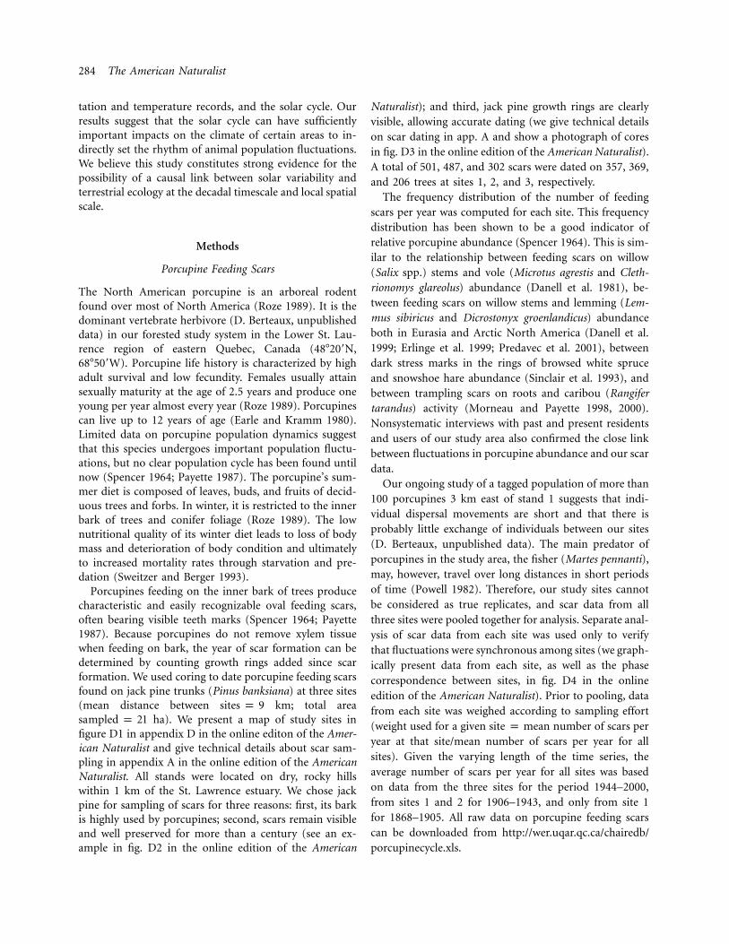
Spring temperature displayed a significant and almostcontinuous 22-year periodicity (fig. 2c, 2d), which induceda high and continuous coherence between solar irradianceand spring temperature (fig. 3a) and between spring tem-perature and porcupine scars (fig. 3f) at the 22-year pe-riodicity. In addition, phase analysis showed strong phaselocking between these three series at the 22-year periodicity(fig. 3d, 3e, 3i, 3j). As expected by the absence of 11-yearperiodicity in the spring temperature data, there was apoor phase locking between spring temperature and solarirradiance (fig. 3b, 3c) and between spring temperatureand porcupine scars (fig. 3g, 3h) at the 11-year periodicity.

Both the 11- and 22-year periodicities were present inthe winter precipitation series (fig. 2h), with the 22-yearcycle displaying greater continuity than the 11-year cycle(fig. 2g). Coherence with solar irradiance (fig. 4a) and withporcupine abundance (fig. 4f) was relatively continuous,and the phase difference between series remained relativelyconstant at both the 11- (fig. 4b, 4c, 4g, 4h) and 22-year(fig. 4d, 4e, 4i, 4j) periodicities. Only the 22-year cycle waspresent in the snowfall series (fig. 2k, 2l). This periodicity

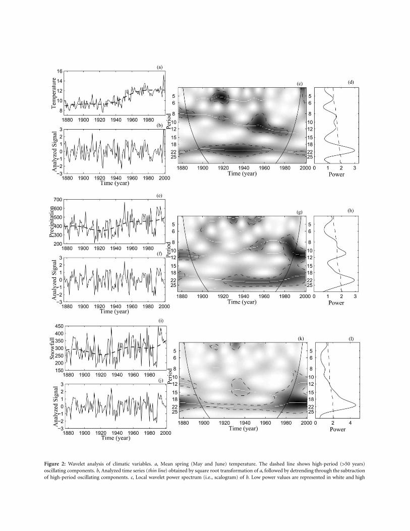
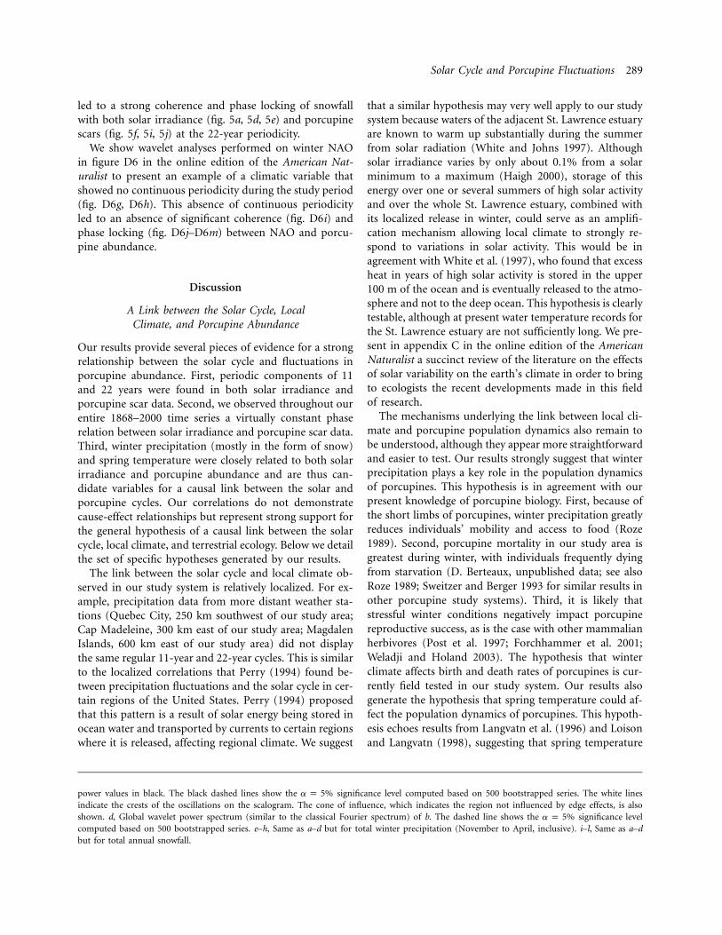
Figure 2: Wavelet analysis of climatic variables. a, Mean spring (May and June) temperature. The dashed line shows high-period (150 years)oscillating components. b, Analyzed time series (thin line) obtained by square root transformation of a, followed by detrending through the subtractionof high-period oscillating components. c, Local wavelet power spectrum (i.e., scalogram) of b. Low power values are represented in white and high


power values in black. The black dashed lines show the significance level computed based on 500 bootstrapped series. The white linesa p 5%indicate the crests of the oscillations on the scalogram. The cone of influence, which indicates the region not influenced by edge effects, is alsoshown. d, Global wavelet power spectrum (similar to the classical Fourier spectrum) of b. The dashed line shows the significance levela p 5%computed based on 500 bootstrapped series. e–h, Same as a–d but for total winter precipitation (November to April, inclusive). i–l, Same as a–dbut for total annual snowfall.

led to a strong coherence and phase locking of snowfallwith both solar irradiance (fig. 5a, 5d, 5e) and porcupinescars (fig. 5f, 5i, 5j) at the 22-year periodicity.

We show wavelet analyses performed on winter NAOin figure D6 in the online edition of the American Nat-uralist to present an example of a climatic variable thatshowed no continuous periodicity during the study period(fig. D6g, D6h). This absence of continuous periodicityled to an absence of significant coherence (fig. D6i) andphase locking (fig. D6j–D6m) between NAO and porcu-pine abundance.

Discussion

A Link between the Solar Cycle, LocalClimate, and Porcupine Abundance

Our results provide several pieces of evidence for a strongrelationship between the solar cycle and fluctuations inporcupine abundance. First, periodic components of 11and 22 years were found in both solar irradiance andporcupine scar data. Second, we observed throughout ourentire 1868–2000 time series a virtually constant phaserelation between solar irradiance and porcupine scar data.Third, winter precipitation (mostly in the form of snow)and spring temperature were closely related to both solarirradiance and porcupine abundance and are thus can-didate variables for a causal link between the solar andporcupine cycles. Our correlations do not demonstratecause-effect relationships but represent strong support forthe general hypothesis of a causal link between the solarcycle, local climate, and terrestrial ecology. Below we detailthe set of specific hypotheses generated by our results.

The link between the solar cycle and local climate ob-served in our study system is relatively localized. For ex-ample, precipitation data from more distant weather sta-tions (Quebec City, 250 km southwest of our study area;Cap Madeleine, 300 km east of our study area; MagdalenIslands, 600 km east of our study area) did not displaythe same regular 11-year and 22-year cycles. This is similarto the localized correlations that Perry (1994) found be-tween precipitation fluctuations and the solar cycle in cer-tain regions of the United States. Perry (1994) proposedthat this pattern is a result of solar energy being stored inocean water and transported by currents to certain regionswhere it is released, affecting regional climate. We suggest

that a similar hypothesis may very well apply to our studysystem because waters of the adjacent St. Lawrence estuaryare known to warm up substantially during the summerfrom solar radiation (White and Johns 1997). Althoughsolar irradiance varies by only about 0.1% from a solarminimum to a maximum (Haigh 2000), storage of thisenergy over one or several summers of high solar activityand over the whole St. Lawrence estuary, combined withits localized release in winter, could serve as an amplifi-cation mechanism allowing local climate to strongly re-spond to variations in solar activity. This would be inagreement with White et al. (1997), who found that excessheat in years of high solar activity is stored in the upper100 m of the ocean and is eventually released to the atmo-sphere and not to the deep ocean. This hypothesis is clearlytestable, although at present water temperature records forthe St. Lawrence estuary are not sufficiently long. We pre-sent in appendix C in the online edition of the AmericanNaturalist a succinct review of the literature on the effectsof solar variability on the earth’s climate in order to bringto ecologists the recent developments made in this fieldof research.

The mechanisms underlying the link between local cli-mate and porcupine population dynamics also remain tobe understood, although they appear more straightforwardand easier to test. Our results strongly suggest that winterprecipitation plays a key role in the population dynamicsof porcupines. This hypothesis is in agreement with ourpresent knowledge of porcupine biology. First, because ofthe short limbs of porcupines, winter precipitation greatlyreduces individuals’ mobility and access to food (Roze1989). Second, porcupine mortality in our study area isgreatest during winter, with individuals frequently dyingfrom starvation (D. Berteaux, unpublished data; see alsoRoze 1989; Sweitzer and Berger 1993 for similar results inother porcupine study systems). Third, it is likely thatstressful winter conditions negatively impact porcupinereproductive success, as is the case with other mammalianherbivores (Post et al. 1997; Forchhammer et al. 2001;Weladji and Holand 2003). The hypothesis that winterclimate affects birth and death rates of porcupines is cur-rently field tested in our study system. Our results alsogenerate the hypothesis that spring temperature could af-fect the population dynamics of porcupines. This hypoth-esis echoes results from Langvatn et al. (1996) and Loisonand Langvatn (1998), suggesting that spring temperature

290

Figure 3: Coherence and phase analysis of mean spring temperature in relation to solar irradiance and porcupine abundance index. a, Coherence between solar irradiance and mean springtemperature. Low power values are represented in white and high power values in black. The white dashed lines show the significance level computed based on 500 bootstrapped series.a p 5%The cone of influence, which indicates the region not influenced by edge effects, is also shown. b, Phase time series of solar irradiance (thin solid line) and spring temperature (dashed line) computedin the 10–12-year periodic band. The bold line displays the phase difference evolution. c, Distribution of phase differences; normalized entropy of the , based on 500distribution p 0.22 P 1 .1bootstrapped series. d, Same as b but computed in the 21–23 periodic band. e, Distribution of phase differences; normalized entropy of the , based on 500 bootstrappeddistribution p 0.50 P p .04series. f, Coherence between spring temperature and porcupine abundance index. g, Phase time series of spring temperature (thin solid line) and porcupine abundance index (dashed line) computedin the 10–12-year periodic band. The bold line displays the phase difference evolution. h, Distribution of phase differences; normalized entropy of the , based on 500distribution p 0.40 P p .014bootstrapped series. i, Same as g but computed in the 21–23 periodic band. j, Distribution of phase differences; normalized entropy of the , based on 500 bootstrappeddistribution p 0.66 P p .016series.

291

Figure 4: Coherence and phase analysis of total winter precipitation in relation to solar irradiance and porcupine abundance index. All symbols and values are as in figure 3. Normalized entropyof the distribution in , . Normalized entropy of the distribution in , . Normalized entropy of the distribution in , . Normalized entropy of thec p 0.41 P 1 .014 e p 0.41 P 1 .1 h p 0.36 P p .028distribution in , .j p 0.45 P 1 .1

Figure 5: Coherence and phase analysis of total annual snowfall in relation to solar irradiance and porcupine abundance index. All symbols and values as in figure 3. Normalized entropy of thedistribution in , . Normalized entropy of the distribution in , . Normalized entropy of the distribution in , . Normalized entropy of the distributionc p 0.13 P 1 .1 e p 0.58 P p .034 h p 0.24 P 1 .1in , .j p 0.60 P p .026


can have an important impact on the population dynamicsof mammalian herbivores through its impact on foragequality and survival of juveniles.

Whereas research on other mammalian herbivores sug-gests that climatic variations do have the potential to in-duce population fluctuations through persistent cohort ef-fects (Saether 1997; Post and Stenseth 1999), it wouldprobably be naive to generate the simple hypothesis thatthe solar-induced climate cycle causes the porcupine pop-ulation cycle (Stenseth et al. 2002). Rather, we hypothesizethat delayed density-dependent factors alone may be suf-ficient to generate porcupine population fluctuations butthat density-independent climatic factors may act as en-vironmental pacemakers giving the porcupine cycle its ob-served periodicity. These environmental pacemakerswould act through their recurrent perturbing influence onsurvival and reproductive success of individuals. This isanalogous to the hypothesis stating that environmentalvariation generates spatial synchrony among populationsover large geographical areas (Grenfell et al. 1998; Myers1998; Bjørnstad et al. 1999; Hudson and Cattadori 1999;Stenseth et al. 1999; Cazelles and Boudjema 2001; Cazelleset al. 2003) and in a variety of taxa (mammals, Ranta etal. 1997a; birds, Cattadori et al. 2000; insects, Liebholdand Kamata 2000; reptiles, Chaloupka 2001).

Previous data on porcupine population fluctuations inother locations, although very scarce, support the idea thatthis species undergoes fluctuations in abundance but thatthese are not necessarily periodic. Keith and Cary (1991)reported a fivefold difference between extremes in por-cupine abundance based on 11 years of capture data inAlberta, but their time series was too short to infer any-thing about the periodicity in population fluctuations.Spencer (1964) obtained 80 years of porcupine scar datain Colorado, and although he identified three peaks inporcupine abundance, these did not seem regularly spacedand were related neither to our data nor to the solar cycle.Payette (1987) used porcupine feeding scars as an indicatorof past porcupine presence along the Hudson Bay coastof Quebec but found no periodicity in his results. It there-fore appears that the periodicity of porcupine fluctuationsfound in our study system is not widespread but may existonly in certain locations in which there are strong climaticoscillations. Dendrochronological studies performed inecosystems under various climatic regimes would allowtesting of this hypothesis.

Population Cycles and the Solar Cycle Hypothesis

It is now well established that global climatic oscillations,such as the NAO and El Nino–Southern Oscillation(ENSO), can affect not only the population dynamics ofmammalian herbivores (Post et al. 1997; Lima et al. 1999;

Forchhammer et al. 2001) but also entire ecosystems (Jak-sic 2001; Ottersen et al. 2001; Blenckner and Hillebrand2002; Stenseth et al. 2002). Similarly, we hypothesize thatthe climate of certain regions (such as the area surroundingthe St. Lawrence estuary) responds particularly well todecadal variations in solar activity and that this solar-induced climatic oscillation has cascading effects on entireecosystems. Our finding of a link between the solar cycleand fluctuations in the abundance of the dominant mam-malian herbivore in a forest ecosystem may therefore bejust an example of a more global phenomenon.

At present, however, we know of only two examples ofa solar-induced climatic oscillation acting as an environ-mental pacemaker to animal population dynamics. Usingbrowsing stress marks produced in the tree rings of whitespruce (Picea glauca) by snowshoe hare (Lepus ameri-canus), Sinclair et al. (1993) reconstructed past fluctuationsin hare abundance at Kluane, Yukon. Analysis of this treering data revealed that during periods when the amplitudeof the 11-year sunspot cycle was particularly high, hareabundance did cycle in phase with the sunspot cycle, al-though it came out of phase at other times. On the basisof this evidence, as well as climatic data linked with thesunspot cycle, they suggested that the snowshoe hare cycle“is modulated indirectly by solar activity through an am-plified climate cycle that affects the whole boreal forestecosystem” (Sinclair et al. 1993, p. 195). Ranta et al.(1997b) criticized the validity of this hypothesis and arguedthat hare cycles in Finland are not synchronized with thosein North America and that the level of synchrony betweenlocal hare populations decreases with increasing distanceboth in Finland and Canada (Smith 1983). This, accordingto them, was contrary to what one would expect if anexternal factor was “setting the beat” of the hare cycle.Lindstrom et al. (1996) also rejected the possibility of asolar cycle–climate-hare-lynx causal relationship based ona time series analysis of the famous 1821–1934 MackenzieRiver lynx fur return time series and sunspot data for thesame period. Sinclair and Gosline (1997) reanalyzed thedata used by Ranta et al. (1997b) and found that althoughlocal hare populations are not always in phase across Can-ada, they do come into phase during the peak years, sug-gesting the influence of an external synchronizer such asweather acting on a continental scale. They maintainedtheir hypothesis that solar activity, when it is particularlystrong, acts indirectly as the synchronizer of the hare cyclethrough its effect on climate. They specified that becauseweather systems have different phase relations with solaractivity in different areas of the globe, we can expect thatsolar-hare phase relations will also differ (Sinclair and Gos-line 1997).

The sunspot hypothesis was also put forth to explainsynchrony and periodicity of insect outbreaks, although


again the empirical evidence was not strong enough toconclude a strong relationship (Myers 1998; Ruohomakiet al. 2000). Our results thus appear unique in that theyare the first example of a population cycle that followsboth the solar cycle and local climate fluctuations withsuch regularity and consistency over an extended periodof time (130 years).

As shown above, the possibility of a link between thesolar cycle, climate, and animal cycles has generated avigorous debate (MacLulich 1937; Elton and Nicholson1942; Moran 1949, 1953a, 1953b; Royama 1992; Lindstromet al. 1996) and is still active 80 years after it was first putforth by Elton (1924). This underscores how difficult it isto either accept or reject the hypothesis of a solar cycle,population dynamics link. This difficulty partly stems fromthe fact that very few long time series of animal populationfluctuations are available for analysis. When these ecolog-ical time series exist, their analysis is often complicated bytheir lack of linearity and stationarity (Cazelles and Stone2003). In addition, even if empirical correlations arefound, testing them with manipulative experiments is verydifficult. Finally, the influence of the solar cycle seemsdiscontinuous in time (it can disappear or even reversephases during periods of low-amplitude solar cycles) andspace (it can have different effects in different geographicalareas; Hoyt and Schatten 1997), which complicates gen-eralizations to be drawn from individual studies.

The solar cycle hypothesis raises questions about theapproach that should be used to test it. Holling and Allen(2002) recently summarized what we think is the bestavenue to progress in such complex, multisystem, andmultiscale science. They proposed that to distinguish cred-ible from incredible patterns in nature, a cycle of inquiry(called “adaptive inference”) is the most likely to lead toprogress. In this cycle, no unambiguous test can distin-guish among alternative hypotheses. Only a suite of testsof different kinds can do so, producing a body of evidencein support of one line of argument and not others. Thiscontrasts with strong inference (Platt 1964), which is basedon hypothesis falsification and where the main objectiveis to avoid Type I error. Research on both the multiyearpopulation cycles of northern mammals and the effects ofsolar variability on climate and ecosystems is likely to ben-efit from the use of adaptive inference in addition to stronginference.

Acknowledgments

We thank C. Daguerre and P. Morin for field assistanceand Parc National du Bic for providing facilities. P. Morinand two anonymous reviewers provided many helpfulcomments on the manuscript. I.K. was supported by anM.S. scholarship from the Natural Sciences and Engi-

neering Research Council of Canada (NSERC). B.C. waspartially supported by the French Ministry of Ecology andSustainable Resources, through grants Quantification desRisques d’Emergence d’Epidemies a Cholera dans le BassinMediterraneen en Relation avec le Changement Clima-tique and Modelisation des Arboviroses Tropicales Emer-gentes Climato-dependantes of the program Gestion etImpacts du Changement Climatique. Research was fundedby grants to D.B. from the NSERC, the Fonds de Recherchesur la Nature et les Technologies du Quebec, and the Can-ada Research Chair program.

Literature Cited

Bjørnstad, O. N., R. A. Ims, and X. Lambin. 1999. Spatialpopulation dynamics: analyzing patterns and processesof population synchronicity. Trends in Ecology & Evo-lution 14:427–432.

Blenckner, T., and H. Hillebrand. 2002. North AtlanticOscillation signatures in aquatic and terrestrial ecosys-tems: a meta-analysis. Global Change Biology 8:203–212.

Bond, G., B. Kromer, J. Beer, R. Muscheler, M. N. Evans,W. Showers, S. Hoffman, R. Lotti-Bond, I. Hajdas, andG. Bonani. 2001. Persistent solar influence on NorthAtlantic climate during the Holocene. Science 294:2130–2136.

Bradshaw, G. A., and T. A. Spies. 1992. Characterizingcanopy gap structure in forest using wavelet analysis.Journal of Ecology 80:205–215.

Cattadori, I. M., S. Merler, and P. J. Hudson. 2000. Search-ing for mechanisms of synchrony in spatially structuredgamebird populations. Journal of Animal Ecology 69:620–638.

Cazelles, B., and G. Boudjema. 2001. The Moran effectand phase synchronization in complex spatial com-munity dynamics. American Naturalist 157:670–676.

Cazelles, B., and L. Stone. 2003. Detection of imperfectpopulation synchrony in an uncertain world. Journal ofAnimal Ecology 72:953–968.

Cazelles, B., G. Boudjema, and L. Stone. 2003. Chaos syn-chrony induced by environmental perturbations in cha-otic populations. Pages 262–269 in V. Capasso, ed.Mathematical modelling and computing in biology andmedicine. Progetto Leonaro, Bologna.

Chaloupka, M. 2001. Historical trends, seasonality andspatial synchrony in green sea turtle egg production.Biological Conservation 101:263–279.

Chatfield, C. 1989. The analysis of time series: an intro-duction. 4th ed. Chapman & Hall, London.

Climatic Research Unit. 2001. http://www.cru.uea.ac.uk/cru/data/nao.htm.

Cook, E. R., D. M. Meko, and C. W. Stockton. 1997. A


new assessment of possible solar and lunar forcing ofthe bidecadal drought rhythm in the Western UnitedStates. Journal of Climate 10:1343–1356.

Crowley, T. J. 2000. Causes of climate change over the past1000 years. Science 289:270–277.

Currie, R. G. 1993a. Deterministic signals in European fishcatches, wine harvest, and sea-level, and further exper-iments. International Journal of Climatology 13:665–687.

———. 1993b. Luni-solar 18.6 and 10–11 year solar cyclesignals in USA air temperature records. InternationalJournal of Climatology 13:31–50.

———. 1994. Variance contribution of luni-solar and so-lar cycle signals in the St. Laurence and Nile river rec-ords. International Journal of Climatology 14:843–852.

Currie, R. G., and D. P. O’Brien. 1988. Periodic 18.6 yearand cyclic 10 to 11 year signals in north-eastern UnitedStates precipitation data. International Journal of Cli-matology 8:255–281.

———. 1990. Deterministic signals in precipitation rec-ords from the American corn belt. International Journalof Climatology 10:179–189.

Dale, M. R. T., and M. Mah. 1998. The use of waveletsfor spatial pattern analysis in ecology. Journal of Veg-etation Science 9:805–815.

Danell, K., L. Ericson, and K. Jakobsson. 1981. A methodfor describing former fluctuations of voles. Journal ofWildlife Management 45:1018–1021.

Danell, K., S. Erlinge, G. Hogstedt, D. Hasselquist, E.-B.Olofsson, T. Seldal, and M. Svensson. 1999. Trackingpast and ongoing lemming cycles on Eurasian tundra.Ambio 28:225–229.

Earle, R. D., and K. R. Kramm. 1980. Techniques for agedetermination in the Canadian porcupine. Journal ofWildlife Management 44:413–419.

Efron, B., and R. J. Tibshirani. 1993. An introduction tothe bootstrap. Chapman & Hall, New York.

Elton, C. 1924. Periodic fluctuations in the numbers ofanimals: their causes and effects. British Journal of Ex-perimental Biology 2:119–163.

Elton, C., and M. Nicholson. 1942. The ten-year cycle innumbers of the lynx in Canada. Journal of Animal Ecol-ogy 11:215–244.

Erlinge, S., K. Danell, P. Frodin, D. Hasselquist, P. Nilsson,E.-B. Olofsson, and M. Svensson. 1999. Asynchronouspopulation dynamics of Siberian lemmings across thePalaearctic tundra. Oecologia (Berlin) 119:493–500.

Forchhammer, M. C., T. H. Clutton-Brock, J. Lindstrom,and S. D. Albon. 2001. Climate and population densityinduce long-term cohort variation in a northern un-gulate. Journal of Animal Ecology 70:721–729.

Foukal, P. V. 1990. The variable sun. Scientific American262:34–41.

Friis-Christensen, E. 2000. Solar variability and climate, asummary. Space Science Reviews 94:411–421.

Friis-Christensen, E., and K. Lassen. 1991. Length of thesolar cycle: an indicator of solar activity closely asso-ciated with climate. Science 254:698–700.

Grenfell, B. T., K. Wilson, B. F. Finkenstadt, T. N. Coulson,S. Murray, S. D. Albon, J. M. Pemberton, T. H. Clutton-Brock, and M. J. Crawley. 1998. Noise and determinismin synchronized sheep dynamics. Nature 394:674–677.

Grenfell, B. T., O. N. Bjørnstad, and J. Kappey. 2001. Trav-elling waves and spatial hierarchies in measles epidem-ics. Nature 414:716–723.

Haigh, J. D. 1996. The impact of solar variability on cli-mate. Science 272:981–984.

———. 1999. Modelling the impact of solar variability onclimate. Journal of Atmospheric, Solar and TerrestrialPhysics 61:63–72.

———. 2000. Solar variability and climate. Weather 55:399–407.

———. 2001. Climate variability and the influence of theSun. Science 294:2109–2111.

Hodell, D. A., M. Brenner, J. H. Curtis, and T. Guilderson.2001. Solar forcing of drought frequency in the Mayalowlands. Science 292:1367–1370.

Holling, C. S., and C. R. Allen. 2002. Adaptive inferencefor distinguishing credible from incredible patterns innature. Ecosystems 5:319–328.

Hoyt, D. V., and K. H. Schatten. 1997. The role of the sunin climate change. Oxford University Press, New York.

Hudson, P. J., and I. M. Cattadori. 1999. The Moran effect:a cause of population synchrony. Trends in Ecology &Evolution 14:1–2.

Hurrell, J. W. 1995. Decadal trends in the North AtlanticOscillation: relationships to regional temperatures andprecipitation. Science 269:676–679.

Jaksic, F. M. 2001. Ecological effects of El Nino in terrestrialecosystems of western South America. Ecography 24:241–250.

Keith, L. B., and J. R. Cary. 1991. Mustelid, squirrel, andporcupine population trends during a snowshoe harecycle. Journal of Mammalogy 72:373–378.

Kerr, R. A. 1987. Sunspot-weather correlation found. Sci-ence 238:479–480.

———. 1988. Sunspot-weather link holding up. Science243:1124–1125.

———. 1990. Sunspot-weather link is down but not out.Science 248:684–685.

Krebs, C. J., R. Boonstra, S. Boutin, and A. R. E. Sinclair.2001. What drives the 10-year cycle of snowshoe hares?BioScience 51:25–35.

Langvatn, R., S. D. Albon, T. Burkey, and T. H. Clutton-Brock. 1996. Climate, plant phenology and variation in


age of first reproduction in a temperate herbivore. Jour-nal of Animal Ecology 65:653–670.

Lean, J. L., J. Beer, and R. Bradely. 1995. Reconstructionof solar irradiance since 1610: implications for climatechange. Geophysical Research Letters 22:3195–3198.

Liebhold, A., and N. Kamata. 2000. Are population cyclesand spacial synchrony a universal characteristic of forestinsect populations? Population Ecology 42:205–209.

Lima, M., J. E. Keymer, and F. M. Jaksic. 1999. El Nino–Southern Oscillation–driven rainfall variability and de-layed density dependence cause rodent outbreaks inwestern South America: linking demography and pop-ulation dynamics. American Naturalist 153:476–491.

Lindstrom, J., H. Kokko, and E. Ranta. 1996. There isnothing new under the sunspots. Oikos 77:565–568.

Loison, R., and R. Langvatn. 1998. Short- and long-termeffects of winter and spring weather on growth andsurvival of red deer in Norway. Oecologia (Berlin) 116:489–500.

MacLulich, D. A. 1937. Fluctuations in the numbers ofthe varying hare (Lepus americanus). University of To-ronto Studies, series no. 43. University of Toronto Press,Toronto.

Mallat, S. 1998. A wavelet tour of signal processing. Ac-ademic Press, San Diego, Calif.

Mann, M. E., R. S. Bradley, and M. K. Hughes. 1998.Global-scale temperature patterns and climate forcingover the past six centuries. Nature 392:779–787.

Meteorological Service of Canada. 2000. Canadian dailyclimate data: temperature and precipitation, Quebec.CD-ROM. Environment Canada, Downsview, Ontario.

Mitchell, J. M., C. W. Stockton, and D. M. Mekko. 1979.Evidence of a 22-year rhythm of drought in the westernUnited States related to the half solar cycle since the17th century. Pages 125–143 in B. M. McCormac andT. A. Seliga, eds. Solar terrestrial influences on weatherand climate. Reidel, Dordrecht.

Moran, P. A. P. 1949. The statistical analysis of the sunspotand lynx cycles. Journal of Animal Ecology 18:115–116.

———. 1953a. The statistical analysis of the Canadianlynx cycle. I. Structure and prediction. Australian Jour-nal of Zoology 1:163–173.

———. 1953b. The statistical analysis of the Canadianlynx cycle. II. Synchronization and meteorology. Aus-tralian Journal of Zoology 1:291–298.

Morneau, C., and S. Payette. 1998. A dendroecologicalmethod to evaluate past caribou (Rangifer tarandus L.)activity. Ecoscience 5:64–76.

———. 2000. Long-term fluctuations of a caribou pop-ulation revealed by tree-ring data. Canadian Journal ofZoology 78:1784–1790.

Mursula, K., I. G. Usoskin, and G. A. Kovaltsov. 2001.

Persistent 22-year cycle in sunspot activity: evidence fora solar magnetic field. Solar Physics 198:51–56.

Myers, J. H. 1998. Synchrony in outbreaks of forest Lep-idoptera: a possible example of the Moran effect. Ecol-ogy 79:1111–1117.

Ottersen, G., B. Planque, A. Belgrano, E. Post, P. C. Reid,and N. C. Stenseth. 2001. Ecological effects of the NorthAtlantic Oscillation. Oecologia (Berlin) 128:1–14.

Park, Y. H., and L. Gamberoni. 1995. Large-scale circu-lation and its variability in the south Indian Ocean fromTOPEX/POSEIDON altimetry. Journal of GeophysicalResearch 100:24911–24929.

Parker, K. L., C. T. Robbins, and T. A. Hanley. 1984. Energyexpenditures for locomotion by mule deer and elk. Jour-nal of Wildlife Management 48:474–488.

Payette, S. 1987. Recent porcupine expansion at the treeline: a dendrochronological analysis. Canadian Journalof Zoology 65:551–557.

Percival, D. 1995. On estimation of wavelet variance.Biometrika 82:619–631.

Perry, C. A. 1994. Solar-irradiance variations and regionalprecipitation fluctuations in the western USA. Inter-national Journal of Climatology 14:969–983.

Platt, J. R. 1964. Strong inference. Science 146:347–353.Post, E., and N. C. Stenseth. 1999. Climatic variability,

plant phenology, and northern ungulates. Ecology 80:1322–1339.

Post, E., N. C. Stenseth, R. Langvatn, and J. M. Fromentin.1997. Global climate change and phenotypic variationamong deer cohorts. Proceedings of the Royal Societyof London B 264:1317–1324.

Powell, R. A. 1982. The fisher. University of MinnesotaPress, Minneapolis.

Predavec, M., C. J. Krebs, K. Danell, and R. Hyndman.2001. Cycles and synchrony in the collared lemming(Dicrostonyx groenlandicus) in Arctic North America.Oecologia (Berlin) 126:216–224.

Ranta, E., V. Kaitala, J. Lindstrom, and E. Helle. 1997a.The Moran effect and synchrony in population dynam-ics. Oikos 78:136–142.

Ranta, E., J. Lindstrom, V. Kaitala, H. Kokko, H. Linden,and E. Helle. 1997b. Solar activity and hare dynamics:a cross-continental comparison. American Naturalist149:765–775.

Reid, G. C. 2000. Solar variability and the earth’s climate:introduction and overview. Space Science Reviews 94:1–11.

Rind, D. 2002. The sun’s role in climate variations. Science296:673–677.

Royama, T. 1992. Analytical population dynamics. Chap-man & Hall, London.

Roze, U. 1989. The North American porcupine. Smith-sonian Institution, Washington, D.C.


Ruohomaki, K., M. Tanhuanpaa, M. P. Ayres, P. Kaita-niemi, T. Tammaru, and E. Haukioja. 2000. Causes ofcyclicity of Epirrita autumnata (Lepidoptera, Geo-metridae): grandiose theory and tedious practice. Pop-ulation Ecology 42:211–223.

Saether, B. E. 1997. Environmental stochasticity and pop-ulation dynamics of large herbivores: a search for mech-anisms. Trends in Ecology & Evolution 12:143–149.

Shindell, D., D. Rind, N. Balachandran, J. Lean, and P.Lonergan. 1999. Solar cycle variability, ozone, and cli-mate. Science 284:305–308.

Sinclair, A. R. E., and J. M. Gosline. 1997. Solar activityand mammal cycles in the Northern Hemisphere. Amer-ican Naturalist 149:776–784.

Sinclair, A. R. E., J. M. Gosline, G. Holdsworth, C. J. Krebs,S. Boutin, J. N. M. Smith, R. Boonstra, and M. Dale.1993. Can the solar cycle and climate synchronize thesnowshoe hare cycle in Canada? evidence from the treerings and ice cores. American Naturalist 141:173–198.

Smith, C. H. 1983. Spacial trends in Canadian snowshoehare, Lepus americanus, populations cycles. CanadianField-Naturalist 97:151–160.

Spencer, D. A. 1964. Porcupine population fluctuations inpast centuries revealed by dendrochronology. Journal ofApplied Ecology 1:127–149.

Stenseth, N. C., K. S. Chan, H. Tong, R. Boonstra, S.Boutin, C. J. Krebs, E. Post, et al. 1999. Common dy-namic structure of Canada lynx population within threeclimatic regions. Science 285:1071–1073.

Stenseth, N. C., A. Mysterud, G. Ottersen, J. W. Hurrell,K.-S. Chan, and M. Lima. 2002. Ecological effects ofclimate fluctuations. Science 297:1292–1296.

Stockton, C. W., J. M. Mitchell, and D. M. Mekko. 1983.A reappraisal of the 22-year drought cycle. Pages 507–516 in B. M. McCormac, ed. Weather and climate re-sponses to solar variations. Colorado Associated Uni-versity Press, Boulder.

Storini, M., and J. Sykora. 1997. Coronal activity duringthe 22-year solar magnetic cycle. Solar Physics 176:417–430.

Sweitzer, R. A., and J. Berger. 1993. Seasonal dynamics ofmass and body condition in Great Basin porcupines

(Erethizon dorsatum). Journal of Mammalogy 74:198–203.

Torrence, C., and G. P. Compo. 1998. A practical guideto wavelet analysis. Bulletin of the American Meteo-rological Society 79:61–78.

Udelhofen, P. M., and R. D. Cess. 2001. Cloud cover var-iations over the United States: an influence of cosmicrays or solar variability. Geophysical Research Letters28:2617–2620.

van Loon, H., and K. Labitzke. 1988. Association betweenthe 11-year solar cycle, the QBO, and the atmosphere.II. Surface and 700 mb on the northern hemisphere inwinter. Journal of Climate 1:905–920.

———. 1998. The global range of the stratospheric de-cadal wave. I. Its association with the sunspot cycle insummer and in the annual mean, and with the tropo-sphere. Journal of Climate 11:1529–1537.

———. 2000. The influence of the 11-year solar cycle onthe stratosphere below 30 km: a review. Space ScienceReviews 94:259–278.

Vautard, R., P. Yiou, and M. Ghil. 1992. Singular spectrumanalysis: a toolkit for short, noisy chaotic signals. Phys-ica D 58:95–126.

Verschuren, D., K. R. Laird, and B. F. Cumming. 2000.Rainfall and drought in equatorial east Africa duringthe past 1,100 years. Nature 403:410–414.

Weladji, R. B., and Ø. Holand. 2003. Global climate changeand reindeer: effects of winter weather on the autumnweight and growth of calves. Oecologia (Berlin) 136:317–323.

White, L., and F. Johns. 1997. Marine environmental as-sessment of the estuary and gulf of St. Lawrence. Fish-eries and Oceans Canada, Dartmouth, Nova Scotia, andMont-Joli, Quebec.

White, W. B., J. Lean, D. R. Cayan, and M. D. Dettinger.1997. Response of global upper ocean temperature tochanging solar irradiance. Journal of Geophysical Re-search 102:3255–3266.

World Data Centre for the Sunspot Index. 2001. http://sidc.oma.be/html/sunspot.html.

Associate Editor: Rolf A. Ims

1

� 2004 by The University of Chicago. All rights reserved.

Appendix A from I. Klvana et al., “Porcupine Feeding Scars andClimatic Data Show Ecosystem Effects of the Solar Cycle”(Am. Nat., vol. 164, no. 3, p. 283)

Scar Sampling and DatingTechnical Details on Scar Sampling

Stand 1 (48�21�30�N, 68�48�30�W) had an area of 14 ha and was even aged, composed mostly of 117-year-oldjack pine, although some trees were up to 150 years old and had porcupine feeding scars up to 133 years old.Scars were sampled within 29 circular 400-m2 plots located at 25-m intervals along a transect running throughthe entire jack pine stand. Within the plots, all jack pines were inspected for presence of scars, and all scarsfound on the trunks between 0 and 1.8 m off the ground were cored ( ). Because the majority of scarsn p 575were found near ground level, it is very unlikely that sampling only between 0 and 1.8 meters off the groundintroduced a bias in our results. Of these, 501 scars located on 357 trees were dated with accuracy and used foranalysis. Stand 2 (48�20�30�N, 68�49�30�W) had an area of 5 ha and was even aged, composed mostly of 105-year-old jack pine. Because of the relative scarcity of scars, all jack pines in stand 2 were inspected, and allscars found on the trunks between 0 and 1.8 m off the ground were cored ( ). Of these, 487 scars locatedn p 519on 369 trees were dated with accuracy and used for analysis. Stand 3 (48�15�30�N, 68�59�30�W) had an area of2 ha and was also even aged, composed mostly of 77-year-old jack pine. All jack pines in the stand wereinspected, and all scars found on the trunk between 0 and 1.8 m off the ground were cored ( ). Of these,n p 373302 scars located on 206 trees were dated with accuracy and used for analysis.

Technical Details on Scar Dating

Cores were started in sound wood on the surface of a scar or at the edge of a scar and were taken across theentire diameter of the trunk. Because only live trees were sampled, the last growth ring located on the oppositeside from the scar, together with diagnostic growth ring sequences, served as reference years for dating back tothe scar. Two cores were taken per scar to ensure accurate dating. Cores were glued onto grooved plywoodboards directly in the field, air dried, and finely sanded in the laboratory. Year of scar formation was determinedunder a binocular lens by counting tree rings. Because most scars in our study sites were produced in Novemberand December (I. Klvana, unpublished data), all scars were dated as if they were produced at the end of acalendar year (November or December) in the same year as the preceding growing season. Reliability of coringas opposed to taking cross sections (Payette 1987) was verified by comparing dates obtained from cores andcross sections of 30 scars. When two or more scars of the same age were found on a given tree (5.3% of cases),only one of them was considered in a preliminary analysis. However, this decision did not affect the results, sowe included all scars in our final analyses. Some authors considered temporal changes in the availability of trees(on the basis of age distribution of trees) when reconstructing past animal activity from tree ring data (Sinclair etal. 1993; Morneau and Payette 1998, 2000). We did not do so because the trees sampled were mostly even-agedjack pine.

1


Appendix B from I. Klvana et al., “Porcupine Feeding Scars andClimatic Data Show Ecosystem Effects of the Solar Cycle”(Am. Nat., vol. 164, no. 3, p. 283)

The Wavelet AnalysisWavelets constitute a family of functions derived from a single function, the mother wavelet , which can bew(t)expressed as function of two parameters, one for the time position, t, and the other for the scale of the wavelets,a, related to the frequency. More explicitly, wavelets are defined as

1 t � tw (t) p w . (B1)a, t ( )� aa

The wavelet transform of a time series with respect to a chosen wavelet is computed as thex(t) w(a, t)convolution between the wavelet and the signal :x(t)

��

1 t � t∗ ∗W (a, t) p x(t)w dt p x(t)w (t)dt, (B2)x � � a, t( )� aa��

with an asterisk indicating the complex conjugate form. The wavelet coefficients represent theW (a, t)x

contribution of the scales, a, to the signal at different time positions, t. The computation of the wavelettransform is done along the signal (by increasing the t parameter) over a range of a scales until all thex(t)coherent structures within the signal can be identified.

In the analysis of “natural signals,” the so-called Morlet wavelet (Torrence and Compo 1998) is often applied.The Morlet wavelet is defined as

2t�1/4w(t) p p exp (�i2pf t) exp � . (B3)0 ( )2

In our study, we have used . An important point here is that a is inversely proportional to the centralf p 60

frequency of the wavelet f0. In fact, with the Morlet wavelet and the value used for f0, the frequency is equal to, or the period, p, is equal to a ( or ).1/a f p 1/a p p a

As with classical Fourier analysis using Fast Fourier Transform, the data were padded with zeros up to thenext-highest power of two (Torrence and Compo 1998). We defined the “cone of influence” to delineate a regionnear the start and the end of the series where there is a loss in statistical power and in which the values shouldbe interpreted cautiously. Nevertheless, the zero padding, owing to numerous introduced zeros, mainly induces areduction in the numerical values of the wavelet transform and their associated quantities.

In addition to the wavelet transform coefficients, we estimated the repartition of variance between a or p anddifferent t. This is known as the wavelet power spectrum, . At each time considered, the2S (p, t) p FW (p, t)Fx x

result is a three-dimensional surface or , and we presented a 2D plot (names scalogram) of theseW (a, t) S (p, t)x x

quantities against p and t parameters.We also time averaged the wavelet power spectrum to obtain a quantity analogous to the Fourier power

spectrum (called here the global wavelet power spectrum):

App. B from I. Klvana et al., “Solar Cycle and Porcupine Fluctuations”

2

T

2jx 2S (p) p W (p, t) dt, (B4)F Fx � xT0

with as the variance and T as the time duration of the time series . Percival (1995) has shown that the2j x(t)x

global wavelet power spectrum provides an unbiased and consistent estimation of the classical Fourier spectrum.To quantify statistical relationships between two time series, we used wavelet coherence (Chatfield 1989). We

computed these quantities using wavelet transform, and the wavelet coherence reads

2FAW (p, t)SFx, yR (p, t) p , (B5)x, y 2 2FAW (p, t)SF FAW (p, t)SFx y

where and indicate smoothing in both time and period, is the wavelet transform of series ,A S W (p, t) x(t)x

is the wavelet transform of , and is the cross-wavelet transform defined as∗W (p, t) y(t) W (p, t) W (p, t) py x, y x, y

. The smoothing is performed as in traditional Fourier approaches by a convolution with a∗W (p, t)W (p, t)x y

constant window function both in time and frequency directions (Chatfield 1989). The wavelet coherence,, provides local information about where two nonstationary signals, and , are linearly correlatedR (p, t) x(t) y(t)x, y

at a particular period. The coherence varies between 0 and 1. is equal to 1 when there is a perfectR (p, t)x, y

linear relation at a particular time and period between two signals.In complement to wavelet analysis, we used phase analysis to characterize and quantify the association

between signals (Cazelles and Stone 2003). The phase difference provided information on the sign of therelationship (i.e., in phase or out of phase relations). Because the Morlet wavelet is a complex wavelet, we canwrite in terms of its phase and modulus . The phase of the Morlet transform variesW (p, t) f (p, t) FW (p, t)Fx x x

cyclically between �p and p over the duration of the component waveforms and is defined as

�(W (p, t))x�1f (p, t) p tan . (B6)x �(W (p, t))x

We used resampling methods to quantify the statistical significance of the patterns exhibited by the waveletapproach (Cazelles and Stone 2003). We therefore constructed new data sets from the observed time series,which shared with the original signals some properties but were built under the null hypothesis that thevariability of the observed time series or the association between two time series is not different to that expectedby chance alone. The building of controlled data sets was performed by classical resampling methods (Efron andTibshirani 1993). We computed the wavelet transform and other estimated quantities (e.g., wavelet powerspectrum and coherence) for each bootstrapped time series, therefore generating the distribution of thesequantities under the null hypothesis. To test whether the analyzed time series were inconsistent with the nullhypothesis, we compared quantities obtained from these series with the distribution of quantities obtained frombootstrapped series. Then P values were obtained as a fraction of the control data sets giving estimated quantitiesthat were larger than those obtained from the analyzed series.

This statistical approach was also applied to the phase analyses. We quantified the phase difference betweentwo time series by the normalized entropy of their distributions (Cazelles and Stone 2003). This approachquantifies the association between the phases of two time series over the entire period, in contrast to the waveletcoherence that quantifies locally the phase association. In the case of nonstationary phase associations, the phasedifference would be nonsignificant over the entire time period.

We performed all analyses using original algorithms developed in Matlab (version 6.5, MathWorks). Theseoriginal algorithms incorporate both cross analyses and adapted statistical procedures (B. Cazelles, M. Chavez, D.Berteaux, F. Menard, J. Vik, S. Jenouvrier, and N. Stenseth, unpublished manuscript).

1


Appendix C from I. Klvana et al., “Porcupine Feeding Scars andClimatic Data Show Ecosystem Effects of the Solar Cycle”(Am. Nat., vol. 164, no. 3, p. 283)

Literature Review on the Link between the Solar Cycle and ClimateThere is growing evidence that variations in solar activity have effects on the earth’s climate at severaltimescales. However, much about these effects remains to be understood (Rind 2002). Evidence of a solaractivity–climate link appears strongest at the timescale of centuries and millennia, as suggested by both region-specific (Verschuren et al. 2000; Bond et al. 2001; Hodell et al. 2001) and planetwide studies (Mann et al. 1998;Crowley 2000). These long-term solar-related climatic oscillations have even been shown to affect humancultural development, in both Africa (Verschuren et al. 2000) and America (Hodell et al. 2001), suggesting acascading effect of variations in solar activity on entire ecosystems.

There is also much evidence of a solar activity–climate link at the timescale of the 11-year and 22-year solarcycles. The 11-year solar cycle signal was detected in various climatic and climate-related data, such as U.S.precipitation and temperature records, St. Lawrence and Nile river flows, European fish catches, wine harvests,and sea levels (Currie and O’Brien 1988, 1990; Currie 1993a, 1993b, 1994). Perry (1994) found thatprecipitation fluctuations in certain regions of the United States were highly correlated with solar activity inprevious years, while in other regions the correlation was weak or absent. This same periodicity in precipitationwas detected in net snow accumulation data from a glacier in the Yukon (Sinclair et al. 1993). Variations incloud cover over the United States were also found to be related to the solar cycle (Udelhofen and Cess 2001).The 22-year Hale solar cycle was shown to play a role in the timing and extent of drought in the United States(Mitchell et al. 1979; Stockton et al. 1983; Cook et al. 1997).

In addition to climatic responses to the solar cycle at the regional and continental scale, global planetwideresponses have also been observed. White et al. (1997) and Reid (2000) have shown that changes in solarirradiance at the scale of both the 11-year and 22-year solar cycles are reflected in the surface sea temperaturesacross the Pacific, Atlantic, and Indian Oceans. But it is perhaps the correlation found by van Loon and Labitzke(1988, 1998, 2000) between the solar cycle and the temperatures and heights of the stratosphere at 30 hPa andbelow that is the most well-known and striking evidence of a solar cycle–climate link (Kerr 1987, 1988, 1990;Haigh 2000, 2001). Modeling studies of the earth’s climate (Haigh 1996, 1999; Shindell et al. 1999) corroboratesome of the empirical evidence of a solar cycle–climate link. However, in many cases, the observed climaticresponse is much greater than what can be expected on the basis of the fact that solar irradiance varies by only0.1% from the minimum to the maximum of an 11-year cycle. This raises questions about the underlyingphysical mechanisms and suggests the existence of amplifying mechanisms (Friis-Christensen and Lassen 1991;Friis-Christensen 2000; Haigh 2000; Rind 2002). Also, the effect of the solar cycle is not felt in the same wayand with the same intensity in different regions of our planet, and our limited knowledge of our planet’s climatedoes not allow us to understand these regional discrepancies (Hoyt and Schatten 1997; Rind 2002).

1


Appendix D from I. Klvana et al., “Porcupine Feeding Scars andClimatic Data Show Ecosystem Effects of the Solar Cycle”(Am. Nat., vol. 164, no. 3, p. 283)

Online Figures

Figure D1: Map showing the location of the three jack pine stands (labeled 1, 2, and 3) in which porcupinefeeding scars were sampled.

App. D from I. Klvana et al., “Solar Cycle and Porcupine Fluctuations”

2

Figure D2: Photograph of a jack pine trunk showing a porcupine scar being cored

Figure D3: Photograph of mounted cores used for dating of porcupine feeding scars. The scar ends are on theleft side, and the live ends are on the right side. The age of a scar is obtained by subtracting the number of ringsbetween the center of the tree and the scar from the number of rings between the center of the tree and the yearof sampling.


3

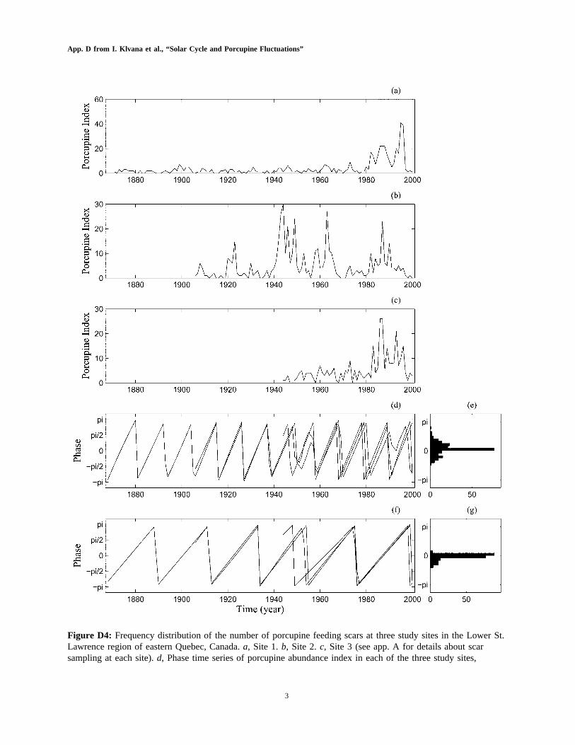
Figure D4: Frequency distribution of the number of porcupine feeding scars at three study sites in the Lower St.Lawrence region of eastern Quebec, Canada.a, Site 1.b, Site 2.c, Site 3 (see app. A for details about scarsampling at each site).d, Phase time series of porcupine abundance index in each of the three study sites,


4

computed in the 10–12-year periodic band.e, Distribution of phase differences; normalized entropy of thedistribution (pairwise , based on 500 bootstrapped series.f, g, Same asd, e, butcomparisons)p 0.38 P p .002computed in the 21–23 periodic band; normalized entropy of the distribution (pairwise ,comparisons)p 0.48

based on 500 bootstrapped series.P p .004


5

Figure D5: Wavelet analysis of porcupine abundance index and sunspot number.a, Porcupine abundance index(solid line) calculated as the pooled frequency distribution of porcupine feeding scars from three sites in easternQuebec, Canada. The dashed line shows high-period (150 years) oscillating components.b, Analyzed time series(thin line) obtained by square root transformation ofa, followed by detrending through the subtraction of high-period oscillating components. To underline the periodic components in the data, a smoothed series, obtainedusing Singular Spectrum Analysis (Vautard et al. 1992), is also shown (bold line); this last series was not used in


6

the analysis.c, Local wavelet power spectrum (i.e., scalogram) ofb. Low power values are represented in darkblue and high power values in dark red. The black dashed lines show the significance level computeda p 5%based on 500 bootstrapped series. The crests of the oscillations and the cone of influence, which indicate theregion not influenced by edge effects, are also shown on the scalogram.d, Global wavelet power spectrum(similar to the classical Fourier spectrum) ofb. The dashed line shows the significance level computeda p 5%based on 500 bootstrapped series.e, Sunspot number (solid line). The dashed line shows high-period (150 years)oscillating components.f, Analyzed time series (thin line) obtained by square root transformation ofa, followedby detrending through the subtraction of high-period oscillating components.g, Local wavelet power spectrum(i.e., scalogram) off. Interpretation similar to scalogramc. h, Global wavelet power spectrum off. The dashedline shows the significance level computed based on 500 bootstrapped series.i, Coherence betweena p 5%sunspot number and porcupine abundance index; interpretation similar to scalogramc. j, Phase time series ofsunspot number (thin solid line) and porcupine abundance index (dashed line) computed in the 10–12-yearperiodic band. The bold line displays the phase difference evolution.k, Distribution of phase differences;normalized entropy of the , based on 500 bootstrapped series.l, Same asj butdistributionp 0.45 P p .008computed in the 21–23 periodic band.m, Distribution of phase differences; normalized entropy of the

, based on 500 bootstrapped series.distributionp 0.42 P p .016


7

Figure D6: Wavelet analysis of porcupine abundance index and winter NAO index.a, Porcupine abundance


8

index (solid line) calculated as the pooled frequency distribution of porcupine feeding scars from three sites ineastern Quebec, Canada. The dashed line shows high-period (150 years) oscillating components.b, Analyzedtime series (thin line) obtained by square root transformation ofa, followed by detrending through thesubtraction of high-period oscillating components. To underline the periodic components in the data, a smoothedseries, obtained using Singular Spectrum Analysis (Vautard et al. 1992), is also shown (bold line); this last serieswas not used in the analysis.c, Local wavelet power spectrum (i.e., scalogram) ofb. Low power values arerepresented in dark blue and high power values in dark red. The black dashed lines show thea p 5%significance level computed based on 500 bootstrapped series. The crests of the oscillations and the cone ofinfluence, which indicate the region not influenced by edge effects, are also shown on the scalogram.d, Globalwavelet power spectrum (similar to the classical Fourier spectrum) ofb. The dashed line shows thea p 5%significance level computed based on 500 bootstrapped series.e, Winter NAO index (solid line). The dashed lineshows high-period (150 years) oscillating components.f, Analyzed time series (thin line) obtained by square roottransformation ofa, followed by detrending through the subtraction of high-period oscillating components.g,Local wavelet power spectrum (i.e., scalogram) off. Interpretation similar to scalogramc. h, Global waveletpower spectrum off. The dashed line shows the significance level computed based on 500 bootstrappeda p 5%series.i, Coherence between winter NAO index and porcupine abundance index; interpretation similar toscalogramsc andg. j, Phase time series of winter NAO index (thin solid line) and porcupine abundance index(dashed line) computed in the 10–12-year periodic band. The bold line displays the phase difference evolution.k,Distribution of phase differences; normalized entropy of the , based on 500distributionp 0.08 P 1 .1bootstrapped series.l, Same asj but computed in the 21–23 periodic band.m, Distribution of phase differences;normalized entropy of the , based on 500 bootstrapped series.distributionp 0.36 P 1 .1

Documents

Porcupine Feeding Scars and Climatic Data Show Ecosystem