Marshall UniversityMarshall Digital Scholar

Theses, Dissertations and Capstones

2015

Population level responses to direct applicationliming in Gyrinophilus porphyriticusShelby Renea TimmShelby_timm@hotmail.com

Follow this and additional works at: http://mds.marshall.edu/etd

Part of the Aquaculture and Fisheries Commons, and the Terrestrial and Aquatic EcologyCommons

This Thesis is brought to you for free and open access by Marshall Digital Scholar. It has been accepted for inclusion in Theses, Dissertations andCapstones by an authorized administrator of Marshall Digital Scholar. For more information, please contact zhangj@marshall.edu.

Recommended CitationTimm, Shelby Renea, "Population level responses to direct application liming in Gyrinophilus porphyriticus" (2015). Theses,Dissertations and Capstones. Paper 908.

POPULATION LEVEL RESPONSES TO DIRECT

APPLICATION LIMING IN

GYRINOPHILUS PORPHYRITICUS

Thesis submitted to

the Graduate College of

Marshall University

In partial fulfillment of the

requirements for the degree of

Master of Science

in

Biological Sciences: Organismal, Evolutionary and Ecological Biology

by

Shelby Renea Timm

Approved by

Dr. Jayme Waldron, Committee Chairperson

Dr. Thomas K. Pauley

Dr. Elmer Price

Dr. Shane Welch

Marshall University

May 2015

ii

©2015

Shelby Renea Timm

ALL RIGHTS RESERVED

iii

ACKNOWLEDGMENTS

My love for herpetology began at Kentucky Wesleyan College under the advisement of Dr. Cy

Mott, who helped me gain the necessary experience to further pursue herpetological research.

Without his direction and guidance I would not be where I am today. I would like to thank Dr.

Jayme Waldron for accepting me into her lab and for all of her help and support throughout my

graduate career at Marshall University. Her continuous encouragement and overall kind nature

made for an enjoyable and productive work environment. I have learned more than I could have

ever imagined in the past two years. Secondly, I would like to thank my committee members,

Dr. Thomas K. Pauley, Dr. Elmer Price, and Dr. Shane Welch for their continued support and

direction. Dr. Pauley always provided an open ear, whether it regarded salamander ecology or

life in general, and has been a true inspiration. It is truly an honor to have him on my committee.

Dr. Price, who spent much of his time helping me develop my skeletochronology technique and

for always reassuring me “you can’t break it” when working with the very expensive equipment

he let me use to complete my research. I thank Dr. Welch for his guidance with experimental

design and statistical analyses and for always finding new angles to consider my research from

and for challenging me. I would also like to thank the herpetology lab members, Elise Edwards,

Kelli Herrick, Derek Breakfield, Cory Goff, Jonathan Cooley, Bradley O’Hanlon, Theresa

Houze, Berlynna Heres, Matt Grisnik, and Jessyca Conatser for making graduate school a

wonderful and enjoyable experience. Thank you for all of the fun times both in and out of lab,

for all the late night “herping” and for all of our other “adventures”. I do not know what I would

have done without your support. Also, I would like to thank our honorary lab member, Oscar T.,

for bringing cuteness to the herp lab and for being a welcomed distraction from the stresses of

graduate work…even if you only like me when mom is around or if I am pushing you in your

iv

stroller. Next I want to thank my field/lab help, Elise Edwards, Thaddaeus Tuggle, Brittany

Pritt, Cory Goff, and Jessica Cantrell. I couldn’t have completed my research without you. I

want to thank my family for their unwavering support, which started long before graduate

school. From a young age you have always encouraged me to pursue my dreams and I hope that

I can continue to make you proud. Finally, none of this would have been possible without the

love and grace of God, who gave me a heart for conservation.

v

DEDICATION

I would like to dedicate this work to my mother Gwen Stevenson-Maurer for her sacrifices, for

inspiring me, and for giving me the confidence to pursue my dreams.

vi

TABLE OF CONTENTS

Acknowledgements……................................................................................................................iii

Dedication……………………………………………………………………………………...…v

Table of Contents………................................................................................................................vi

List of Tables…………………………………………………………………………………….vii

List of Figures…………………………………………………………………………………...viii

Abstract……....................................................................................................................................x

Chapter I: Population level responses to direct application liming in Gyrinophilus

porphyriticus....................................................................................................................................1

Introduction……….............................................................................................................1

Methods...............................................................................................................................6

Study Sites…...........................................................................................................6

Data Collection………............................................................................................9

Size and Age Determination……………………………………………………..11

Analysis…..............................................................................................................13

Results…............................................................................................................................16

Discussion…......................................................................................................................26

Chapter II: Gyrinophilus porphyriticus life history note……….…………………………….….33

Literature Cited..............................................................................................................................35

Appendix A....................................................................................................................................42

IACUC Approval Letter....................................................................................................48

vii

LIST OF TABLES

CHAPTER 1

1 Treatment combinations used in ANCOVAs to examine differences in body condition,

SVL, and gape size………………………………………………………………………15

2 Descriptive statistics for snout-vent length (SVL) and age for treatment and control

streams…………………………………………………………………………………...17

CHAPTER 2

1 Descriptive statistics for larval G. porphyriticus populations in the Monongahela National

Forest…………………………………………………………………………………….34

viii

LIST OF FIGURES

CHAPTER 1

1 Study site locations in the Monongahela National Forest, WV. Sites were located in

Greenbrier and Pocahontas counties………………………………………………………8

2 Sampling site locations showing paired treatment and control streams at Sugar Creek….9

3 A) Treatment stream site layout………………………………………………………….11

B) Control stream site layout…………………………………………………………….11

4 Hind limb removed from larva for skeletochronological analysis………………………13

5 A) Larva collected at the beginning of the sampling season, with a LAG located along

the peripheral edge of the bone……………..……………………………………………16

B) Larva collected at the end of the sampling season with growth behind the final

LAG…………………………………………………………………………………......16

6 Average age in years and standard deviation for control (gray) and treatment (black)

streams…………………………………………………………………………………...17

7 Average pH and standard deviation for control (gray) and treatment (black) streams….18

8 Age frequency distributions for 3-6 year larvae………………………………………...19

9 Body condition ANCOVA for treatment stream. Includes downstream site one (DS1;

red), which is located 50 m below the lime application, and the treatment reference

(blue), which is located 100 m upstream of the lime application………………………..20

10 Treatment stream ANCOVA for snout-vent-length. Includes downstream site one (DS1;

red), which is located 50 m below the lime application, and the treatment reference

(blue), which is located 100 m upstream of the lime application………………………..21

11 Control stream ANCOVA for snout-vent-length squared. Includes downstream control

site one (DSC1; red), which is located 50 m below the reference point, and the upstream

control site (blue), which is located 100 m upstream of the reference point…………….22

12 Treatment stream ANCOVA for snout-vent-length. Includes downstream site two (DS2;

red), which is located 500 m below the lime application, and the treatment reference

(blue), which is located 100 m upstream of the lime application………………………..22

ix

13 Control stream ANCOVA for snout-vent-length squared. Includes downstream control

site two (DSC2; red), which is located 500 m below the reference point, and the upstream

control site (blue), which is located 100 m upstream of the reference point…………….23

14 Treatment stream ANCOVA for gape size squared. Includes treatment reference (blue),

which is located 100 m upstream of DAL, and the first downstream treatment site (DS1;

red), which is located 50 m downstream of DAL……………………………………….24

15 Treatment stream ANCOVA for gape size. Includes treatment reference (blue), which is

located 100 m upstream of DAL, and the second downstream treatment site (DS2; red),

which is located 500 m downstream of DAL……………………………………………24

16 Control stream ANCOVA for gape size. Includes upstream control (UPC; blue), which is

located 100 m upstream of the reference point, and the first downstream control site

(DSC1; red), which is located 50 m downstream of the reference point………………...25

17 Control stream ANCOVA for gape size. Includes upstream control (UPC; blue), which is

located 100 m upstream of the reference point, and the second downstream control site

(DSC2; red), which is located 500 m downstream of the reference point……………….25

18 Direct application lime site in Dogway Fork…………………………………………….30

19 Control stream site with numerous moss covered rocks providing good habitat for

larvae……………………………………………………………………………………..31

20 Photos from DS1 site on Bear Run showing grayish precipitate………………………...31

CHAPTER 2

1 Linear correlation for SVL with age, including 95% confidence intervals……………...34

APPENDIX

1 Cross section. Zero LAGs………………………………………………………………..42

2 Cross section. One LAG…………………………………………………………………42

3 Cross section. Two LAGs………………………………………………………………..43

4 Cross section. Three LAGs………………………………………………………………44

5 Cross section. Four LAGs………………………………………………………………..45

6 Cross section. Five LAGs………………………………………………………………..46

7 Cross section. Six LAGs…………………………………………………………………47

x

ABSTRACT

Direct application liming (DAL) has been used to neutralize acidified streams to restore aquatic

biota. This mitigation technique has been used globally for decades, yet little data exist on its

effects on amphibian populations. My study investigated the effects of liming on amphibians by

measuring variability in life histories of larval Gyrinophilus porphyriticus. I collected larvae

from six streams in the Monongahela National Forest, West Virginia. I examined the effects of

DAL on age structure, and I failed to detect a treatment effect. I used ANCOVAs to examine

differences in body condition, body size, and gape size. I observed that larvae located directly

below DAL reached significantly larger body sizes at younger ages and appeared to have higher

body conditions. Larvae below DAL had significantly smaller gape sizes than larvae in the

treatment reference. By identifying the impacts of DAL on amphibian life history strategies,

biologists can better manage aquatic habitats.

1

CHAPTER 1

POPULATION LEVEL RESPONSES TO DIRECT APPLICATION LIMING IN

GYRINOPHILUS PORPHYRITICUS

INTRODUCTION

Anthropogenic stream acidification, from industrial SO2 emissions or acid mine drainage,

is a global concern due to the negative impacts it has on aquatic ecosystems (Driscoll et al.

2003). To mitigate acidification, liming, that is, the addition of calcium carbonate into aquatic

systems, has been used in many industrialized nations to neutralize pH levels and improve water

chemistry, with a majority of attention on game fisheries restoration (Eggleton et al. 1996; Mckie

et al. 2006). Multiple liming methods have been used to mitigate acidic conditions, including

dosers, full catchment, and direct application liming (Menendez et al. 1996; Menendez et al.

2000; Clair & Hindar 2005). Although liming has successfully increased pH and improved

overall water chemistry (Clayton et al. 1998; Menendez et al. 1996; Clair & Hindar 2005), the

mitigation practice itself acts as an ecological perturbation and could have broad ecological

impacts and unexpected emergent effects.

Emergent effects are often scale dependent and arise when simple mechanisms interact at

broad spatial scales (Harfoot et al. 2014) and can result when there are alterations to community

structure (Carey & Wahl 2010; Reynolds & Elliott 2012). Fine sediments associated with liming

can fill interstitial spaces within the stream, changing the physical structure of the stream

substrate and likely stressing biota (Keener & Sharpe 2005). Liming also has the potential to

alter trophic structure by changing species and predator composition, which may result in shifts

in optimal life history strategies for biota. The interaction of these changes may produce

unexpected emergent effects (Carey & Wahl 2010; Reynolds & Elliott 2012). These unexpected

consequences, such as alterations in habitat and trophic structure, are important considerations

2

given that economies of scale often encourage large-scale mitigation practices, such as liming

(Carey & Wahl 2010; Reynolds & Elliott 2012).

Previous research has demonstrated that liming can have mixed effects on stream biota,

particularly directly downstream of lime application, although results vary by stream (Clayton &

Menendez 1996; LeFevre & Sharpe 2002; Clair & Hindar 2005; Keener & Sharpe 2005;

McClurg et al. 2007). In general, liming increases fish abundance and survival and increases the

presence of acid-sensitive macroinvertebrates (Clair & Hindar 2005; Mant el al. 2013); however,

numerous studies have observed a decrease in overall macroinvertebrate abundance and diversity

below lime application sites, which was often the direct result of increased sedimentation

(LeFevre & Sharpe 2002; Keener & Sharpe 2005; Simmons et al. 2006; McClurg et al. 2007).

Macroinvertebrate and amphibian abundance can also be negatively affected by non-native trout

introduction (Finlay & Vredenburg 2007; Hartel et al. 2007), which often follows lime

application because reestablishing game fisheries is one of the primary goals of this mitigation

(Downey et al. 1994). Such variation in population-level responses to direct and indirect effects

of liming indicates the need for further investigation on the possible impacts of this mitigation

practice on aquatic biota. It is prudent to examine the utility of this mitigation practice with

emergent effects in mind to ensure that there are no unintentional negative impacts on non-target

wildlife. Specifically, there is a lack of information on how liming affects amphibians, which is

necessary to understand broader impacts, such as ecological integrity (Welsh & Droege 2001).

Amphibians are considered indicators of ecosystem health and integrity (Corn & Bury

1989; Welsh & Olliver 1998; Welsh & Droege 2001). Sedimentation is a major perturbation in

many streams, leading to the loss of microhabitat (Waters 1995), and has been shown to

negatively affect stream salamander abundance and survival (Welsh & Olliver 1998; Bonin

3

1999; Lowe & Bolger 2002). In addition to their sensitivity to sedimentation, salamander larvae

have permeable skin, limited dispersal, and cannot escape aquatic conditions until

metamorphosis, which make them good models for my study (Petranka 1998; Lowe 2003).

Specifically, Gyrinophilus porphyriticus, the Spring Salamander, is an ideal study species due to

its highly plastic life history with an aquatic larval stage ranging from three to six years, which

varies depending on a number of environmental conditions (Bruce 1980; Resetarits 1995).

Gyrinophilus porphyriticus is an appropriate biological indicator because it relies on interstitial

habitats, which can be greatly reduced below lime application sites (Bishop 1941; Bruce 1980;

Keener & Sharpe 2005). In its larval stage, G. porphyriticus serves as a gape-limited,

intermediate-to-apex predator in aquatic systems and can operate as a bellweather to trophic

perturbations (Bruce 1980; Maret & Collins 1996; Welsh & Ollivier 1998).

Phenotypic divergence is typically low in G. porphyriticus from populations in close

proximity along the stream corridor, compared to populations separated by equivalent distances

over land (Lowe et al. 2012); therefore, if environmental and trophic conditions are similar

throughout the stream, life history strategies should not differ. The reaction norm, which is the

ability of an organism’s genetics to exhibit different phenotypes in a range of environments,

reflects tradeoffs and is maintained when a species is exposed to a variety of environmental

conditions throughout its geographic range and several potential life history traits are more

beneficial than producing only a single, canalized trait (Stearns 1989; DeWitt et al. 1998;

Ghalambor et al. 2007). In G. porphyriticus, phenotypic divergence can be induced in novel or

stressful environments and apparent shifts in life history strategies can be quantified to detect

environmental changes, such that could be manifested after liming (Stearns 1992; DeWitt et al.

1998). Plasticity is adaptive when it increases fitness, neutral if there is no effect with respect to

4

fitness, or maladaptive if environmental information is unreliable/rapidly changing or if the level

of plasticity needed for a particular environment cannot overcome physiological or genetic

constraints, leading to decreased fitness (Smith-Gill 1983; DeWitt et al. 1998; Ghalambor et al.

2007). Life history shifts are often associated with tradeoffs (Hereford 2009), which reflect

constraints on resources, such that an increase in one trait necessitates a decrease in another

(Pease & Bull 1988). Tradeoffs occur when shifts in resource allocations are necessary to better

fit local environments (Luquet et al. 2015). Major tradeoffs that are common in amphibians are

variations in activity level, mortality, and growth rate and variations in size and timing of

metamorphosis (Berven & Gill 1983; Stearns 1992; Werner and Anholt 1993; Roff 2000). For

example, amphibian fitness is often positively correlated with body size, which is affected by

larval period, growth rates, and gape size (Forsman 1994). Individuals with rapid growth often

mature or complete metamorphosis earlier than individuals that have a longer larval period with

slower growth. Rapid growth is often selected for when environmental conditions are stressful or

unstable and greater fitness is achieved by maturing and reproducing at younger ages. Slower

growth, and therefore longer larval periods, occurs in stable environments and results in larger,

higher fecundity adults with increased fitness. However, a tradeoff for rapid growth may

contribute to higher mortality due to the need for increased activity levels, whereas a tradeoff for

slower growth would be forgoing reproduction until later in life (Stearns 1992; Arendt 1997).

Tradeoffs may also be caused by physical or physiological limitations from increased stress after

an environmental perturbation (Smith-Gill 1983). Therefore, optimal life history strategies vary

in different environments; however, optimal strategies under stressors from environmental

perturbations, such as liming, may not be equivalent with respect to fitness (Welsh & Olliver

1998; Teplitsky et al. 2007).

5

Direct application liming (DAL) is the instream bulk application of sand-sized limestone

and has become a widely-used method (Downey et al. 1994; Keener & Sharpe 2005) for

increasing stream pH. It is the primary method used in West Virginia and throughout

Appalachia due to its affordability, ease, and its effectiveness compared to other methods

(Ivahnenko et. al 1988; Clayton et al. 1998). Stream flow continuously distributes limestone

particles downstream until the limestone pile is eroded away, at which time more lime is added

(2-3 times per year). Limestone dissolution rates vary depending on particle size and initial pH

(Sverdrup 1986; Menendez et al. 2000). Undissolved particles can embed the natural substrate,

reducing the hyporheic zone, which is the primary habitat for many biota, including salamander

larvae (Ivahnenko et. al 1988; Waters 1995; Lowe & Bolger 2002). Reduction of microhabitat

from sedimentation can increase stress in larvae and limit predator avoidance, potentially leading

to life history shifts (Welsh & Ollivier 1998; Resetarits 1995).

Little data exist on the effects of liming on amphibian populations; therefore, my study

will examine variations in size and age of G. porphyriticus from limed and un-limed streams.

Direct application liming has the potential to either promote longer larval periods due to

improved conditions and decreased stress levels, or could lead to selection for early

metamorphosis if stress levels increase, shifting optimal life history strategies (Stearns 1992;

Arendt 1997). I used active DAL streams and un-limed control streams to examine the effects of

liming on larval G. porphyriticus life history strategies, specifically population age structure, and

individual body condition, growth, and gape size. I hypothesized that I would detect a tradeoff

between life history parameters resulting from increased sedimentation from DAL. Specifically,

I expected larvae downstream of the DAL sites to have younger populations, indicating selection

for earlier metamorphosis, and smaller individual body conditions, body size, and gape size from

6

increased stress and alterations in trophic structure. By identifying the impacts of liming on

amphibians, biologists can better manage aquatic habitats and determine if liming is beneficial to

overall stream diversity. Understanding how liming affects non-target species will aid with

improvements to methodology or bring into question the efficacy of this mitigation practice to

achieve conservation and management objectives. My research will promote future

comprehensive studies on various mitigation practices in efforts to reduce unexpected emergent

effects.

METHODS

Study Sites

I collected G. porphyriticus larvae from multiple populations in the Gauley River

watershed in Pocahontas and Greenbrier counties, near Richwood, WV, which is in the southern

portion of the Monongahela National Forest. I sampled six first- and second-order streams,

which included three treatment streams and three control streams (Figure 1). I sampled Sugar

Creek of the Williams River (treatment stream; first-order) and its neighboring unnamed

tributary (control stream; first-order), Bear Run of the North Fork Cherry River (treatment

stream; first-order) and its neighboring unnamed tributary (control stream; first-order), and

Dogway Fork of the Cranberry River (Figure 1; treatment stream; second-order) and its

neighboring unnamed tributary (control stream; first-order). Because DAL relies on a road-

crossing to apply lime fines, I selected three treatment streams and three control streams that

included an unpaved road-crossing. Streams were characterized by rocky substrates, shallow

stream depth (<1 m), and forested riparian zones. Direct application liming was applied to

treatment streams several times yearly using dump trucks. Each lime application was applied by

the West Virginia Division of Natural Resources directly into the stream to mitigate for acid

7

precipitation. The rate and volume of liming applications varied among sites. Sugar Creek was

treated twice yearly in the spring and fall, totaling 45 metric tons of limestone fines. Bear Run

was treated three times yearly in the spring, summer, and fall with a target limestone fines of 66

metric tons and Dogway Fork is limed throughout the spring, summer, and fall with nearly 250

metric tons of limestone fines. The rates and amount of application were dependent on drainage

size and original pH and was designed to bring each stream up to a neutral pH. The West

Virginia Division of Natural Resources used limestone fines that were 90% calcium carbonate or

higher. Control streams were not treated with lime and had similar stream characteristics as

treatment streams. Each treatment stream had a paired control stream to control for intra-study

variability and to increase power to detect treatment effects (Sokal & Rohlf 1981; Figure 2). Of

the available limed streams in the area, I selected streams that included large G. porphyriticus

populations, had a paired control stream, and had a sufficiently long stream channel (~0.8 km) to

incorporate three independent sampling sites.

8

Figure 1: Study site locations in the Monongahela National Forest, WV. Sites were located in

Greenbrier and Pocahontas counties.

9

Figure 2: Sampling site locations showing paired treatment and control streams at Sugar Creek.

Each stream had three sites. The control stream sites were measured from the “Reference Point”

with one site 100 m upstream (UPC) of the reference point and two sites downstream. The first

site below the reference point is 50 m downstream (DSC1) and the other site is 500 m

downstream (DSC2). Sites in the treatment stream were measured from the direct application

lime site (DAL) with one site 100 m upstream (Treatment Reference) and two sites downstream.

The first site below DAL was 50 m downstream (DS1) and the other site was 500 m downstream

(DS2).

Data Collection

Within each stream, I collected G. porphyriticus larvae from three independent locations relative

to a road crossing (N=18 sites). Sample locations within treatment streams included a treatment

reference located 100 m upstream of the DAL application site (i.e., road crossing; Figure 3A).

The first treatment site was located 50 m downstream of the DAL site (DS1) and the second

10

treatment site was located 500 m downstream of the DAL site (DS2). Control streams were

designed with the same site layout, but because there was no DAL site, the control sites were

measured from a reference point located at the road-crossing to mirror road-crossings in

treatment streams (Figure 3B). Control streams had one site located 100 m upstream of the

reference point (UPC) and two sites located downstream of the reference point at 50 m below

(DSC1) and 500 m below (DSC2). For treatment and control streams, each sampling site was

50 m long and at least 100 m from any other collection site to maintain independent larval

populations (Lowe 2003). I collected larvae on multiple sampling occasions from April 25, 2014

to August 23, 2014 until at least eight individuals were collected from each site. I selected a

sample size of 8-12 individuals per site to increase statistical power, while not overharvesting

from a single population. I collected larvae using a flip and search method during diurnal

surveys (Lowe & Bolger 2002). All cover objects were flipped throughout the site until eight

individuals were captured. Gyrinophilus porphyriticus larvae were most often found in the

interstitial spaces under cobble sized rocks (between 64 mm and 256 mm diameter; Lane 1947)

that were not embedded in the substrate and were generally located in riffles or pools (Lowe

2005). After I collected larvae, they were euthanized in MS-222 and transferred to 70% ethyl

alcohol. I recorded pH on each sampling occasion, and fish and crayfish presence. The pH of

each site was measured on at least two occasions with a pHTest ® Series, pH Testr30 meter,

measured to the nearest tenth.

11

A) Treatment stream site layout

B) Control stream site layout

Figure 3: A) Treatment stream site layout. Sites relative to the direct application lime site

(DAL). DS1= first downstream site; DS2= second downstream site. The treatment reference site

was located 100 m above lime application and was not impacted by lime. Downstream site 1

(DS1) was located 50 m below the DAL site and DS2 was located 500 m below the DAL site.

Each site was 50 m in length. B) Control stream site layout. Sites relative to random reference

point. UPC=upstream control site; DSC1= first downstream control site; DSC2= second

downstream control site. Upstream control site (UPC) was located 100 m above the reference

point. Downstream control site 1 (DSC1) was located 50 m below the reference point and DSC2

was located 500 m below the reference point. Each site was 50 m in length.

Size and Age Determination

I measured snout-vent length (SVL) of preserved larvae using calipers to the nearest 0.05

mm from the snout to the posterior edge of the cloacal slit. Wet mass was measured using a

digital scale to the nearest milligram. Body condition was calculated using a ratio index of body

mass divided by SVL so that the values could be compared across populations (Jakob et al.

1996). Gape size was measured for each larva using calipers to the nearest 0.05 mm. Gape was

measured across the width of the head from the edges of the mouth (Ohdachi 1994).

I used skeletochronological analysis of femurs for larval age determination. Age can be

determined in amphibians by counting the number of lines of arrested growth (LAGs) in the

50m

mmm DSC1 (50m)

DSC2 (500m)

UPC (100m)

Reference Point

Downstream 50m

mmm

50m

mmm

50m

mmm

Downstream Lime

Treatment Reference

DS1 (50m)

DS2 (500m)

50m

mmm

50m

mmm

50m

mmm

100m

mmm

400m

mmm

50m

mmm

DAL

12

cross-sections of the diaphysis of long bones or phalanges (Castanet et al. 1993; Smirina 1994).

Lines of arrested growth are deposited annually in temperate regions during winter when growth

slows and individuals are less active. The areas of bone between LAGs are laid during periods

of active osteogenesis and are distinguishable from the darker staining LAGs (Castanet et al.

1993). Because LAGs are generally laid annually during the winter, they provide a reliable

means of determining age (Castanet et al. 1993; Smirina 1994). This method has been verified

using amphibians of known age and is most reliable in young, rapidly growing individuals, such

as larvae (Smirina 1994). Age estimation in older individuals can be less accurate because early

LAGs can be resorbed and slowed growth rates after sexual maturity result in LAGs that are very

close together and difficult to distinguish. Thus, in this study, I limited my analysis to larval G.

porphyriticus (Smirina 1994).

After preservation, the right hind limb of each individual was removed and placed

directly into 5% nitric acid for decalcification (Bruce & Castanet 2006). Typically, the femur is

separated from the surrounding tissue and muscle before it is placed into nitric acid (Leclair &

Castanet 1987; Socha & Ogielska 2010; Ashkavandi et al. 2012); however, after trying both

methods, removing the tissue was deemed unnecessary (Figure 4). Leaving the surrounding

tissue intact made the bones easier to handle and prevented them from being damaged during

processing. Bones were decalcified for three hours then rinsed three times in deionised water

and placed in 30% sucrose. If bones were not immediately cut, they were refrigerated at 4°C.

To prepare the bone for cross-sectioning, I placed the leg upright in Tissue-Tek OCT Compound

freezing medium. I then made 15 um cross-sections (Bruce & Castanet 2006) using a Leica CM

1950 cryostat (freezing microtome) at -15° C. I placed cross-sections from the diaphysis of the

femur directly onto Superfrost Plus microscope slides (Wake & Castanet 1995; Bruce &

13

Castanet 2006; Socha & Ogielska 2010). The slides were stained in Ehrlich’s Hematoxylin for

10 minutes and then rinsed in deionised water for five minutes and permanently mounted with

Clear-Mount, an aqueous mounting medium. Ehrlich’s Hematoxylin was used because LAGs are

highly chromophilic with hematoxylin dyes (Castanet et al. 1993). Once stained, I examined the

slides under a light microscope and counted the number of LAGs for each individual. Because

each LAG was laid annually (Castanet et al. 1993; Smirina 1994), LAGs were translated directly

to age. Larvae that lacked LAGs were considered young of the year and were assigned to the

zero age class. If the sections were unclear the other femur was used to determine age.

Figure 4: Hind limb removed from larva for skeletochronological analysis. Cross-sections from

the diaphysis of the femur (circled) were used for age determination.

Analysis

I determined each individual’s age and did not have to exclude any individuals from

analysis due to unclear LAGs or regenerated limbs. I aged each individual on three separate

occasions using blind analysis to prevent bias (Castanet et al. 1993). In the event that more than

14

one age was estimated for an individual, I retained the most recurring age for analysis. Any age

discrepancies for an individual were within one year of other estimates, and no individual was

estimated to be three different ages; therefore individual age estimates were consistent.

All statistical analyses were performed in SAS® [9.4] (Copyright © 2013). I used an

ANOVA to compare variations in pH across sampling sites in both treatment and control

streams. I used Fisher’s exact tests to examine whether age frequency distributions differed

among sites and stream (i.e., DAL treatment). Because young individuals (0-2) were

underrepresented in my sample due to their secretive nature and greater use of interstitial spaces

(Resetarits 1995), and because my goal was to examine differences in metamorphic age (Bishop

1941; Bruce 1980), I excluded age classes 0-2 in the age structure analysis. I used analysis of

covariance (ANCOVA) to examine differences in body condition (dependent variables) in

treatment and control stream sites (independent variables), while controlling for variation caused

by age (covariate). I also used ANCOVAs to examine differences in SVL (dependent variable)

in treatment and control stream sites (independent variables), while controlling variation caused

by age (covariate). Differences in gape size (dependent variable) in treatment and control stream

sites (independent variables), while controlling for variation cause by SVL (covariate), were also

tested using ANCOVAs. I ran each ANCOVA with only two factors (i.e., treatment) to increase

power because my sample size was small (McDonald 2014). I tested for homogeneity of slopes

(α = 0.05) prior to running each ANCOVA. If slopes were homogenous, then the interaction

statement was removed from the final ANCOVA (Engqvist 2005). If slopes were

heterogeneous, then further analyses were not conducted. Significant covariates (α = 0.05) were

determined using Type III of sum of squares. I used ANCOVAs to test for differences in body

condition within treatment stream sites and within control stream sites (Table 1). I also used

15

ANCOVA to examine differences in SVL within treatment stream sites and within control

stream sites (Table 1). Snout-vent lengths from control streams were squared to meet the

normality assumption. I used the body size ANCOVAs as a proxy for larval growth rate,

because the analysis showed the increase in size relative to age. I analyzed gape size with

ANCOVAs to test for differences within treatment stream sites and within control stream sites

(Table 1).

Table 1: Treatment combinations used in ANCOVAs to examine differences in body condition,

SVL, and gape size. TR=Treatment Reference (100 m above DAL); DS1=first downstream

treatment (50 m below); DS2= second downstream treatment (500 m below); UPC=upstream

control (100 m above); DSC1= first downstream control (50 m below); DSC2= second

downstream control (500 m below).

ANCOVAs

Treatment Streams Control Streams

Body Condition TR vs. DS1 UPC vs. DSC1

TR vs. DS2 UPC vs. DSC2

SVL TR vs. DS1 UPC vs. DSC1

TR vs. DS2 UPC vs. DSC2

Gape Size TR vs. DS1 UPC vs. DSC1

TR vs. DS2 UPC vs. DSC2

I mirrored the distribution of sample sites within control streams to those in the treatment

streams. Although redundant, my analysis depended heavily on multiple ANCOVAs and this

approach allowed me to use comparisons among sampled sites to test specific hypotheses and

control for potential longitudinal effects (Table 1). For example, by comparing treatment

reference to DS1, I examined direct effects of DAL. By examining treatment reference to DS2, I

assessed the effects of distance from DAL. Similar analyses were performed on the control

stream with the expectation that I would not detect longitudinal differences and thus provide

further support for treatment effects. Sites from control streams were not tested against sites in

treatment streams due to fact that G. porphyriticus populations from different streams inherently

16

have greater phenotypic divergence, because dispersal is typically along the stream corridor and

not over land, meaning that there is decreased gene flow between streams (Lowe et al. 2012).

RESULTS

I collected 158 G. porphyriticus larvae. Individuals that were collected at the beginning

of the sampling season had LAGs located at the periphery of the bone section (Figure 5A),

whereas larvae collected later in the summer had growth behind the most recent LAG, so the

LAG was not at the periphery of the bone (Figure 5B). Larvae ranged from zero (young of the

year) to six years in treatment and control streams; however, I failed to detect 6-year individuals

below DAL sites (Table 2). Average age was lowest at the DS1 site (Table 2; Figure 6). Younger

age classes (0-2) were rarely encountered during sampling, likely because younger larvae inhabit

interstitial spaces, the areas between substrate particles, and are more secretive (Resetarits 1995).

A) B)

Figure 5: A) Larva collected at the beginning of the sampling season, with a LAG located along

the peripheral edge of the bone. B) Larva collected at the end of the sampling season with growth

behind the final LAG.

HL

1

2

HL

4 3 2

1

17

Table 2: Descriptive statistics for snout-vent length (SVL) and age for treatment and control

streams. Treatment sites include the treatment reference located upstream of lime application, the

first downstream site (DS1), and the second downstream site (DS2). Control sites include

upstream control site (UPC) located above the reference point, the first downstream control site

(DSC1), and the second downstream control site (DSC2). The range and mean for SVL ±

standard deviation, and the range and mean age ± standard deviation was calculated for each

sample (n).

SVL (mm) Age (years)

Treatment n Range Mean ± SD Range Mean ± SD

Treatment Reference 27 26.50-61.67 47.13 ± 9.25 0-6 3.56 ± 1.22

DS1 27 25.70-67.20 47.85 ± 12.16 0-5 2.96 ± 1.37

DS2 26 28.10-67.75 49.08 ± 10.41 1-5 3.27 ± 1.00

Control n Range Mean ± SD Range Mean ± SD

UPC 24 31.05-59.85 47.23 ± 8.08 1-6 3.25 ± 1.03

DSC1 27 35.20-58.75 48.83 ± 7.00 2-6 3.67 ± 1.21

DSC2 27 29.30-59.00 48.40 ± 7.11 1-5 3.70 ± 1.02

Figure 6: Average age in years and standard deviation for control (gray) and treatment (black)

streams. Treatment sites include the treatment reference located upstream of lime application,

the first downstream site (DS1), and the second downstream site (DS2). Control sites include

upstream control site (UPC) located above the reference point, the first downstream control site

(DSC1), and the second downstream control site (DSC2).

0

1

2

3

4

5

UPC DSC1 DSC2 Treatment

Reference

DS1 DS2

Av

era

ge

Ag

e

18

I detected a difference in pH between treatment and control streams, with a significantly

higher pH below the DAL site (F5,12 = 8.30; p = 0.001; Figure 7). The average pH in control

streams and in the treatment reference was 4.8 and the average pH below lime was 7.0.

Figure 7: Average pH and standard deviation for control (gray) and treatment (black) streams.

UPC=upstream control (100 m above); DSC1= first downstream control (50 m below); DSC2=

second downstream control (500 m below). Treatment reference is located 100m above lime

application. DS1=first downstream treatment (50 m below); DS2= second downstream treatment

(500 m below). “B” indicates that pH is significantly different than “A” (ANOVA).

I failed to detect a significant shift in age structure between sites in treatment (p = 0.35)

and control streams (p = 0.20) using the Fisher’s exact test (Figure 8). Although I failed to detect

a significant treatment effect on age structure, the predominant age class for larvae below the

DAL site was three years (57.1% in the DS1 and 63.6% in the DS2; Figure 8A) compared to

larvae in the treatment reference, which were predominantly four years old (52.2%; Figure 8B).

0

1

2

3

4

5

6

7

8

100 Control 50 Control 500 Control 100 Lime 50 Lime 500 Lime

pH

UPC DSC1 DSC2 Treatment DS1 DS2

Reference

A A A

B B

A

Control Treatment

19

A) Treatment Streams

B) Control Streams

Figure 8: Age frequency distributions for 3-6 year larvae. I failed to detect a difference in

treatment or control stream age structures. Treatment sites include the treatment reference

located upstream of lime application, the first downstream site (DS1), and the second

downstream site (DS2). Control sites include upstream control site (UPC) located above the

reference point, the first downstream control site (DSC1), and the second downstream control

site (DSC2).

0

2

4

6

8

10

12

14

16

3 4 5 6

Fre

qu

ency

Age

Treatment Reference

0

2

4

6

8

10

12

14

3 4 5 6

Fre

qu

ency

Age

DS2

DS1

DSC2

DSC1

UPC

20

I failed to detect significant differences in larval body condition between sites in

treatment and control streams. However, the analysis for the treatment reference and DS1

approached significance (F1,51 = 3.31; p = 0.07; Figure 9). Larvae from DS1 in treatment streams

appeared to reach higher body conditions than larvae in the treatment reference, compared to

control stream larvae from UPC and DSC1, which did not differ (F1,48 = 0.32; p = 0.58). I also

failed to detect a longitudinal effect in body conditions between the treatment reference and DS2

sites (F1,49 = 2.04; p = 0.16) and between the UPC and DSC2 sites (F1,48 = 0.61; p = 0.44).

Figure 9: Body condition ANCOVA for treatment stream. Includes downstream site one (DS1;

red), which is located 50 m below the lime application, and the treatment reference (blue), which

is located 100 m upstream of the lime application.

I detected a significant treatment effect on body size. Specifically, body size differed

between the treatment reference and DS1 (ANCOVA; F1,51 = 5.75; p = 0.02; Figure 10). Larvae

from DS1 in treatment streams reached larger body sizes (SVL) at younger ages than individuals

that were located above the DAL site in the treatment reference. In the ANCOVA analysis for

UPC and DSC1 in the control streams, I failed to detect a difference in body size (F1,48 = 0.03;

21

p = 0.86; Figure 11). In the treatment streams, larval body size from DS2 did not significantly

differ from larvae in the treatment reference, however a similar trend to the DS1 site was present

with larvae from DS2 reaching larger body sizes at younger ages than individuals from the

treatment reference (ANCOVA; F1,50 = 2.74; p = 0.10; Figure 12). In the ANCOVA analysis for

UPC and DSC2 in the control streams, I failed to detect a difference in larval body sizes (F1,48 =

0.42; p = 0.52; Figure 13).

Figure 10: Treatment stream ANCOVA for snout-vent-length. Includes downstream site one

(DS1; red), which is located 50 m below the lime application, and the treatment reference (blue),

which is located 100 m upstream of the lime application.

22

Figure 11: Control stream ANCOVA for snout-vent-length squared. Includes downstream

control site one (DSC1; red), which is located 50 m below the reference point, and the upstream

control site (blue), which is located 100 m upstream of the reference point.

Figure 12: Treatment stream ANCOVA for snout-vent-length. Includes downstream site two

(DS2; red), which is located 500 m below the lime application, and the treatment reference

(blue), which is located 100 m upstream of the lime application.

23

Figure 13: Control stream ANCOVA for snout-vent-length squared. Includes downstream

control site two (DSC2; red), which is located 500 m below the reference point, and the upstream

control site (blue), which is located 100 m upstream of the reference point.

I detected a significant treatment effect on gape size. Specifically, gape size differed

between the treatment reference and DS1 (ANCOVA; F1, 51 = 9.48; p = 0.003; Figure 14) and

between the treatment reference and DS2 (ANCOVA; F1, 50 = 5.01; p = 0.03; Figure 15). Larvae

from the treatment reference had larger gape size at shorter SVLs than individuals from DS1 and

DS2. In the ANCOVA analysis for UPC and DSC1 (F1,47 = 2.57; p = 0.12; Figure 16) and for

UPC and DSC2 (F1,48 = 1.85; p = 0.18; Figure 17) in the control streams, I failed to detect a

difference in gape size.

24

Figure 14: Treatment stream ANCOVA for gape size squared. Includes treatment reference

(blue), which is located 100 m upstream of DAL, and the first downstream treatment site (DS1;

red), which is located 50 m downstream of DAL.

Figure 15: Treatment stream ANCOVA for gape size. Includes treatment reference (blue),

which is located 100 m upstream of DAL, and the second downstream treatment site (DS2; red),

which is located 500 m downstream of DAL.

25

Figure 16: Control stream ANCOVA for gape size. Includes upstream control (UPC; blue),

which is located 100 m upstream of the reference point, and the first downstream control site

(DSC1; red), which is located 50 m downstream of the reference point.

Figure 17: Control stream ANCOVA for gape size. Includes upstream control (UPC; blue),

which is located 100 m upstream of the reference point, and the second downstream control site

(DSC2; red), which is located 500 m downstream of the reference point.

26

DISCUSSION

The effects of DAL are complex and may have positive and negative effects on aquatic

biota. In this study, I failed to detect an effect of DAL on larval G. porphyriticus age structure

and body condition. However, liming significantly increased body size and decreased gape size

in larval G. porphyriticus at the DS1 site, indicating population-level effects that potentially

reflect life history shifts (Stearns 1992). Optimal life history strategies should maximize survival

and fitness. Larvae from DS1 reached larger body sizes at younger ages compared to the

treatment reference larvae; therefore larval growth rates were increased downstream of DAL

sites. I failed to detect significant effects in control streams, suggesting that changes in body size

were not the result of longitudinal differences in the stream.

Fish, which have been shown to decrease growth rates in G. porphyriticus through

interference competition (Resetarits 1991, 1995; Lowe et al. 2004), were encountered in both

treatment and control streams, and thus it is unlikely that observed differences in growth

reflected fish presence below DAL sites, especially because the effect was not present at the DS2

site. Furthermore, faster growth rates, suggest that effects were not result of fish presence

because predators typically decrease growth rates in G. porphyriticus (Resetarits 1991, 1995; Sih

et al. 1988; Lowe et al. 2004; Currens et al. 2007). However, there is the potential for increased

interactions with predators directly downstream of DAL due to decreased habitat availability

from sedimentation (Sih & Kats 1991). Increased interactions with gape limited predators could

select for increased growth rates until a size refugia is met, which is when larvae become less

susceptible to predation (Wilbur 1980; Abrams & Rowe 1996; Chase 1999; Urban 2008). The

effect of liming on body size decreased at sites located farther downstream, likely because the

habitat is less physically altered by sedimentation due to dissolution of the lime, providing

greater habitat availability than sites located closer to lime application. The failure to detect a

27

significant treatment effect on growth rates at DS2 supports that increased nutrient availability

from improved water quality was not the selective factor and that reduced refugia from

sedimentation directly below the DAL may increase predation risk. Previous research has

demonstrated that amphibians with varying phenotypes and growth rates exhibited tradeoffs that

did not affect survival or reproduction (Clobert et al 2000). In this study, G. porphyriticus larvae

exhibited plastic growth rates, which in theory, should be a mechanism to maximize overall

fitness in the given environment and may or may not have negative tradeoffs (Hereford 2009).

Metamorphic size in G. porphyriticus occurs within a narrow range, with little plasticity

in this trait (Wilbur & Collins 1973; Bruce 1980), suggesting that metamorphosis is size

dependent. Rapid growth in G. porphyriticus larvae directly below the DAL site may indicate a

life history tradeoff for earlier metamorphosis, because larvae are reaching minimum

metamorphic size quickly. By quickly morphing into adults, which are less reliant on aquatic

habitats than larvae, individuals can potentially become less susceptible to aquatic stressors

(Wilbur & Collins 1973; Rohr et al. 2004). For many amphibians, the timing of metamorphosis

can vary by both age and size depending on a number of factors (Wilbur 1980; Arendt 1997;

Bruce 2005). Some of the factors affecting metamorphic timing are temperature, resources,

predator density, and habitat stability, such as water permanence or the absence of perturbations

(Bruce 2005). The optimal life history strategy for an individual should therefore maximize

growth, survival, and reproduction for a specific environment within the species range of

plasticity (Arendt 1997; Bruce 2005).

Disturbed habitats, such as DAL sites, can induce rapid growth rates and can reduce time

spent in stressful conditions (Wilbur & Collins 1973; Arendt 1997; Hereford 2009). Because

growth did not differ across sites in control streams, it is likely that favorable stream conditions

28

contributed to delayed metamorphosis, increasing overall time that growth occurred prior to

reproductive age (Bruce 1980; Arendt 1997; Rowe & Ludwig 2001). However, acidic

conditions, like those in control stream and the treatment reference, can reduce amphibian

growth rates, indicating that it too may act as a stressor (Freda & Dunson 1985; Pierce 1985;

Skei & Dolmen 2006).

Gape size was also impacted by lime treatment. Larvae below DAL sites, from both DS1

and DS2, had smaller gape sizes relative to SVL than larvae in the treatment reference. This

effect was not seen in control streams. Gyrinophilus porphyriticus, like other salamanders, are

gape-limited predators, which affects the type of prey they can ingest (Zaret 1980). Larvae with

narrower gape sizes have a smaller range of available prey items (Maret & Collins 1996).

Because gape size is positively correlated with body size, large larvae have the largest range for

prey selection. However, according to my results larvae downstream of DAL had smaller gape

sizes at relative sizes and were therefore more limited in their prey selection. The differences in

gape size could indicate a change in prey composition below DAL, although this was not

measured.

I failed to detect a significant effect of DAL on age structure or body condition.

Although there was not a significant treatment effect on age structure, the predominant age class

for larvae downstream of the DAL site was three years compared to larvae in the treatment

reference, which were predominantly four years old. Below DAL sites, a majority of individuals

could be completing metamorphosis at three years, versus four years upstream of the DAL site. I

failed to locate six year larvae below DAL sites and average larval age was lowest at the DS1

site (Table 2; Figure 6). The failure to detect the oldest age class below DAL sites does not

equate to absence; however, if larvae downstream of DAL completed metamorphosis at younger

29

ages, I would expect to find fewer larvae in the older age classes. Although not significant,

larval G. porphyriticus populations tended to have higher body conditions at the DS1 site, but

this effect was not present at the DS2 site, suggesting that the effect of liming on body condition

decreased.

Because there was no difference in body condition in control stream sites, I assumed that

any effects detected below DAL sites were not the result of longitudinal stream differences.

Higher body conditions are positively correlated with growth rates (Lowe et al. 2006) and

generally indicate higher energy reserves and habitat quality (Pope & Matthews 2002; Schulte-

Hostedde et al. 2005); however, higher body condition may be confounded with the increased

growth rates of larvae from the same site. Higher body conditions could also be the result of

increased prey densities (Beachy 1994, 1995) or decreased larval densities below DAL sites

(Wilber & Collins 1973; Edwards 2014), limiting intraspecific competition. Although increased

body condition generally indicates increased prey availability (Beachy 1994; Pope & Matthews

2002), sites located downstream of the DAL appeared to have fewer macroinvertebrates and

previous research has shown that liming generally decreases the total biomass of

macroinvertebrates (Okland & Okland 1986; Keener & Sharpe 2005). Because increased growth

rates and body condition require higher energy reserves, I assumed that gape size would also

increase to facilitate a greater range of prey capture. By capturing large, high-energy prey, less

time would be required for foraging (Walls et al. 1993; Forsman 1996). However, my results

show that larvae with increased growth rate and body conditions have smaller relative gape sizes,

which would greatly increase the time needed for foraging. By increasing foraging time, activity

levels, and therefore mortality rates due to predation risks, are also increased; however, mortality

was not measured (Stearns 1992; Werner and Anholt 1993; Arendt 1997; Roff 2000). Previous

30

research on the effects of liming on G. porphyriticus abundance, although not significant,

indicated that distance from lime and liming frequency were the most important covariates for

abundance estimates, with lower abundance in sites closer to DAL sites and in sites with greater

liming frequencies (Edwards 2014). The trend for lower abundance downstream of DAL

suggests lower densities that could have resulted from increased mortality through predation.

Decreased abundance would lower intraspecific competition and increase resource availability.

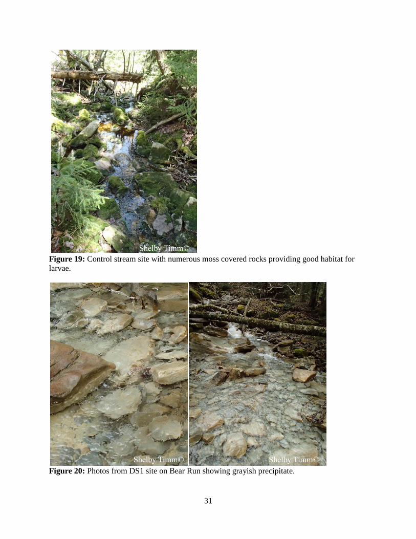
Although liming significantly increased the pH as intended, I observed other differences

in stream characteristics below the DAL site, such as increased sedimentation (Figure 18),

compared to control streams (Figure 19) and the presence of a grayish precipitate on the stream

substrate (Figure 20). The grayish substance observed was likely a precipitate of dissolved

aluminum, which occurs when pH levels increase and has been found below lime application in

other streams (LeFevre & Sharpe 2002). Aluminum precipitate decreases macroinvertebrate

abundance, with the greatest impact directly below lime in the mixing zone (Okland & Okland

1986; Gensemer & Playle 1999; LeFevre & Sharpe 2002; Simmons et al 2006), which would

further explain why macroinvertebrate abundance appeared lower downstream of the DAL;

however, this was not quantified.

Figure 18: Direct application lime site in Dogway Fork.

31

Figure 19: Control stream site with numerous moss covered rocks providing good habitat for

larvae.

Figure 20: Photos from DS1 site on Bear Run showing grayish precipitate.

32

My results may indicate that strong selection, where slower growing individuals are

removed from the population, results in lower abundances and reduced intraspecific competition,

which possibly explains both faster growth and higher body condition downstream of DAL.

Plasticity is a trait that allows many species, such as G. porphyriticus, to occupy a range of

environmental conditions. The adaptive nature of the plastic trait is evidenced by the reaction

norm, which is often predictable across populations and characteristic of specific populations

(Stearns 1989; DeWitt et al. 1998). My research demonstrates that G. porphyriticus exhibits

population-level responses to DAL mitigation, which may cause life history shifts in larvae.

Further research is needed to identify specific mechanisms to understand if my observations are

the direct effects of liming, such as increased sedimentation and changes in water chemistry, or

caused by indirect effects, such as alterations in trophic structure, and how these changes

contribute to emergent effects. It is important to further investigate the tradeoffs that are

occurring within individuals with increased growth rates and smaller gape sizes, as well as

differences in diet using gut content analysis to determine if trophic structure has been altered.

33

CHAPTER 2

GYRINOPHILUS PORPHYRITICUS LIFE HISTORY NOTE

Gyrinophilus porphyriticus is a stream associated species and its distribution ranges from

Southern Quebec to Alabama, throughout the Appalachian Mountains (Petranka 1998). Their

distribution covers a large range of latitudes, with southern populations experiencing different

climates than northern populations, contributing to different life history strategies. Previous

research on G. porphyriticus populations in the southern Blue Ridge Mountains reported that

there was no correlation between SVL and age, and suggested that skeletochronology may be an

unreliable technique for aging these populations, which may remain active throughout the year,

due to indistinguishable lines of arrested growth (n=17; Bruce & Castanet 2006).

I collected G. porphyriticus larvae between April 25, 2014 to August 23, 2014 from

multiple populations in the Gauley River watershed in Pocahontas and Greenbrier counties, WV,

in the southern portion of the Monongahela National Forest. I used skeletochronological

analysis of femurs for larval age determination. Age can be determined in amphibians by

counting the number of lines of arrested growth (LAGs) in the cross-sections of the diaphysis of

long bones or phalanges (Castanet et al. 1993). Lines of arrested growth are deposited annually

in temperate regions during winter when growth slows and individuals are less active. My

research shows that there is a significant positive correlation between SVL (mm) and age (years)

in G. porphyriticus (Figure 1; p < 0.0001, R = 0.669). However, there is a substantial amount of

overlap in SVL between age classes (Table 1), supporting that size classes should not be used to

estimate age. My research indicated that skeletochronology is a reliable method G. porphyriticus

in West Virginian populations that experienced colder winters and therefore experienced a period

of reduced growth that produced reliable and well defined LAGs.

34

Figure 1: Linear correlation for SVL with age, including 95% confidence intervals.

Table 1: Descriptive statistics for larval G. porphyriticus populations in the Monongahela

National Forest. The range and mean for SVL ± standard deviation was calculated for each age.

The percentage of each age group from the entire sample (n = 158) is reported.

AGE

Indicators 0 1 2 3 4 5 6

Range (SVL, mm) 25.70-27.00 28.10-36.60 31.05-51.95 32.95-67.75 37.90-64.20 45.35-63.90 51.05-61.67

Mean (SVL, mm) 26.40±0.66 31.03±3.58 38.08±6.19 47.92±7.90 51.26±5.52 55.23±4.90 55.38±4.58

% of Sample 1.91% 3.82% 9.55% 41.40% 26.75% 13.38% 3.18%

35

LITERATURE CITED

Abrams, P. and Rowe, L. 1996. The effects of predation on the age and size of maturity of prey.

Evolution 50: 1052-1061.

Arendt, J.D. 1997. Adaptive intrinsic growth rates: An integration across taxa. The Quarterly

Review of Biology 72: 149-177.

Ashkavandi, S., Gharzi, A., & Abbassi, G.M. 2012. Age determination by skeletochronology in

Rana ridibunda (Anuran:Amphibia). Asian Journal of Experimental Biological Sciences

3(1):156-162.

Beachy, C. K. 1994. Community ecology in streams: Effects of two species of predatory

salamanders on a prey species of salamander. Herpetologica 50: 129-136.

Beachy, C.K. 1995. Effects of larval growth history on metamorphosis in a stream-dwelling

salamander (Desmognathus ochrophaeus). Journal of Herpetology 29: 375-382.

Bervin, K. and Gill, D. 1983. Interpreting geographic variation in life-history traits. American

Zoologist 23: 85-97.

Bishop, S. C. 1941. The salamanders of New York. New York State Museum Bulletin. 324:1-

365.

Bonin, J. 1999. COSEWIC status report on the spring salamander Gyrinophilus porphyriticus in

Canada in COSEWIC assessment and status report on the spring salamander

Gyrinophilus porphyriticus in Canada. Committee on the Status of Endangered Wildlife

in Canada. Ottawa. 1-16 pp.

Bruce, R.C. 1980. A model of the larval period of the Spring Salamander, Gyrinophilus

porphyriticus, based on size-frequency distributions. Herpetologica 36:78-86.

Bruce, R. C. 2005. Theory of complex life cycles: Application in Plethodontid salamanders.

Herpetological Monograpghs 19: 180-207.

Bruce, R.C. & Castanet, J. 2006. Application of skeletochronology in aging larvae of the

salamanders Gyrinophilus porphyriticus and Pseudotriton ruber. Journal of Herpetology

40: 85-90.

Carey, M.P. and Wahl, D.H. 2010. Interactions of multiple predators with different foraging

modes in an aquatic food web. Oecologia 162: 443-452.

Castanet, J., Francillon-Vieillot, H., Meunier, F. J., and Ricqles, A. DE. 1993. Bone and

individual aging. Bone 7: 245-283.

36

Chase, J. 1999. To grow or reproduce? The role of life-history plasticity in food web dynamics.

The American Naturalist 154: 571-586.

Clair, T.A. and Hindar, A. 2005. Liming for the mitigation of acid rain effects in freshwaters: A

review of recent results. Environmental Review 13: 91-128.

Clayton, J. and Menendez, R. 1996. Macroinvertebrate responses to mitigative liming of

Dogway Fork, West Virginia. Restoration Ecology 4: 234-246.

Clayton, J., Dannaway, E., Menendez, R., Rauch, H., Renton, J., Sherlock, S., and Zurbuch, P.

1998. Application of limestone to restore fish communities in acidified streams. North

American Journal of Fisheries Management 18: 347-360.

Clobert, J., Oppliger, A., Sorci, G., Ernande, B., Swallow, J., and Garland, T. 2000. Trade-offs in

phenotypic traits: endurance at birth, growth, survival, predation and susceptibility to

parasitism in a lizard, Lacerta vivipara. Functional Ecology 14: 675-684.

Corn, P. and Bury, B. 1989. Logging in Western Oregon: Responses of headwater habitats and

streams amphibians. Forest Ecology and Management 29: 39-57.

Currens, C., Liss, W., and Hoffman, R. 2007. Impacts of a gape limited brook trout, Salvelinus

fontinalis, on larval Northwestern salamander, Ambystoma gracile, growth: A field

enclosure experiment. Journal of Herpetology 41: 321-324.

DeWitt, T., Sih, A. and Wilson, D. 1998. Costs and limits of phenotypic plasticity. Tree 13: 77-

81.

Driscoll, C., Driscoll, K., Mitchell, M., and Raynal, D. 2003. Effects of acidic deposition on

forest and aquatic ecosystems in New York State. Environmental Pollution 123: 327–

336.

Downey, D., French, C., and Odom, M. 1994. Low cost limestone treatment of acid sensitive

trout streams in the Appalachian mountains of Virginia. Water, Air, and Soil Pollution

77: 49-77.

Edwards, E. 2014. Examining the effects of liming on Gyrinophilus porphyriticus with a

comparison of multiple sampling methods. Theses, Dissertations, and Capstones.

Marshall University. Paper 865.

Eggleton, M.A., Morgan, E.L., and Pennington, W.L. 1996. Effects of Liming on an Acid-

Sensitive Southern Appalachian Stream. Restoration Ecology 4: 247-263.

Engqvist, L. 2005. The mistreatment of covariate interaction terms in linear model analyses of

behavioural and evolutionary ecology studies. Animal Behaviour 70:967-971.

37

Finlay, J. and Vanderburg, V. 2007. Introduced trout sever trophic connections in watersheds:

Consequences for a declining amphibian. Ecology 88: 2187-2198.

Forsman, A. 1994. Growth rate and survival in relation to relative head size in Vipera berus.

Journal of Herpetology 28: 231-238.

Forsman, A. 1996. Body size and net energy gain in gape-limited predators: A model. Journal of

Herpetology 30: 307-319.

Freda, J. and Dunson, W. 1985. Field and laboratory studies of ion balance and growth rates of

Ranid tadpoles chronically exposed to low pH. Copeia 1985: 415-423.

Gensemer, R. and Playle, R. 1999. The bioavailability and toxicity of aluminum in aquatic

environments. Critical Reviews in Environmental Science and Technology 29: 315-450.

Ghalambor, C., McKay, J., Carroll, S., and Reznick, D. 2007. Adaptive versus non-adaptive

phenotypic plasticity and the potential for contemporary adaptation in new environments.

Functional Ecoloty 21: 394-407.

Harfoot, M., Newbold, T., Tittensor, D., Emmott, S., Hutton, J., Lyutsarev, V., Smith, M.,

Scharlemann, J., and Purves, D. 2014. Emergent global patterns of ecosystem structure

and function from a mechanistic general ecosystem model. PLOS Biology 12(4):

e1001841.

Hartel, T., Nemes, S., Cogalniceanu, D., Ollerer, K., Schweiger, O., Moga, C., and Demeter, L.

2007. The effect of fish and aquatic habitat complexity on amphibians. Hydrobiologia

583: 173-182.

Hereford, J. 2009. A quantitative survey of local adaptation and fitness trade-offs. The American

Naturalist 173: 579-588.

Ivahnenko, T., Renton, D., & Rauch, H. 1988. Effects of liming on water quality of two streams

in West Virginia. Water, Air and Soil Pollution 41: 311-357.

Jakob, E.M., Marshall, S.D., & Uetz, G.W. 1996. Estimating fitness: A comparison of body

condition indices. Oikos 77:61-67.

Keener, A. and Sharpe, W. 2005. The effects of doubling limestone sand applications in two

acidic Southwestern Pennsylvania streams. Restoration Ecology 13: 108-119.

Lane, E. W. 1947. Report of the Subcommittee on Sediment Terminology. Transactions

American Geophysical Union 28(6): 936-938.

Leclair, R. & Castanet, J. 1987. A skeletochronological assessment of age and growth in the

frog Rana pipiens Schreber (Amphibia, Anura) from Southwestern Quebec. Copeia

1987(2):361-369.

38

LeFevre, S. and Sharpe, W. 2002. Acid stream water remediation using limestone sand on Bear

Run in Southwestern Pennsylvania. Restoration Ecology 10: 223-236.

Lowe, W. 2003. Linking dispersal to local population dynamics: A case study using a headwater

salamander system. Ecology 84(8): 2145-2154.

Lowe, W. 2005. Factors affecting stage-specific distribution in the stream salamander

Gyrinophilus porphyriticus. Herpetologica 61(2): 135-144.

Lowe, W. and Bolger, D. 2002. Local and landscape-scale predictors of salamander abundance

in New Hampshire headwater streams. Conservation Biology 16: 183-193.

Lowe, W., Likens, G., and Cosentino, B. 2006. Self-organisation in streams: the relationship

between movement behavior and body condition in a headwater salamander. Freshwater

Biology 51: 2052-2062.

Lowe, W., McPeek, M., Likens, G., and Cosentinos, B. 2012. Decoupling of genetic and

phenotypic divergence in a headwater landscape. Molecular Ecology 21: 2399-2409.

Lowe, W., Nislow, K., and Bolger, D. 2004. Stage-specific and interactive effects of

sedimentation and trout on a headwater stream salamander. Ecological applications 14:

164-172.

Luquet, E., Lena, J-P., Miaud, C., and Plenet, S. 2015. Phenotypic divergence of the common

toad (Bufo bufo) along an altitudinal gradient: Evidence for local adaptation. Heredity

114: 69-79.

Mant, R., Jones, D., Reynolds, B., Ormerod, S., and Pullin, A. 2013. A systematic review of the

effectiveness of liming to mitigate impacts of river acidification on fish and

macroinvertebrates. Environmental Pollution 179: 285-293.

Maret, T. and Collins, J. 1996. Effect of prey vulnerability on population size structure of a gape-

limited predator. Ecology 77: 320-324.

McClurg, S., Petty, J.T., Mazik, P., and Clayton, J. 2007. Stream ecosystem response to

limestone treatment in acid impacted watersheds of the Allegheny Plateau. Ecological

Applications 17: 1087-1104.

McDonald, J.H. 2014. Handbook of Biological Statistics (3rd ed.). Sparky House Publishing,

Baltimore, Maryland. This web page contains the content of pages 77-85 in the printed

version.

Mckie, B.G., Petrin, Z., and Malmqvist, B. 2006. Mitigation or disturbance? Effects of liming

on macroinvertebrate assemblage structure and leaf-litter decomposition in the humic

streams of Northern Sweden. Journal of Applied Ecology 43: 780-791.

39

Menendez, R., Clayton, J., and Zurbuch, P. 1996. Chemical and fishery responses to mitigative

liming of an acidic stream, Dogway Fork, West Virginia. Restoration Ecology 4: 220-

233.

Menendez, R., Clayton, J., Zurbuch, P., Sherlock, S., Rauch, H., and Renton, J. 2000. Sand-

sized limestone treatment of streams impacted by acid mine drainage. Water, Air, and

Soil Pollution 124: 411-428.

Ohdachi, S. 1994. Growth, metamorphosis, and gape-limited cannibalism and predation on

tadpoles in larvae of salamanders Hynobius retardatus. Zoological Science 11: 127-131.

Okland, J. and Okland, K. 1986. The effects of acid deposition on benthic animals in lakes and

streams. Experientia 42: 471-486.

Pease, C. and Bull, J. 1988. A critique of methods for measuring life history trade-offs. Journal

of Evolutionary Biology 1: 293-303.

Petranka, J.W. 1998. Salamanders of the United States and Canada. Smithsonian Institution

Press, Washington, D.C.

Pierce, B. 1985. Acid tolerance in amphibians. Bioscience 35: 239-243.

Pope, K. and Matthews, K. 2002. Influence of anuran prey on the condition and distribution of

Rana mucosa in the Sierra Nevade. Herpetologica 58: 354-363.

Resetarits, W. 1991. Ecological interactions among predators in experimental stream

communities. Ecology 72: 1782-1793.

Resetarits, W. 1995. Competitive asymmetry and coexistence in size-structured populations of

Brook Trout and Spring Salamanders. Oikos 73: 188-198.

Reynolds, C.S. and Elliott, J.A. 2012. Complexity and emergence in aquatic ecosystems:

predictability in aquatic ecosystem responses. Freshwater Biology 57: 74-90.

Roff, D. 2000. Trade-offs between growth and reproduction: An analysis of the quantitative

genetic evidence. Journal of Evolutionary Biology 13: 434-445.

Rohr, J., Elskus, A., Shepherd, B., Crowley, P., McCarthy, T., Niedzwiecki, J., Sager, T., Sih,

A., and Palmer, B. 2004. Ecological Applications 14: 1028-1040.

Rowe, L. and Ludwig, D. 1991. Size and timing of metamorphosis in complex life cycles: Time

constraints and variation. Ecology 72: 413-427.

SAS Institute Inc. 2013. SAS® 9.4 Guide to Software Updates. Cary, NC: SAS Institute Inc.

40

Schulte-Hostedde, A., Zinner, B., Millar, J., and Hickling, G. 2005. Restitution of mass-size

residuals: Validating body condition indices. Ecology 86: 155-163.

Sih, A., Petranka, J., and Kats, L. 1988. The dynamics of prey refuge use: A model and tests with

sunfish and salamander larvae. American Naturalist 132: 463-483.

Sih, A. and Kats, L. 1991. Effects of refuge availability on the responses of salamander larvae to

chemical cues from predatory green sunfish. Animal Behavior 42: 330-332.

Simmons, J., Andrew, T., Arnold, A., Bee, N., Bennett, J., Grundman, M., Johnson, K., and

Shepherd, R. 2006. Small-scale chemical changes by in-stream limestone sand additions

to streams. Mine Water and the Environment 25: 241-245.

Skei, J. and Dolmen, D. 2006. Effects of pH, aluminum, and soft water on larvae of the

amphibians Bufo bufo and Triturus vulgaris. Canadian Journal of Zoology 84: 1668-

1677.

Smirina, E.M. 1994. Age determination and longevity in amphibians. Gerontology 40:133-146.

Smith-Gill, S. 1983. Developmental plasticity: Developmental conversion versus phenotypic

modulation. American Zoologist 23: 47-55.

Socha, M. & Ogielska, M. 2010. Age structure, size and growth rate of water frogs from central

European natural Pelophylax ridibundus-Pelophylas esculentus mixed populations

estimated by skeletochronology. Amphibia-Reptilia 31:239-250.

Sokal, R. R., and F. J. Rolhf. 1981. Biometry. 2nd edition. W. H. Freeman. San Francisco, CA.

Stearns, S. C. 1989. The evolutionary significance of phenotypic plasticity. Bioscience 39: 436-

445.

Stearns, S. C. 1992. The Evolution of Life Histories. Oxford University Press, Oxford, U.K.

Sverdrup, H. 1986. The dissolution efficiency for different stream liming methods. Water, Air

and Soil Pollution 31: 827-837.

Teplitsky, C., Rasanent, K., Laurila, A. 2007. Adaptive plasticity in stressful environments:

Acidity constrains inducible defenses in Rana arvalis. Evolutionary Ecology Research 9:

447-458.

Urban, M. 2008. Salamander evolution across a latitudinal cline in gape-limited predation risk.

Oikos 117: 1037-1049.

Wake, D.B. & Castanet, J. 1995. A skeletochronological study of growth and age in relation to

adult size in Batrachoseps attenuates. Journal of Herpetology 29(1):60-65.

41

Walls, S., Belanger, S., and Blaustein, A. 1993. Morphological variation in a larval salamander:

Dietary induction of plasticity in head shape. Oecologia 96: 162-168.

Waters, T.F. 1995. Sediment in streams- Sources, biological effects and control. American

Fisheries Society Monograph 7. American Fisheries Society, Bethesda, MD.

Welsh, H. and Droege, S. 2001. A case for using Plethodontid Salamanders for monitoring

biodiversity and ecosystem integrity of North American forests. Conservation Biology.

15: 558-569.

Welsh, H.H. and Ollivier, L.M. 1998. Stream amphibians as indicators of ecosystem stress: a

case study from California’s redwoods. Ecological Applications 8: 1118-1132.

Werner, E. and Anholt, B. 1993. Ecological consequences of the trade-off between growth and

mortality rates mediated by foraging activity. The American Naturalist 142: 242-272.

Wilbur, H. and Collins, J. 1973. Ecological aspects of amphibian metamorphosis. Science 182:

1305-1314.

Wilbur, H. 1980. Complex life cycles. Annual Review of Ecological Systems 11: 67-93.

Zaret, T. 1980. Predation and freshwater communities. Yale University Press, New Haven,

Connecticut, USA.

42

APPENDIX A

Figure 1: Cross section. No LAGs are present, but the hatching line (HL) is clearly seen. This

larva is a young of the year (0 years).

Figure 2: Cross section. One LAG is present, with the HL clearly seen. This individual was

collected at the end of the sampling season; therefore, there is growth behind the LAG, and the

peripheral edge is not considered a LAG. This larva is one year.

HL

HL 1

43

Figure 3: Cross section. Two LAGs are present, with the HL clearly seen. This individual was

collected at the end of the sampling season; therefore, there is growth behind the LAG, and the

peripheral edge is not considered a LAG. This larva is two years.

HL

1

2

44

Figure 4: Cross section. Three LAGs are present, with the HL clearly seen. This individual

was collected at the beginning of the sampling season; therefore, there is no growth behind the

most recent LAG so the peripheral edge of the bone is considered a LAG. This larva is three

years.

1 2 3

HL

45

Figure 5: Cross section. Four LAGs are present, with the HL clearly seen. This individual was

collected at the beginning of the sampling season; therefore, there is no growth behind the most

recent LAG so the peripheral edge of the bone is considered a LAG. This larva is four years.

HL

4 3 2

1

46

Figure 6: Cross section. Five LAGs are present, with the HL clearly seen. This individual was

collected at the beginning of the sampling season; therefore, there is no growth behind the most

recent LAG so the peripheral edge of the bone is considered a LAG. This larva is five years.

HL

1 2

3

4

5

47

Figure 7: Cross section. Six LAGs are present, with the HL clearly seen. This individual was

collected at the beginning of the sampling season; therefore, there is no growth behind the most

recent LAG so the peripheral edge of the bone is considered a LAG. This larva is six years.

1 2 3 4 5

6

HL

48