Embed Size (px)
Citation preview
Pooling Risk Among Countries1
Jean Imbs Paolo Mauro HEC Lausanne International Monetary Fund
Swiss Finance Institute CEPR
August 2007
Abstract We identify the groups of countries where international risk-sharing opportunities are most attractive. We show that the bulk of risk-sharing gains can be achieved in groups consisting ofas few as seven members, and that further marginal benefits quickly become negligible. Formany such small groups, the welfare gains associated with risk sharing are far larger than Lucas’s classic calibration suggested for the United States, under similar assumptions onutility. Why do we not observe more arrangements of this type? Our results suggest that large welfare gains can only be achieved within groups where contracts are relatively difficult to enforce. International diversification can thus yield substantial gains, but they may remain untapped owing to potential partners’ weak institutional quality and a history of default oninternational obligations. Noting that existing risk-sharing arrangements often have a regional dimension, we speculate that shared economic interests such as common trade may helpsustain such arrangements, though risk-sharing gains are smaller when membership isconstrained on a regional basis. JEL Classification Numbers: E21, E32, E34, F41 Keywords: Risk Sharing, Diversification, Enforceability
1 The first draft of this paper was written while Imbs was a resident scholar in the IMF’s Research Department. The paper was completed while Imbs was visiting the Hong Kong Institute for Monetary Research, whose hospitality is gratefully acknowledged. Financial support was provided by the National Center of Competence in Research “Financial Valuation and Risk Management”. The National Centers of Competence in Research (NCCR) are a research instrument of the Swiss National Science Foundation. We are grateful to Tamim Bayoumi, Mick Devereux, Michael Kremer, Raghuram Rajan, and Jaume Ventura for insightful suggestions; to Nicolas Metzger, José Romero, and especially Michael Callen for superb research assistance; and to Jean Salvati and especially Huigang Chen and Alin Mirastean for invaluable help in programming and computational support. All errors are our own. Corresponding author: Imbs - HEC Lausanne - 1015 Lausanne, Switzerland. [email protected].

1
I. INTRODUCTION
Under perfect international risk sharing, country-specific risk is insured away as citizens hold
and consume out of an identical portfolio of state-dependent assets. Full diversification entails
payments going from booming economies into ones in recession, and requires an ability to
monitor and enforce contractual arrangements.2 If monitoring and enforcement become difficult
or costly as the number of countries involved increases, then the question of who to share risk
with acquires key importance. Choosing a membership then involves a tradeoff between
diversification benefits and monitoring costs, and may result in groups that involve a limited
number of countries. This paper focuses on the benefits side, and empirically estimates risk
diversification opportunities for all possible groups that exist in a sample of 74 countries.
The relevance of the question is highlighted by the existence of a few schemes that indeed have
sought to foster international sharing of macroeconomic risks within “clubs” (or “pools”)
consisting of a limited number of countries, rather than worldwide. These schemes include, for
example, pooling arrangements for international reserves, such as the Chiang Mai initiative, the
Latin American Reserve Fund (FLAR), or networks of bilateral swap arrangements among the
G-10 in the 1960s-70s and among the European countries during the run up to the establishment
of the Euro. In fact a number of schemes have been proposed, which seek to achieve
international sharing of GDP risk among small groups of countries, including Robert C.
Merton’s (1990, 2000) suggestions regarding networks of bilateral swaps of GDP-linked
income streams.3 More generally, currency and trade unions may also lead to greater
international financial integration, and could therefore foster greater mutual risk sharing.
Our main innovation consists in running a systematic search on all possible country groupings,
using the variance-covariance matrix for output growth rates observed in standard international
data for 74 countries at various levels of economic and financial development. We take these 2 On the implications of imperfect contract enforcement for the extent of feasible risk sharing, the business cycle, and the ability to reproduce otherwise puzzling features of the data, see for instance Kehoe and Perri (2002) and Kocherlakota (1996).
3 On FLAR, see Eichengreen (2006) and www.flar.net; on the Chiang Mai initiative, see Park and Wang (2005), and http://aric.adb.org; on the earlier European experience, see Eichengreen and Wyplosz (1993). On sharing of GDP risks more generally see Shiller (1993); and Borensztein and Mauro (2004) for a review of the literature.
2
covariances as given and exogenous, and rely on an algorithm that makes it possible to draw up
an inventory of potential income insurance opportunities and to isolate the specific country
groupings that minimize poolwide output growth volatility or maximize welfare diversification
gains, for any possible pool size.
We find that pooling risk among countries can deliver sizable welfare gains. Substantial gains
can obtain in pools consisting of a handful of countries, and marginal gains decline quickly for
groups beyond six or seven members. We find that many small pools—not surprisingly,
involving relatively volatile economies—yield risk-sharing gains more than ten times what
Lucas found for the United States, even though we use a similar theoretical framework.4 But if
large welfare gains can be attained by pooling with a few other countries, why do these
arrangements not emerge spontaneously more often? Unsurprisingly, the largest gains are
attained among heterogeneous economies, in terms of business cycles characteristics, but also
institutional quality, income level, and geographic location. We show that potential
diversification gains are far smaller when pools are formed within the sub-sample of countries
characterized by high institutional quality and an unblemished repayment record. We conjecture
that enforcement may be more difficult for heterogeneous groupings, or for groupings that
involve countries whose institutional quality and perceived creditworthiness are lower.
Welfare gains are on average considerably lower when pools are constrained to be formed
within a particular region or a given income category. Nevertheless, sizable welfare gains are
sometimes attainable through small pools of countries within a region, for instance when they
include some countries whose perceived international creditworthiness is relatively low. In
addition, the few pooling arrangements observed in practice often involve a regional element,
perhaps reflecting cultural and political ties, trade linkages, or a mutual interest in each other’s
economic performance, including a desire to avoid crises in neighboring countries. We
conjecture that the positive impact of trade linkages on contract enforceability may in some
cases dominate their negative impact on diversification opportunities. Trading partners are well
known to have synchronized cycles—see for example Frankel and Rose, 1998. We also estimate
4 Pallage and Robe (2003) show that the welfare cost of economic fluctuations is far larger in developing countries than in advanced economies. We go one step further, and investigate how quickly these gains accrue as the number of participants increases; moreover, we estimate the gains for vast numbers of possible country groupings.

3
the risk-sharing benefits provided by existing reserve-pooling arrangements or free trade areas,
and compare them with the benefits that could be provided by pools of similar size chosen in an
unconstrained manner from the whole sample. The results are consistent with the view that
contract enforceability is an important consideration.
This study is closely related to three strands of the literature. First we build on the extensive
work evaluating the gains from international risk sharing (see, for example, Cole and Obstfeld,
1991; Tesar, 1993; Lewis, 1996; van Wincoop, 1999 or Athanasoulis and van Wincoop, 2000).
In particular, our welfare analysis is largely based on Lewis (2000) and Obstfeld (1994), though
we focus on the relative magnitude of the risk-sharing opportunities provided by different
groupings, rather than their absolute size. Second, an important ingredient in our framework
relates to the international comovement of macroeconomic variables, the object of a large
empirical literature (including Backus, Kehoe and Kydland, 1994; Kehoe and Perri, 2002; Imbs,
2004; and Baxter and Kouparitsas, 2005). Third, any study on the relative desirability of
different country groupings is related to the vast literature on optimum currency areas, going
back to Mundell’s (1961) seminal work, and more recently including Bayoumi and Eichengreen
(1994), Alesina and Barro (2002), and Alesina, Barro, and Tenreyro (2003). At the same time,
optimal pools of countries from a risk-sharing point of view are certain not to coincide with
optimal currency areas.5
The paper is organized as follows. Section II presents a refresher on international risk sharing in
theory, and outlines how we handle the combinatorial problem. Section III presents our general
results on the potential for risk-sharing gains in the sample of countries for which we have data.
In Section IV, we estimate the extent to which the potential for risk sharing is reduced when
countries can only choose their partners within a constrained universe: we focus, for example,
on regional constraints, and on the need for countries to have sufficiently strong institutional
quality in order to be trusted. Section V concludes.
5 Historically, schemes to pool international reserves have often emerged—most notably in the case of the European countries—in a broader context of efforts to establish the conditions for common currencies. However, highly correlated shocks, which militate in favor of a common currency area, reduce diversification opportunities and thus the appeal of pooling arrangements.
4
II. METHODOLOGY
We first go through a quick refresher of the theory underpinning the welfare gains resulting
from risk sharing. We then discuss the algorithms involved in our search for optimal pools of
countries.
A. Risk-Sharing, Volatility, and Welfare
We are interested in the behavior of income and consumption for the countries that are members
of a “pool,” which we define as a group of countries that engage in complete risk sharing with
each other.6 A standard assumption is that under complete markets each country issues and
trades claims on its uncertain future output. These claims pay a share of a country’s future
output, regardless of the state of nature; their payment streams can be interpreted as mimicking
a mutual fund that owns the totality of a country’s productive unit. The same results hold with a
full set of Arrow-Debreu securities (which provide a payment in a given state of nature) or as
the result of optimization by a benevolent social planner.
As is well known, under complete markets each country consumes a fixed share of aggregate
output, given by the country’s share in the aggregate long-run present discounted value of future
poolwide output (see, for example, Obstfeld and Rogoff, 1996). For our purposes, the key
implication from this setup is that, in each period, the growth rate of consumption for any
country in the pool will be the same as the growth rate of aggregate income for the pool, and
will thus fluctuate along with uninsurable poolwide risk. This underpins our focus on the
standard deviation of the growth rate of poolwide GDP, and its comparison with the volatility of
individual country output. Our conclusions are similar when we use the volatility of individual
country consumption instead of output. These results are not reported for the sake of brevity.
Concretely, two types of arrangements could implement the type of risk sharing consistent with
this setup. Under the first, countries in the pool would issue claims on their output as proposed
by Shiller (1993). Capital controls vis-à-vis nonmembers would then ensure that only the
6 Throughout this paper, we assume that countries in a pool would share their entire output streams. In an extension available upon request, we also ask which country groupings yield the greatest risk diversification benefits for a given absolute size of the risk-sharing contract, for example, a US$1 contract, or a US$1 billion contract. The broad findings are similar to those presented here.
5
residents of countries in the pool have access to such securities. The second type of arrangement
would consist of GDP swaps, along the lines proposed by Merton (1990, 2000), either as a
network of bilateral swaps, or as swaps intermediated by a central entity for the pool. Under the
swaps, each period, each country would pay the others the net difference between its current
output and its share in poolwide output, as warranted by its long-run share of poolwide output or
wealth. Differences in expected growth rates across participant countries will be reflected in
their contractual shares of poolwide aggregate output. There would be no need for capital
controls: participation in the network of swaps would define the pool, which might require that
all participants agree to further bilateral swaps with non-members.
Under either arrangement, booming economies might have an incentive to default on their
commitment to pay part of their income to foreign holders of their securities. The paper seeks to
quantify the benefits of risk diversification, and does not focus on the costs of default. But if
preventing default entails costly monitoring and/or enforcement, and if these costs increase in
the number of participants to an insurance scheme, then a second best may obtain where sharing
risk is done optimally among a few countries. Here, we investigate how the benefits of
international risk sharing change with the number of countries involved. This is reminiscent of
Solnik (1974) who asked a similar question on diversification gains, but using asset returns.
To compute welfare we rely on a well-known framework largely based on Lewis (2000) and
similar to Obstfeld (1994). We abstract from non tradability and non separability in utility, and
from the possible impact of uncertainty on growth. These refinements tend to boost the welfare
implications of a given amount of risk sharing, and we conjecture that the same would occur in
our setup. In a related vein, Barro (2007) relies on the possibility of large, disastrous events to
derive much larger welfare costs of business cycles fluctuations than originally measured by
Lucas. We find substantial welfare effects, despite the relative simplicity of the framework
adopted here. We draw on the Epstein and Zin (1989) utility function, and assume that Ct is log-
normally distributed:
( ) ( ) ( ){ } ( )1 11 11 11t t t tU C E U
θθ γθ γβ−− −
− −+
⎡ ⎤= + ⎣ ⎦ and 21
12t t tc c μ σ ε−= + − + with ( )2~ 0,t Nε σ
where c=ln(C); 0<β<1 denotes the subjective discount rate, γ ≥ 0 is the coefficient of relative
risk aversion, and θ is the inverse of the elasticity of intertemporal substitution in consumption.
6
As shown in Lewis (2000), welfare for the representative individual in country j at time t=0 is
given by:
( )( )( )1 1
20 0
11 exp 12
j jj jU C
θ
β θ μ γσ− −
⎧ ⎫⎡ ⎤⎛ ⎞= − − −⎨ ⎬⎜ ⎟⎢ ⎥⎝ ⎠⎣ ⎦⎩ ⎭
The welfare gain for moving from autarky to pooling is expressed as the permanent percent
increase in annual consumption in country j under autarky, δ j, that would make the
representative individual just as well off as under pooling:
( )0 01 , , , ,j j
j jU C U Cδ μ σ μ σ⎡ ⎤ ⎡ ⎤+ = ⎣ ⎦⎣ ⎦ , that is,
( )( )( )
( )( )( )
1 12
01 1
0 2
11 exp 12
111 exp 12
jj
j j
CC
θ
θ
β θ μ γσδ
β θ μ γσ
− −
− −
⎧ ⎫⎡ ⎤⎛ ⎞− − −⎨ ⎬⎜ ⎟⎢ ⎥⎝ ⎠⎣ ⎦⎩ ⎭= −⎧ ⎫⎡ ⎤⎛ ⎞− − −⎨ ⎬⎜ ⎟⎢ ⎥⎝ ⎠⎣ ⎦⎩ ⎭
The welfare gains from risk sharing depend on three factors. First, the difference between
individual and poolwide volatilities, jσ and σ , respectively. Second, the difference between
growth rates within and without the pool, μ and jμ , respectively. Third, the ratio between
initial consumption in autarky, 0jC , and consumption in the pool, 0C , which reflects a (positive
or negative) “entry transfer” in terms of initial consumption that country j pays to (or receives
from) other members for being allowed into the pool. The term “entry transfers” is used as
shorthand. These transfers could take place later in the life of the contract. More important, the
optimal (renegotiation-proof) contract would likely allow the share of poolwide output accruing
to country j to change during the life of the contract, in response to updated information
regarding country j’s long-term expected growth, volatility, and correlation with poolwide
output.
This paper abstracts from intertemporal consumption smoothing. Welfare gains can also result
from self-insurance, via saving and borrowing decisions, rather than internationally. We do not
mean to suggest either approach dominates. Rather the paper follows the international risk-
sharing literature and investigates how quickly welfare gains accrue when insurance is sought
exclusively via international contracts.

7
Solving for entry transfers, Lewis (2000) shows that
( ) 2
0
2 20
11 exp 12
1 1exp 1 exp2 2
j
C HC H
β θ μ γσ
μ γσ β θ μ γσ
⎡ ⎤⎛ ⎞− − −⎜ ⎟⎢ ⎥⎝ ⎠⎣ ⎦=⎛ ⎞ ⎡ ⎤⎛ ⎞− − − −⎜ ⎟ ⎜ ⎟⎢ ⎥⎝ ⎠ ⎝ ⎠⎣ ⎦
where 21
2exp cov( , )j jH μ γσ γ ε ε⎡ ⎤= + −⎣ ⎦ reflects the desirability of country j from the
standpoint of the pool’s hedging motive. Countries characterized by low (or negative)
covariance with the pool will be more likely to receive a net transfer at the beginning of the
arrangement ( 0 0jC C> ). Conversely, countries whose output covaries strongly with poolwide
output will be more likely to make a net payment in order to join the pool (that is, 0 0jC C< ).
In what follows, we compare how countries fare individually and under pooling, using four
approaches. First, we report the standard deviation of the growth rate for individual country
income and poolwide income. This simple approach, focused on pure diversification gains,
conveys most of the key economic intuition. Second, as regards welfare, we consider the case
where expected growth is assumed to be the same for all countries (μ = jμ ) and we abstract
from entry transfers ( 0jC = 0C ). These simplifying assumptions make it possible to focus
narrowly on the welfare implications of the fall in volatility associated with pooling, and follow
directly from Obstfeld (1994). There, the emphasis is on the implications of reducing or
eliminating volatility, rather than on trade in financial assets. Under this approach, welfare is a
monotonic, non-linear transformation of volatility. All results on the relative desirability of
various pools based purely on volatility reduction carry through exactly under this simple
extension to welfare.
Third, we report welfare allowing for entry transfers. More specifically, we compute total
welfare gains as the income-weighted sum of δj across the membership, expressed as a share of
the initial income of the relevant (sub-)universe of countries. Fourth and finally, in Section V
we relax the assumption that growth rates are the same for all countries, and project μ and jμ
using past observed growth rates. The paper thus follows a variety of alternative approaches,
and does so for two reasons. First, we aim to provide a transparent presentation of where the

8
gains are coming from. Second, and perhaps more important, views may differ regarding the
realism of the various components of a risk-sharing contract, e.g. the market determination of
entry transfers, or the provision of insurance against differences in long-run growth as opposed
to temporary fluctuations.
As is well known, the link between welfare and volatility depends on some key properties of the
process generating uncertainty: in particular, insurance against permanent shocks has more
value than against temporary ones (see, for instance, Obstfeld, 1994). We assume throughout
that shocks to consumption follow a random walk. This is not crucial to our purpose, and the
assumption is only maintained so that we can decompose poolwide variances into meaningful
elements (Section III.B). Under trend stationarity, the variance of the poolwide residual is not
the variance of a sum of each member country’s residual, and the difference between the two
has no reason to be negligible.
Under the alternative assumption of trend stationarity, measured uncertainty is higher. Indeed, if
GDP truly has a unit root, the detrended residual will have explosive variance. If on the other
hand GDP is truly trend stationary, the variance of GDP growth will be lower than the true
residual variance. In both cases, measured growth rate volatility is higher when assuming trend
stationarity. But under trend stationarity, the welfare costs of fluctuations are smaller for a given
level of uncertainty. As is well known from Lucas’ (1987) seminal paper, the welfare costs of
fluctuations are then approximately given by 21
2γσ , where γ is the coefficient of risk aversion
and σ2 denotes the variance of residual uncertainty. The two effects on the end measure of
welfare tend to offset one another: in fact, we ran our search algorithm under the assumption of
trend stationarity, and found similar results, not reported for the sake of brevity. We reproduced
almost identically the general shape of minimum variance envelopes for the various country
groupings, and the relative impact of different types of constraints on the universe of countries
that one can pool with. The key simplification for our purposes is therefore that the same type of
process (either stationary or random walk) applies to all countries—an assumption that may
prove difficult to invalidate, given the weakness of standard unit root tests.7
7 Dezhbakhsh and Levy (2003) use frequency analysis to investigate the cross-section of spectra followed by GDP growth rates. They find substantial heterogeneity, but are unable to point to a key determining factor. Aguiar and
(continued)

9
B. Combinatorial Analysis
Searching for pools of countries that yield the lowest possible variance of the growth rate of
aggregate (poolwide) GDP is not straightforward, in light of the vast number of possible
combinations of countries. We consider the N countries in our sample individually, then all of
their possible combinations 2 countries at a time (which equals 2NC ), then 3 at a time (which
equals 3NC ), and so on, where
( )!
! !Np
NCp N p
=−
. As is well known, the total number of
partitions is 1
2 1N
N Np
pC
=
= −∑ , which quickly reaches astronomical levels as N rises. 8
Using a computational algorithm whose details are provided in a Technical Appendix available
upon request, we are able to analyze all possible combinations for any pool size within a
universe of 31 countries, i.e. 2.1 billion combinations. This algorithm can easily handle, for
example, the universe of 26 emerging market countries—about 67 million combinations.
However, when the universe consists of all 74 countries in our sample, the same algorithm only
allows us to analyze all combinations of pools of size 7 or less ( 747C = 1.8 billion). By symmetry,
we can also draw the inventory of all combinations of size 67 or above, since N Np N pC C −= .
Beyond these, we need to resort to an approximation algorithm. When N = 74, the total number
of groups increases to 274=1.9x10²², too large for existing computing power. For each group,
one needs to sum the GDP levels for all countries in the pool, to compute an aggregate growth
rate and the corresponding standard deviation. Even if each operation took a nanosecond to
complete, running an exhaustive search over all possible pools amongst 74 countries would take
hundreds of centuries.
Gopinath (2007) suggest that the random walk assumption may be more appropriate for emerging markets than for advanced countries.
8 The integers in the N-th row in Pascal’s (or Tartaglia’s) triangle represent the number of possible combinations of N objects taken 0 at a time, 1 at a time, 2 at a time, ...and N at a time; the sum of the integers in the N-th row is 2N-1.

10
Approximation method for large samples
For sample sizes where exhaustive inventories are out of reach, we implement recursive
searches. Combinatorial problems similar to those we are tackling are the object of a large
literature in computer sciences revolving around the so-called “Traveling Salesman” problem,
for which well-established approximated solution methods exist. To our knowledge however
none can be applied to our baseline setup. For instance, Han, Ye and Zhang (2002) propose an
approximation algorithm that can be applied to minimize the variance of a sum; but we
minimize the variance of a weighted sum, where the weights themselves depend on the group’s
membership. In Imbs and Mauro (2007), we use the Han, Ye and Zhang (2002) algorithm to
identify risk diversification benefits for a given absolute size of the risk-sharing contract (for
example, a US$1 contract). That exercise involves an unweighted average of GDP growth rates.
Our conclusions are virtually identical.
We first obtain all possible combinations up to the maximum pool size where this is feasible
through an exhaustive search—in our case, all pools of size 7 drawn from the universe of 74
countries. We save not only the best pool of size 7, but also the best W pools of size 7 that
include each of the N countries in the universe under consideration. In our baseline results, we
use W=1351 (74 times 1351 is just below 100,000).
For each of these W N⋅ “seed” pools, we analyze all groups that include the existing members,
plus one of the ( N p− ) remaining countries. Among these, we find the best pool of size 8 (as
well as the W N⋅ best new “seed” pools of size 8). We iterate the procedure. Although there is a
recursive aspect to this, the fact that at each stage we consider the best W pools for each of the N
countries gives plenty of opportunities for countries that are in the best pool of a given size to
drop out at the next increment.
We have verified the reliability of this approximation in four different ways. First, for a number
of the cases where it is possible to run exhaustive searches, we compared the groupings implied
by an exhaustive inventory to the results of our approximation: they were always identical.
Second, we have experimented with different values for W, as low as 2, and have found
systematically the same results as with W=1351. Third, for each pool size p, we have checked
large numbers of random samples of countries. We have not found a single instance in which a

11
pool drawn randomly was preferable to those identified as the best through the approximation
procedure. Fourth, we have run exhaustive searches for all possible combinations of 67 (or
more) countries selected amongst 74. Again, we have found the same optimal pools as those
obtained by running the approximation procedure throughout.
III. RESULTS
In this section we describe our dataset and present our results. We first build intuition through a
simple, single country example. We then present the results pertaining to a “global envelope” of
the groupings that achieve maximal risk-sharing gains for all group sizes.
A. Data
Data on yearly real gross domestic product and consumption, evaluated in purchasing power
parity (PPP) U.S. dollars, for the period 1974–2004 are drawn from the World Bank’s World
Development Indicators. Compared with the widely used Penn World Tables (PWT), the World
Bank data base has similar quality, and in fact builds on usually identical information. But it
provides PPP-adjusted data until 2004 rather than 2000. We cross-checked the two data bases
over the period covered by both, and are confident the results are largely unaffected if we use
PWT.
This yields a sample of 25 advanced countries, 26 emerging market countries, and 23
developing countries with complete coverage and data of reasonable quality. (The full country
list is provided in Appendix Table 1). Advanced countries are defined as in the International
Monetary Fund’s World Economic Outlook. The remaining countries are considered emerging if
they are included in either the stock-market-based International Financial Corporation’s Major
Index (2005), or JPMorgan’s EMBI Global Index (2005), which includes countries that issue
bonds on international markets. The rest are classified as developing.
Throughout the paper, in line with the bulk of the literature on international risk sharing, we
assume that PPP holds. This corresponds to the notion that risk sharing is contracted on a pre-
agreed exchange rate, possibly one that is expected to prevail in the long run. While standard,
this is an important assumption. Previous studies (for example, Backus and Smith, 1993; and
Ravn, 2001) have established that real exchange rate fluctuations worsen the case for
international risk sharing. Indeed, GDP data at market exchange rates would imply far higher
12
volatility—harder to hedge through international risk sharing. To compute trade integration, the
data on exports (in U.S. dollars at current prices) are drawn from the IMF’s Direction of Trade
Statistics, and the data on GDP (in U.S. dollars at current prices) are from the IMF’s World
Economic Outlook database.
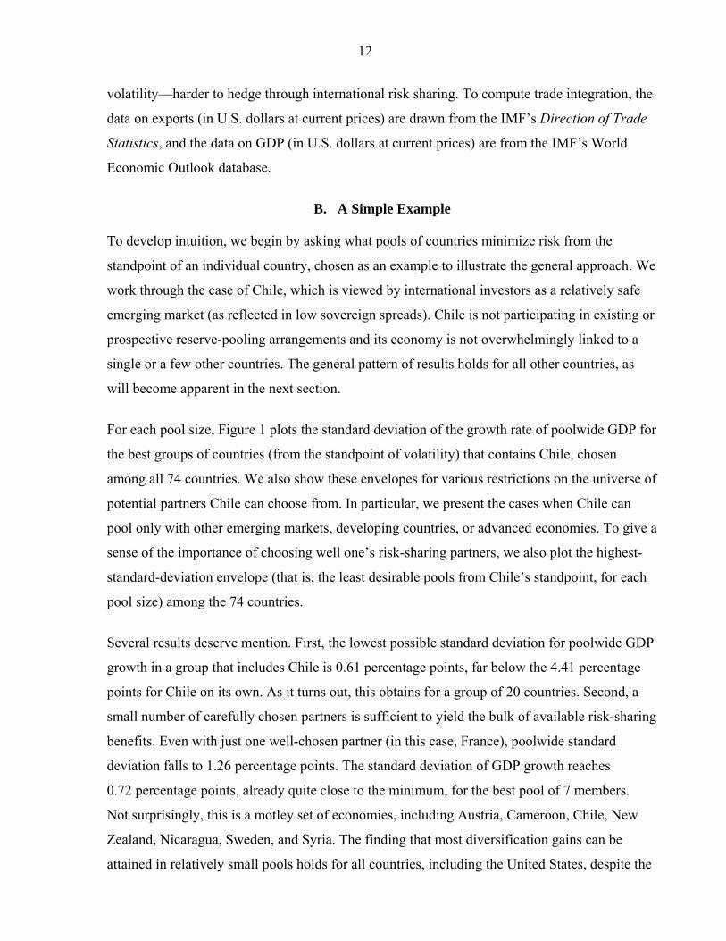
B. A Simple Example
To develop intuition, we begin by asking what pools of countries minimize risk from the
standpoint of an individual country, chosen as an example to illustrate the general approach. We
work through the case of Chile, which is viewed by international investors as a relatively safe
emerging market (as reflected in low sovereign spreads). Chile is not participating in existing or
prospective reserve-pooling arrangements and its economy is not overwhelmingly linked to a
single or a few other countries. The general pattern of results holds for all other countries, as
will become apparent in the next section.
For each pool size, Figure 1 plots the standard deviation of the growth rate of poolwide GDP for
the best groups of countries (from the standpoint of volatility) that contains Chile, chosen
among all 74 countries. We also show these envelopes for various restrictions on the universe of
potential partners Chile can choose from. In particular, we present the cases when Chile can
pool only with other emerging markets, developing countries, or advanced economies. To give a
sense of the importance of choosing well one’s risk-sharing partners, we also plot the highest-
standard-deviation envelope (that is, the least desirable pools from Chile’s standpoint, for each
pool size) among the 74 countries.
Several results deserve mention. First, the lowest possible standard deviation for poolwide GDP
growth in a group that includes Chile is 0.61 percentage points, far below the 4.41 percentage
points for Chile on its own. As it turns out, this obtains for a group of 20 countries. Second, a
small number of carefully chosen partners is sufficient to yield the bulk of available risk-sharing
benefits. Even with just one well-chosen partner (in this case, France), poolwide standard
deviation falls to 1.26 percentage points. The standard deviation of GDP growth reaches
0.72 percentage points, already quite close to the minimum, for the best pool of 7 members.
Not surprisingly, this is a motley set of economies, including Austria, Cameroon, Chile, New
Zealand, Nicaragua, Sweden, and Syria. The finding that most diversification gains can be
attained in relatively small pools holds for all countries, including the United States, despite the

13
large size of the U.S. economy. Pooling with another five or six well-chosen economies
(including Japan, in the first instance) would imply a near halving of the volatility faced by U.S.
residents. This result is reminiscent of the well-known finding in finance that a small set of
stocks is often sufficient to provide most of the diversification opportunities available by
holding the entire stock market (Solnik, 1974).
We later discuss whether all potential partners would want to participate in this agreement from
the strict standpoint of a reduction in volatility. For the time being, however, it is interesting to
note that this is a Pareto improvement compared with the status quo: focusing exclusively on
volatility reduction, each of the countries included is far better off in this pool than on its own.
Indeed, the lowest-standard-deviation envelope shown in Figure 1 looks almost identical if one
adds the constraint that pools should be Pareto improving, i.e. that volatility be lower for all
participants under pooling than in autarky.
Third, marginal gains quickly become small. Based on the volatility criterion they become
negative for groups above 20 members, and more visibly negative as the pool size
increases further than, say, 30 members. Beyond a certain pool size, covariance benefits
are no longer significant, and the pool starts having to include countries that have
relatively high volatility. Note that these results go through exactly under the Obstfeld
(1994) approach, in which welfare is a monotonic transformation of volatility. The same
pools that provide the lowest volatility also yield the highest welfare. Marginal gains will
no longer be negative, however, when allowing for the payment of entry transfers (i.e., for
differences between 0jC and 0C ). Under that setup, countries whose output properties
would tend to increase the overall volatility of the pool could pay existing members in
order to be allowed into the pool, and everybody would be better off.
Finally, the (upper) envelope corresponding to the worst possible pools of each size highlights
the importance of choosing one’s partners carefully: at small pool sizes, one runs the risk of
achieving higher volatility in a poorly chosen pool than in autarky. In the paper, we sometimes
note, but typically do not focus on, the exact identities of the countries that form the best group.
In general, poolwide uncertainty for the lowest volatility group is only marginally below that for
the groups with the second or third lowest volatilities (or even higher). Given that the

14
differences are so small, it is likely that considerations outside our analysis may lead countries
not to choose the absolute best.
We emphasize the extent to which various types of (economically relevant) constraints may
reduce the maximum possible risk diversification benefits. For example, Figure 1 also reports
the extent to which possible gains decline when the universe of countries that Chile can choose
from is constrained by the level of economic and financial development, or geographically. The
lowest possible standard deviation amounts to 0.61 percentage point when Chile is allowed to
choose its pooling partners among all 74 countries, but 0.87 percentage point when it is
constrained to pool with advanced countries only, 1.07 percentage point within the universe of
emerging markets only, and 1.91 percentage points when pooling within Latin America only.
Risk-sharing agreements that are based on common geographic origins, or restricted to countries
within a given range of per capita income, provide smaller gains than do pools formed by
choosing from the unconstrained, worldwide sample.
Variance Decomposition
To illustrate the sources of risk diversification gains, it is useful to decompose the variance of
the growth rate of poolwide income into a weighted average of the variances of individual
countries’ growth rates and a weighted sum of all bilateral covariances. In other words,
2
1 1 1( ) ( ) ( ) ( , )
p p p p
p i i i i i j i ji i i j
Var g Var w g w Var g w w Cov g g= = =
= = +∑ ∑ ∑∑ for ; 1,...i j i p≠ =
where wi denotes the share of country i in the pool’s production, gp is the growth of aggregate
GDP for a pool of p countries, and individual countries’ growth rates are denoted by gi.
Countries are attractive partners to the extent that they have low variances and low (or, even
better, negative) covariances with other members of the pool.
Decomposing poolwide variance for the “best” pool of each pool size, it is possible to show (as
we do in Imbs and Mauro, 2007) that diversification gains for pool sizes up to about seven
countries stem from both the addition of countries with lower volatility than Chile’s and low (or
negative) covariances. The first few countries have both low individual variances and negative
covariances with Chile (as well as, importantly, with each other). However, the covariance gains
diminish rapidly, as the sum of all bilateral covariances starts increasing again. From pool size

15
of about seven onwards, the remaining diversification gains are accounted for almost
exclusively by the addition of countries with lower variance than Chile, but not with negative
average covariances with the rest of the membership.
Would all potential pool members agree to join?
Two potential obstacles seem especially relevant to the ability to form the pools that the method
used above would indicate as optimal for Chile. First, other potential participants may face more
attractive alternatives—an issue that we begin to analyze in this section. Second, there may be
concerns that the risk-sharing contract would not be enforceable—an issue that we address later.
For the time being, we continue to assume away the possibility of entry transfers. As mentioned
above, for each pool size, all countries involved are better off in the pool than on their own.9 But
for each country to agree to participate in the risk-sharing scheme, Pareto improvement is only a
necessary condition: the proposed pool must be the best one possible from the standpoint of
each potential member; indeed, we will define as “stable” those pools with this property.
We focus once again on the Chilean case, where the lowest standard deviation of poolwide
growth is obtained for a group of 20 member countries, listed in Figure 2. On the basis of
volatility reduction, not a single one of the nineteen countries party to Chile’s
optimal grouping would participate in the agreement. They all have more attractive alternatives
available. Figure 2 plots the minimum standard deviation envelope for the countries that form
the pool with minimal variance from Chile’s standpoint. All potential participants would prefer
alternative agreements that would provide them with even lower volatilities, typically by around
0.1 percentage point.
We illustrate the implications of requiring that a pool of a given size be “stable.” Table 1 reports
the standard deviation of poolwide growth for the thus-defined stable pools including Chile. We
focus on sizes up to seven because of computational constraints. Stable pools usually provide
lower diversification benefits than unconstrained groupings. Thus, the requirement that a pool
be stable acts to reduce potential diversification gains, even if only by relatively small amounts.
9 The only exception is the envelope for the Latin American sample, where the Pareto-improving standard deviations are often somewhat above those reported in Figure 1.

16
The results presented in this section are confirmed and generalized in the next. On the basis of
risk diversification alone, there is little need for arrangements including many countries, as long
as partners are chosen carefully. Welfare gains can in principle be sizeable even in small pools
formed on a regional basis or where membership is constrained to countries with relatively low
economic development. However, pools that deliver the greatest diversification benefits tend to
consist of heterogeneous countries with respect to geography, as well as economic and financial
development. In Section IV, we provide a more systematic analysis of the impact of imposing
constraints on the sample of potential partner countries.
C. Global Diversification
We now generalize our results in an exercise that no longer restricts optimal pools to include
any given country: Figure 3 reports the envelope of minimal volatility for all pool sizes p up to
74. As in the previous section, the bulk of possible diversification gains is attained with
relatively small pools. The global best using the pure volatility criterion is a pool of 17
countries, which delivers a standard deviation equal to 0.50 percentage points.10 However, the
standard deviation is already as low as 0.62 percentage points for the best pool of size 7.11 The
property that diversification gains are achieved within groups consisting of a small number of
countries continues to prevail in this general setup.
The value reported for p=1 corresponds to the standard deviation of the individual growth rate
for the least volatile country during the sample period, namely France. Diversification gains for
specific countries cannot be easily read off the figure, because the identities of countries
involved in the various optimal pools of different sizes may change. But we know the identities
of the relevant groupings, and can thus assess the gains that optimal pooling would provide to
member countries. For example, in the case of the optimal group of size 7, the standard
deviations of individual countries’ growth rates range from 1.44 percentage points for Sweden
to 8.97 percentage points for Nicaragua. The diversification gains are thus distributed unequally,
10 Austria, Bangladesh, Benin, Botswana, Cameroon, Chile, Rep. Congo, Costa Rica, Dominican Republic, El Salvador, Gambia, Iceland, Kenya, Lesotho, New Zealand, Nicaragua, Senegal, Sweden, Syrian Arab Republic, and Zimbabwe.
11 Austria, Colombia, Costa Rica, Dominican Republic, New Zealand, Nicaragua, and Sweden.

17
with far larger gains accruing to countries with more volatile individual growth rates. This
asymmetry will have implications for the “entry transfers” we analyze later on.
The list of countries involved in optimal pools confirms that heterogeneity is key. Interestingly,
the list overlaps quite substantially with that obtained for the case of Chile. Several of the same
countries come up as members of the best pools of smaller sizes (where we run a search over all
possible pools, without any approximation) and continue to be present throughout all optimal
pools for p>7. Again, this is unlikely to be an artifact of our approximation method, despite the
recursive structure it imposes onto the search, because the procedure leaves plenty of
opportunities for countries to drop out of the best pool as size increases. Rather, the evidence
suggests that the sample of countries providing the best mutual hedging properties within a
universe of 74 economies is relatively small and robust. For example, the country with lowest
individual volatility, France, does not enter any of the “best” groupings, likely because its
growth cycle is highly correlated with many other economies in the sample. This reinforces the
empirical relevance of low (or negative) covariances.
From a pure volatility standpoint, the groups that trace the envelope charted in Figure 3 are
by definition both Pareto-improving and stable for a given pool size. And the best pool of
17 countries that attains the lowest standard deviation of aggregate poolwide growth is stable
regardless of pool size considerations: none of the countries that form this globally best pool
would have an incentive to deviate to alternative groups of any size on the basis of volatility
reduction, or indeed an “Obstfeld style” welfare metric that ignores entry transfers. A related
exercise is conducted in somewhat greater detail in the Appendix.
Figure 3 also reports the minimum standard deviation of the poolwide growth rate for sub-
samples constrained to the advanced countries, emerging markets, and developing countries.
While risk diversification gains are substantial within each sub-sample, they are not as large as
in the full universe of countries. The envelopes for emerging and developing economies are
roughly one percentage point above the global envelope, for all p. For p<3, the global envelope
and that corresponding to advanced economies coincide, but for larger pool sizes even advanced
countries are considerably better off in pools that allow them to share risk with emerging or
developing countries. Advanced economies achieve somewhat smaller gains, which is

18
consistent with their lower volatility and internationally correlated business cycles. The rapid
exhaustion of diversification opportunities continues to hold in all three sub-samples.
Welfare Gains
We now turn to welfare, and allow for the payment of entry transfers. We still constrain the
expected growth rate to be the same for all countries—an assumption we relax in Section V.
Figure 4 reports the highest (total income-weighted) welfare gains 01
Nj j
j
Yδ=∑ for pools of each
size, normalized by total income for the whole (sub-)universe of countries. The total gains are
monotonically increasing with pool size, and attain a maximum when the entire (sub-)universe
of countries under consideration are pooling together. Just as volatility decreased rapidly in the
number of member countries, welfare gains are large for small-sized groupings, and marginal
gains peter out for pools beyond seven or eight members. Again, the rapid decline in marginal
welfare gains holds when the exercise is conducted for sub-samples of countries consisting of
only advanced, emerging, or developing countries.
The pool formed by the entire 74-country sample for which we have data delivers total gains
amounting to 1.9 percent of initial worldwide income (Table 2). Even allowing for entry
transfers, the gains are far larger for those groups of countries that start out with higher volatility
prior to pooling. As a share of initial income for the group under consideration, total (income-
weighted) welfare gains amount to 0.7 percent for advanced countries, 4.4 percent for emerging
markets and up to 7.4 percent for developing countries. The relatively low welfare potential
amongst rich economies may in part reflect that risk sharing gains have already been reaped
there. This is however unlikely to be a major factor. We find similar results (not reported for the
sake of brevity) when consumption data are used instead of production. As is well known,
consumption and output are highly correlated within countries in the data. The main reason why
welfare gains are relatively small in rich countries is likely to be simply that they are less
volatile. Indeed, the size of these gains differs considerably, depending on the country’s
individual volatility under the status quo. In the full sample, the minimum (United States)
annual gains amount to 0.5 percent of initial country income, and the median gain (Dominican
Republic) is 4.1 percent.

19
IV. POOLING RISK WITHIN SUB-SAMPLES
In this section we quantify the foregone diversification and welfare gains implied by the need to
choose one’s pooling partners within specific sub-samples. In particular, we seek to assess the
importance of choosing partner countries where contract enforcement and monitoring may be
easy. We approximate the concept in a variety of ways, splitting our sample according to:
(a) the level of development and country size; (b) institutional quality and past repayment
record on international debt obligations; (c) the degree of international financial integration;
(d) geographical region; and (e) bilateral trade intensity. In all these cases, we present the results
based on simple volatility criteria, as well as welfare computed with and without entry transfers.
We report the main results in Table 3, for the best possible pool of any size. They confirm that
the patterns of rapid declines in volatility and marginal welfare gains hold within each sub-
sample considered in this section. Finally, we consider existing risk-sharing schemes such as the
Chiang-Mai Initiative or FLAR, or other types of existing arrangements whereby participants
have long established cooperation—for example, in the context of a currency union or a trade
agreement. We estimate the extent to which participant countries would be able to obtain larger
welfare gains in pools of the same size if they were to choose their partners in an unconstrained
manner.
In undertaking these exercises, we assume that the variance-covariance matrix of international
output growth rates would not be affected by entering international risk-sharing arrangements.
This is consistent with findings by Doyle and Faust (2005). They show that, despite claims that
rising integration among the G-7 economies has increased cycles synchronization, there is no
evidence of a significant increase in the correlation of output growth rates or other
macroeconomic aggregates. Moreover, a large empirical literature has documented the cross-
sectional properties of international business cycles, which appear to have extremely persistent
determinants, such as trade linkages or patterns of production (see Frankel and Rose, 1998 or
Baxter and Kouparitsas, 2005). These results are consistent with our assumption that the
international covariances in output growth rates are largely time-invariant.

20
A. Level of Development and Country Size
The degree of volatility reduction and welfare gains that can be attained by pooling countries
within categories defined on the basis of the level of economic development is informative in
two respects. First, it helps gauge the potential interest in pooling risk on the part of countries
belonging to different income groups. Second, one might argue that countries are more likely to
engage in risk sharing agreements with members of a similar income group.
In Table 3, we first report for each sub-sample the median value of the standard deviation of
individual countries’ growth rates across the countries within the sub-universe. Then, for each
country we search over all possible pools of any size that it can form together with others
chosen within the sub-sample. We note the lowest achievable standard deviation of poolwide
growth, and report in the second column the median value of that standard deviation across all
countries in the sub-sample. We then compute for each country the welfare gain obtained by
joining its best pool, assuming that all countries have the same expected growth rate and that
there are no entry transfers, following Obstfeld (1994).12 We report in the third column the
median value of these gains across countries in the sub-universe. Finally, we allow entry
transfers and report the sum of the income-weighted welfare gains that would obtain if all
countries in the sub-universe were to join together to form a pool.
For the typical advanced country, the standard deviation of the growth rate can be cut from
2.0 percentage points under autarky to 0.6 percentage points when moving into the lowest-
volatility pool drawn from the entire universe of countries, and 0.9 percentage points when
pooling with other advanced countries only. The corresponding welfare gains can be as high as
1.1 percentage point of annual consumption when pooling within the universe of all countries,
and 0.8 percentage points when pooling among advanced countries only. Allowing for entry
transfers, total welfare gains to the advanced countries (as a share of initial income of all
advanced countries) are 0.8 percent when all countries in the universe for which we have data
are pooling together, and 0.7 percent when all advanced countries are pooling together. The
gains are much larger for emerging markets, and larger still for developing countries: total gains
12 The results correspond to γ = 5, θ = 2, and β =0.95. The paper’s main messages hold for alternative parameter values.

21
as a share of initial income are 4.4 percent when—allowing for entry transfers—all emerging
markets pool together; the same figure amounts to 7.4 percent for developing countries.
Country Size Interest in the risk-sharing gains provided by pooling is likely to be higher for small countries,
which—on average—are prone to greater volatility. The estimates confirm that small countries
(defined as those with a population below 5.2 million in 1970) would attain substantial volatility
reduction through pooling, and the ensuing welfare benefits would be similarly large.
Interestingly, small countries pooling among themselves attain almost as high risk-sharing gains
as they would if they were to pool within the whole universe of countries in our sample, an
indication that small countries as a group are essentially as diverse as the entire sample.
B. Institutional Quality and Past Repayment Record
We explore the effects of restricting the sample on the basis of whether countries have defaulted
in the recent past or whether they receive high scores on measures of institutional quality, and in
particular contract enforcement. We consider two definitions. The first, labeled “excellent
enforceability” includes all countries that were in the top half of the distribution of the
institutional quality index compiled by Kaufmann and others (2005), and that never experienced
severe international repayment difficulties during 1970–2004.13 The second, “above-average
institutional quality” is based on the institutional quality index only. In addition to advanced
countries, the former sample includes four emerging market and developing countries, whereas
the latter includes eight emerging markets and three developing countries.
The median country with excellent enforceability experiences volatility of 2.1 percentage
points. When pooling with other excellent enforceability countries only, volatility can decline to
0.9 percentage points, and further down to 0.6 percentage points when pooling in an
unconstrained universe. Similarly, the median country with above-average institutional quality
has volatility of 2.6 percentage points, which falls to 0.8 percentage point in the best pool within
the same sample, but even further, to 0.6 percentage point, when pooling within the whole
sample. Available income-weighted welfare gains are equivalent to 0.8 percentage points of
13 Default history is drawn from Reinhart, Rogoff and Savastano (2003) and Detragiache and Spilimbergo (2001).

22
annual consumption within the universe of countries with a reputation for “excellent
enforceability”, and 1.0 percentage points within the universe of countries with above-average
institutional quality. In contrast, the gains are much larger in the complementary samples:
5.1 percentage points of annual consumption for “below-excellent enforceability” countries, and
5.4 percentage points for “below-average institutional quality” countries. Potential risk-sharing
gains are smaller within sub-samples consisting of countries with better perceived
enforceability.
On a more optimistic note, however, consider the risk-sharing opportunities available to
those few emerging market and developing countries that are perceived to have excellent
enforceability, but have high volatility (Botswana, Hungary, Malaysia, and South Africa). Their
median volatility declines from 4.1 percentage points of GDP to 2.2 percentage points if they
can pool together, and to 0.9 percentage points if they draw their pooling partners from the
excellent enforceability countries. A similar result holds for emerging market and developing
countries with “above-average institutional quality”. Welfare gains for these countries when
they pool with the rest of the world are 3 percent of initial income. The magnitudes of these
effects illustrate the large welfare potential that could be drawn from improved institutions,
especially as regards contract enforcement. The quality of institutions may therefore have a two-
fold effect on the volatility of consumption. First, as suggested by Acemoglu and others (2003),
they may directly lower output volatility and enable smoother consumption without any need
for international financial arrangements. Second, they may facilitate access to international
contracts and help countries share risk internationally. The results in this section suggest the
latter has large welfare potential.
C. International Financial Integration
To some extent, many countries are already integrated in global financial markets, though the
evidence is overwhelming that markets are still far from complete. A country’s current degree
of international financial integration may provide an indication of its ability to be a credible
participant in pooling arrangements such as those considered in this paper. Moreover, while
existing capital flows may have already delivered some income insurance, we verify in this
section that it is indeed amongst isolated economies (from a financial standpoint) that
international risk sharing has maximal welfare effects.

23
We divide the sample into high integration and low integration countries based on whether they
are in the top or bottom half of the sample when ranked by total foreign assets to GDP, using
the Lane and Milesi-Ferretti (2006) data set. As might be expected, we find that the countries
whose international financial integration is already relatively high have lower interest in further
international risk sharing. The total income-weighted sum of welfare gains (as a share of the
group’s initial income) is 4.2 percent for low-integration countries, and 1.3 percent for high-
integration countries.
Could this difference simply reflect the impact of financial integration on the international
covariance in output growth rates, which we have assumed fixed and exogenous? Evidence in
Kalemli-Ozcan and others (2003) suggests otherwise: financial integration is found to foster
specialization in production, as consumption plans become increasingly decoupled from local
production. If anything, specialization would increase the potential gains from international
diversification.
D. Regional Constraints
In practice, existing or prospective pools are often formed on a regional basis. We analyze the
implications of geographical constraints through a few examples. We estimate the gains that the
advanced European countries would obtain if they were only allowed to pool with other
advanced European countries, and compare them to the gains that would obtain if they were
allowed to pool with all other advanced countries without geographic restrictions. Similarly, we
compare the gains available to Asian emerging or, separately, Latin American emerging market
pools, with the gains obtained within the sample of all emerging markets.
Geographical constraints do not turn out to be very important for advanced European countries,
presumably because they constitute a high proportion of advanced countries, and because the
advanced country cycle has a large worldwide common component. The median advanced
European country can cut its volatility from 1.8 percentage points to 1.0 percentage point in a
pool of advanced European countries, and to a rather similar 0.9 percentage point in a pool of
advanced countries chosen worldwide. The same message holds using welfare gains.
24
In contrast, geographical constraints are more relevant for emerging markets’ ability to diversify
risk. For instance, median volatility for individual Latin American emerging markets equals 4.4
percentage points and can be lowered to 1.9 percentage point by pooling with five well chosen
Latin American emerging markets, but to as low as 1.3 (1.1) percentage point by pooling with
five (ten) emerging markets in the absence of geographical constraints. Similarly, the median
Asian emerging market can reduce its volatility from 3.6 percentage points to 1.8 percentage
points in a pool of seven Asian emerging markets, and to 1.1 percentage points in a pool of ten
emerging markets chosen also from outside the region. The impact of geographical constraints
remains substantial, although it becomes smaller, when measured in terms of welfare. For Latin
American emerging markets, welfare gains can amount to 5.4 percentage points of initial
income when pooling within the whole universe of emerging markets, but also gains of
4.1 percentage points when pooling within emerging Latin America. Asian emerging markets
can obtain welfare gains equivalent to 3.6 percentage points of initial income when pooling
within the whole universe of emerging markets, but also gains of up to 3.0 percentage points
when pooling within emerging Asia. This reflects the strong non-linearity of welfare as a
function of volatility.
In Imbs and Mauro (2007), we show that the costs of regional constraints are even greater when
measured using the number of instances in which countries in a group are simultaneously
affected by pressures on the exchange rate. This is consistent with studies that find a substantial
regional element in currency crises and in international contagion more generally (Glick and
Rose, 1999).
E. Trade Integration
In this sub-section, we explore further the theme of contract enforceability, which we relate
to trade patterns and the associated regional element often observed in actual pooling
arrangements. Trade linkages imply, on the one hand, higher output correlations and thus
reduced diversification possibilities but, on the other hand, greater ability to enforce risk-sharing
contracts, because defaulting partners can be sanctioned via exclusion from goods trade (see, for
example, Rose and Spiegel, 2004). This may explain the regional element observed in actual
pooling arrangements, which suggests that the impact on contract enforceability may in some
cases prevail over the impact on diversification opportunities. While other factors (such as

25
political or cultural links) may also underlie the desire to form regional agreements, direction of
trade data lend themselves naturally to quantitative analysis in the context of our approach.
To measure trade integration within a pool, we sum exports across all pool members as a ratio
to poolwide GDP. We then consider all possible pools and analyze the correlation between this
measure of trade integration with the minimal volatility of poolwide output. As is well known,
trade is substantially lower among emerging markets than it is among advanced countries, and it
is even lower among developing countries. We analyze separately the relationship between
trade integration and poolwide output volatility for all possible pools of (i) advanced economies,
(ii) emerging markets, and (iii) developing countries. The relationship is depicted in Figure 5 for
pool sizes 5 and 10. The results suggest that greater trade integration is clearly associated with
larger minimal poolwide volatility within the universe of emerging markets and, separately,
developing countries. In other words, fewer diversification opportunities are available among
trade partners. The relationship is weaker among advanced economies, where risk-sharing gains
are smaller to begin with.
F. Existing Arrangements
Finally, we consider the potential welfare gains arising from existing risk-sharing arrangements
such as the Chiang-Mai Initiative or FLAR. We also discuss other types of international
agreements, whereby participants have long-established cooperation, for example, in the context
of a currency union or a trade agreement. We then compare such gains to those that the
participant countries would be able to obtain in pools of the same size, drawing their partners
from the whole, unconstrained sample. The objective here is not to assess the desirability of
the membership structure of existing arrangements, but rather to assess the value of well-
established relations of trust, which make it possible to sustain risk-sharing arrangements. Of
course, some welfare gains may already have accrued to participating countries because of the
existing arrangements. In that regard, our estimates refer to the further gains that would be
drawn by moving to full financial integration within an existing group, compared with full
integration in an alternative grouping with an unconstrained membership of the same size. Table 4 notes the median (first row) and minimum (second row) standard deviation of
individual growth rates across participants in the agreements indicated. The third row compares
these with the standard deviation of poolwide growth obtained by pooling with other members

26
of the existing arrangement. The last row reports volatility in the best possible pool of the same
size as the considered arrangement, but chosen within the whole universe of countries.
Substantial gains appear to be available even for the least volatile countries in each
arrangement. For the existing groups considered (with the exception of FLAR), poolwide
volatility is lower than in autarky. Interestingly, keeping size constant, the lowest possible
volatility in a group with unconstrained membership is more than twice smaller than in an
existing agreement. While existing arrangements have the potential to yield substantial welfare
gains, diversification outside of existing membership may yield considerably greater gains. The
last two rows may be interpreted as suggesting that enforcement considerations play a major
role because they appear to outweigh potentially large diversification gains.
V. EXTENSION—POOLING GROWTH RATES
In our baseline approach, we have assumed that expected growth rates are the same for all
countries. In principle, countries with relatively high expected growth rates should be able to
obtain a higher share of poolwide consumption. In practice however, the challenges involved in
predicting growth rates more than a few years ahead make it relatively difficult to incorporate
differences in expected growth in the terms of risk-sharing contracts. As shown by Easterly and
others (1993), country rankings with respect to growth rates change dramatically from one
decade to the next. Similarly, Jones and Olken (2005) document that most countries experience
both growth miracles and failures at some point in their history. It is unlikely that the parties
negotiating the terms of a risk-sharing agreement would be able to come to a common view of
their countries’ relative future growth performance. And the size of the upfront transfers
involved might preclude an agreement. Indeed, this may be a further reason underlying the
limited extent to which risk-sharing arrangements occur in practice among sovereign nations.
Our main interest in this paper relates to the choice of country groupings rather than the optimal
design of the risk-sharing contract. We do not analyze the feasibility and optimality of contracts
allowing countries to change the shares of poolwide income they receive, as expected growth
rates are updated in the light of new information.
Despite these caveats, we now extend the analysis to the case where expected growth rates can
differ across countries. To estimate expected economic growth, we simply consider the naïve
averaging of growth over the entire period under consideration, namely 1975–2004. An
alternative approach would be to follow van Wincoop (1999) and use the predicted growth rate

27
from cross-country or panel growth regressions, which would however lead to more limited
diversity in expected economic growth. In conducting our analysis, we also assume that
individual countries’ growth rates are unaffected by pooling arrangements. Although a possible
concern might be that lower volatility in a pool may come at the expense of lower mean growth,
this seems unlikely in light of the evidence that lower-volatility countries tend to have relatively
high mean growth (Ramey and Ramey, 1995).
Table 5 reports the welfare gains obtained for the case where all 74 countries in our sample pool
together and for the cases where advanced economies, emerging markets, and developing
countries each pool among themselves. The broad pattern of our results holds. In particular,
Figure 6 confirms the existence of high gains at small pool sizes and rapidly declining marginal
gains as pool sizes increase. Compared with the setup where expected growth is assumed to be
the same for all countries (Table 2 and Figure 4), the welfare gains are somewhat larger in most
instances. This is natural, given that there is now scope for trade in an additional market. In fact,
the relatively high heterogeneity in growth histories among emerging markets may also be the
reason why the welfare gains in developing and emerging economies happen to almost overlap
in Figure 6..
VI. CONCLUSION
Although the potential benefits of international risk sharing have long been the subject of
debate, existing studies have focused on the benefits that an individual country would derive
from greater financial integration into the world economy. Full global financial integration has
hitherto proved elusive, presumably owing in part to limited contract enforcement and
monitoring costs. Monitoring and enforcement may be easier within smaller groups of
countries, and we have shown that risk-sharing pools involving a handful of economies can
often provide substantial welfare gains. Then the question of which countries to pool with
becomes of the essence. We present a systematic analysis of which pools of countries would
provide the greatest risk-sharing benefits, under various possible constraints on membership.
Even though our findings rely on a standard theoretical framework, they suggest that the welfare
benefits of international risk sharing can be substantial, and achievable among surprisingly few
countries. If these gains can be achieved within pools consisting of only a handful of countries,
28
why are risk-sharing arrangements, in one guise or another, not more widespread? We
conjecture that contract enforceability imposes major constraints on the country pools that may
emerge in practice. We show that potential welfare gains are relatively small among the
universe of countries with relatively strong institutions and unblemished repayment records. In
a few cases, pools formed on a regional basis, or built upon pre-existing political, economic or
trade relationships can provide substantial diversification gains. This is consistent with the
observation that the few existing pools, or those under discussion, tend to involve a regional
element or pre-existing well-established relations. Samples where enforceability may be easier
also tend to provide smaller diversification opportunities, so that arrangements to pool risk may
not be worthwhile. More generally, international risk sharing may be limited not because the
gains it affords are too small to matter, but rather because contract enforcement may be difficult
exactly where risk-sharing gains would be largest.

29
APPENDIX: “STABLE” POOLS BASED ON VOLATILITY CRITERION
In this appendix, we pursue the analysis of “stable” pools, which—based on a pure volatility
criterion, or a welfare criterion that is a monotonic transformation of volatility—we define as
those in which all proposed members would be willing to participate. In particular, we seek
groups whose total membership would not be better off in alternative pools, on the basis of risk
diversification gains only. This question can be asked either allowing pool sizes to vary, or
holding the pool size fixed. In what follows, we present the results obtained without restricting
the pools’ size. The results for fixed pool sizes are reported in Imbs and Mauro (2007).
We use the following procedure. Without imposing participation by any specific country, we
identify the pool that provides the lowest standard deviation of poolwide growth. We note the
participants in this necessarily stable pool. We then exclude them from the sample and repeat
the exercise, which identifies the participants in a second (somewhat worse off) stable pool. We
iterate the procedure.
From Section III.C, we know the identity of the best stable pool of 17 countries. We take them
out of the sample, look for the best pool among the remaining countries and find that it consists
of the 19 countries listed in the text table below, with volatility of 0.72 percentage point. By
iterating, we find a third stable pool of 14 countries (0.90 percentage point), a fourth of
13 countries (1.46 percentage point), a fifth of 7 countries (1.98 percentage point), and a sixth of
3 countries (3.28 percentage point). One country is left on its own (even though it is not the
most volatile individually). Despite the lack of realism of this exercise, an interesting point that
comes through is that each of the first five stable pools includes a mix of advanced countries,
emerging markets, and developing countries, and from essentially all continents.

30
Stable Pools (Unrestricted Size) Drawing from Full Universe of 74 Countries Pool Size
Standard Deviation (percent)
Members
17 0.50 Austria, Benin, Cameroon, Colombia, Costa Rica, Dominican Republic, El Salvador, Gambia, Ghana, Kenya, New Zealand, Nicaragua, Senegal, Sweden, Syria, Tunisia, Zimbabwe
19 0.72 Algeria, Argentina, Australia, Bangladesh, Bolivia, Republic of Congo, Denmark, France, India, Italy, Korea, Malawi, Mexico, Netherlands, Norway, Pakistan, Peru, Rwanda, Switzerland
14 0.90 Belgium, Canada, China, Egypt, Finland, Gabon, Germany, Hungary, Iceland, Japan, Philippines, Portugal
13 1.46 Botswana, Chile, Ecuador, Greece, Guatemala, Hong Kong SAR, Ireland, Morocco, Paraguay, Singapore, Trinidad and Tobago, United Kingdom, Uruguay
7 1.98 Brazil, Cote d’Ivoire, Indonesia, Luxembourg, Madagascar, Thailand, United States
3
3.28 Malaysia, Togo, Venezuela
Remainder
Lesotho

31
Appendix Table 1. Country Samples
_______________________________________________________________________________________________________
Advanced Economies
[25]
Emerging Markets
[26]
Developing Countries
[23]
Advanced Europe
[18]
Emerging Market Latin America
[11]
Emerging Market Asia [8]
Small Countries [28]
Excellent Enforceability
[29]
Above Average Institutional
Quality [37]
High capital integration countries
[37]
Low capital integration countries
[37]
Australia Argentina Algeria Austria Argentina China Benin Australia Australia Algeria BangladeshAustria Brazil Bangladesh Belgium Brazil India Bolivia Austria Austria Argentina BeninBelgium Chile Benin Denmark Chile Indonesia Botswana Belgium Belgium Australia BoliviaCanada China Bolivia Finland Colombia Korea Congo Rep. Botswana Botswana Austria BrazilHong Kong SAR Colombia Botswana France Dom. Rep. Malaysia Costa Rica Canada Brazil Belgium CameroonDenmark Cote d'Ivoire Cameroon Germany Ecuador Pakistan Denmark Denmark Canada Botswana ColombiaFinland Dom. Rep. Congo Rep. Greece El Salvador Philippines Dom. Rep. Finland Chile Canada Congo Rep.France Ecuador Costa Rica Iceland Mexico Thailand El Salvador France Costa Rica Chile Costa RicaGermany Egypt Gabon Ireland Peru Finland Germany Denmark China Côte d'IvoireGreece El Salvador Gambia Italy Uruguay Gabon Greece Finland Denmark Dominican Rep.Iceland Hungary Ghana Luxembourg Venezuela Gambia Hong Kong France Egypt EcuadorIreland India Guatemala Netherlands HongKong Hungary Germany Finland El SalvadorItaly Indonesia Kenya Norway Iceland Iceland Greece France GabonJapan Korea Lesotho Portugal Ireland Ireland Hong Kong SAR Germany GambiaLuxembourg Malaysia Madagascar Spain Lesotho Italy Hungary Greece GhanaNetherlands Mexico Malawi Sweden Luxembourg Japan Iceland Hong Kong SAR GuatemalaNew Zealand Morocco Nicaragua Switzerland Malawi Luxembourg Ireland Iceland HungaryNorway Pakistan Paraguay United Kingdom NewZealand Malaysia Italy Ireland IndiaPortugal Peru Rwanda Nicaragua Netherlands Japan Italy IndonesiaSingapore Philippines Senegal Norway New Zealand Korea Japan KenyaSpain South Africa Syria Paraguay Norway Luxembourg Korea LesothoSweden Thailand Togo Rwanda Portugal Malaysia Luxembourg MadagascarSwitzerland Tunisia Trin. and Tob. Senegal Singapore Morocco Malaysia MalawiUnited Kingdom Uruguay Singapore SouthAfrica Netherlands Netherlands MexicoUnited States Venezuela Togo Spain New Zealand New Zealand Morocco
Zimbabwe Trin. and Tob. Sweden Norway Norway NicaraguaTunisia Switzerland Portugal Portugal PakistanUruguay United Kingdom Singapore Singapore Paraguay
United States South Africa South Africa PeruSpain Spain PhilippinesSweden Sweden RwandaSwitzerland Switzerland SenegalThailand Syria ThailandTrinidad and TobagoUnited Kingdom TogoUnited Kingdom United States Trin. and Tob.United States Uruguay TunisiaUruguay Venezuela Zimbabwe
Notes: Advanced countries are defined as in the International Monetary Fund’s World Economic Outlook. The remaining countries are emerging if they are included in either the stock-market based International Financial Corporation’s Major Index (2005) or JPMorgan’s EMBI Global Index (2005), which includes countries that issue bonds on international markets. The remaining countries are classified as developing. Small countries are those with a population below 5.2 million in 1975. Above average institutional quality is according to the index of Kaufmann, Kraay, and Mastruzzi (2005). Excellent enforceability is defined as above average institutional quality and no defaults on international debt in 1970-2004 according to Detragiache and Spilimbergo (2001) and Reinhart, Rogoff and Savastano (2003). High (low) capital integration countries are those in the top (bottom) half of the sample when ranked by total foreign assets to GDP. (Foreign assets are from Lane and Milesi-Ferretti, 2006; GDP data in current U.S. dollars are from the IMF’s World Economic Outlook.) GDP data at PPP are from the World Bank’s World Development Indicators.

32
REFERENCES Aguiar, Mark, and Gita Gopinath, 2007, “Emerging Market Business Cycles: The Cycle is
the Trend,” Journal of Political Economy, Vol. 115, No. 1, pp. 69–102. Acemoglu, D., S. Johnson, J. Robinson and Y. Thaicharoen, 2003, Institutional Causes, Macroeconomic Symptoms: Volatility, Crises and Growth, Journal of Mone- tary Economics, v. 50, pp. 49-123 Alesina, Alberto, and Robert J. Barro, “Currency Unions,” Quarterly Journal of Economics,
Vol. 107, No. 2, pp. 409–436. Alesina, Alberto, Robert J. Barro, and Silvana Tenreyro, 2003, “Optimal Currency Areas,”
NBER Macroeconomics Annual 2002, Vol. 17, pp. 301–345 (Cambridge, Massachusetts and London: MIT Press).
Athanasoulis, Stefano G., and Eric van Wincoop, 2000, “Growth Uncertainty and
Risksharing,” Journal of Monetary Economics, Vol. 45, pp. 477–505. Backus, David K., Patrick J. Kehoe, and Finn E. Kydland, 1994, “Dynamics of the Trade
Balance and the Terms of Trade: The J-curve?” American Economic Review, pp. 84–103.
Backus, David K., and Gregor W. Smith, 1993, “Consumption and real exchange rates in
dynamic economies with non-traded goods,” Journal of International Economics, November, Vol. 35, No. 3-4, pp. 297–316.
Barro, Robert, 2007, “On the Welfare Costs of Consumption Uncertainty,” mimeo Harvard
University. Baxter, Marianne, and Michael A. Kouparitsas, 2005, “Determinants of business cycle
comovement: a robust analysis,” Journal of Monetary Economics, January, Vol. 52, No. 1, pp. 113–157.
Bayoumi, Tamim, and Barry Eichengreen, 1994, “One Money or Many? Analyzing the
Prospects for Monetary Unification in Various Parts of the World,” Princeton Studies in International Finance, No. 76.
Borensztein, Eduardo R., and Paolo Mauro, 2004, “The Case for GDP-Indexed Bonds,”
Economic Policy, April, Vol. 19, No. 38, pp. 165–216. Cole, Harold L., and Obstfeld, Maurice, 1991, “Commodity trade and international risk
sharing: How much do financial markets matter?” Journal of Monetary Economics, August, Vol. 28, pp. 3–24.
33
Detragiache, Enrica, and Antonio Spilimbergo, 2001, “Crises and Liquidity–Evidence and Interpretation,” IMF Working Paper 01/02 (Washington: International Monetary Fund).
Dezhbakhsh, Hashem, and Daniel Levy, 2003, “International Evidence on Output
Fluctuations and Shock Persistence”, Journal of Monetary Economics, Vol. 50, pp. 1499-1530.
Doyle, Brian and Jon Faust, 2005, “Breaks in the Variability and Co-Movement of G-7
Economic Growth”, Review of Economics and Statistics, Vol. 87, No. 4, pp. 721-740. Easterly, William, Michael Kremer, Lant Pritchett, and Lawrence H. Summers, 1993, “Good
policy or good luck? Country growth performance and temporary shocks,” Journal of Monetary Economics, Vol. 32, pp. 459–483.
Eichengreen, Barry, 2006, “Insurance Underwriter or Financial Development Fund: What
Role for Reserve Pooling in Latin America?” NBER Working Paper 12451 (Cambridge, Massachusetts: National Bureau of Economic Research).
Eichengreen, Barry, and Charles Wyplosz, 1993, “The Unstable EMS,” Brookings Papers on
Economic Activity, No. 1, pp. 51–143. Epstein, Larry and Stanley Zin, 1989, “Substitution, Risk Aversion and the Temporal
Behavior of Consumption and Asset Returns: A Theoretical Framework”, Econometrica, Vol. 57, No. 4, pp. 937–969.
Frankel, Jeffrey A., and Andrew K. Rose, 1998, “The Endogeneity of the Optimum Currency
Area Criteria,” Economic Journal, July, Vol. 108, No. 449, pp. 1009–25. Glick, Reuven, and Andrew K. Rose, 1999, “Contagion and Trade: Why are currency crises
regional?” Journal of International Money and Finance, Vol. 18, pp. 603–617. Han, Qiaoming, Yinyu Ye, and Jiawei Zhang, 2002, “An Improved Rounding Method and
Semidefinite Programming Relaxation for Graph Partition,” Mathematical Programming, Vol. 92, No. 3, pp. 509–535.
Imbs, Jean, 2004, “Trade, Finance, Specialization and Synchronization,” Review of
Economics and Statistics, August, Vol. 86, No.3. Imbs, Jean and Paolo Mauro, 2007, “Pooling Risk Among Countries”, IMF Working Paper
07/132. Jones, Benjamin, and Benjamin Olken, 2005, “The Anatomy of Start-Stop Growth,” NBER
Working Paper No. 11528 (Cambridge, Massachusetts: National Bureau of Economic Research).
34
Kalemli-Ozcan, Sebnem, Bent E. Sørensen, and Oved Yosha, 2003. “Risk Sharing and Industrial Specialization: Regional and International Evidence,” American Economic Review, Vol. 93, No. 3, pp. 903–918.
Kaufmann, Daniel, Aart Kraay, and Massimo Mastruzzi, 2005, “Governance Matters IV:
Governance Indicators for 1996–2004,” The World Bank, http://www.worldbank.org/wbi/governance/govdata/.
Kehoe, P., and F. Perri, 2002, “International business cycles with endogenous incomplete
markets,” Econometrica, Vol. 70, pp. C907–C28. Kocherlakota, Narayana, 1996, “Consumption, Commitment and Cycles”, Journal of
Monetary Economics, Vol. 37, pp. 461-474. Lane, Phil and Gian-Maria Milesi-Ferretti, 2006, The External Wealth of Nations Mark II:
Revised and Extended Estimates of Foreign Assets and Liabilities, 1970-2004, IIIS Discussion Paper 126.
Lewis, Karen K., 1996, “Consumption, Stock Returns, and the Gains from International
Risk-Sharing," NBER Working Paper W5410 (Cambridge, Massachusetts: National Bureau of Economic Research).
Lewis, Karen K., 2000, “Why Do Stocks and Consumption Imply Such Different Gains from
International Risk Sharing?” Journal of International Economics, Vol. 52, pp. 1–35. Lucas, Robert E., Jr., 1987, Models of Business Cycles (Oxford: Blackwell Publishers). Merton, Robert C., 1990, “The Financial System and Economic Performance,” Journal of
Financial Services Research, Vol. 4, No. 4, pp. 263–300. Merton, Robert C., 2000, “Future Possibilities in Finance Theory and Finance Practice,”
Harvard Business School Working Paper No. 01–030. Mundell, Robert A., 1961, “A Theory of Optimum Currency Areas,” American Economic
Review, Vol. 51, pp. 509–517. Obstfeld, Maurice, and Kenneth Rogoff, 1996, Foundations of International
Macroeconomics, (Cambridge, Massachusetts: The MIT Press). Obstfeld, Maurice, 1994, “Evaluating Risky Consumption Paths: The Role of Intertemporal
Substitutability,” European Economic Review, Vol. 38, No. 7, pp. 1471–86. Pallage, Stephane, and Michel Robe, 2003, “On the Welfare Cost of Economic Fluctuations
in Developing Countries,” International Economic Review, Vol. 44, No. 2, pp. 677–698.

35
Park, Yung Chul, and Yunjong Wang, 2005, “The Chiang Mai Initiative and Beyond,” The World Economy, Vol. 28, No. 1, pp. 91–101.
Ramey, Garey, and Valerie A. Ramey, 1995, "Cross-Country Evidence on the Link between
Volatility and Growth," American Economic Review, December, Vol. 85, No. 5, pp. 1138–51.
Ravn, Morten O., 2001, “Consumption Dynamics and Real Exchange Rate,” CEPR
Discussion Papers 2940. Reinhart, Carmen M., Kenneth S. Rogoff, and Miguel A. Savastano, 2003, “Debt
Intolerance,” Brookings Papers on Economic Activity, Spring, No. 1, pp. 1–74. Rose, Andrew, and Mark Spiegel, 2004, “A Gravity Model of Sovereign Lending: Trade,
Default and Credit,” Staff Papers, International Monetary Fund, Vol. 51, pp. 50–63. Shiller, Robert J., 1993, Macro Markets: Creating Institutions for Managing Society’s
Largest Economic Risks (Oxford: Oxford University Press, Clarendon Series). Solnik, Bruno, 1974, “Why Not Diversify Internationally Rather Than Domestically?”
Financial Analysts Journal, pp. 48–54. Tesar, Linda L., 1993, “International risk-sharing and nontraded goods,” Journal of
International Economics, Vol. 35, pp. 69–89. Van Wincoop, Eric, 1999, “How Big Are Potential Welfare Gains from International
Risksharing?” Journal of International Economics, Vol. 47, pp. 109–135.

36
36
Table 1. Standard Deviation of Poolwide Growth—Best Pools Versus Best Stable Pools (In Percentage Points)
Group Size Pooling with all Countries
Pooling with all Countries
(Stable)
Pooling with Emerging Markets
Pooling with Emerging Markets (Stable)
Pooling with Emerging
Market Latin America
Pooling with Emerging
Market Latin America (Stable)
Pooling with Advanced Countries
Pooling with Advanced Countries (Stable)
1 4.41 4.41 4.41 4.41 4.41 4.41 4.41 4.41 2 1.26 2.50 2.34 2.87 2.34 3.71 1.26 3.03 3 1.06 2.12 1.59 2.36 2.06 3.39 1.06 2.43 4 0.91 2.01 1.43 2.54 1.96 n.a. 0.91 1.93 5 0.83 1.97 1.33 2.46 1.90 2.59 0.90 0.90 6 0.77 1.31 1.26 2.31 1.98 1.98 0.90 1.00 7 0.72 n.a. 1.22 n.a. 2.20 2.20 0.89 1.01
Notes: The Table compares the standard deviation of poolwide growth that can be attained by Chile for each pool size (up to 7), by pooling with countries it can choose within the (sub-) universe indicated, versus the case (“stable” pools) where all other member countries have to agree that this is the best pool from their perspective as well. “n.a.” reflects instances in which Chile ends up in the set of countries that remain after all stable pools of the required size have formed, where the universe of countries under considerations is not exactly divisible by the given pool size. GDP data are from the World Bank’s World Development indicators.
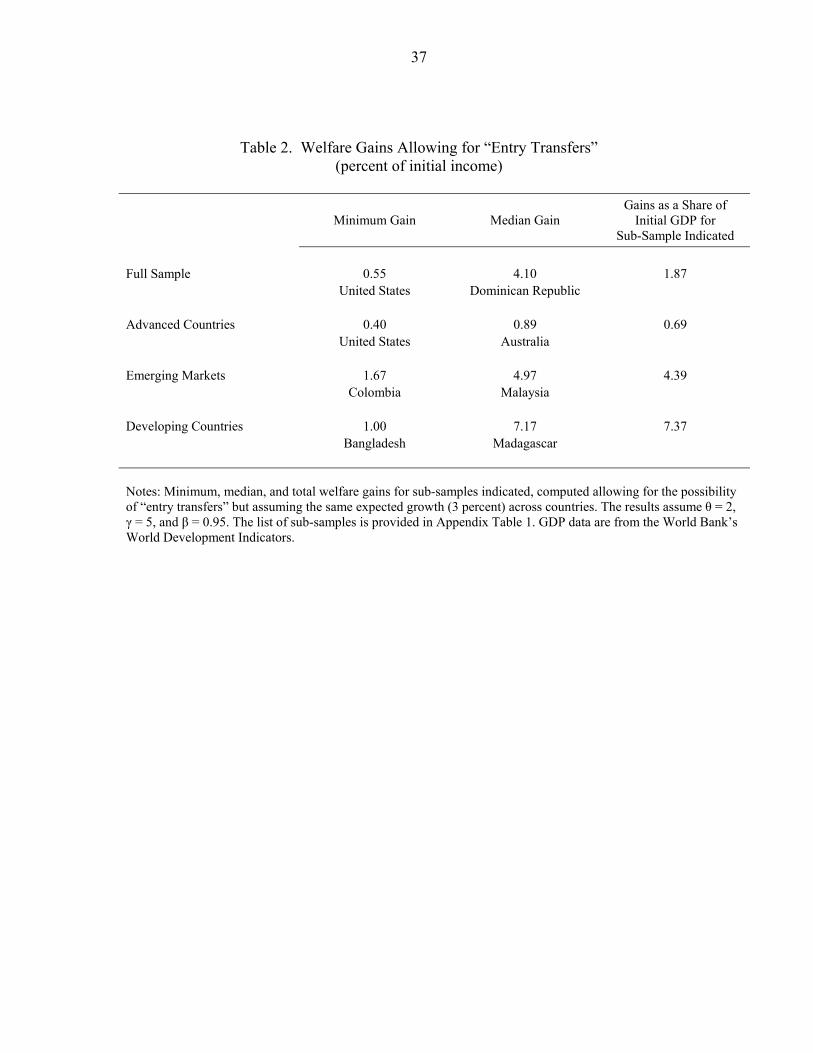
37
Table 2. Welfare Gains Allowing for “Entry Transfers” (percent of initial income)
Minimum Gain Median Gain
Gains as a Share of Initial GDP for
Sub-Sample Indicated Full Sample 0.55 4.10 1.87 United States Dominican Republic Advanced Countries 0.40 0.89 0.69 United States Australia Emerging Markets 1.67 4.97 4.39 Colombia Malaysia Developing Countries 1.00 7.17 7.37 Bangladesh Madagascar Notes: Minimum, median, and total welfare gains for sub-samples indicated, computed allowing for the possibility of “entry transfers” but assuming the same expected growth (3 percent) across countries. The results assume θ = 2, γ = 5, and β = 0.95. The list of sub-samples is provided in Appendix Table 1. GDP data are from the World Bank’s World Development Indicators.

38
Table 3. Gains from Risk Pooling Among Countries
(1) (2) (3) (4)
σ Individual Country Alone
σ Best Pool of
Any Size
δ Best Pool of
Any Size
Total Income-
Weighted Sum of Gains
All Countries (Pooling with any country)
3.62
0.54
3.88
1.87
Interest in Risk Sharing, by Level of Development, Size
Advanced (pooling with any country) 2.01 0.62 1.05 0.79 Advanced (pooling only with advanced) 2.01 0.89 0.86 0.69 Emerging (pooling with any country) 4.01 0.61 5.22 4.61 Emerging (pooling only with emerging) 4.01 1.07 4.65 4.39 Developing (pooling with any country) 5.15 0.51 9.14 8.04 Developing (pooling with only developing) 5.15 1.01 8.16 7.37 Small Countries (pooling with any country) 4.50 0.51 6.29 5.81 Small Countries (pooling only with small countries) 4.50 0.87 6.13 5.56
Current Degree of International Financial Integration High Integration Countries (pooling with any country) 2.61 0.61 1.94 1.32 High Integration Countries (pooling only with high integration countries) 2.61 0.74 1.84 1.30 Low Integration Countries (pooling with any country) 4.36 0.51 5.83 4.58 Low Integration Countries (pooling only with low integration countries) 4.36 0.76 5.55 4.21
Costs of Weak Enforcement Excellent Enforceability Countries (pooling with any country) 2.11 0.61 1.17 0.85 Below Excellent Enforceability Countries (pooling with any country) 4.41 0.52 5.90 5.12 Excellent Enforceability Countries (pooling only with excellent enforceability countries)
2.11 0.87 1.03 0.76
Emerging and Developing Country Excellent Enforceability (pooling with any excellent enforceability)
4.08 0.87 4.94 2.98
Emerging and Developing Excellent Enforceability (pooling only with emerging and developing excellent enforceability )
4.08 2.25 n.a. 1.52
Above Average Institutional Quality (pooling with any country) 2.61 0.61 1.94 1.06 Below Average Institutional Quality (pooling with any country) 4.26 0.52 5.32 5.42 Above Average Institutional Quality (pooling only with above average institutional quality countries)
2.61 0.82 1.74 0.99
Above Average Institutional Quality Emerging and Developing (pooling with any above average institutional quality country)
4.38 0.59 5.53 3.59
Above Average Institutional Emerging and Developing (pooling only with above average institutional quality emerging and developing)
4.38 1.64 5.08 2.83
Costs of Regional Constraints European Union (pooling only with advanced) 1.84 0.89 0.75 0.77 European Union (pooling only with EU) 1.84 1.05 0.68 0.55 Asian Emerging (pooling only with emerging) 3.62 1.09 3.60 3.54 Asian Emerging (pooling only with Asian emerging) 3.62 1.84 2.98 2.94 Latin American Emerging (pooling only with emerging) 4.41 1.07 5.73 5.39 Latin American Emerging (pooling only with Latin American emerging) 4.41 1.90 4.96 4.08
Notes: Column (1) reports the median (across countries in the indicated sub-sample) standard deviation of individual country growth. Column (2) reports the median (across countries in the indicated sub-sample) of the lowest possible standard deviation of poolwide growth. Column (3) reports the median welfare gain (across countries in the indicated sub-sample) obtained by entering the best possible pool of any size chosen within the indicated sub-sample without the possibility of entry transfers, and with pool and individual country growth rates assumed to be fixed at 3 percent per annum. Column (4) reports the income-weighted sum of welfare gains generated by a pool of all countries in the sub-sample, expressed as a share of total initial income for the indicated sub-sample with the possibility of entry transfers, and with pool and individual country growth assumed to be fixed at three percent per annum.
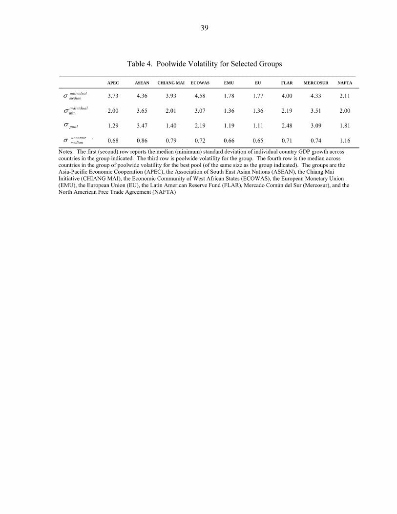
39
Table 4. Poolwide Volatility for Selected Groups
____________________________________________________________________________ APEC ASEAN CHIANG MAI ECOWAS EMU EU FLAR MERCOSUR NAFTA
3.73 4.36 3.93 4.58 1.78 1.77 4.00 4.33 2.11
2.00 3.65 2.01 3.07 1.36 1.36 2.19 3.51 2.00
1.29 3.47 1.40 2.19 1.19 1.11 2.48 3.09 1.81
0.68 0.86 0.79 0.72 0.66 0.65 0.71 0.74 1.16
poolσ
.unconstrmedianσ
individualmedianσ
individualminσ
Notes: The first (second) row reports the median (minimum) standard deviation of individual country GDP growth across countries in the group indicated. The third row is poolwide volatility for the group. The fourth row is the median across countries in the group of poolwide volatility for the best pool (of the same size as the group indicated). The groups are the Asia-Pacific Economic Cooperation (APEC), the Association of South East Asian Nations (ASEAN), the Chiang Mai Initiative (CHIANG MAI), the Economic Community of West African States (ECOWAS), the European Monetary Union (EMU), the European Union (EU), the Latin American Reserve Fund (FLAR), Mercado Común del Sur (Mercosur), and the North American Free Trade Agreement (NAFTA)
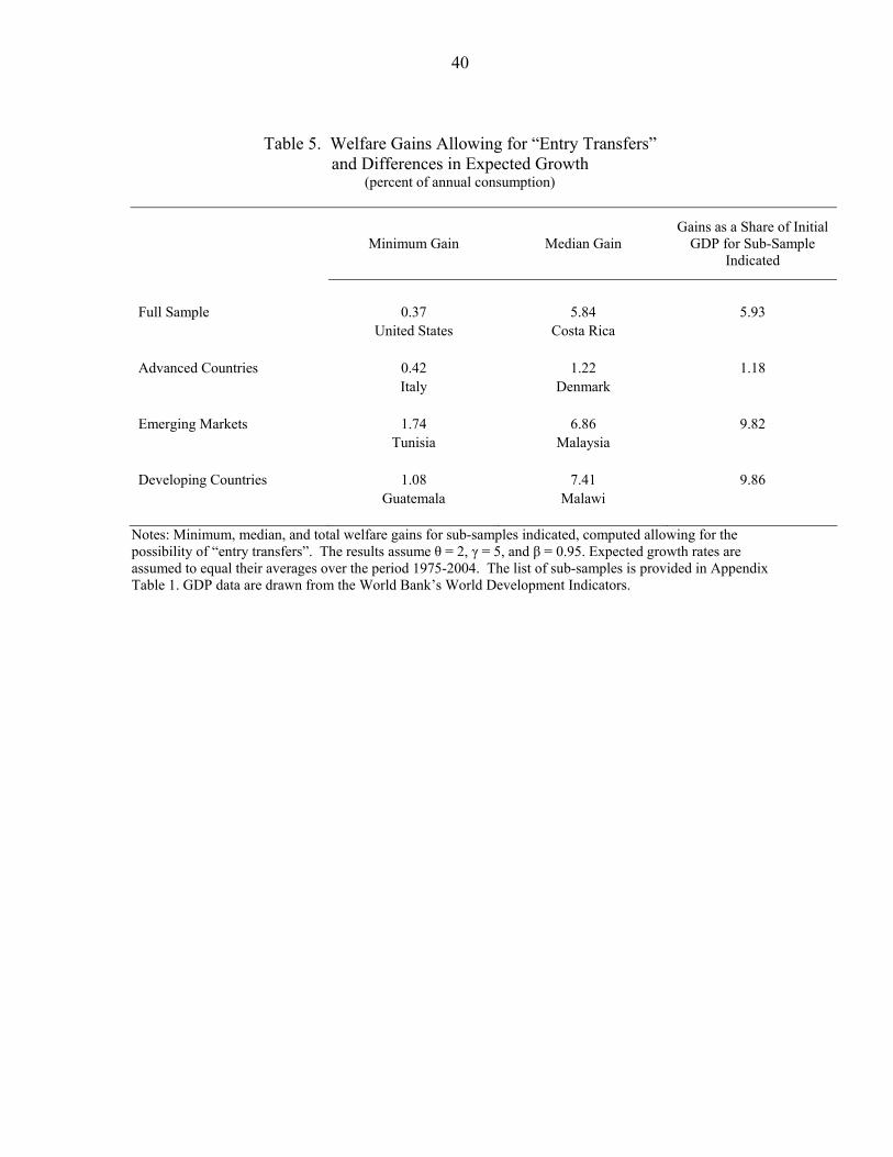
40
Table 5. Welfare Gains Allowing for “Entry Transfers”
and Differences in Expected Growth (percent of annual consumption)
Minimum Gain Median Gain Gains as a Share of Initial
GDP for Sub-Sample Indicated
Full Sample 0.37 5.84 5.93 United States Costa Rica Advanced Countries 0.42 1.22 1.18 Italy Denmark Emerging Markets 1.74 6.86 9.82 Tunisia Malaysia Developing Countries 1.08 7.41 9.86 Guatemala Malawi
Notes: Minimum, median, and total welfare gains for sub-samples indicated, computed allowing for the possibility of “entry transfers”. The results assume θ = 2, γ = 5, and β = 0.95. Expected growth rates are assumed to equal their averages over the period 1975-2004. The list of sub-samples is provided in Appendix Table 1. GDP data are drawn from the World Bank’s World Development Indicators.
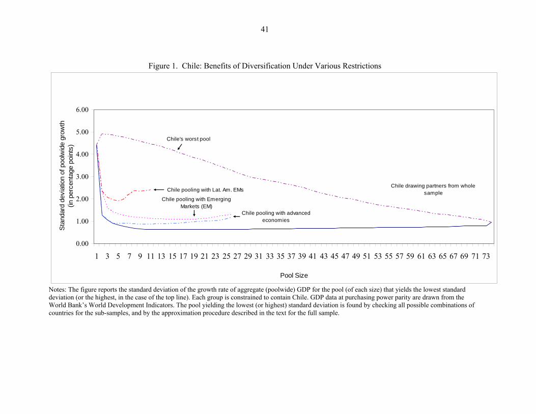
41
Figure 1. Chile: Benefits of Diversification Under Various Restrictions
Chile drawing partners from whole sample
Chile pooling with Emerging Markets (EM)
Chile pooling with Lat. Am. EMs
Chile pooling with advanced economies
Chile's worst pool
0.00
1.00
2.00
3.00
4.00
5.00
6.00
1 3 5 7 9 11 13 15 17 19 21 23 25 27 29 31 33 35 37 39 41 43 45 47 49 51 53 55 57 59 61 63 65 67 69 71 73
Pool Size
Sta
ndar
d de
viat
ion
of p
oolw
ide
grow
th(in
per
cent
age
poin
ts)
Notes: The figure reports the standard deviation of the growth rate of aggregate (poolwide) GDP for the pool (of each size) that yields the lowest standard deviation (or the highest, in the case of the top line). Each group is constrained to contain Chile. GDP data at purchasing power parity are drawn from the World Bank’s World Development Indicators. The pool yielding the lowest (or highest) standard deviation is found by checking all possible combinations of countries for the sub-samples, and by the approximation procedure described in the text for the full sample.

42
Figure 2. Is Chile’s Minimum Volatility Pool Stable?
Bangladesh
Group Size = 20(minimum volatility pool for
Chile)
Chile
0.50
0.55
0.60
0.65
0.70
0.75
0.80
1 3 5 7 9 11 13 15 17 19 21 23 25 27 29 31 33 35 37 39 41 43 45 47 49 51 53 55 57 59 61 63 65 67 69 71 73
Pool Size
Stan
dard
dev
iatio
n of
poo
lwid
e gr
owth
(in
per
cent
age
poin
ts)
'Austria''Bangladesh''Benin''Botswana''Cameroon''Chile''CongoRepublic of''CostaRica''DominicanRepublic''ElSalvador''Gambia''Iceland''Kenya''Lesotho''NewZealand''Nicaragua''Senegal''Sweden''SyrianArabRepublic''Zimbabwe'
Notes: The line corresponding to each country represents the lowest possible standard deviation of poolwide growth for pools that include the country in question, for each pool size. GDP data are from the World Bank’s World Development Indicators.

43
Figure 3. Lowest Poolwide Volatility Envelopes for Samples Constrained by Level of Development
Global envelope
Advanced
EmergingDeveloping
0
0.5
1
1.5
2
2.5
1 4 7 10 13 16 19 22 25 28 31 34 37 40 43 46 49 52 55 58 61 64 67 70 73
Pool Size
Stan
dard
dev
iatio
n of
poo
lwid
e gr
owth
(in
per
cent
age
poin
ts)
Notes: The figure reports the standard deviation of the growth rate of poolwide GDP for the pool (of each size) that yields the lowest standard deviation for each indicated sub-sample. The pool yielding the lowest standard deviation is found by checking all possible combinations of countries for the sub-samples, and by the approximation procedure described in the text for the full sample. GDP data are from the World Bank’s World Development Indicators.

44
Figure 4. Pooling Gains
Developing Countries
Emerging Markets
Advanced Countries
Full Sample
0.0
1.0
2.0
3.0
4.0
5.0
6.0
7.0
8.0
1 4 7 10 13 16 19 22 25 28 31 34 37 40 43 46 49 52 55 58 61 64 67 70 73Pool Size
Tota
l wel
fare
gai
ns o
f (su
b-) u
nive
rse
(per
cent
of c
onsu
mpt
ion)
Notes: For each pool size, the figure reports the highest possible (income-weighted) sum of welfare gains obtained by pool members compared with the status quo (“autarky”), scaled by aggregate GDP of the (sub-)universe of countries in question (as indicated). The welfare gains are computed allowing for “entry transfer” payments as in Lewis (2000). The results assume θ=2, γ=5, and β=0.95 and a constant growth rate of three percent for all countries and pools. GDP data are from the World Bank’s World Development Indicators.

45
Figure 5. Trade and Diversification Benefits
.85 1 1.2 1.4 1.6 1.8 2 0
2
4
6
8
10
12
Standard deviation of poolw ide grow th (percentage points)
Tra
de in
tegr
atio
n (p
erce
nt o
f GD
P) Advanced Countries (P=5)
.85 1 1.2 1.4 1.6 1.8 2 0
2
4
6
8
10
12
Standard deviation of poolw ide grow th (percentage points)
Tra
de in
tegr
atio
n (p
erce
nt o
f GD
P) Advanced Countries (P=10)
.85 1 1.2 1.4 1.6 1.8 2 0
2
4
6
8
10
12
Standard deviation of poolw ide grow th (percentage points)T
rade
inte
grat
ion
(per
cent
of G
DP
) Emerging Markets (P=10)
.85 1 1.2 1.4 1.6 1.8 2 0
2
4
6
8
10
12
Standard deviation of poolw ide grow th (percentage points)
Tra
de in
tegr
atio
n (p
erce
nt o
f GD
P) Developing Countries (P=510)
.85 1.0 1.2 1.4 1.6 1.8 2 0
2
4
6
8
10
12
Standard deviation of poolw ide grow th (percentage points)
Tra
de in
tegr
atio
n (p
erce
nt o
f GD
P) Emerging Markets (P=5)
.85 1.0 1.2 1.4 1.6 1.8 2 0
2
4
6
8
10
12
Standard deviation of poolw ide grow th (percentage points)
Tra
de in
tegr
atio
n (p
erce
nt o
f GD
P) Developing Countries (P=5)
Notes: The scatter plots report poolwide trade integration and the standard deviation of the growth rate of aggregate (poolwide) GDP for all pools of sizes 5 and 10 (as indicated) drawn from the sub-samples indicated. Trade integration is the sum (across pool members) of exports to other pool members, divided by poolwide GDP. To compute trade integration, the data on exports (in US$ at current prices) are from the International Monetary Fund’s Direction of Trade Statistics, and the data on GDP (in US$ at current prices) are from the IMF’s World Economic Outlook database. To compute growth volatility, GDP data (PPP) are from the World Bank’s World Development Indicators.

46
Figure 6: Pooling Gains Allowing for Differences in Expected Growth
Developing Countries
Emerging Markets
Advanced Countries
Full Sample
0.0
2.0
4.0
6.0
8.0
10.0
12.0
1 4 7 10 13 16 19 22 25 28 31 34 37 40 43 46 49 52 55 58 61 64 67 70 73Pool Size
Tota
l wel
fare
gai
ns o
f (su
b-) u
nive
rse
(per
cent
of c
onsu
mpt
ion)
Notes: For each pool size, the figure reports the highest possible (income-weighted) sum of welfare gains obtained by pool members compared with the status quo (“autarky”), scaled by aggregate GDP of the (sub-)universe of countries in question (as indicated). The welfare gains are computed allowing for “entry transfer” payments as in Lewis (2000). The results assume θ=2, γ=5, and β=0.95 and a observed average growth rates. GDP data are from the World Bank’s World Development Indicator.