Polynomial-Time Quantum Algorithms for Pell’sEquation and the Principal Ideal Problem∗

Sean Hallgren†

NEC Laboratories America, Inc.4 Independence WayPrinceton, NJ 08540

hallgren@nec-labs.com

May 9, 2006

Abstract

We give polynomial-time quantum algorithms for three problems from computa-tional algebraic number theory. The first is Pell’s equation. Given a positive non-square integer d, Pell’s equation is x2 − dy2 = 1 and the goal is to find its integersolutions. Factoring integers reduces to finding integer solutions of Pell’s equation, buta reduction in the other direction is not known and appears more difficult. The secondproblem we solve is the principal ideal problem in real quadratic number fields. Thisproblem, which is at least as hard as solving Pell’s equation, is the one-way functionunderlying the Buchmann-Williams key exchange system, which is therefore broken byour quantum algorithm. Finally, assuming the generalized Riemann hypothesis, thisalgorithm can be used to compute the class group of a real quadratic number field.

1 Introduction

The search for quantum algorithms is a fundamental goal of quantum computing, and thereis a great deal of interest in how quantum computing changes the tractable-intractableboundary in polynomial-time computation. Shor’s algorithms [Sho97] for factoring anddiscrete log resulted in much excitement over the potential of quantum computation. At

∗A preliminary version of this paper appeared in STOC’02 [Hal02]. Work done at MSRI, U.C. Berkeley,and Caltech.

†Supported at Caltech in part by an NSF Mathematical Sciences Postdoctoral Fellowship, NSF throughCaltech’s Institute for Quantum Information, NSF under grant no. 0049092 (previously 9876172) and TheCharles Lee Powell Foundation. Part of this work done while the author was at MSRI and U.C. Berkeley,with partial support from DARPA QUIST Agreement No. F30602-01-2-0524.

1

the same time it also showed that current methods of cryptography used on the In-ternet will have to be changed if quantum computers can be built. Since Shor’s algo-rithms, much work has gone into a generalized problem called the hidden subgroup prob-lem [EHK99, HRTS00, GSVV01, FIM+03, Kup03, MRRS04]. This problem includes asspecial cases previously solved problems such as factoring and discrete log, as well as stillunsolved problems such as graph isomorphism. While progress has been made on the hid-den subgroup problem, finding more problems where quantum computation has a significantadvantage over classical computation has been difficult [Sho03].

In this paper, we give polynomial-time quantum algorithms for Pell’s equation and theprincipal ideal problem. Using these algorithms, we are also able to compute the classgroup of a real quadratic number field, and break, when given a quantum computer, the keyexchange protocol proposed by Buchmann and Williams [BW89a]. Besides giving natural,well-studied examples, this paper extends the hidden subgroup framework and points towardshow to extend it further. This provides insights into the nature of Fourier sampling, the mainworkhorse of quantum algorithms. In particular, while the hidden subgroup problem can bedefined over any group, Fourier sampling can only be performed over finite groups. One canview Shor’s work as showing how to effectively use Fourier sampling when then underlyinggroup is finitely generated. In this work we extend Fourier sampling to non-finitely generatedgroups, as there will be an underlying periodic function over the reals whose period we wishto approximate.

We also shed light on what cryptography might look like if quantum computers can bebuilt. It is known that the current systems which assume factoring is computationally hardwill be broken by quantum computers. Here we show that a potentially much more securesystem can be broken too.

Pell’s equation is one of the oldest problems studied in number theory. Given a positivenon-square integer d, Pell’s equation is x2 − dy2 = 1, and the goal is to find all integersolutions. The original algorithm for solving it is the second oldest number theory algorithmafter Euclid’s algorithm. The algorithm is due to Indian mathematicians around 1000 a.d.In 1768 Lagrange showed that there are an infinite number of solutions of the equation, andthe following theorem is well-known. If (x1, y1) is the least positive solution of x2 − dy2 = 1,ordered by the value of x1 + y1

√d, where d is a positive non-square integer, then all positive

solutions are given by (xn, yn) for n = 1, 2, 3, . . ., where xn + yn

√d = (x1 + y1

√d)n [NZM91].

It is not actually possible to have a polynomial-time algorithm for finding the leastpositive solution (x1, y1), because it may take exponentially many bits to represent (the inputsize is log d). Instead, the integer closest to the regulator, defined as R = ln(x1 + y1

√d), is

computed. Given this integer bRe it is possible to compute R to arbitrary precision, andbRe uniquely identifies (x1, y1). In fact, it is enough to solve a closely related problem, whichis finding the regulator of the ring Z[

√d]. This is the problem we solve, described precisely

in the next section. We also solve another problem related to the ring Z[√

d], called theprincipal ideal problem. The principal ideal problem is the following: given an invertibleideal I determine if there exists an α ∈ Q(

√d) such that I = αZ[

√d], and if there is,

find α. As with Pell’s equation this value may be too large, but finding the closest integerto log α is enough to uniquely identify α. Using our quantum algorithm for this problemand assuming the GRH, we can also compute the class group of a real quadratic number

2

field. Full definitions will be given in the next section. For more about Pell’s equation,see [Wil00, Len02].

The expected running time of the classical algorithms for these problems is measured us-ing the function L(a, b) = exp(bna(log n)1−a), where n is the input size. The goal is to reducea to zero, which would be polynomial-time. The best algorithm for factoring integers has ex-pected time L(1

3, b) for some constant b [LL93]. Assuming the GRH, the best algorithms for

Pell’s equation and the principal ideal problem have expected time L(12, b′) [Buc89, Vol00],

for some constant b′, so there is an sub-exponential gap between the best known classicalalgorithms. Both the running time and the correctness of the classical algorithm for Pell’sequation are based on the generalized Riemann hypothesis (GRH). The GRH appears inmany algorithms in number theory and is used sometimes to show correctness and sometimesto analyze the running time. For example, the best classical algorithm for Pell’s equationwithout assumptions is O(d1/4polylog d). In addition, while finding multiples of the regulatoris in NP, finding the regulator itself is only known to be in NP under the GRH [BW89a]. Ourquantum algorithms for computing the regulator (solving Pell’s equation) and the principalideal problem do not use any assumptions.

There are reductions from factoring to solving Pell’s equation, and from solving Pell’sequation to solving the principal ideal problem [BW89b]. However, Pell’s equation and theprincipal ideal problem appear to be harder than factoring, and there are no reductionsknown in the other direction. This is reflected in the gap between the running times ofthe best algorithms for factoring and Pell’s equation. Indeed, a key exchange system basedon the principal ideal problem is proposed in [BW89b], and one of the motivations is thateven if there turns out to be a polynomial-time algorithm for factoring, their system mightstill be unbreakable. Our quantum algorithm for the principal ideal problem breaks this keyexchange system in this context.

Classically, computing the class group appears to be computationally tied to computingthe regulator [Coh93], or in other words, there is no reason to compute one without theother. Curiously, this does not appear to be the case with respect to quantum algorithms.The primary problem we must overcome to compute the class group is the fact that groupelements do not have unique representatives. Furthermore, the structure of the represen-tatives is arbitrary, making techniques in [Wat01] inapplicable. To deal with this problemour algorithm must first compute the regulator, and then use the principal ideal problemalgorithm as a subroutine to create superpositions over equivalence classes.

The quantum step in our algorithm for Pell’s equation is a new procedure to efficientlyapproximate the period of a periodic function with irrational period. The algorithm for theprincipal ideal problem reduces to a discrete log type problem, but there is no longer anunderlying group. Instead, a group-like subset of the reals modulo an irrational number isused. This prevents direct application of Shor’s algorithms. Dealing with these problems,and the one for the class group, are the main technical pieces of the paper.

2 Background

We will use the following notation: a, b, c, d, i, j, k, l, m, n, p, q, N are non-negative integers,x, y, z, R, S are real numbers, and f , g, h are functions. When computing with real numbers

3

we mean computing with approximations that are good enough for our purposes.

2.1 Quantum Computing Background

All problems that have quantum algorithms with superpolynomial or exponential speedupsover the best known classical algorithm have quantum algorithms that use Fourier sam-pling [BV97]. Given a quantum state, Fourier sampling is the process of computing theFourier transform and measuring the result. This primitive differs in two important waysfrom just computing the classical Fourier transform of a vector. First, the quantum Fouriertransform can be computed exponentially faster. In the current context this means it canbe computed in polynomial-time even though the state vector has exponential size. Sec-ond, the output of the primitive is not a vector of complex numbers, but only a clas-sical bit string. A string is measured with probability equal to its amplitude squared.Thus, the phases are ignored, and there is far more restricted access to the output vec-tor from the Fourier transform than in the classical case. Except for the problems solvedin [vDHI03], it is sufficient to use the stronger primitive of Fourier sampling a function (forexample [Sim97, Sho97, HRTS00, GSVV01, IMS01]).

Given a function f , Fourier sampling the function f is the process of creating the super-position 1√

|G|

∑g∈G |g, f(g)〉, optionally measuring the second register containing f(g) (or

just creating 1√|G|

∑g∈G f(g)|g〉 in the case of [BV97]), and then Fourier sampling.

The most common application of Fourier sampling is the Hidden Subgroup Problem. Inthis problem a group G and a function f : G → S are given with the condition that thereis an unknown subgroup H ≤ G such that the function f is constant on (left) cosets of H,and takes different values on different cosets. The task is to find a set of generators for H.The range of f is a set S. Fourier sampling the function f in this case first creates a statethat is uniform on a coset of the subgroup H ≤ G: 1√

|H|

∑h∈H |g + h〉, where g is chosen

uniformly from G and f(g) was the value measured in the second register. The second stepcomputes the Fourier transform over G and measures. In this approach the hidden subgroupfunction is only used to set up a superposition which is essentially a characteristic functionof a random coset.

For example, for the hidden subgroup problem over the finite cyclic group Zrm =0, 1, 2, . . . , rm − 1 with hidden subgroup Zr = 0, m, 2m, . . . , (r − 1)m, the Fouriertransform “inverts” the period, and the resulting distribution is uniform over the pointsof Zm = 0, r, 2r, . . . , (m − 1)r. Sampling from this distribution allows one to compute r,and from r, the generator m. Shor’s algorithm extends this idea to the infinite group Z, byFourier sampling f over a large enough cyclic subgroup Zq. In that case, for a subgroupH = 〈m〉, samples will be concentrated around integer multiples of q/m. In this paper weextend this further to the case of G = R, where H can be generated by an irrational number.

One of the properties that makes Fourier sampling useful in the hidden subgroup problemis that the resulting distribution is independent of the coset. This can be seen from theconvolution-multiplication property of the Fourier transform. Fourier sampling

∑s∈S cS|s〉,

where S is a subset of some abelian group with addition and cS = 1√|S|

, is the same as

Fourier sampling∑

s∈S cS|k + s〉, where k is a group element. We see that F (∑

s cS|k +

4

s〉) = F (|k〉 ∗∑

s cS|s〉) = (F |k〉) · (F∑

s cS|s〉), where ∗ is convolution and · is point-wisemultiplication. Here F |k〉 is the Fourier transform of the delta function |k〉, and is uniformin magnitude, so the distribution is determined only by F

∑s cS|s〉.

The other property used is that the Fourier transform of a state that is uniform over anormal subgroup of a finite group is uniform over representations that contain the subgroupin their kernel [HRTS00]. The subgroup can then be computed (efficiently when the groupis abelian) from polynomially many samples.

In our algorithms we will use the first property and prove a new generalization of thesecond property.

2.2 Algebraic Number Theory Background

This section is intended to give a short overview of the background and the objects thatappear. An introduction to the subject when d is assumed to be square-free can be foundin [Joz03]. For the general non-square case, background can also be found in [BTW95,Len82b, Coh93].

The integer d is the input to our algorithm so the input size is log d, and by “polynomial-time” we mean polynomial in log d.

For a positive non-square integer ∆, K = Q(√

∆) is called a real quadratic number field.It is the set of numbers u + v

√∆ : u, v ∈ Q and it is a field. When ∆ is also congruent

to 0 or 1 modulo 4 it is called a quadratic discriminant, and the order O of discriminant

∆ is the subring O = Z[∆+√

∆2

] ⊆ K. It consists of the elements a + b∆+√

∆2

: a, b ∈ Z,and each α ∈ O has a unique representation as α = a+b

√∆

2, where a, b ∈ Z. The norm of

an element a+b√

∆2

is defined by a+b√

∆2

· a−b√

∆2

= a2−b2∆4

. The units of O are the invertibleelements in O. They have norm ±1 and have the form ±εk, where k ∈ Z, and ε is called afundamental unit. The fundamental unit can be chosen so that ε > 1 and with that choicethe regulator of O is defined to be R = ln ε. The fundamental unit in this representationcan have exponentially many bits, so more compact representations, such as bRe, the closestinteger to the regulator of O, are computed. The regulator satisfies R ≤

√∆ log ∆ [Len82a],

so bRe requires only a number bits which is polynomial in log ∆ to represent. We will showhow to compute bRe, in quantum polynomial-time.

To solve Pell’s equation, given an algorithm to compute bRe when given an order, weproceed as follows. Given an instance d of Pell’s equation, compute bRe of the order withdiscriminant ∆ = 4d, which satisfies O = Z[

√d]. Let x0, y0 be such that ε = eR = x0 +y0

√d

is the fundamental unit of O. Then the norm of ε is (x0+√

dy0)(x0−√

dy0) = x20−dy2

0 = ±1.To be a solution of Pell’s equation we need to restrict to the norm one case. Even thoughthe norm equation involves numbers potentially to large to compute with in polynomial-time it is possible to compute the norm in polynomial time from bRe. This can be doneby first computing R to a higher precision using classical algorithms (discussed below), andcomputing the compact representations and using the norm algorithm of [BTW95, Theorem5.5]. If the computed norm is 1, then bRe is the solution to Pell’s equation since x2

0−dy20 = 1.

If the norm is −1, then using the fact that norm is multiplicative, ε2 generates the solutionsof Pell’s equation, so 2R is the solution which can be computed to high precision from bReusing classical algorithms.

5

Next we discuss how to gain access to information about the regulator R given an orderO. The product of two subsets I, J ⊆ K is the additive subgroup of K generated byxy : x ∈ I, y ∈ J. An invertible O-ideal I is a subset of K such that OI = I and forwhich there exists a subset J ⊆ K with IJ = O. The set of invertible ideals of O form anabelian group under multiplication and will be denoted I. A principal ideal I is an additivesubgroup of K of the form Oα, with α ∈ K. The set of principal ideals will be denotedP , and it is a subgroup of I. Finally, we need the set of reduced ideals R. Let xZ + yZdenote the set xa + yb : a, b ∈ Z. Let τ(b, a) denote the unique integer τ such that τ ≡ bmod 2a,−a < τ ≤ a if a >

√∆, and

√∆− 2a < τ <

√∆ if a <

√∆. An invertible ideal I

has the form

I =m

l

(aZ +

b +√

∆

2Z

)(1),

where l ∈ N, a, b,m ∈ Z, a,m > 0, b = τ(b, a), and 4a divides ∆− b2 [BTW95]. An ideal I isreduced when 1 is a minimum in the ideal, which is a technical condition defined in [BTW95].When an ideal is reduced, m = 1 and a = l. Furthermore, a, |b| <

√∆. It follows that R is

finite and has at most 2∆ elements. R is not a group, but is group-like under multiplication(as defined below).

The distance function δ : P → R/RZ is defined by δ((u + v√

∆)O) = 12ln∣∣∣u+v

√∆

u−v√

∆

∣∣∣ mod

R [Len82b]. The unit ideal O has distance δ(1 · O) = 12| ln 1| = 0. The function is well

defined since for a unit ε, δ(εO) = 12

∣∣ln εε−1

∣∣ = 12|ln ε2| = 0 mod R. The class group is the

finite abelian group Cl = I/P . It provides a measure of how far O is from being a principalideal domain (PID), in the sense that it O is a PID if and only if Cl is trivial.

The main two operations performed on I are composition (·) and reduction (ρ). Thereis also an operation which combines the two called multiplication (∗). It is not known howto compute the distance between two ideals in polynomial time if they are given in standardrepresentation (1), (this would solve the principal ideal problem), but given an ideal I, itis possible to compute the distance to a new ideal J , without reduction modulo R which isunknown, if J is computed from I using composition and reduction. In particular, if thedistance of I from O is known, and J is computed from I using composition and reduction,then the distance of J from O can be computed. These distances can be computed to a roughaccuracy, say the closest integer, and later computed to a greater precision. To achieve thisit is only necessary to keep track of the sequence of composition and reduction steps, and torun the same sequence of composition and reduction steps again using the higher precision.

The composition of two ideals I, J ∈ I is their product I · J ∈ I. The distance functionsatisfies δ(I ·J) = δ(I)+δ(J). Reduction is a map from I to I, and after a polynomial numberof steps, the ideal will be in R (reduced). We will not give the formula for the reduction stephere, but δ(I)+ 1√

∆≤ δ(ρ(I)) ≤ δ(I)+ 1

2ln ∆. Also, two applications has a constant minimum

distance: δ(ρ2(I)) > δ(I) + ln 2. The effect of reduction on I is to multiply it by an elementin K, so reduction preserves the ideal class, i.e. the member of the class group. Multiplication∗ : R → R takes reduced ideals I, J , and I ∗ J is computed by first applying composition,and then applying reduction a polynomial number times k until it is reduced. Thereforeδ(I ∗J) = δ(ρk(I ·J)) = δ(I ·J)+(δ(ρk(I ·J))−δ(I ·J)) = δ(I)+δ(J)+(δ(ρk(I ·J))−δ(I ·J)).The last term is at most a polynomial and it is in this sense that R is group-like. If the last

6

term was zero, then distances would add, and δ would be a homomorphism on R. However,it is only true that δ is a homomorphism on I. Also, multiplication of two elements in R iscommutative but not associative.

The reduction step ρ restricted to R is a permutation, and the equivalence class moduloP is preserved (e.g. a principal ideal stays principal) after application. In fact, it is possibleto cycle through the set of all reduced principal ideals, called the principal cycle, by pickingone and applying powers of ρ to it. This is also true for any set of reduced ideals modulo P .

Algorithm 2.1 (Computing a reduced ideal to the left of x).Input: A rational number x.Output: The reduced ideal I to the left of or at x mod R and its distance to x.

1. Apply ρ twice to O to compute an ideal I ′ and its distance δ(I ′). The distance δ(I ′) isat least a constant and at most a polynomial in log ∆.

2. Use repeated squaring of the operation ∗ to compute an ideal I ′′ within a polynomialdistance of x and its distance δ′′ to x.

3. Use ρ to search the region for the appropriate ideal I and its distance δ to x.

The distance is kept at some chosen precision. Since any pair of ideals is separated by atleast 1/

√∆, a polynomial number of precision bits suffices for distinguishing different ideals.

For any ideal J , principal or not, and distance x ∈ Q, the ideal J ′ that is x away from J canalso be computed in a similar manner: first compute the ideal I at distance x from O, andthen multiply J and I.

When computing the ideal to the left of or at x, a technical problem arises when the idealhas a distance too close to x and the precision used cannot distinguish whether the ideal isto the left or right of x. The third part of the next definition handles this problem.

The main functions we are interested in are the following:

Definition 2.1. Let Ix be the reduced the ideal to the left of or at x. More generally, givena reduced ideal J and a distance x, let IJ,x be the ideal at the largest distance less than orequal to x from J .

1. Define f : R → I × R by f(x) = (Ix, δx), where δx = x− δ(Ix).

2. Define fJ : R → I × R by fJ(x) = (IJ,x, δJ,x), where δJ,x = x− δ(I−1J).

3. Let j, L ∈ Z. Define fJ,j : R → I × R by fJ,j(x) = (IJ,x+j/L, δJ,x+j/L).

The first type of function is used, for example, in [BW89b]. The first function is a specialcase of the second one since f = fO. The second function is a special case of the third onesince fJ = fJ,0. The function f is one-to-one in [0, R), and has period R, the regulator.It is well-defined, and therefore one-to-one in [0, R), because the distance between any tworeduced ideals is positive. It has period R because the distance function is defined moduloR. For example, applying the reduction step to the ideal with greatest distance modulo Rresults in the unit ideal, and the function repeats. The function fJ,j has the same properties,it is simply takes f and shifts it by the ideal J and by the distance j/L.

7

We will need to work with discretized versions of f and this is done by restricting thedomain to the integers or rational numbers, and by computing the distance δ to some desiredprecision. One technical problem which arises is that conceivably an ideal has a distance soclose to x that the precision used in the algorithm cannot determine if the ideal is on theleft or right of x. In general there is no known upper bound on the precision to preventthis from happening. The result can be that an algorithm which tries to compute f ontwo different inputs incorrectly returns the same value. For example, consider an algorithmwhich attempts to compute f(i/N) and f((i + 1)/N). If different repeated squaring stepsare used and the rounding is different as a result, then the algorithm could return (I, 0) forboth, even though the function values differ.

The precision problem can be fixed using fJ,j. If fJ,j is evaluated on integer multiples of1/N and no ideal is close to an evaluation point i/N then there are no problems.

Claim 2.1. Let N, q ∈ Z, L = qN16. With probability 1 − 1/N over choices of j ∈0, . . . , L/N − 1, if i ∈ 0, . . . , q − 1 then no reduced ideal is within 1/L of i/N + j/L.

Proof. Limiting the domain to [0, q/N ] upper bounds the number of reduced ideals encoun-tered to q/N ·2/ ln 2 (including repeats). Because there are at at most q rational numbers i/Nand at most q/N ·2/ ln 2 reduced ideals, the probability that no ideal has a distance closer than1/L to one of the rational numbers i/N is at least 1−(q/N ·2/ ln 2)/((L/2)/N) ≥ 1−1/N .

It is possible to check if a given number x is within a polynomial distance of a multiple ofthe regulator. Given x, compute the ideal closest to it. Then apply ρ and ρ−1 a polynomialnumber of times and search for the unit ideal.

To summarize:

Theorem 1. Let O be an order of discriminant ∆. Given ∆, let N, a, b be integers whichare polynomial in ∆.

1. Let q, N ∈ Z, L = qN16, J be a reduced ideal, and fJ,j be as in Definition 2.1. Thenwith probability 1− 1/N over choices of j ∈ 0, . . . , L/N, fJ,j(i/N) can be evaluatedin time polynomial in log ∆ when i ∈ 0, . . . , q − 1.

2. For a distance u = a/b ∈ Q and a reduced ideal I, it is possible to check if u mod R iswithin a polynomial of the distance of I in time polynomial in log ∆. In particular, itis possible to efficiently check if a rational number is near a multiple of the regulator,by using the unit ideal O as I.

3 Computing the Regulator

In this section we develop an algorithm for computing the regulator. This will be done byfinding the period of a periodic function defined on the reals. In Section 3.1, we show how tofind the period of a function which is discrete but still has an irrational period. In Section 3.2we show how to construct such a function for the regulator.

8

3.1 Approximating Irrational Periods of Functions

Given a function with an irrational period, we must first discretize it to use it in an algorithm.We start by defining the notion of pseudo-periodic to handle this.

Definition 3.1. A function f : Z → X, where X is any set, is called pseudo-periodicwith period S, at offset k if for each i either f(k) = f(k + biSc) or f(k) = f(k + diSe),where S ∈ R. We write this condition as f(k) = f(k + [iS]) to denote either floor orceiling. A function is ε-pseudo-periodic with period S if for at least an ε-fraction of offsetsk ∈ 0, . . . , bSc, f is pseudo-periodic at offset k.

Given a periodic function f with period S ∈ Z which is also injective in 0, . . . , S−1 it iseasy to verify that an integer T is a multiple of the period by checking whether f(0) = f(T ).Given a function which is pseudo-periodic and injective on a subset of offsets for which itis pseudo-periodic, it is not quite as straightforward to verify the period. For the sake ofsimplicity we will assume there is an efficient way to check the period in the period findingalgorithm, as will exist in our application in Section 3.2.

Definition 3.2. A verification procedure for the period of a function with irrational periodas in Definition 3.1 returns yes when the input T is within one of S, or alternatively, whenT is within one of an integer multiple of S.

The idea of the algorithm for pseudo-periodic functions is the same as the original periodfinding algorithm: the Fourier transform inverts the period. In this case the superpositioncreated during Fourier sampling is no longer periodic but only pseudo-periodic. Followingthe general idea however, if we Fourier sample f over Zq and observe an integer c, thenc should be close to an integer multiple of the irrational number q/S, and from this wewill recover a value close to S. If computing with irrational numbers were possible, thengiven two random integer multiples kα and lα, the irrational number α can be computed bydividing the two numbers to get k/l, and then dividing kα by k. This idea works if k andl are relatively prime, which happens with inverse polynomial probability. Fourier samplingf actually results in rounded versions of kα and lα, but we will show that k/l will appearin the continued fraction expansion of the ratio of the two measured values.

Algorithm 3.1 (Approximate the period of a pseudo-periodic function).Input: An ε-pseudo-periodic function f with period S ∈ R such that if k1 and k2 are amongthe ε-fraction of pseudo-periodic offsets then f(k1) 6= f(k2), an efficient verification procedureas in Definition 3.2, and upper bound M on the period S.Output: An integer within one of S.

1. Choose an integer q ≥ 3M2.

2. Fourier sample f over Zq twice resulting in values c and d.

3. Compute the continued fraction expansion of c/d.

4. For each convergent ci/di, test whether bciq/ce is a multiple of the period.

9

5. Output the smallest value bciq/ce that was a multiple of the period in Step 4.

In the algorithm an upper bound on S is needed, however the standard method of cir-cumventing this can be used. Assume S is at most two and run the algorithm, if the answeris wrong, double the bound on S and repeat the algorithm. In a polynomial in log S numberof steps a correct bound will be used and the algorithm will return the correct answer.

Lemma 3.1. Given an ε-pseudo-periodic function with period S ∈ R greater than someabsolute constant such that if k1 and k2 are among the ε-fraction of pseudo-periodic offsetsthen f(k1) 6= f(k2), an efficient verification procedure for the period, and an upper bound Mon S, Algorithm 3.1 computes an integer a such that |S−a| ≤ 1 in time polynomial in log S,with probability Ω(ε2/(log M)4).

Proof. One Fourier sampling step starts by evaluating the function in superposition andmeasuring the function value. Suppose this results in measuring f(m), where m ≤ S. Sincef is pseudo-periodic at an ε fraction of offsets, with probability at least ε, f is pseudo-periodicat m. If f is not pseudo-periodic at m then the rest of the algorithm will be completed andsome integer will be returned, which will probably fail the verification procedure.

Let p = b(q−m)/Sc. If f is pseudo-periodic at offset m then the resulting superpositionis 1√

p

∑p−1i=0 |m + [iS]〉. Since we are Fourier sampling, we may assume w.l.o.g. that m = 0.

Therefore the measured distribution will be the same as the one induced by Fourier sampling1√p

∑p−1i=0 |[iS]〉.

The Fourier transform at |j〉 has amplitude 1√pq

∑p−1i=0 ω

j[iS]q . This is similar to a geometric

series except that each term iS rounded to [iS]. Let [iS] = iS + δi, where −1 < δi < 1. Let

j = k qS

+ ε, for k ∈ 0, . . . , bSc, and −12≤ ε ≤ 1

2. Then the fraction in the ω

j[iS]q term is

j[iS]

q=

(k

S+

ε

q

)(iS + δi) =

εiS

q+

kδi

S+

εδi

q(mod 1).

When j ≤ q/2 log M , |kδi/S| ≤ 1/2 log M and the rounding term in [iS] is |kδi/S| +|εδi/q| ≤ 2/ log M . The condition in Claim 3.1 states that iδ/M should be at most 3/4, andin the present case i ≤ q/S, so we have |εiS/q| ≤ 1/2. For p we have p = b q−m

Sc ≥ q/S−2 ≥

3M2/S − 2 ≥ 3M − 2. When M ≥ 2262 we can apply Claim 3.1,∣∣∣∣∣ 1√

pq

p−1∑i=0

ωj[iS]q

∣∣∣∣∣2

≥ 1

pqcp2,

where c is a constant. Then the probability of measuring an integer of the form bk qSe is at

least cp/q ≥ c/(2S).There are S/ log M integer multiples of q/S less than q/ log M so the probability of mea-

suring two values less than q/ log M is at least Ω(1/(log M)2). Furthermore, the probabilitythat the two values are relatively prime is at least Ω(1/(log(S/ log M))2) by the prime num-ber theorem. The probability of measuring two such values satisfying all the conditions istherefore at least Ω(ε2/(log M)4).

10

Given that c = bkq/Se and d = blq/Se, we now show that k/l is a convergent in thecontinued fraction expansion of c/d. We will use the fact that if x is any irrational number,a/b ∈ Q, and |x − a/b| ≤ 1

2b2, then a/b is a convergent in the continued fraction expansion

of x [Sch86]. We will show that | cd− k

l| ≤ 1

2l2. Given this, choose an irrational number x

between c/d and k/l that is within 12d2 of c/d. Then k/l and c/d are convergents of the

continued fraction expansion of x, and therefore k/l is a convergent of the continued fractionexpansion of c/d.

Let c = kq/S + εk and d = lq/S + εl, with −1/2 ≤ εk, εl ≤ 1/2, and k ≤ l ≤ S. Then∣∣∣∣ cd − k

l

∣∣∣∣ =

∣∣∣∣kq + εkS

lq + εlS− k

l

∣∣∣∣ =

∣∣∣∣S(εkl − εlk)

l2q + εlSl

∣∣∣∣≤∣∣∣∣ S(l + k)

2l2q − 2Sl/2

∣∣∣∣ ≤ S

lq − S/2,

which is at most 12l2

if q ≥ 3S2. The second to last inequality uses the worst case, which isεk = 1/2 and εl = −1/2.

Finally, if c = bkq/Se and q ≥ S2 then |S − bkq/ce| ≤ 1.

We now prove the claim used in the lemma, which is a bound about sums that are closeto geometric series, where close is in the sense that it is a geometric series if the function fbelow satisfies f = 0.

Claim 3.1. Let M ∈ Z satisfy log M ≥ 262, δ ∈ [−3/4, 3/4] be a constant, f a functionsuch that −1/ log M ≤ f(i) ≤ 1/ log M for all i ∈ 0, . . . ,M − 1. There exists a constant csuch that ∣∣∣∣∣

M−1∑i=0

ωδi/M+f(i)

∣∣∣∣∣2

≥ cM2,

where ωa/b is defined to be ωab for a, b ∈ Z.

Proof. The angle δi/M +f(i) covers at most 3/4+2/ log M of the complex circle. Orient thevectors so that the length of the sum of the vectors below the real axis is minimized. Thiscan be done so that the 1/4 − 2/ log M fraction of the circle with no vectors will be belowthe axis. Consider only the complex part (y-component) of each vector. There are at most(1/4 + 2/ log M)M/δ vectors with a negative component. A 1/8 fraction have y-componentat most 1/

√2, while the rest have y-component at most 1. The total y-component below

the axis is then at most M/δ(18

1√2

+ (18

+ 2log M

)).

In the upper half-plane, there are at least 1/6 − 2/ log M fraction of vectors with y-component at least

√3/2, and 1/6 with y-component at least 1/2. The y-component of the

sum of these vectors is at least M/δ(√

32

(16− 2

n) + 1

216). For M such that log M ≥ 262, the

sum of these are larger than those in the lower half-plane.There are at least a constant fraction, say 1/12 of the vectors left with at least a constant

y-coordinate.

11

3.2 Application to the Regulator

Suppose a positive non-square integer ∆ congruent to 0 or 1 mod 4 is given and we want tocompute the regulator R of the order O of discriminant ∆. By Theorem 1 we have accessto a function which is pseudo-periodic. Recall Definition 2.1 and suppose for a given integeri, f(i/N) = (I, δ). Define fN : Z → I × Z by fN(i) = (I, k), where k = bNδc.

Lemma 3.2. If N ≥ 2√

∆ then fN is 1/2-pseudo-periodic with period NR ∈ R. Thefunction fN also has the uniqueness property on the function on different cosets required byLemma 3.1.

Proof. The minimum distance between ideals is 1/√

∆, so by choice of N , each maximal setof consecutive integers that map to a given ideal has size at least 2. Now consider a fixed idealI and suppose the distance to the next ideal is δ. Let i be such that fN(i) = (I, 0). Then fork ∈ 0, . . . , bδNc−1, fN(i+k) = (I, k), because (i+k)/N ≤ (i+bδNc−1)/N ≤ (i−1)/N+δ,which is less than the distance of the next ideal. In the case where (i+ bδNc)/N is less thanthe distance to the next ideal, then fN(i + bδNc) = (I, bδNc). When δN is not an integerthen fN cannot return I on dδNe since (i + dδNe)/N > i/N + δ, which is the distance tothe next ideal. In summary, a maximal set of consecutive integers mapping to ideal I, withdistance δ to the next ideal, either maps to the set (I, 0), (I, 1), . . . , (I, bδNc−1) or to theset (I, 0), (I, 1), . . . , (I, bδNc).

Now suppose k is an integer less than NR such that fN maps k to ideal I which hasdistance δ to the next ideal and fN(k) 6= (I, bδNc). For each maximal set of consecutiveintegers mapping to I, this happens for at least a 1 − 1/2 = 1/2 fraction of all integers inthe set mapping to I (all except possibly the last one), so the same fraction holds across allk at most NR.

Let k be such an integer. It must be verified that fN(k) = fN(k + [iNR]) for all i. If theideal to the left of the rational number k/N is I, then the same is true of the real number(k + iRN)/N = k/N + iR. If the distance from I to k/N mod R is greater than the distancefrom I to k/N+iR mod R then fN(k) = fN(k+biRNc). If the distance from I to k/N mod Ris less than the distance from I to k/N + iR mod R, then fN(k) = fN(k + diRNe).

The function clearly satisfies the uniqueness condition.

This reduces approximating the regulator to approximating the period of the functionfN , whose period is NR ∈ R. Theorem 1 states that fN(i) can be computed efficientlyprovided that no ideal has distance too close to i/N .

Let fN,j = fO,j from Definition 2.1.

Claim 3.2. If N ≥ 2√

∆ then the functions fN,jj are 1/2-pseudo-periodic with periodNR ∈ R.

Proof. Shifting the function by j/L effectively changes the distance of all the ideals by j/L.This does not change any properties of the function, so use the fact that fN = fN,0 andapply Lemma 3.2.

Theorem 2. There is a polynomial-time quantum algorithm that, given a quadratic discrim-inant ∆, approximates the regulator to within δ of the associated order O in time polynomialin log ∆ and log δ with probability exponentially close to one.

12

Proof. By Claim 3.2, with high probability over choices of j, fN,j satisfies the conditionsof Lemma 3.1. Using Algorithm 3.1 compute an integer within 1 of NR. Polynomial inlog ∆ repetitions will boost the probability of correctness to exponentially close to 1. Thisapproximation on R can be improved by using classical algorithms.

4 The Principal Ideal Problem

In this section we show how to compute the distance of a principal ideal, or more generally,how to compute the generator of one ideal relative to another. This solves the principalideal problem in real quadratic number fields, which is to decide if an ideal I ⊆ O ⊆ K isprincipal, and if it is to find the generator α such that αO = I. As with the fundamentalunit, the generator α may be too large to write down in polynomial-time, so instead anapproximation of the distance 1

2log α

αmod R of I is computed. To test if an ideal is principal,

run the distance finding algorithm to compute a candidate distance and check if the idealreally has that distance using Theorem 1. If the ideal is not reduced, then it should bereduced first.

One application of this quantum algorithm is breaking the Diffie-Hellman protocol basedon real quadratic number fields proposed in [BW89b]. The protocol assumes that given fN(i)for a random integer i ∈ 0, . . . , bNRc, it is not possible to efficiently compute i. Since wecan compute the distance of the ideal, we can invert this function.

The general idea for the algorithm is the same as in Shor’s discrete log algorithm, but wehave new technical difficulties because we are computing modulo an irrational number. It isalso different because there is not an underlying group, only a group-like set. In the originalalgorithm, given a prime p, a generator g ∈ Zp, and an element gr ∈ Zp, the function Fouriersampled is g(a, b) = gar−b. This problem can be viewed as a hidden subgroup problem inZp−1 ×Zp−1, where the subgroup is (a, ar) ∈ Zp−1 ×Zp−1. Only the subgroup needs to beanalyzed, not a general coset, because we are Fourier sampling.

Recall the definition of f : R → I ×R from Section 2.2. The function f is periodic withperiod R, and f(x) is the reduced ideal to the left of x together with the distance from x tothe ideal.

To set up the principal ideal problem, given a reduced ideal Ix at distance x andwith N chosen as in Lemma 3.1, define the function h : Z × Z → I × Z by h(a, b) =(Iax+b/N , bNδax+b/Nc), where x plays the role of r and is a real number instead of an integer.The function h can be efficiently computed as follows. Given the ideal Ix, first computeIax by repeated squaring using composition and reduction and keeping track of errors. The

result will be the ideal the to the left of ax mod R together with distance δ1 to ax mod R.Next compute the ideal to the left of b/N , together with the distance δ2 to b/N . Nextmultiply these two ideals and use δ1 and δ2 and the reduction operator to get the idealto the left of ax + b/N mod R together with the error δ3 = δax+b/N (see [BW89b]). No-tice this only works when a is an integer, since the given ideal Ix can only be raised toan integer power. The set that is analogous to the subgroup in the finite case is the set(a, b) ∈ Z×Z : ax+ b/N(modR) < 1/N, where R is the regulator. We choose the integerN , and compute the subgroup element (1, b/N), where b/N will approximate x.

13

Computing Iax does not have error problems, but computing Ib/N may have the sameproblems mentioned in the background section. These are similarly fixed by choosing a ran-dom integer j for the algorithm and, then on on arbitrary input a, b, evaluating fIax,j(b/N).

Given an ideal I we can determine if it is principal, and if it is compute its distance x.This is done by assuming it is principal, computing its distance, and then verifying the result.If the distance of the ideal is not close to the computed distance then it is not principal.

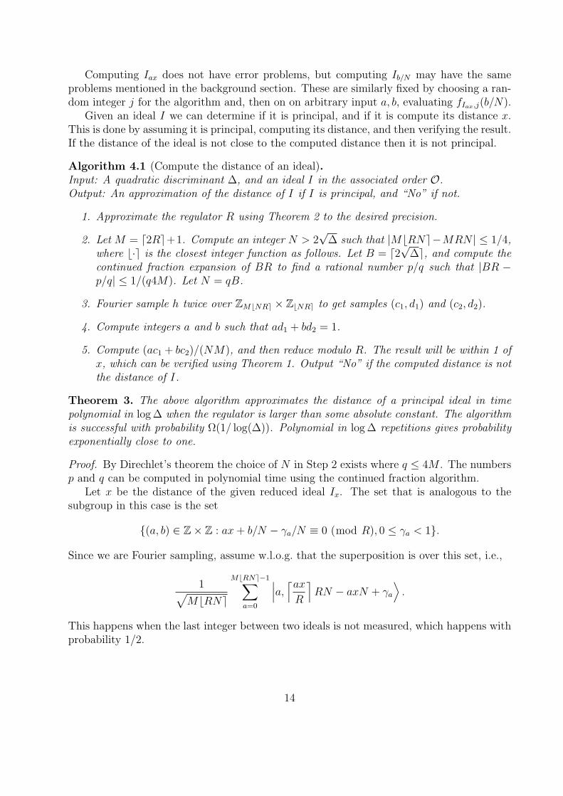
Algorithm 4.1 (Compute the distance of an ideal).Input: A quadratic discriminant ∆, and an ideal I in the associated order O.Output: An approximation of the distance of I if I is principal, and “No” if not.

1. Approximate the regulator R using Theorem 2 to the desired precision.

2. Let M = d2Re+1. Compute an integer N > 2√

∆ such that |MbRNe−MRN | ≤ 1/4,where b·e is the closest integer function as follows. Let B = d2

√∆e, and compute the

continued fraction expansion of BR to find a rational number p/q such that |BR −p/q| ≤ 1/(q4M). Let N = qB.

3. Fourier sample h twice over ZMbNRe × ZbNRe to get samples (c1, d1) and (c2, d2).

4. Compute integers a and b such that ad1 + bd2 = 1.

5. Compute (ac1 + bc2)/(NM), and then reduce modulo R. The result will be within 1 ofx, which can be verified using Theorem 1. Output “No” if the computed distance is notthe distance of I.

Theorem 3. The above algorithm approximates the distance of a principal ideal in timepolynomial in log ∆ when the regulator is larger than some absolute constant. The algorithmis successful with probability Ω(1/ log(∆)). Polynomial in log ∆ repetitions gives probabilityexponentially close to one.

Proof. By Direchlet’s theorem the choice of N in Step 2 exists where q ≤ 4M . The numbersp and q can be computed in polynomial time using the continued fraction algorithm.

Let x be the distance of the given reduced ideal Ix. The set that is analogous to thesubgroup in this case is the set

(a, b) ∈ Z× Z : ax + b/N − γa/N ≡ 0 (mod R), 0 ≤ γa < 1.

Since we are Fourier sampling, assume w.l.o.g. that the superposition is over this set, i.e.,

1√MbRNe

MbRNe−1∑a=0

∣∣∣a,⌈ax

R

⌉RN − axN + γa

⟩.

This happens when the last integer between two ideals is not measured, which happens withprobability 1/2.

14

We will show that with large probability, a sample (c, d) is such that cNM

− γd

NM≡

dx mod R, where −1/2 ≤ γd ≤ 1/2. Rewriting this condition, let c = dxNM −bdxRcRNM +

γd. The Fourier transform at |c, d〉 is

1

MbRNe√bRNe

MbRNe−1∑a=0

ωac+bdMMbRNe .

Writing out ac + bdM we get

adxNM − a

⌊dx

R

⌋RNM + aγd + d

⌈ax

R

⌉RNM − adxNM + dMγa

=

(d⌈ax

R

⌉− a

⌊dx

R

⌋)RNM + aγd + dMγa.

Let λ = bRNe. Reducing modulo M bRNe = M(RN + λ) gives −λM(d⌈

axR

⌉− abdx

Rc) +

aγd + dMγa. Rewriting⌈

axR

⌉as ax

R+ δa and bdx

Rc as dx

R− δd, with 0 ≤ δa, δd < 1, we get

a(γd + λMδd) + dM(γa − λδa).By choice of N and M , λ ≤ 1/(4M), so a|γd + λMδd|/(MbRNe) ≤ |γd + λMδd| ≤ 3/4.

When d ≤ bRNe/ log(MbRNe) it follows that dM(γa − λδa)/(MbRNe) ≤ 1/ log(MbRNe).By Claim 3.1 the probability of seeing such a sample d ≤ bRNe/ log(MbRNe) is at leastΩ(1/bRNe).

There are bRNe values d so if d ≤ bRNe/ log(MbRNe) then d is measured with prob-ability Ω(1/ log(MbRNe)). The probability of measuring two relatively prime values usingthis procedure is at least Ω(ε2/ log(MbRNe)4), where ε = 1/2. Since MRN is polynomialin ∆, this is with probability at least Ω(1/(log ∆)4).

For the classical reconstruction, suppose we start with such a pair. Then

c1 = d1xNM −⌊

d1x

R

⌋RNM + γd1 ,

c2 = d2xNM −⌊

d2x

R

⌋RNM + γd2 ,

and

ac1 + bc2 = xNM −(

a

⌊d1x

R

⌋+ b

⌊d2x

R

⌋)RNM + aγd1 + bγd2 .

After dividing by NM we have,

x−(

a

⌊d1x

R

⌋+ b

⌊d2x

R

⌋)R + (aγd1 + bγd2)/(NM).

Since a and b are at most the maximum of d1 and d2,

(aγd1 + bγd2)/(NM) ≤ 2bRNe/(NM) ≤ 1

by our choice of M . Therefore reducing modulo R, where R has high enough precision, willresult in x ± 1, which can be verified and recomputed to a better accuracy using classicalalgorithms.

15

5 Class Group Computations

In this section we show how to compute the class group G and class number of a real quadraticnumber field. The class group G is a finite abelian group and given a set of generators, thetask is to decompose it as G = ×Zei

such that ei|ei+1. In its simplest form, when there is aunique bit string representing each element in the group, decomposing a finite abelian groupreduces to a hidden subgroup problem. The problem we must deal with here is that it isnot known how to efficiently compute a unique representative for an element in the classgroup. After reviewing how the unique representation case reduces to the hidden subgroupproblem, we will show how to use then algorithm from Section 4 to create a superpositionover an arbitrary equivalence class, allowing the HSP algorithm to carry through.

Decomposing a finite abelian group given a set of generators g1, . . . , gk reduces to a hiddensubgroup problem over Zk as follows. The HSP instance is the function f(e1, . . . , ek) =∑k

i=1 eigi. The hidden subgroup is the lattice of relations L ⊆ Zk where [e1, . . . , ek] ∈ L iff∑i eigi = 0. The hidden subgroup problem algorithm can be used to find a basis matrix

B whose columns span L. The Smith normal form of B then reveals the group structure.In particular, in (classical) polynomial-time, unimodular matrices U, V are computed suchthat UBV = D, where D is a diagonal matrix. The elements on the diagonal of D are[e1, e2, . . . , ek, 1, . . . , 1] where ei|ei+1, which are the orders of the cyclic factors of G ∼= ×iZei

,and [g′1, . . . , g

′n] = [g1, . . . , gn]U−1 gives a basis for the group.

Recall the definitions of I and P from Section 2.2. I is the set of invertible ideals and isa group under multiplication (·). P is the set of principal invertible ideals, and is a subgroupof I. The class group is defined as the quotient group Cl = I/P . The set of reduced ideals Ris a finite subset of I. Any ideal I ∈ I and the ideal resulting after reduction are in the sameequivalence class modulo P . Therefore, the class group is finite since R is. Just as there isa cycle of reduced principal ideals, there is a cycle of reduced ideals for each group element.This cycle can have exponential size, and is different for each element in the class group inthat it can have a different number of reduced ideals and a different set of distances betweenall the ideals in the class. In addition, only a relative distance is defined between two ideals(given two equivalent ideals I and J , defined as the distance of I−1J), so in general there isno ideal to single out with distance zero.

It is not known how to test identity efficiently in the class group classically. An efficientquantum identity test does follow from our principal ideal test, since given two ideals Iand J , it can be tested if I−1J is principal. Assuming the GRH, it is possible to computea polynomial size set of generators for the class group in polynomial time [Coh93]. Thebest classical algorithms for computing the regulator compute the class group at the sametime [Buc89]. The standard quantum algorithm for decomposing a group cannot be directlyapplied since we do not have unique representatives for each group element. After multiplyingtwo elements, we are left with a reduced ideal, but it could be any reduced ideal in the cycle.

Here we deal with the fact that we cannot define an HSP instance as above since eachgroup element has a potentially exponential number of representatives (i.e. reduced ideals).The natural approach is to replace a basis state |g〉 with a superposition of elements in theequivalence class, preserving the property that two different class group elements are mappedto orthogonal vectors. Such an approach has been used before, such as in [Wat01]. Here we

16

have the added difficulty that we are computing on the set of reduced ideals, which is not agroup, and that each equivalence class has a different number of such ideals.

To use the standard HSP algorithm to decompose the group we will now show how tocompute a quantum state |φe1,...,ek

〉 given a set of coefficients e1, . . . , ek for the group element∑i eigi. These states must satisfy two properties for the HSP algorithm to work. First, the

states must have exponentially small inner product when the group elements are different.Second, if the same group element is computed from two different coefficient vectors, thenthe resulting states must have inner product exponentially close to one. Roughly speaking,this will be achieved by creating a superposition of all reduced ideals in the class. Ideals indifferent classes are different, so orthogonality is achieved. Some more care must be takenwhen ideals are in the same class and states will only be exponentially close.

Recall Definition 2.1 and suppose for a given reduced ideal I, fI(i/N) = (J, δ). LetN ∈ Z. Then define fI,N : Z → I × Z by fI,N(i) = (J, k), where k = bNδc. Define the state

|φe1,...,ek〉 = |φI〉 = 1√

bNRe

∑bNRe−1i=0 |fI,N(i)〉, where I =

∑eigi.

Claim 5.1. If I and J are the same element of the class group, then |φI〉 and |φJ〉 haveinner product at least 1−

√∆/N .

Proof. Consider a segment between ideal J and the next ideal J ′. There are at least N/√

∆rational numbers mapped into this region. As in the analysis in Lemma 3.2 this numberis always M or M + 1 for some M depending J . Therefore the two vectors have commonsupport of at least a 1−

√∆/N fraction of basis vectors.

The rounding problem mentioned in the introduction can be fixed by using the functionsfJ,j. The choice of L must be taken larger by an exponential factor than the total numberof reduced ideals, which is at most ∆ [Len82b]. For simplicity we list fJ below.

Algorithm 5.1 (Group element to quantum state map).Input: A set of coefficients e1, . . . , ek.Output: An approximation of the quantum state |φe1,...,ek

〉 = 1√bNRe

∑bNRe−1i=0 |fI(i)〉, where

I =∑

eigi.

1. Approximate the regulator R using Algorithm 3.1. Let N = ∆.

2. Compute the ideal I =∑

i eigi, resulting in |I〉.

3. Split into a superposition of distances and evaluate fI to get∑bNRc−1

i=0 |I, i, fI(i)〉.

4. Use Algorithm 4.1 to compute i/N with exponentially high probability.

5. Erase the second register, which contains i.

6. Uncompute i/N , resulting in a state exponentially close to 1√bNRe

∑bNRe−1i=0 |I, fI(i)〉.

7. Uncompute I from e1, . . . , ek, resulting in 1√bNRe

∑bNRe−1i=0 |fI(i)〉.

17

Using this algorithm in the standard hidden subgroup problem algorithm for the functionevaluation shows:

Corollary 5.1. The class group and class number of a real quadratic number field can befound in quantum polynomial-time assuming the GRH.

6 Open Problems

In this paper we solved some problems from computational algebraic number theory. Givenan order O of a real quadratic number field Q(

√d) we showed how to compute the regulator,

how to compute the distance of an ideal, and how to compute the class group. For higherdimensional number fields, there are a number of problems still open. In this paper we lookedat quadratic number fields, which means that K has degree two over Q. To get a numberfield of degree n a root of a degree n equation is adjoined to Q. The open problems includefinding the class group and class number, the group of units and regulator, and solving theprincipal ideal problem. This list can be found in [Coh93, pg. 217].

We should also point out that there are similar questions for imaginary quadratic numberfields, which are defined similarly with d being negative. The problems here are much easierhowever. Finding units is now polynomial time and there are only a finite number. Factoringreduces to computing the class group, but quantum algorithms for computing the class groupare automatic from standard quantum techniques, because each group element has a uniqueefficiently computable representative.

Finally we mention that the following problems for quadratic number fields are in NP ∩co−NP assuming the GRH [BW91] and assuming a constant degree number field: decidingif an ideal is principal, deciding if a set of ideals generate the class group, deciding if a setof ideals are a basis for the class group.Acknowledgments: Thanks to Hendrik Lenstra for many useful discussions and for sug-gesting these problems. Also thanks to Kirsten Eisentrager, Richard Jozsa, Ashwin Nayak,Umesh Vazirani, and Ulrich Vollmer for useful discussions.

References

[BTW95] Johannes Buchmann, Christoph Thiel, and Hugh C. Williams. Short representa-tion of quadratic integers. In Wieb Bosma and Alf J. van der Poorten, editors,Computational Algebra and Number Theory, Sydney 1992, volume 325 of Mathe-matics and its Applications, pages 159–185. Kluwer Academic Publishers, 1995.

[Buc89] J. Buchmann. A subexponential algorithm for the determination of class groupsand regulators of algebraic number fields. In Seminaire de theorie des nombres,pages 28–41. Paris, 1989.

[BV97] Ethan Bernstein and Umesh Vazirani. Quantum complexity theory. SIAM Journalon Computing, 26(5):1411–1473, October 1997.

18

[BW89a] Johannes Buchmann and H. C. Williams. On the existence of a short proof forthe value of the class number and regulator of a real quadratic field. In Numbertheory and applications (Banff, AB, 1988), pages 327–345. Kluwer Acad. Publ.,Dordrecht, 1989.

[BW89b] Johannes A. Buchmann and Hugh C. Williams. A key exchange system basedon real quadratic fields (extended abstract). In G. Brassard, editor, Advancesin Cryptology—CRYPTO ’89, volume 435 of Lecture Notes in Computer Science,pages 335–343. Springer-Verlag, 1990, 20–24 August 1989.

[BW91] Johannes Buchmann and Hugh C. Williams. Some remarks concerning the com-plexity of computing class groups of quadratic fields. Journal of Complexity,7(3):311–315, 1991.

[Coh93] Henri Cohen. A course in computational algebraic number theory, volume 138 ofGraduate Texts in Mathematics. Springer-Verlag, 1993.

[EHK99] Mark Ettinger, Peter Høyer, and Emanuel Knill. Hidden subgroup states arealmost orthogonal. Technical report, quant-ph/9901034, 1999.

[FIM+03] Katalin Friedl, Gabor Ivanyos, Frederic Magniez, Miklos Santha, and Pranab Sen.Hidden translation and orbit coset in quantum computing. In Proceedings of theThirty-Fifth Annual ACM Symposium on Theory of Computing, San Diego, CA,9–11 June 2003.

[GSVV01] Michaelangelo Grigni, Leonard Schulman, Monica Vazirani, and Umesh Vazirani.Quantum mechanical algorithms for the nonabelian hidden subgroup problem. InProceedings of the Thirty-Third Annual ACM Symposium on Theory of Computing,Crete, Greece, 6–8 July 2001.

[Hal02] Sean Hallgren. Polynomial-time quantum algorithms for Pell’s equation and theprincipal ideal problem. In Proceedings of the Thirty-Fourth Annual ACM Sympo-sium on Theory of Computing, pages 653–658, Montreal, Quebec, Canada, 19–21May 2002.

[HRTS00] Sean Hallgren, Alexander Russell, and Amnon Ta-Shma. Normal subgroup recon-struction and quantum computation using group representations. In Proceedingsof the Thirty-Second Annual ACM Symposium on Theory of Computing, pages627–635, Portland, Oregon, 21–23 May 2000.

[IMS01] Gabor Ivanyos, Frederic Magniez, and Miklos Santha. Efficient quantum algorithmsfor some instances of the non-abelian hidden subgroup problem. In Proceedings ofthe Thirteenth Annual ACM Symposium on Parallel Algorithms and Architectures,pages 263–270, Heraklion, Crete Island, Greece, 4-6 July 2001.

[Joz03] Richard Jozsa. Notes on Hallgren’s efficient quantum algorithm for solving Pell’sequation. Technical report, quant-ph/0302134, 2003.

19

[Kup03] Greg Kuperberg. A subexponential-time quantum algorithm for the dihedral hid-den subgroup problem. Technical report, quant-ph/0302134, 2003.

[Len82a] Hendrik W. Lenstra, Jr. On the calculation of regulators and class numbers ofquadratic fields. In J. V. Armitage, editor, Journees Arithmetiques, Exeter 1980,volume 56 of London Mathematical Society Lecture Notes Series, pages 123–150.Cambridge University Press, 1982.

[Len82b] H. W. Lenstra, Jr. On the computation of regulators and class numbers of quadraticfields. Lond. Math. Soc. Lect. Note Ser., 56:123–150, 1982.

[Len02] H. W. Lenstra, Jr. Solving the Pell equation. Notices Amer. Math. Soc., 49(2):182–192, February 2002.

[LL93] A.K. Lenstra and H.W. Lenstra, editors. The Development of the Number FieldSieve, volume 1544 of Lecture Notes in Mathematics. Springer–Verlag, 1993.

[MRRS04] Cris Moore, Daniel Rockmore, Alexander Russell, and Leonard Schulman. Thehidden subgroup problem in affine groups: Basis selection in fourier sampling.In Proceedings of the Fifteenth Annual ACM-SIAM Symposium on Discrete Algo-rithms, New Orleans, LA, 11–13 January 2004.

[NZM91] Ivan Niven, Herbert S. Zuckerman, and Hugh L. Montgomery. An introduction tothe theory of numbers. John Wiley & Sons Inc., New York, fifth edition, 1991.

[Sch86] A. Schrijver. Theory of Linear and Integer Programming, chapter 15.1 : Kar-markar’s polynomial–time algorithm for linear programming, pages 190–194. JohnWiley&Sons, New York, 1986.

[Sho97] Peter W. Shor. Polynomial-time algorithms for prime factorization and discretelogarithms on a quantum computer. SIAM Journal on Computing, 26(5):1484–1509, October 1997.

[Sho03] Peter W. Shor. Why haven’t more quantum algorithms been found? Journal ofthe ACM, 50(1):87–90, January 2003.

[Sim97] Daniel R. Simon. On the power of quantum computation. SIAM Journal onComputing, 26(5):1474–1483, October 1997.

[vDHI03] Wim van Dam, Sean Hallgren, and Lawrence Ip. Quantum algorithms for somehidden shift problems. In Proceedings of the Fourteenth Annual ACM-SIAM Sym-posium on Discrete Algorithms (SODA), Baltimore, MD, 2003.

[Vol00] Ulrich Vollmer. Asymptotically fast discrete logarithms in quadratic number fields.In Algorithmic Number Theory Symposium IV, volume 1838, pages 581–594, 2000.

[Wat01] John Watrous. Quantum algorithms for solvable groups. In Proceedings of theThirty-Third Annual ACM Symposium on Theory of Computing, pages 60–67,Crete, Greece, 6–8 July 2001.

20

[Wil00] H. C. Williams. Solving the pell equation. In Proc. Millennial Conference onNumber Theory, volume 3, pages 397–435, 2000.

21