Embed Size (px)
Citation preview

QU-CHEE-PRG-TR--2017-25
PRG 025 ©January 2017
QUEEN'S UNIVERSITY
POLYMERS RESEARCH GROUP
19 Division Street, Kingston, ON, K7L 3N6 Canada
EXACT ANALYTICAL SOLUTION FOR LARGE-AMPLITUDE OSCILLATORY SHEAR FLOW
FROM OLDROYD 8-CONSTANT FRAMEWORK: SHEAR STRESS
C. Saengow1,3,4, A.J. Giacomin1,2,* and C. Kolitawong3
1Polymers Research GroupChemical Engineering Department
2Mechanical and Materials Engineering Department Queen’s University
Kingston, Ontario, CANADA K7L 3N6
3Mechanical and Aerospace Engineering Department Polymer Research Center
King Mongkut’s University of Technology North Bangkok Bangkok, THAILAND 10800
4College of Integrated Science and Technology Rajamangala University of Technology Lanna
Doisaket, Chiangmai, THAILAND 50220
This report is circulated to persons believed to have an active interest in the subject matter; it is intended to furnish rapid communication and to stimulate comment, including corrections of
possible errors.
*Corresponding author ([email protected])

EXACT ANALYTICAL SOLUTION FOR LARGE-AMPLITUDE OSCILLATORY SHEAR FLOW
FROM OLDROYD 8-CONSTANT FRAMEWORK: SHEAR STRESS
C. Saengow1,3,4, A.J. Giacomin1,2,* and C. Kolitawong3
1Polymers Research GroupChemical Engineering Department
2Mechanical and Materials Engineering Department Queen’s University
Kingston, Ontario, CANADA K7L 3N6
3Mechanical and Aerospace Engineering Department Polymer Research Center
King Mongkut’s University of Technology North Bangkok Bangkok, THAILAND 10800
4College of Integrated Science and Technology Rajamangala University of Technology Lanna
Doisaket, Chiangmai, THAILAND 50220
ABSTRACT
The Oldroyd 8-constant model is a continuum framework containing, as special cases, many important constitutive equations for elastic liquids. When polymeric liquids undergo large-amplitude oscillatory shear flow, the shear stress responds as a Fourier series, the higher harmonics of which are caused by the fluid nonlinearity. We choose this framework for its rich diversity of special cases (we tabulate 14 of these). Deepening our understanding of this Oldroyd 8-constant framework thus at once deepens our understanding of every one of these special cases. Previously [Macromol Theor Simul, 24, 352 (2015)], we arrived at an exact analytical solution for the corotational Maxwell model. Here, we derive the exact analytical expression for the Oldroyd 8-constant framework for the shear stress response in large-amplitude oscillatory shear flow. Our exact solution reduces to our previous solution for the special case of the corotational Maxwell model, as it should. Our worked example uses the special case of the corotational Jeffreys model to explore the role of on the higher harmonics. Keywords: Large-amplitude oscillatory shear; LAOS; Oldroyd 8-constant model; higher harmonics.
*Corresponding author ([email protected])
η∞

2
CONTENTS I. INTRODUCTION ................................................................................................... 5
a. Oscillatory Shear Flow ....................................................................................... 6 b. Oldroyd 8-Constant Framework ...................................................................... 7
i. Steady Shear .................................................................................................................. 9 ii. Small-Amplitude Oscillatory Shear (SAOS) ............................................................. 10
II. METHOD ............................................................................................................... 10 a. Transient Parts of the Stress Responses ........................................................ 11 b. Particular Part of the Stress Responses ......................................................... 13
III. RESULTS: SHEAR STRESS ................................................................................. 13 a. Exact Solution .................................................................................................... 13 b.
⌣τ zz and ⌣τ zz 0( ) Invariance ................................................................................ 16
IV. CONSISTENCY CHECKS .................................................................................... 17 a. SAOS ................................................................................................................... 17 b. Steady Shear Flow ............................................................................................ 18 c. LAOS .................................................................................................................. 18
i. Goddard Integral Approximation ................................................................................ 19 ii. Finite Difference Solution .......................................................................................... 21
V. WORKED EXAMPLE: η∞ AND THE HIGHER HARMONICS .................... 21
VI. CONCLUSION ...................................................................................................... 22 VII. ACKNOWLEDGMENT .................................................................................. 23 VIII. APPENDICES ................................................................................................... 23
a. Deriving Four Differential Equations in S , N1 , N2 and ⌣τ zz ...................... 23
b. Solving Eqs. (46)–(49) by the Kovacic Method ............................................. 26 c. Evaluating
limWi→0
of Eq. (60) for SAOS ............................................................. 27
IX. REFERENCES ........................................................................................................ 50

3
TABLES
Table I: Literature on Analytical Solutions for Large-Amplitude Oscillatory
Shear Flow....................................................................................................................................31Table II: Dimensional Variables.................................................................................................33Table III: Dimensionless Variables and Groups................................................................35Table IV: Models Included in the Oldroyd 8-Constant Framework (see TABLE
8.1-1 of [21] and TABLE 7.3-2 of [29])............................................................................37
FIGURES
Figure 1: Liquid motion (Cartesian coordinates) in sliding-plate rheometer with oscillating upper plate. Particle trajectories, red for 0 <ωt < π 2 , blue for π <ωt < 3π 2 [Eq. (1)]. Newtonian velocity profile is
vx V0 = y h( )cosωt . ............................................................................................. 38 Figure 2: Diagram for LAOS illustrating the complex, dimensionless
generalized non-Newtonianness, Gn . Newtonian behavior is observed well inside the red unit circle, where Gn ≪1 . The magnitude of Gn thus reflects how far the system departs from Newtonian behavior and the inclination
⌢φ identifies the type of departure. ................................................ 39
Figure 3: Dimensionless shear stress versus Weissenberg number with curves of constant σ = 1
100 , 19 , 1
4 ,1 from bottom to top [Eq. (29)]. Blue curve (second from the bottom) shows the critical value of σ = 1 9 for shear-stress monotonicity [Eq. (31)]. ...................................................................................... 40
Figure 4: Illustration of consistency between SAOS predictions of Eq. (60) (red) [ λ2 = µ0 = µ1 = µ2 = ν1 = ν2 = 0 ] and Eq. (36) (black) [ λ2 λ1 = 0 ]. Both use
Wi = 1100 , De = 1 . .................................................................................................. 41
Figure 5: Illustration of consistency between our new exact solution for Oldroyd 8-constant framework (black) [Eq. (60) with λ2 = µ0 = µ1 = µ2 =
ν1 = ν2 = 0 ] and the one from corotational Maxwell model (red) (Eq. (81); see also Figure 18 of [9]) for steady shear flow at very low Deborah number [ Wi = 1
2 , De = 1100 ]. ................................................................................. 42
Figure 6: Comparison of analytical exact solution [Eq. (74) (black)] and our previous work [Eq. (66) of [9] (red)] for loops of minus dimensionless shear stress, versus dimensionless shear rate for Wi De = 1
10 , 12 , 3
4 ,1, 54 for each De .
4
Special case of the corotational Maxwell fluid ( η∞ η0 =λ2 λ1 = 0 , µ0 = µ1 =
µ2 = ν1 = ν2 = 0 ). ................................................................................................... 43 Figure 7: Comparison of analytical exact solution [Eq. (82) in black] and
Goddard integral expansion solution [Eq. (86) in red] for loops of minus dimensionless shear stress, versus dimensionless shear rate for
Wi De = 110 , 1
2 , 34 ,1, 5
4 for each De . Special case of the corotational Jeffreys fluid ( η∞ η0 =λ2 λ1 = 1 27 , µ0 = µ1 = µ2 = ν1 = ν2 = 0 ). .................................. 44
Figure 8: Comparison of analytical exact solution [Eq. (82) in black] and Goddard integral expansion solution [Eq. (86) in red] for loops of minus dimensionless shear stress, versus dimensionless shear rate for
Wi De = 110 , 1
2 , 34 ,1, 5
4 for each De . Special case of the corotational Jeffreys fluid ( η∞ η0 =λ2 λ1 = 1 9 , µ0 = µ1 = µ2 = ν1 = ν2 = 0 ). .................................... 45
Figure 9: Comparison of analytical exact solution [Eq. (82) in black] and Goddard integral expansion solution [Eq. (86) in red] for loops of minus dimensionless shear stress, versus dimensionless shear rate for
Wi De = 110 , 1
2 , 34 ,1, 5
4 for each De . Special case of the corotational Jeffreys fluid ( η∞ η0 =λ2 λ1 = 1 3 , µ0 = µ1 = µ2 = ν1 = ν2 = 0 ). .................................... 46
Figure 10: Comparison of analytical exact solution [Eq. (82) in black] and finite difference solution (red) for shear stress [solving Eqs. (41)–(43) with Eq. (87)] for loops of minus dimensionless shear stress, versus dimensionless shear rate for Wi De = 1
10 , 12 , 3
4 ,1, 54 for each De . Special case of the
corotational Jeffreys fluid ( λ2 λ1 = 1 3 , µ0 = µ1 = µ2 = ν1 = ν2 = 0 ). ............. 47 Figure 11: Comparison of analytical exact solution [Eq. (82) in black] and finite
difference solution (red) for shear stress [solving Eqs. (41)–(43) with Eq. (87)] for loops of minus dimensionless shear stress, versus dimensionless shear rate for Wi De = 1
10 , 12 , 3
4 ,1, 54 for each De . Special case of the
corotational Jeffreys fluid ( λ2 λ1 = 1 9 , µ0 = µ1 = µ2 = ν1 = ν2 = 0 ).. ............ 48 Figure 12: Comparison of analytical exact solution [Eq. (82) in black] and finite
difference solution (red) for shear stress [solving Eqs. (41)–(43) with Eq. (87)] for loops of minus dimensionless shear stress, versus dimensionless shear rate for Wi De = 1
10 , 12 , 3
4 ,1, 54 for each De . Special case of the
corotational Jeffreys fluid ( λ2 λ1 = 1 27 , µ0 = µ1 = µ2 = ν1 = ν2 = 0 ). ........... 49

5
I. INTRODUCTION Large-amplitude oscillatory shear (LAOS) flow experiments have been used
to investigate the physics of complex liquids (see [1]; Ch. 11 of [2]). Since its conception in 1935 [3,4,5] oscillatory shear flow has become by far the most popular laboratory method for exploring the physics of polymeric liquids. We generate oscillatory shear flow by confining the fluid to a simple shear apparatus, and then subject one solid-liquid boundary to a coplanar sinusoidal displacement (see Figure 1) generating a corresponding cosinusoidal shear rate:
!γ t( ) = !γ 0 cosωt (1) Using the characteristic relaxation time of the viscoelastic fluid, λ1 , we can nondimensionalize Eq. (1):
λ1 !γ t( ) = WicosDe t/λ1( ) (2) where:
De ≡ λ1ω (3) and:
Wi ≡ λ1 !γ0 (4)
are the Deborah and Weissenberg numbers. In this paper, we define dimensional symbols in Table II, and dimensionless ones in Table III (which follow Tables 2 and 3 of [6] with adaptations for [7]).
Increasing either the Weissenberg number or the Deborah number in Eq. (2) can cause the fluid response to depart from Newtonian behavior. We can construct a complex dimensionless number from the ordered pair De,Wi( ) thus (see Figure 2 or Fig. 1. of [6]): Gn ≡ De+ i Wi (5) which defines a vector with magnitude:
Gn ≡ De2+ Wi2 (6) and with angle:
⌢φ ≡ arctan Wi De( ) (7) We can associate behavior in steady shear flow with De = 0 , where Gn = i Wi . We further associate linear viscoelastic behavior with Wi = 0 , where Gn = De . The Gn thus reflects how far the fluid behavior departs from Newtonian
behavior. The value ⌢φ = 0 corresponds to linear viscoelastic behavior, and
⌢φ = π 2 , to steady shear flow. The angle
⌢φ thus reflects the type of departure
from Newtonian behavior. When higher harmonics are observed in the shear stress response, we call
the oscillatory experiment large-amplitude. By higher harmonics, we mean contributions to the shear stress at odd multiples of the test frequency:

6
τ yx τ , !γ 0( )!γ 0 = − ′′ηn ω , !γ 0( )cosnτ + ′ηn ω , !γ 0( )sinnτ
n=1,2
∞
∑ (8)
For polymeric liquids, these higher harmonics are commonly observed when:
Wi De > 1 (9) and when:
Gn > 1 (10) Eqs. (9) or (10) are thus our working definition of large-amplitude oscillatory shear flow [1,8,9], and with recent advances in rheometry, conducting experiments satisfying Eqs. (9) or (10) are now commonplace for exploring the physics of complex liquids [10]. Eqs. (9) or (10) are refinement on the previous definition of large-amplitude (see Eq. (8) of [6]). Many notations have been introduced for analyzing the higher harmonics in the shear stress (see Section 9 of [6]) or in the normal stress differences (see Section 10 of [6]). In this paper, we follow Dealy et al. (1973) in plotting loops of shear stress versus shear rate, since these best bring out material nonlinearities as distortions from ellipticity [11,12,13].
Table I classifies (chronologically according to first findings) the constitutive equations that have lead to analytical solutions to the stress responses in large-amplitude oscillatory shear flow. From second column from the last, we learn that we have just one exact solution for large-amplitude oscillatory shear flow, and this, for the corotational Maxwell model [9]. With some difficulty, this solution was arrived at using the method of Kovacic [14] and variation of variable [15]. From Table I, we glean that the literature contains one and only one exact solution for the shear stress response of a complex fluid in LAOS (see third row from the bottom of Table I). A method has also been proposed for arrive at approximate analytical solutions to K-BKZ integral models in LAOS (see Appendix B of [16] or Subsection 2.2.5 of Chapter 11 of [2]).
In this paper, we undertake the more ambitious project of arriving at analytical solution for large-amplitude oscillatory shear flow for an entire framework of constitutive equations. Specifically, we choose the Oldroyd 8-constant framework. We choose this framework for its rich diversity of important special cases which we will discuss in the Subhead of Subsection I.b.
a. Oscillatory Shear Flow
In the absence of fluid inertia [17], for isothermal [17,18,19] oscillatory simple shear flow, the rate of deformation tensor is given by:
!γ =0 !γ 0!γ 0 00 0 0
⎡
⎣
⎢⎢⎢
⎤
⎦
⎥⎥⎥≡
0 !γ 0 cosωt 0
!γ 0 cosωt 0 00 0 0
⎡
⎣
⎢⎢⎢⎢
⎤
⎦
⎥⎥⎥⎥
(11)

7
and for any simple shear flow (see Eq. (19) of [20]):
12
ω ⋅ τ − τ ⋅ω{ } = 12
−2τ yx τ xx −τ yy 0τ xx −τ yy 2τ yx 0
0 0 0
⎡
⎣
⎢⎢⎢⎢
⎤
⎦
⎥⎥⎥⎥
!γ (12)
and:
12
ω ⋅ !γ − !γ ⋅ω{ } =−1 0 00 1 00 0 0
⎡
⎣
⎢⎢⎢
⎤
⎦
⎥⎥⎥!γ 2 (13)
which we will use in Subsection VIII.a below.
b. Oldroyd 8-Constant Framework The Oldroyd 8-constant framework is given by (see Eq. (8.1-2) in [21]; [22]):
τ + λ1D τD t
+ 12 µ0 trτ( ) !γ − 1
2 µ1 τ ⋅ !γ + !γ ⋅ τ{ }+ 12ν1 τ : !γ( )δ−−−−−−−−−−−−−
= −η0!γ + λ2
D !γD t
− µ2 !γ ⋅ !γ{ }+ 12ν2 !γ : !γ( )δ
−−−−−−−−−−−−−−
⎛⎝⎜
⎞⎠⎟
(14)
Eq. (14) reduces exactly to a rich diversity of special cases. We tabulate 14 of these in Table IV, first in descending order of the number of material constants (column 2), and next according to relevance (column 3). By relevance, we mean the number of shear stress harmonics predicted. From columns 2 and 3, we find the corotational Maxwell to be the simplest relevant special case of the Oldroyd 8-constant framework. Deepening our understanding of the Oldroyd 8-constant framework thus deepens our understanding of every one of the important special cases in Table IV. Moreover, an exact solution for the Oldroyd 8-constant framework would thus, of course, provide an exact solution for each of the important special cases in Table IV.
The Oldroyd 8-constant framework has also been closely connected, albeit approximately, with macromolecular theory ([23,24,25]; see Table 1 of [26]; see Eqs. (32) of [27],[28]; see Tables 6.2-1 and 6.2-2 of [29]; Problems 11B.9 and 11B.10 of [30]; §IV and §V. of [31]; §9.5 of [21]). For instance, for rigid dumbbells suspended in a Newtonian solvent:
ηp = nkTλ , λ1 = λ , λ2 = 2λ 5 , µ0 = −2λ 7 ,µ1 = −λ 7 , µ2 = −26λ 35 , ν1 = ν2 = 0
(15)
where λ is the characteristic time (Table 1 of [26]). With Eqs. (15), the Oldroyd 8-constant framework thus provides a useful approximation to the polymer contribution to the stresses for a suspension of rigid dumbbells [26]. Further, for finitely extensible nonlinear elastic (FENE) dumbbells:

8
ηp =bnkTλH
b+ 5, λ1 =
b 2b+11( )λH
2b+ 7( ) b+ 9( ) , λ2 =−14bλH
2b+ 7( ) b+ 7( ) b+ 9( ) ,
µ0 =−6bλH
2b+ 7( ) b+ 5( ) b+ 9( ) , µ1 =b 2b+ 3( )λH
2b+ 7( ) b+ 9( ) , µ2 =−2b 4b+ 21( )λH
2b+ 7( ) b+ 7( ) b+ 9( ) ,
ν1 = ν2 = 0
(16)
where λH is the characteristic time (Table 1 of [26]). With Eqs. (16), the Oldroyd 8-constant framework thus provides a useful approximation to the polymer contribution to the stresses for FENE dumbbells [26].
The corotational Jeffreys model µ0 = µ1 = µ2 = ν1 = ν2 = 0( ) is classified in row seven of Table IV, and we will use this special case below as a worked example to demonstrate the usefulness of our results (see Section V). The dashed-underlined terms in Eq. (14) represent higher order nonlinear contributions. In Eq. (14), the total stress tensor is given by:
π ≡ τ + pδ (17) and the rate-of-deformation tensor:
!γ ≡ ∇v + ∇v( )† (18) and the vorticity tensor is defined by:
ω ≡ ∇v − ∇v( )† (19) The corotational derivative for stress tensor is given by:
D τ
D t≡
Dτ
Dt+ 1
2 ω ⋅ τ − τ ⋅ ω{ } (20)
and, for shear rate tensor, by:
D !γ
D t≡
D !γDt
+ 12 ω ⋅ !γ − !γ ⋅ ω{ } (21)
In Eq. (17), δ is the kronecker delta. The Oldroyd 8-constant model can be remarkably useful in polymer processing when it leads to analytical solutions, as it does for wire coating (Case III in [32]), and to a corrugated wire coated through a corrugated die (see Section 3. of [33]; Section 2. of [34]), and in plastic pipe extrusion for elliptical pipe ([35,36]), and also to extrusion from an eccentric annular pipe die (Case II in [32],[37],[38;39]).
Eq. (14) can be written in integral form (see EXAMPLE 8.1-2 of [21]), or rewritten in terms of the upper convected derivative (see Eq. 7.3-2 of [30]). The footnote on page 354 of [30] relates the parameters of Eq. 7.3-2 of [30] to those of our Eq. (14).
We close this subhead by noting that Eq. (14) has also been approximately connected to the Rivlin-Ericksen, Spriggs 6-constant and Giesekus fluids (see Appendix of [40]).

9
i. Steady Shear
For steady shear flow, the viscometric functions for the Oldroyd 8-constant framework are given by (see Eqs. (12)–(14) of [22]; Eqs. (14), (22) and (23) of [41]):
η !γ( )η0
= −Ψ1 !γ( )Ψ10
λ2
λ1−1⎛
⎝⎜⎞⎠⎟+λ2
λ1=Ψ2 !γ( )Ψ20
λ1 − λ2 − µ1 + µ2
λ1 − µ1
⎛⎝⎜
⎞⎠⎟+λ2 − µ2
λ1 − µ1=
1+σ 2 !γ2
1+σ 1 !γ2 (22)
where:
Ψ10 ≡ lim
!γ →0Ψ1 = 2η0 λ1 − λ2( ) (23)
Ψ20 ≡ lim
!γ →0Ψ2 = −η0 λ1 − λ2 − µ1 + µ2( ) (24)
and where:
σ 1 ≡ λ12 + µ0 µ1 − 3
2ν1( )− µ1 µ1 −ν1( ) (25)
σ 2 ≡ λ1λ2 + µ0 µ2 − 32ν2( )− µ1 µ2 −ν2( ) (26)
As Wi→∞ , Eq. (22) becomes:
η∞
η0=σ 2
σ 1 (27)
which for the corotational Jeffreys fluid:
η∞
η0=λ2
λ1 (28)
We will learn the effect of η∞ later on in this paper through the corotational Jeffreys fluid.
Rewriting Eq. (22) gives us the dimensionless shear stress:
⌣τ yx ≡σ 1τ yx
η0=
1+σ σ 1 "γ( )2
1+ σ 1 "γ( )2 σ 1 "γ (29)
where:
σ ≡
σ 2
σ 1=λ1λ2 + µ0 µ2 − 3
2ν2( )− µ1 µ2 −ν2( )λ1
2 + µ0 µ1 − 32ν1( )− µ1 µ1 −ν1( ) (30)
from which we see that for the shear stress to increase monotonically with shear rate, we need:
σ ≥ 1 9 (31) Figure 3 illustrates this.
The Oldroyd 8-constant framework [Eq. (22)] allows for shear thinning ( σ < 1 ), shear thickening ( σ > 1 ), and the behaviors of constant viscosity fluids ( σ = 1 ). In plastic pipe extrusion, we find examples of shear thinning (polyolefins) [42], shear thickening (short glass fiber filled polyolefins) [43], and

10
constant viscosity fluids (tubing from condensation polymers such as nylon). Using the Oldroyd 8-constant framework thus allows us to deepen our understanding of this wide variety of time steady flow problems.
ii. Small-Amplitude Oscillatory Shear (SAOS) For SAOS, for all special cases of the Oldroyd 8-constant framework, the real
part of the complex viscosity is given by (Eq. (8.1-10) of [21]):
′η =η0
1+ λ1λ2ω2
1+ λ1ω( )2 (32)
and minus the imaginary part (Eq. (8.1-11) of [21]):
′′η =η0
λ1 − λ2( )ω1+ λ1ω( )2 (33)
These can be nondimensionalized to:
′ηη0
=1+ λ2 λ1( )De2
1+ De2 (34)
′′ηη0
=1− λ2 λ1( )De
1+ De2 (35)
so that (see Eq. (7.3-29) of [21]):
S ≡τ yx
η0 !γ0 = − ′η
η0
cosτ + ′′ηη0
sinτ⎛⎝⎜
⎞⎠⎟
= −1+ λ2 λ1( )De2
1+ De2 cosτ +1− λ2 λ1( )De
1+ De2 sinτ⎛
⎝⎜⎞
⎠⎟
(36)
which we will use as a consistency check on our new exact solution to the Oldroyd 8-constant framework for LAOS in Subsection IV. II. METHOD
For oscillatory shear flow, Eq. (14) gives (see Appendix VIII.a):
ddtτ yx = − 1
21−
µ1
λ1
+µ0
λ1
⎛⎝⎜
⎞⎠⎟
N1 !γ0 cosωt +
µ1
λ1
−µ0
λ1
⎛⎝⎜
⎞⎠⎟
N2 !γ0 cosωt
− 32µ0
λ1
−µ1
λ1
⎛⎝⎜
⎞⎠⎟τ zz !γ
0 cosωt − 1λ1
τ yx −η0
1λ1
!γ 0 cosωt −λ2
λ1
!γ 0ω sinωt⎛⎝⎜
⎞⎠⎟
(37)
ddt
N1 = − 1λ1
N1 + 2τ yx !γ0 cosωt + 2
λ2
λ1
η0 !γ0( )2
cos2ωt (38)
ddt
N2 = − 1λ1
N2 − 1−µ1
λ1
⎛⎝⎜
⎞⎠⎟τ yx !γ
0 cosωt −η0
λ2
λ1
−µ2
λ1
⎛⎝⎜
⎞⎠⎟!γ 0( )2
cos2ωt (39)

11
ddtτ zz = − 1
λ1
τ zz −ν1
λ1
τ yx !γ0 cosωt −η0
ν2
λ1
!γ 0( )2cos2ωt (40)
which can be non-dimensionalized to:
dSdτ
= − 12
1−µ1
λ1
+µ0
λ1
⎛⎝⎜
⎞⎠⎟
WiDe
N1 cosτ + µ1
λ1
−µ0
λ1
⎛⎝⎜
⎞⎠⎟
WiDe
N2 cosτ
− 32µ0
λ1
−µ1
λ1
⎛⎝⎜
⎞⎠⎟
WiDe⌣τ zz cosτ − 1
DeS − 1
Decosτ − λ2
λ1
sinτ⎛⎝⎜
⎞⎠⎟
(41)
dN1
dτ= − 1
DeN1 + 2
WiDe
Scosτ + 2λ2
λ1
WiDe
cos2τ (42)
dN2
dτ= − 1
DeN2 −
WiDe
1−µ1
λ1
⎛⎝⎜
⎞⎠⎟Scosτ − Wi
Deλ2
λ1
−µ2
λ1
⎛⎝⎜
⎞⎠⎟
cos2τ (43)
d⌣τ zz
dτ= − 1
De⌣τ zz −
ν1
λ1
WiDe
Scosτ − ν2
λ1
WiDe
cos2τ (44)
In this paper, we will solve Eqs. (41)–(44) for S , N1 , N2 and ⌣τ zz simultaneously
and exactly. The shear stress response has the form of:
S = Sh + Sp (45)
where Sh and Sp are the transient and particular parts of shear stress response.
We will elaborate Sh in Subsection II.a, and Sp in Subsection II.b.
a. Transient Parts of the Stress Responses As intermediate results for the particular parts of the stress responses in
Subsection II.b, we need the transient responses of Sh , N1,h , N2,h and ⌣τ zz ,h .
Specifically, we will use these to craft the fundamental matrix, Φ , for calculating Sp .
We first consider the homogeneous system by setting the last term in Eqs. (41)–(44) to zero:
dN1,h
dτ= − 1
DeN1,h + 2
WiDe
Sh cosτ (46)
dN2,h
dτ= − 1
DeN2,h − 1−
µ1
λ1
⎛⎝⎜
⎞⎠⎟
WiDe
Sh cosτ (47)
d⌣τ zz ,h
dτ= − 1
De⌣τ zz ,h −
ν1
λ1
WiDe
Sh cosτ (48)

12
dSh
dτ= − 1
21−
µ1
λ1
+µ0
λ1
⎛⎝⎜
⎞⎠⎟
WiDe
N1,h cosτ + µ1
λ1
−µ0
λ1
⎛⎝⎜
⎞⎠⎟
WiDe
N2,h cosτ
− 32µ0
λ1
−µ1
λ1
⎛⎝⎜
⎞⎠⎟
WiDe⌣τ zz ,h cosτ − 1
DeSh
(49)
Solving Eqs. (46)–(49) simultaneously gives (see Appendix VIII.b):
Sh τ( ) = C1e−τ DeS+C2e
−τ DeC (50)
N1,h τ( ) = 2
αWiDe
e−τ De −C1C +C2S⎡⎣ ⎤⎦ +C3e−τ De (51)
N2,h τ( ) = 1
α1− µ1
λ1
⎛⎝⎜
⎞⎠⎟
WiDe
e−τ De C1C −C2S⎡⎣ ⎤⎦ +C3e−τ De (52)
⌣τ zz ,h τ( ) = 1αν1
λ1
WiDe
e−τ De C1C −C2S⎡⎣ ⎤⎦ − 2 µ0 − µ1
3µ0 − 2µ1C3e
−τ De −λ1 + µ0 − µ1
3µ0 − 2µ1C4e
−τ De (53)
where:
S ≡ sin α sinτ( ) (54)
C ≡ cos α sinτ( ) (55)
α ≡ Wi
De!λ ≡ Wi
De1+ µ0µ1
λ12 −
µ12
λ12 −
32µ0ν1
λ12 +
µ1ν1
λ12 (56)
Rewriting Eqs. (50)–(53) in matrix form gives:
Sh τ( )N1,h τ( )N2,h τ( )⌣τ zz ,h τ( )
⎡
⎣
⎢⎢⎢⎢⎢⎢
⎤
⎦
⎥⎥⎥⎥⎥⎥
= e−τDe
S C 0 0
− 2α
WiDe
C 2α
WiDe
S 0 1
1α
1− µ1
λ1
⎛⎝⎜
⎞⎠⎟
WiDe
C − 1α
1− µ1
λ1
⎛⎝⎜
⎞⎠⎟
WiDe
S 1 0
1αν1
λ1
WiDe
C − 1αν1
λ1
WiDe
S −2 µ0 − µ1
3µ0 − 2µ1−λ1 + µ0 − µ1
3µ0 − 2µ1
⎡
⎣
⎢⎢⎢⎢⎢⎢⎢⎢⎢
⎤
⎦
⎥⎥⎥⎥⎥⎥⎥⎥⎥
C1
C2
C3
C4
⎡
⎣
⎢⎢⎢⎢⎢
⎤
⎦
⎥⎥⎥⎥⎥
(57)
from which the fundamental matrix:
Φ = e−τDe
S C 0 0
− 2α
WiDe
C 2α
WiDe
S 0 1
1α
1− µ1
λ1
⎛⎝⎜
⎞⎠⎟
WiDe
C − 1α
1− µ1
λ1
⎛⎝⎜
⎞⎠⎟
WiDe
S 1 0
1αν1
λ1
WiDe
C − 1αν1
λ1
WiDe
S −2 µ0 − µ1
3µ0 − 2µ1−λ1 + µ0 − µ1
3µ0 − 2µ1
⎡
⎣
⎢⎢⎢⎢⎢⎢⎢⎢⎢
⎤
⎦
⎥⎥⎥⎥⎥⎥⎥⎥⎥
(58)
can be extracted. We will use this fundamental matrix to calculate the alternance responses, the particular part of our solutions, Eqs. (41)–(44), in the Subsection II.b.

13
b. Particular Part of the Stress Responses
The particular part of our stress response is given by (see Eq. (10) on p.711 of [15]):
Sp τ( )N1,p τ( )N2,p τ( )⌣τ zz ,p τ( )
⎡
⎣
⎢⎢⎢⎢⎢⎢
⎤
⎦
⎥⎥⎥⎥⎥⎥
= Φ τ( ) Φ−1 ′τ( )
2λ2
λ1
WiDe
cos2τ
− WiDe
λ2
λ1
−µ2
λ1
⎛⎝⎜
⎞⎠⎟
cos2τ
−ν2
λ1
WiDe
cos2τ
− 1De
cosτ − λ2
λ1
sinτ⎛⎝⎜
⎞⎠⎟
⎡
⎣
⎢⎢⎢⎢⎢⎢⎢⎢⎢⎢⎢⎢
⎤
⎦
⎥⎥⎥⎥⎥⎥⎥⎥⎥⎥⎥⎥
0
τ
∫ (59)
where Φ is defined in Eq. (58). In this paper, we confine our attention to the exact evaluation of the shear stress, Sp τ( ) , in Eq. (59), leaving the normal stress
differences, N1,p τ( ) and N2,p τ( ) , for another day. III. RESULTS: SHEAR STRESS
This paper focuses on the alternant shear stress. By alternant, we mean after the transient due to startup of the oscillation has vanished.
a. Exact Solution To get the alternant part of the shear stress response, where Sh = 0 and
S = Sp , we integrate the Sp τ( ) component of Eq. (59) to get:
S = e−τ De
2α De2 sin α sinτ( )IS1 − cos α sinτ( )IS2⎡⎣ ⎤⎦ (60)
where:
IS1 = −2 λ2
λ1+ 3 µ0ν2
λ12 − 2 µ0µ2
λ12 − 2 µ1ν2
λ12 + 2 µ1µ2
λ12
⎛⎝⎜
⎞⎠⎟
Wi IS1,1
−2IS1,2 + 2 λ2
λ1DeIS1,3 + 2 λ2
λ1De2 IS1,4
(61)
IS2 = −2 λ2
λ1+ 3 µ0ν2
λ12 − 2 µ0µ2
λ12 − 2 µ1ν2
λ12 + 2 µ1µ2
λ12
⎛⎝⎜
⎞⎠⎟
Wi IS2,1
−2IS2,2 + 2 λ2
λ1DeIS2,3 + 2 λ2
λ1De2 IS2,4
(62)
Evaluating the four integrals in Eq. (61) gives:

14
IS1,1 =J0 De
8De2+ 2eτ De 4 De2+ 2Desin 2τ + cos2τ +1( )⎡⎣ ⎤⎦
+ De2
eτ De J2k
2 2Deksin 2kτ + cos2kτ( )1+ 4 De2 k2 +
2De k −1( )sin 2 k −1( )τ + cos2 k −1( )τ1+ 4 De2 k −1( )2
+2De k +1( )sin 2 k +1( )τ + cos2 k +1( )τ
1+ 4 De2 k +1( )2
⎡
⎣
⎢⎢⎢⎢⎢
⎤
⎦
⎥⎥⎥⎥⎥
k=1
∞
∑ (63)
IS1,2 = J0 Deeτ De +
2De J2keτ De
4 De2 k2 +1cos2kτ + 2k Desin 2kτ( )
k=1
∞
∑ (64)
IS1,3 = i De J0 −eτ De + 2eτ De2F1 1,− i
2De;1− i
2De;−e2 iτ⎛
⎝⎜⎞⎠⎟
⎡
⎣⎢
⎤
⎦⎥
+2De J2k
eτ De
1+ 4k2 De2 −sin 2kτ + 2k Decos2kτ( ) + i −1( )1+k eτ De
−−1( )1−l+k
2eτ De
1+ 4l2 De2 sin 2lτ − 2l Decos2lτ( )⎡
⎣⎢⎢
⎤
⎦⎥⎥l=1
k
∑
+2i −1( )k eτ De2F1 1,− i
2De;1− i
2De;−e2 iτ⎛
⎝⎜⎞⎠⎟
⎡
⎣
⎢⎢⎢⎢⎢⎢⎢⎢
⎤
⎦
⎥⎥⎥⎥⎥⎥⎥⎥
k=1
∞
∑ (65)
IS1,4 = 2iJ0
eτ De
ei2τ +1− eτ De
2F1 1,− i2De
;1− i2De
;−ei2τ⎛⎝⎜
⎞⎠⎟
⎡
⎣⎢
⎤
⎦⎥
+2 J2kk=1
∞
∑
−1( )k2k Deeτ De + −1( )k i 2eτ De
ei2τ +1⎛⎝⎜
⎞⎠⎟
+4eτ De De−1( )k−m k − m+1( )
1+ 4 m−1( )2De2
cos2 m−1( )τ+2 m−1( )Desin 2 m−1( )τ⎡
⎣⎢⎢
⎤
⎦⎥⎥m=1
k
∑
−2i −1( )k eτ De2F1 1,− i
2De;1− i
2De;−ei2τ⎛
⎝⎜⎞⎠⎟
⎡
⎣
⎢⎢⎢⎢⎢⎢⎢⎢
⎤
⎦
⎥⎥⎥⎥⎥⎥⎥⎥
(66)
For brevity, we just write Jm to mean Jm α( ) where α is given by Eq. (56) (see after Eq. (5) of [44] or before Eq. (123) of [9]). The [2,1] hypergeometric function in Eqs. (65) and (66) is given by:
2 F1 α1 ,α 2 ;β1 ; z( ) = α1( )k α 2( )k
β1( )k
zk
k !k=0
∞
∑ (67)
where the hypergeometric function of argument z is given by (defined after Eq. (2) of [45]):
q Fs α1 ,…,α q ;β1 ,…,βs ; z( ) ≡ α1( )k… α q( )k
β1( )k… βq( )k
zk
k !k=0
∞
∑ (68)

15
The [2,1] hypergeometric function, 2 F1 α1 ,α 2 ;β1 ; z( ) , drops out when λ2 vanishes, as for the corotational Maxwell model, for instance [9]. The Pochhammer symbol in Eqs. (67) and (68) is defined as (see Eq. 6.1.22 of [46]):
ξ( )k ≡ ξ ξ +1( )… ξ + k −1( ) = Γ ξ + k( ) Γ ξ( ) (69) Evaluating the four integrals in Eq. (62) gives:
IS2,1 = 2 J2k−1
− 1+ 2k( )De2 eτ De cos 1+ 2k( )τ4 1+ De2 1+ 2k( )2( ) +
3− 2k( )De2 eτ De cos 3− 2k( )τ4 1+ De2 3− 2k( )2( )
+De2 1− 2k( )eτ De cos 1− 2k( )τ
2 1+ De2 1− 2k( )2( )+Deeτ De sin 1+ 2k( )τ
4 1+ De2 1+ 2k( )2( ) −sin 1− 2k( )τ
2 1+ De2 1− 2k( )2( ) −sin 3− 2k( )τ
4 1+ De2 3− 2k( )2( )⎡
⎣
⎢⎢⎢
⎤
⎦
⎥⎥⎥
⎡
⎣
⎢⎢⎢⎢⎢⎢⎢⎢⎢⎢⎢⎢
⎤
⎦
⎥⎥⎥⎥⎥⎥⎥⎥⎥⎥⎥⎥
k=1
∞
∑ (70)
IS2,2 = 2De J2k−1
eτ De 1− 2k( )Decos 1− 2k( )τ − sin 1− 2k( )τ⎡⎣ ⎤⎦1+ De2 1− 2k( )2
k=1
∞
∑ (71)
IS2,3 = 2 J2k−1
Deeτ De cos 2k −1( )τ + 2k −1( )Desin 2k −1( )τ⎡⎣ ⎤⎦1+ 2k −1( )2
De2
+2Deeτ De −1( )k−n+1cos 2n−1( )τ + 2n−1( )Desin 2n−1( )τ⎡⎣ ⎤⎦
1+ 2n−1( )2De2
n=1
k
∑
+−1( )k+1
2De1+ i De( ) eτ Deeiτ
2F1 1,12− i
2De;32− i
2De;−ei2τ⎛
⎝⎜⎞⎠⎟
⎡
⎣
⎢⎢⎢⎢⎢⎢⎢⎢⎢
⎤
⎦
⎥⎥⎥⎥⎥⎥⎥⎥⎥
k=1
∞
∑ (72)
IS2,4 = 2 J2k−1
−1( )k−m−14 De k − m( )eτ De
1+ 2m−1( )2De2
sin 2m−1( )τ− 2m−1( )Decos 2m−1( )τ⎡
⎣⎢⎢
⎤
⎦⎥⎥m=1
k
∑
+ −1( )k+1 eτ De secτ −2i −1( )k+1
i − Dee 1 De+i( )τ
2F1 1,12− i
2De;32− i
2De;−ei2τ⎛
⎝⎜⎞⎠⎟
⎡
⎣
⎢⎢⎢⎢⎢
⎤
⎦
⎥⎥⎥⎥⎥
k=1
∞
∑ (73)
Eq. (60) [with Eqs. (61) and (62)] is the main result of this paper. We can report that our exact solution is both integrable and differentiable, and it thus provides a suitable starting point for exploring analytically and exactly many nonlinear problems in fluid physics, including especially the temperature rise [17,18,19]. Our exact solution takes neither of the usual forms of expansion supposed for approximate solutions, in even power of λ !γ
0 , or of !γ0 ω (see
column 11 Table 1 of [9]). Instead, the exact solution takes the form of the difference between two trig functions of trig functions. We find this form to be intrinsically beautiful. Furthermore, we can distinguish the significance
cos α sinτ( ) from that of sin α sinτ( ) . For instance, in Subsection IV.a, we saw
16
that for steady shear flow sin α sinτ( ) drops out and that only cos α sinτ( )
contributes. Also, whereas only the cos α sinτ( ) term contributes to the
rightmost and leftmost points on τ yx − !γ loops [where τ = 0,π( ) ], only the
sin α sinτ( ) term contributes to the ordinate intercepts [where τ = 12π , 3
2π( ) ]. In
other words, sin α sinτ( ) governs the purely elastic part of the response, and
cos α sinτ( ) , the purely viscous. Of course, for any other point on τ yx − !γ loops,
both sin α sinτ( ) and cos α sinτ( ) participate. For the corotational Maxwell fluid, where λ2 = µ0 = µ1 = µ2 = ν1 = ν2 = 0 , Eqs.
(60)–(62) reduces to:
S = −e−τ De
Wi DeSIS1,2 − CIS2,2⎡⎣ ⎤⎦ (74)
which we have yet to rewrite as Eq. (66) of [9]. However, Figure 6 shows that Eq. (74) and the exact solution for the corotational Maxwell model, Eq. (66) of [9], agree closely, as they should. In fact, comparing Eq. (74) with Eq. (66) of [9] for the loops calculated for in Figure 6, we find agreement to within at least 16 significant figures.
For the special case of the corotational Maxwell model, Eq. (60) has been rewritten as a Fourier series (see Eq. (66) with Appendix: Fourier Analysis of Compact Forms of [9]). We have yet to rewrite the main result of this paper, Eq. (60) with Eqs. (61) and (62), as a Fourier series.
b. ⌣τ zz and
⌣τ zz 0( ) Invariance We require the predictions for any flow to be independent of the initial
condition of any normal component of the extra stress tensor. In other words, in rheology, only differences in the normal components of the extra stress tensor matter. Thus, for any simple shear flow (for any constitutive equation), we require the predictions for
τ yx t( ) , N1 t( ) and N2 t( ) to be independent of the
initial condition of τ zz 0( ) . For τ zz 0( ) invariance, from Eqs. (37)–(40) [or (41)–(44)], we see that the Oldroyd 8-constant framework requires either that:
ν1 = ν2 = 0 (75) or:
µ0 =
23µ1 (76)
The former of these sufficient conditions defines the Oldroyd 6-constant model (see first row of Table IV). The results of this paper are thus restricted to either of these two and only two sufficient conditions. From Eqs. (75) and (76), we thus learn that the only way to include either or both of the higher order
17
nonlinear terms in the Oldroyd 8-constant model is by setting µ0 equal to 23 µ1 .
In other words, if we imposed τ zz 0( ) invariance, then the 8 constants in Oldroyd framework reduces to at most 7 constants.
The uninitiated may wish to set to ⌣τ zz to a constant. Though this is fine for
steady shear flow, it is not fine for LAOS. In fact, letting ⌣τ zz be constant in Eq.
(44) gives:
S = −
ν2
ν1
cosτ (77)
which is not true [compare Eq. (77) with Eq. (60)]. We thus learn that if the flow is unsteady,
⌣τ zz cannot be constant, unless ν1 = ν2 .
IV. CONSISTENCY CHECKS In Subsection III.a, we found that our main result [Eq. (60) with Eqs. (61) and
(62)], and the exact solution for the corotational Maxwell model, Eq. (66) of [9], agree closely, as they should [see Eq. (74) and what follows]. In this section, we check our main result for consistency with well-known results (Subsections IV.a and IV.b), and with our new approximate solution for the corotational Jeffreys fluid (Subsection IV.c.i), and finally, with our finite difference solution for the corotational Jeffreys fluid (Subsection IV.c.ii).
a. SAOS In the Introduction, we learnt that, for any case of the Oldroyd 8-constant
framework, the fluid response in SAOS is given by Eqs. (32) and (33) (see Eqs. (8.1-10) and (8.1-11) of [21]). The following consistency check for SAOS thus applies for any case of the Oldroyd 8-constant framework, including for instance the 14 constitutive equations listed in Table IV.
In oscillatory shear flow, for small strain rate amplitude, where Wi≪ 0 , the shear stress response for the Oldroyd 8-constant framework is given by Eqs. (32) and (33). We will next validate our main finding for any case with this limiting behaviour. Taking the limit as Wi→ 0 in Eq. (60) [with Eqs. (61) and (62)] gives (see derivation in Appendix VIII.c):

18
Sp,ss = − sinτDe
+λ2
λ1
isinτ −1+ 2 2F1 1,− i2De
;1− i2De
;−e2 iτ⎛⎝⎜
⎞⎠⎟
⎡
⎣⎢
⎤
⎦⎥
+2λ2
λ1
isinτ 1ei2τ +1
− 2F1 1,− i2De
;1− i2De
;−ei2τ⎛⎝⎜
⎞⎠⎟
⎡
⎣⎢
⎤
⎦⎥ −
Decosτ − sinτDe 1+ De2( )
+λ2
λ1
cosτ + Desinτ1+ De2 − 2eiτ
1+ i De( ) 2F1 1,12− i
2De;32− i
2De;−ei2τ⎛
⎝⎜⎞⎠⎟
⎡
⎣⎢
⎤
⎦⎥
−λ2
λ1
secτ − i2eiτ
i − De 2F1 1,12− i
2De;32− i
2De;−ei2τ⎛
⎝⎜⎞⎠⎟
⎡
⎣⎢
⎤
⎦⎥
(78)
which we have yet to rewrite as Eqs. (32) and (33). Not surprisingly [see Eqs. (32) and (33)], we learn that only λ1 and λ2 affect the SAOS behavior.
Furthermore, for the corotational Maxwell fluid, where λ2 = 0 and !λ = 1 , Eq. (78) reduces to:
Sp,ss = − cosτ + Desinτ
1+ De2
⎛⎝⎜
⎞⎠⎟
(79)
as it must (see Eq. (59) of [6]).
b. Steady Shear Flow In steady shear flow, for the special case of the corotational Maxwell model,
the viscosity function is given by (Eq. (84) of [6]):
ηη0
= 11+ λ1 !γ( )2 (80)
and thus, the shear stress, by:
τ yx
η0 !γ0 = 1
1+ λ1 !γ( )2λ !γWi
(81)
which we will next use to validate our main result, Eq. (60) [with Eqs. (61) and (62)]. We compare the limiting behaviour of our main result for steady shear flow, where De→ 0 , with Eq. (81) in Figure 5. The close agreement in Figure 5, all within a pen width, confirms that our main result is consistent with the well-known result [Eqs. (80) and (81)] for steady shear flow of a corotational Maxwell fluid.
c. LAOS Our main result, Eq. (60) [with Eqs. (61) and (62)], can also be checked for
consistency in LAOS for the special case of the corotational Jeffreys fluid, where µ0 = µ1 = µ2 = ν1 = ν2 = 0 . For the corotational Jeffreys fluid, our main result reduces to:

19
S = −e−τ De
Wi De
sinWiDe
sinτ⎛⎝⎜
⎞⎠⎟
λ2
λ1
Wi IS1,1 + IS1,2 −λ2
λ1
DeIS1,3 −λ2
λ1
De2 IS1,4
⎡
⎣⎢
⎤
⎦⎥
−cosWiDe
sinτ⎛⎝⎜
⎞⎠⎟
λ2
λ1
Wi IS2,1 + IS2,2 −λ2
λ1
DeIS2,3 −λ2
λ1
De2 IS2,4
⎡
⎣⎢
⎤
⎦⎥
⎡
⎣
⎢⎢⎢⎢⎢
⎤
⎦
⎥⎥⎥⎥⎥
(82)
where IS1,1 – IS1,4 are given by Eqs. (63)–(66), and IS2,1 – IS2,4 , by Eqs. (70)–(73).
i. Goddard Integral Approximation To validate our main result, we will need an approximate solution for the
corotational Jeffreys model. Specifically, to get this approximation, we use the well-known Goddard integral expansion [6] employing the method of Section 8. of [6].
We begin with:
S = 1− λ2
λ1
⎛⎝⎜
⎞⎠⎟S ma[ ]+ S mb[ ]
m=1
∞
∑ (83)
where S ma[ ] is the mth term of the corotational Maxwell contribution to S , and where the Dirac delta function contribution is given by:
S mb[ ] = −λ2
λ1
cosτ ; m = 1
0; m = 2,3,4,…
⎧
⎨⎪
⎩⎪
(84)
To get S ma[ ] , we follow the method of Section 3. of [6] to extend Eq. (58) of [6] to the next and sixth order of Wi :
20
S ma[ ]m=1
4
∑ = − cosτ + Desinτ1+ De2
⎛⎝⎜
⎞⎠⎟
+ Wi2
43cosτ + 6Desinτ1+ De2( ) 1+ 4 De2( ) +
1−11De2( )cos3τ + 6De 1− De2( )sin 3τ1+ De2( ) 1+ 4 De2( ) 1+ 9De2( )
⎡
⎣⎢⎢
⎤
⎦⎥⎥
− Wi4
8
5cosτ +15Desinτ1+ De2( ) 1+ 4 De2( ) 1+ 9De2( )+
5−130De2( )cos3τ + 45−120De2( )Desin 3τ2 1+ De2( ) 1+ 4 De2( ) 1+ 9De2( ) 1+16De2( )
+1− 85De2+ 274 De4( )cos5τ + 15− 225De2+120De4( )Desin 5τ
2 1+ De2( ) 1+ 4 De2( ) 1+ 9De2( ) 1+16De2( ) 1+ 25De2( )
⎡
⎣
⎢⎢⎢⎢⎢⎢⎢⎢⎢
⎤
⎦
⎥⎥⎥⎥⎥⎥⎥⎥⎥
+ Wi6
16
35cosτ +140Desinτ4 1+ De2( ) 1+ 4 De2( ) 1+ 9De2( ) 1+16De2( )+
21 1− 47 De2( )cos3τ + 252 1− 5De2( )Desin 3τ4 1+ De2( ) 1+ 4 De2( ) 1+ 9De2( ) 1+16De2( ) 1+ 25De2( )
+7 1−155De2+1044 De4( )cos5τ +140 1− 29De2+ 36De4( )sin 5τ
4 1+ De2( ) 1+ 4 De2( ) 1+ 9De2( ) 1+16De2( ) 1+ 25De2( ) 1+ 36De2( )+
1− 322De2+ 6769De4−13068De6( )cos7τ + 28 1− 70De2+ 469De4−180De6( )Desin7τ4 1+ De2( ) 1+ 4 De2( ) 1+ 9De2( ) 1+16De2( ) 1+ 25De2( ) 1+ 36De2( ) 1+ 49De2( )
⎡
⎣
⎢⎢⎢⎢⎢⎢⎢⎢⎢⎢⎢⎢
⎤
⎦
⎥⎥⎥⎥⎥⎥⎥⎥⎥⎥⎥⎥
(85)
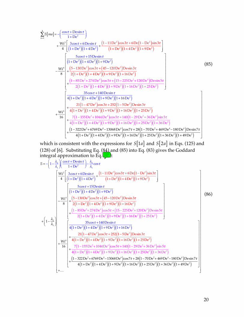
which is consistent with the expressions for S 1a[ ] and S 2a[ ] in Eqs. (125) and (128) of [6]. Substituting Eq. (84) and (85) into Eq. (83) gives the Goddard integral approximation to Eq. (14):
S = − 1−λ2
λ1
⎛⎝⎜
⎞⎠⎟
cosτ + Desinτ1+ De2
⎛⎝⎜
⎞⎠⎟−λ2
λ1
cosτ
+ 1−λ2
λ1
⎛⎝⎜
⎞⎠⎟
Wi2
43cosτ + 6Desinτ1+ De2( ) 1+ 4 De2( ) +
1−11De2( )cos3τ + 6De 1− De2( )sin 3τ1+ De2( ) 1+ 4 De2( ) 1+ 9De2( )
⎡
⎣⎢⎢
⎤
⎦⎥⎥
− Wi4
8
5cosτ +15Desinτ1+ De2( ) 1+ 4 De2( ) 1+ 9De2( )+
5−130De2( )cos3τ + 45−120De2( )Desin 3τ2 1+ De2( ) 1+ 4 De2( ) 1+ 9De2( ) 1+16De2( )
+1− 85De2+ 274 De4( )cos5τ + 15− 225De2+120De4( )Desin 5τ
2 1+ De2( ) 1+ 4 De2( ) 1+ 9De2( ) 1+16De2( ) 1+ 25De2( )
⎡
⎣
⎢⎢⎢⎢⎢⎢⎢⎢⎢
⎤
⎦
⎥⎥⎥⎥⎥⎥⎥⎥⎥
+ Wi6
16
35cosτ +140Desinτ4 1+ De2( ) 1+ 4 De2( ) 1+ 9De2( ) 1+16De2( )+
21 1− 47 De2( )cos3τ + 252 1− 5De2( )Desin 3τ4 1+ De2( ) 1+ 4 De2( ) 1+ 9De2( ) 1+16De2( ) 1+ 25De2( )
+7 1−155De2+1044 De4( )cos5τ +140 1− 29De2+ 36De4( )sin 5τ
4 1+ De2( ) 1+ 4 De2( ) 1+ 9De2( ) 1+16De2( ) 1+ 25De2( ) 1+ 36De2( )+
1− 322De2+ 6769De4−13068De6( )cos7τ + 28 1− 70De2+ 469De4−180De6( )Desin7τ4 1+ De2( ) 1+ 4 De2( ) 1+ 9De2( ) 1+16De2( ) 1+ 25De2( ) 1+ 36De2( ) 1+ 49De2( )
⎡
⎣
⎢⎢⎢⎢⎢⎢⎢⎢⎢⎢⎢⎢
⎤
⎦
⎥⎥⎥⎥⎥⎥⎥⎥⎥⎥⎥⎥
+…
⎡
⎣
⎢⎢⎢⎢⎢⎢⎢⎢⎢⎢⎢⎢⎢⎢⎢⎢⎢⎢⎢⎢⎢⎢⎢⎢⎢⎢⎢⎢⎢
⎤
⎦
⎥⎥⎥⎥⎥⎥⎥⎥⎥⎥⎥⎥⎥⎥⎥⎥⎥⎥⎥⎥⎥⎥⎥⎥⎥⎥⎥⎥⎥
(86)

21
which we will next use to validate our main result. The accuracies of Eqs. (85) and (86) can improve with the use of Padé approximants [47], though we found no need for this here (see Figure 6 through Figure 9).
When the Wi6 term is omitted, Eq. (86) reduces to Eq. (58) of [6] as it must. To our knowledge, Eq. (86) is new. Since our exact solution does not take the form of a Fourier series, Eq. (86) is thus, to our knowledge, the first expression for each of the shear stress harmonics for the corotational Jeffreys fluid up to the seventh. Figure 6 through Figure 9 show that Eq. (86) agrees closely, well within a pen width, with our new exact solution, Eq. (60) [with Eqs. (61) and (62)].
ii. Finite Difference Solution Viscoelastic models in large-amplitude oscillatory shear flow can also be
solved approximately numerically by the finite element method [48,49], or by numerical integration [50,51,52,53,54], or by finite difference [55,56,57,58,59,60, 61,62,63,64,65,66,67,68,69,70,71,72,73,74,75,76,77,78,79,80,81]. Here, as a consistency check on Eq. (60), we use the Runge-Kutta 5(4) finite difference scheme [82] to solve Eqs. (41)–(43) for the shear stress subject to the initial conditions:
S 0( ) = N1 0( ) = N2 0( ) = 0 (87)
Our computation is, of course, independent of ⌣τ zz 0( ) , since for the corotational
Jeffreys model, ν1 = ν2 = 0 , or since because for the corotational Jeffreys model
µ0 = 23 µ1 = 0 . The conditions ν1 = ν2 = 0 or µ0 = 2
3 µ1 = 0 satisfy Eqs. (75) and (76), our conditions for
⌣τ zz invariance. For our finite difference solution to Eqs. (41)–(43) subject to Eq. (87), we
coded into MATLAB (Version R2012b) on a MacBook Air (1.3 GHz Intel Core i5 processor with 4 GB 1600 MHz DDR3 memory) employing the OS X (Version 10.10.2) operating system using the ode45 scheme. For each point in Figure 10 through Figure 12, we find such an evaluation to consume less than 1 second of CPU time. Figure 10 through Figure 12 show the consistency between our numerical and exact solutions, well within a pen width, for the Oldroyd 8-constant framework in large-amplitude oscillatory shear flow. Indeed, we find that our finite difference and exact solutions agree to at least within 16 significant figures. V. WORKED EXAMPLE: η∞ AND THE HIGHER HARMONICS
In this section, we illustrate the use of our exact solution for the Oldroyd 8-constant framework in LAOS [Eq. (60) with Eqs. (61) and (62)]. Specifically, we use our exact solution to explore the role of η∞ on the higher harmonics of the shear stress. For this exploration, we choose the special case of the corotational
22
Jeffreys model, the simplest relevant model containing η∞ . By relevant, we still mean that the model at least predicts higher shear stress harmonics. More specifically, for the corotational Jeffreys model, η∞ η0 = λ2 λ1 [see Eq. (28)].
Figure 6 through Figure 9 employ Eq. (60) with Eqs. (61) and (62) to illustrate the role of η∞ on the loop shapes. Comparing Figure 6 with successively Figure 7 through Figure 9, we learn that increasing η∞ narrows the shear stress versus shear rate loops, and thus diminishes their areas. In other words, increasing η∞ decreases fluid elasticity, and increases viscous dissipation [17,18, 19]. From Figure 6 through Figure 9, we see that increasing η∞ does not produce self-intersection, at least not over the ranges
110 < Wi < 5
4 and 0.1 < De < 10 [83]. VI. CONCLUSION
In this work, we arrive at the first exact analytical solution [Eq. (60) with Eqs. (61) and (62)] to a framework of constitutive equations for LAOS. We chose the Oldroyd 8-constant framework for a rich of diversity of popular constitutive equations. To our knowledge, our exact analytical solution [Eq. (60) with Eqs. (61) and (62)] is the first exact solution to a framework of constitutive equation in LAOS. Our new exact analytical solution reduces to our previous result for the corotational Maxwell fluid (Eq. (62) with Eqs. (127) and (134) of [9]), as it should.
To our knowledge, our Subsection IV.c.i provides the first integral expansion to the corotational Jeffreys fluid [Eq. (86)], by following the method in Section 8. of [6], and this up to and including the seventh harmonic. We use this Eq. (86) to validate our main result [Eq. (60) with Eqs. (61) and (62)] for the special case of the corotational Jeffreys fluid in LAOS.
To arrive at Eq. (86), obtained Eq. (85), the integral expansion to the corotational Maxwell fluid. Eq. (85) extends Eq. (58) of [6] to the next term, that is, to the sixth order of Wi .
Some special cases of the Oldroyd 8-constant framework (corotational Maxwell or corotational Jeffreys), are used with multiple relaxation times, λ1 . Extending the results of this work to multiple λ1 might thus be a useful next step, and for this, we would begin with the Spriggs relations (see Eqs. (6.1-14) and (6.1-15) of [21]; see also Appendix of [40]). Other special cases of the Oldroyd 8-constant framework (Johnson-Segalman or Gordon-Schowalter) are often useful without extension to multiple λ1 .
In this paper, we have limited the scope to just the alternant part of the shear stress in LAOS. Previously, for the exact solution to the corotational Maxwell model, we solved exactly for both the shear stress and the normal stress

23
differences, and these for both start-up and alternance, using the Kovacic method [9]. We, of course, expect start-up and the normal stress differences for the Oldroyd 8-constant framework to yield to the Kovacic method. However, for the Oldroyd 8-constant framework, we leave the exact solution for start-up and for the normal stress differences for another day.
In our previous work, we succeeded in rewriting our exact solutions for the corotational Maxwell fluid (Eq. (62) with Eqs. (127) and (134) of [9]) as a Fourier series (Eq. (66) of [9]). However, in this work, we have yet to rewrite our main result [Eq. (60) with Eqs. (61) and (62)] as a Fourier series. This too we shall leave for another day.
We have a strong preference for the approach that we have taken in this paper, which produces the exact solution for an entire framework, over the approach in Ref. [9], which produces an exact solution for just one constitutive equation. We prefer the framework approach because it at once generates exact solutions in LAOS to whole sets of constitutive equations, rather than generating solutions for one constitutive equation at a time.
VII. ACKNOWLEDGMENT
A.J. Giacomin is indebted to the Faculty of Applied Science and Engineering of Queen’s University at Kingston, for its support through a Research Initiation Grant (RIG). This research was undertaken, in part, thanks to support from the Canada Research Chairs program of the Government of Canada for the Natural Sciences and Engineering Research Council of Canada (NSERC) Tier 1 Canada Research Chair in Rheology. This research was also undertaken, in part, thanks to support from the Discovery Grant program of the Natural Sciences and Engineering Research Council of Canada (NSERC).
We thank the Royal Golden Jubilee Program of the Thailand Research Fund for a grant (Contract No. PHD/0116/2554). We publish this paper in remembrance of His Majesty King Bhumibol Adulyadej 1927–2016.
VIII. APPENDICES
a. Deriving Four Differential Equations in S , N1 , N2 and ⌣τ zz
In this Appendix, we will derive four the differential equation in S , N1 , N2 and
⌣τ zz from Eq. (14). To prepare for this derivation, we first substitute Eqs. (12) and (13) into Eqs. (20) and (21) to get:
D τD t
≡ ∂∂t
τ xx τ xy τ xz
τ yx τ yy τ yz
τ zx τ zy τ zz
⎡
⎣
⎢⎢⎢⎢
⎤
⎦
⎥⎥⎥⎥
+ 12!γ
−2τ yx τ xx −τ yy 0τ xx −τ yy 2τ yx 0
0 0 0
⎡
⎣
⎢⎢⎢⎢
⎤
⎦
⎥⎥⎥⎥
(88)
and:

24
D !γD t
≡ ∂∂t!γ
0 1 01 0 00 0 0
⎡
⎣
⎢⎢⎢
⎤
⎦
⎥⎥⎥+ !γ 2
−1 0 00 1 00 0 0
⎡
⎣
⎢⎢⎢
⎤
⎦
⎥⎥⎥
(89)
We next use Eq. (11) to rewrite the third term on the left of Eq. (14) as:
12µ0 tr τ( ) !γ = 1
2µ0 τ xx +τ yy +τ zz( ) !γ
0 1 01 0 00 0 0
⎡
⎣
⎢⎢⎢
⎤
⎦
⎥⎥⎥
(90)
and the fourth:
− 12µ1 τ ⋅ !γ + !γ ⋅ τ{ } = − 1
2µ1 !γ
2τ yx τ xx +τ yy τ yz
τ xx +τ yy 2τ yx τ xz
τ yz τ zx 0
⎡
⎣
⎢⎢⎢⎢
⎤
⎦
⎥⎥⎥⎥
(91)
and the last:
12ν1 τ : !γ( )δ = ν1τ yx !γ
1 0 00 1 00 0 1
⎡
⎣
⎢⎢⎢
⎤
⎦
⎥⎥⎥
(92)
Using Eq. (11) to rewrite the third term on the right of Eq. (14), we get:
−µ2 !γ ⋅ !γ{ } = −µ2 !γ2
1 0 00 1 00 0 0
⎡
⎣
⎢⎢⎢
⎤
⎦
⎥⎥⎥
(93)
and to rewrite the last:
12ν2 !γ : !γ( )δ = ν2 !γ
21 0 00 1 00 0 1
⎡
⎣
⎢⎢⎢
⎤
⎦
⎥⎥⎥
(94)
Substituting Eqs. (88) through (94) into Eq. (14) gives:
τ xx τ yx τ xz
τ yx τ yy τ yz
τ xz τ yz τ zz
⎡
⎣
⎢⎢⎢⎢
⎤
⎦
⎥⎥⎥⎥
+ λ1∂∂t
τ xx τ yx τ xz
τ yx τ yy τ yz
τ xz τ yz τ zz
⎡
⎣
⎢⎢⎢⎢
⎤
⎦
⎥⎥⎥⎥
+ 12!γ
−2τ yx τ xx −τ yy 0τ xx −τ yy 2τ yx 0
0 0 0
⎡
⎣
⎢⎢⎢⎢
⎤
⎦
⎥⎥⎥⎥
⎛
⎝
⎜⎜⎜⎜
⎞
⎠
⎟⎟⎟⎟
+ 12µ0 τ xx +τ yy +τ zz( ) !γ
0 1 01 0 00 0 0
⎡
⎣
⎢⎢⎢
⎤
⎦
⎥⎥⎥− 1
2µ1 !γ
2τ yx τ xx +τ yy τ yz
τ xx +τ yy 2τ yx τ xz
τ yz τ zx 0
⎡
⎣
⎢⎢⎢⎢
⎤
⎦
⎥⎥⎥⎥
+ν1τ yx !γ1 0 00 1 00 0 1
⎡
⎣
⎢⎢⎢
⎤
⎦
⎥⎥⎥
= −η0 !γ0 1 01 0 00 0 0
⎡
⎣
⎢⎢⎢
⎤
⎦
⎥⎥⎥−η0λ2
∂∂t!γ
0 1 01 0 00 0 0
⎡
⎣
⎢⎢⎢
⎤
⎦
⎥⎥⎥+ !γ 2
−1 0 00 1 00 0 0
⎡
⎣
⎢⎢⎢
⎤
⎦
⎥⎥⎥
⎛
⎝
⎜⎜
⎞
⎠
⎟⎟ +η0µ2 !γ
21 0 00 1 00 0 0
⎡
⎣
⎢⎢⎢
⎤
⎦
⎥⎥⎥−η0ν2 !γ
21 0 00 1 00 0 1
⎡
⎣
⎢⎢⎢
⎤
⎦
⎥⎥⎥
(95)
which we will use to get τ yx , N1 , N2 and τ zz (or, in dimensionless form, S , N1 ,
N2 and ⌣τ zz ).
The yx, xx, yy and zz-component of Eq. (95) are:

25
1+ λ1∂∂t
⎛⎝⎜
⎞⎠⎟τ yx +
12
λ1 − µ1 + µ0( )τ xx !γ − 12
λ1 + µ1 − µ0( )τ yy !γ + 12µ0τ zz !γ
= −η0 1+ λ2∂∂t
⎛⎝⎜
⎞⎠⎟!γ
(96)
1+ λ1
∂∂t
⎛⎝⎜
⎞⎠⎟τ xx − λ1 + µ1 −ν1( )τ yx !γ =η0 λ2 + µ2 −ν2( ) !γ 2 (97)
1+ λ1
∂∂t
⎛⎝⎜
⎞⎠⎟τ yy + λ1 − µ1 +ν1( )τ yx !γ = −η0 λ2 − µ2 +ν2( ) !γ 2 (98)
1+ λ1
∂∂t
⎛⎝⎜
⎞⎠⎟τ zz +ν1τ yx !γ = −η0ν2 !γ
2 (99)
which match Eqs. (8.1-3)–(8.1-6) of [21]. We next rewrite these four differential equations in terms of the first and second normal stress differences as:
1+ λ1∂∂t
⎛⎝⎜
⎞⎠⎟τ yx +
12
λ1 − µ1 + µ0( )N1 !γ − µ1 − µ0( )N2 !γ + 32µ0 − µ1
⎛⎝⎜
⎞⎠⎟τ zz !γ
= −η0 1+ λ2∂∂t
⎛⎝⎜
⎞⎠⎟!γ
(100)
1+ λ1
∂∂t
⎛⎝⎜
⎞⎠⎟
N1 − 2λ1τ yx !γ = 2λ2η0 !γ2 (101)
1+ λ1
∂∂t
⎛⎝⎜
⎞⎠⎟
N2 + λ1 − µ1( )τ yx !γ = −η0 λ2 − µ2( ) !γ 2 (102)
Substituting the yx-component in Eq. (11) into Eqs. (99)–(102) gives Eqs. (37)–(44) above.
We next turn our attention to the two remaining components of extra stress tensor. The xz and yz-components of Eq. (95) are:
τ xz + λ1
∂∂tτ xz −
12µ1τ yz !γ = 0 (103)
τ yz + λ1
∂∂tτ yz −
12µ1τ xz !γ = 0 (104)
Solving Eqs. (103) and (104) subject to the initial conditions:
τ yz 0( ) = τ xz 0( ) = 0 (105) gives:
τ xz t( ) = τ yz t( ) = 0 (106)
from which we confirm that τ xz t( ) and τ yz t( ) make no contribution to simple shear flow.
For the special case of corotational Maxwell fluid, where
λ2 = µ0 = µ1 = µ2 = ν1 = ν2 = 0 , Eqs. (41)–(43) reduce to:

26
dN1
dτ= − 1
DeN1 + 2
WiDe
Scosτ (107)
dN2
dτ= − 1
DeN2 −
WiDe
Scosτ (108)
dSdτ
= − 12
WiDe
N1 cosτ − 1De
S − 1De
cosτ (109)
which match Eqs. (32), (33) and (36) in [9], which serves as an intermediate consistency check.
b. Solving Eqs. (46)–(49) by the Kovacic Method Differentiating Eq. (49) once gives:
d2Sdτ 2 = − 1
21−
µ1
λ1
+µ0
λ1
⎛⎝⎜
⎞⎠⎟
WiDe
dN1
dτcosτ −N1 sinτ⎛
⎝⎜⎞⎠⎟+
µ1
λ1
−µ0
λ1
⎛⎝⎜
⎞⎠⎟
WiDe
dN2
dτcosτ −N2 sinτ⎛
⎝⎜⎞⎠⎟
− 32µ0
λ1
−µ1
λ1
⎛⎝⎜
⎞⎠⎟
WiDe
d⌣τ zz
dτcosτ − ⌣τ zz sinτ⎛
⎝⎜⎞⎠⎟− 1
DedSdτ
(110)
Substituting Eq. (48) into Eq. (110) and rearranging gives:
d2Sdτ 2 = − 1
21−
µ1
λ1
+µ0
λ1
⎛⎝⎜
⎞⎠⎟
WiDe
dN1
dτcosτ −N1 sinτ⎛
⎝⎜⎞⎠⎟+
µ1
λ1
−µ0
λ1
⎛⎝⎜
⎞⎠⎟
WiDe
dN2
dτcosτ −N2 sinτ⎛
⎝⎜⎞⎠⎟
+ 32µ0
λ1
−µ1
λ1
⎛⎝⎜
⎞⎠⎟
Wi2
De2
ν1
λ1
Scos2τ − 1De
dSdτ
+ 32µ0
λ1
−µ1
λ1
⎛⎝⎜
⎞⎠⎟
WiDe
1De
cosτ + sinτ⎡⎣⎢
⎤⎦⎥⌣τ zz
(111)
Solving Eq. (49) gives:
32µ0
λ1
−µ1
λ1
⎛⎝⎜
⎞⎠⎟
WiDe⌣τ zz = − 1
cosτdSdτ
− 12
1−µ1
λ1
+µ0
λ1
⎛⎝⎜
⎞⎠⎟
WiDe
N1 +µ1
λ1
−µ0
λ1
⎛⎝⎜
⎞⎠⎟
WiDe
N2 −1
DeS
cosτ (112)
Substituting Eq. (112) into Eq. (111), and then, Eqs. (46) and (47) into the result gives:
d2Sdτ 2 +
2De
+ tanτ⎛⎝⎜
⎞⎠⎟
dSdτ
+ 1De2 +
tanτDe
+ 1+µ0
λ1
µ1
λ1
− 32ν1
λ1
⎛⎝⎜
⎞⎠⎟−µ1
λ1
µ1
λ1
−ν1
λ1
⎛⎝⎜
⎞⎠⎟
⎡
⎣⎢
⎤
⎦⎥
Wi2
De2 cos2τ⎡
⎣⎢⎢
⎤
⎦⎥⎥S = 0 (113)
Solving Eq. (113) using the Kovacic method (see Section 4.1 of [14]; Appendix: Fundamental Matrix of [9]), we first discover that a solution to Eq. (14) will both exist and be in closed form, and then that this solution will be unique. Proceeding then with the solution to Eq. (113) gives Eq. (50) above.
Substituting Eq. (50) into Eqs. (46) and (47) gives:
dN1
dτ= − 1
DeN1 + 2
WiDe
C1e−τ De sin α sin( ) +C2e
−τ De cos α sin( )⎡⎣ ⎤⎦cosτ (114)
and:
dN2
dτ= − 1
DeN2 − 1−
µ1
λ1
⎛⎝⎜
⎞⎠⎟
WiDe
C1e−τ De sin α sinτ( ) +C2e
−τ De cos α sinτ( )⎡⎣ ⎤⎦cosτ (115)
27
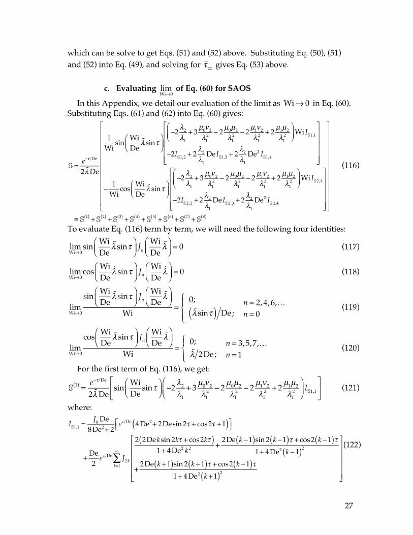
which can be solve to get Eqs. (51) and (52) above. Substituting Eq. (50), (51) and (52) into Eq. (49), and solving for
⌣τ zz gives Eq. (53) above.
c. Evaluating limWi→0
of Eq. (60) for SAOS
In this Appendix, we detail our evaluation of the limit as Wi→ 0 in Eq. (60). Substituting Eqs. (61) and (62) into Eq. (60) gives:
S = e−τ De
2 !λ De
1Wi
sinWiDe!λ sinτ⎛
⎝⎜⎞⎠⎟
−2λ2
λ1
+ 3µ0ν2
λ12 − 2
µ0µ2
λ12 − 2
µ1ν2
λ12 + 2
µ1µ2
λ12
⎛⎝⎜
⎞⎠⎟
Wi IS1,1
−2IS1,2 + 2λ2
λ1
DeIS1,3 + 2λ2
λ1
De2 IS1,4
⎡
⎣
⎢⎢⎢⎢⎢
⎤
⎦
⎥⎥⎥⎥⎥
− 1Wi
cosWiDe!λ sinτ⎛
⎝⎜⎞⎠⎟
−2λ2
λ1
+ 3µ0ν2
λ12 − 2
µ0µ2
λ12 − 2
µ1ν2
λ12 + 2
µ1µ2
λ12
⎛⎝⎜
⎞⎠⎟
Wi IS2,1
−2IS2,2 + 2λ2
λ1
DeIS2,3 + 2λ2
λ1
De2 IS2,4
⎡
⎣
⎢⎢⎢⎢⎢
⎤
⎦
⎥⎥⎥⎥⎥
⎡
⎣
⎢⎢⎢⎢⎢⎢⎢⎢⎢⎢⎢
⎤
⎦
⎥⎥⎥⎥⎥⎥⎥⎥⎥⎥⎥
≡ S 1( ) + S 2( ) + S 3( ) + S 4( ) + S 5( ) + S 6( ) + S 7( ) + S 8( )
(116)
To evaluate Eq. (116) term by term, we will need the following four identities:
limWi→0
sin WiDe!λ sinτ⎛
⎝⎜⎞⎠⎟
JnWiDe!λ⎛
⎝⎜⎞⎠⎟= 0 (117)
limWi→0
cosWiDe!λ sinτ⎛
⎝⎜⎞⎠⎟
JnWiDe!λ⎛
⎝⎜⎞⎠⎟= 0 (118)
limWi→0
sin WiDe!λ sinτ⎛
⎝⎜⎞⎠⎟
JnWiDe!λ⎛
⎝⎜⎞⎠⎟
Wi=
0;!λ sinτ( ) De;
n = 2,4,6,…n = 0
⎧⎨⎪
⎩⎪ (119)
limWi→0
cosWiDe!λ sinτ⎛
⎝⎜⎞⎠⎟
JnWiDe!λ⎛
⎝⎜⎞⎠⎟
Wi=
0;!λ 2De;
n = 3,5,7,…n = 1
⎧⎨⎪
⎩⎪ (120)
For the first term of Eq. (116), we get:
S 1( ) = e−τ De
2 !λ Desin Wi
Desinτ⎛
⎝⎜⎞⎠⎟
−2 λ2
λ1+ 3 µ0ν2
λ12 − 2 µ0µ2
λ12 − 2 µ1ν2
λ12 + 2 µ1µ2
λ12
⎛⎝⎜
⎞⎠⎟
IS1,1
⎡
⎣⎢
⎤
⎦⎥ (121)
where:
IS1,1 =J0 De
8De2+ 2eτ De 4 De2+ 2Desin 2τ + cos2τ +1( )⎡⎣ ⎤⎦
+ De2
eτ De J2k
2 2Deksin 2kτ + cos2kτ( )1+ 4 De2 k2 +
2De k −1( )sin 2 k −1( )τ + cos2 k −1( )τ1+ 4 De2 k −1( )2
+2De k +1( )sin 2 k +1( )τ + cos2 k +1( )τ
1+ 4 De2 k +1( )2
⎡
⎣
⎢⎢⎢⎢⎢
⎤
⎦
⎥⎥⎥⎥⎥
k=1
∞
∑(122)

28
where Jm ≡ Jm α( ) is the mth order Bessel function of the first kind (see after Eq. (5) of [44] or before Eq. (123) of [9]). Using Eq. (117) to simplify Eq. (122) gives:
S 1( ) = 0 (123) For the second term of Eq. (116), we get:
S 2( ) = e−τ De
2 !λ De1
Wisin Wi
Desinτ⎛
⎝⎜⎞⎠⎟−2IS1,2⎡⎣ ⎤⎦
⎡
⎣⎢
⎤
⎦⎥ (124)
where:
IS1,2 = J0 Deeτ De +
2De J2keτ De
4 De2 k2 +1cos2kτ + 2k Desin 2kτ( )
k=1
∞
∑ (125)
and using Eq. (119) then gives:
S 2( ) = − sinτ
De (126)
For the third term of Eq. (116), we get:
S 3( ) = e−τ De
2 !λ De1
Wisin Wi
Desinτ⎛
⎝⎜⎞⎠⎟
2 λ2
λ1DeIS1,3
⎡
⎣⎢
⎤
⎦⎥
⎡
⎣⎢
⎤
⎦⎥ (127)
where:
IS1,3 = i De J0 −eτ De + 2eτ De2F1 1,− i
2De;1− i
2De;−e2 iτ⎛
⎝⎜⎞⎠⎟
⎡
⎣⎢
⎤
⎦⎥
+2De J2k
eτ De
1+ 4k2 De2 −sin 2kτ + 2k Decos2kτ( ) + i −1( )1+k eτ De
−−1( )1−l+k
2eτ De
1+ 4l2 De2 sin 2lτ − 2l Decos2lτ( )⎡
⎣⎢⎢
⎤
⎦⎥⎥l=1
k
∑
+2i −1( )k eτ De2F1 1,− i
2De;1− i
2De;−e2 iτ⎛
⎝⎜⎞⎠⎟
⎡
⎣
⎢⎢⎢⎢⎢⎢⎢⎢
⎤
⎦
⎥⎥⎥⎥⎥⎥⎥⎥
k=1
∞
∑ (128)
and using Eq. (119), we then get:
S 3( ) =
λ2
λ1isinτ −1+ 2 2F1 1,− i
2De;1− i
2De;−e2 iτ⎛
⎝⎜⎞⎠⎟
⎡
⎣⎢
⎤
⎦⎥ (129)
For the fourth term of Eq. (116):
S 4( ) = e−τ De
2 !λ De1
Wisin Wi
Desinτ⎛
⎝⎜⎞⎠⎟
2 λ2
λ1De2 IS1,4
⎡
⎣⎢
⎤
⎦⎥
⎡
⎣⎢
⎤
⎦⎥ (130)
where:

29
IS1,4 = 2iJ0
eτ De
ei2τ +1− eτ De
2F1 1,− i2De
;1− i2De
;−ei2τ⎛⎝⎜
⎞⎠⎟
⎡
⎣⎢
⎤
⎦⎥
+2 J2kk=1
∞
∑
−1( )k2k Deeτ De + −1( )k i 2eτ De
ei2τ +1⎛⎝⎜
⎞⎠⎟
+4eτ De De−1( )k−m k − m+1( )
1+ 4 m−1( )2De2
cos2 m−1( )τ+2 m−1( )Desin 2 m−1( )τ⎡
⎣⎢⎢
⎤
⎦⎥⎥m=1
k
∑
−2i −1( )k eτ De2F1 1,− i
2De;1− i
2De;−ei2τ⎛
⎝⎜⎞⎠⎟
⎡
⎣
⎢⎢⎢⎢⎢⎢⎢⎢
⎤
⎦
⎥⎥⎥⎥⎥⎥⎥⎥
(131)
and using Eq. (119) then gives:
S 4( ) =2 λ2
λ1isinτ 1
ei2τ +1− 2F1 1,− i
2De;1− i
2De;−ei2τ⎛
⎝⎜⎞⎠⎟
⎡
⎣⎢
⎤
⎦⎥ (132)
For the fifth term of Eq. (116), we get:
S 5( ) = e−τ De
2 !λ De−cos
WiDe
sinτ⎛⎝⎜
⎞⎠⎟
−2λ2
λ1
+ 3µ0ν2
λ12 − 2
µ0µ2
λ12 − 2
µ1ν2
λ12 + 2
µ1µ2
λ12
⎛⎝⎜
⎞⎠⎟
IS2,1
⎡
⎣⎢
⎤
⎦⎥ (133)
where:
IS2,1 = 2 J2k−1
− 1+ 2k( )De2 eτ De cos 1+ 2k( )τ4 1+ De2 1+ 2k( )2( ) +
3− 2k( )De2 eτ De cos 3− 2k( )τ4 1+ De2 3− 2k( )2( )
+De2 1− 2k( )eτ De cos 1− 2k( )τ
2 1+ De2 1− 2k( )2( )+Deeτ De sin 1+ 2k( )τ
4 1+ De2 1+ 2k( )2( ) −sin 1− 2k( )τ
2 1+ De2 1− 2k( )2( ) −sin 3− 2k( )τ
4 1+ De2 3− 2k( )2( )⎡
⎣
⎢⎢⎢
⎤
⎦
⎥⎥⎥
⎡
⎣
⎢⎢⎢⎢⎢⎢⎢⎢⎢⎢⎢⎢
⎤
⎦
⎥⎥⎥⎥⎥⎥⎥⎥⎥⎥⎥⎥
k=1
∞
∑ (134)
and using Eq. (118) then gives:
S 5( ) = 0 (135) For the sixth term of Eq. (116), we get:
S 6( ) = e−τ De
2 !λ De− 1
Wicos
WiDe
sinτ⎛⎝⎜
⎞⎠⎟
−2IS2,2⎡⎣ ⎤⎦⎡
⎣⎢
⎤
⎦⎥ (136)
where:
IS2,2 = 2De J2k−1
eτ De 1− 2k( )Decos 1− 2k( )τ − sin 1− 2k( )τ⎡⎣ ⎤⎦1+ De2 1− 2k( )2
k=1
∞
∑ (137)
and using Eq. (120) then gives:
S 6( ) = −Decosτ + sinτ
De 1+ De2( ) (138)
For the seventh term of Eq. (116), we get:

30
S 7( ) = e−τ De
2 !λ De− 1
Wicos
WiDe
sinτ⎛⎝⎜
⎞⎠⎟
2λ2
λ1
DeIS2,3
⎡
⎣⎢
⎤
⎦⎥
⎡
⎣⎢
⎤
⎦⎥ (139)
where:
IS2,3 = 2 J2k−1
Deeτ De cos 2k −1( )τ + 2k −1( )Desin 2k −1( )τ⎡⎣ ⎤⎦1+ 2k −1( )2
De2
+2Deeτ De −1( )k−n+1cos 2n−1( )τ + 2n−1( )Desin 2n−1( )τ⎡⎣ ⎤⎦
1+ 2n−1( )2De2
n=1
k
∑
+−1( )k+1
2De1+ i De( ) eτ Deeiτ
2F1 1,12− i
2De;32− i
2De;−ei2τ⎛
⎝⎜⎞⎠⎟
⎡
⎣
⎢⎢⎢⎢⎢⎢⎢⎢⎢
⎤
⎦
⎥⎥⎥⎥⎥⎥⎥⎥⎥
k=1
∞
∑ (140)
and using Eq. (120) then gives:
S 7( ) =
λ2
λ1
cosτ + Desinτ1+ De2 − 2eiτ
1+ i De( ) 2F1 1,12− i
2De;32− i
2De;−ei2τ⎛
⎝⎜⎞⎠⎟
⎡
⎣⎢
⎤
⎦⎥ (141)
For the eighth term of Eq. (116), we get:
S 8( ) = e−τ De
2 !λ De− 1
Wicos
WiDe
sinτ⎛⎝⎜
⎞⎠⎟
2λ2
λ1
De2 IS2,4
⎡
⎣⎢
⎤
⎦⎥
⎡
⎣⎢
⎤
⎦⎥ (142)
where:
IS2,4 = 2 J2k−1
−1( )k−m−14 De k − m( )eτ De
1+ 2m−1( )2De2
sin 2m−1( )τ− 2m−1( )Decos 2m−1( )τ⎡
⎣⎢⎢
⎤
⎦⎥⎥m=1
k
∑
+ −1( )k+1 eτ De secτ −2i −1( )k+1
i − Dee 1 De+i( )τ
2F1 1,12− i
2De;32− i
2De;−ei2τ⎛
⎝⎜⎞⎠⎟
⎡
⎣
⎢⎢⎢⎢⎢
⎤
⎦
⎥⎥⎥⎥⎥
k=1
∞
∑ (143)
and using Eq. (120) then gives:
S 8( ) =
−λ2
λ1secτ − i2eiτ
i − De 2F1 1, 12− i
2De; 32− i
2De;−ei2τ⎛
⎝⎜⎞⎠⎟
⎡
⎣⎢
⎤
⎦⎥ (144)
Substituting Eqs. (123), (126), (129), (132), (135), (138), (141) and (144) back into Eq. (116) gives Eq. (78) above.

31
Table I: Literature on Analytical Solutions for Large-Amplitude Oscillatory Shear Flow
Authors (year)
Mod
el
Shear Stress
Harmonic
Normal Stress Difference Harmonic
Orie
ntat
ion
Star
tup
Form
[Ref
.] (C
orre
ctio
n to
)
Firs
t
Third
Fifth
Zero
th
Seco
nd
Four
th
Kirkwood and Plock (1956, 1967); Plock (1957)
RD h , SK h
n ψ ≅ [84,85,86]
Lodge (1961, 1964) L✝ N1 N1
= [87,88]
Spriggs (1966) NGJ N1 N1
= [89]
Spriggs (1966) CJ N
1
N2
N
1
N2
= [89]
Williams and Bird (1962) O3 N1
= [90] Williams and Bird (1964) O3 N1
N1 = [91]
Spriggs (1965) O3✝
N
1
N2
N
1
N2
= [92]
Akers and Williams (1969) RZ N1
N1
= [93]
Paul (1969); Paul (1970); Bharadwaj (2012)
RD h , SK h
n X ψ ≅ [94,95,96] (84,86)
Walters and Jones (1970); Walters (1975) I3 n X ≅
[97]; Section 6.2.3 of [98]
Paul and Mazo (1969), Paul (1970) RR n X ψ ≅ [99,95]
MacDonald, Marsh and Ashare (1969)
BC, OWFS✝ n ≅ [50]
Bird, Warner and Evans (1971) RD n
N
1
N2
N
1
N2
ψ ≅ [100]
Leal and Hinch (1972) RSD N
1
N2
N1
N2
ψ ≅ Section 3.3 of [101]
Abdel-Khalik et al. (1974); Bird et al. (1974) GE+SK n
N
1
N2
N
1
N2
≅ [23,24]
Bird et al. (1977) BHS 0 0 ψ = Table 11.4-2 [102]
Mou and Mazo (1977) RR N
1
N2
N1
N2
ψ ≅ [103](99)
Pearson and Rochefort (1982); Helfand and Rochefort (1982)
R✝ n X ≅ [104,105]

32
Fan and Bird (1984) CB✝ n X ≅ [106](105)
Oakley (1992); Oakley and Giacomin (1994) L✝ N1
N1 =
APPENDIX B of [107]; [108](87)
Phan-Thien et al. (2000) Dough = [109] Yu et al. (2002); Zhou (2004) SE n X N1
N1 N1
≅ [110,111]
Cho et al. (2010) K-BKZ [16] Hoyle (2010) PP n ≅ Ch. 4 of [112] Wagner et al. (2011) R n X ≅ [113]
Giacomin et al. (2011) CM✝, CJ n X X
N
1
N2
N
1
N2
N
1
N2
X ≅ [6] (114)
Giacomin and Bird (2011) ANSR n X X
N
1
N2
N1
N2
N1
N2
X ≅ [115]
Gurnon and Wagner (2012) G X
N
1
N2
N1
N2
≅ [116]
Bird et al. (2014) RD n X ψ ≅ [117]
Schmalzer et al. (2014) RD N
1
N2
N
1
N2
N
1
N2
ψ ≅ [118,119](6,115); [120]
Thompson and de Souza Mendes (2015) MSJ n 0 0 0 0 ≅
See Section 5.2.2 of [121]
Bozorgi (2014); Bozorgi and Underhill (2014) AS h n X ψ ≅
Ch. 8 of [122]; [123]
Blackwell (2014) CJ ξ X ≅ [124] Giacomin et al. (2015) RD ψ ≅ [125]
Giacomin et al. (2015) CM n X X N
1
N2
N1
N2
N1
N2
X ≅ [47]
Saengow et al. (2015) CM✝ n X X N
1
N2
N1
N2
N1
N2
X = [9]
Merger el al. (2016) MCM n X = [126,127]
This paper O8 n X X = [128] Legend: ANSR ≡ corotational arbitrary normal stress ratio; AS ≡ active rod suspensions; BC ≡ Bird-Carreau; BHS ≡ Bead-Hookean spring; CB ≡ Curtiss-Bird; CJ ≡ corotational Jeffreys; CM ≡ corotational Maxwell; G ≡ Giesekus; GE ≡ Goddard integral expansion; I3 ≡ third order integral; K-BKZ ≡ Kaye-Bernstein, Kearsley, Zappas; L ≡ Lodge rubberlike; M ≡ Maxwell fluid; MSJ ≡ material subjective Jeffreys; NGJ ≡ nonlinear Generalized Jeffreys; O3 ≡ Oldroyd 3-constant; OWFS ≡ modified Oldroyd-Walters-Fredrickson-Spriggs; O8 ≡ Oldroyd 8-constant; P ≡ Padé approximants; PP ≡ pompom; R ≡ reptation; RD ≡ rigid dumbbell; RR ≡ planar rigid ring; RSD ≡ rods, spheres or disks; RZ ≡ Rouse-Zimm; SE ≡ simple emulsion; SK ≡ shish-kebab; N1 ,N2 ≡ first and second normal stress differences; n ≡ η * ω ,γ 0( ) ; ℓ ≡ η * ω( ) ; ✝ ≡ multiple relaxation
times; = ≡ exact; ≅ ≡ approximate; h ≡ with hydrodynamic interaction; ψ ≡ orientation
distribution. ξ ≡ with thixotropic contribution. CM ≡ with Cox-Merz modified viscosity.

33
Table II: Dimensional Variables
Angular frequency [Eq. (19)] t−1 ω Fluid pressure [Eq. (17)] M Lt2 p Boltzmann constant ML2 t2T k Cartesian coordinate L x, y, z Characteristic time, rigid dumbbell model [Eq. (15)] t λ Characteristic time, FENE dumbbell [Eq. (16)] t λH Distance between two plates L h Molar concentration of dumbbells L3 n Steady shear viscosity [Eq. (22)] M Lt
η Steady shear viscosity, zero shear rate M Lt η0 Steady shear viscosity, infinite shear rate [Eq. (27)] M Lt η∞ Steady shear viscosity, polymer contribution [Eq. (15)] M Lt ηp Extra stress tensor* [Eq. (17)] M Lt2 τ Total stress tensor* [Eq. (17)] M Lt2
π Extra stress, ijth component M Lt2 τ ij First normal stress difference [Eq. (38)] M Lt2 N1 ≡ τ xx −τ yy First normal stress coefficient [Eq. (22)] M L Ψ1 ≡ −N1 !γ
2
First normal stress coefficient, zero shear rate [Eq. (23)] M L
Ψ10 ≡ lim!γ →0
Ψ1 Oldroyd constant [Eq. (14)] t µ0 Oldroyd constant [Eq. (14)] t µ1 Oldroyd constant [Eq. (14)] t µ2 Oldroyd constant [Eq. (14)] t ν1 Oldroyd constant [Eq. (14)] t ν2 Oldroyd constant, relaxation time [Eq. (14)] t λ1 Oldroyd constant, retardation time [Eq. (14)] t λ2 Oldroyd shear thickening constant [Eq. (26)] t2
σ 2 Oldroyd shear thinning constant [Eq. (25)] t2
σ 1 Real part of complex viscosity [Eq. (32)] M Lt ′η Minus the imaginary part of complex viscosity [Eq. (33)] M Lt ′′η Second normal stress difference [Eq. (39)] M Lt2 N2 ≡ τ yy −τ zz

34
Second normal stress coefficient [Eq. (22)] M L Ψ2 ≡ −N2 !γ2
Second normal stress coefficient, zero shear [Eq. (24)] M L
Ψ20 ≡ lim!γ →0
Ψ2 Storage and loss moduli, nth harmonic M Lt2 ′ηn , ′′ηn Strain rate tensor [Eq. (18)] t−1 !γ Strain rate, yx -component [Eq. (1)] t−1 !γ Shear rate, amplitude [Eq. (1)] t−1 !γ
0
Time t t Temperature T T Velocity, upper plate L t V0 Velocity vector L t v Vorticity tensor [Eq. (19)] t−1 ω Molar concentration of dumbbells L−3 n
Legend: M ≡mass; L ≡ length; t ≡ time; T ≡ temperature
*Where τ ij is the force exerted in the jth direction on a unit area of fluid surface of constant xi by fluid in the region lesser xi on fluid in the region greater xi (see ‘‘Note on the Sign Convention for the Stress Tensor’’on pp. 19–20 of [129], or pp. 24–25 of [130]).

35
Table III: Dimensionless Variables and Groups
Bessel function of first kind, mth order Jm z( ) ≡ −1( )k
m+ k( )!k !z2
⎛⎝⎜
⎞⎠⎟
m+2k
k=0
∞
∑
Bessel function of first kind, mth order with argument α Jm ≡ Jm α( ) Combined fluid parameter [Eq. (56)] !λ Constant in Eq. (56) α ≡ Wi De( ) !λ Function in Eq. (54) S ≡ sin α sinτ( ) Function in Eq. (55) C ≡ cos α sinτ( ) ith Constant in Eq. (57) Ci Constants in the hypergeometric function [Eq. (68)] α i ,β i Deborah number [Eq. (3)] De ≡ λ1ω Dimensionless parameter in elastic dumbbell [Eq. (16)] b First normal stress difference [Eq. (42)] !1 ≡ N1 η0 "γ
0 First normal stress difference, homogeneous part [Eq. (57)] !1,h First normal stress difference, particular part [Eq. (59)] !1,p Fundamental matrix [Eq. (58)] Φ Generalized non-Newtonianness [Eq. (5)] Gn ≡ De+ i Wi Inclination of non-Newtonianness [Eq. (7)]
⌢φ ≡ arctan Wi De( )
Integral j term, i term of shear stress expression [Eq. (61) and (62)] ISi , j Integral, i term of shear stress expression [Eq. (61) and (62)] ISi Kronecker delta δ Oldroyd constant ratio [Eq. (30)] σ ≡ σ 2 σ 1 Second normal stress difference [Eq. (43)] ! 2 ≡ N2 η0 "γ
0 Second normal stress difference, homogeneous part [Eq. (57)] ! 2,h Second normal stress difference, particular part [Eq. (59)] ! 2,p
Shear strain amplitude γ 0 ≡ !γ0 ω
Shear stress [Eq. (41)] S ≡ τ yx η0 !γ0
Shear stress, corotational Maxwell contribution, nth harmonic [Eq. (83)] S an[ ] Shear stress, Dirac delta contribution, nth harmonic [Eq. (83)] S bn[ ]

36
Shear stress, homogeneous part [Eq. (57)] Sh Shear stress, particular part [Eq. (59)] Sp Shear stress, SAOS response, i-th term [Eq. (116)] S i( )
Shear stress, steady [Eq. (29)]
⌣τ yx ≡ σ 1τ yx η0
Extra stress, zz -component [Eq. (44)] ⌣τ zz ≡ τ zz η0 "γ
0
Extra stress, zz -component, homogeneous part [Eq. (57)]
⌣τ zz ,h Extra stress, zz -component, particular part [Eq. (59)]
⌣τ zz ,p Time τ ≡ ωt = De t λ1( ) Weissenberg number Wi ≡ λ1 !γ
0

37
Table IV: Models Included in the Oldroyd 8-Constant Framework (see TABLE 8.1-1 of [21] and TABLE 7.3-2 of [29]).
Model No. of Constant
Highest Harmonic
Reduce from Oldroyd 8-Constant Framework [Eq. (14)] by Assigning
Steady State Shear Flow Viscometric
Functions Oldroyd 6-constant [22] 6 ∞ ν1 = ν2 = 0
η !γ( ) ; Ψ1 !γ( ) ; Ψ2 !γ( ) Oldroyd 4-constant [22] 4 ∞ µ1 = λ1 ; µ2 = λ2 ; ν1 = ν2 = 0
η !γ( ) ; Ψ1 !γ( ) ; Ψ2 = 0
Gordon-Schowalter*,† [131] 4 ∞
λ2 = ηs η0( )λ1 ; µ1 = 1−ξ( )λ1 ;
µ2 = 1−ξ( ) ηs η0( )λ1 ; µ0 = ν1 = ν2 = 0 η !γ( ) ; Ψ1 !γ( ) ;
Ψ2 !γ( ) < 0 Johnson-Segalman**,‡ [132,133]
4 ∞ λ2 = ηs η0( )λ1 ; µ1 = 1−ξ( )λ1 ;
µ2 = 1−ξ( ) ηs η0( )λ1 ; µ0 = ν1 = ν2 = 0 η !γ( ) ; Ψ1 !γ( ) ;
Ψ2 !γ( ) < 0 Oldroyd Fluid A (Lower Convected Jeffreys) (see Eq. (A) 9.1-9 of [21])
3 1 µ1 = −λ1 ; µ2 = −λ2 ; µ0 = ν1 = ν2 = 0 η =η0 ;
Ψ1 = 2η0 λ1 − λ2( ) ;
Ψ2 = −Ψ1 Oldroyd Fluid B (Upper Convected Jeffreys) (see Eq. (B) 9.1-9 of [21])
3 1 µ1 = λ1 ; µ2 = λ2 ; µ0 = ν1 = ν2 = 0 η =η0 ;
Ψ1 = 2η0 λ1 − λ2( ) ;
Ψ2 = 0
Second-Order Fluid (see Eq. 8.4-3 of [21]) 3 1 λ1 = µ0 = µ1 = ν1 = ν2 = 0 η =η0 ; Ψ1 = −2λ2η0 ;
Ψ2 =η0 λ2 − µ2( )
Arbitrary Normal Stress Ratio (see Eq. (10) of [134])
3 ∞ λ2 = µ0 = µ2 = ν1 = ν2 = 0 η !γ( ) ; Ψ1 !γ( ) ;
Ψ2 = − 1
21− µ1
λ⎛⎝⎜
⎞⎠⎟Ψ1
Corotational Jeffreys Model [135 or 136] 3 ∞ µ0 = µ1 = µ2 = ν1 = ν2 = 0
η !γ( ) ; Ψ1 !γ( ) ;
Ψ2 = − 12 Ψ1
Williams 3-constant Oldroyd Model [90,137]
3 ∞ µ1 = λ1 ; µ2 = λ2 ; ν1 = 2
3 λ1 ; ν2 = 23 λ2 ;
µ0 = 0 η !γ( ) ; Ψ1 !γ( ) ; Ψ2 = 0
Denn Modified Convected Maxwell Model [138]
3 ∞ µ1 = λ1 ; λ2 = µ0 = ν1 = ν2 = 0 η =η0 1− λ1µ2 !γ2( ) ;
Ψ1 = 2λ1η ; Ψ2 = 0 Lower Convected Maxwell Model (Eq. (3.23) of [139])
2 1 λ2 = µ0 = µ1 = µ2 = ν1 = ν2 = 0 η =η0 ; Ψ1 = 2λ1η0 ;
Ψ2 = −Ψ1 Upper Convected Maxwell Model [140]
2 1 λ2 = µ0 = µ1 = µ2 = ν1 = ν2 = 0 η =η0 ; Ψ1 = 2λ1η0 ;
Ψ2 = 0 Corotational Maxwell Model [6] 2 ∞ λ2 = µ0 = µ1 = µ2 = ν1 = ν2 = 0
η !γ( ) ; Ψ1 !γ( ) ;
Ψ2 = − 12 Ψ1
Remarks: *corrects eighth row in TABLE 7.3-2 of [29]; † η0 ≡ 1−ξ( )ηp +ηs
**corrects last row in TABLE 7.3-2 of [29]; ‡ η0 ≡ ηp +ηs

38
Figure 1: Liquid motion (Cartesian coordinates) in sliding-plate rheometer
with oscillating upper plate. Particle trajectories, red for 0 <ωt < π 2 , blue for
π <ωt < 3π 2 [Eq. (1)]. Newtonian velocity profile is vx V0 = y h( )cosωt .
y
xz

39
Figure 2: Diagram for LAOS illustrating the complex, dimensionless generalized non-Newtonianness, Gn . Newtonian behavior is observed well
inside the red unit circle, where Gn ≪1 . The magnitude of Gn thus reflects
how far the system departs from Newtonian behavior and the inclination ⌢φ
identifies the type of departure.
Wi
De
Gn=De+iWi
1
1

40
Figure 3: Dimensionless shear stress versus Weissenberg number with curves
of constant σ = 1100 , 1
9 , 14 ,1 from bottom to top [Eq. (29)]. Blue curve (second
from the bottom) shows the critical value of σ = 1 9 for shear-stress
monotonicity [Eq. (31)].
1 4
1 9
1 100
1
2
1= 1
yx

41
Figure 4: Illustration of consistency between SAOS predictions of Eq. (60) (red)
[ λ2 = µ0 = µ1 = µ2 = ν1 = ν2 = 0 ] and Eq. (36) (black) [ λ2 λ1 = 0 ]. Both use
Wi = 1100 , De = 1 .
"
0 = cos

42
Figure 5: Illustration of consistency between our new exact solution for
Oldroyd 8-constant framework (black) [Eq. (60) with λ2 = µ0 = µ1 = µ2 = ν1 =
ν2 = 0 ] and the one from corotational Maxwell model (red) (Eq. (81); see also
Figure 18 of [9]) for steady shear flow at very low Deborah number [ Wi = 12 ,
De = 1100 ].
"

43
Figure 6: Comparison of analytical exact solution [Eq. (74) (black)] and our previous work [Eq. (66) of [9] (red)] for loops of minus dimensionless shear
stress, versus dimensionless shear rate for Wi De = 110 , 1
2 , 34 ,1, 5
4 for each De .
Special case of the corotational Maxwell fluid ( η∞ η0 =λ2 λ1 = 0 , µ0 = µ1 = µ2 =
ν1 = ν2 = 0 ).
"
"
"
"
Wicos Wicos
Wicos Wicos
De = 0.1 De = 1
De = 5 De = 10
WiDe Wi
De
WiDe
WiDe

44
Figure 7: Comparison of analytical exact solution [Eq. (82) in black] and Goddard integral expansion solution [Eq. (86) in red] for loops of minus dimensionless shear stress, versus dimensionless shear rate for
Wi De = 110 , 1
2 , 34 ,1, 5
4 for each De . Special case of the corotational Jeffreys fluid
( η∞ η0 =λ2 λ1 = 1 27 , µ0 = µ1 = µ2 = ν1 = ν2 = 0 ).
"
"
"
"
Wicos Wicos
Wicos Wicos
WiDe Wi
De
De = 0.1 De = 1
De = 5 De = 10
WiDe
WiDe

45
Figure 8: Comparison of analytical exact solution [Eq. (82) in black] and Goddard integral expansion solution [Eq. (86) in red] for loops of minus dimensionless shear stress, versus dimensionless shear rate for
Wi De = 110 , 1
2 , 34 ,1, 5
4 for each De . Special case of the corotational Jeffreys fluid
( η∞ η0 =λ2 λ1 = 1 9 , µ0 = µ1 = µ2 = ν1 = ν2 = 0 ).
"
"
"
"
Wicos Wicos
Wicos Wicos
WiDe Wi
De
De = 0.1 De = 1
De = 5 De = 10
WiDe
WiDe

46
Figure 9: Comparison of analytical exact solution [Eq. (82) in black] and Goddard integral expansion solution [Eq. (86) in red] for loops of minus dimensionless shear stress, versus dimensionless shear rate for
Wi De = 110 , 1
2 , 34 ,1, 5
4 for each De . Special case of the corotational Jeffreys fluid
( η∞ η0 =λ2 λ1 = 1 3 , µ0 = µ1 = µ2 = ν1 = ν2 = 0 ).
"
"
"
"
Wicos Wicos
Wicos Wicos
WiDe
WiDe
WiDe
De = 0.1 De = 1
De = 5 De = 10
WiDe

47
Figure 10: Comparison of analytical exact solution [Eq. (82) in black] and finite difference solution (red) for shear stress [solving Eqs. (41)–(43) with Eq. (87)] for loops of minus dimensionless shear stress, versus dimensionless shear rate
for Wi De = 110 , 1
2 , 34 ,1, 5
4 for each De . Special case of the corotational Jeffreys
fluid ( λ2 λ1 = 1 3 , µ0 = µ1 = µ2 = ν1 = ν2 = 0 ).
"
"
"
"
Wicos Wicos
Wicos Wicos
WiDe
WiDe
WiDe
De = 0.1 De = 1
De = 5 De = 10
WiDe

48
Figure 11: Comparison of analytical exact solution [Eq. (82) in black] and finite difference solution (red) for shear stress [solving Eqs. (41)–(43) with Eq. (87)] for loops of minus dimensionless shear stress, versus dimensionless shear rate
for Wi De = 110 , 1
2 , 34 ,1, 5
4 for each De . Special case of the corotational Jeffreys
fluid ( λ2 λ1 = 1 9 , µ0 = µ1 = µ2 = ν1 = ν2 = 0 )..
"
"
"
"
Wicos Wicos
Wicos Wicos
WiDe Wi
De
De = 0.1 De = 1
De = 5 De = 10
WiDe
WiDe

49
Figure 12: Comparison of analytical exact solution [Eq. (82) in black] and finite difference solution (red) for shear stress [solving Eqs. (41)–(43) with Eq. (87)] for loops of minus dimensionless shear stress, versus dimensionless shear rate
for Wi De = 110 , 1
2 , 34 ,1, 5
4 for each De . Special case of the corotational Jeffreys
fluid ( λ2 λ1 = 1 27 , µ0 = µ1 = µ2 = ν1 = ν2 = 0 ).
"
"
"
"
Wicos Wicos
Wicos Wicos
WiDe Wi
De
De = 0.1 De = 1
De = 5 De = 10
WiDe
WiDe

50
IX. REFERENCES 1 Giacomin, A.J. and J.M. Dealy, “Using Large-Amplitude Oscillatory Shear,” Chapter 11, Collyer, A.A. and D.W. Clegg, eds., Rheological Measurement, 2nd ed., Kluwer Academic Publishers, Dordrecht, Netherlands, 327–356 (1998). 2 Cho, K.S., Viscoelasticity of Polymers: Theory and Numerical Algorithms, Springer Series in Materials Science, Vol. 241, Springer, Dordrecht (2016). 3 Gemant, A., “Komplexe Viskosität.,” Naturwissenschaften, 23(25), 406–407 (1935). 4 Gemant, A., “The Conception of a Complex Viscosity and Its Application to Dielectrics,” Transactions of the Faraday Society, No. 175, XXXI, Part II, 1582-1590 (November, 1935b); Erratum: The footnote on p. 1583, “15A. Gemant, Naturwiss, 1935, 23, 406.” should be “15A. Gemant, Naturwiss., 1935, 25, 406.” 5 Bird, R.B. and A.J. Giacomin, “Who Conceived the Complex Viscosity?,” Rheologica Acta, 51(6), 481–486 (2012). 6 Giacomin, A.J., R.B. Bird, L.M. Johnson and A.W. Mix, “Large-Amplitude Oscillatory Shear Flow from the Corotational Maxwell Model,” Journal of Non-Newtonian Fluid Mechanics, 166(19–20), 1081–1099 (2011). Errata: after Eq. (20), Ref. [10] should be [13];in Eq. (66), “ 20De2 ” and “ 10De2 − 50De4 ” should be “ 20De ” and “ 10 − 50De2( )De ” and so Fig. 15 through Fig. 17 of [119] below replace Figs. 5-7; on the ordinates of Figs. 5–7,
12 should be 2; after Eq. (119),
“ ζα( ) ” should be “ζ α( ) ”; in Eq. (127) “= ” should be “= − ”; in Eq. (147),
“ n−1 ” should be “ n = 1 ”; in Eqs. (76) and (77), ′Ψ and ′′Ψ should be Ψ1′ and
Ψ1′′ ; throughout, Ψ1
d , Ψ1′ and Ψ1
′′ should be Ψ1d , Ψ1
′ and Ψ1′′ ; in Eqs. (181)
and (182), “1,21” should be “1,2”; in after Eq. (184) and in Eq. (185), “ mp“ should be “ 1,mp “; Eq. (65) should be We De > hN +1( )!hN ; see also [114] below.7 Ad Hoc Committee on Official Nomenclature and Symbols, The Society of Rheology, “Official Symbols and Nomenclature of the Society of Rheology,” Journal of Rheology, 57, 1047 (2013). 8 Giacomin, A.J. and J.M. Dealy, “Large-Amplitude Oscillatory Shear,” Chapter 4, Collyer, A.A., ed., Techniques in Rheological Measurement, Chapman and Hall, London & New York, pp. 99–121 (1993); Kluwer Academic Publishers, Dordrecht, 99–121 (1993). 9 Saengow, C., A.J. Giacomin and C. Kolitawong, “Exact Analytical Solution for Large‐Amplitude Oscillatory Shear Flow,” Macromolecular Theory and

51
Simulations, 24(4), 352–392 (2015). Errata: In Eqs. (47) and (48), each τ in the integrands should be !τ . 10 Hyun, K., M. Wilhelm, C.O. Klein, K.S. Cho, J.G. Nam, K.H. Ahn, S.J. Lee, R.H. Ewoldt and G.H. McKinley, “A Review of Nonlinear Oscillatory Shear Tests: Analysis and Application of Large Amplitude Oscillatory Shear (LAOS),” Progress in Polymer Science, 36(12), 1697–1753 (2011). 11 Dealy, J.M., J.F. Petersen, T.-T. Tee, “A Concentric-Cylinder Rheometer for Polymer Melts,” Rheologica Acta, 12(4), 550–558 (1973). 12 Tee, T‐T., and J. M. Dealy, “Nonlinear Viscoelasticity of Polymer Melts,” Transactions of The Society of Rheology (1957-1977), 19(4), 595–615 (1975). 13 Tee, T.-T., Large Amplitude Oscillatory Shearing of Polymer Melts, PhD Thesis, Department of Chemical Engineering, McGill University, Montreal, CANADA (1974). 14 Kovacic, J.J., “An Algorithm for Solving Second Order Linear Homogeneous Differential Equations,” Journal of Symbolic Computation, 2(1), 3–43 (1986). 15 Adkins, W.A., M.G. Davidson, “General Linear System,” In Ordinary Differential Equations, Springer, NY, (2012) 16 Cho, K.S., K.-W. Song and G.-S. Chang, “Scaling Relations in Nonlinear Viscoelastic Behavior of Aqueous PEO Solutions under Large Amplitude Oscillatory Shear Flow,” Journal of Rheology, 54(1), 27–63 (2010). 17 Ding, F., A.J. Giacomin, R.B. Bird and C.-B. Kweon, “Viscous Dissipation with Fluid Inertia in Oscillatory Shear Flow,” Journal of Non-Newtonian Fluid Mechanics, 86(3), 359-374 (1999). 18 Giacomin, A.J., R.B. Bird, C. Aumnate, A.M. Mertz, A.M. Schmalzer and A.W. Mix, “Viscous Heating in Large-Amplitude Oscillatory Shear Flow,” Physics of Fluids, 24(10), 103101 (2012). 19 Giacomin, A.J., R.B. Bird and H.M. Baek, “Temperature Rise in Large-Amplitude Oscillatory Shear Flow from Shear Stress Measurements,” Industrial & Engineering Chemistry Research, 52, 2008-2017 (2013). 20 Johnson, L.M., A.J. Giacomin and A.W. Mix, “Viscoelasticity in Thermoforming,” Journal of Polymer Engineering, 32(4–5), 245–258 (2012). 21 Bird, R. B., R.C. Armstrong and O. Hassager, Dynamics of Polymeric Liquids, Vol. 1, 1st ed., Wiley, New York (1977).

52
22 Oldroyd, J. G., “Non-Newtonian Effects in Steady Motion of Some Idealized Elastico-Viscous Liquids,” In Proceedings of the Royal Society of London A: Mathematical, Physical and Engineering Sciences, 245(1241), 278–297 (1958). 23 Abdel-Khalik, S.I., O. Hassager and R.B. Bird, “The Goddard Expansion and the Kinetic Theory for Solutions of Rodlike Macromolecules,” The Journal of Chemical Physics, 61(10), 4312–4316 (1974). 24 Bird, R.B., O. Hassager and S.I. Abdel-Khalik, “Co-Rotational Rheological Models and the Goddard Expansion,” AIChE Journal, 20(6), 1041–1066 (1974). 25 Bird, R.B. “A Modification of the Oldroyd Model for Rigid Dumbbell Suspensions with Brownian Motion,” Zeitschrift für angewandte Mathematik und Physik (ZAMP), 23(1), 157–159 (1972). 26 Bird, R.B. and A.J. Giacomin, “Polymer Fluid Dynamics: Continuum and Molecular Approaches,” Annual Review of Chemical and Biomolecular Engineering, 7, 479–507 (2016). 27 Lumley, J.L., “Applicability of the Oldroyd Constitutive Equation to Flow of Dilute Polymer Solutions,” Physics of Fluids (1958-1988), 14(11), 2282–2284 (1971). 28 Lumley, J.L., “Erratum: Applicability of the Oldroyd Constitutive Equation to Flow of Dilute Polymer Solutions,” Physics of Fluids (1958-1988), 15(11), 2081–2081 (1972). 29 Bird, R. B., R.C. Armstrong and O. Hassager, Dynamics of Polymeric Liquids, Vol. 1, 2st ed., Wiley, New York (1987). 30 Bird, R.B., O. Hassager, R.C. Armstrong and C. Curtiss, Dynamics of Polymeric Liquids, Vol. 2, 1st ed., Wiley, New York (1977). Erratum: column 3 of row 3 and 4 of Table IV correct column 3 of the last two row in TABLE 7.3-2. 31 Bird, R.B. and R.C. Armstrong, “Time-Dependent Flows of Dilute Solutions of Rodlike Macromolecules,” The Journal of Chemical Physics, 56(7), 3680–3682 (1972). 32Jones, J.R., “Flow of Elastic-Viscous Liquids in Pipes with Cores (PART ONE),” Journal de Mécanique, 3(1), 79–99 (1964). Errata: In Eqs. (20) and (22a), “ a const., ” should be “ a const., ”; In Eq. (15), “ 9σ 2 ≥σ 1 ≥ 0 ” should be “ 9σ 2 ≥σ 1 ≥ 1 ”; In Eq. (45), “ ′w = w0 + 1−σ( )Sw1 +S2w2 +S3w3 +…” should be
“ ′w = w0 + 1−σ( )Sw1 + 1−σ( )2 S2w2 + 1−σ( )3 S3w3 +…”; In Eq. (54), “ ψ n = ” should be “ Ψn = ”; In Eq. (3.5), “ ω ij = ” should be “ ω ik = ”; In Eq. (16),

53
“ Z
* = x + iy ” should be “ Z* = x − iy.”; The first term on RHS of Eq. (23) “ γ 2 ”
should be “ γ2 ”; The expression for F1
4( ) in Eq. (56), “ r−4 ” should be “ r − 4 ”. 33Jones, J.R. and R.S. Jones, “Flow of Elastico-Viscous Liquids in Pipes with Cores (Part III),” Journal de Mécanique, 5(3), 375–395 (1966). 34Jones, R.S., “Flow of an Elastico-Viscous Liquid in a Corrugated Pipe,” Journal de Mécanique, 6(3), 443–448 (1967). 35Jones, J.R., “Flow of Elastico-Viscous Liquids in Pipes with Cores (PART TWO),” Journal de Mécanique, 4(1), 121–132 (1965). 36 Camilleri, C.J. and J.R. Jones, “The Effect of a Pressure Gradient on the Secondary Flow of Non-Newtonian Liquids between Non-Intersecting Cylinders,” Zeitschrift für angewandte Mathematik und Physik, 17(1), 78–90 (1966). 37 Saengow, C., A.J. Giacomin and C. Kolitawong, “Extruding Plastic Pipe from Eccentric Dies,” Journal of Non-Newtonian Fluid Mechanics, 223, 176-199 (2015). 38 Saengow, C., Polymer Process Partitioning: Extruding Plastic Pipe, PhD Thesis, Polymers Research Group, Chemical Engineering Department, Queen’s University, Kingston, CANADA (2016). 39 Saengow, C., Polymer Process Partitioning Approach: Plastic Pipe Extrusion, PhD Thesis, Mechanical and Aerospace Engineering Department, King Mongkut’s University of Technology North Bangkok, Bangkok, THAILAND (2017). 40 Caswell, B., “The Effect of Finite Boundaries on the Motion of Particles in Non-Newtonian Fluids,” Chemical Engineering Science, 25(7), 1167–1176 (1970). 41 Saengow, C., A.J. Giacomin, P.H. Gilbert and C. Kolitawong, “Reflections on Inflections,” Korea-Australia Rheology Journal, 27(4), 267-285 (2015). Errata: In Eq. (12), both occurrences of “ τ ” should be “ b ”. 42 Giacomin, A.J., D.N. Githuku, K. Hartwig and K. Stanfill, “Measuring Melt Viscosity Using a Sliding Plate Rheometer with a Shear Stress Transducer,” in V.K. Stokes, ed., Plastics and Plastic Composites: Material Properties, Part Performance, and Process Simulation, MD-Vol. 29, Proc., Symp. on Mechanics of Plastics and Plastic Composites, ASME Winter Annual Meeting, Atlanta, GA, 387-396 (1991). 43 Doshi, R.S., A Novel Coextrusion Process for the Manufacture of Short Fiber-Reinforced Thermoplastic Pipe, PhD Thesis, Department of Chemical Engineering, McGill University, Montreal, Canada (1986).

54
44 Burlii, V.N. and E.E. Yakobson, “Thermodynamic Examination of the Periodic Shear Strain of Melts of Linear Polymers of Narrow Molecular-Mass Distribution,” Mechanics of Composite Materials, 25(4), 542–548 (1990). 45 Dziok, J. and H.M. Srivastava, “Classes of Analytic Functions Associated with the Generalized Hypergeometric Function,” Applied Mathematics and Computation 103(1), 1–13 (1999). 46 Abramowitz, M. and I.A. Stegun, Handbook of Mathematical Functions: with Formulas, Graphs, and Mathematical Tables, Vol. 55. Courier Corporation, MA (1964). 47 Giacomin, A.J., C. Saengow, M. Guay and C. Kolitawong, “Padé Approximants for Large-Amplitude Oscillatory Shear Flow,” Rheologica Acta, 54, 679–693 (2015).48 Debbaut, B., H. Burhin, “Large Amplitude Oscillatory Shear and Fourier-Transform Rheology for a High-Density Polyethylene: Experiments and Numerical Simulation,” Journal of Rheology, 46(5), 1155–1176 (2002).49 Neidhöfer, T., M. Wilhelm and B. Debbaut, “Fourier-Transform Rheology Experiments and Finite-Element Simulations on Linear Polystyrene Solutions,” Journal of Rheolology, 47(6), 1351–1371 (2003).50 MacdonaId, I.F., B.D. Marsh and E. Ashare, “Rheological Behavior for Large Amplitude Oscillatory Motion,” Chemical Engineering Science, 24(10), 1615–1625 (1969). 51 MacdonaId, I.F. Time-Dependent Nonlinear Behavior of Viscoelastic Fluids, PhD Thesis, Chemical Engineering Department, University of Wisconsin-Madison, Madison (1968).52 MacdonaId, I.F. “Large Amplitude Oscillatory Shear Flow of Viscoelastic Materials,” RheologicaActa, 14(9), 801–811 (1975).53 Giacomin, A.J., R.S. Jeyaseelan, T. Samurkas and J.M. Dealy, “Validity of Separable BKZ Model for Large Amplitude Oscillatory Shear,” Journal of Rheology (1978-present), 37(5), 811-826 (1993).54 Wapperom, P., A. Leygue and R. Keunings, “Numerical Simulation of Large Amplitude Oscillatory Shear of a High-Density Polyethylene Melt Using the MSF Model,” Journal of Non-Newtonian Fluid Mechanics, 130(2), 63–76 (2005). 55 Jeyaseelan, R.S. and A.J. Giacomin, “Network Theory for Polymer Solutions in Large Amplitude Oscillatory Shear,” Journal of Non-Newtonian Fluid Mechanics, 148(1), 24–32 (2008).

55
56 Yosick, J.A., A.J. Giacomin and P. Moldenaers, “A Kinetic Network Model for Nonlinear Flow Behavior of Molten Plastics in Both Shear and Extension,” Journal of Non-Newtonian Fluid Mechanics, 70(1), 103–123 (1997). 57 Yosick, J.A. and A.J. Giacomin, “Can nonlinear deformation amplify subtle differences in linear viscoelasticity?,” Journal of Non-Newtonian Fluid Mechanics, 66(2), 193–212 (1996). 58 Jeyaseelan, R.S. and A.J. Giacomin, “The Role of Temperature in The Entanglement Kinetics of A Polymer Melt,” Journal of Applied Mechanics, 62(3), 794–801 (1995). 59 Jeyaseelan, R.S. and A.J. Giacomin, “Structural network theory for a filled polymer melt in large amplitude oscillatory shear,” Polymer Gels and Networks, 3(2), 117-133 (1995). 60 Giacomin, A.J. and R.S. Jeyaseelan, “A Constitutive Theory for Polyolefins in Large Amplitude Oscillatory Shear,” Polymer Engineering & Science, 35(9), 768–777 (1995). 61 Giacomin, A.J. and R.S. Jeyaseelan, “How affine is the Entanglement Network of Molten Low-Density Polyethylene in Large Amplitude Oscillatory Shear?,” Journal of Engineering Materials and Technology, 116(1), 14–18 (1994). 62 Giacomin, A.J., R.S. Jeyaseelan and K.O. Stanfill, “Relating Blow Moldability to Large Amplitude Oscillatory Shear Behavior,” Polymer Engineering and Science, 34(11), 888–893 (1994). 63 Jeyaseelan, R.S. and A.J. Giacomin, “Best Fit for Differential Constitutive Model Parameters to Non-Linear Oscillation Data,” Journal of Non-Newtonian Fluid Mechanics, 47, 267-280 (1993). 64 Giacomin, A.J., R.S. Jeyaseelan and J.G. Oakley, “Structure Dependent Moduli in the Contravariant Derivative of Structural Network Theories for Melts,” Journal of Rheology, 37(1), 127–132 (1993). 65 Jeyaseelan, R.S., A.J. Giacomin and J.G. Oakley, “Simplification of Network Theory for Polymer Melts in Nonlinear Oscillatory Shear,” AIChE journal, 39(5), 846–854 (1993). 66 Giacomin, A.J. and J.G. Oakley, “Structural Network Models for Molten Plastics Evaluated in Large Amplitude Oscillatory Shear,” Journal of Rheology, 36(8), 1529–1546 (1992). 67 Zhang, J. and J.-P. Qu, “正弦应变下聚合物熔体的非仿射网络结构模型”力学与实践, 25, 15 (2003).

56
68 Zhang, J. and J.-P. Qu, “Nonaffine Network Structural Model for Molten Low-Density Polyethylene and High-Density Polyethylene in Oscillatory Shear,” Journal of Shanghai University (English Edition), 6(4), 292–296 (2002). 69 Zhang, J. and J.-P. Qu.聚合物熔体的非仿射网络结构模型及其数值解.力学季刊 (Chinese Quarterly of Mechanics), 24, 96 (2003). 70 Ng, T.S.K, G.H. McKinley and R.H. Ewoldt, “Large Amplitude Oscillatory Shear Flow of Gluten Dough: A Model Power-Law Gel,” Journal of Rheology, 55(3), 627–654 (2011). 71 Sim, H.G., K.H. Ahn and S.J. Lee, “Large Amplitude Oscillatory Shear Behavior of Complex Fluids Investigated by a Network Model: a Guideline for Classification,” Journal of Non-Newtonian Fluid Mechanics, 112(2), 237–250 (2003). 72 Tsang, W.K.-W. and J.M. Dealy, “The Use of Large Transient Deformations to Evaluate Rheological Models for Molten Polymers,” Journal of Non-Newtonian Fluid Mechanics, 9(3-4), 203–222 (1981). 73 Tsang, W.K.-W, The Use of Large Transient Deformations to Elucidate Structural Phenomena and Evaluate Network Models for Molten Polymers, PhD Thesis, Department of Chemical Engineering, McGill University, Montreal, CANADA (1981). 74 Isayev, A.I. and C.A. Hieber, “Oscillatory Shear Flow of Polymeric Systems,” Journal of Polymer Science: Polymer Physics Edition, 20(3), 423–440 (1982). 75 Yziquel, F., P.J. Carreau, M. Moan and P.A. Tanguy, “Rheological Modeling of Concentrated Colloidal Suspensions,” Journal of Non-Newtonian Fluid Mechanics, 86(1), 133–155 (1999). 76 Yziquel, F., Étude du Comportement Rhéologique de Suspensions Modèles de Fumée de Silice, PhD Thesis, Génie Chimique, École Polytechnique, Montréal, CANADA (1998). 77 Simhambhatla, M. and A.I. Leonov, “On the Rheological Modeling of Viscoelastic Polymer Liquids with Stable Constitutive Equations,” Rheologica Acta, 34(3), 259–273 (1995). 78 Yziquel, F., P.J. Carreau and P.A. Tanguy, “Non-Linear Viscoelastic Behavior of Fumed Silica Suspensions,” Rheologica Acta, 38(1), 14–25 (1999). 79 Clemeur, N., R.P. Rutgers and B. Debbaut, “On the Evaluation of Some Differential Formulations for the Pom-Pom Constitutive Model,” Rheologica Acta, 42(3), 217–231 (2003).

57
80 Liu, T.Y., D.S. Soong and M.C. Williams, “Transient and Steady Rheology of Polydisperse Entangled Melts. Predictions of a Kinetic Network Model and Data Comparisons,” Journal of Polymer Science: Polymer Physics Edition, 22(9), 1561–1587 (1984). 81Liu, T.Y., Rheological Transients in Entangled Polymeric Fluids, PhD Thesis, Chemical Engineering Department, University of California, Berkeley, CANADA (1982). 82 Dormand, J.R. and P.J. Prince, “A Family of Embedded Runge-Kutta Formulae,” Journal of Computational and Applied Mathematics, 6(1), 19-26 (1980). 83 Ewoldt, R.H., and G.H. McKinley, “On Secondary Loops in LAOS via Self-Intersection of Lissajous–Bowditch Curves,” Rheologica Acta, 49(2), 213–219 (2010). 84 Kirkwood, J.G. and R.J. Plock, “Non-Newtonian Viscoelastic Properties of Rod-Like Macromolecules in Solution,” The Journal of Chemical Physics, 24(4), 665–669 (1956). 85 Auer, P.L., ed., Macromolecules (John Gamble Kirkwood Collected Works), J. G. Kirkwood and R. J. Plock, “Non-Newtonian Viscoelastic Properties of Rod-Like Macromolecules in Solution,” Gordon and Breach, NY (1967). Errata: On the left side of Eq. (1) on p. 113, should be . See also Eq. (1) of [84]; In Eq. (2a), !G should be !!G , and in Eq. (2b), !!G should be !G . See Eqs. (117a) and (117b) of [95]. 86 Plock, R.J., I. Non-Newtonian Viscoelastic Properties of Rod-Like Macromolecules in Solution. II. The Debye-Hückel, Fermi-Thomas Theory of Plasmas and Liquid Metals, PhD Thesis, Yale University, New Haven, CT (1957). Errata: In Eqs. (2.4a), !G should be !!G , and in Eq. (2.4b), !!G should be !G . See Eqs. (117a) and (117b) of [95]. 87 Lodge, A.S., Elastic Liquids, Academic Press, London (1964). Errata: Eq. (6.40a) should be s =α sinωt 1− cosωτ( ) + cosωtsinωτ{ } ; Eq. (6.40b) should be
s2 =α 2 1+ cos2ωτ cosωτ + sin 2ωtsinωτ{ } 1− cosωτ( ) ; Eq. (6.41a) should be
p11 − p22 =α2 A+Bcos2ωt +Csin2ωt{ } ; Eq. (6.41b) should be
p21 =α Dcosωt + Asinωt{ } ; in line 4 of p. 113, αAcosωt should be αDcosωt ; in the sentence preceding Eq. (6.43), and also in Eq. (6.43), “the out-of-phase part of p21 ” should be “the part of p21 that is in-phase with s ”. 88 Lodge, A.S., “Recent Network Theories of the Rheological Properties of Moderately Concentrated Polymer Solutions,” in Phénomènes de Relaxation et de Fluage en Rhéologie Non-linéaire, Editions du C.N.R.S., Paris, 51–63 (1961).

58
89 Spriggs, T.W., Constitutive Equations for Viscoelastic Fluids, Ph.D. Thesis, Chemical Engineering Department, University of Wisconsin, Madison, WI (1966). 90 Williams, M.C. and R.B. Bird, “Three-Constant Oldroyd Model for Viscoelastic Fluids,” Physics of Fluids, 5(9), 1126-1128 (1962). 91 Williams, M.C. and R.B. Bird, “Oscillatory Behavior of Normal Stresses in Viscoelastic Fluids,” Industrial & Engineering Chemistry Fundamentals, 3(1), 42–49 (1964). 92 Spriggs, T. W, “A Four-Constant Model for Viscoelastic Fluids,” Chemical Engineering Science, 20(11), 931–940 (1965). 93 Akers, L.C. and M.C. Williams, “Oscillatory Normal Stresses in Dilute Polymer Solutions,” The Journal of Chemical Physics, 51(9), 3834–3841 (1969). 94Paul, E., “Non-Newtonian Viscoelastic Properties of Rodlike Molecules in Solution: Comment on a Paper by Kirkwood and Plock,” J. Chem. Phys., 51, 1271–1290 (1969). 95Paul, E.W., Some Non-Equilibrium Problems for Dilute Solutions of Macromolecules; Part I: The Plane Polygonal Polymer, PhD Thesis, Department of Chemistry, University of Oregon, Eugene, OR (1970). 96 Bharadwaj, N.A.K., Low Dimensional Intrinsic Material Functions Uniquely Identify Rheological Constitutive Models and Infer Material Microstructure, Masters Thesis, Mechanical Engineering, University of Illinois at Urbana-Champaign, IL (2012). 97 Walters, K. and T.E.R. Jones, “Further Studies on the Usefulness of the Weissenberg Rheogoniometer,” Proceedings of the Fifth International Congress on Rheology, Vol. 4, 337-350, University of Tokyo Press, Tokyo; University Park Press, Baltimore (1970).98 Walters, K., Rheometry, Chapman and Hall, London (1975).99Paul, E. and R. M. Mazo, “Hydrodynamic Properties of a Plane-Polygonal Polymer, According to Kirkwood-Riseman Theory,” The Journal of Chemical Physics, 51(3), 1102–1107 (1969). 100 Bird, R.B., H.R. Warner Jr. and D.C. Evans, “Kinetic Theory and Rheology of Dumbbell Suspensions with Brownian Motion,” In Polymer Science (Fortschr. Hochpolymeren-Forschung), 8, 1–90 (1971).

59
101 Leal, L.G. and E.J. Hinch, “The Rheology of a Suspension of Nearly Spherical Particles Subject to Brownian Rotations,” Journal of Fluid Mechanics, 55(4), 745–765 (1972). 102 Bird, R.B., O. Hassager, R.C. Armstrong and C.F. Curtiss, Dynamics of polymeric liquids, Vol 2, 1st ed., John Wiley & Sons, Inc., New York (1977); Erratum: In Problem 11.C.1 d., “and φ2 ” should be “through φ4 ”. 103 Mou, C.Y. and R.M. Mazo, “Normal Stress in a Solution of a Plane-Polygonal Polymer under Oscillating Shearing Flow,” The Journal of Chemical Physics, 67(12), 5972–5973 (1977). 104 Pearson D.S. and W.E. Rochefort, “Behavior of Concentrated Polystyrene Solutions in Large-Amplitude Oscillating Shear Fields,” Journal of Polymer Science: Polymer Physics Edition, 20(1), 83–98 (1982); Errata: on p. 95, eiωs should be e− iωs in Eq. (A2); after Eq. (A.10), α should be ωτ d 2 ; and in Eq. (A.11),
cosx should be cosh x . 105 Helfand, E. and D.S. Pearson, “Calculation of the Nonlinear Stress of Polymers in Oscillatory Shear Fields,” Journal of Polymer Science: Polymer Physics Edition, 20(7), 1249–1258 (1982). 106 Fan, X.-J. and R.B. Bird, “A Kinetic Theory for Polymer Melts VI. Calculation of Additional Material Functions,” Journal of Non-Newtonian Fluid Mechanics, 15(3), 341–373 (1984). 107 Oakley, J.G., Measurement of Normal Thrust and Evaluation of Upper-Convected Maxwell Models in Large Amplitude Oscillatory Shear, Masters Thesis, Texas A&M University, Mechanical Engineering Department., College Station, TX (1992). 108 Oakley, J.G. and A.J. Giacomin, “A Sliding Plate Normal Thrust Rheometer for Molten Plastics,” Polymer Engineering and Science, 34(7), 580–584 (1994).109 Phan-Thien, N., M. Newberry and R.I. Tanner, “Non-Linear Oscillatory Flow of a Soft Solid-Like Viscoelastic Material,” Journal of Non-Newtonian Fluid Mechanics, 92(1), 67–80 (2000). 110 Yu, W., M. Bousmina, M. Grmela and C. Zhou, “Modeling of Oscillatory Shear Flow of Emulsions under Small and Large Deformation Fields,” Journal of Rheology, 46(6), 1401–1418 (2002). 111 周持兴, 聚合物加工理论, 科学出版社, 北京市 (2004). 112 Hoyle, D.M., Constitutive Modelling of Branched Polymer Melts in Non-Linear Response, PhD Thesis, Department of Applied Mathematics, University of Leeds, Leeds, England (2010).

60
113 Wagner, M.H., V.H. Rolón-Garrido, K. Hyun and M. Wilhelm, “Analysis of Medium Amplitude Oscillatory Shear Data of Entangled Linear and Model Comb Polymers,” Journal of Rheology, 55(3), 495–516 (2011). 114 Giacomin, A.J., R.B. Bird, L.M. Johnson and A.W. Mix, ‘Corrigenda: “Large-Amplitude Oscillatory Shear Flow from the Corotational Maxwell Model,” [Journal of Non-Newtonian Fluid Mechanics, 166, 1081–1099 (2011)],’ Journal of Non-Newtonian Fluid Mechanics, 187–188, 48–48 (2012); see also [6] above].115 Giacomin, A.J. and R.B. Bird, “Normal Stress Differences in Large-Amplitude Oscillatory Shear Flow for the Corotational “ANSR” Model,” Rheologica Acta, 50(9–10), 741–752 (2011). Errata: In Eqs. (47) and (48), “ 20De2 ” and “ 10De2 − 50De4 ” should be “ 20De ” and “ 10De − 50De3 ”. 116 Gurnon, A.K. and N.J. Wagner, “Large Amplitude Oscillatory Shear (LAOS) Measurements to Obtain Constitutive Equation Model Parameters: Giesekus Model of Banding and Nonbanding Wormlike Micelles,” Journal of Rheology (1978-present), 56(2), 333–351 (2012). 117 Bird, R.B., A.J. Giacomin, A.M. Schmalzer and C. Aumnate, “Dilute Rigid Dumbbell Suspensions in Large-Amplitude Oscillatory Shear Flow: Shear Stress Response,” The Journal of Chemical Physics, 140(7), 074904 (2014); Errata: In Eq. (91), ′η should be ′′η ; In caption to Fig. 3, “ ψ 1 P2
2s2⎡⎣ ⎤⎦ ” should be “ cos3ωt ” and “ ψ 2 P2
0c0 ,P22c2 ,…⎡⎣ ⎤⎦ ” should be “ sin 3ωt ”.
118 Schmalzer, A.M., R.B. Bird and A.J. Giacomin, “Normal Stress Differences in Large-Amplitude Oscillatory Shear Flow for Dilute Rigid Dumbbell Suspensions,” PRG Report No. 002, QU-CHEE-PRG-TR--2014-2, Polymers Research Group, Chemical Engineering Dept., Queen’s University, Kingston, CANADA (2014). 119 Schmalzer, A.M., R.B. Bird and A.J. Giacomin, “Normal Stress Differences in Large-Amplitude Oscillatory Shear Flow for Dilute Rigid Dumbbell Suspensions,” Journal of Non-Newtonian Fluid Mechanics, 222, 56–71 (2015); Errata: Above Eqs. (14) and (25), “significant figures” should be “16 significant figures”. 120 Schmalzer, A.M. and A.J. Giacomin, “Orientation in Large-Amplitude Oscillatory Shear,” Cover Article, Macromolecular Theory and Simulations, 24(3), 171, 181–207 (2015); Errata: From 6th line of Introduction, delete “small-amplitude oscillatory shear”; in Eq. (6), “38725” should be “38728”; in Ref. [22], “[23]” should be “[21]”.

61
121 Thompson, R.L., A.A. Alicke, P.R. de Souza Mendez, “Model-Based Material Functions for SAOS and LAOS Analyses,” Journal of Non-Newtonian Fluid Mechanics, 215, 19–30 (2015).122 Bozorgi, Y., Multiscale Simulation of the Collective Behavior of Rodlike Self-Propelled Particles in Viscoelastic Fluids, PhD Thesis, Chemical and Biological Engineering, Rensselaer Polytechnic Institute, Troy, NY (2014). 123 Bozorgi, Y. and P.T. Underhill, “Large-Amplitude Oscillatory Shear Rheology of Dilute Active Suspensions,” Rheologica Acta, 53(12), 899–909 (2014). 124 Blackwell, B.C. and R.H. Ewoldt, “A Simple Thixotropic-Viscoelastic Constitutive Model Produces Unique Signatures in Large-Amplitude Oscillatory Shear (LAOS),” Journal of Non-Newtonian Fluid Mechanics, 208, 27–41 (2014). 125 Giacomin, A.J., P.H. Gilbert and A.M. Schmalzer, “Fourier Decomposition of Polymer Orientation in Large-Amplitude Oscillatory Shear Flow,” Structural Dynamics, 2(2), 024101 (2015).126 Merger, D., M. Abbasi, J. Merger, A.J. Giacomin, C. Saengow, M. Wilhelm, “Simple Scalar Model and Analysis for Large Amplitude Oscillatory Shear,” Applied Rheology, 26(5), 53809 (2016) 127 Merger, D., Large Amplitude Oscillatory Shear Investigations of Colloidal Systems: Experiments and Constitutive Model Predictions, PhD Thesis, Institut fu ̈r Technische Chemie und Polymerchemie, Karlsruher Institut fu ̈r Technologie, Karlsruhe, GERMANY (2015) 128 Saengow, C., A.J. Giacomin and C. Kolitawong, “Exact Analytical Solution for Large-Amplitude Oscillatory Shear Flow from Oldroyd 8-Constant Framework: Shear Stress,” PRG Report No. 025, QU-CHEE-PRG-TR--2017-25, Polymers Research Group, Chemical Engineering Dept., Queen’s University, Kingston, CANADA (2017). 129 Bird, R.B., W.E. Stewart and E.N. Lightfoot, Transport Phenomena, Revised 2nd ed., John Wiley & Sons, New York (2007). 130 Bird, R.B., W.E. Stewart, E.N. Lightfoot and D.J. Klingenberg, Introductory Transport Phenomena, John Wiley & Sons, New York (2015). 131 Gordon, R.J. and W.R. Schowalter, “Anisotropic Fluid Theory: a Different Approach to the Dumbbell Theory of Dilute Polymer Solutions,” Transactions of The Society of Rheology (1957-1977), 16(1), 79–97 (1972).

62
132 Johnson, M.W. and D. J. Segalman, “A Model for Viscoelastic Fluid Behavior Which Allows Non-Affine Deformation,” Journal of Non-Newtonian Fluid Mechanics, 2(3), 255–270 (1977). 133 Johnson, M.W. and D.J. Segalman, “Description of the Non-Affine Motions of Dilute Polymer Solutions by the Porous Molecule Model,” Journal of Non-Newtonian Fluid Mechanics, 9(1), 33–56 (1981). 134 Giacomin, A.J. and R.B. Bird, “Normal Stress Differences in Large-Amplitude Oscillatory Shear Flow for the Corotational “ANSR” Model,” Rheologica Acta, 50(9–10), 741–752 (2011). 135 Jeffreys, H., The Earth: Its Origin, History and Physical Constitution, Cambridge, London (1924). 136 Jeffreys, H., The Earth: Its Origin, History and Physical Constitution, 2nd ed., Cambridge, London (1929). 137 Williams, M.C. and R.B. Bird, “Erratum: Three-Constant Oldroyd Model for Viscoelastic Fluids,” Physics of Fluids (1958-1988), 6(2), 314–314 (1963). 138 Ultman, J.S. and M.M. Denn, “Slow Viscoelastic Flow Past Submerged Objects,” The Chemical Engineering Journal, 2(2), 81–89 (1971). 139 Larson, R.G. Constitutive Equations for Polymer Melts and Solutions: Butterworths Series in Chemical Engineering. Butterworth-Heinemann, MA (1988). 140 Apelian, M.R., R.C. Armstrong and R.A. Brown, “Impact of the Constitutive Equation and Singularity on the Calculation of Stick-Slip Flow: the Modified Upper-Convected Maxwell Model (MUCM),” Journal of Non-Newtonian Fluid Mechanics, 27(3), 299-321 (1988).


![[PPT]Crystallinity in Polymers - Willson Research Group …willson.cm.utexas.edu/Teaching/Chem367L392N/Files... · Web viewCrystallinity in Polymers Brandon Rawlings February 12,](https://img.dokumen.tips/doc/110x75/5ada63c17f8b9afc0f8c6f6d/pptcrystallinity-in-polymers-willson-research-group-viewcrystallinity-in.jpg)