Embed Size (px)
Citation preview

Polymer Aging Mechanics An investigation on a Thermoset Polymer used in
the Exterior Structure of a Heavy-duty Vehicle
Master’s Thesis
Author: Basil H. Abu-Ragheef
Supervisor: Prof. Torbjörn Ekevid
Examiners: Prof. Krushna Mahapatra,
Term: VT19
Subject: Mechanical Engineering with
specialization in Innovation
Level: Master’s Level
Course code: 5TS04E

Basil H. Abu-Ragheef
II

Basil H. Abu-Ragheef
III
Abstract
The use of plastic materials in the design of vehicle components is primarily driven
by the need for vehicle weight and cost reduction. Additionally, these materials give
design engineers freedom in creating appealing exterior designs. However, creating
self-carrying exterior structures with polymers must fulfil long-term strength, creep
and fatigue life requirements. Thus, the polymer polyDicyclopentadiene (pDCPD)
has been chosen for this purpose. Its aging mechanics need to be understood by the
design engineers to make the right decisions. This thesis has carried out mechanical
tests such as uniaxial tensile testing, fatigue, and creep testing. Digital image
correlation (DIC) system has been used to capture strain data from tensile tests. In the
final analysis, DIC measurements proved more accurate than extensometer data
retrieved from the testing machine. The rise in temperature has been captured using
thermal imaging. Several degradation processes have been explored including
physical aging, thermo-oxidation, photo-oxidation, chemical- and bio- degradations.
Test results showed significant changes in mechanical properties after 17 years of
aging. Additionally, severe thermal degradation has been observed in one of the tested
panels of pDCPD. Temperature can rise to significant levels during cyclic loading at
high stresses, which could have an impact on physical aging effects. Viscoelastic
behavior has been explored and changes in dynamic and creep properties have been
observed. The investigation also reviled that different defects caused by flawed
manufacturing also can affect the material severely as one case has proved in this
research.
Keywords: polyDicyclopentadiene; aging; thermosets; fatigue; mechanical
properties; thermal fatigue; digital image correlation; viscoelasticity; polymer
degradation; thermo-oxidation; photo-oxidation.

Basil H. Abu-Ragheef
IV
Acknowledgments
First and foremost, I would like to thank my supervisor Professor Torbjörn Ekevid,
for his help, knowledge, and support during this work. This thesis topic was proposed
by him through his work at Volvo Construction Equipment in Braås, Sweden. Thank
you for giving me the opportunity and trust to work under your supervision and for
all the advice and support you provided throughout this research project.
Furthermore, I would like to thank Senior Lecturer Peter Lerman for providing
equipment and for his guidance throughout this master program. A special thanks to
Bertil Enquist and Jonas Klaeson for their mentorship, help, and support during
laboratory work.
I offer my heartfelt gratitude to my family: My parents, and to Ali, Yussor & Alaa,
for their perpetual and unconditional support, and of course, to my friends who’ve
been there along the way.
Basil H. A. Abu-Ragheef
7th of June 2019
Växjö, Sweden.

Basil H. Abu-Ragheef
V
Table of contents
1 Introduction 1
1.1 Background 1
1.2 Problem Description 5
1.3 Purpose and Research Questions 5
1.4 Objectivity, Reliability, and Validity 6
2 Literature Review 7
2.1 An Overview of the Thermoset polyDicyclopentadiene (pDCPD) 7
2.2 Physical Aging in Polymers 9
2.3 Other Polymer Degradation and Aging Processes 12
2.3.1 Thermo-oxidation 12
2.3.2 Photo-oxidation and UV degradation 13
2.3.3 Biodegradation 14
2.3.4 Wet Environments and Water Absorption 14
2.4 Tensile and Plastic Behaviors in Polymers 15
2.5 Fatigue Behavior in Polymers 17
2.5.1 Thermal Fatigue 17
2.5.2 Mechanical Fatigue 19
3 Theory 21
3.1 Linear Elasticity and Stress-Strain Relations 21
3.2 Cyclic Stresses 25
3.3 Viscoelastic Behavior of Polymers 28
4 Methods 33
4.1 Determination of Tensile Properties 33
4.1.1 Uniaxial Tension Testing 33
4.1.2 Creep Testing 34
4.1.3 Digital Image Correlation (DIC) 34
4.2 Mechanical and Thermal Fatigue 35
4.2.1 Cyclic Tension Test 35
4.2.2 Thermography 35
4.3 Statistical Approaches 36
4.3.1 Regression Analysis 36
4.3.2 Bootstrap Confidence Intervals 37
4.4 Failure Analysis through Visual Examination 38
4.5 Experimental Implementation 39
4.5.1 Specimens Preparation 39
4.5.2 Testing Setup 40
4.5.3 Data Preparation and Analysis 43
5 Results and Analysis 44
5.1 Uniaxial Tensile Test Results 44
5.2 Analysis of Fatigue Test Results 49
5.3 Visual Analysis of Specimens 53
5.4 Viscoelastic Behaviors 58
5.4.1 Creep Behavior 58

Basil H. Abu-Ragheef
VI
5.4.2 Cyclic Stress and Strain Behavior 60
5.5 Thermal Behavior During Cyclic Stress Tests 64
6 Discussion 67
7 Conclusion 69
References 70
Appendix 1: Material Sheets 76
Appendix 2: Detailed Spreadsheet for each specimen ID 78
Appendix 3 Other test results 81
Appendix 4: DIC system results for strain analysis 89
Appendix 5: Python Routines 99

Basil H. Abu-Ragheef
1
1 Introduction
1.1 Background Plastics have been frequently used materials by product designers and engineers for
over a century due to its wide range of properties and its low-energy, fast production
processes (Rosato, 2003). The automotive sector has used plastics since the early
1900s. The first notable use of plastics was during the second world war period when
Henry Ford manufactured the “Soybean”, a plastic-bodied car made from agricultural
plastic. (Ford et al., 1942; as cited in Pradeep et al., 2017.; The Henry Ford, 2019).
Advancements in materials such as polymer composites have led to boosting fuel
economy as it takes less energy to operate a lightweight vehicle than a heavy one
(EERE, 2019). The automotive manufacturers have been pushing towards integrating
plastics in the vehicle design to boost sustainability, improve manufacturing
processes, reduce cost. Reducing weight, also increase performance and decrease
harmful emissions (Erhard, 2006; Serrenho et al., 2017; Plastics Market Watch, 2016;
Pervaiz et al., 2016). This has led the automotive industry to be accounted for 10% of
plastic converters demand in Western Europe as of 2016 (PEMRG, 2017). These
plastic converters use polymers as raw materials (ibid), where the polymers are
generally synthesized from monomers, which are organic components, by processes
such as polymerization (Erhard, 2006). These monomers are linked together using
covalent bonds to form chain-like macromolecules which are the main structural
factor of polymers (Erhard, 2006; Bergström, 2015). Polymers can also be found in
nature like natural rubber and biological substances such as skin, hair, and protein
(Bergström, 2015).
Figure 1: European plastics converter demand by segments in 2016 (PEMRG, 2017)

Basil H. Abu-Ragheef
2
In general, solid materials are classified into three different basic types: metals,
ceramics, and polymers. Some books consider composites as a fourth type in material
classification (Bergström, 2015; Hertzberg et al., 2012). In metals, atoms are bonded
with a strong force that is called metallic bonds. Ceramics atoms are bonded together
by ionic bonds (ibid). Polymers, similarly, have different macromolecules that are
generally arranged by entanglements or crosslinking into a network structure. These
macromolecules are interacting with weak bonding forces called van der Waals forces
(ibid) and these weak forces give the polymer interesting mechanical properties such
as low stiffness and high ductility (Bergström, 2015). Correspondingly, the
elementary atoms that form these polymers are bonded with covalent bonds i.e. they
share an electron between atoms. Thus, making these atoms to have strong bonds and
very little electron mobility; thus, it has a low conductivity of heat and electricity
(ibid).
Figure 2: Covalent bond between the atoms in a polymer molecule.
There are many ways to classify polymers. The first approach classifies polymers as
natural and synthetic. Natural polymers are common such as protein and cellulose.
Whereas the synthetic polymer includes most of the engineering polymers such as
polylactic acid (PLA), polypropylene (PP), and synthetic rubber (Bergström, 2015).
The second approach is classifying polymers into amorphous and semi-crystalline
polymers. In amorphous polymers, the macromolecules form an entangled and
random short-chained structure (ibid), while semi-crystalline polymers are made from
both crystalline and amorphous parts (Bergström 2015; Pan, 2015). Semi-crystalline
polymers have a true melting temperature Tm where the crystalline part breaks up,
while the amorphous part starts to softens significantly above its glass transition
temperature Tg and starts to behave liquid-like (Bergström, 2015).
A third approach to classify polymers is to distinguish between thermoplastics and
thermosets (Bergström, 2015). Polymers composed of a linear form of these
macromolecules are called thermoplastics. While those are having a high degree of
cross-linking are called thermosets. Other sources propose another type of polymers

Basil H. Abu-Ragheef
3
that has a low degree of cross-linking which are called elastomers (Dodiuk et al.,
2013; Erhard, 2006). Cross-linking is a process that happens either during the
polymerization of monomers or by chemical means which creates a connection
between individual macromolecules to form a permanent network between them in
the polymer structure (Jenkins, 1996; Erhard, 2006).
Thermoplastics can be softened and reshaped by heating and it can be exposed to
repeated temperature changes without having a significant degradation. Thermosets
are generally cross-linked through a curing process that includes the addition of
energy. They cannot be reshaped or melted and usually, they are stiffer and stronger
than thermoplastics (Bergström, 2015) Thus, recyclability is limited which is a
negative attribute that thermosets have concerning sustainability (Kulkarni, 2018).
Improvements and modifications of the polymer material properties can be changed
by metallocene catalysts and results of properties that depend on the variables affected
by it, e.g. crystallinity, can be adjusted (Erhard, 2006).
Figure 3: Illustration of different structural forms of polymers (Reproduced from Erhard,
2006).
To understand the mechanical behavior of polymeric materials, the design engineer
or the material scientist generally consider how the chosen material will behave in
certain loading environments. This behavior has to be characterized experimentally,
thus finding the best way to do so is a delicate question (Bergström, 2015; Erhard,
2006). Bergström, 2015, has identified four main factors that need to be understood
in order to approach these common questions. These factors are the material itself and
its microstructure, the processing conditions, and the loading environment (See figure
4). In order to analyze and characterize these properties, two approaches can be

Basil H. Abu-Ragheef
4
followed: Experimental characterization and theoretical predictions (Bergström,
2015).
Figure 4: Factors that influence the performance of a polymer product (Bergström, 2015).
When it comes to the behavior of polymeric microstructure, traditional means of
analysis and experiments become unreliable due to its complexity. Thus, replacing
physical experiments with computer simulations is sometimes more feasible when it
comes to the time and cost of experiments (ibid). Polymers behave differently when
exposed to normal loading environments. Several tests can be done to understand
these behaviors. For example, polymers can exhibit physical aging, mechanical and
thermal fatigue, creep and stress relaxation phenomenon due to its viscoelasticity.
(Bergström, 2015; Hertzberg et al, 2012; Wright, 2001; Sauer et al., 1980).
Determining these characteristics will allow the design engineer and material scientist
to determine when and how the material will fail. Furthermore, the data gathered can
be used to calibrate material models that can be used in numerical and computational
simulation methods such as finite element analysis (Bergström, 2015). Generally,
there are two types of models can be used to capture these phenomena (ibid). The
phenomenological model, which aims at predicting, for example, tensile failure
statistically based on a satisfactory number of experiments and correlating von Mises
stress with the observed failure (Driscoll, 1998; Bergström, 2015). The second
approach is by using micromechanical models by using the information about the
microstructure of the polymer. This method is more reliable, but also more difficult
due to the complexity of the deformations at the microstructural level. Thus, easier
methods that use a combined approach have been developed through models that are
called micromechanics-inspired models that are currently considered as the most
accurate approach available (Bergström, 2015).

Basil H. Abu-Ragheef
5
1.2 Problem Description The Reduction of the weight of vehicles has been a major driving force all across the
world for its numerous benefits (Pervaiz et al.,2016). Reducing the weight leads to a
reduction of emission, increasing fuel efficiency, and increasing sustainability (ibid).
Using plastic materials in a self-carrying exterior structure of a vehicle would be
beneficial. Besides reducing the vehicle weight, it also gives the design engineers a
lot of freedom to create exterior designs that appeal to the customers (Volvo CE,
2019). Additionally, the self-carrying plastic solution is cost-efficient compared to a
solution that consists of a steel structure supporting a plastic or sheet metal shell
(ibid). Exterior structures should have high strength and impact resistance and smooth
aesthetic surface finish, and further, be environmentally sustainable (Pradeep et al.,
2017). A variant of the thermoset polyDicyclopentadiene (pDCPD) is considered to
be used to make a self-carrying structure for a heavy-duty commercial vehicle.
However, design engineers need to get accurate data on the plastic material (Volvo
CE, 2019).
The mechanical properties of polymers are considerably dependent on factors such as
time and temperature. These factors cause change and degradation in the material’s
performance and could result in failure in the future if they were not considered while
designing with polymers (Fotopoulou et al., 2017; Erhard et al., 2006; Wright, 2001).
It is crucially important to ensure that the new designed structure will meet the long-
term strength, creep, and fatigue life requirements when using pDCPD (Volvo CE,
2019). Furthermore, in order to understand how the structure will behave in the long
service lifetime, the effects of time-dependent polymer degradation, particularly
physical aging need to be studied and explored in order to make the right design
decisions (Volvo CE, 2019; Hutchinson, 1995; Wright, 2001).
1.3 Purpose and Research Questions The purpose of this research is to investigate the mechanical properties of
polyDicyclopentadiene (pDCPD) and study the effects of time-dependent and other
polymer degradation processes on it, specifically physical aging. This research will
attempt to answer the following questions:
1. What are the effects of polymer degradation processes on polymers in the
long term?
2. What are the effects of physical aging and other degradation processes on the
tensile strength, dynamic, and creep properties of pDCPD?

Basil H. Abu-Ragheef
6
1.4 Objectivity, Reliability, and Validity The materials tested have been cut from commercial vehicles produced in the years
2018, 2013, 2012, and 2002 (See Appendix 1). The cutting process of the specimens
was executed through a waterjet cutting machine. Since this research is concerning
the study of temperature-dependent properties it have been taken into account to avoid
the possible effects from rising temperatures that come from laser cutting or
machining. Elevated temperatures during the cutting process could change the
mechanical properties of the plastic material (ISO 2818:2018).
The specimens have been cut in accordance with ISO 20753:2018 instructions for
plastic testing specimens. SolidWorks CAD software has been used to model the
specimens with accurate dimensions and tolerances in order to get the specimens
machined properly. However, the original sheets have a minor curvature due to the
curved shape of the vehicle exterior which it was cut from. In order to avoid the
influence of curvature in the specimens, the original length of the specimen’s gauge
has been shortened from 40mm to 30mm. A FEM model of the 40mm and 30mm
gauge length specimens have been made in order to check if there is any difference
in calculations. SIMULIA™ Abaqus CAE software has been used to model uniaxial
testing conditions.
The tests are conducted by a specialized testing machine (MTS 810 Servo-Hydraulic
Testing Machine) for acquiring accurate measures of forces and deformations. Later,
the strain and displacement data were validated against a digital imaging correlation
system GOM ARAMIS which provided accurate measurements of strains. However,
the DIC system use was limited to one test due to time constraints and unavailability.
Different standards have been used for different testing. ISO 527-1:2012 has been
followed for standard stress-strain curves and the determination of tensile properties.
ASTM D7791-17 has been used for the determination of dynamic fatigue properties
of plastic materials. ISO 899-1:2017 is used for the determination of tensile creep
properties at different times of loading.

Basil H. Abu-Ragheef
7
2 Literature Review
2.1 An Overview of the Thermoset polyDicyclopentadiene (pDCPD) Highly cross-linked polymers are called thermosets. They are widely used in product
development and design due to its flexibility in production as well as its desirable
properties (Mullins et al., 2018). It can have a wide range of properties through
controlling the combination of monomer, catalyst, cross-linker, chain-linker, and
other additives as mentioned by Mullins et al., 2018. For example, the same epoxy
monomer can be made to have a glass transition temperature Tg from 20 °C to more
than 200 °C and a Young Modules of 2 GPa to 100 GPa (ibid). One of these
industrially important thermosets is polyDicyclopentadiene (pDCPD). pDCPD is a
tough, highly crosslinked thermoset polymer material that is produced by a
polymerization method called Ring-Opening Metathesis Polymerization (ROMP)
from Dicyclopentadiene (DCPD) monomer feedstock (Ivin et al., 1997; Autenrieth et
al., 2015; as cited in Chen et al., 2016.; Simons, 2012). It is a very high impact and
heat resistance polymer when produced under normal manufacturing conditions due
to the extensive cross-linking bonds between its polymer chains. Furthermore, it has
good resistance to chemicals, wet environments, and chemical corrosion. (Vallons et
al., 2015; Chen et al., 2016).
Its production process is relatively inexpensive and does not release byproducts while
the energy needed for the reaction is low (ibid). Furthermore, the DCPD monomer
has a low viscosity which is desired in processes such as reaction injection molding
(RIM) when producing big and complex parts like body panels, wind turbine blades,
and automotive parts (Le Gac, 2013; Grabowski et al., 2017; Mullins et al., 2018).
The DCPD monomer is prepared through the dimerization of cyclopentadiene (CPD).
Cyclopentadiene is produced relatively inexpensively from raw oils. However, when
higher purities of CPD is needed to increase catalyst turnover it will add more
production cost (Mullins et al., 2018).
Figure 5: Structure of polyDicyclopentadiene (Reprinted from Borman, 2019).
This material is very feasible as the molds require low pressures and it is inexpensive
and easy to be replaced (Klosiewicz, 1984). Commercial pDCPD molding
temperature ranges between 70-80°C on the cavity, and 55-65°C on the core while its
glass transient temperature is 155°C (Telene®, 2019). All these properties make this
polymer very attractive to the automotive industry as this industry is always searching
for replacements of metals with lightweight materials that meet the requirements for

Basil H. Abu-Ragheef
8
strength, vibration damping, and resistance to aggressive environmental factors (Chen
et al., 2016; Grabowski et al., 2017).
pDCPD is used to form products via an in-mold polymerization process called
Reaction Injection Molding (RIM) (Klosiewicz, 1984). In this process, two low
viscosity active streams are mixed together and injected into a mold where it will start
to harden and form a solid mass (ibid). DCPD liquid is suitable for RIM processes
since it has low viscosity, fast curing time, and adjustable gel time which is
advantageous when it comes to molding large and complex molds (Le Gac, 2013;
Mullins et al., 2018). There are two stable components in the RIM system; Liquid A:
the DCPD monomer, co-catalyst, and other additives, and Liquid B: an identical
component to Liquid A but contains an organometallic catalyst instead of co-catalyst
(Le Gac, 2013).
Figure 6: Reaction Injection Molding (RIM) of TELENE®, (DCPD) thermo-priming resins
(Reprinted from RIMTEC, 2019).

Basil H. Abu-Ragheef
9
2.2 Physical Aging in Polymers According to Hutchinson, 1995, the design engineer should take into account physical
aging effects for proper designs made for long service and lifetimes. The origin of
physical aging can be explained through the concept of free-volume in its crude
qualitative form (Struik, 1977). The free-volume concept has been used historically
to explain the dependence of the viscosity on temperature and the most famous
formulation of this explanation is the Doolittle Equation (McKenna, 1989). The free-
volume concept states that molecular mobility in a bounded system primarily depends
on how tight the boundary is, where if the boundary of the free volume decreases i.e.
becomes smaller, the mobility rate decreases slowly but later rapidly until it falls to
zero (Frenkel, 1946; Cohen et al., 1959; Landel et al., 1965; Schwarzl et al., 1970; as
cited in Sturik, 1977).
Figure 7: Representation of the free volume shrinking concept
Sturik, 1977, suggests that all polymers age in a similar way. When a polymer is at a
temperature above its glass transition temperature Tg and then cooled down to a
temperature below Tg, the free-volume and molecular mobility decreases (Sturik,
1977). This happens since molecules attract each other, thus closing the holes between
them that make up the free-volume (ibid). During the cooling process, when the
temperature reaches Tg, the polymer shows a significant increase in activation energy
for molecular mobility (Bueche, 1953). The change in free-volume also represents a
change in internal energy where its existence represents an increase in the internal
energy in relation to zero free-volume condition (Sturik, 1977).
It is important to take into account that aging occurs in a temperature range that is
between Tg and Tβ which is the first secondary transition temperature (ibid). This
transition temperature is related to the β-relaxation. Perepechko, 1980, has studied the
various effects and behaviors of polymers at low temperatures. He mentions that in
some polymers, molecular motion is still present even at absolute zero temperature
(−273,15 °C), however, at low temperatures, relaxation times are very great. There
are various relaxation processes associated with different types of molecular mobility
in the polymer. These processes can lead to a considerable change in temperature
dependent dynamic and mechanical properties of the polymer. The manifestations of
molecular mobility modes and thermodynamic phase transitions are treated as
temperature transitions (Perepechko, 1980). These transitions are labeled with the
Basil H. Abu-Ragheef
10
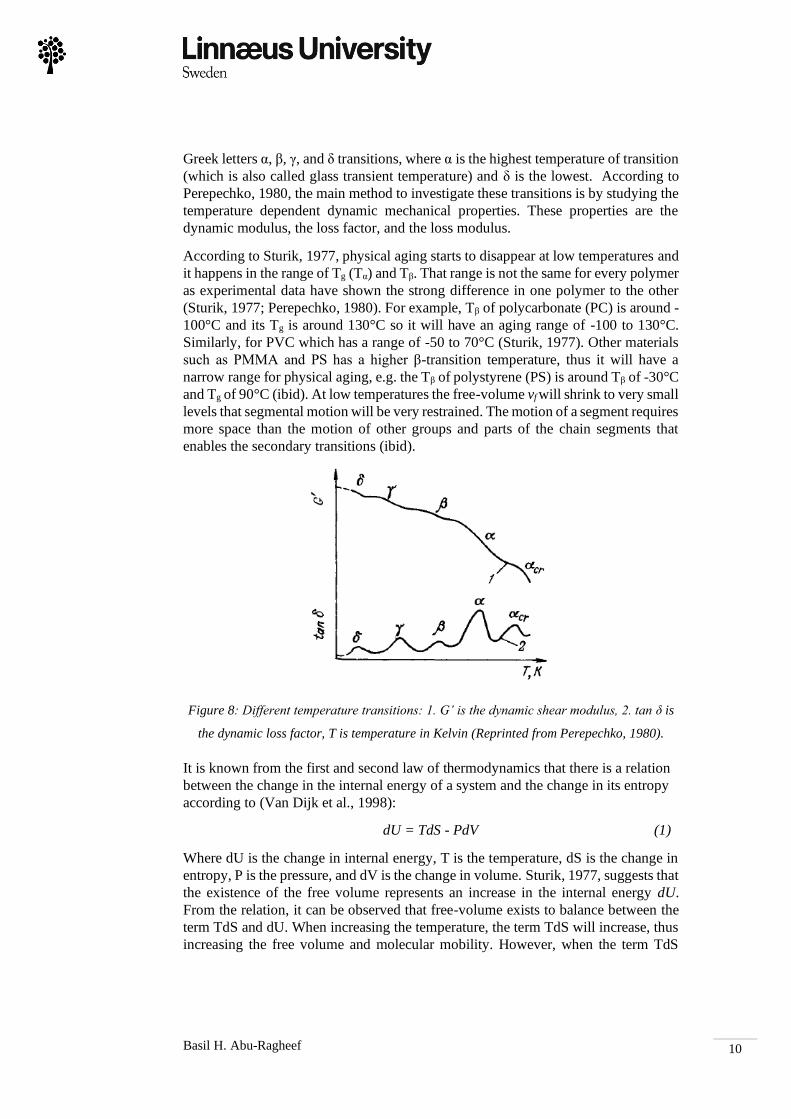
Greek letters α, β, γ, and δ transitions, where α is the highest temperature of transition
(which is also called glass transient temperature) and δ is the lowest. According to
Perepechko, 1980, the main method to investigate these transitions is by studying the
temperature dependent dynamic mechanical properties. These properties are the
dynamic modulus, the loss factor, and the loss modulus.
According to Sturik, 1977, physical aging starts to disappear at low temperatures and
it happens in the range of Tg (Tα) and Tβ. That range is not the same for every polymer
as experimental data have shown the strong difference in one polymer to the other
(Sturik, 1977; Perepechko, 1980). For example, Tβ of polycarbonate (PC) is around -
100°C and its Tg is around 130°C so it will have an aging range of -100 to 130°C.
Similarly, for PVC which has a range of -50 to 70°C (Sturik, 1977). Other materials
such as PMMA and PS has a higher β-transition temperature, thus it will have a
narrow range for physical aging, e.g. the Tβ of polystyrene (PS) is around Tβ of -30°C
and Tg of 90°C (ibid). At low temperatures the free-volume vf will shrink to very small
levels that segmental motion will be very restrained. The motion of a segment requires
more space than the motion of other groups and parts of the chain segments that
enables the secondary transitions (ibid).
Figure 8: Different temperature transitions: 1. G’ is the dynamic shear modulus, 2. tan δ is
the dynamic loss factor, T is temperature in Kelvin (Reprinted from Perepechko, 1980).
It is known from the first and second law of thermodynamics that there is a relation
between the change in the internal energy of a system and the change in its entropy
according to (Van Dijk et al., 1998):
dU = TdS - PdV (1)
Where dU is the change in internal energy, T is the temperature, dS is the change in
entropy, P is the pressure, and dV is the change in volume. Sturik, 1977, suggests that
the existence of the free volume represents an increase in the internal energy dU.
From the relation, it can be observed that free-volume exists to balance between the
term TdS and dU. When increasing the temperature, the term TdS will increase, thus
increasing the free volume and molecular mobility. However, when the term TdS

Basil H. Abu-Ragheef
11
decreases, it will decrease the free volume and molecular mobility consequently
(Sturik, 1977).
In order to understand aging and glass transition, a closed loop can be identified from
the relations discussed above, where the free-volume vf determine the molecular
mobility, while the molecular mobility M determines the change of the free-volume
over the change of time 𝑑𝑣𝑓
𝑑𝑡 (ibid).
𝑣𝑓 → 𝑀 →
𝑑𝑣𝑓
𝑑𝑡
(2)
When cooling the polymer, the free-volume decreases in a non-linear process called
volume relaxation (Kovacs, 1966; Struik, 1966; as cited in Sturik, 1977). During
volume relaxation, the free-volume vf cannot decrease endlessly below a certain
temperature and it almost stops decreasing at a certain point. This happens because
the molecular mobility becomes too small (ibid). After cooling beyond the glass
transient temperature, the rate of change in the free-volume will be very slow due to
the decrease in thermal activation as the molecular motion is thermally activated
(Litovitz et al., 1965; as cited in Sturik, 1977). The slow change in molecular mobility
and volume-relaxation will consequently change the mechanical properties such as
stiffness, creep, stress relaxation, dynamic moduli and other factors that are dependent
on it (Boyer, 1968; Sturik, 1977; Hutchinson, 1995; Ward et al., 2004; Mullins et al.,
2018).
Heating aged polymers to a glass transition temperature Tg will erase its aging effects
on the mechanical properties (Sturik, 1977). However, as time of aging depends on
temperature, the experiments and the effects of aging can be accelerated by using
time-temperature shifting of viscoelastic properties of the material and the
construction of master curves. The time-dependent polymer data such as creep and
stress relaxation can be shifted using methods such as equivalent temperature-time
and time-temperature superposition (Barbero et al., 2004; Malkin et al., 2012).
Acceleration can occur also by adding a solvent, where the behavior can be predicted
by the concentrations of the solvent, this method is called time-concentration
superposition (Malkin et al., 2012). In other words, physical aging can be defined as
the reversible change of material properties primarily by changing the relaxation
times during a certain period of time and temperature range and that it is strongly
influenced by the thermal history of the polymer (Hutchinson, 1995; Sturik, 1977).

Basil H. Abu-Ragheef
12
2.3 Other Polymer Degradation and Aging Processes Erhard et al., 2006, suggests that the mechanical properties of polymers depend to a
large extent on temperature, time, nature of the applied load, and other environmental
effects such as UV radiation and exposure to chemical substances. Aging mechanisms
in polymers can be classified into the criteria in figure 9.
Figure 9: Degradation types (Fotopoulou et al., 2017).
2.3.1 Thermo-oxidation
According to Wright, 2001, 4% of causes of failure in plastics are due to the physical
and chemical processes that happens at various temperature, also known as thermal
degradation. One of the most serious problems related to the use of plastics at elevated
temperature is oxidation (Maxwell et al., 2005). In general, all polymers contain free
radicals which are uncharged molecules that have been developed in the
polymerization process of the polymer. The oxidation process occurs in plastics by
the reaction of these free radicals with oxygen to form peroxide radicals (Maxwell et
al., 2005; Wright, 2001):
(3)
Further oxidation can also occur by slow reactions, in particular by the peroxide
abstracting hydrogen from the polymer molecules (Wright, 2001). The rate of this
degradation will lead to several changes, notably the change in molecular weight
distribution and mechanical properties such as strain at break and impact strength
(ibid).
The durability and induction time, i.e. the initial stage of a chemical reaction, of the
polymer will depend generally on the physical and chemical structure, the stabilizing
additives, and the state of stress in the polymer (ibid). It is generally observed that the
rate of degradation of plastics increases and the maximum continuous use temperature
(MCUT) decreases when heating a stressed polymer (Terselius et al., 1986; as cited
in Wright, 2001). Internal stresses are not enough to break the bonds between the
molecules in the polymer. However, stresses reduce the activation energy required
for the process. Thus, alongside heat, stresses increase the oxygen diffusion through
volume expansion (Wright, 2001). Studies (Minervino et al., 2013; Sang et al., 2017)
have shown the significant effects of thermo-oxidation aging on the mechanical

Basil H. Abu-Ragheef
13
properties of polymers. These effects can include reduction in impact-strength and an
initial increase in Tg. However, some polymers showed well-preserved retention in
elastic strength because it is, unlike impact strength, more dependent on the core
condition of the material. While thermo-oxidation affects mainly the surface of the
material (Sang et al., 2017).
2.3.2 Photo-oxidation and UV degradation
Around 6% of phenomenological failures in polymers are caused by UV attack
(Wright, 2001). The exposure to sunlight or artificial light with the presence of
oxygen will lead to the process of photo-oxidation. The implications of these
processes involve changes in color, molecular weight, embrittlement, reduced impact
strength, microcracking, and reduced strain at break (Write, 2001; Lampman, 2003).
Embrittlement due to UV relies mainly on the depth and intensity of the surface
degradation. The surface degradation is dependent on if the material is transparent or
opaque to UV radiation. Transparent materials will have a degraded layer on both
sides; while, the opaque will have only on one side.
Figure 10: Transparent vs opaque UV degradation layers (Reprinted from Wright, 2001).
Oxygen start to react rapidly with free radicals on the surface of the polymer by UV
radiation or pure thermal means. Long exposure to UV light can cause mild surface
roughening, mud cracking, and severe surface damage. Weathering can be worsened
in severe winter condition through the formation of ice inside the cracks leading to a
failure (ibid). However, in many cases it doesn’t change the performance of the bulk
material.
The color of plastic can change in the rate of thermal- and photo- oxidation through
its surface temperature. Different colors can generate different surface temperatures
(See table 1) depending on how much it radiates the energy it absorbs (Wright, 2001).
The increase of surface temperature will increase the rate of thermal- and photo-
oxidation that will create oxidation products. These products increase the rate of UV
absorption and therefore starts a chain reaction that speeds up the process (ibid).

Basil H. Abu-Ragheef
14
Color Ambient = 26 °C Ambient = 34 °C
White 33 46
Yellow 38 52
Red 40 55
Red 41 56
Green 43 59
Grey 47 63
Brown 49 65
Brown 50 67
Table 1: Surface temperatures at different colors and ambient (Reprinted from Wright,
2001).
2.3.3 Biodegradation
Micro-organisms such as bacteria, fungi, algae and protozoa can be responsible for
degradation of polymers (Wright, 2001). When the organic material is moisturized,
the micro-organisms will multiply and flourish on the surface leaving a hydrated layer
called biofilm. It contains living and dead cells, metabolic byproducts, and other
mixture of micro-organism. These biofilms depend on several factors such as light
intensity, pH level, temperature, and oxygen. Its thickness can range from 100
microns to several centimeters depends on the conditions it has been into (ibid). These
biofilms can cause harmful effects such as the consumption of plasticizers and other
low molecular weight additives. Additionally, it can cause surface stains, chemical
attack and loss of electrical properties (ibid). Biofilms can consume high molecular
weight polymers through their enzymes that chemically attack the polymer and cause
degenerations. In polyurethane (PUR) it can cause cracking and delamination (ibid).
According to Fotopoulou et al., 2017, the biodegradation process is very slow and
require initiation by environmental factors. Studies have shown that the tensile
strength could be decreased due to biodegradation. It can also cause changes in
elongation which can be either a decrease or increase depending on the type of
material (Yabannavar et al., 1994; Tokiwa et al., 2009).
2.3.4 Wet Environments and Water Absorption
In a test done on pDCPD under heavy duty offshore environment it has been found
that its water diffusion is 8.10-13 m2/s at 25°C. This rate is slow compared to other
polymers such as PP and PU (Le Gac et al., 2013). When immersed in sea water,
pDCPD absorbs water in around 1% of its weight, however, this absorption does not
change the Tg or the Young’s Modulus. The latter is due to the plasticization effect of
the material that is triggered by water (ibid). One of the degradation processes in
polymers when being in contact with water is hydrolysis, where hydrogen ions H+ or
hydroxyl ions OH+ in water triggers the degradation process. Hydrolysis leads to
chain scission and reduction in molecular weight. Thus, it causes a reduction in
toughness and strain at failure (Wright, 2001). Hydrolytic degradation also occurs on
the surface since the surface is where most of the moisture concentrate (Lampman,
2003). The effect of this surface degradation will lead to degradation in the short-term
properties of the polymer e.g. reductions in tensile strength, impact strength, and
toughness (ibid).

Basil H. Abu-Ragheef
15
2.4 Tensile and Plastic Behaviors in Polymers Young’s modulus is dependent on test temperature for amorphous polymers. Close to
Tg where the material is in a viscoelastic state, it starts to fall rapidly until the polymer
becomes in a rubbery state (Mullins et al., 2018). Since the thermosets are cross-
linked, the elastic modulus remains almost constant when the temperature keeps
increasing. Tensile behavior is associated with molecular motions and everything that
have an effect on the molecular motion will make changes on its behavior such as the
molecular structure, molecular weight, cross-linking density, and temperature (Rudin,
1998; Mullins et al., 2018).
Figure 11: Young’s Modulus-Temperature curve for polymers showing difference between
Cross-linked and Linear polymers in the rubbery state (Reprinted from Mullins et al., 2018).
In thermosets, shear yielding is most common. If the material does not exhibit an early
brittle fracture, it can undergo plastic deformations at high strain levels (Mullins et
al., 2018). In glassy polymers, if shear yielding is homogeneously distributed on the
vicinity of a crack. The ductile failure will generally occur with the material gaining
high toughness (ibid). This happens since a high portion of the fracture energy is
absorbed by the plastic deformation. Thus, shear yielding can be a toughening
mechanism in polymers (ibid). There are two simple equations that can predict the
start of yielding; Von-Mises and Tresca (Hertzberg et al., 2012; Mullins et al., 2018).
Von-Mises states that the yield will start when the elastic-shear strain-energy density
reaches a critical value.
(𝜎1 − 𝜎2)2 + (𝜎1 − 𝜎2)
2 + (𝜎1 − 𝜎2)2 = 6𝜏𝑦
2 (4)
While Tresca suggests that the yield will start when the maximum shear stress on any
plane reaches a critical value.
|𝜎1 − 𝜎3| = 2𝜏𝑦 (5)
Von-Mises is generally more preferred in the prediction of yielding as it has better
correlation with empirical data (Hertzberg et al., 2012). However, both models were
developed for metals and it may not be accurate in describing the shear yielding of

Basil H. Abu-Ragheef
16
polymers in certain conditions (Mullins et al., 2018). It suggests that yield stresses in
uniaxial tension will be equal to yield stresses in uniaxial compression. However, for
polymers, the compression yield stresses are usually 15% higher than tensile yield
stresses (Landel et al., 1993; Mullins et al., 2018).
Figure 12: Stress-strain behavior of polystyrene under tension and compression (Reprinted
from Landel et al., 1993).

Basil H. Abu-Ragheef
17
2.5 Fatigue Behavior in Polymers
2.5.1 Thermal Fatigue
When applying cyclic stress on a material it initiates microscopic cracks at internal
areas where there is stress concentration. Polymers tend to fail at much lower stresses
due to fatigue than static loading conditions (Sauer et al., 1980). Early studies of
fatigue in polymers have been using unnotched specimen, where it has proved useful
in metals. However, in polymers it might raise the question of heating that can lead
to failure by thermal melting. There is a critical frequency of cyclic loading where
thermal effects need to be considered (Sauer et al., 1980; Ward et al., 2004; Hertzberg
et al., 2012). The viscoelasticity of polymers and its poor conductivity of heat makes
them more sensitive to temperature than metals to the frequency of alternating loads
(Sauer et al., 1980). If isothermal conditions are not met under the loading, hysteretic
energy generated during each cycle will be dissipated as heat and it will rise up the
temperature of the specimen. This makes it more vulnerable to failure from thermal
rapture and melting (Sauer et al., 1980; Hertzberg et al., 2012). The energy lost during
the cyclic loading for a given cycle can be given by the following relation (Ferry et
al., 1970; as cited in Sauer et al., 1980; Hertzberg et al., 2012):
�̇� = 𝜋𝑓𝐽"(𝑓, 𝑇, 𝜎)𝜎2 (6)
Where f is the frequency, J” is the loss compliance, and σ is the stress. By neglecting
heat lost to environment, ∆�̇� will increase with the increase of frequency, stress
amplitude, and internal friction (Sauer et al., 1980; Hertzberg et al., 2012). The
temperature rise will be retrieved through the following relation (Hertzberg et al.,
2012):
∆�̇� =
𝜋𝑓𝐽"(𝑓, 𝑇)𝜎2
𝜌𝑐𝑝
(7)
Where ∆�̇� is the rate of change of temperature over time, 𝜌 is the density, and Cp is
the specific heat. Many examples of temperature rise in fatigue testing of polymers
have been documented. The temperature shows a linear increase with the increase of
frequency in unnotched polyethylene (PE) specimens, that increase becomes rapid
when increasing the applied alternating stress (Sauer et al., 1977; as cited in Sauer et
al., 1980). As for polymethylmethacrylate (PMMA) specimen tested in cyclic
bending at 50 Hz the temperature reached values close to 100 C at failure (Oldyrev et
al., 1975: as cited in Sauer et al., 1980).

Basil H. Abu-Ragheef
18
Figure 13: PE specimen temperature-test speed at different stresses (Reprinted from Sauer
et al., 1977; as cited in Sauer et al., 1980)
Another interesting observation on the influence of stress amplitude on temperature
rise under cyclic load has been observed for polyoxymethylene (POM). For samples
tested at constant testing speed, at 22.4 MPa, the temperature rise steadily until
reaching thermal failure. However, on stresses below 21.6 MPa the temperature will
rise slowly and then stabilizes at the final value (Crawford et al., 1975; as cited in
Sauer et al., 1980). This means that one cannot measure the correct stress/cycle values
at the exact room temperature as the internal temperature of the specimen will keep
rising and is dependent on frequency, stress amplitude, and other material
characteristics (Sauer et al., 1980). When the temperature increases, Young’s
Modulus decreases, thus increasing the deflections, these deflections produce even
more energy that will dissipate as heat with each cycle (Hertzberg et al., 2012).

Basil H. Abu-Ragheef
19
Figure 14: Temperature-cycle rise for POM at different stresses (Reprinted from Crawford
et al., 1975; as cited in Sauer et al., 1980).
In unnotched specimens, temperature increase can be reduced by strain cycling at
constant strain rate instead of stress cycling. As in strain cycling there will be lower
energy dissipation and no thermal discharge, while in stress cycling it is vise-versa.
Unless frequency and stress are kept at lower levels, thermal discharge will occur due
to viscoelasticity (ibid). Testing with unnotched specimens does not distinguish
between crack initiation and crack propagation when studying the fatigue behavior
(Ward et al., 2004). An initial sharp crack can be introduced in order to examine how
the crack propagates using fracture mechanics concept (ibid). Hertzberg et al., 2012
concluded that thermal failure comes in the last stages of cyclic life. To prove this a
number of experiments have been conducted involved introducing periodic resting
times during testing. This method has improved life of the specimen greatly through
cooling down temperatures arise from adiabatic heating (ibid). Other methods
represented by Hertzberg et al., 2012 to suppress thermal fatigue are limiting stress,
decreasing frequency, and increasing the specimen’s surface-to-volume ratio.
2.5.2 Mechanical Fatigue
Test frequency has an influence on the testing process; however, it depends on the
viscoelasticity of the polymer in the test temperature (ibid). In materials where
thermal effects are not dominant, increasing frequency rates might increase fatigue
lifetime. This is due to higher strain rates and tensile modulus. Other reason for the
increase is the generation of localized heat at the crack end. This heat has the ability
to slow down the crack propagation rate. This has been noticed in PS and PMMA
where the crack propagation rate has been decreased with the increase of frequency
i.e. local heat will increase correspondingly (ibid). However, other materials such as
Nylon, PC, and PSF experiments showed no frequency sensitivity (Hertzberg et al,

Basil H. Abu-Ragheef
20
1975; as cited in Sauer et al., 1980). The stress value at which thermal runaway occurs
also depends on the frequency level, In POM it has been found that when lowering
the frequency, the thermal runaway starts at higher stress levels. (Crawford et al.,
1975 as cited in Sauer et al., 1980).
In cyclic loading, fatigue life decreases with the increase of the mean stress. The
change in mean stress also make changes in the fracture surface shape (Sauer et al.,
1980). It has been noticed in some materials such as polystyrene (PS), fatigue
resistance increases if the mean stress is increased while maintaining a constant
maximum stress value (Mukherjee et al., 1971; as cited in Sauer et al., 1980). In purely
tensile cycling mode, concentric growth bands are observed in the fracture of many
polymers such as PS, PE, and PVC (Sauer et al., 1980). The number of cycles/bands
is a function of the stress intensity factor range ∆𝐾. At high values of ∆𝐾 the crack
jumps incrementally at each cycle due to fatigue striations (ibid). Polymer structure
also plays a role in its fatigue life. Crystalline polymers have higher fatigue resistance
than amorphous polymers due to its two-phase structure and its ability to absorb
fracture energy (ibid). Fatigue in crystalline polymers is preceded by formation of a
damage zone at the crack tip, but in glassy amorphous polymers it is preceded by
crazing (ibid). It has been also noticed that the degree of cross-linking has a positive
effect on crack propagation rates and toughness, hence increasing crosslinking
decreased crack propagation rates. This is due to increase in molecular weight and
increased capacity for plastic deformation (ibid).
Basil H. Abu-Ragheef
21
3 Theory
3.1 Linear Elasticity and Stress-Strain Relations Stress and strain are classically defined by the scope of small deformations. The
relationships of each point fixed on the material body will be assumed linear
(Bergström, 2015). The stress component can be illustrated as follows:
●
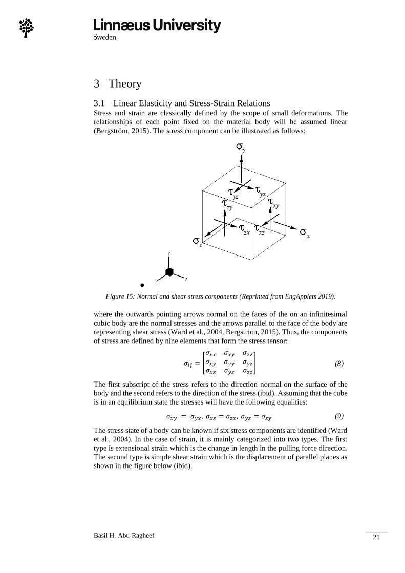
Figure 15: Normal and shear stress components (Reprinted from EngApplets 2019).
where the outwards pointing arrows normal on the faces of the on an infinitesimal
cubic body are the normal stresses and the arrows parallel to the face of the body are
representing shear stress (Ward et al., 2004, Bergström, 2015). Thus, the components
of stress are defined by nine elements that form the stress tensor:
𝜎𝑖𝑗 = [
𝜎𝑥𝑥 𝜎𝑥𝑦 𝜎𝑥𝑧
𝜎𝑥𝑦 𝜎𝑦𝑦 𝜎𝑦𝑧
𝜎𝑥𝑧 𝜎𝑦𝑧 𝜎𝑧𝑧
]
(8)
The first subscript of the stress refers to the direction normal on the surface of the
body and the second refers to the direction of the stress (ibid). Assuming that the cube
is in an equilibrium state the stresses will have the following equalities:
𝜎𝑥𝑦 = 𝜎𝑦𝑥 , 𝜎𝑥𝑧 = 𝜎𝑧𝑥 , 𝜎𝑦𝑧 = 𝜎𝑧𝑦 (9)
The stress state of a body can be known if six stress components are identified (Ward
et al., 2004). In the case of strain, it is mainly categorized into two types. The first
type is extensional strain which is the change in length in the pulling force direction.
The second type is simple shear strain which is the displacement of parallel planes as
shown in the figure below (ibid).

Basil H. Abu-Ragheef
22
Figure 16: Representation of extensional strain (left) and simple shear strain (right)
(Reprinted from Ward et al., 2004).
The angle 𝜃 represents the displacement between the two parallel planes divided by
the perpendicular distance between the same planes (ibid). Strain is a unitless variable
and sometimes it is denoted in percentages. Similar to stress, the components of strain
can be given by the strain tensor (ibid):
휀𝑖𝑗 =
[
𝜕𝑢𝑥
𝜕𝑥
1
2(𝜕𝑢𝑦
𝜕𝑥+
𝜕𝑢𝑥
𝜕𝑦)
1
2(𝜕𝑤
𝜕𝑥+
𝜕𝑢𝑥
𝜕𝑧)
1
2(𝜕𝑢𝑦
𝜕𝑥+
𝜕𝑢𝑥
𝜕𝑦)
𝜕𝑢𝑦
𝜕𝑦
1
2(𝜕𝑢𝑦
𝜕𝑧+
𝜕𝑢𝑧
𝜕𝑦)
1
2(𝜕𝑢𝑧
𝜕𝑥+
𝜕𝑢𝑥
𝜕𝑧)
1
2(𝜕𝑢𝑦
𝜕𝑧+
𝜕𝑢𝑧
𝜕𝑦)
𝜕𝑢𝑧
𝜕𝑧 ]
(10)
In the most evident case, it is assumed that stress and engineering strain are linearly
related to each other. Each of the six components of stress are related to six
independent component of strain (ibid), as shown in the expression of generalized
Hooke’s law for both isotropic and anisotropic solids:
𝜎𝑥𝑥 = 𝑎휀𝑥𝑥 + 𝑏휀𝑦𝑦 + 𝑐휀𝑧𝑧 + 𝑑휀𝑥𝑧 . . . 𝑒𝑡𝑐 (11)
For an isotropic material, the stress is proportional to strain and is unaffected by the
direction or orientation of the body (Ward et al., 2004; Bergström, 2015). Considering
one dimension, e.g. strains in the X direction, we have:
𝜎𝑥𝑥 = 𝐸휀𝑥𝑥 (12)
where E is called the Young’s modulus or the modulus of elasticity. These equations
can be developed into the following form for strains in the y and z direction:
휀𝑥𝑥 = −𝑣
𝐸 𝜎𝑥𝑥, 휀𝑧𝑧 =
−𝑣
𝐸 𝜎𝑥𝑥
(13)
Where v is Poisson’s ratio is the relation between the contraction strain 휀𝑦𝑦 to the
extensional strain 휀𝑥𝑥 (ibid). similarly for the other two direction, we can obtain the
following stress-strain relations:

Basil H. Abu-Ragheef
23
휀𝑥𝑥 =
1
𝐸 𝜎𝑥𝑥 −
𝑣
𝐸(𝜎𝑦𝑦 + 𝜎𝑧𝑧)
휀𝑦𝑦 = 1
𝐸 𝜎𝑦𝑦 −
𝑣
𝐸(𝜎𝑥𝑥 + 𝜎𝑧𝑧)
휀𝑧𝑧 = 1
𝐸 𝜎𝑧𝑧 −
𝑣
𝐸(𝜎𝑥𝑥 + 𝜎𝑦𝑦)
휀𝑥𝑧 = 1
𝐺 𝜎𝑥𝑧, 휀𝑦𝑧 =
1
𝐺 𝜎𝑦𝑧, 휀𝑥𝑦 =
1
𝐺 𝜎𝑥𝑦
𝐺 = 𝐸
2(1 + 𝑣)
(14)
(15)
(16)
(17)
(18)
Where G is the shear modulus which is the constant in the relation between shear
stress and its corresponding shear strain.
Young’s Modulus can be influenced by temperature in polymers. The polymer
structure plays a role in determining the modulus as its molecules are constructed with
covalent bonds and the strength of these can differ from one type to another
(Hertzberg et al., 2012). In highly cross-linked rigid thermosets, where Tg tend to be
high, a change in the molecular structure is difficult to accomplish, thus the material
can have a relatively high Young’s modulus (ibid).
To define stress and strain deformations there are multiple approaches. The classical
approach is through uniaxial deformation where a force is acting perpendicularly to
the cross-sectional area of the tested material specimen as shown in figure 17
(Bergström, 2015). The stress and strain will be calculated as follows:
𝜎 =
𝐹
𝐴
휀 = ẟ
𝐿
(19)
(20)
Where 𝜎 is the stress, F is the force, A is the cross-sectional area of the body. 휀 is the
perpendicular strain, ẟ is the displacement, and L is the original length of the body.
In the small strain theory, it is assumed that the changes in dimensions during loading
are so small that they can be represented using linear representation and there is only
one stress and one strain to measure (ibid).

Basil H. Abu-Ragheef
24
Figure 17: Illustration of uniaxial loading
It is important to make a distinction between engineering stress-strain and true stress-
strain. The terms used extensively in engineering practice are defined as follows
(Hertzberg et al., 2012):
𝜎𝑒𝑛𝑔 =
𝐹
𝐴𝑜
휀𝑒𝑛𝑔 = ẟ
𝐿𝑜
(21)
(22)
Where F is the load, 𝐴𝑜is the initial cross-sectional area, ẟ is the displacement, and
𝐿𝑜 is the initial length While true stress and strain can be defined as:
𝜎𝑡𝑟𝑢𝑒 =
𝐹
𝐴𝑖
휀𝑡𝑟𝑢𝑒 = 𝑙𝑛 𝑙𝑓
𝐿𝑜
(23)
(24)
Where 𝐴𝑖 is the instantaneous cross-sectional area and 𝑙𝑓 is the final length.

Basil H. Abu-Ragheef
25
3.2 Cyclic Stresses Cyclic stresses (or fatigue stresses) are common in engineering problems, for
example, alternating stresses accompanying a rotating shaft, pressurizing and
depressurizing cycles of an aircraft, and load fluctuations affecting wings (Hertzberg
et al., 2012). According to Wright, 2001, fatigue is the second most common cause
of failure and account to 15% of failures in plastics. The design engineer must be
aware of the risk of cyclic loads, which are common in vehicles, that might cause
failure to the product (ibid). A general fatigue failure involves initiation of a crack
that keep propagates with each cycle until the material fails and fractures. This
happens within intermediate values of stress that falls between ¼ and ½ of the tensile
or ultimate stress (Sauer et al., 1980). Cracks can be classified into two categories;
small cracks that interacts with the microstructure of the material and are shear driven,
and large cracks that are almost insensitive to the microstructure of the material and
are tension driven (Ekberg, 1998). Small cracks tend to propagate faster than larger
ones. However, crack closure phenomena is asserted in large cracks. It is one of the
causes of crack arrestment where fatigue crack growth rate will be decreased due to
residual stresses (ibid).
Figure 18: Stages of crack initiation and propagation (Reprinted from Ekberg, 1998).
Studies of fatigue fracture in polymers are usually made by fracture mechanics
experiments (ibid). In notched specimens, the stress intensity factor can be calculated
through the following relations:
𝐾 = 𝑌𝜎√𝑎 (25)
Where K is the intensity factor, Y is the geometrical value (√𝜋 for a central crack
length of 2a), and 𝜎 is the stress (ibid). These tests are usually performed with a stress
ratio of 0.1 where R = min stress/max stress (ibid). In order to study the service life
of a material that is going to be used in designing a new part, the integration of the
Paris equation can be used with the start and end of the flaw as integration limits
(Ekberg, 1998; Hertzberg et al., 2012, Ward et al., 2004):
Basil H. Abu-Ragheef
26
𝑑𝑎
𝑑𝑁= 𝐴∆𝐾𝑚
(26)
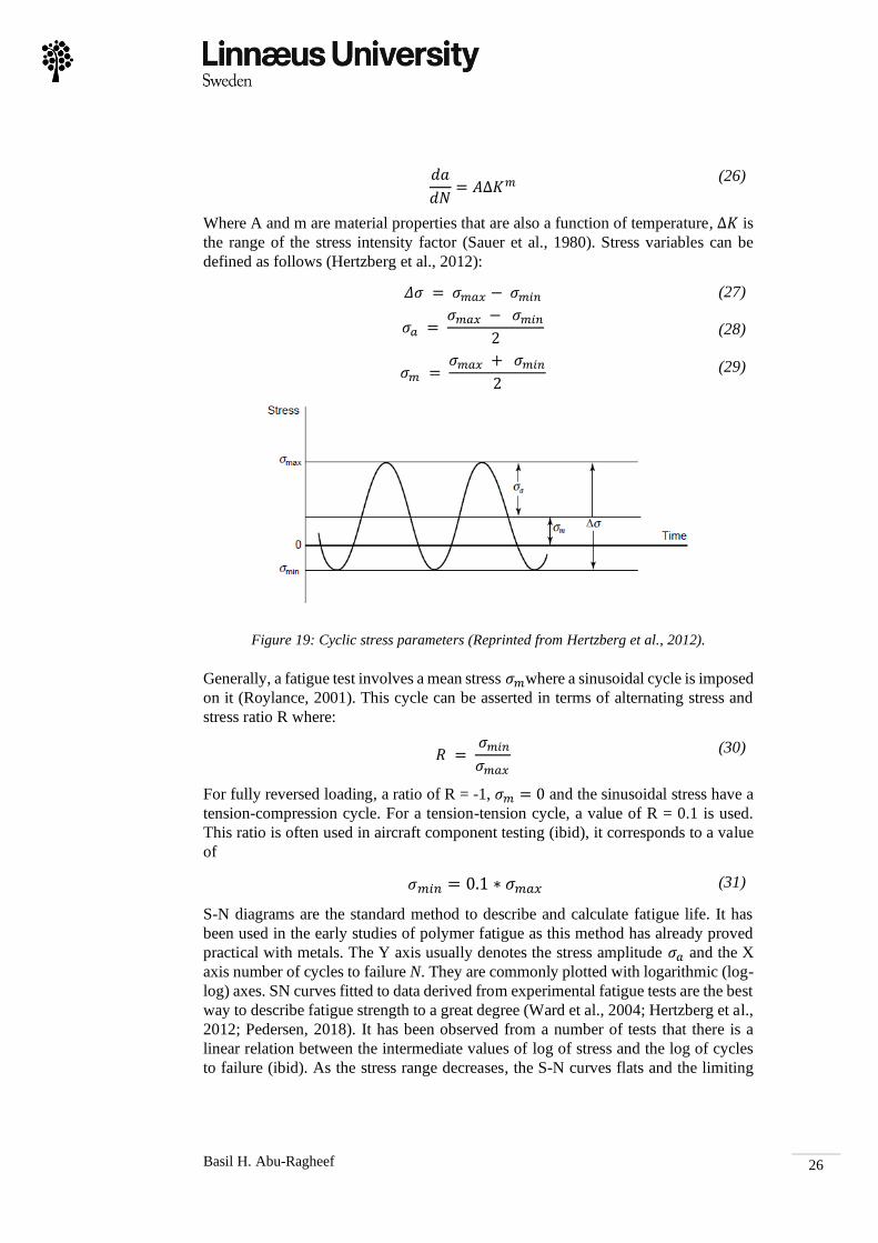
Where A and m are material properties that are also a function of temperature, ∆𝐾 is
the range of the stress intensity factor (Sauer et al., 1980). Stress variables can be
defined as follows (Hertzberg et al., 2012):
𝛥𝜎 = 𝜎𝑚𝑎𝑥 − 𝜎𝑚𝑖𝑛
𝜎𝑎 = 𝜎𝑚𝑎𝑥 − 𝜎𝑚𝑖𝑛
2
𝜎𝑚 = 𝜎𝑚𝑎𝑥 + 𝜎𝑚𝑖𝑛
2
(27)
(28)
(29)
Figure 19: Cyclic stress parameters (Reprinted from Hertzberg et al., 2012).
Generally, a fatigue test involves a mean stress 𝜎𝑚where a sinusoidal cycle is imposed
on it (Roylance, 2001). This cycle can be asserted in terms of alternating stress and
stress ratio R where:
𝑅 = 𝜎𝑚𝑖𝑛
𝜎𝑚𝑎𝑥
(30)
For fully reversed loading, a ratio of R = -1, 𝜎𝑚 = 0 and the sinusoidal stress have a
tension-compression cycle. For a tension-tension cycle, a value of R = 0.1 is used.
This ratio is often used in aircraft component testing (ibid), it corresponds to a value
of
𝜎𝑚𝑖𝑛 = 0.1 ∗ 𝜎𝑚𝑎𝑥 (31)
S-N diagrams are the standard method to describe and calculate fatigue life. It has
been used in the early studies of polymer fatigue as this method has already proved
practical with metals. The Y axis usually denotes the stress amplitude 𝜎𝑎 and the X
axis number of cycles to failure N. They are commonly plotted with logarithmic (log-
log) axes. SN curves fitted to data derived from experimental fatigue tests are the best
way to describe fatigue strength to a great degree (Ward et al., 2004; Hertzberg et al.,
2012; Pedersen, 2018). It has been observed from a number of tests that there is a
linear relation between the intermediate values of log of stress and the log of cycles
to failure (ibid). As the stress range decreases, the S-N curves flats and the limiting

Basil H. Abu-Ragheef
27
stress will be called endurance limit where no fatigue will happen below that stress
(ibid).
Figure 20: Typical S-N curve (Reprinted from Hertzberg et al., 2012).
A major aspect the when conducting tests on polymers to be aware of the influence
of adiabatic heating that can generate when doing fatigue tests in polymers. Meaning
that there will be not enough time for heat to dissipate thus increasing the temperature
of the polymer that can lead to thermal fatigue (Sauer et al., 1980; Ward et al., 2004;
Hertzberg et al., 2012).

Basil H. Abu-Ragheef
28
3.3 Viscoelastic Behavior of Polymers There are two constitutive models that can describe the mechanical properties of ideal
materials (Ottosen et al., 2005; Malkin et al., 2012):
1. Newton’s law of Liquids:
𝜎𝑣 = 𝜂휀̇𝑣 (32)
2. Hooke’s law of Solids:
𝜎𝑒 = 𝐸휀𝑒 (33)
Where in the first law 휀𝑒 is rate of change in shear strain, 𝜎𝑣 is the shear stress, and
η is the viscosity. In the second law ε is the strain, 𝜎𝑒 is the tensile stress, and E is the
Young’s modulus. Polymers have an interesting feature where it shows both
behaviors and act as an elastic solid or a viscous liquid depending on temperature and
experiment time, this kind of behavior is called viscoelasticity (Ward et al., 2004).
Newton’s law of viscosity can be translated to the following equation (ibid):
𝜎 = 𝜂
𝜕𝑉𝑥𝜕𝑦
(33)
Where 𝑉𝑥 is the velocity and y is the direction of the velocity gradient. Since velocity
is the change of displacement with time, in an xy-plane we get the following equation
(ibid):
𝜎𝑥𝑦 = 𝜂 [
𝜕
𝜕𝑦(𝜕𝑢𝑥
𝜕𝑡) +
𝜕
𝜕𝑥(𝜕𝑢𝑦
𝜕𝑡)] = 𝜂
𝜕
𝜕𝑡(𝜕𝑢𝑥
𝜕𝑦+
𝜕𝑢𝑦
𝜕𝑥)
(34)
Where 𝑢𝑥 and 𝑢𝑦 are the displacement in x and y directions respectively, and t is time.
It can also be written as (ibid):
𝜎𝑥𝑦 = 𝜂
𝜕휀𝑥𝑦
𝜕𝑡
(35)
Where 휀𝑥𝑦 is the shear strain. In Hooke’s law the stress is linearly related to the strain,
however, in the above equation it is linearly related to the change in strain over time
(ibid). For the elastic behavior the shear modulus will be used instead of the elastic
modulus in order to build a simple constitutive relation for the viscoelastic behavior.
The simplest possible form of linear viscoelasticity is (ibid):
𝜎𝑥𝑦 = (𝜎𝑥𝑦)𝐸 + (𝜎𝑥𝑦)𝑉 = 𝐺ε𝑥𝑦 + 𝜂
𝜕ε𝑥𝑦
𝜕𝑡
(36)
This formulation is called the Kelvin-Voigt model. However, there are multiple
possible formulation of viscoelastic behavior to unite those constitutive relations
(ibid). For better understanding these relations, it can be illustrated by simple
mechanical models. Viscous behavior is modeled as a dashpot (damper) and the
elastic behavior is modeled after a spring (Bergström, 2015; Malkin et al., 2012; Ward
et al., 2004). The use of these models is very instructive and it increases our capacity
to understand material behavior in different stress-strain conditions (Malkin et al.,
2012).

Basil H. Abu-Ragheef
29
Figure 21: The fundamental mechanical models representing viscoelasticity, on the top is
the Kelvin-Voigt model and on the bottom is the Maxwell model.
As illustrated in figure 21, the Kelvin-Voigt model consists of a spring with a spring
modulus E in parallel with a dashpot with viscosity 𝜂. If constant stress is applied, the
spring do not deform instantly as it is going to be retarded by the dashpot as the stress
is shared by both components in the parallel connection. After a period of time
dependent on the viscosity 𝜂, the spring will be fully deformed. However, when
removing the stress, the process will be reversed and it will return to its initial
unstretched state (Ward et al., 2004). The Maxwell model represent a spring and a
dashpot series connection. When applying constant displacement, it will immediately
deform the spring. As time proceeds, the deformation will be transferred to the
dashpot element and the spring will be released (Malkin et al., 2012; Ward et al.,
2004). Both Maxwell and Kelvin-Voigt models predict the behavior of different
materials as Maxwell is suited for liquids and Kelvin-Voigt for solids. These models
can be combined in parallel and in series together to predict behavior such as the
Zener model or Burgers model which is a quantitative model of behavior of polymers
(Malkin et al., 2012; Ottosen et al., 2005; Moczo et al., 2006). In general, the series
connection makes the stress equal and strain additive, while the parallel connection
makes the strain equal and the stress additive. From these rules mathematical
formulations can be drawn for different models (Moczo et al., 2006).
Viscoelastic processes can be determined from simple creep and stress relaxation
experiments. Creep is the time-dependent deformation that occurs while applying a
constant stress. On the contrary, stress relaxation is the time-dependent change in
stress when applying a constant strain (Ward et al., 2004). Wright, 2001, suggests that
8% of failures in polymers are due to creep or stress relaxation behaviors. This is due
to a number of reasons including delayed buckling or decline in mechanical jointing
forces. Poor design decisions can also lead to creep/stress relaxation failures. Data
related to such behavior are limited or not sufficient for the design engineer to make
proper design decisions. Creep and relaxation behavior are also heavily dependent on
the temperature. The design engineer needs to be informed about how temperature
change influences the viscoelastic behaviors (ibid). The Kelvin-Voigt model is more
suitable for modeling the creep behavior as first approximation. While the Maxwell
model has more value in modeling a stress relaxation behavior to a first approximation
(Ward et al., 2004).

Basil H. Abu-Ragheef
30
Figure 22: Time dependent behavior of (a) stress-relaxation, (b) creep (Reprinted from
Ashter, 2013).
One of the simplest and most used ways to express the viscoelastic behavior of
polymers is through linear viscoelasticity. A fundamental rule in linear viscoelasticity
is to consider “Each loading step makes an independent contribution to the final
state.” which can also be called Boltzmann superposition (Bergström, 2015). Thus,
strain history will be considered as a sum of infinitesimal strains:
휀(𝑡) = ∑ ∆휀𝑖𝐻(𝑡 − 𝜏𝑖)
∞
𝑖=1
(37)
When applying this to stress we obtain the stress response:
𝜎(𝑡) = ∑ ∆휀𝑖𝐸𝑅(𝑡 − 𝜏𝑖)
∞
𝑖=1
(38)
In cyclic loading, e.g. sinusoidal strain, there will be a lag between applied strain and
stress response. The stress response is also sinusoidal but is shifted with a phase angle
δ (ibid). In case of applying a sinusoidal strain:
휀(𝑡) = 휀𝑚 + 휀𝑎sin (𝜔𝑡) (39)
Where, 휀𝑚 is the mean strain, 휀𝑎 is the strain amplitude and ω is the angular
frequency. The following stress response is obtained:
𝜎(𝑡) = 𝜎𝑚 + 𝜎𝑎sin (𝜔𝑡 + 𝛿) (40)
This can be re written in terms of phase difference with the applied strain (ibid):
𝜎(𝑡) = 𝜎𝑚 + 𝜎𝑎 cos(𝛿) sin(𝜔𝑡) + 𝜎𝑎 sin(𝛿) cos(𝜔𝑡) (41)
Let us define the storage modulus E’ and loss modulus E”. E’ represents the elastic
response that represents the energy stored in the specimen and is in phase with the

Basil H. Abu-Ragheef
31
strain, while E” is the viscous response that represents the energy dissipated out of
the specimen and is lagging 90o from the strain. The latter is also connected to the
heat dissipation during cyclic loading (Ward et al., 2004, Bergström, 2015). The stress
response can be given by:
𝜎(𝑡) ≡ 𝜎𝑚 + 휀𝑎𝐸′sin(𝜔𝑡) + 휀𝑎𝐸" cos(𝜔𝑡) (42)
By defining a complex modulus E* we can get the following relations:
𝐸′ = 𝐸∗cos (𝛿)
𝐸" = 𝐸∗sin (𝛿)
(43)
(44)
Given (Bergström, 2015):
𝐸∗ =𝜎𝑎
𝜀𝑎 (45)
The complex modulus is also treated as a complex number, hence the name, as shown
in the relation:
𝐸 ∗ = 𝐸’ + 𝑖𝐸” (46)
Where i is the imaginary unit (Lakes, 2019, Bergström, 2015). The ratio between the
loss to storage modulus is called the damping ratio, it is given as:
tan 𝛿 =
𝐸"
𝐸′
(47)
Thus, when the damping ratio increase, the material tends to dissipate energy, while
if it decreases, it tends to store the energy and becomes closer to a purely elastic
material (Menard et al., 2006). The phase difference δ can be calculated through the
following relation:
𝛿 = (
2𝜋 𝛥𝑡
T)
(48)
Where T is the time needed for one cycle of load. Δt is the time difference between
the stress and strain curves (Lakes, 2019).

Basil H. Abu-Ragheef
32
Figure 23: Sinusoidal wave of normalized stress and strain (Reprinted from Lakes, 2019).

Basil H. Abu-Ragheef
33
4 Methods
This study will be carried out using a mix of qualitative and quantitative approaches.
The data gathered from the tests are analyzed by statistical models, i.e. this approach
will be qualitative. However, an investigation of the failed specimens will be carried
out using a microscope. This observation method is qualitative and its results will be
correlated with the quantitative results in the final analysis.
4.1 Determination of Tensile Properties
4.1.1 Uniaxial Tension Testing
In order to determine the tensile properties of the plastic material the methods and
guidelines specified in ISO 527-1:2018 have been used. It is used to investigate the
tensile properties of specimens such as the relationship between stress and strain,
tensile strength, and Young’s Modulus (ISO 527-1:2018). These guidelines are
suitable for rigid thermosets including filled and reinforced composites (ibid). A dog-
bone shaped specimen is used for uniaxial tensile tests. This specimen design is
adequate for creating a uniform uniaxial deformation and stress state in the gauge of
the specimen. It also reduces the stress concentrations in the parts that are close to the
grips of the testing machine (Bergström, 2015). The guidelines for the design of test
specimens for plastic materials defined at ISO 20753:2018. One drawback of the dog-
bone shape of test specimens is the necking phenomena. It creates an inhomogeneous
deformation in the specimen which makes it difficult to measure the actual stress-
strain response (Bergström, 2015). One way to solve this issue is through using a
digital image correlation (DIC) system (ibid). The results of this test can be plotted as
a stress-strain plot, the elastic modulus can be calculated by finding the slope of the
flat elastic region (McKeen, 2016) as shown in figure 24 below:
Figure 24: Stress-Strain curves and Necking phenomena in dog-bone shaped specimen
(Reprinted from: ADMET, 2019)

Basil H. Abu-Ragheef
34
4.1.2 Creep Testing
Creep testing guidelines ISO 899-1:2017 shall be followed. Creep is carried out by
applying constant load on a specimen for a certain period of time while monitoring
the change in its strain levels. It can be sensitive to the geometry and service history
of the tested material during testing. For precise results it is desirable that the testing
is done over a broad range of stresses, times, and ambient conditions (ibid). The
specimens are to be loaded smoothly with the desired load being reached in 1-5
seconds. The results shall be later presented in creep curves showing strain against
time and creep modulus against time (ibid).
4.1.3 Digital Image Correlation (DIC)
Digital image correlation is an image processing method that uses recorded images to
capture and analyses measurement data (Schreier et al., 2009). This method is applied
to acquire high resolution strain data by recording images of a loaded, patterned
specimen. A speckle pattern is suitable for DIC strain measurements where the DIC
system can locate the random dots and capture its deformation behavior (Cintrón et
al., 2008). The DIC measurements are dependent on a number of variables which are
the image resolution, pixels, the geometry of the specimen, focal length of the camera,
distance between the recorded specimen and the camera, and the speckle pattern
applied on the specimen (ibid). DIC measurements are similar to those obtained from
direct strain gauges attached to the tested specimen. However, it provides advantages
in terms of relative ease, less preparation times and data analysis (Hensley et al.,
2017). For this research, GOM ARAMIS DIC system has been used to measure
strains during tensile tests. The system is equipped with two 75mm lens cameras and
has been calibrated according to the test settings. Later the data was analyzed using
GOM Correlate 2018 software.

Basil H. Abu-Ragheef
35
4.2 Mechanical and Thermal Fatigue
4.2.1 Cyclic Tension Test
The guidelines specified in the standard ASTM D7791 − 17 covers the determination
of dynamic fatigue properties of plastics in uniaxial loading conditions. Tension or
compression loading can be used in order to determine these properties. For tension
loading condition, a specimen of a rectangular cross-section is gripped by its ends and
pulled in opposite directions equally then released back to its initial condition (ASTM
D7791 − 17). The load will be cyclic and at least four stress levels will be tested. The
test frequency is uniform and it ranges from 1-25 Hz. After fracture it can be
determined at which number of cycles the specimen has failed. For fatigue analysis,
a cyclic stress level shall be applied and a S-N curve will be constructed denoting the
stress level versus the number of cycles to failure.
4.2.2 Thermography
A high-performance IR camera (FLIR A65) is used to capture thermal activity in the
specimen during cyclic loading testing. The camera has a focal length of 13 mm and
IR resolution of 640x512 pixels with a spectral range of 7.5–13 µm. A software is
included to capture the data out of the camera and record it into a picture, video, or
spreadsheet format. Thermography is capable of opening a wide range of application
in thermomechanical processes such as mechanical damages and phase
transformations of materials and its inner structural state. The rate of temperature
increase at crack tips during fatigue can be a good indicator to predict the final failure
state (Yang et al., 2004).

Basil H. Abu-Ragheef
36
4.3 Statistical Approaches
4.3.1 Regression Analysis
Regression analysis is a method used to identify relationships between two sets
measured data (Draper et al., 2014; as cited in Maurer, 2017). It is a method used in
understanding how variables affect one another by predicting the change in one
variable given that another variable has changed. Knowing this relationship enables
predictions e.g. the prediction of the fatigue life of a product under a certain cyclic
load amplitude. However, those relationships are not exact and they need a random
component in the equation that relates the variables. This random component can take
into account unknown factors that are not measured in the data (Walpole et al., 2017).
The fitted line regression line equation is given by:
�̂� = 𝑏𝑜 + 𝑏1𝑥 (49)
Where �̂� is the predicted value, 𝑏𝑜, 𝑏1 are estimates to the parameters β0 and β1
correspondingly, which are unknown intercept and slope parameters (ibid). b0, b1 can
be found through the following equations:
𝑏𝑜 = �̅� + 𝑏𝑜�̅� (50)
𝑏1 = 𝑟
𝑆𝑦
𝑆𝑥
(51)
Where �̅� is the y sample mean, �̅� is the x sample mean, 𝑆𝑦, and 𝑆𝑥 are the standard
deviations of the samples y, x correspondingly, r is the correlation between x and y.
A common regression method is Least Squares. It is important to understand the
concept of residual in the least square’s method. It is considered as an error in the fit,
which will lead to the following relationship (ibid):
𝑦 𝑖 = 𝑏𝑜 + 𝑏1𝑥 + 𝑒𝑖 (52)
The least square method is about finding the values of 𝑏𝑜 and 𝑏1where the sum of the
squares of the residuals 𝑒𝑖 is at its minimum (ibid). The least square estimates can be
computed from the following formulas:
𝑏1 =
𝑛∑ 𝑥𝑖𝑦𝑖𝑛𝑖=1 − (∑ 𝑥𝑖
𝑛𝑖=1 )(∑ 𝑦𝑖
𝑛𝑖=1 )
𝑛 ∑ 𝑥𝑖2𝑛
𝑖=1 − (∑ 𝑥𝑖𝑛𝑖=1 )
2 =∑ (𝑥𝑖 − �̅�)𝑛
𝑖=1 (𝑦𝑖 − �̅�)
𝑛∑ (𝑥𝑖 − �̅�)2𝑛𝑖=1
(53)
𝑏𝑜 =
∑ 𝑦𝑖 − 𝑏1 ∑ 𝑥𝑖𝑛𝑖=1
𝑛𝑖=1
𝑛= �̅� − 𝑏1�̅�
(54)
The coefficient of determination or R2 is used to determine how the regression line
fits the data and it is a value range between 0 and 1 (ibid). R2 is calculated from:
𝑅2 =
𝑆𝑆𝑅
𝑆𝑆𝑇=
∑ (�̂�𝑖 − �̅�)2𝑛𝑖=1
∑ (𝑦𝑖 − �̅�)2𝑛𝑖=1
= 1 −𝑆𝑆𝐸
𝑆𝑆𝑇
(55)
Where SST is total corrected sum of squares, SSE is the variation due to error, and
SSR is the regression sum of squares. However, linear regression does not fit all data

Basil H. Abu-Ragheef
37
sets. Other methods can be used for different data sets such as polynomial regression
and other non-linear fitting (Wu, 2019).
4.3.2 Bootstrap Confidence Intervals
Bootstrapping is an approach to statistical inference that increases sample size by
creating a new sample distribution through resampling given data (Fox, 2002). This
method is most feasible with modern computing power due to its need of performing
computations on the data itself. As (Efron, 1979; as cited in Fox, 2002) has
mentioned, the name “Bootstrapping” is coming from the expression “Pull oneself up
by one's bootstraps” meaning that the data is increasing through its own means.
Resampling gives an approximation of how the point estimate may vary. The newly
generated samples would be used to construct a confidence interval of a given
percentage (Orloff et al., 2014). Confidence intervals are defined as an approach in
statistical inference used to estimate a range of values in which it is probable that it
will include a wanted population parameter. This range of values is calculated from a
set of the sample data, and is dependent on the sample mean (Walpole et al., 2017).
This method is used in a computer program to determine a measure of accuracy
through confidence intervals in the regression lines of fatigue data.

Basil H. Abu-Ragheef
38
4.4 Failure Analysis through Visual Examination Visual analysis is an important approach to investigation of failures (Shah, 2007).
Analyzing material failure require the identification of crack mechanisms that has
been developed. Usually, cracks leave a series of traces and markings that can help in
identifying the direction and motion of the crack. Stress level, crack growth direction,
and the loading conditions are all valuable to understand the failure (Hertzberg et al.,
2012). In polymers, plastic deformation capacity differs from one type to another.
Therefore, the visible evidence is valuable in evaluating fracture in polymers. Crazes
and shear bands can indicate the presence of damage accumulation, concentrated
yielding, and energy absorption before fracture (ibid). It is commonly categorized that
brittle polymer fracture has low strain at failure, i.e. less than 4%. Furthermore,
failures with greater strain are considered ductile (ibid). A digital microscope is used
to investigate the fracture of the tested specimen in order to identify the reasons for
early failures.
Figure 25: Possible reasons for a number of visible defects (Shah, 2007).

Basil H. Abu-Ragheef
39
4.5 Experimental Implementation
4.5.1 Specimens Preparation
Five sheets cut directly from vehicles have been provided by Volvo CE in order to
conduct this research (See appendix 1). 75 Specimens have been cut from the sheets,
15 from each sheet. The sheets and specimens were cut using waterjet to prevent any
unwanted heat that may arise from conventional machining processes. The design of
the specimens have been done using the CAD software SolidWorks. The dimensions
have been derived from A2 Specimen in ISO 20753:2018 standard for plastic testing
specimens except for the gauge length and thickness. The reason was due to variable
thicknesses and curvatures in the sheets due to the design of the vehicle cabin that the
sheets were cut from. Curvature could translate to curves in longer specimens and
changing the thickness will damage the surface and thus will affect the actual fatigue
performance (Pedersen, 2018; Bayoumi et al., 1995).
Figure 26: Dog-bone specimen dimension and tolerances used in the forthcoming tests
(Dimensions are in millimeters).
An investigation has been conducted to ensure that the new gauge length will have
same stress results as the standard length using the finite element method (FEM)
software SIMULIA™ Abaqus. The finite element method is a numerical approach
that solves differential equations which describe a physical problem (Ottosen et al.,
1992). The boundary conditions entered to the program simulated a uniaxial tensile
test. One end of the specimen was fixed by making the displacement in the X-
direction as well as rotations around Y- and Z- axis equals 0. A force of 1500 N was
applied in the opposite end of the specimen towards the X-direction. The material
model used is pure elastic with a Young Modulus of 660 MPa and a Poisson's ratio
of 0.39. The results showed similarities when simulating both lengths on the same
stress level where both specimens experienced a stress level of 37.5 MPa in the middle
of the gauge. The simulation results are shown in the figure below:

Basil H. Abu-Ragheef
40
Figure 27: FEM simulation of the (1) A2 Specimen specified in ISO 20753:2018 and (2) The
modified specimen with 30mm gauge length
After cutting, the specimens were categorized into groups according to its age, color,
and test type. The names given to the specimens were containing the letters of the age
group, test type, color, specimen number, and date of testing, for example
A_S_Y_1_20190506 and C_S_BK_5_20190506. The following table was made to
make a relation between each acronym that has been used in the naming of the
specimens:
Age Group Acronyms Test Type Acronyms Color Acronyms
Virgin A Tensile S Black BK
2013 B Fatigue F Yellow Y
2012 C Creep C
2002 D
Table 2: Acronyms of the specimens naming
4.5.2 Testing Setup
The test and data acquisition have been conducted using an MTS 810 servo-
hydraulic material testing machine. In order to avoid inaccuracies generated
from the original loadcell behind the hydraulic grips in the test machine, a load
cell has been put closer to the grips as shown in the figure below.
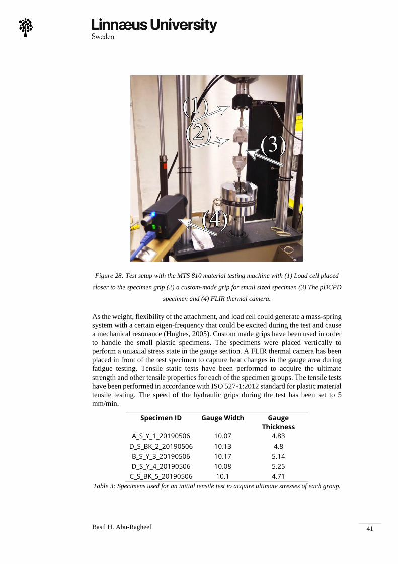
Basil H. Abu-Ragheef
41
Figure 28: Test setup with the MTS 810 material testing machine with (1) Load cell placed
closer to the specimen grip (2) a custom-made grip for small sized specimen (3) The pDCPD
specimen and (4) FLIR thermal camera.
As the weight, flexibility of the attachment, and load cell could generate a mass-spring
system with a certain eigen-frequency that could be excited during the test and cause
a mechanical resonance (Hughes, 2005). Custom made grips have been used in order
to handle the small plastic specimens. The specimens were placed vertically to
perform a uniaxial stress state in the gauge section. A FLIR thermal camera has been
placed in front of the test specimen to capture heat changes in the gauge area during
fatigue testing. Tensile static tests have been performed to acquire the ultimate
strength and other tensile properties for each of the specimen groups. The tensile tests
have been performed in accordance with ISO 527-1:2012 standard for plastic material
tensile testing. The speed of the hydraulic grips during the test has been set to 5
mm/min.
Specimen ID Gauge Width Gauge
Thickness
A_S_Y_1_20190506 10.07 4.83
D_S_BK_2_20190506 10.13 4.8
B_S_Y_3_20190506 10.17 5.14
D_S_Y_4_20190506 10.08 5.25
C_S_BK_5_20190506 10.1 4.71
Table 3: Specimens used for an initial tensile test to acquire ultimate stresses of each group.

Basil H. Abu-Ragheef
42
Fatigue testing has followed the standard ASTM D7791 − 17 for plastic fatigue tests.
All specimens have been assigned a special ID name and its width and thickness
measured before testing (see Appendix 2). Each Fatigue test specimens have been
grouped depending on its stress level. The first stress level was calculated from 0.75
or 0.66 from the ultimate force acquired from the tensile tests. This ratio was chosen
based on the assumption that this force will keep the fatigue failure beyond the low-
cycle fatigue as this research interest is in the high-cycle region where N to failure is
> 103 - 104 cycles (Affonso, 2006). Other stress levels are chosen during the test and
number of cycles to failure. Each group has been tested on 4 different load levels and
each test has been repeated 3 times. The stress was lowered for each level during the
test depending on the number of cycles each level has been failed at. Due to the
limitations in time and the large number of specimens, the tests were stopped after
crossing 120,000 cycles. The specimens which cross the life of 120,000 cycles would
be considered as survivors. The stress ratio of this test R = 0.1 i.e.:
σmin = 0.1 * σmax (56)
Pre-stressing was applied by applying a load equals to the mean of the minimum and
maximum force before applying the cyclic load. All the force levels used, mean, and
amplitude can be found in Appendix 2. It is important to note that prestressing can
increase embrittlement in the structure of the polymer (Wright, 2001). The test
frequency chosen was10 Hz for the first 9 specimens. However, it was changed later
to 15 Hz to speed up the testing process. During this change, the thermal activity was
monitored to ensure that the specimens stayed below the critical levels that can affect
the age state of the specimen.
Creep testing followed ISO 899-1:2017 guidelines. Three stress levels were tested by
applying each stress level for 10 minutes. This time was chosen due to the limited
time budget of this research.
To analyze strain data with the digital image correlation (DIC) system. It had to be
calibrated with the test settings used for this research. The GOM ARAMIS DIC
system is provided with calibration panels that are each one has a unique resolution.
The chosen panel was CP20/175x140/D08067 due to its adaptability with the size of
the test specimens. The calibration measuring volume chosen was 165 / 125 / 105 mm
with a working distance of 620mm and a height variance of 64mm, distance of 241
mm and angle of 25.3o between the cameras. The calibration and test capture
processes where handled through a special software provided by GOM. The system
has been connected to the MTS 810 testing machine using an analog interface to
synchronize force signal with the captured strains. The room temperature for all the
tests was 23-24ºC.

Basil H. Abu-Ragheef
43
4.5.3 Data Preparation and Analysis
In order to handle the data from the test machine, some routines have been
programmed using Python programming language. Python is considered as a great
open source tool for data analysis (Python Software Foundation, 2019). Python has
been chosen due to its free and widespread data analysis packages and its relative ease
of use. In cyclic load testing, the data output from the test machine comes in two .dat
files. The first routine was programmed to clean the .dat files coming from the test
and convert them into readable .csv files. The rest of the routines were made to
process data and produce various plots and regression lines. The code can be accessed
in Appendix 5.
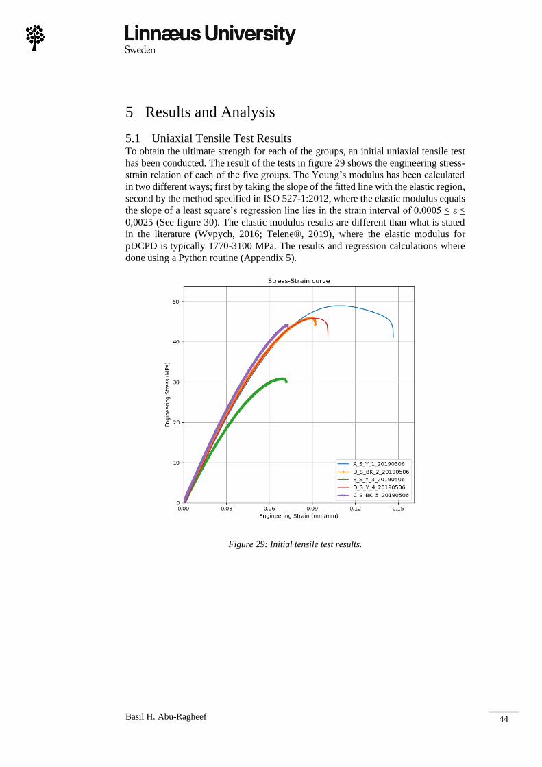
Basil H. Abu-Ragheef
44
5 Results and Analysis
5.1 Uniaxial Tensile Test Results To obtain the ultimate strength for each of the groups, an initial uniaxial tensile test
has been conducted. The result of the tests in figure 29 shows the engineering stress-
strain relation of each of the five groups. The Young’s modulus has been calculated
in two different ways; first by taking the slope of the fitted line with the elastic region,
second by the method specified in ISO 527-1:2012, where the elastic modulus equals
the slope of a least square’s regression line lies in the strain interval of 0.0005 ≤ ε ≤
0,0025 (See figure 30). The elastic modulus results are different than what is stated
in the literature (Wypych, 2016; Telene®, 2019), where the elastic modulus for
pDCPD is typically 1770-3100 MPa. The results and regression calculations where
done using a Python routine (Appendix 5).
Figure 29: Initial tensile test results.

Basil H. Abu-Ragheef
45
Figure 30: Stress-Strain curve for specimen D_S_Y_4_20190506 with the two approaches to
finding the Young’s modulus.
Young’s modulus values have been approximated using the ISO least squares
regression and the yield region slop methods were significantly different as shown in
figure 32. It can be assumed that the inaccuracies in the strain data are coming from
the extensometer. By comparing both Digital Image Correlation (DIC) and
extensometer strains, the DIC supported strain measurement showed significant
differences in terms of strain in contrast with strain data acquired with the test
machine’s extensometer. The difference in stiffness (elastic modulus) between each
group can also be seen more clearly in the DIC data plot as shown in figures 33 and
34. To calculating the modulus in both the DIC and the extensometer, the least
square’s regression line strain interval has been modified from 0.0005 ≤ ε ≤ 0,0025
to 0.0005 ≤ ε ≤ 0,003 due to the frequency of the DIC system since the test data were
captured on 1 Hz for specimen A (1 frame per second). This results in a fewer points
considered when calculating the young’s modulus.

Basil H. Abu-Ragheef
46
Figure 31: Second tensile test plot using strain data acquired from the extensometer.
Figure 32: Young’s Modulus change through extensometer showing odd diverged results

Basil H. Abu-Ragheef
47
Figure 33: The second tensile test stress-strain plot using data acquired from DIC software.
Figure 34: Young’s Modulus change with age acquired through DIC measurements

Basil H. Abu-Ragheef
48
The result shows that the virgin material had relatively more ductility than its aged
counterparts. The aged specimens were more brittle and failed at the beginning of the
plastic region with almost no necking behavior. The older batches from group D
(2002) showed a reduction of ~15% in stiffness in comparison with the “virgin” group
A (2018). A significant, but small difference is shown between the yellow and black
specimens, where yellow specimens tend to have marginally higher strain to failure.
However, B group (2013 batch) showed the lowest stiffness and lower stresses at
failure than other specimens and group C showed a significant brittle deformation
behavior. The reason for this behavior will be discussed further later in this chapter.
Thermo- and Photo-oxidation effects are pronounced in the black painted groups C
and D with low strain at failure.
From the strain analysis conducted in GOM Correlate software as shown in Appendix
4, it can be seen how age change the brittleness and rapture behavior of specimens.
Furthermore, the defects of group B, C and D can be noticed where it causes multiple
rapture points as seen in the strain analysis in Appendix 4. The effect of aging can be
noticed between group A and D through the level of brittle behavior during fracture.
Poisson’s ratio has been calculated for each group. It has been calculated by extracting
the maximum strain in the Y- and X- direction inside the elastic region. Where the
Poisson’s ratio relation is:
𝑣 = −ε𝑥
ε𝑦
(57)
In Table 4, a summary of the Poisson’s ratio for different age groups are shown:
Group εY εX v
A 1.863 -0.122 0.19509
B 1.230 -0.069 0.16596
C 1.334 -0.065 0.14373
D Y 1.806 -0.084 0.13706
D BK 1.483 -0.080 0.16007
Table 4: Poisson’s ratio and change in strain for each group
Interestingly, the change in Poisson’s ratio has is more severe for the yellow painted
group D. However, there is a significant increase in the black painted version of the
same group. This indicates that the horizontal strain of the yellow painted panel is
more than the black panel. This means the black panel is more inclined to elongate
than the yellow panel. This can also be seen in the DIC measurements shown in
Appendix 4.

Basil H. Abu-Ragheef
49
5.2 Analysis of Fatigue Test Results Fatigue data were analyzed using log-log S-N plot. It was plotted with a regression
line to fit the data. The X-axis represent the log of the number of cycles and Y-axis
represent the log of the maximum stress amplitude during the test of a specimen.
Figure 36-A represent the SN regression lines with variable slope while Figure 36-B
represent the regression lines with a constant slope. The latter figure was plotted using
the average slope values from the first plot to clearly understand the change of SN
lines with age. The log-log S-N plots with confidence interval of 95% along with
thermal data can be found in for each group in Appendix 3.
Figure 35: Fatigue log-log SN regression lines where the X-axis is the log of the number of
cycles, and Y axis is the log of the stress amplitude.
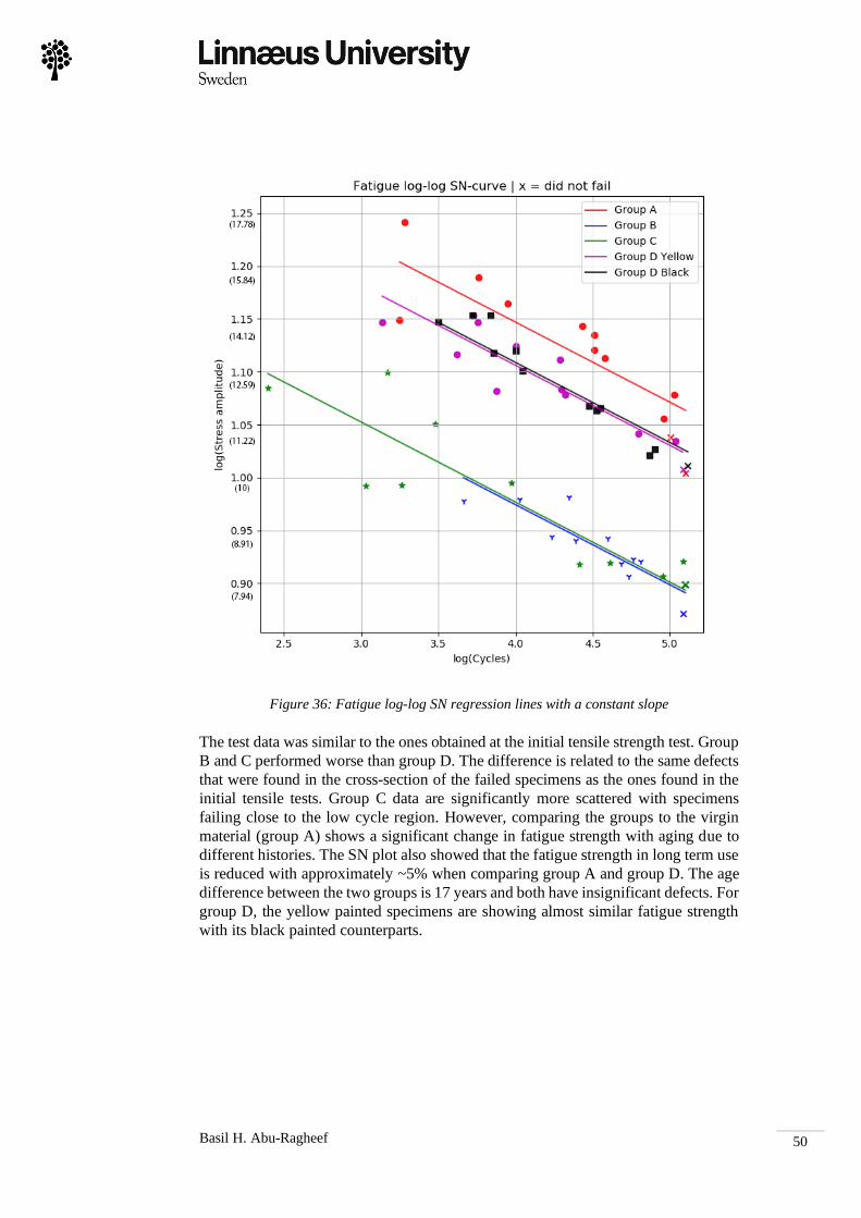
Basil H. Abu-Ragheef
50
Figure 36: Fatigue log-log SN regression lines with a constant slope
The test data was similar to the ones obtained at the initial tensile strength test. Group
B and C performed worse than group D. The difference is related to the same defects
that were found in the cross-section of the failed specimens as the ones found in the
initial tensile tests. Group C data are significantly more scattered with specimens
failing close to the low cycle region. However, comparing the groups to the virgin
material (group A) shows a significant change in fatigue strength with aging due to
different histories. The SN plot also showed that the fatigue strength in long term use
is reduced with approximately ~5% when comparing group A and group D. The age
difference between the two groups is 17 years and both have insignificant defects. For
group D, the yellow painted specimens are showing almost similar fatigue strength
with its black painted counterparts.
Basil H. Abu-Ragheef
51
The log-log S-N plots with confidence intervals shown in figure 37 and appendix 3
shows a 95% confidence level around the regression line. Differences can be observed
where the black painted specimens of group D have lower spread and significantly
higher life at the same stress level compared to its yellow counterparts. The spread in
group A is caused by selecting a high stress amplitude. The first starting test was taken
as 75% of the ultimate stress value obtained in the initial uniaxial tensile tests, later
that was changed to 66% to avoid fatigue failure at the low-cycle region. Due to
limited number of specimens, the results are kept as it is. The confidence intervals
were calculated by means of bootstrapping. This has been carried out using a Python
routine as shown in appendix 5.

Basil H. Abu-Ragheef
52
Figure 37: Confidence intervals of different groups (See also Appendix 3).

Basil H. Abu-Ragheef
53
5.3 Visual Analysis of Specimens After investigating and comparing the cross-section of the failed specimens and the
sheets that were it cut from, defects have been identified in the batches with
unexpected results. The defects can be categorized into:
• Processing defects, where the material has been defected during its molding
process.
• Usage defects, where the material is defected during its service period.
These categorizations have been concluded while examining the defects in all the
specimens and test materials. Samples from the defects are shown in the figures 38,
39, and 41.
Figure 38: Specimens B_F_Y_18 (first), B_F_Y_21 (second) showing bubble-like voids in its
bulk.

Basil H. Abu-Ragheef
54
All specimens from group B showed bubble-like defects in its bulk. These defects are
possibly generated during reaction injection molding processes where two liquid
monomers are mixed together and cured inside a mold in order to manufacture
pDCPD. For this case, these parts where molded with a RIM process. After reviewing
some related literature (Telene®, 2019; Teixeira et al., 2010; Rudd et al., 1997; Haagh
et al., 1996), the following reasons are assumed:
• Air bubbles could be formed due to boiling or formation of gas inside the
mold.
• Air could have entered the mold through a two-phase flow during injection.
• The mold was not made to allow flash areas to act as vents.
• The mold was not purged properly prior to injection
• The mold was not designed properly in terms of air vents.
The supposed bubbles/air-pockets could have possibly acquired its elongated shape
from the acting shear force during molding. It might have also occurred due to poor
and unstable thermodynamic conditions inside the mold. These conditions can allow
the formation of elongational forces that stretch the unmixed fluids (Bärwinkel et al.,
2016).
A second batch (Group C) showed different defects for all of its specimens. However,
these parts were cut from the hood of a heavy-duty vehicle covering high temperature
heat sources such as the engine and the turbocharger (Volvo CE, 2019). These defects
were most likely generated due to heat. This conclusion was drawn for the following
reasons:
• Unlike group B (figure 38), when examining the back surface of this batch
under a digital microscope (figure 41), it shows too many pores and cracks
on it that lead to the decay lines shown in figure 39.
• The tensile tests showed a pronounced brittle behavior for this group which,
alongside with the microcracks on the surface, are prime consequence of
thermal degradation (Write, 2001; Lampman, 2003).

Basil H. Abu-Ragheef
55
Figure 39: Specimens C_F_BK_31 (first) and C_F_BK_35(second) showing Thermal
defects in its bulk.
Micro cracks can also be seen in the back surface of D Black group where it is more
prone to heating and thermal degradation due to its color. However, it is less intense
than group C (See figure 41). Specimens from group A and D showed no defects
except for some cracks in D group. The figure below shows the clean cuts of samples
from both groups:

Basil H. Abu-Ragheef
56
Figure 40: Clean cuts of A_F_Y_8 (above) and D_F_BK_56 (below) showing no defects.

Basil H. Abu-Ragheef
57
Back surface of panel B
Back surface of panel C
Back surface of panel D Black
Figure 41: Back surface of B, C, and D_BK from above correspondingly. Images taken with
magnification of x65

Basil H. Abu-Ragheef
58
5.4 Viscoelastic Behaviors
5.4.1 Creep Behavior
All creep tests have been carried out at the load levels of: 1500, 1350, and 1200 N,
except for specimen B, where the loads were: 1400, 1200, and 1000 N. The lower test
levels are due to the defects and low stress at failure found in group B. The results are
plotted as strain-time and modulus-time curves. The modulus in this case is the creep
modulus which is the ratio between the fixed stress value and the current strain at a
specific time. The results for the first load levels are shown in figure 42 and 43, the
rest of the results in Appendix 3.
Figure 42: Creep curves for different age levels

Basil H. Abu-Ragheef
59
Figure 43: Creep curves for different age levels
Interestingly, physical aging showed minor effect on the creep data in terms of initial
strain response. Black panels specimens showed a significantly larger strain for the
same load. Different viscous deformation can be observed in figure 42 between group
C and the black painted specimens of group D, where group C strain is higher than
group D. Same behavior can be seen for groups A and D Yellow. However, these
viscous deformations can be more distinct at longer creep times. Despite being
subjected to lower force, group B has the highest strain rate that can be assumed to be
due to its defected and voided bulk. The same results can be observed at the other
load levels (see Appendix 3).
Viscoelastic behavior can be represented with spring and dashpot systems
(Bergström, 2015; Ward et al., 2004). The immediate deformation rise can be
represented with a spring system while the retardation happening afterwards can be
represented with a Kelvin-Voigt parallel spring-dashpot system. The gradual increase
in strain is the result of the slow deformation of the dashpot. This system can be
represented visually as follows:

Basil H. Abu-Ragheef
60
Figure 44: The spring-dashpot system that represents the creep deformation
This rheological model is called the Zener body or Three-Element model body which
consists of a spring (Hooke’s body) connected to a Kelvin-Voigt body in series
(Ottosen et al., 2005; Moczo et al., 2006). The constitutive relation of this model is
given as (Kelly, 2019):
𝜎 +
𝜂
𝐸1 + 𝐸2�̇� =
𝐸1𝐸2
𝐸1 + 𝐸2휀 +
𝜂𝐸1
𝐸1 + 𝐸2휀̇
(58)
The response of this model can be given through solving the differential equation by
specifying the stress or strain. This assumed model suggests that response will be
elastic to instantaneous loading and it will only suffer from primary creep (Ottosen et
al., 2005).
5.4.2 Cyclic Stress and Strain Behavior
During fatigue tests, when applying a sinusoidal stress, the strain response always
lagged behind the stress, this lag is caused by the viscoelastic properties of the
material. The time difference Δt has been calculated after normalizing the stress and
strain signal with a python routine (Appendix 5) and calculating the difference in time
and the phase difference ẟ. The loss ratio, complex, storage, and loss moduli has been
obtained by using the equations (43), (44), (45), and (48). The mentioned quantities
are functions of frequency and temperature (Bergström, 2015). Thus, it is important
to note that the frequency of this test was 15 Hz with varying temperatures due to
thermal fatigue.

Basil H. Abu-Ragheef
61
Figure 45: The lag between stress-strain responses
Figure 46: Damping ratio tan(ẟ) change with age
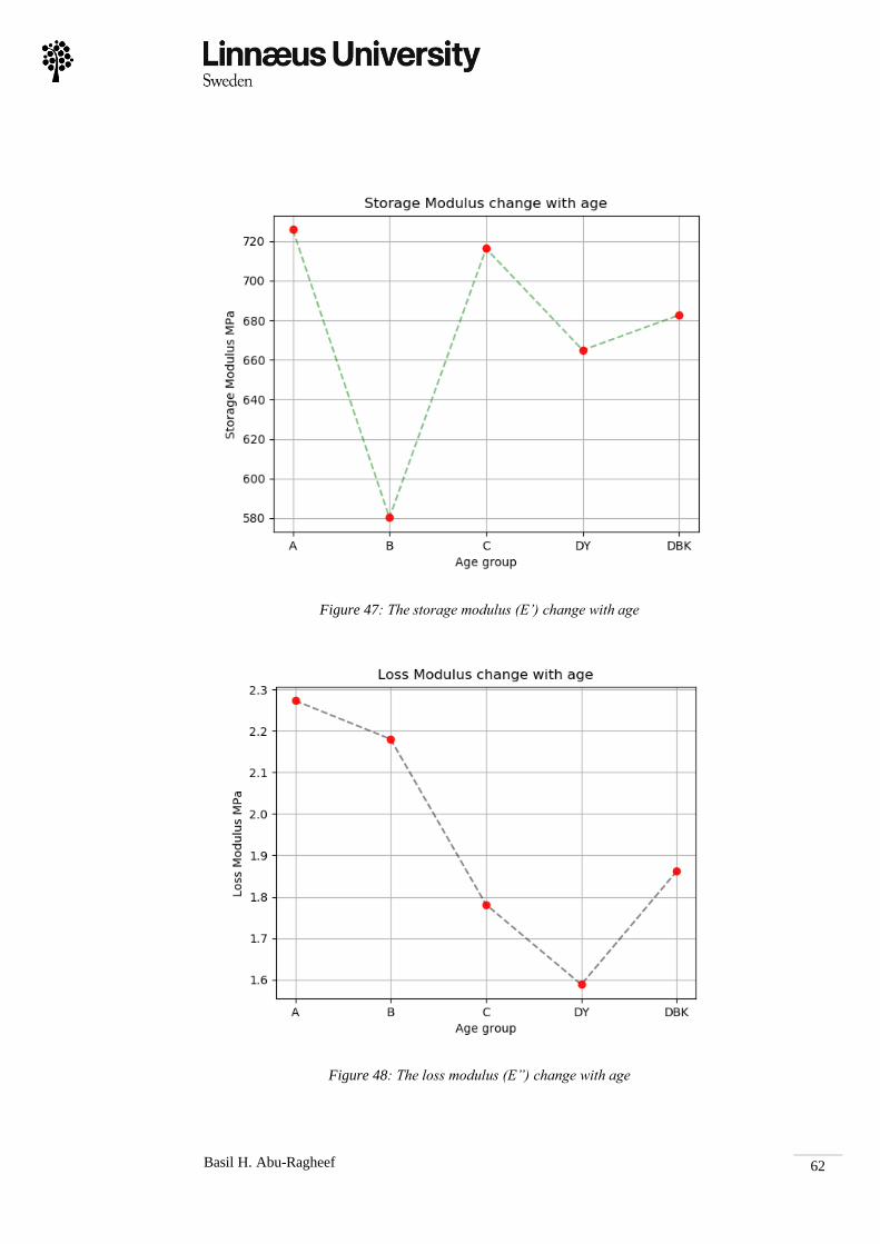
Basil H. Abu-Ragheef
62
Figure 47: The storage modulus (E’) change with age
Figure 48: The loss modulus (E”) change with age

Basil H. Abu-Ragheef
63
As seen in the figures, the loss ratio or damping ratio is relatively low in pDCPD due
to its stiffness and relative brittleness. It has high storage capacity and very low loss
modulus (energy dissipation) in general. The damping ratio can be used as a measure
of elasticity. If a material has a reduced damping ratio, it means that it is moving
towards a purely elastic material.
This occur due to the reduction in loss modulus and or increase in the storage modulus
(Menard et al., 2006). Storage and loss modulus results figures show that group A
has very high energy storage capacity (elastic response capacity) in the same time
relatively high energy loss capacity (viscous response). Excluding group B, the
change in storage and loss modulus is significant between group A, C and D. The
difference between black and yellow panels specimens suggest that the material tend
toward more elastic and less viscous behaviors, unlike group B where it has a
dominant viscous behavior. That can be observed in creep results as well where group
B preformed the most viscous response.

Basil H. Abu-Ragheef
64
5.5 Thermal Behavior During Cyclic Stress Tests Temperature data during fatigue testing showed a steady linear increase in
temperature with the increase of stress. The purpose of capturing temperature data
during fatigue tests was to make sure that the temperature raised will not reach closed
to the transition temperature Tg that might alter the physical aging conditions of the
specimens or reverse it. The results of the temperature (Shown in details in Appendix
2&3) showed a maximum temperature range of 33-41 ºC for all specimens, which is
well below the critical level Tg of pDCPD which is 155 ºC (Telene®, 2019). However,
the measured temperature is on the surface. The temperature in the bulk around the
crack region of the specimens was often 10-30 ºC higher than the surface as shown in
the thermal image samples in figures 50, 51, and 52.
Figure 49: Temperature rise for different stress levels during cyclic testing of group A.

Basil H. Abu-Ragheef
65
Figure 50: Thermal image from specimen B_F_Y_30 during rapture from cyclic loading
Figure 51: Thermal image from specimen D_F_Y_43 after rapture from cyclic loading

Basil H. Abu-Ragheef
66
Figure 52: Thermal image from specimen D_F_Y_44 during rapture from cyclic loading
During testing it is possible to predict where the fracture will occur from temperature
increase on the surface’s hotspots. The area with the highest temperature in the
specimen is the one that most likely to be fractured. This can be linked to the crack
initiation and propagation phase where stress concentrations start to form (Sauer et
al., 1980). The maximum recorded temperature during rapture was 59 ºC, still lower
than the referenced Tg. However, more research is required to determine what is the
actual Tg of the tested materials and if it changed with age. The plastic material was
cut from heavy duty trucks stored in open air during harsh Scandinavian winters. It is
also important to determine T𝜷 of the material as the actual range of temperature in
which physical aging occurs is between T𝜷 and Tg (Perepechko, 1980; Sturik, 1977).
The temperature generated during the test can also be linked with the loss modulus
and also with other factors such as frequency and stress level as discussed in section
2.6.1.

Basil H. Abu-Ragheef
67
6 Discussion
The purpose of this research was to investigate the mechanical properties of
polyDicyclopentadiene (pDCPD) subjected to aging. The research questions have
been explained with considrations both theory and experiment. The theory explained
the different degradation processes that occurs in polymers in general and those which
could occur in cross-linked thermosets similar to pDCPD. The experimental part has
used state-of-the-art equipment to investigate different aspects such as tensile
strength, fatigue, creep, viscoelastic and dynamic properties of the material. Different
properties and behaviors have been identified for each age group. The results have
been analyzed and linked to theory.
However, from the results obtained, it is hard to distinct between each degradation
effect except for group C where thermal degradation is severe and more pronounced
than others. For group D, physical aging can also be noticed and performance
difference between painted panels in different colors is observed. The black painted
specimens performed lower due to higher thermal- and photo-degradation. Moreover,
group D was covered with biofilms on its surface (See Appendix 1) and all aged panel
was in contact with water and snow and was most likely subjected to chemical
degradation due to hydrolysis and water absorption during their service. It is unclear
how these factors affected the polymer material independently. For group B the aging
effects are hard to verify due to its defects that are most likely due to flaws in
manufacturing. Thus, it is improper to compare it to other groups.
This research did not take into account other climates and working environments, e.g.
desert or tropical environments. These results are only valid for the cold and wet
Scandinavian climate. More research could have been done to investigate how the
material would behave in different temperatures and humidity conditions. Aging
could be simulated through accelerated aging techniques to construct master curves
and predict the performance for different periods of time. Another overlooked aspect
of this research is not finding the actual T𝜷 and Tg of the material and if it has changed
with time. As the results has shown some properties such as the Young’s modulus of
the material is different than what it is stated in datasheets and literature. To find
transition temperatures, a dynamic mechanical analysis test (DMA) needed to record
the change of tan(ẟ) with temperature to identify the different transition phases.
Another question that could be raised is to conclude if the temperature rise from
fatigue test actually affects the data related to physical aging, since physical aging is
sensitive to temperature and is thermoreversible.
An implicit aim of this research is to verify whether the material is suitable for a self-
carrying structure for the vehicle exterior shell. For this purpose, it is important to
understand the processing conditions and possible defects that can arise from flawed
manufacturing. However, it was not possible to obtain the history of the molding
process of these defected parts ahead of time. Thus, it would be too early to make
valid arguments for identifying the roots causes of the problem.
The results of group B raises the following questions: What causes these defects?
How frequent does it happen? And how to eliminate or reduce it? Some possible
assumptions were given in the result section to explain those defects. In terms of

Basil H. Abu-Ragheef
68
group B, it was assumed that the defects were formed by possible bubbles during
manufacturing and a hypothesis on its shape has been made. However, that hypothesis
is only proven on immiscible polymers mixes in injection molding process and not
bubbles. It needs to be validated with further research. In regarding Group C, its
defects were more likely to have happened due to heat generated during its service
time. The panels of group C were cut from a hood covering the engine. Its defects
could be prevented with a second protective layer of paint on the back surface of the
panels to protect it from the heat produced from the heat source. However, these
assumptions are based on visual reasoning, tacit knowledge, and literature review and
more research is needed to confirm the provided hypotheses.
All the test settings where based on testing standards provided either by ISO or
ASTM. The research was conducted in a way to meet the minimum accuracy
requirements provided in those guidelines. 12 specimens were used for each group in
fatigue testing, three for each load level with a total of 4 load levels. However, the
fatigue test for group A could have been done better by organizing the load levels in
a correct manner to reduce spread in the data. Other groups were more organized as
the fatigue stresses became more known to the tester. Three specimens were used
during uniaxial tensile testing, however, the minimum required is 5. The limited
number of specimens and time was another constraint during this research.
In this research, the creep test period was 10 minutes and the specimen only suffered
primary creep. A much longer test with specialized equipment is needed with more
specimens in order to have accurate creep results. The viscoelastic properties were
calculated using the sinusoidal stress signals from the fatigue tests. A more proper
way to calculate those properties is through dynamic mechanical analysis (DMA)
tests using specialized DMA hardware. The aim of the tests carried out was to have a
sense on how the viscoelastic behavior may change with age.

Basil H. Abu-Ragheef
69
7 Conclusion
Polymers can undergo many degradation processes. Time-dependent degradations
such as physical aging are one of them, and it can have a significant negative effect
on the mechanical properties as illustrated in the results obtained from specimens
group A (2018) and D (2002). Other degradation processes such as thermo- and
photo- oxidation are equally as important.
The test results of group C (2012) showed how heat sources can drastically damage
the material and reduce its performance. However, differences in group D between
the black and yellow painted material are also observed. Microcracks are formed on
the surface of the black-painted materials that affect fatigue life and endurance limit.
Fatigue life has shown a reduction of ~5% between the yellow panels of group A and
group D.
The viscoelastic behavior has been observed in both cyclic test and creep tests.
Dynamic moduli and damping ratios have been obtained. Creep data indicated a
longer initial strain response in black painted panels due to thermal and photo
degradation. However, the increase of strain due to viscous deformation are slower in
old panels than new ones. Thermal data recorded during cycling loading showed that
temperature in the bulk of the crack region of the specimens were 10-30 ºC higher
than its surface. However, it showed no significant increase to temperature close to
Tg of pDCPD.
The results also showed that different defects can arise in the material. Group C
suffered from severe thermal degradation due to its placement above a heat source.
Group B are suspected to have defects due to a flaw in manufacturing. Digital image
correlation system proved more credible in extracting strain data and calculating
Young’s modulus. The research questions and aim of this research has been fulfilled
with respect to constraints and limitations.
Basil H. Abu-Ragheef
70
References
1. ADMET (2019). Effect of Specimen Geometry on Tensile Testing Results.
[online] Available at: https://www.admet.com/effect-specimen-geometry-
tensile-testing-results/ [Accessed 14 May. 2019].
2. Affonso, L. O. A. (2006). Fatigue Fractures. Machinery Failure Analysis
Handbook, 43–53.
3. Ashter, S. A. (2013). Thermoforming of Single and Multilayer Laminates:
Plastic Films Technologies, Testing, and Applications. William Andrew.
4. ASTM D7791 − 17. (2017). Standard Test Method for Uniaxial Fatigue
Properties of Plastics. ASTM International (American Society for Testing
and Materials).
5. Barbero, E. J., & Ford, K. J. (2004). Equivalent time temperature model for
physical aging and temperature effects on polymer creep and relaxation.
Journal of engineering materials and technology, 126(4), 413-419.
6. Bärwinkel, S., Seidel, A., Hobeika, S., Hufen, R., Mörl, M., & Altstädt, V.
(2016). Morphology Formation in PC/ABS Blends during Thermal
Processing and the Effect of the Viscosity Ratio of Blend Partners.
Materials, 9(8), 659. doi:10.3390/ma9080659
7. Bayoumi, M. R., & Abdellatif, A. K. (1995). Effect of surface finish on
fatigue strength. Engineering Fracture Mechanics, 51(5), 861–870.
8. Bergström, J. S. (2015). Mechanics of solid polymers: theory and
computational modeling. William Andrew.
9. Borman, Stu. (2014). Polymers and composites made incredibly cheaply.
[online] Available at: https://cen.acs.org/materials/polymers/Polymers-
composites-made-incredibly-cheaply/96/i20 [Accessed 26 Feb. 2019].
10. Boyer, R. F. (1968). Dependence of mechanical properties on the molecular
motion in polymers. Polymer Engineering & Science, 8(3), 161-185.
11. Bueche, F. (1953). Segmental Mobility of Polymers Near Their Glass
Temperature. The Journal of Chemical Physics, 21(10), 1850–1855.
12. Chen, J., Burns, F. P., Moffitt, M. G., & Wulff, J. E. (2016). Thermally
Crosslinked Functionalized Polydicyclopentadiene with a High T g and
Tunable Surface Energy. ACS Omega, 1(4), 532-540.
13. Chen, J., Burns, F. P., Moffitt, M. G., & Wulff, J. E. (2016). Thermally
Crosslinked Functionalized Polydicyclopentadiene with a High Tg and
Tunable Surface Energy. ACS Omega, 1(4), 532–540.
14. Cintrón, Rommel & Saouma, V. (2008). Strain Measurements with Digital
Image Correlation System Vic-2D.
15. Dodiuk, H., & Goodman, S. H. (Eds.). (2013). Handbook of thermoset
plastics. William Andrew.
16. Driscoll S. B. (1998). The Basics of Testing Plastics: Mechanical
Properties, Flame Exposure, and General Guidelines. ASTM Manual
Series: MNL35
17. EERE. (2019). J. Lightweight materials for cars and trucks. Office of
Energy Efficiency & Renewable Energy. [online] Available at:

Basil H. Abu-Ragheef
71
https://www.energy.gov/eere/vehicles/lightweight-materials-cars-and-trucks
[Accessed 11 March. 2019].
18. Ekberg, A. (1998) Fatigue crack propagation, lecture notes, Fatigue and
Fracture Analysis MHA140. Chalmers University of Technology, [online]
Available at: http://www.am.chalmers.se/~anek/teaching/fatfract/ [Accessed
23 March. 2019].
19. EngApplets (2019) Mohr's Circle for 2-D Stress Analysis, [online]
Available at:
http://www.engapplets.vt.edu/Mohr/java/nsfapplets/MohrCircles2-
3D/Theory/theory.htm/ [Accessed 14 May. 2019].
20. Erhard, G., & Thompson, M. (2006). Designing with plastics. Munich,
Germany: Hanser.
21. Ferry, J. D. (1980). Viscoelastic properties of polymers. 3rd Edition. John
Wiley & Sons.
22. Fotopoulou, K. N., & Karapanagioti, H. K. (2017). Degradation of Various
Plastics in the Environment. The Handbook of Environmental Chemistry.
23. Fox, J. (2002). Bootstrapping Regression Models. Department of Statistics.
Stanford University. Retrieved from:
http://statweb.stanford.edu/~tibs/sta305files/FoxOnBootingRegInR.pdf
24. Grabowski, L., Baier, A., & Sobek, M. (2017). Molding of strength testing
samples using modern PDCPD material for purpose of automotive industry.
IOP Conference Series: Materials Science and Engineering, 227, 012051.
25. Haagh, G. A. A. V., Peters, G. W. M., & Meijer, H. E. H. (1996). Reaction
injection molding: Analyzing the filling stage of a complex product with a
highly viscous thermoset. Polymer Engineering & Science, 36(20), 2579-
2588.
26. Hensley, S., Christensen, M., Small, S., Archer, D., Lakes, E., & Rogge, R.
(2017). Digital image correlation techniques for strain measurement in a
variety of biomechanical test models. Acta of bioengineering and
biomechanics, 19(3).
27. Hertzberg, R. W., Vinci, R. P., Hertzberg, J. L. (2012). Deformation and
fracture mechanics of engineering materials. 5th Edition Wiley.
28. Hughes, J. (2005). MECHANICAL RESONANCE. Department of Physics
and Astronomy Serin Physics Laboratory. The State University of New
Jersey. Retrieved from:
http://www.physics.rutgers.edu/~jackph/2005s/PS02.pdf
29. Hutchinson, J. M. (1995). Physical aging of polymers. Progress in polymer
science, 20(4), 703-760.
30. ISO 20753:2018. Plastics — Test specimens. International Organization for
Standardization (ISO).
31. ISO 2818:2018. Plastics — Preparation of test specimens by machining.
International Organization for Standardization (ISO).
32. ISO 527-1:2012. Plastics – Determination of tensile properties –Part 1:
General principles. International Organization for Standardization (ISO).
33. ISO 899-1:2017. Plastics — Determination of creep behaviour —Part 1:
Tensile creep. International Organization for Standardization (ISO).

Basil H. Abu-Ragheef
72
34. Jenkins, A. D. (1996). Glossary of basic terms in polymer science. Pure and
Applied Chemistry. 68 (12): 2287–2311.
35. Jeremy Orloff and Jonathan Bloom. (2014). Bootstrap confidence intervals,
Class 24, 18.05. Massachusetts Institute of Technology Cambridge.
Retrieved from: https://ocw.mit.edu/courses/mathematics/18-05-
introduction-to-probability-and-statistics-spring-
2014/readings/MIT18_05S14_Reading24.pdf
36. Kelly, P. (2019) Solid Mechanics Part I: An Introduction to Solid
Mechanics. Mechanics Lecture Notes. The University of Auckland.
Retrieved from:
http://homepages.engineering.auckland.ac.nz/~pkel015/SolidMechanicsBoo
ks/Part_I/BookSM_Part_I/10_Viscoelasticity/10_Viscoelasticity_03_Rheol
ogical.pdf
37. Klosiewicz, D. (1984). Patent No. US4436858A. The United States.
[Accessed 26 Feb. 2019].
38. Kulkarni, G. S. (2018). Introduction to Polymer and Their Recycling
Techniques. Recycling of Polyurethane Foams, 1–16.
39. Lakes, R. (2019). Viscoelasticity Notes adapted from Viscoelastic Materials
Book. University of Wisconsin. Retrieved from:
http://silver.neep.wisc.edu/~lakes/VEnotes2.html [Accessed 31st May.
2019].
40. Lampman, S. (2003). Characterization and failure analysis of plastics. Asm
International.
41. Landel, R. F., & Nielsen, L. E. (1993). Mechanical properties of polymers
and composites. CRC press.
42. Le Gac, P. Y., Choqueuse, D., Paris, M., Recher, G., Zimmer, C., & Melot,
D. (2013). Durability of polydicyclopentadiene under high temperature,
high pressure and seawater (offshore oil production conditions). Polymer
degradation and stability, 98(3), 809-817.
43. Malkin, A. Y., & Isayev, A. I. (2012). VISCOELASTICITY. Rheology
Concepts, Methods, and Applications, 43–126.
44. Maurer, M. T. (2017). Statistical Analysis of Fatigue Data in Mechanical
Engineering. A master thesis written at the Institute of Statistics, Graz
University of Technology. Retrieved from:
https://diglib.tugraz.at/download.php?id=5a33ac2d24c7e
45. Maxwell A. S., Broughton W. R., Dean G., Sims G. D. (2005). Review of
Accelerated Ageing Methods and Lifetime Prediction Techniques for
Polymeric Materials. [online] Available at:
https://www.researchgate.net/publication/283345000_Review_of_Accelerat
ed_Ageing_Methods_and_Lifetime_Prediction_Techniques_for_Polymeric
_Materials [Accessed 9 April. 2019].
46. McKeen, L. W. (2016). Fatigue and tribological properties of plastics and
elastomers. William Andrew.
47. McKenna, G.B., (1989). Glass formation and glassy behavior. Pergamon
Press plc, Comprehensive Polymer Science: The Synthesis,
Characterization, Reactions & Applications of Polymers., 2, pp.311-362.

Basil H. Abu-Ragheef
73
48. Menard, K. P., & Menard, N. (2006). Dynamic mechanical analysis.
Encyclopedia of Analytical Chemistry: Applications, Theory and
Instrumentation, 1-25.
49. Minervino, M., Gigliotti, M., Lafarie-Frenot, M. C., & Grandidier, J. C.
(2013). The effect of thermo-oxidation on the mechanical behaviour of
polymer epoxy materials. Polymer Testing, 32(6), 1020–1028.
50. Moczo, P., Kristek, J., & Franek, P. (2006). Lecture Notes on Rheological
Models. DAPEM FMPI, Comenius University. Retrieved from:
http://www.earthphysics.sk/mainpage/stud_mat/Moczo_Kristek_Franek_Rh
eological_Models.pdf
51. Mullins, M. J., Liu, D., & Sue, H. J. (2018). Mechanical properties of
thermosets. In Thermosets (pp. 35-68). Elsevier.
52. Ottosen, N. S., & Petersson, H. (1992). Introduction to the Finite Element
Method. Prentice-Hall.
53. Ottosen, N. S., & Ristinmaa, M. (2005). The mechanics of constitutive
modeling. Elsevier.
54. Pan, J. (2015). Modelling degradation of semi-crystalline biodegradable
polyesters. Modelling Degradation of Bioresorbable Polymeric Medical
Devices, 53–69.
55. Pedersen, M. (2018). Introduction to Metal Fatigue. Technical Report
Mechanical Engineering, 5(11), 91. Retrieved from:
https://tidsskrift.dk/me/article/view/110952
56. PEMRG. (2017). Plastics – the Facts 2017 An analysis of European
plastics production, demand and waste data. [online] Available at:
https://www.plasticseurope.org/application/files/5715/1717/4180/Plastics_t
he_facts_2017_FINAL_for_website_one_page.pdf [Accessed 5 March.
2019].
57. Perepechko, I. (1980). Low-temperature properties of polymers. Pergamon.
58. Pervaiz, M., Panthapulakkal, S., Birat, K. C., Sain, M., & Tjong, J. (2016).
Emerging trends in automotive lightweighting through novel composite
materials. Materials Sciences and Applications, 7(01), 26.
59. Plastics Market Watch. (2016). Automotive Recycling: Devalued is now
Revalued. [online] Available at:
https://www.plasticsindustry.org/sites/default/files/2016-03256-SPI-PMW-
Auto-Recycle-web_0.pdf [Accessed 5 March. 2019].
60. Pradeep, S. A., Iyer, R. K., Kazan, H., & Pilla, S. (2017). Automotive
Applications of Plastics: Past, Present, and Future. Applied Plastics
Engineering Handbook, 651–673.
61. Python Software Foundation, (2019). https://www.python.org/ [Accessed 10
May. 2019].
62. RIMTEC. (2019). Molding Process of Telene®. [online] Available at:
http://www.rimtec.co.jp/en/telene/process.html [Accessed 26 Feb. 2019].
63. Rosato, D. V. (2003). Plastics engineered product design. Elsevier.
64. Roylance, D. (2001). Fatigue. Department of Materials Science and
Engineering. Massachusetts Institute of Technology Cambridge, MA 02139.
Retrieved from: http://web.mit.edu/course/3/3.11/www/modules/fatigue.pdf

Basil H. Abu-Ragheef
74
65. Rudd, C. D., Long, A. C., Kendall, K. N., & Mangin, C. (1997). Liquid
moulding technologies: Resin transfer moulding, structural reaction
injection moulding and related processing techniques. Elsevier.
66. Rudin, A. (1998). Elements of Polymer Science & Engineering: An
Introductory Text and Reference for Engineers and Chemists. Elsevier.
67. Sang, L., Wang, C., Wang, Y., & Wei, Z. (2017). Thermo-oxidative ageing
effect on mechanical properties and morphology of short fibre reinforced
polyamide composites – comparison of carbon and glass fibres. RSC
Advances, 7(69), 43334–43344.
68. Sauer, J. A., & Richardson, G. C. (1980). Fatigue of polymers. International
journal of fracture, 16(6), 499-532.
69. Schreier, H., Orteu, J.-J., & Sutton, M. A. (2009). Image Correlation for
Shape, Motion and Deformation Measurements.
70. Serrenho, A. C., Norman, J. B., & Allwood, J. M. (2017). The impact of
reducing car weight on global emissions: the future fleet in Great Britain.
Philosophical Transactions of the Royal Society A: Mathematical, Physical
and Engineering Sciences, 375(2095), 20160364.
71. Shah, V. (2007). Handbook of plastics testing and failure analysis (Vol.
21). John Wiley & Sons.
72. Simons, R., Guntari, S. N., Goh, T. K., Qiao, G. G., & Bateman, S. A.
(2012). Poly (dicyclopentadiene)‐montmorillonite nanocomposite formation
via simultaneous intergallery‐surface initiation and chain crosslinking
using ROMP. Journal of Polymer Science Part A: Polymer Chemistry,
50(1), 89-97.
73. Struik, L. C. E. (1977). Physical aging in amorphous polymers and other
materials.
74. Teixeira, A., & Ribeiro, B. (2010). USE OF DCPD/RIM ON EXTERIOR
PANELS FOR THE AUTOMOTIVE INDUSTRY.
75. Telene®. (2019) TELENE PART AND MOULD DESIGN GUIDE. Version
VA – WM – 2015/02. [online] Available at:
https://www.telene.com/pdf/TechnicalBulletins/Telene-Part-and-Mould-
Design-Guide.pdf [Accessed 10 May. 2019].
76. The Henry Ford. (2019). Soybean Car. [online] Available at:
https://www.thehenryford.org/collections-and-research/digital-
resources/popular-topics/soy-bean-car [Accessed 11 March. 2019].
77. Tokiwa, Y., Calabia, B., Ugwu, C., & Aiba, S. (2009). Biodegradability of
Plastics. International Journal of Molecular Sciences, 10(9), 3722–3742.
78. Vallons, K. A. M., Drozdzak, R., Charret, M., Lomov, S. V., & Verpoest, I.
(2015). Assessment of the mechanical behaviour of glass fibre composites
with a tough polydicyclopentadiene (PDCPD) matrix. Composites Part A:
Applied Science and Manufacturing, 78, 191–200.
79. Van Dijk, M. A., & Wakker, A. (1998). Concepts in polymer
thermodynamics (Vol. 2). CRC Press. P.5-6
80. Volvo CE. (2019). Volvo Construction Equipment AB, Braås, Sweden.
81. Walpole, R. E., Myers, R. H., Myers, S. L., & Ye, K. (2017). Probability
and statistics for engineers and scientists (Vol. 9). New York: Macmillan.

Basil H. Abu-Ragheef
75
82. Ward, I. M., & Sweeney, J. (2004). An introduction to the mechanical
properties of solid polymers. John Wiley & Sons. P.203-205
83. Wright, D. (2001). Failure of plastics and rubber products: causes, effects
and case studies involving degradation. iSmithers Rapra Publishing.
84. Wu, X. (2019). Chapter 6: Curve Fitting. Department of Electrical &
Computer Engineering. McMaster University. Retrieved from:
http://www.ece.mcmaster.ca/~xwu/part5.pdf [Accessed 9 May. 2019].
85. Wypych, G. (2016). Handbook of polymers. Elsevier.
86. Yabannavar, A. V., & Bartha, R. (1994). Methods for assessment of
biodegradability of plastic films in soil. Appl. Environ. Microbiol., 60(10),
3608-3614.
87. Yang, B., Wang, G., Peter, W. H., Liaw, P. K., Buchanan, R. A., Fielden, D.
E., … Klarstrom, D. L. (2004). Thermal-imaging technologies for detecting
damage during high-cycle fatigue. Metallurgical and Materials Transactions
A, 35(1), 15–23.

Basil H. Abu-Ragheef
76
Appendix 1: Material Sheets
Figure 53: Panel D Yellow
Figure 54: Panel C

Basil H. Abu-Ragheef
77
Figure 55: Panel B
Figure 56: Panel D Black

Basil H. Abu-Ragheef
78
Appendix 2: Detailed Spreadsheet for each specimen
ID
Specimen ID Gauge Width
Gauge Thick
Initial temp.
final temp.
max force
min force
mean ampl freq
A_S_Y_1_20190506 10.07 4.83 - - - - - - -
D_S_BK_2_20190506 10.13 4.8 - - - - - - -
B_S_Y_3_20190506 10.17 5.14 - - - - - - -
D_S_Y_4_20190506 10.08 5.25 - - - - - - -
C_S_BK_5_20190506 10.1 4.71 - - - - - - -
A_F_Y_6_20190509 10.07 4.58 23.7 37.2 1780 178 979 801 10
A_F_Y_7_20190509 10.08 4.64 26.2 37.9 1600 160 880 720 10
A_F_Y_8_20190509 10.07 4.6 23.3 35.7 1500 150 825 675 10
A_F_Y_9_20190509 10.07 4.62 25.8 28.3 1125 112.5 618.75 506.25 10
A_F_Y_10_20190509 10.12 4.64 23.8 30.8 1350 135 742.5 607.5 10
A_F_Y_11_20190509 10.17 4.64 24.1 33.1 1425 142.5 783.75 641.25 10
A_F_Y_12_20190510 10.11 4.56 24.6 31.5 1350 135 742.5 607.5 10
A_F_Y_13_20190510 10.14 4.58 24.4 37.1 1450 145 797.5 652.5 10
A_F_Y_14_20190510 10.09 4.58 25.9 34.8 1425 142.5 783.75 641.25 10
A_F_Y_15_20190513 10.06 5.06 24.1 33.1 1350 135 742.5 607.5 15
A_F_Y_16_20190513 10.06 4.94 24.2 31.3 1250 125 687.5 562.5 15
A_F_Y_17_20190513 10.1 5.31 24.2 30.1 1200 120 660 540 15
B_F_Y_18_20190514 10.11 5.15 24.1 32.5 1100 110 605 495 15
B_F_Y_19_20190514 10.09 5.14 23.9 31.1 1100 110 605 495 15
B_F_Y_20_20190514 10.12 5.16 24.3 33.1 1100 110 605 495 15
B_F_Y_21_20190514 10.07 5.1 23.8 30.4 1000 100 550 450 15
B_F_Y_22_20190514 10.15 5.1 24.4 31.7 1000 100 550 450 15
B_F_Y_23_20190514 10.08 5.12 23.8 27.3 850 85 467.5 382.5 15
B_F_Y_24_20190514 10.04 5.14 25.3 30.7 1000 100 550 450 15
B_F_Y_25_20190514 10.13 5.11 24.8 30.8 950 95 522.5 427.5 15
B_F_Y_26_20190515 10.04 5.13 24.1 29 950 95 522.5 427.5 15
B_F_Y_27_20190515 10.08 5.09 24.6 27.6 900 90 495 405 15
B_F_Y_28_20190515 10.07 5.14 25.2 29.6 925 92.5 508.75 416.25 15
B_F_Y_29_20190515 10.01 5.12 24.9 29.7 950 95 522.5 427.5 15
C_F_BK_30_20190515 10.14 4.76 23.7 37.7 1450 145 797.5 652.5 15
C_F_BK_31_20190515 10.1 4.82 24.3 29.2 1400 140 770 630 15

Basil H. Abu-Ragheef
79
C_F_BK_32_20190515 10.17 4.86 24.6 25.3 1300 130 715 585 15
C_F_BK_33_20190515 10.07 4.67 24.8 29.7 1150 115 632.5 517.5 15
C_F_BK_34_20190515 10.06 4.65 25.3 30.2 1150 115 632.5 517.5 15
C_F_BK_35_20190515 10.16 7.77 24.1 27.6 1150 115 632.5 517.5 15
C_F_BK_36_20190516 10.08 4.79 25.1 28.1 950 95 522.5 427.5 15
C_F_BK_37_20190516 10.09 4.76 25.3 29.1 950 95 522.5 427.5 15
C_F_BK_38_20190516 10.18 4.75 25.7 27.4 950 95 522.5 427.5 15
C_F_BK_39_20190516 10.07 4.78 24.7 26.7 900 90 495 405 15
C_F_BK_40_20190517 10.07 4.83 24.6 29.4 925 92.5 508.75 416.25 15
C_F_BK_41_20190517 10.07 4.88 24.9 26.7 900 90 495 405 15
D_F_Y_42_20190517 10.12 5.25 25.5 41.8 1650 165 907.5 742.5 15
D_F_Y_43_20190517 10.14 5.24 25.3 39.7 1650 165 907.5 742.5 15
D_F_Y_44_20190517 10.16 5.15 25.1 39.4 1650 165 907.5 742.5 15
D_F_Y_45_20190517 10.08 5.28 25.4 39.2 1525 152.5 838.75 686.25 15
D_F_Y_46_20190517 10.12 5.21 25.6 37.4 1525 152.5 838.75 686.25 15
D_F_Y_47_20190517 10.09 5.18 25.8 37.8 1525 152.5 838.75 686.25 15
D_F_Y_48_20190520 10.06 5.19 25.4 33.2 1400 140 770 630 15
D_F_Y_49_20190520 10.11 5.18 24.2 32 1400 140 770 630 15
D_F_Y_50_20190520 10.09 5.23 25.5 34.1 1400 140 770 630 15
D_F_Y_51_20190520* 10.13 5.27 25.7 31.7 1300 130 715 585 15
D_F_Y_52_20190520 10.08 5.17 23.5 29.5 1250 125 687.5 562.5 15
D_F_Y_53_20190520 10.09 5.28 24.6 29.3 1200 120 660 540 15
D_F_BK_54_20190520 10.06 4.76 24.7 36.1 1500 150 825 675 15
D_F_BK_55_20190521 10.06 4.75 24.1 34 1500 150 825 675 15
D_F_BK_56_20190521 10.09 4.78 24.6 33.8 1500 150 825 675 15
D_F_BK_57_20190521 10.11 4.75 25.3 33.8 1400 140 770 630 15
D_F_BK_58_20190521 10.15 4.75 24 35.6 1400 140 770 630 15
D_F_BK_59_20190521 10.14 4.76 25.3 33.9 1350 135 742.5 607.5 15
D_F_BK_60_20190521 10.17 4.77 24.7 31 1250 125 687.5 562.5 15
D_F_BK_61_20190521 10.08 4.84 23.4 30.9 1250 125 687.5 562.5 15
D_F_BK_62_20190521 10.13 4.77 25.7 31.1 1250 125 687.5 562.5 15
D_F_BK_63_20190521 10.14 4.81 25.1 29.7 1150 115 632.5 517.5 15
D_F_BK_64_20190521 10.11 4.81 25 29.7 1100 110 605 495 15
D_F_BK_65_20190521 10.08 4.8 24.7 28.7 1125 112.5 618.75 506.25 15
A_C_Y_66_20190530 10.06 4.91
1500
-
1350
-
1200
-
B_C_Y_67_20190530 10.14 5.12
1400
-

Basil H. Abu-Ragheef
80
1200
-
1000
-
C_C_BK_68_20190530 10.17 4.73
1500
-
1350
-
1200
-
D_C_Y_69_20190530 10.13 5.33
1500
-
1350
-
1200
-
D_C_BK_70_20190530 10.07 4.76
1500
-
1350
-
1200
-
A_S_Y_71_20190530 10.07 5.04
B_S_Y_72_20190530 10.12 5.13
C_S_BK_73_20190530 10.17 4.88
D_S_Y_74_20190530 10.18 5.19
D_S_BK_75_20190530 10.11 4.77
*Red ID means that the specimen did not break

Basil H. Abu-Ragheef
81
Appendix 3 Other test results
• Tensile tests
Figure 57: Third tensile test results

Basil H. Abu-Ragheef
82
• Fatigue tests
Figure 58: Results of the A_F_Y group
Figure 59: Results of the A_F_Y group

Basil H. Abu-Ragheef
83
Figure 60: Results of the B_F_Y group
Figure 61: Results of the B_F_Y group

Basil H. Abu-Ragheef
84
Figure 62: Results of the C_F_BK group
Figure 63: Results of the C_F_BK group

Basil H. Abu-Ragheef
85
Figure 64: Results of the D_F_Y group
Figure 65: Results of the D_F_Y group

Basil H. Abu-Ragheef
86
Figure 66: Results of the D_F_BK group
Figure 67: Results of the D_F_BK group

Basil H. Abu-Ragheef
87
• Creep results
Figure 68: Creep curve for force level 1200N
Figure 69: Creep modulus curve for force level 1200N

Basil H. Abu-Ragheef
88
Figure 70: Creep curve for force level 1350N
Figure 71: Creep modulus curve for force level 1350N

Basil H. Abu-Ragheef
89
Appendix 4: DIC system results for strain analysis

Basil H. Abu-Ragheef
90

Basil H. Abu-Ragheef
91

Basil H. Abu-Ragheef
92

Basil H. Abu-Ragheef
93

Basil H. Abu-Ragheef
94

Basil H. Abu-Ragheef
95

Basil H. Abu-Ragheef
96

Basil H. Abu-Ragheef
97

Basil H. Abu-Ragheef
98

Basil H. Abu-Ragheef
99
Appendix 5: Python Routines
All the routines made for this project can be accessed through this link:
https://github.com/comr4d3b451l/mechanical-test-analysis
Python version used: 3.7.3
The following external libraries have been used: glob, pandas, numpy,
matplotlib/pylab, seaborn, and scipy.
File name Usage
DataCleanser.py To clean the data files acquired from the test
machine and convert it to readable csv files.
Stress_strain.py Create individual stress/strain curves with
calculation of the elastic modulus in both linear
regions slope and ISO methods.
Multi_S_S.py Create multiple stress/strain curves with calculation
of the elastic modulus in both linear regions slope
and ISO methods.
Multi_Creep.py Create creep and creep modulus curves
Multi_fatigue_stat.py Create different SN and log-log SN plots with
confidence intervals
Multi_SN.py Creates a SN curve and log-log SN plot for all test
specimen
Wave_hysteresis.py Used to calculate dynamic moduli and phase
difference from fatigue data
Creep.py Individual creep curves for each load level

Basil H. Abu-Ragheef
100