Embed Size (px)
Citation preview

Faculty of Civil Engineering and Geodesy
Chair for Computation in EngineeringProf. Dr. rer. nat. Ernst Rank
Polyhedral Mesh Generation
for CFD-Analysis of Complex Structures
Georgios Balafas
Master’s thesis
for the Master of Science program
Computational Mechanics

Author: Georgios Balafas
Matriculation number: 03625427
Supervisors:
Prof. Dr.-Ing. Casimir Katz
Dr.-Ing. Stefan Kollmannsberger
Dr.-Ing. Andreas Niggl
Date of issue: 08 October 2014
Date of submission: 03 April 2014

Involved Organisations
Chair for Computation in EngineeringFaculty of Civil Engineering and GeodesyTechnische Universitat MunchenArcisstraße 21D-80333 Munchen
SOFiSTiK AGBruckmannring 38D-85764 Oberschleißheim
Declaration
With this statement I declare, that I have independently completed this Mas-ter’s thesis. The thoughts taken directly or indirectly from external sources areproperly marked as such. This thesis was not previously submitted to anotheracademic institution and has also not yet been published.
Munchen, April 1, 2014
Georgios Balafas
Georgios Balafase-Mail: [email protected]

IV
Acknowledgments
The present work forms the final act of my studies in the Master’s Program
Computational Mechanics, Technische Universitat Munchen, and is the outcome
of several months of personal effort and dedication. However, it would not have
been possible without the contribution of a number of people, to whom I feel the
need to express my gratitude.
First and foremost, I would like to thank my supervisors for our excellent coop-
eration throughout my Master’s Thesis. As their role has surpassed the typical
duties in Academia, I have preferred to mention them in the chronological order
that I have met each one of them, as I have been progressing with my education
and life.
To begin with, Dr. Stefan Kollmannsberger (CiE – TUM), whose support has not
been constrained merely within the scope of the present work, but has provided
me with guidance since the beginning of my studies in TUM. More importantly,
for believing in me and, with his sincere encouragement, for his mentoring on
subjects that exceed the scope of Academic life.
Furthermore, Prof. Casimir Katz (SOFiSTiK AG / CiE – TUM) for trusting
me with a demanding subject and being helpful in every possible way. With his
thoughtful advice and large knowledge on a vast range of scientific topics, he has
contributed to my work at crucial points of its progress. Furthermore, through
him, I would like to thank the SOFiSTiK AG family, for making me feel welcome
in every way.
And, of course, especially Dr. Andreas Niggl (SOFiSTiK AG), who has inspired
me with his professionalism, knowledge and motivation, in order to accomplish

the goals of this Master’s Thesis. I wouldn’t neglect to mention how grateful I
feel for his patience, as he has always been available and willing to answer my
numerous questions and requests, with his enlightening point of view, guiding
me closely through every step of this work.
Additionally, I would like to acknowledge the contribution of Mr. Henk Krus,
from Cyclone Fluid Dynamics BV, for his kind feedback regarding topics on CFD
simulation and DOLFYN CFD analysis code, as well as Mr. Felix Frischmann
for his insight into mesh generation topics.
Finally, I would like to express my warm feelings about all those people that have
made my studies much more instructive and pleasant than I had ever imagined,
as well as making me feel more than welcome in a completely new environment.
A honorary mention, for this, is dedicated to the whole development team of
AdhoC++ Finite Element code, of the Chair for Computation in Engineering,
under the general supervision of Dr. Kollmannsberger. For more than two years,
this team has been home of my educational, as well as professional, progress and
achievements. To my direct supervisors and closest teammates, while working on
this project, Mr. Nils Zander and Mr. Tino Bog, I owe my sincere appreciation.
Last but not least, there are no words to express my feelings about my friends
and, especially, my family, who have been by my side for as long as my memory
allows me to recall. Words will have to be kept outside these pages and be ex-
pressed in our own, personal way.
April 2014, Munchen Georgios Balafas
VI
Contents
1 Introduction 11.1 Motivation . . . . . . . . . . . . . . . . . . . . . . . . . . . . . . . 11.2 Basic Concepts . . . . . . . . . . . . . . . . . . . . . . . . . . . . 4
1.2.1 Voronoi Tessellations . . . . . . . . . . . . . . . . . . . . . 41.2.2 Mesh Duality . . . . . . . . . . . . . . . . . . . . . . . . . 5
1.3 Previous Work . . . . . . . . . . . . . . . . . . . . . . . . . . . . 71.4 Background Theory . . . . . . . . . . . . . . . . . . . . . . . . . . 8
2 Mesh Topology and Representation 112.1 Introduction . . . . . . . . . . . . . . . . . . . . . . . . . . . . . . 112.2 Definitions . . . . . . . . . . . . . . . . . . . . . . . . . . . . . . . 12
2.2.1 Topological Entities . . . . . . . . . . . . . . . . . . . . . . 122.2.2 Adjacent Entities . . . . . . . . . . . . . . . . . . . . . . . 122.2.3 Entities Classification . . . . . . . . . . . . . . . . . . . . . 132.2.4 Notation . . . . . . . . . . . . . . . . . . . . . . . . . . . . 13
2.3 Mesh Representation Schemes . . . . . . . . . . . . . . . . . . . . 142.3.1 Explicit and Implicit Representation . . . . . . . . . . . . 142.3.2 Full Mesh Data Structures . . . . . . . . . . . . . . . . . . 152.3.3 Reduced Mesh Data Structures . . . . . . . . . . . . . . . 16
2.4 Representation of Polyhedral Meshes . . . . . . . . . . . . . . . . 172.4.1 Data Structures . . . . . . . . . . . . . . . . . . . . . . . . 172.4.2 Adjacent Entities Orientation . . . . . . . . . . . . . . . . 192.4.3 Boundary Detection . . . . . . . . . . . . . . . . . . . . . 202.4.4 Significant Entities . . . . . . . . . . . . . . . . . . . . . . 21
3 Polyhedral Mesh Generation 243.1 Introduction . . . . . . . . . . . . . . . . . . . . . . . . . . . . . . 243.2 Methodology . . . . . . . . . . . . . . . . . . . . . . . . . . . . . 253.3 Primal Mesh Generation . . . . . . . . . . . . . . . . . . . . . . . 273.4 Dual Mesh Generation . . . . . . . . . . . . . . . . . . . . . . . . 28
3.4.1 Dual Vertices . . . . . . . . . . . . . . . . . . . . . . . . . 283.4.2 Dual Edges . . . . . . . . . . . . . . . . . . . . . . . . . . 303.4.3 Dual Faces . . . . . . . . . . . . . . . . . . . . . . . . . . . 31

3.4.4 Dual Solids . . . . . . . . . . . . . . . . . . . . . . . . . . 323.5 Special Considerations . . . . . . . . . . . . . . . . . . . . . . . . 33
3.5.1 Preservation of Boundaries . . . . . . . . . . . . . . . . . . 353.5.2 Internal Boundaries . . . . . . . . . . . . . . . . . . . . . . 383.5.3 Boundary Layer . . . . . . . . . . . . . . . . . . . . . . . . 38
4 Polyhedral Mesh Optimization 434.1 Introduction . . . . . . . . . . . . . . . . . . . . . . . . . . . . . . 434.2 Validity . . . . . . . . . . . . . . . . . . . . . . . . . . . . . . . . 444.3 Quality . . . . . . . . . . . . . . . . . . . . . . . . . . . . . . . . . 45
4.3.1 Selection of Central Points . . . . . . . . . . . . . . . . . . 454.3.2 Untangling and Smoothing . . . . . . . . . . . . . . . . . . 49
5 Validation and Conclusions 505.1 Introduction . . . . . . . . . . . . . . . . . . . . . . . . . . . . . . 505.2 Mesh Generation . . . . . . . . . . . . . . . . . . . . . . . . . . . 51
5.2.1 Memory Requirements . . . . . . . . . . . . . . . . . . . . 515.2.2 Performance . . . . . . . . . . . . . . . . . . . . . . . . . . 53
5.3 CFD Simulation . . . . . . . . . . . . . . . . . . . . . . . . . . . . 545.3.1 Laminar Flow Through Cube . . . . . . . . . . . . . . . . 555.3.2 Laminar Flow Around Cylindrical Object . . . . . . . . . . 58
5.4 Conclusions . . . . . . . . . . . . . . . . . . . . . . . . . . . . . . 63
A Geometric Computations 66A.1 Vertices . . . . . . . . . . . . . . . . . . . . . . . . . . . . . . . . 66A.2 Edges . . . . . . . . . . . . . . . . . . . . . . . . . . . . . . . . . 66A.3 Faces . . . . . . . . . . . . . . . . . . . . . . . . . . . . . . . . . . 67A.4 Solids . . . . . . . . . . . . . . . . . . . . . . . . . . . . . . . . . 68
B Source Code 70

1
Chapter 1
Introduction
1.1 Motivation
In many disciplines of engineering, simulation using Computational Fluid Dy-
namics (CFD) is of constantly increasing interest. With the continuously growing
capabilities of modern computing systems, the demand for more detailed analysis
and assessment of fluid behavior is growing as well. However, the flow domain is
in most cases defined by complex geometries, for which it is not always easy to
establish a high quality discretized model.
Whenever possible, analysts prefer the use of hexahedral meshes in 3D simula-
tions, in a similar way that quadrilateral meshes are preferred for 2D analysis
cases. This is supported by the fact that hexahedra, as well as quadrilaterals,
present geometric properties that result to high quality meshes and desirable nu-
merical behavior. However, while for 2D domains automatic quadrilateral mesh
generation is generally possible, a corresponding robust method for arbitrary 3D
domains is yet to come. The task of automatically generating well-conditioned,
pure hexahedral meshes for complex geometries still remains open, even though
significant progress has been made during the past decade [25, 12, 38, 15].
The answer to this challenge has, for many years, been the use of tetrahedra.
They are the simplest form of volume elements, yet tetrahedral meshes are able
to approximate any arbitrarily shaped continuum with a remarkable level of
1.1. Motivation 2
detail. Automated tetrahedral mesh generation methods have been well studied
and developed, providing currently the only robust solution for meshing complex
geometries in 3D, making them a standard choice of major CFD codes.
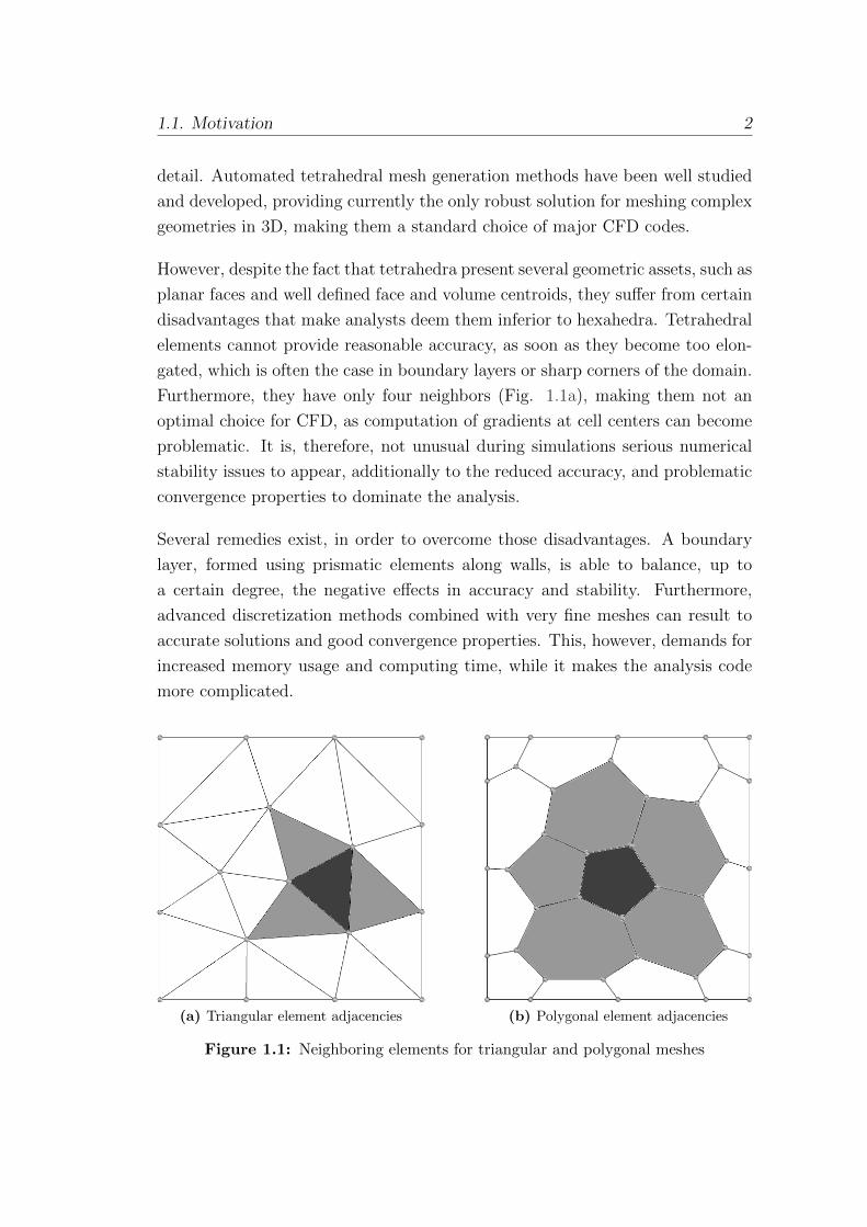
However, despite the fact that tetrahedra present several geometric assets, such as
planar faces and well defined face and volume centroids, they suffer from certain
disadvantages that make analysts deem them inferior to hexahedra. Tetrahedral
elements cannot provide reasonable accuracy, as soon as they become too elon-
gated, which is often the case in boundary layers or sharp corners of the domain.
Furthermore, they have only four neighbors (Fig. 1.1a), making them not an
optimal choice for CFD, as computation of gradients at cell centers can become
problematic. It is, therefore, not unusual during simulations serious numerical
stability issues to appear, additionally to the reduced accuracy, and problematic
convergence properties to dominate the analysis.
Several remedies exist, in order to overcome those disadvantages. A boundary
layer, formed using prismatic elements along walls, is able to balance, up to
a certain degree, the negative effects in accuracy and stability. Furthermore,
advanced discretization methods combined with very fine meshes can result to
accurate solutions and good convergence properties. This, however, demands for
increased memory usage and computing time, while it makes the analysis code
more complicated.
(a) Triangular element adjacencies (b) Polygonal element adjacencies
Figure 1.1: Neighboring elements for triangular and polygonal meshes
1.1. Motivation 3
Recently, an alternative option to tetrahedral meshes has emerged, suggesting
the use of polyhedral elements instead [22, 10]. Polyhedra offer the same level of
automatic mesh generation as tetrahedra do, while they are able to overcome the
disadvantages adherent to tetrahedral meshes. A major advantage of polyhedra
occurs from the fact that they are bounded by many neighbors (Fig. 1.1b),
making approximation of gradients much better that tetrahedra. Furthermore,
they are much less sensitive to stretching and, since their typically irregular
shape is not a restriction for several CFD codes, they offer the possibility of
post-processing and optimization without the strict geometric criteria that are
necessary for optimizing tetrahedral, or even hexahedral meshes.
On the negative side, polyhedra are usually of much more complex geometry
than regular solids, and, depending on the generation method, it cannot always
be guaranteed that they are convex, or, even more, that their faces are planar.
The topology of polyhedral meshes is, typically, also complex, preventing the
implementation of efficient and easy to maintain generation algorithms from
being straightforward. As a further consequence, polyhedral meshes require a
considerable amount of adjacency relations, in comparison to tetrahedral and
hexahedral meshes, making them candidates for resource expensive solutions.
All the above set the basis for an interesting field of exploration in volume mesh-
ing. Previous studies on the subject have shown promising results, however poly-
hedral meshing is still far from becoming a standard practice in CFD simulations.
Some explanations for this may be its limited adoption from analysis codes and
the fact that polyhedra are not an appropriate solution for every type of analysis,
preventing, thus, researches not interested in fluid simulations from being moti-
vated in further investing on the topic. It should be mentioned that, currently,
polyhedral meshes attract more attention in fields such as Computer Graphics
and Medical Imaging, wherein 3D volume rendering is of specific interest. How-
ever, the few researches dedicated to exploring polyhedral mesh generation for
CFD remain active, making constant progress towards more efficient methods
and high quality meshes.
Herein, an overview of the current status of polyhedral mesh generation is at-
tempted, presenting the achievements so far and what is to be expected in the
near future. Additionally, an inquiry into polyhedral mesh generation methods
has been made with the aid of a mesh generation code that was developed, within

1.2. Basic Concepts 4
the scope of this study. A presentation of the basic implementation principles
that were followed is made, with the hope to motivate further development on
the subject. Finally, the results of a set of elementary CFD simulations are dis-
cussed, which have been made possible with the use of DOLFYN CFD code [3]
and SOFiSTiK FEA software [1], in order to assess the performance of the im-
plemented mesh generator, as well as to obtain a first evaluation of the analysis
characteristics of polyhedral meshes.
1.2 Basic Concepts
1.2.1 Voronoi Tessellations
In the past years, the main focus, regarding polyhedral mesh generation, has
been placed on generating Voronoi tessellations. These are structures consisting
of partitions that correspond to a set of generator points, such that every location
within a subdivision is closer to its generator than to any other. Voronoi tes-
sellations are unbounded, with outer partitions extending to infinity. However,
for the purpose of mesh generation, partitions on the exterior are truncated by
the domain’s boundary, forming, this way, a general polyhedral mesh (Fig. 1.2)
[37, 10].
Despite their simple concept, direct generation of 3D Voronoi meshes, to be
used within numerical simulations, is not always straightforward. One way to
retrieve a Voronoi mesh is by applying half-plane intersections, which is, however,
computationally expensive, with a complexity of O(n2 log n) [4]. Another way
is using Fortune’s plane sweep algorithm, which, while of reduced complexity
O(n log n) [4], its implementation for 3D space is considered rather complicated
[10]. Furthermore, an additional obstacle to overcome, which applies in every
mesh generation algorithm, is considering topology in 3D space itself, even when,
conceptually, a method is well defined. Currently, it cannot be claimed that an
efficient direct polyhedral mesh generation method exists, or a robust enough to
be used in CFD simulations.

1.2. Basic Concepts 5
Figure 1.2: Bounded mesh formed by a Voronoi tessellation
1.2.2 Mesh Duality
A different approach in generating polyhedral meshes, which does not suffer by
the aforementioned restrictions, comes with the introduction of indirect mesh
generation methods. These are based on the principle of duality transforms,
which define a mapping from entities of an input mesh, which is referred to as
primal, to a destination mesh, referred to as dual. The main mapping process
dictates that the vertices of a dual mesh are generated at the centers of the primal
cells [17]. This relation is unique, leading to a one-to-one correspondence of the
two counterpart meshes, while it is also characterized by inverse applicability.
This means that the original primal mesh can be obtained back, if the same
mapping is applied to the dual mesh.
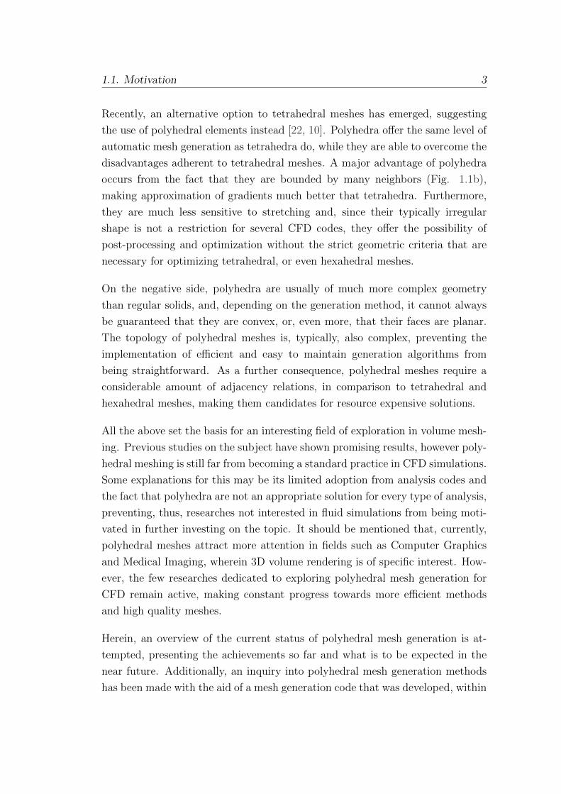
This property can be applied for Voronoi tessellations, as well. The dual coun-
terpart of a Voronoi mesh is a Delaunay triangulation, which is defined as a
partitioning scheme, such that no vertex is inside the circumcircle of any triangle
(Fig. 1.3). The implementation of Delaunay triangulation algorithms is rela-
tively simple and can be of complexity O(n log n), following Ruppert’s algorithm
[11]. As the duality property can be applied both ways, it is then possible to ob-
tain a Voronoi mesh, by applying a duality transform on a previously generated
1.2. Basic Concepts 6
Figure 1.3: Mesh formed by a Delaunay triangulation
Delaunay triangulation, considering the circumcenters of the primal tetrahedra
as generator vertices.
In 3D space, an equivalent mesh generation method would require a tetrahedral
primal mesh that complies with the Delaunay criterion. Delaunay partitioning
is known to maximize the minimum angle of all formed simplices, which leads to
well conditioned tetrahedra. However, in order to obtain a valid dual mesh, a far
stricter criterion needs to be fulfilled: that of well centered tetrahedra, meaning
that the circumcenter of a primal cell needs to be located within its volume [10].
This is something that is not always possible, as tetrahedra at the boundaries
may be very flat, having their circumcenters outside the model’s domain, while
the Delaunay criterion still remains fulfilled. Situations like this are especially
encountered at sharp concavities of the geometric model, and several suggestions
have been made in order to overcome this issue.
Extending the previous concepts, it should be noted that, even though Voronoi
meshes are characterized by desirable numerical properties, a valid polyhedral
mesh does not necessarily have to be one. Except for the boundaries, where cells
are “forced” to conform to the model’s geometry, non Voronoi polyhedra may
exist in the interior as well. Hence, duality transforms do not have to be restricted
to using exclusively primal meshes that are based on the Delaunay criterion.
Other possibilities include non-Delaunay tetrahedral meshes, hexahedral or even
mixed meshes, which are further discussed in chapter (Ch. 3).
1.3. Previous Work 7
Finally, the advantage of indirect mesh generation lies in the fact that efficient
algorithms can be implemented in order to obtain topologically involved dual
meshes, based on primal meshes with simple topology. Furthermore, the primal
meshes, themselves, can be created following equally efficient and well-studied
algorithms. This approach leads into an effective two-step mesh generation,
rather than an expensive, direct one.
1.3 Previous Work
Numerous studies and implementations for the generation of Voronoi tessellations
in 2D exist. However, when it comes to 3D, these are limited and the product
of most cannot be guaranteed to be usable as a mesh for CFD simulations.
The main reason for this emerges by the fact that many researchers focus on
other fields of application, of which most notable is that of Computer Graphics.
It is, nonetheless, worth mentioning some of them, not only for the sake of
completeness, but mostly because the have been studied as a first step towards
polyhedral meshing for simulations in engineering.
Qhull [24] Voronoi mesh generator has been used for many years to produce high
quality 3D tessellations. However, its lack of support for non-convex domains
make it difficult to use for structures of complex geometry. On the other hand,
Voro++ [36], despite its flexibility in generating Voronoi partitions around gen-
erator points, it does not guarantee a fully connected mesh. Finally, Tetgen
mesh generator [31] produces boundary conforming Voronoi partitions as duals
of Delaunay tetrahedral meshes, however the issue of strictly conforming to sharp
concavities seems, so far, not to be treated properly.
All the previous have been open source projects which focus primarily on compu-
tational geometry concepts. Regarding more engineering oriented implementa-
tions, OpenFOAM [20] is an open source CFD software package that has evolved
to a multi-physics tool suitable for numerous types of simulation [13]. One of
its available modules provides the functionality of generating polyhedral meshes,
suitable to be used within the environment of OpenFOAM. Moving to commer-
cial platforms, there are a few that embed OpenFOAM mesh generation, and not
only, procedures into their own functionality. However, probably the first and

1.4. Background Theory 8
most notable, so far, commercial implementation, is that of STAR-CCM+ [29],
developed by CD-adapco, an early adopter of polyhedral meshes as a standard
practice within their software.
Last but not least, through recent publications, automatic polyhedral mesh gen-
eration has received more attention [19, 10]. Garimella et al. are currently fo-
cusing their efforts towards a detailed description of polyhedral mesh generation
methods [10]. Although their code has not, yet, been released, their contribu-
tion through publications has clarified the concepts of generating and optimizing
polyhedral meshes, while ongoing research is being conducted for more advanced
topics. Given the attention that polyhedral meshes have drawn during the past
few years, more concepts and robust implementations are expected in the near
future.
1.4 Background Theory
CFD is based on solving conservation equations for variables relevant to a fluid
flow. These take into consideration sources and sinks, as well as the transport
of material throughout the domain. Common variables of interest include mass,
velocity, pressure, momentum, turbulent kinetic energy, turbulent energy dissi-
pation rate etc.
The integral form of the generic conservation equation of a scalar variable φ takes
the form of (Eq. 1.1) [6]:
∂
∂t
∫Ω
ρφ dΩ +
∫S
ρφv · n dS =
∫S
Γgradφ · n dS +
∫Ω
qφ dΩ (1.1)
where t stands for time, ρ for the fluid density, v for the flow velocity, n for
the unit normal vector of the surface S enclosing a Control Volume (CV) and
Ω for the volume occupied by the CV. Γ is the diffusivity of quantity φ and qφ
represents the sources or sinks of φ.
Setting φ = 1 and assuming no internal sources or sinks, the mass conservation
equation occurs, in its integral form, which establishes the continuity of the

1.4. Background Theory 9
Control Volume (Eq. 1.2):
∂
∂t
∫Ω
ρ dΩ +
∫S
ρv · n dS = 0 (1.2)
In a similar manner, for a fixed volume in space, the momentum conservation
equation is formed by setting φ = v (Eq. 1.3):
∂
∂t
∫Ω
ρv dΩ +
∫S
ρvv · n dS =∑
f (1.3)
where∑
f represents the forces that act on the fluid contained in the volume.
These can be surface forces, such as pressure, surface tension, etc., or body forces,
such as gravity.
The application of these conservation equations is performed within the context
of a method of discretization. There are various ways to formulate a solution
scheme for CFD analysis. Historically, the oldest approach has been the Finite
Difference Method. Despite being the simplest available, its restricted applica-
tion to structured grids makes this method of little use for modern analysis of
complex structures. Additionally, special care is required in order to apply the
conservation principles on coarse grids, raising further restrains in commonly
using a Finite Difference approach.
Another discretization scheme that can be used for CFD is the Finite Element
Method. The advantage of FEM relies on the fact that arbitrary geometries can
be easily handled and, with a robust mathematical background, many categories
of CFD problems can be treated. It is ideal for diffusion dominated simulations,
as well as viscous, free surface problems. However, it can be very slow for large
problems, while it is not well suited for the analysis of turbulent flow.
The preferred approach of most CFD codes is that of the Finite Volume Method
(FVM). In this method, the domain is subdivided into Control Volumes, to which
the conservation equations are individually applied. Computations take place at
the centroid of each Control Volume, where a value for the variable of interest is
computed. The conservation equation, as applied in its integral form, becomes
then (Eq. 1.4):

1.4. Background Theory 10
∫S
ρφv · n dS =
∫s
Γgradφ · n dS +
∫Ω
qφ dΩ (1.4)
It should be mentioned, that the conservation equation is transformed from a
volume to a boundary integral, whereas the sum of mass and impulse passing
through the surface of the control volume, minus the contribution of any existing
sources or sinks, must be zero [16].
The main advantage of FVM is that it is suitable for every type of grid, with-
out limiting the cell shape, while the conservation equations are fulfilled even
on coarse grids [2]. The simplicity of the method makes easy its algorithmic
implementation, with well-developed iterative solvers guaranteeing its efficiency.
However, one disadvantage of FVM is that it is not well-suited for higher order
analysis. Finally, the fact that FVM is not restricted to using cells of specific
shape is exactly the property that enables the use of polyhedral meshes.
11
Chapter 2
Mesh Topology and
Representation
2.1 Introduction
The discretization of a continuum to a mesh model, which adheres to a respect-
ful description of the geometry, is one of the most expensive steps in modern
computational mechanics. A continuous effort is being made by researchers, in
order minimize the storage and computing resources that are required during
mesh generation. Furthermore, the structure of the mesh database that is used
has a significant influence on performance, during the following steps of analysis
and post-processing. Taking into consideration the way in which mesh entities
need to be stored and, therefore, accessed, is not a trivial task and, in many
cases, there is no straightforward answer as to what the optimum representation
scheme is for a specific application. In most cases, demands in storage on the
one hand, and efficiency on the other act in an competitive way, raising a ques-
tion of minimizing storage requirements without sacrificing performance. In the
following paragraphs, an attempt is made to present the basic concepts in mesh
topology and clarify the needs of polyhedral mesh generation, regarding mesh
data structures.
2.2. Definitions 12
2.2 Definitions
2.2.1 Topological Entities
The topology of a mesh is an abstraction of the geometric model, that provides
unambiguous, shape independent information about the relation between the
entities that form the mesh structure. To this end, a mesh database is used in
order to store various-level attributes of entities of different dimensions [7]. These
typically include 0D entities, referred to, in literature, as vertices or nodes, 1D
entities, referred to as edges, 2D entities, referred to as faces or facets and 3D
entities, referred to as solids, volumes, regions or cells. In this study, the terms
vertex, edge, face and solid are preferred.
2.2.2 Adjacent Entities
Each topological entity is bounded by a set of entities of lower dimension, form-
ing a geometric object. Solids are bounded by faces, faces by edges and edges are
bounded by vertices. Apart from this fundamental relation between entities, it is
often useful to acquire a more advanced description of the relative connectivity
that exists between the entities of a mesh structure. Even though in Graph The-
ory a distinction is made between different types of entities’ relations, the term
adjacent entity is uniformly used, in the context of mesh databases, to describe
not only bounding entities but also directly connected neighboring entities of the
same or higher dimension.
However, while for neighboring entities of lower dimension the adjacency relation
unambiguous, connectivity information referring to entities of the same or higher
dimensions may not always be unique. As an example, in a hexahedral mesh, a
solid in the interior of a domain has 6 adjacent faces, 12 adjacent edges and 8
adjacent vertices. However, the adjacent solids of a hexahedron can be considered
to be 6, those sharing common faces with, or 26, those sharing common edges
with. It is, thus, important to define what is regarded as an adjacent entity
within a certain context of use. Herein, connectivity of entities of the same or
higher dimension, whenever needed, is described in a periphrastic way, in order

2.2. Definitions 13
to avoid ambiguously interpreted relations.
2.2.3 Entities Classification
Mesh classification against the geometric domain is defined by the unique associ-
ation of a mesh entity of dimension di, to a geometric model entity of dimension
dj, where di ≤ dj. Information about a mesh entity’s classification allows for con-
sideration of the original geometric model rather than the topological attributes
of the mesh. This way, a direct link to the geometric shape information of the
domain is achieved. A mesh entity is classified on a model entity, if it forms part
or all of the discretization of the model entity [10].
Being able to acquire information about the classification of an entity, enables
mesh generation algorithms to determine which mesh entities form the geometric
model’s boundaries, which lie entirely in the interior or even which are part of
internal boundaries. This distinction of mesh entities yields useful information
about their individual significance in the mesh’s respectful representation of the
geometric model and is essential in order to preserve the model’s boundaries or
other features, such as sharp edges or corners.
The classification of an entity is determined using its topological relation with
adjacent entities of the same or other dimensionality. For three dimensional
meshes, the origin for acquiring classification information about all entities is
the classification of the faces of the mesh structure, which is then inherited by
adjacent entities of lower or higher dimension. This concept is further described
in (Sec. 2.4.3).
2.2.4 Notation
In the following, vertices, edges, faces and solids of a mesh are referred to as
V, E, F, and S, respectively. A set of entities is enclosed within curly brackets
” ” and adjacency relationships are represented by parenthesis ”( )”. As an
example, a face of a solid can be referred to as F(S), while F(S) denotes the
set of faces forming a solid. Finally, an arrow next to an adjacency relationship
2.3. Mesh Representation Schemes 14
Table 2.1: Notation of Adjacency Operators
Entity Type Solid Face Edge VertexSolids of - S(F) ↑ S(E) ↑ S(V) ↑Faces of F(S) ↓ - F(E) ↑ F(V) ↑Edges of E(S) ↓ E(F) ↓ - E(V) ↑Vertices of V(S) ↓ V(F) ↓ V(E) ↓ -
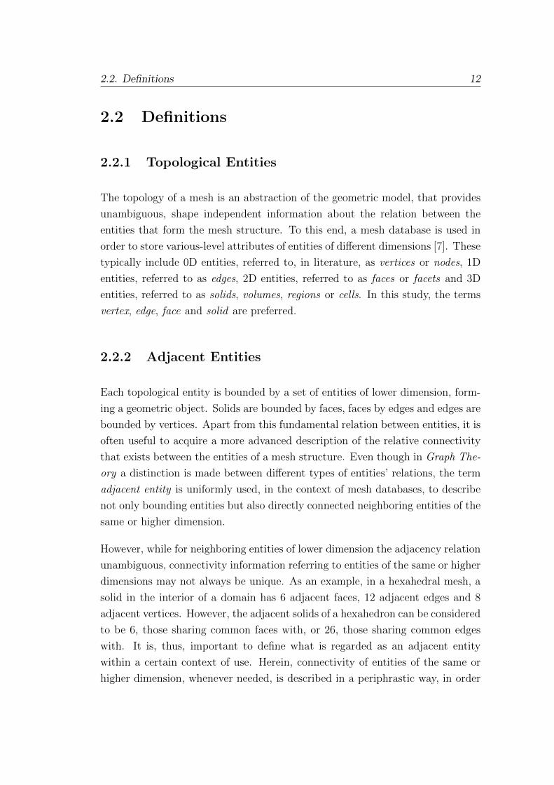
represent whether an upper or lower level entity is being accessed (Tab. 2.1) [7].
2.3 Mesh Representation Schemes
2.3.1 Explicit and Implicit Representation
Data structures that are commonly used to describe meshes can be divided into
two major categories: full and reduced representation schemes. What differen-
tiates the two is whether there exists an explicit way to access every level of
mesh entities, or entities of one or more levels are omitted. Furthermore, for
both categories, various ways may exist to describe the adjacency relationships
between entities of the same or different dimension, providing a flexible way to
access entities according to an application’s demands. An explicit description of
mesh entities of a certain dimension exists in the data structure, when there is
at least one way to directly refer to the mesh entities. These faces can then be
referred to by an index or identity number and iterators may be used to access
the available information.
As an example, a data structure that contains information about the faces that
exist in a 3D mesh is said to provide explicit access to the mesh’s faces. This
information may include the mesh’s edges that form the boundaries of each
face, provided that edges are also explicitly stored. Another possibility could
be storing information about the mesh’s vertices that form each face. There is,
naturally, no restriction in explicitly storing both adjacency descriptions, however
this would mean increased demand in memory, when access to face’s vertices
could have been achieved through the face’s edges, being aware of their starting
and ending vertex. On the other hand, when a certain entity level is omitted,

2.3. Mesh Representation Schemes 15
implicit access to the entities of that dimensionality may be possible. However, in
this case, one would only be able to refer to them as adjacent entities of explicitly
stored entities of a higher or lower level. If, in the previous example, information
about mesh’s edges is not stored in any way, there may be an implicit access to
face’s edges, given the face’s vertices.
It is to be noted that, for every mesh entity of non-zero dimension, there should
always exist an adjacency relationship, or a combination of them, that is able
to explicitly or implicitly describe the entity’s connectivity with mesh vertices.
Although no theoretical restriction applies to describing a plain topological rela-
tionship, this demand emerges from the fact that, in structural modeling practice,
a mesh is not a mere topological entity but a way to represent a corresponding
geometric model. As, in common meshes, the only entities that contain geomet-
ric information are vertices, through their coordinates, it is always required that
higher level entities are able to access vertices’ information, otherwise the mesh
entity would be geometrically undefined.
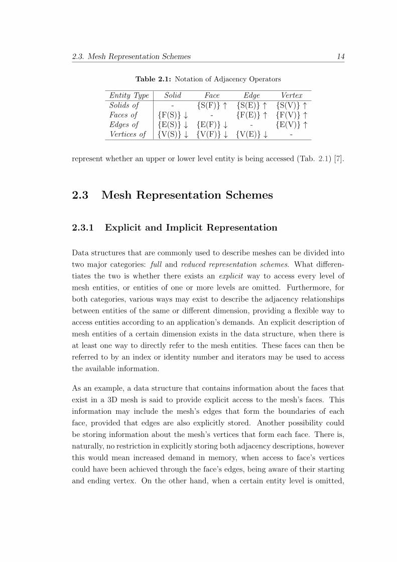
2.3.2 Full Mesh Data Structures
Data structures that explicitly store topological entities of all dimensions, namely
vertices, edges, faces and, for 3D meshes, solids, are referred to as full mesh rep-
resentations. Even though not all connections are always explicitly described, it
is possible to implicitly retrieve adjacency information by combining the existing
connectivity descriptions.
Full data structures require relatively high amount of storage space, compared
to reduced data structures [7]. However, with modern systems specifications,
describing geometric models in a satisfactory level of detail is usually not an
issue, depending on the analysis type. On the other hand, computational effort,
regarding mesh entities’ connectivity, is significantly reduced, giving full mesh
representations a noticeable advantage in performance [7, 8].
2.3. Mesh Representation Schemes 16
(a) F1 (b) F2
Figure 2.1: Common cases of full mesh representation schemes: explicit adjacencyinformation is included for entities of all dimensions
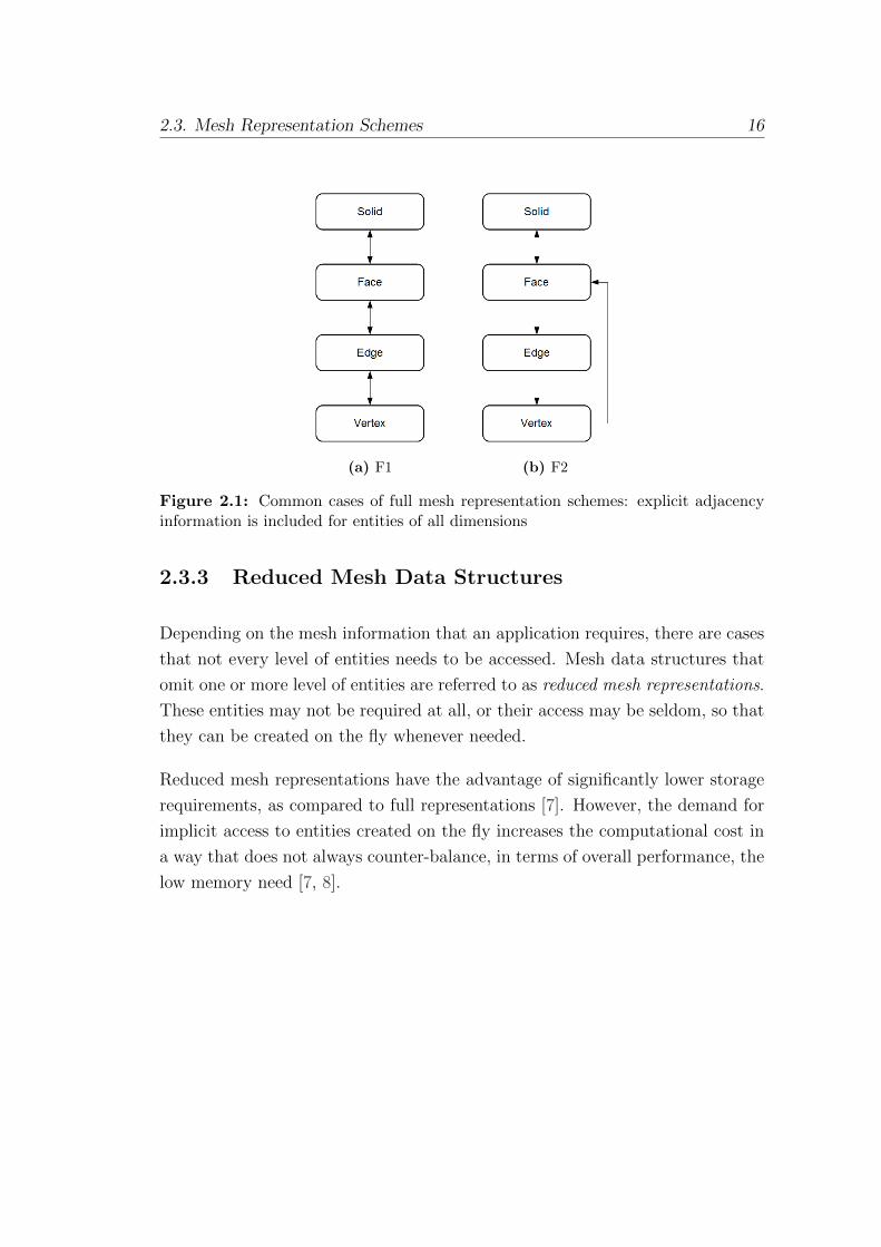
2.3.3 Reduced Mesh Data Structures
Depending on the mesh information that an application requires, there are cases
that not every level of entities needs to be accessed. Mesh data structures that
omit one or more level of entities are referred to as reduced mesh representations.
These entities may not be required at all, or their access may be seldom, so that
they can be created on the fly whenever needed.
Reduced mesh representations have the advantage of significantly lower storage
requirements, as compared to full representations [7]. However, the demand for
implicit access to entities created on the fly increases the computational cost in
a way that does not always counter-balance, in terms of overall performance, the
low memory need [7, 8].
2.4. Representation of Polyhedral Meshes 17
(a) R1 (b) R2
Figure 2.2: Common cases of reduced mesh representation schemes: adjacency in-formation for implicitly represented entities is noted in dashed objects
2.4 Representation of Polyhedral Meshes
2.4.1 Data Structures
An important characteristic that a mesh data structure should have, is being
able to effectively provide the necessary information required by the procedures
that create and / or use that data. These needs can be different for various ap-
plications and are dictated by the information requests, made within the context
of use.
One major problem with the commonly used element-vertex mesh data struc-
tures, is the lack of information relating the mesh entities to regions of the
corresponding geometric model that are of special interest . More specifically,
they provide insufficient information regarding the classification of primal mesh
entities, which is of a decisive role during dual mesh generation. Furthermore,
such representations are only functional with the aid of template-elements, that
describe the relative position of a vertex within the element (Fig.2.3). It is ap-
parent that for cells of arbitrary shape this cannot apply.
During polyhedral mesh generation, explicit access to mesh entities of all dimen-

2.4. Representation of Polyhedral Meshes 18
(a) Hexahedral element template (b) Tetrahedral element tem-plate
Figure 2.3: Element adjacency templates
sions is required, as is described in detail in chapter (Ch. 3). Therefore, a full
mesh data structure is needed, which allows for complete and fast access to mesh
entities’ adjacency relationship. The only restriction that applies, when selecting
among different full representation options, is that solids must be explicitly aware
of their faces, or, in other words, the relationship F(S) that corresponds to the
polygons that form a polyhedron cannot be described in an implicit way. The
reason behind this restriction is that polyhedral shapes are, in general, arbitrary,
with solids of the same mesh having different numbers of faces. What is more, the
polygonal faces themselves have varying numbers of edges and vertices. Thus, it
is not possible to establish E(S) or V(S) relationships in a predefined way
throughout the mesh, as opposed to meshes of elements with pre-defined shape.
In a pure hexahedral or tetrahedral mesh, for example, an explicit V(S) ad-
jacency description would be possible, by storing the vertices of each element
in locally consistent positions (Fig. 2.3a, 2.3b). By forming such a pre-defined
V(S) template, all other adjacency relations is possible to be derived on the
fly.
As far as polygonal faces are concerned, even though E(F) and V(F) ad-
jacency relationships cannot be locally predefined as well, the fact that faces
are required to have a counter-clockwise orientation guarantees that it is always
possible to access a face’s edges or vertices in the correct order, knowing which
entity is at which relative position.
2.4. Representation of Polyhedral Meshes 19
Finally, the most often requested adjacency relationships refer to entities of one
or two levels apart and, thus, it makes sense to explicitly describe them. Two
well qualified candidates are, therefore, the mesh representations depicted in
(Fig. 2.1a, 2.1b), from which the former has been chosen, within the scope of
the present work, due to it’s simpler design and the more intuitive hierarchical
order.
Therefore, a mesh database, herein, explicitly contains entries for existing vertices
and their coordinates, edges defined by their bounding vertices, faces defined by
their bounding edges and solids defined by their bounding faces. Additionally,
a face is aware of the solids it is adjacent to, an edge is aware of the faces it
is adjacent to and a vertex is aware of the edges it is adjacent to. Every other
connectivity relation is implicitly retrieved by making use of the above, explicitly
stored information.
2.4.2 Adjacent Entities Orientation
It is common for mesh entities of certain dimensions to be defined in a way that
describes their orientation in space. For example, when faces stored in a mesh
database, it is done so in an ordered manner, meaning that the edges and vertices
that describe them are accessed in a counter-clockwise sequence that denotes
a positive definition of the faces’ orientation. It is also of common practice
that each solid within a mesh is bounded by 2D entities that are always facing
outwards, or that they are positively oriented with respect to the solid. These
are conventions that allows for a unified consideration of the relative definition
between adjacent entities.
Therefore, when a face is accessed as an adjacent entity of a solid, it is necessary
to know if the counter-clockwise definition of the face coincides with the definition
that denotes a positive orientation with respect to the solid it bounds. If this is
the case, then the adjacent face is marked as positively oriented, usually setting
a +1 flag in the solid-face adjacency information. Otherwise, it is negatively
defined and a -1 flag is set, which will be considered to access, from the solid’s
perspective, the adjacent face’s edges or vertices in the opposite sequence that
the face is defined within the mesh structure database.

2.4. Representation of Polyhedral Meshes 20
Similarly, edges are usually stored, knowing their starting and ending vertices.
For a face to properly access the vertices of one of its adjacent edges, it needs
to be aware of whether the orientation of the edge, as stored in the database, is
respectful to the counter-clockwise that the face should have, or if it is oriented
the opposite way. A +1 / -1 flag is then stored for respective face-edge adjacency
information.
Finally, the same applies for the vertices of the mesh, where a +1 flag is noted
for an adjacent edge of which the vertex is its starting point, and a -1 for an
adjacent edge that uses this vertex as an ending point. However, in this case,
this relation of orientations can be dynamically retrieved, by the information
stored in the edge, and no flag needs to be stored on the vertex side.
2.4.3 Boundary Detection
Although solids cannot be classified on a boundary surface, as they are always in
the interior of the model, those solids whose at least one adjacent face is classified
on the boundary can be detected by iterating through their faces. These solids
form the boundary layer of the geometric model, which is of special interest in
CFD simulations, thus it is often useful to be able to detect them.
A face is said to be classified on the boundary of the geometric model, when it is
adjacent to only one solid, which means that the “free” side of the face forms an
external boundary. In the opposite case, where a face is adjacent to two solids,
it is classified in the interior of the geometric model. Additionally, it is common
in mesh generation to assign specific attributes to faces classified on the same
model boundary surface, referring to them under the same boundary identifier,
usually group number. This way, it is topologically possible to access mesh faces
that form a common model boundary and distinguish them from faces on other
boundaries.
Mesh edges inherit their classification by their adjacent faces. Specifically, when
an edge has at least one adjacent face that is classified on a model’s boundary
surface, the edge is also classified on the same boundary. To be more precise,
in a conforming non-manifold three-dimensional mesh, an edge will have either
zero or at least two adjacent boundary faces, however detecting one of them can
2.4. Representation of Polyhedral Meshes 21
be considered enough to classify the edge on the boundary as well.
Furthermore, when an edge’s adjacent boundary faces are classified on different
boundary surfaces of the model, this denotes the edge’s classification on a model’s
boundary edge, where two of its boundary surfaces intersect. It is, therefore,
adequate to count the amount of different boundary identifiers that are assigned
to the adjacent faces of an edge, in order to conclude whether this edge is internal
(zero boundary identifiers), on a boundary surface (one identifier), on a boundary
edge (two identifiers), or is a non-manifold edge (more than two identifiers).
Extending the aforementioned classification criteria for vertices, a mesh vertex is
classified on a model’s boundary surface, when at least one of its adjacent edges
is also classified on a boundary surface. Additionally, when at least one of the
adjacent edges of a vertex is classified on a model’s boundary edge, then the
vertex is also classified on the same boundary edge. Finally, when there exist
at least two adjacent edges classified on two different model’s boundary edges,
the vertex is classified on a model’s corner, formed at the intersection of the
boundary edges.
In other words, the classification of a vertex with respect to the model can be
determined by counting the amount of different boundary identifiers assigned to
the adjacent faces of the vertex. Zero boundary identifiers denote an internal
vertex, while vertices on a boundary surface have adjacent faces with a unique
identifier. Nodes on model’s boundary edges have adjacency relationships to
faces of two boundary identifiers in total and vertices on a model’s corner sum
up with three adjacent boundary identifiers. Finally, when a vertex has adjacent
faces classified to more than three different boundary surfaces, the vertex is non-
manifold.
2.4.4 Significant Entities
In the previous chapter (Ch. 1), an overview of the principles behind polyhe-
dral mesh generation was given, where the distinction was made between primal
entities that contribute to the generation of dual vertices. All types of primal
entities, depending on their classification, participate in forming dual entities,
and affect the topological connectivity of the obtained mesh. However, those

2.4. Representation of Polyhedral Meshes 22
primal entities that participate in the generation of dual vertices are of special
interest, as they form the main contributors to the definition of the geometry of
the dual mesh. This comes as a consequence of the fact that dual vertices will be
the only dual entities that will contain geometric information: their coordinates.
This distinction is made by defining the criteria under which a primal mesh entity
is considered to have important geometric properties that need to be preserved in
the dual mesh. In this context, they are referred to as significant primal entities.
These can be of any dimension and classification, however they are distinguished
by certain combinations of characteristics that make them special. Usually, they
are classified on the geometric model’s boundaries or boundary intersections and
they contribute a central point within their local domain, that becomes a dual
vertex. However, it is up to the user to determine the exact criteria that will
form the vertices of a dual mesh, allowing, this way, for flexibility over the mesh
generation.
Primal solids are always regarded as significant and each contributes a dual vertex
in a central point within its volume. Their union represents the domain of the
geometric model and they are the generators of all dual vertices that will lie in
the interior of the dual mesh, once the polyhedral mesh generation is complete.
Significant primal faces are those that are classified on the geometric model’s
boundary surfaces, and can be detected as described in (Sec. 2.4.3). Each
significant face contributes a dual vertex lying on a central point within its area.
The resulting vertices are classified on the model’s boundaries as well, and are
those that will define the boundary surfaces’ geometry for the polyhedral mesh.
The primal edges, the geometry of which needs to be preserved in the dual mesh,
are those that are classified on the boundary edges of the geometric model or, in
other words, on the boundary surfaces’ intersections. They constitute a subset of
the edges classified on the boundary, that are connected to two or more significant
faces that belong to different boundary surfaces. Except for the fundamental
topological criteria, geometric criteria may apply as well. A common practice
is to mark a primal edge as significant, when two of its adjacent significant or
boundary faces form an angle that is smaller than a predefined value, regardless
of the surface they are classified on. Depending on the implementation and the
analysis prerequisites, more geometric criteria may apply.

2.4. Representation of Polyhedral Meshes 23
Finally, significant primal vertices are those that are classified on the geometric
model’s corners or, in other words, lie on significant edges’ intersections, when
these edges are connected, in total, to three or more different boundary surfaces.
This is something that can be detected as in the previous case, of significant
edges. Significant vertices contribute an exact copy of themselves to the polyhe-
dral mesh, and their role is to preserve the model’s corner. In a similar way as
with significant edges, additional geometric criteria may apply, as well, for the
detection of significant vertices. A common case considers primal vertices that
are connected to significant or boundary edges that form an angle that is smaller
than a predefined value.

24
Chapter 3
Polyhedral Mesh Generation
3.1 Introduction
One thing to consider, when it comes to mesh generation, is the distance that
often exists between the mathematical description of a method and its algorith-
mic implementation for a specific field of application. This has also been the
case with polyhedral mesh generation, which, despite the existence of thorough
research, regarding its fundamental principles, it has yet to become a common
choice of analysts in CFD simulation. One important factor for this is the lack
of a broad selection of polyhedral mesh generators that analysts could choose
from, as challenges regarding the implementation of such tools, suitable for CFD
analysis, still exist. Recently, an attempt to publicly address current issues in
generating polyhedral meshes has been made, suggesting a robust methodology
in mesh generation [10]. Having this progress in mind, an independent study in
polyhedral meshing has been made in the present work, which has resulted to the
implementation of a polyhedral mesh generator. The basic steps that have been
followed, as well as the challenges that have been encountered, are described in
the following paragraphs.
3.2. Methodology 25
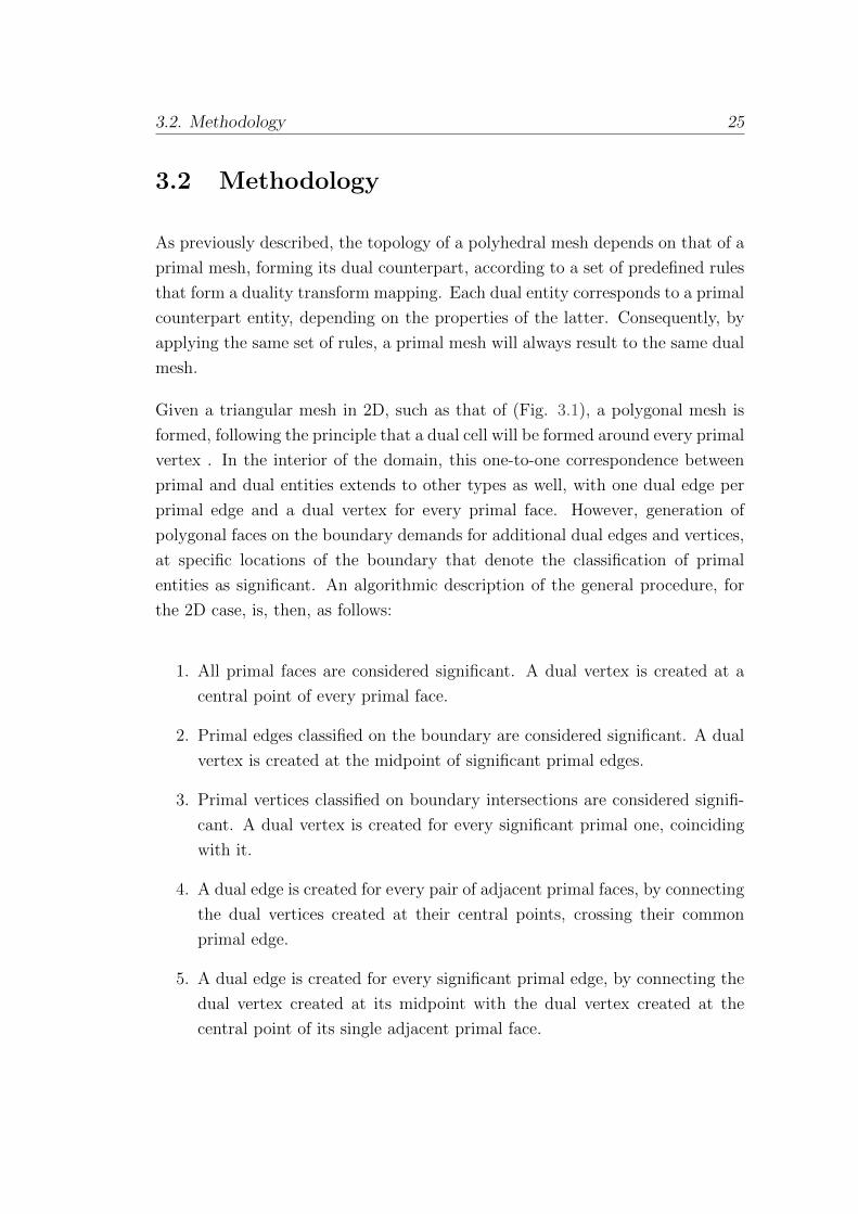
3.2 Methodology
As previously described, the topology of a polyhedral mesh depends on that of a
primal mesh, forming its dual counterpart, according to a set of predefined rules
that form a duality transform mapping. Each dual entity corresponds to a primal
counterpart entity, depending on the properties of the latter. Consequently, by
applying the same set of rules, a primal mesh will always result to the same dual
mesh.
Given a triangular mesh in 2D, such as that of (Fig. 3.1), a polygonal mesh is
formed, following the principle that a dual cell will be formed around every primal
vertex . In the interior of the domain, this one-to-one correspondence between
primal and dual entities extends to other types as well, with one dual edge per
primal edge and a dual vertex for every primal face. However, generation of
polygonal faces on the boundary demands for additional dual edges and vertices,
at specific locations of the boundary that denote the classification of primal
entities as significant. An algorithmic description of the general procedure, for
the 2D case, is, then, as follows:
1. All primal faces are considered significant. A dual vertex is created at a
central point of every primal face.
2. Primal edges classified on the boundary are considered significant. A dual
vertex is created at the midpoint of significant primal edges.
3. Primal vertices classified on boundary intersections are considered signifi-
cant. A dual vertex is created for every significant primal one, coinciding
with it.
4. A dual edge is created for every pair of adjacent primal faces, by connecting
the dual vertices created at their central points, crossing their common
primal edge.
5. A dual edge is created for every significant primal edge, by connecting the
dual vertex created at its midpoint with the dual vertex created at the
central point of its single adjacent primal face.
3.2. Methodology 26
Figure 3.1: A primal triangular mesh and its general polygonal dual
6. A dual edge is created for every pair of adjacent significant primal edges
classified on the same boundary, by connecting the dual vertices created at
their midpoints.
7. A dual edge is created for every significant primal edge classified on a
boundary intersection, forming a corner of the geometric model, by con-
necting the dual vertex created at its midpoint with the dual vertex on the
boundary intersection.
8. A dual face is created for every primal vertex, by collecting the dual edges
that connect the dual vertices, which correspond to the adjacent faces of
the primal vertex (generated in step 4).
9. If the generator primal vertex is classified on a boundary or a boundary
intersection, the dual edges classified on the same boundary are additionally
considered, in forming the dual face (generated in steps 5 – 7).
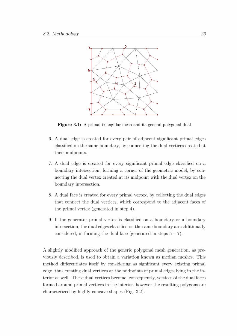
A slightly modified approach of the generic polygonal mesh generation, as pre-
viously described, is used to obtain a variation known as median meshes. This
method differentiates itself by considering as significant every existing primal
edge, thus creating dual vertices at the midpoints of primal edges lying in the in-
terior as well. These dual vertices become, consequently, vertices of the dual faces
formed around primal vertices in the interior, however the resulting polygons are
characterized by highly concave shapes (Fig. 3.2).
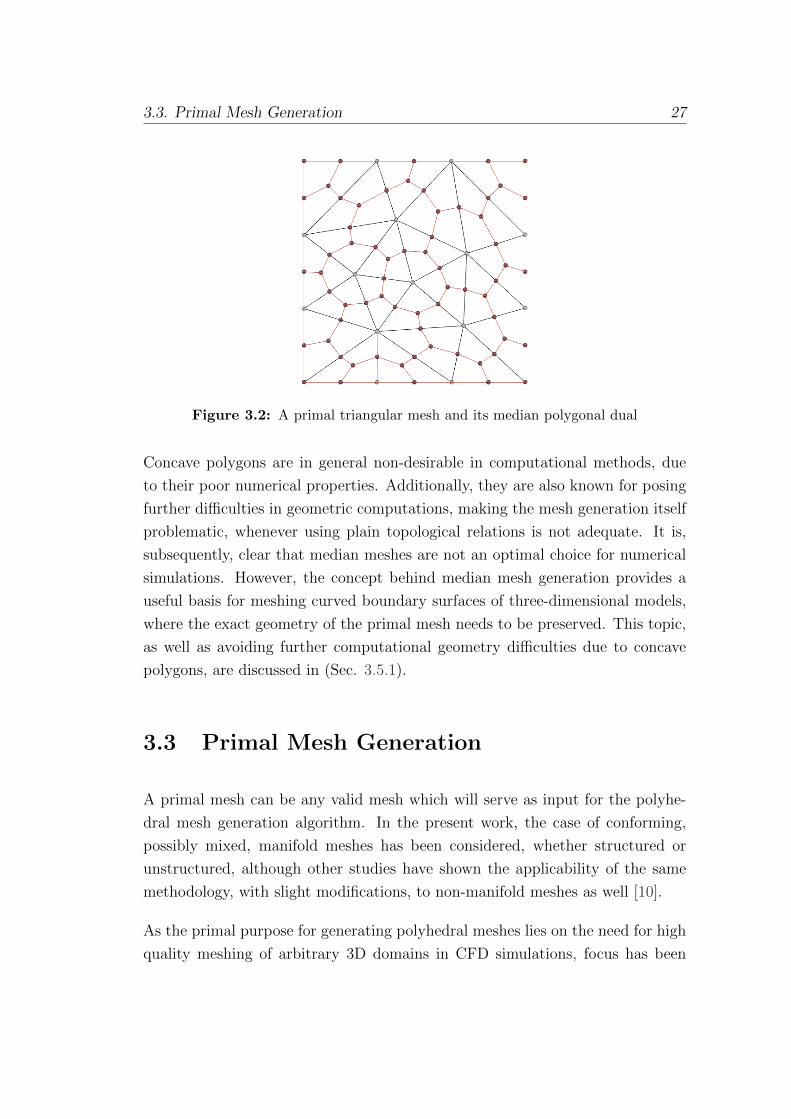
3.3. Primal Mesh Generation 27
Figure 3.2: A primal triangular mesh and its median polygonal dual
Concave polygons are in general non-desirable in computational methods, due
to their poor numerical properties. Additionally, they are also known for posing
further difficulties in geometric computations, making the mesh generation itself
problematic, whenever using plain topological relations is not adequate. It is,
subsequently, clear that median meshes are not an optimal choice for numerical
simulations. However, the concept behind median mesh generation provides a
useful basis for meshing curved boundary surfaces of three-dimensional models,
where the exact geometry of the primal mesh needs to be preserved. This topic,
as well as avoiding further computational geometry difficulties due to concave
polygons, are discussed in (Sec. 3.5.1).
3.3 Primal Mesh Generation
A primal mesh can be any valid mesh which will serve as input for the polyhe-
dral mesh generation algorithm. In the present work, the case of conforming,
possibly mixed, manifold meshes has been considered, whether structured or
unstructured, although other studies have shown the applicability of the same
methodology, with slight modifications, to non-manifold meshes as well [10].
As the primal purpose for generating polyhedral meshes lies on the need for high
quality meshing of arbitrary 3D domains in CFD simulations, focus has been

3.4. Dual Mesh Generation 28
placed on tetrahedral primal meshes, which are flexible in representing complex
geometries. Given the fact that the quality of the input mesh influences directly
the output, a high quality tetrahedral mesh generator is a prerequisite towards
polyhedral meshing. Furthermore, in order to obtain characteristics as close as
possible to a Voronoi tessellation, even though it is not possible to achieve an
exact meshing of such kind, a mesh generator capable of deriving a Delaunay
tetrahedralization is preferred.
Generating a qualified primal mesh, suitable to form a basis for deriving a poly-
hedral dual mesh, does not require any method that the modern analyst is not
familiar with. Already available mesh generation tools are capable of delivering
high quality meshes. To this end, in the present work, NETGEN mesh generator
has been used for generating tetrahedral primal meshes [18] [27].
3.4 Dual Mesh Generation
Dual meshes are generated in a hierarchical order, starting from 0D up to 3D
entities, given criteria that emerge from primal entities classification. The fun-
damental concept, as an extension to the two-dimensional case, is to create dual
volumes around every vertex of the primal mesh, establishing this way a one-to-
one correspondence between them. The way to obtain dual entities is described
in details in the following paragraphs.
3.4.1 Dual Vertices
Every cell of the primal mesh, whether classified on the boundary or in the inte-
rior, is considered a significant entity, resulting to a corresponding dual vertex,
created at a central point of the primal volume. Common choices where dual
vertices can be positioned are primal volumes’ centroids or, in the case of tetrahe-
dra, their circumcenters are an alternative option. The selection of central points
is crucial for the quality of the resulting polyhedral volumes and is discussed in
more detail in (Sec. 4.3.1). Dual vertices in the interior are generated by parsing
through every cell of the primal mesh and computing its central point.

3.4. Dual Mesh Generation 29
Figure 3.3: Generation of internal dual vertices
Every face on the boundary of the primal mesh will be considered during dual
mesh generation by contributing its central point. As is also the case with central
points of volumes, the selection of central points of boundary faces has a decisive
effect on the shapes of the dual polygons that will be formed on the boundary.
Common central points are primal faces’ centroids or, in the case of triangles,
their circumcenters can be also used. Dual vertices of this classification are gen-
erated by parsing through every primal face of the source mesh and considering
those classified on the model’s boundary. This is achieved by evaluating if a face
is connected to one, and only one, primal volume.
Primal edges on a boundary edge of the model contribute their midpoints in order
to form dual vertices. These dual vertices are generated by parsing through every
primal edge and considering those classified on a model’s boundary edge. This
is achieved by evaluating if two of their adjacent primal faces are classified on
two different boundaries of the model.
Finally, dual vertices are created coinciding with primal vertices at positions
where the model’s boundary edges intersect, forming “corners” of the model.
These vertices are generated by parsing through every primal vertex and consid-
ering those classified on a model’s boundary edge intersection. This is achieved
by evaluating if at least two of their adjacent primal edges are classified on differ-
ent boundary edges of the model, which is, in turn, evaluated by verifying that
3.4. Dual Mesh Generation 30
the edges’ adjacent faces, in total, are classified on at least 3 boundary faces of
the model.
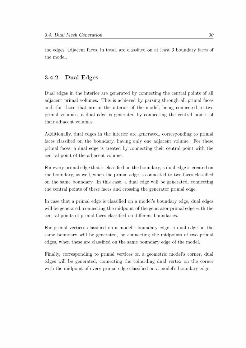
3.4.2 Dual Edges
Dual edges in the interior are generated by connecting the central points of all
adjacent primal volumes. This is achieved by parsing through all primal faces
and, for those that are in the interior of the model, being connected to two
primal volumes, a dual edge is generated by connecting the central points of
their adjacent volumes.
Additionally, dual edges in the interior are generated, corresponding to primal
faces classified on the boundary, having only one adjacent volume. For these
primal faces, a dual edge is created by connecting their central point with the
central point of the adjacent volume.
For every primal edge that is classified on the boundary, a dual edge is created on
the boundary, as well, when the primal edge is connected to two faces classified
on the same boundary. In this case, a dual edge will be generated, connecting
the central points of these faces and crossing the generator primal edge.
In case that a primal edge is classified on a model’s boundary edge, dual edges
will be generated, connecting the midpoint of the generator primal edge with the
central points of primal faces classified on different boundaries.
For primal vertices classified on a model’s boundary edge, a dual edge on the
same boundary will be generated, by connecting the midpoints of two primal
edges, when these are classified on the same boundary edge of the model.
Finally, corresponding to primal vertices on a geometric model’s corner, dual
edges will be generated, connecting the coinciding dual vertex on the corner
with the midpoint of every primal edge classified on a model’s boundary edge.
3.4. Dual Mesh Generation 31
Figure 3.4: Generation of internal dual edges
3.4.3 Dual Faces
Dual faces in the interior are generated by collecting the dual edges that have
been created, by connecting the central points of the primal volumes surrounding
primal edges. This is achieved by parsing through primal edges and, for every
connected primal face, the corresponding dual edge is collected. When all dual
edges surrounding a primal edge have been retrieved, they have to be sorted
according to their vertices, following a counter-clockwise orientation.
For primal vertices classified on a model’s boundary surface, a dual face is gener-
ated, by collecting all the dual edges surrounding a vertex, that are also classified
on the same boundary. These dual edges correspond to primal edges connected
to the primal vertex, that are also classified on the same boundary.
Furthermore, for every primal vertex classified on a model’s boundary edge, a
dual face is generated for every set of connected primal edges that are classified
on the same boundary surface, considering also those classified on the boundary
edge. The dual edges corresponding to each set of primal edges are collected
and sorted around the primal vertex, using as a reference vector the mean of the
normals of the faces classified on the corresponding boundary surface.
Finally, primal vertices classified on the geometric model’s corners, where the

3.4. Dual Mesh Generation 32
Figure 3.5: Generation of internal dual faces
edges of the model intersect, result to the formation of one dual face for every
intersecting boundary surface. Each dual face is formed by collecting the dual
edges that connect the centers of primal faces classified on the same boundary,
as well as the dual edges connecting the same centers with the midpoints of
significant primal edges. Additionally, the dual edges connecting these midpoints
to the dual vertex on the corner are considered, in order to form a closed dual
face.
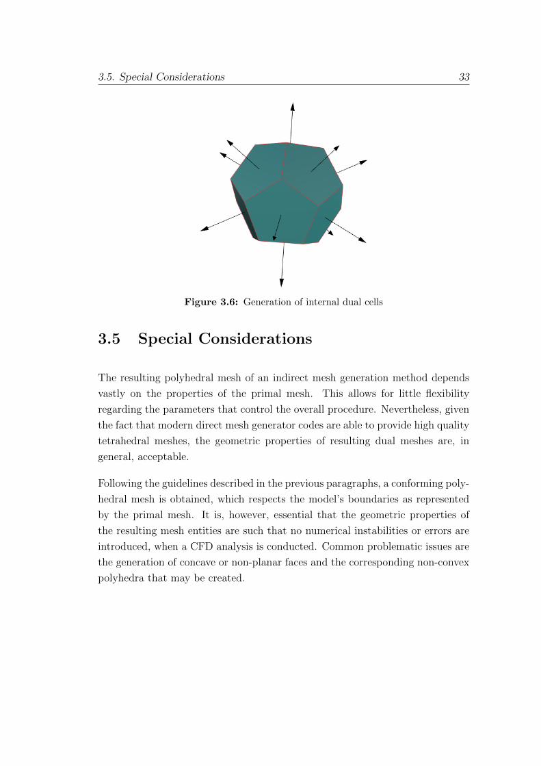
3.4.4 Dual Solids
After dual entities of all lower dimensions have been created, polyhedral volumes
are formed around every vertex of the primal mesh. This is achieved by iterating
through the primal edges connected to each registered primal vertex. The dual
faces, which have previously been generated and correspond to primal edges,
are collected, forming the boundaries of the dual volumes. In the case of primal
vertices on a model’s “corner”, the dual faces corresponding to the primal vertices
are considered as well.
3.5. Special Considerations 33
Figure 3.6: Generation of internal dual cells
3.5 Special Considerations
The resulting polyhedral mesh of an indirect mesh generation method depends
vastly on the properties of the primal mesh. This allows for little flexibility
regarding the parameters that control the overall procedure. Nevertheless, given
the fact that modern direct mesh generator codes are able to provide high quality
tetrahedral meshes, the geometric properties of resulting dual meshes are, in
general, acceptable.
Following the guidelines described in the previous paragraphs, a conforming poly-
hedral mesh is obtained, which respects the model’s boundaries as represented
by the primal mesh. It is, however, essential that the geometric properties of
the resulting mesh entities are such that no numerical instabilities or errors are
introduced, when a CFD analysis is conducted. Common problematic issues are
the generation of concave or non-planar faces and the corresponding non-convex
polyhedra that may be created.

3.5. Special Considerations 34
(a) Dual mesh (b) Slice of dual mesh
Figure 3.7: Polyhedral mesh of a complex geometry in 3D
(a) Tetrahedral primal mesh (b) Polyhedral dual mesh
Figure 3.8: Meshing details of a complex geometry in 3D
3.5. Special Considerations 35
3.5.1 Preservation of Boundaries
One important aspect of mesh generation methods is how respectful are the
resulting meshes to the geometry of the domain that they represent. Especially
for studies that involve interaction of fluid flows with solid objects, as is usually
the case with CFD, the geometric properties of the solid object models on their
boundaries are crucial for the quality and validity of the analysis in its whole.
One can consider, for example, the significance of the precise representation
of the flight control surfaces within the aerospace engineering discipline, or the
boundaries of blood vessels in computational medicine. Deriving from an indirect
mesh generation, a polyhedral mesh can only respect the domain’s geometry up
to the degree that its primal counterpart mesh does. Assuming a respectful
primal mesh, with regard to the geometric model, it is desired that, in turn, the
dual mesh is as respectful as possible to the primal mesh.
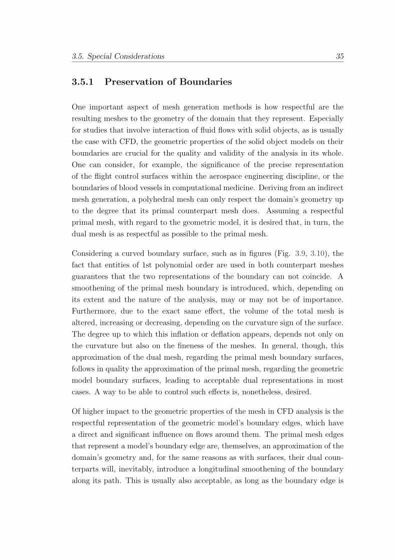
Considering a curved boundary surface, such as in figures (Fig. 3.9, 3.10), the
fact that entities of 1st polynomial order are used in both counterpart meshes
guarantees that the two representations of the boundary can not coincide. A
smoothening of the primal mesh boundary is introduced, which, depending on
its extent and the nature of the analysis, may or may not be of importance.
Furthermore, due to the exact same effect, the volume of the total mesh is
altered, increasing or decreasing, depending on the curvature sign of the surface.
The degree up to which this inflation or deflation appears, depends not only on
the curvature but also on the fineness of the meshes. In general, though, this
approximation of the dual mesh, regarding the primal mesh boundary surfaces,
follows in quality the approximation of the primal mesh, regarding the geometric
model boundary surfaces, leading to acceptable dual representations in most
cases. A way to be able to control such effects is, nonetheless, desired.
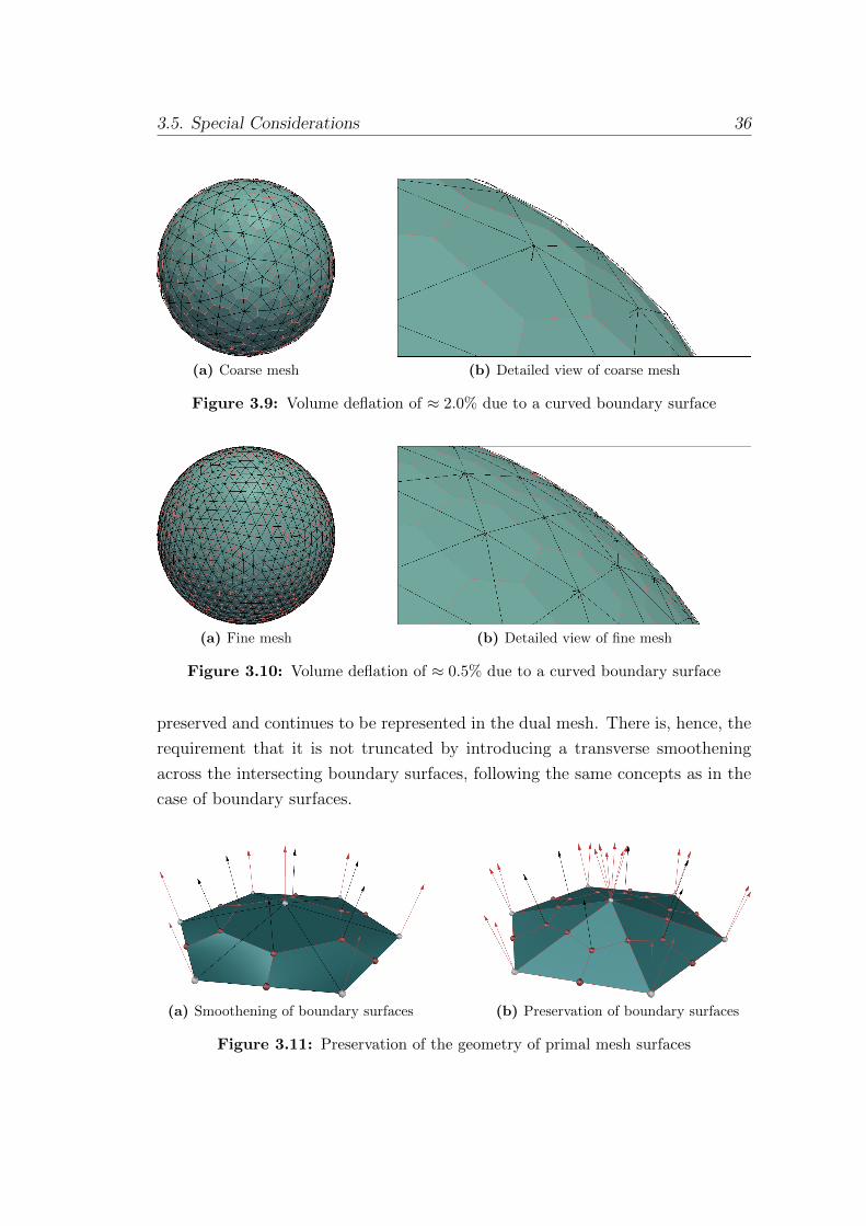
Of higher impact to the geometric properties of the mesh in CFD analysis is the
respectful representation of the geometric model’s boundary edges, which have
a direct and significant influence on flows around them. The primal mesh edges
that represent a model’s boundary edge are, themselves, an approximation of the
domain’s geometry and, for the same reasons as with surfaces, their dual coun-
terparts will, inevitably, introduce a longitudinal smoothening of the boundary
along its path. This is usually also acceptable, as long as the boundary edge is
3.5. Special Considerations 36
(a) Coarse mesh (b) Detailed view of coarse mesh
Figure 3.9: Volume deflation of ≈ 2.0% due to a curved boundary surface
(a) Fine mesh (b) Detailed view of fine mesh
Figure 3.10: Volume deflation of ≈ 0.5% due to a curved boundary surface
preserved and continues to be represented in the dual mesh. There is, hence, the
requirement that it is not truncated by introducing a transverse smoothening
across the intersecting boundary surfaces, following the same concepts as in the
case of boundary surfaces.
(a) Smoothening of boundary surfaces (b) Preservation of boundary surfaces
Figure 3.11: Preservation of the geometry of primal mesh surfaces
3.5. Special Considerations 37
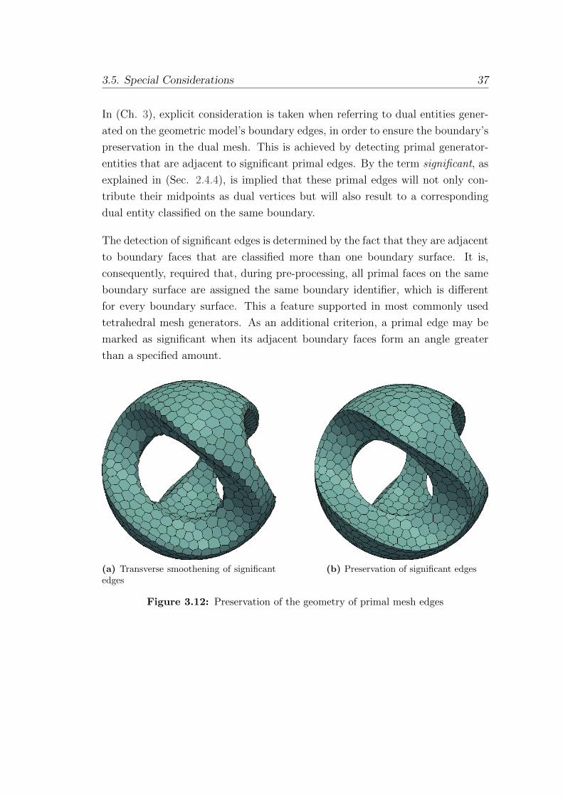
In (Ch. 3), explicit consideration is taken when referring to dual entities gener-
ated on the geometric model’s boundary edges, in order to ensure the boundary’s
preservation in the dual mesh. This is achieved by detecting primal generator-
entities that are adjacent to significant primal edges. By the term significant, as
explained in (Sec. 2.4.4), is implied that these primal edges will not only con-
tribute their midpoints as dual vertices but will also result to a corresponding
dual entity classified on the same boundary.
The detection of significant edges is determined by the fact that they are adjacent
to boundary faces that are classified more than one boundary surface. It is,
consequently, required that, during pre-processing, all primal faces on the same
boundary surface are assigned the same boundary identifier, which is different
for every boundary surface. This a feature supported in most commonly used
tetrahedral mesh generators. As an additional criterion, a primal edge may be
marked as significant when its adjacent boundary faces form an angle greater
than a specified amount.
(a) Transverse smoothening of significantedges
(b) Preservation of significant edges
Figure 3.12: Preservation of the geometry of primal mesh edges
3.5. Special Considerations 38
3.5.2 Internal Boundaries
Special care is required at areas where boundaries are present, within the 3D do-
main. In general, two different situations may result in the formation of internal
boundaries, which require separate treatment.
One case includes voids completely enclosed by the 3D volume. Even though
these voids form geometric boundaries that are in the interior of the domain,
from a topological perspective they can be treated exactly the same way external
boundaries are. Such areas, that denote a distinction between the continuum
material and the absence of it, can be detected by assigning a boundary condition
and orienting external faces in such a way, that their normals point away, with
respect to the volume. In case of internal voids, it is sufficient that these normals,
already at the primal mesh, point towards the void “center” and not the material
(Fig. 3.13a – 3.13c).
However, there are cases where an internal surface is not used in order to distin-
guish between continuum or void areas, but rather to differentiate between areas
with different materials. Furthermore, internal boundaries may also be used to
explicitly state that a region within the domain should be preserved as in the
primal mesh, as elements of special interest are classified on this boundary. As
an example, this approach may be desired in order to preserve a region where
two blocks of different primal element types, within a mixed mesh, meet. Cur-
rently, the present implementation is not designed to handle such cases, however
it has been shown that with slight modifications, regarding the polyhedral mesh
generation rules, it is possible to account for this consideration [10].
3.5.3 Boundary Layer
The poor numerical properties of tetrahedral meshes have dictated the generation
of a thin layer of prismatic, pentahedral elements at the boundary. With this
common practice, analysts have been able to partially overcome the inability of
tetrahedra to capture the details of a flow at regions close to the boundary [23].
The appropriate generation of a corresponding boundary layer for polyhedral
3.5. Special Considerations 39
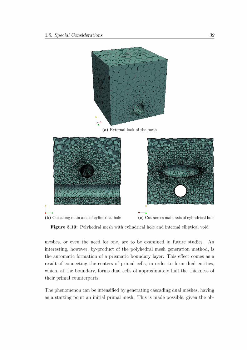
(a) External look of the mesh
(b) Cut along main axis of cylindrical hole (c) Cut across main axis of cylindrical hole
Figure 3.13: Polyhedral mesh with cylindrical hole and internal elliptical void
meshes, or even the need for one, are to be examined in future studies. An
interesting, however, by-product of the polyhedral mesh generation method, is
the automatic formation of a prismatic boundary layer. This effect comes as a
result of connecting the centers of primal cells, in order to form dual entities,
which, at the boundary, forms dual cells of approximately half the thickness of
their primal counterparts.
The phenomenon can be intensified by generating cascading dual meshes, having
as a starting point an initial primal mesh. This is made possible, given the ob-

3.5. Special Considerations 40
servation that the dual counterpart of a general bounded polyhedral mesh tends
to resemble the primal, tetrahedral mesh, with the exception at the boundaries.
This correspondence emerges in a similar way that the dual counterpart of a
Voronoi tessellation is a Delaunay triangulation / tetrahedralization, and vice
versa. Therefore, for each generation of meshes, the dual mesh that is obtained
serves as the primal mesh for the next iteration.
It can, then, be observed that for each generation, the boundary layer gets ap-
proximately half the thickness of that of the input mesh. Since two iterations
are needed in order to cascade from a polyhedral mesh to a tetrahedral domi-
nant and back to a polyhedral one, the formed boundary layer will conclude to
a thickness of a 14
factor. It is, however, apparent that with such an approach it
is difficult to control the properties and thickness of the formed boundary layer
and the application of this method seems of limited use.
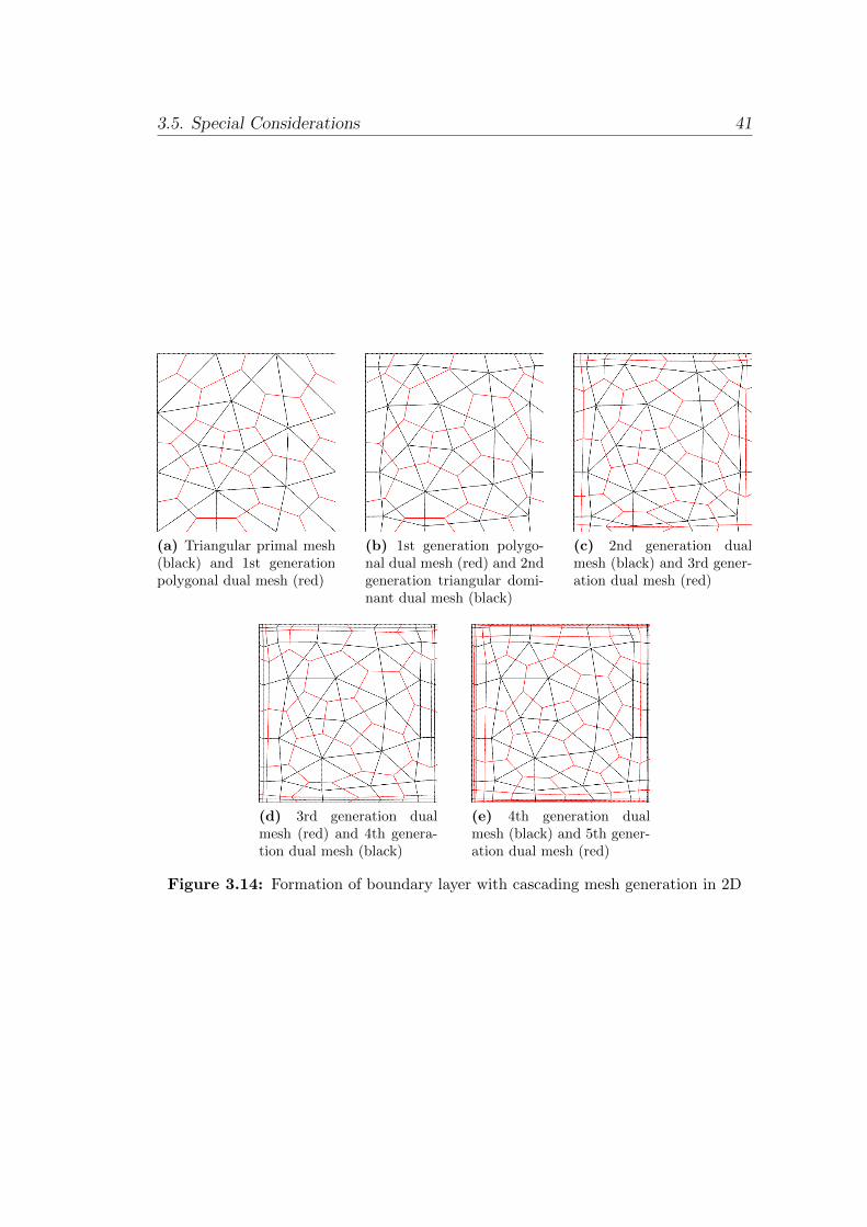
3.5. Special Considerations 41
(a) Triangular primal mesh(black) and 1st generationpolygonal dual mesh (red)
(b) 1st generation polygo-nal dual mesh (red) and 2ndgeneration triangular domi-nant dual mesh (black)
(c) 2nd generation dualmesh (black) and 3rd gener-ation dual mesh (red)
(d) 3rd generation dualmesh (red) and 4th genera-tion dual mesh (black)
(e) 4th generation dualmesh (black) and 5th gener-ation dual mesh (red)
Figure 3.14: Formation of boundary layer with cascading mesh generation in 2D
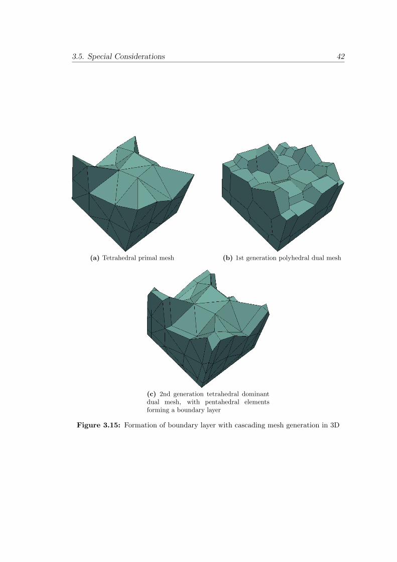
3.5. Special Considerations 42
(a) Tetrahedral primal mesh (b) 1st generation polyhedral dual mesh
(c) 2nd generation tetrahedral dominantdual mesh, with pentahedral elementsforming a boundary layer
Figure 3.15: Formation of boundary layer with cascading mesh generation in 3D
43
Chapter 4
Polyhedral Mesh Optimization
4.1 Introduction
Following the procedure described in the previous chapter, it is possible to obtain
a conforming dual mesh that respects the boundaries of the geometric model, the
properties of which are directly and solely dependent on those of the primal mesh.
However, it is desired that an analyst should have more control over the mesh
generation procedure, in order to obtain meshes of high quality. That being said,
one aspect to take into consideration is that mesh validity and quality cannot
always be clearly defined but are, rather, concepts that largely depend on the
context of use. This is something that applies even for tetrahedral and hexahedral
meshes, where validity and quality criteria may vary upon the simulation type
and the analysis software. Nevertheless, polyhedra are, in general, considered
of not as strict quality criteria, making polyhedral meshes a much more flexible
alternative for CFD simulations. In this chapter, an insight to the characteristics
that define the quality of a polyhedral mesh is attempted, as well as a description
of pre- and post-processing steps that may be applied, in order to optimize the
resulting mesh.

4.2. Validity 44
4.2 Validity
Depending on the simulation software, polyhedral elements that will satisfy the
validity criteria may range from those that provide a non-negative Jacobian at
quadrature points, to those that have a strictly positive insphere to circumsphere
ratio, with the latter being, for non-simplices, loosely defined. A conservative
approach that is likely to satisfy most analysis codes was suggested by Garimella
et al., according to which, a polyhedron is considered valid if it passes the star-
shaped test [10].
In this method, a measure of convexity is provided, which considers a symmetric
decomposition of each polyhedron into tetrahedra. The tetrahedralization takes
place around a universal apex at a “central point” of the volume, connected with
a base triangle formed by a “central point” of each face and the vertices of the
faces, considered in pairs 4.1. In the above procedure, the geometric mean of
the vertices of a face may be regarded its center and the same applies for the
polyhedral volume. The polyhedron is valid when the signed volume of each of
the formed tetrahedra is positive.
In the present work, validity of dual meshes has been specifically resolved ac-
cording to behavior of the computational tools in hand. The primal tetrahedral
meshes, generated by NETGEN mesh generator [18], have, in general, resulted
into convex dual polyhedra in the interior, with the occasional presence of slightly
non-planar faces. Although this is a factor that may influence convergence and
accuracy properties, it has not been an issue, regarding cell validity, for DOL-
FYN CFD code [3], which has been used as provided within the environment of
SOFiSTiK FEA software [1].
However, invalid polyhedra have appeared at reentrant corners of geometric mod-
els with sharp concavities. In theses cases, highly concave cells were formed, the
centroids of which was located outside the volume of the element, causing the
CFD analysis to fail. In order to overcome this restraining effect, an initial so-
lution has been to manually shift the centroids of such elements to a location
within their volume. Although this remedy cannot be considered optimal, Dol-
fyn’s validity criteria have been, this way, satisfied and simulations including
domains with sharp concavities have been successfully run. Further discussion

4.3. Quality 45
Figure 4.1: Decomposition of polyhedral cell during the star-shaped test
on the effects of this approach on convergence and accuracy is made in (Ch. 5).
4.3 Quality
4.3.1 Selection of Central Points
In the previous chapters, generation of dual meshes has been described using the
generic term of central point, when referring to a point lying, in general, withing
the boundaries of a face or a volume, while, for edges, the unambiguous term
midpoint is used. These central points define positions of generated dual vertices
and their computation is probably the most decisive part of the procedure, having
a major impact on the validity and quality of the resulting polyhedra.
A common choice for central points of faces and volumes are their centroids,
which are easily computed even for arbitrarily-shaped entities, by performing a
decomposition to triangles or tetrahedra, respectively. The advantage of using
centroids is that they are always positioned withing their parent-entity, avoiding
this way overlapping entities. However, dual faces formed of dual vertices on
primal entities’ centroids are usually non-planar, introducing local concavities
and computationally poor properties to the polyhedra (Fig. 4.2).
For tetrahedral meshes, however, which are the primal meshes of preference in
most cases, an alternative “central point” is the triangular faces’ and the tetrahe-
dra’s circumcenter, as these simplices are always circumscribable. The advantage
of using circumcenters is that the resulting dual faces are always planar and, in
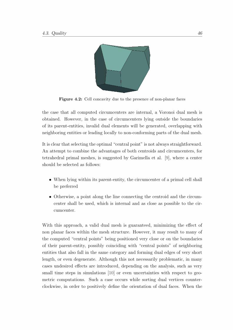
4.3. Quality 46
Figure 4.2: Cell concavity due to the presence of non-planar faces
the case that all computed circumcenters are internal, a Voronoi dual mesh is
obtained. However, in the case of circumcenters lying outside the boundaries
of its parent-entities, invalid dual elements will be generated, overlapping with
neighboring entities or leading locally to non-conforming parts of the dual mesh.
It is clear that selecting the optimal “central point” is not always straightforward.
An attempt to combine the advantages of both centroids and circumcenters, for
tetrahedral primal meshes, is suggested by Garimella et al. [9], where a center
should be selected as follows:
• When lying within its parent-entity, the circumcenter of a primal cell shall
be preferred
• Otherwise, a point along the line connecting the centroid and the circum-
center shall be used, which is internal and as close as possible to the cir-
cumcenter.
With this approach, a valid dual mesh is guaranteed, minimizing the effect of
non planar faces within the mesh structure. However, it may result to many of
the computed “central points” being positioned very close or on the boundaries
of their parent-entity, possibly coinciding with “central points” of neighboring
entities that also fall in the same category and forming dual edges of very short
length, or even degenerate. Although this not necessarily problematic, in many
cases undesired effects are introduced, depending on the analysis, such as very
small time steps in simulations [10] or even uncertainties with respect to geo-
metric computations. Such a case occurs while sorting dual vertices counter-
clockwise, in order to positively define the orientation of dual faces. When the
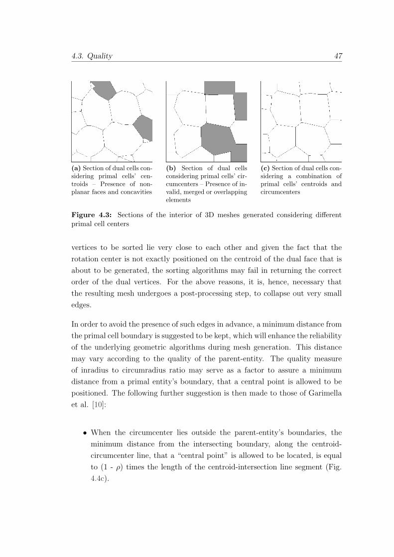
4.3. Quality 47
(a) Section of dual cells con-sidering primal cells’ cen-troids – Presence of non-planar faces and concavities
(b) Section of dual cellsconsidering primal cells’ cir-cumcenters – Presence of in-valid, merged or overlappingelements
(c) Section of dual cells con-sidering a combination ofprimal cells’ centroids andcircumcenters
Figure 4.3: Sections of the interior of 3D meshes generated considering differentprimal cell centers
vertices to be sorted lie very close to each other and given the fact that the
rotation center is not exactly positioned on the centroid of the dual face that is
about to be generated, the sorting algorithms may fail in returning the correct
order of the dual vertices. For the above reasons, it is, hence, necessary that
the resulting mesh undergoes a post-processing step, to collapse out very small
edges.
In order to avoid the presence of such edges in advance, a minimum distance from
the primal cell boundary is suggested to be kept, which will enhance the reliability
of the underlying geometric algorithms during mesh generation. This distance
may vary according to the quality of the parent-entity. The quality measure
of inradius to circumradius ratio may serve as a factor to assure a minimum
distance from a primal entity’s boundary, that a central point is allowed to be
positioned. The following further suggestion is then made to those of Garimella
et al. [10]:
• When the circumcenter lies outside the parent-entity’s boundaries, the
minimum distance from the intersecting boundary, along the centroid-
circumcenter line, that a “central point” is allowed to be located, is equal
to (1 - ρ) times the length of the centroid-intersection line segment (Fig.
4.4c).

4.3. Quality 48
Considering a vector with its origin at the centroid, the above can be
expressed as (Eq. 4.1):
−−→CdC =
−−−→CdCr
‖−−−→CdCr ‖
·min
‖−−−→CdCr ‖
ρs ‖−−→CdI ‖ , ρs ∈ [0, 1]
(4.1)
where ρs is a reduction factor which depends on the cell quality , Cd the
centroid, Cr the circumcenter, I the aforementioned intersection and C is
the internal point where the dual vertex will be located. The common
simplices’ shape measure that considers the inradius - circumradius ratio
[14] has been found to serve well for this purpose (Eq. 4.2).
ρtr =2Rin
Rcirc
, ρtet =3Rin
Rcirc
(4.2)
(a) Dual vertex located on the circumcen-ter of a well-centered primal cell
(b) Dual vertex located at an internalpoint, when the circumcenter is internalbut very close to the primal cell boundary
(c) Dual vertex located at an internalpoint of a flat primal cell
Figure 4.4: Location of dual vertices for various cases of primal cell quality

4.3. Quality 49
The impact of this additional criterion for selecting “central points” has a minor
impact on the shape of the resulting polyhedra, improving the polyhedra’s angles
at this regions but increasing slightly the non-planar effect of those dual faces
whose vertices have been affected. The algorithmic stability, however, of the
overall dual mesh generation is significantly improved.
4.3.2 Untangling and Smoothing
Given the difficulty to establish unique criteria to measure the quality of polyhe-
dra, several suggestions are encountered in literature, regarding the optimization
of polyhedral meshes. A notable effort has been done by Vartziotis and Him-
pel, wherein the gradient flow of the mean volume of the tetrahedra, formed by
decomposing polyhedral elements, is considered [33, 34].
In a more algorithmic-centric approach, improvements for a polygonal surface
mesh have been discussed in the past [9], while Dyadechko et al. provide a
method for minimizing a global objective function, which considers the sum of
a condition number introduced for the corners of polyhedral elements [5]. In
this effort, the mesh vertices are repositioned in a minimalistic way, eliminating
ill-shaped elements, while keeping the mesh as close as possible to the original
one. In the near future, research on a multi-objective optimization is expected,
in an attempt to improve the planarity of polyhedral faces [10].

50
Chapter 5
Validation and Conclusions
5.1 Introduction
The polyhedral mesh generator that has been implemented, has served, apart
from the proof of concept, as a tool for exploring the dominant characteristics
of polyhedral meshes within the field of CFD simulation. One thing to consider
is the fact that mesh generation, itself, is a pre-processing task that may claim
a major proportion of the required analysis time. Another significant aspect is
the influence of the mesh on the numerics of the analysis, regarding convergence
and accuracy. In the following sections, the use of polyhedral meshes in CFD is
evaluated, having in mind the impact of meshing on the overall analysis perfor-
mance. In order to do so, a number of different study cases have been considered,
for each of which a polyhedral mesh has been generated and exported. This has
served as a geometry input file for DOLFYN CFD code [3], as is provided within
the environment of SOFiSTiK FEA software [1].
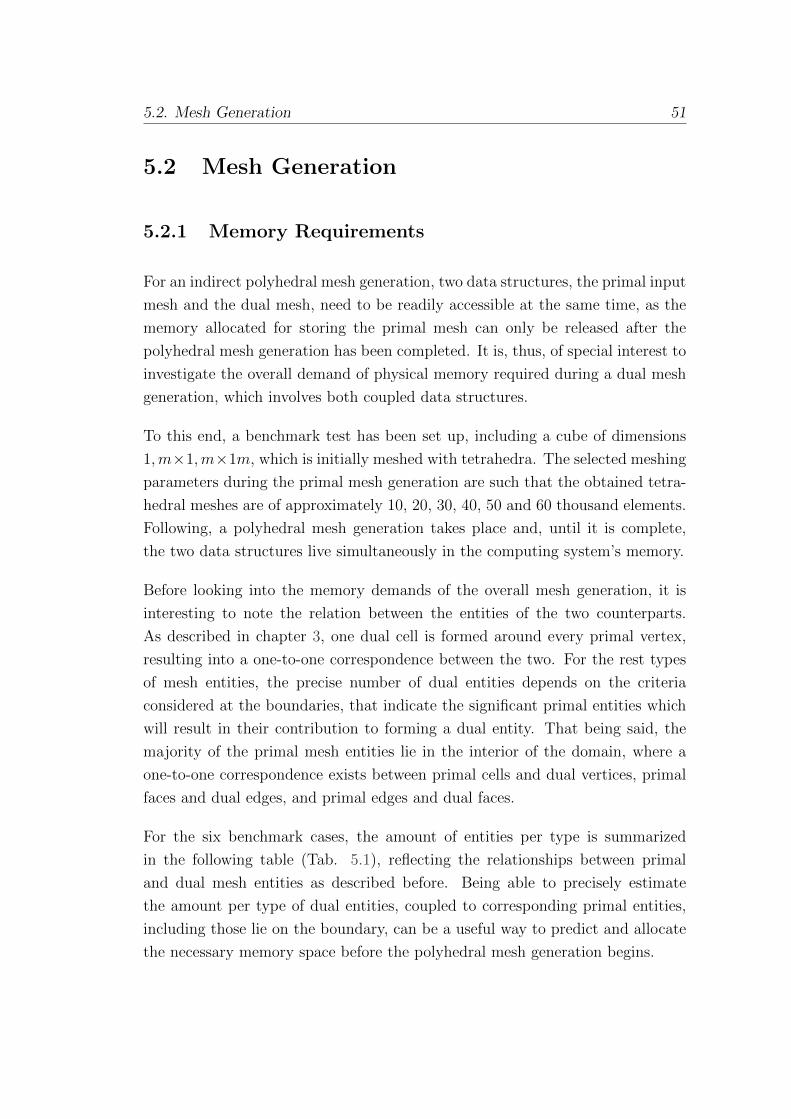
5.2. Mesh Generation 51
5.2 Mesh Generation
5.2.1 Memory Requirements
For an indirect polyhedral mesh generation, two data structures, the primal input
mesh and the dual mesh, need to be readily accessible at the same time, as the
memory allocated for storing the primal mesh can only be released after the
polyhedral mesh generation has been completed. It is, thus, of special interest to
investigate the overall demand of physical memory required during a dual mesh
generation, which involves both coupled data structures.
To this end, a benchmark test has been set up, including a cube of dimensions
1,m×1,m×1m, which is initially meshed with tetrahedra. The selected meshing
parameters during the primal mesh generation are such that the obtained tetra-
hedral meshes are of approximately 10, 20, 30, 40, 50 and 60 thousand elements.
Following, a polyhedral mesh generation takes place and, until it is complete,
the two data structures live simultaneously in the computing system’s memory.
Before looking into the memory demands of the overall mesh generation, it is
interesting to note the relation between the entities of the two counterparts.
As described in chapter 3, one dual cell is formed around every primal vertex,
resulting into a one-to-one correspondence between the two. For the rest types
of mesh entities, the precise number of dual entities depends on the criteria
considered at the boundaries, that indicate the significant primal entities which
will result in their contribution to forming a dual entity. That being said, the
majority of the primal mesh entities lie in the interior of the domain, where a
one-to-one correspondence exists between primal cells and dual vertices, primal
faces and dual edges, and primal edges and dual faces.
For the six benchmark cases, the amount of entities per type is summarized
in the following table (Tab. 5.1), reflecting the relationships between primal
and dual mesh entities as described before. Being able to precisely estimate
the amount per type of dual entities, coupled to corresponding primal entities,
including those lie on the boundary, can be a useful way to predict and allocate
the necessary memory space before the polyhedral mesh generation begins.
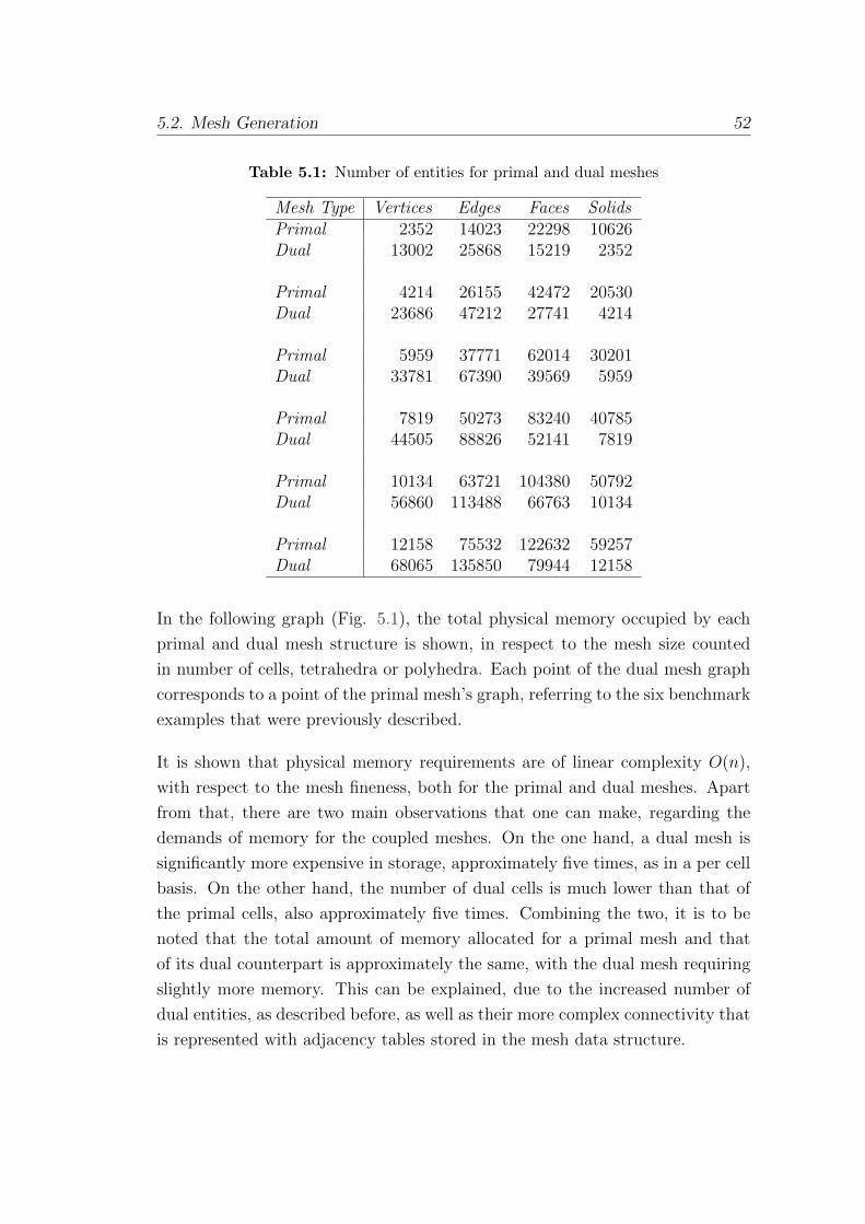
5.2. Mesh Generation 52
Table 5.1: Number of entities for primal and dual meshes
Mesh Type Vertices Edges Faces SolidsPrimal 2352 14023 22298 10626Dual 13002 25868 15219 2352
Primal 4214 26155 42472 20530Dual 23686 47212 27741 4214
Primal 5959 37771 62014 30201Dual 33781 67390 39569 5959
Primal 7819 50273 83240 40785Dual 44505 88826 52141 7819
Primal 10134 63721 104380 50792Dual 56860 113488 66763 10134
Primal 12158 75532 122632 59257Dual 68065 135850 79944 12158
In the following graph (Fig. 5.1), the total physical memory occupied by each
primal and dual mesh structure is shown, in respect to the mesh size counted
in number of cells, tetrahedra or polyhedra. Each point of the dual mesh graph
corresponds to a point of the primal mesh’s graph, referring to the six benchmark
examples that were previously described.
It is shown that physical memory requirements are of linear complexity O(n),
with respect to the mesh fineness, both for the primal and dual meshes. Apart
from that, there are two main observations that one can make, regarding the
demands of memory for the coupled meshes. On the one hand, a dual mesh is
significantly more expensive in storage, approximately five times, as in a per cell
basis. On the other hand, the number of dual cells is much lower than that of
the primal cells, also approximately five times. Combining the two, it is to be
noted that the total amount of memory allocated for a primal mesh and that
of its dual counterpart is approximately the same, with the dual mesh requiring
slightly more memory. This can be explained, due to the increased number of
dual entities, as described before, as well as their more complex connectivity that
is represented with adjacency tables stored in the mesh data structure.

5.2. Mesh Generation 53
Figure 5.1: Memory requirements for tetrahedral meshes and their polyhedral coun-terparts
What can be, finally, drawn as a conclusion, regarding storage space requirements
in polyhedral mesh generation, is that for a given geometry one should account
for a further memory needs, during the mesh generation itself, that is in general
within acceptable bounds given the modern computing systems capabilities. In
the benchmark examples above, approximately the same amount of physical
memory, as that of the tetrahedral input mesh, is additionally allocated for
the dual mesh. However, after the polyhedral mesh generation is complete, the
memory occupied by the primal mesh may be released and the system’s resources
are free to be used otherwise.
5.2.2 Performance
Figure (Fig. 5.2) shows how mesh generation time is related to the mesh size, for
primal as well as dual meshes. The graphs refer to the same geometry of a unit
cube, which was meshed primarily with tetrahedra, using increasing fineness,
and their counterpart polyhedral dual meshes. Therefore, the marked points on
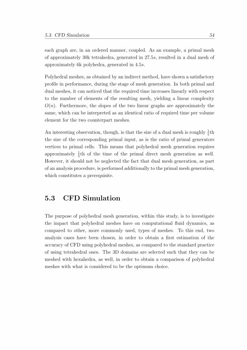
5.3. CFD Simulation 54
each graph are, in an ordered manner, coupled. As an example, a primal mesh
of approximately 30k tetrahedra, generated in 27.5s, resulted in a dual mesh of
approximately 6k polyhedra, generated in 4.5s.
Polyhedral meshes, as obtained by an indirect method, have shown a satisfactory
profile in performance, during the stage of mesh generation. In both primal and
dual meshes, it can noticed that the required time increases linearly with respect
to the number of elements of the resulting mesh, yielding a linear complexity
O(n). Furthermore, the slopes of the two linear graphs are approximately the
same, which can be interpreted as an identical ratio of required time per volume
element for the two counterpart meshes.
An interesting observation, though, is that the size of a dual mesh is roughly 15th
the size of the corresponding primal input, as is the ratio of primal generators
vertices to primal cells. This means that polyhedral mesh generation requires
approximately 15th of the time of the primal direct mesh generation as well.
However, it should not be neglected the fact that dual mesh generation, as part
of an analysis procedure, is performed additionally to the primal mesh generation,
which constitutes a prerequisite.
5.3 CFD Simulation
The purpose of polyhedral mesh generation, within this study, is to investigate
the impact that polyhedral meshes have on computational fluid dynamics, as
compared to other, more commonly used, types of meshes. To this end, two
analysis cases have been chosen, in order to obtain a first estimation of the
accuracy of CFD using polyhedral meshes, as compared to the standard practice
of using tetrahedral ones. The 3D domains are selected such that they can be
meshed with hexahedra, as well, in order to obtain a comparison of polyhedral
meshes with what is considered to be the optimum choice.
5.3. CFD Simulation 55
Figure 5.2: Polyhedral mesh generation time in comparison with corresponding pri-mal mesh generation
5.3.1 Laminar Flow Through Cube
In this case study, air flows through a unit volume (Fig. 5.3) with a laminar flow
of velocity:
Ux = 1.0m/s, Uy = 0.0m/s, Uz = 0.0m/s
The volume is meshed with two directly comparable ways: with a hexahedral
mesh and with a polyhedral mesh of approximately the same number of cells.
Additionally, the tetrahedral primal mesh that was used in order to generate
the polyhedral one, is considered as well (Fig. 5.4a – 5.4b). This allows for a
comparison between primal and dual meshes, rather than uncoupled tetrahedral
and polyhedral meshes or tetrahedral and hexahedral ones. During the analysis,
the residuum of Ux is monitored with respect to the number of iteration steps.
What is made clear in graph (Fig. 5.5) is that using the tetrahedral primal
mesh, the analysis is unable to converge to the level of the desired tolerance. On

5.3. CFD Simulation 56
Figure 5.3: Unit cube with laminar flow along a main axis
the other hand, the hexahedral mesh shows a satisfactory analysis progression,
approaching to convergence after approximately 60 iterations and stabilizing at
approximately 80 iterations. Finally, the polyhedral dual mesh reaches a conver-
gence status at approximately 80 iterations as well.
An interesting remark is that when using polyhedra, while progression towards
convergence is noticeably slower than when using hexahedra, a much more sta-
ble analysis profile is achieved, with fewer numerical oscillations, mainly concen-
trated at the beginning of the analysis. This can be explained by the fact that,
despite the structured hexahedral mesh lacking any geometrically poor quality
elements, the connectivity of polyhedral elements with their neighboring cells
is significantly higher, allowing for fluxes of any direction to be accounted for
during the finite volume analysis. On the other hand, out of the 26 neighboring
cells enclosing an internal hexahedron, 6 of them share a common face with it,
allowing only fluxes along the three main directions to be considered.
Finally, considering the convergence progression of the tetrahedral mesh, as well,
table (Tab. 5.2) shows the number of iterations that are required in order for
the three types of meshes to conclude to the same level of convergence, dictated
by the minimum residuum an analysis with tetrahedra can conclude to.

5.3. CFD Simulation 57
(a) Primal tetrahedral mesh (b) Dual polyhedral mesh
(c) Reference hexahedral mesh
Figure 5.4: Tetrahedral, polyhedral and hexahedral meshing of the 3D domain
Table 5.2: Iterations needed to achieve the same level of convergence
Mesh Type Number of Cells IterationsTetrahedral 6168 229Polyhedral 1336 28Hexahedral 1331 24
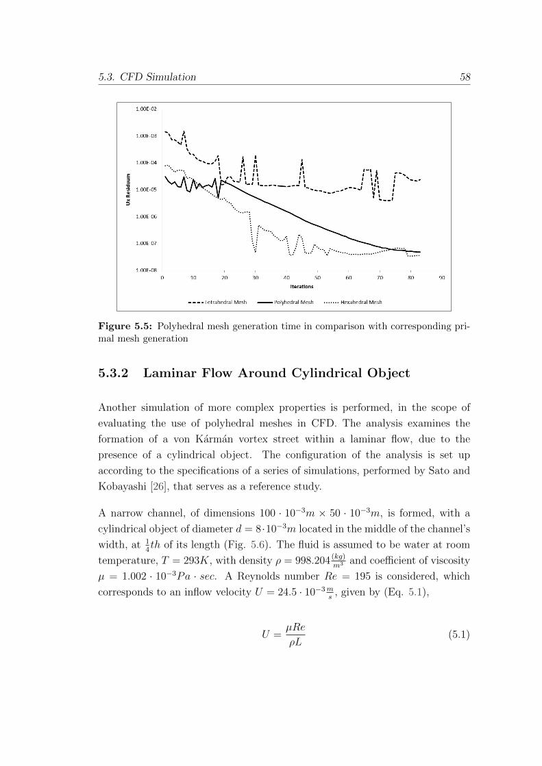
5.3. CFD Simulation 58
Figure 5.5: Polyhedral mesh generation time in comparison with corresponding pri-mal mesh generation
5.3.2 Laminar Flow Around Cylindrical Object
Another simulation of more complex properties is performed, in the scope of
evaluating the use of polyhedral meshes in CFD. The analysis examines the
formation of a von Karman vortex street within a laminar flow, due to the
presence of a cylindrical object. The configuration of the analysis is set up
according to the specifications of a series of simulations, performed by Sato and
Kobayashi [26], that serves as a reference study.
A narrow channel, of dimensions 100 · 10−3m × 50 · 10−3m, is formed, with a
cylindrical object of diameter d = 8·10−3m located in the middle of the channel’s
width, at 14th of its length (Fig. 5.6). The fluid is assumed to be water at room
temperature, T = 293K, with density ρ = 998.204 (kg)m3 and coefficient of viscosity
µ = 1.002 · 10−3Pa · sec. A Reynolds number Re = 195 is considered, which
corresponds to an inflow velocity U = 24.5 · 10−3ms
, given by (Eq. 5.1),
U =µRe
ρL(5.1)
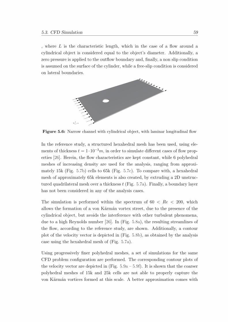
5.3. CFD Simulation 59
, where L is the characteristic length, which in the case of a flow around a
cylindrical object is considered equal to the object’s diameter. Additionally, a
zero pressure is applied to the outflow boundary and, finally, a non slip condition
is assumed on the surface of the cylinder, while a free-slip condition is considered
on lateral boundaries.
Figure 5.6: Narrow channel with cylindrical object, with laminar longitudinal flow
In the reference study, a structured hexahedral mesh has been used, using ele-
ments of thickness t = 1 ·10−3m, in order to simulate different cases of flow prop-
erties [26]. Herein, the flow characteristics are kept constant, while 6 polyhedral
meshes of increasing density are used for the analysis, ranging from approxi-
mately 15k (Fig. 5.7b) cells to 65k (Fig. 5.7c). To compare with, a hexahedral
mesh of approximately 65k elements is also created, by extruding a 2D unstruc-
tured quadrilateral mesh over a thickness t (Fig. 5.7a). Finally, a boundary layer
has not been considered in any of the analysis cases.
The simulation is performed within the spectrum of 60 < Re < 200, which
allows the formation of a von Karman vortex street, due to the presence of the
cylindrical object, but avoids the interference with other turbulent phenomena,
due to a high Reynolds number [26]. In (Fig. 5.8a), the resulting streamlines of
the flow, according to the reference study, are shown. Additionally, a contour
plot of the velocity vector is depicted in (Fig. 5.8b), as obtained by the analysis
case using the hexahedral mesh of (Fig. 5.7a).
Using progressively finer polyhedral meshes, a set of simulations for the same
CFD problem configuration are performed. The corresponding contour plots of
the velocity vector are depicted in (Fig. 5.9a – 5.9f). It is shown that the coarser
polyhedral meshes of 15k and 25k cells are not able to properly capture the
von Karman vortices formed at this scale. A better approximation comes with
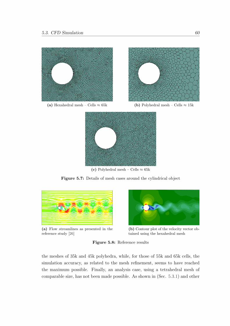
5.3. CFD Simulation 60
(a) Hexahedral mesh – Cells ≈ 65k (b) Polyhedral mesh – Cells ≈ 15k
(c) Polyhedral mesh – Cells ≈ 65k
Figure 5.7: Details of mesh cases around the cylindrical object
(a) Flow streamlines as presented in thereference study [26]
(b) Contour plot of the velocity vector ob-tained using the hexahedral mesh
Figure 5.8: Reference results
the meshes of 35k and 45k polyhedra, while, for those of 55k and 65k cells, the
simulation accuracy, as related to the mesh refinement, seems to have reached
the maximum possible. Finally, an analysis case, using a tetrahedral mesh of
comparable size, has not been made possible. As shown in (Sec. 5.3.1) and other

5.3. CFD Simulation 61
studies [21, 28], this would have required a mesh refinement of more than 5 times
tetrahedral elements than the number of polyhedra.
(a) Polyhedral mesh – Cells ≈ 15k (b) Polyhedral mesh – Cells ≈ 25k
(c) Polyhedral mesh – Cells ≈ 35k (d) Polyhedral mesh – Cells ≈ 45k
(e) Polyhedral mesh – Cells ≈ 55k (f) Polyhedral mesh – Cells ≈ 65k
Figure 5.9: Contour plots of the velocity vector for increasing mesh refinement ofpolyhedral meshes
It should be noted that the contour plots become growingly speckled, as the mesh
refinement increases. This can be explained by the fact that an extrapolation of
the result positions is made, during post-processing. The computed values, at the
centers of the polyhedral cells, are transfered to the vertices of the primal mesh,
in order to visualize the results. This causes inconsistencies in the contour plot,
that may be overcome by importing the actual result locations in the visualization
software, or by applying a bilinear, or other, interpolation of the obtained results,
for the positions of the primal vertices.
During the CFD simulation, the component Ux of the flow velocity is monitored
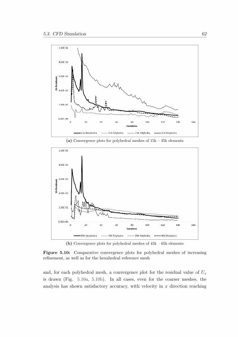
5.3. CFD Simulation 62
(a) Convergence plots for polyhedral meshes of 15k – 35k elements
(b) Convergence plots for polyhedral meshes of 45k – 65k elements
Figure 5.10: Comparative convergence plots for polyhedral meshes of increasingrefinement, as well as for the hexahedral reference mesh
and, for each polyhedral mesh, a convergence plot for the residual value of Ux
is drawn (Fig. 5.10a, 5.10b). In all cases, even for the coarser meshes, the
analysis has shown satisfactory accuracy, with velocity in x direction reaching
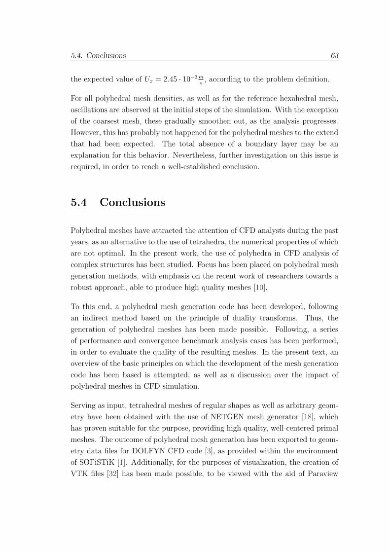
5.4. Conclusions 63
the expected value of Ux = 2.45 · 10−3ms
, according to the problem definition.
For all polyhedral mesh densities, as well as for the reference hexahedral mesh,
oscillations are observed at the initial steps of the simulation. With the exception
of the coarsest mesh, these gradually smoothen out, as the analysis progresses.
However, this has probably not happened for the polyhedral meshes to the extend
that had been expected. The total absence of a boundary layer may be an
explanation for this behavior. Nevertheless, further investigation on this issue is
required, in order to reach a well-established conclusion.
5.4 Conclusions
Polyhedral meshes have attracted the attention of CFD analysts during the past
years, as an alternative to the use of tetrahedra, the numerical properties of which
are not optimal. In the present work, the use of polyhedra in CFD analysis of
complex structures has been studied. Focus has been placed on polyhedral mesh
generation methods, with emphasis on the recent work of researchers towards a
robust approach, able to produce high quality meshes [10].
To this end, a polyhedral mesh generation code has been developed, following
an indirect method based on the principle of duality transforms. Thus, the
generation of polyhedral meshes has been made possible. Following, a series
of performance and convergence benchmark analysis cases has been performed,
in order to evaluate the quality of the resulting meshes. In the present text, an
overview of the basic principles on which the development of the mesh generation
code has been based is attempted, as well as a discussion over the impact of
polyhedral meshes in CFD simulation.
Serving as input, tetrahedral meshes of regular shapes as well as arbitrary geom-
etry have been obtained with the use of NETGEN mesh generator [18], which
has proven suitable for the purpose, providing high quality, well-centered primal
meshes. The outcome of polyhedral mesh generation has been exported to geom-
etry data files for DOLFYN CFD code [3], as provided within the environment
of SOFiSTiK [1]. Additionally, for the purposes of visualization, the creation of
VTK files [32] has been made possible, to be viewed with the aid of Paraview
5.4. Conclusions 64
visualization software [35].
The overall complexity of the mesh generation algorithm has proved to be linear,
requiring the same amount of computational effort per cell, as needed by the
tetrahedral mesh generator that has been used. However, due to the fact that
the total number of elements of a polyhedral mesh is about 5 times less than
those of its primal, approximately frac15th of the corresponding time is needed.
It should be emphasized, though, that the computational effort, which is required
for polyhedral mesh generation, should be regarded as additional to that of
generating a primal mesh.
In terms of storage, a linear complexity has been observed as well, even though
the sophisticated topology of polyhedral meshes requires the use of data struc-
tures that occupy significantly larger amount of memory per cell, as compared
to a tetrahedral mesh. The fact, however, that the number of elements of a
polyhedral mesh is far lower than its primal, leads to the two meshes requiring
approximately the same amount of storage. This means that, at its peak, the
required space in memory becomes two times larger than storing only a tetra-
hedral mesh. In this area there is certainly room for future improvements, by
carefully selecting the mesh representation schemes that are being used, as well
as optimizing their implementation.
Regarding the influence of polyhedral meshes on CFD simulation, despite the in-
crease in absolute time required during mesh generation, the performance speed-
up during analysis has been observed to more than compensate for the increased
pre-processing effort. Polyhedral meshes, that provide the same level of accuracy
as tetrahedral ones, are of significantly less elements, which eventually leads to
faster and more accurate simulations. Finally, the above observations, regarding
performance and accuracy, seem to conform with the conclusions that have been
drawn by other studies in the past [21, 23].
With the current implementation, a conforming polyhedral mesh is obtained,
respecting the boundaries of the domain as described by the primal mesh. In
future efforts, post-processing steps may be applied to the mesh, in order to
optimize its topological and geometric properties. Garimella et al. [10] have
adequately described a first optimization approach for the geometric properties
of polyhedral cell. Focus is currently placed on multi-objective optimization, in

5.4. Conclusions 65
order to reduce the effect of non-planar dual faces. Furthermore, an attempt to
address the problem of concave cells at sharp reentrant corners is expected in
the near future. These are concepts that would be welcome in a future extension
of the present work.
To conclude with, polyhedral elements appear to combine the advantages of hex-
ahedra, in terms of performance and numerical properties, with those of tetrahe-
dra, in terms of flexibility for meshing domains of arbitrary geometry. Additional
testing and more detailed benchmark cases are needed, in order to further eval-
uate the properties of polyhedral meshes, and their influence on CFD analysis,
including cases of turbulent flows. The first indications obtained by the present
study show a promising future for polyhedra and, given the ongoing research,
there may be a time, not far in the future, when polyhedral meshing will be
regarded as standard practice within the scope of CFD analysis.
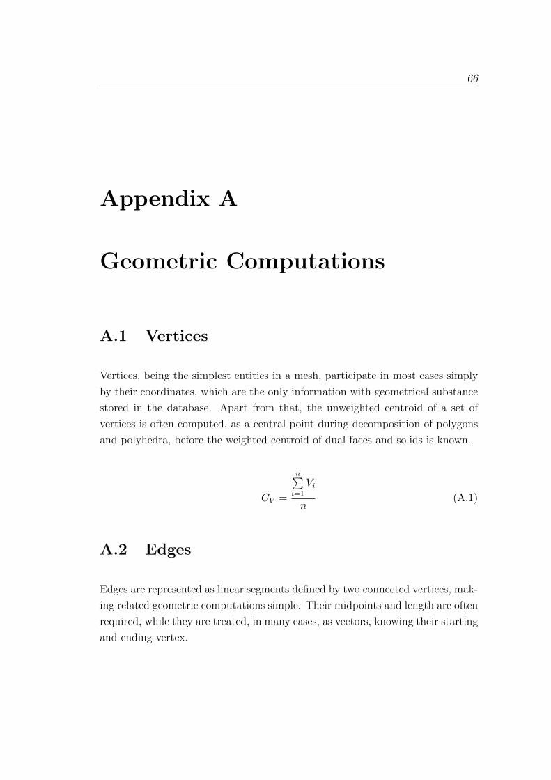
66
Appendix A
Geometric Computations
A.1 Vertices
Vertices, being the simplest entities in a mesh, participate in most cases simply
by their coordinates, which are the only information with geometrical substance
stored in the database. Apart from that, the unweighted centroid of a set of
vertices is often computed, as a central point during decomposition of polygons
and polyhedra, before the weighted centroid of dual faces and solids is known.
CV =
n∑i=1
Vi
n(A.1)
A.2 Edges
Edges are represented as linear segments defined by two connected vertices, mak-
ing related geometric computations simple. Their midpoints and length are often
required, while they are treated, in many cases, as vectors, knowing their starting
and ending vertex.

A.3. Faces 67
A.3 Faces
Dual faces are simple, non self-intersecting polygons, defined by an arbitrary
number of connected edges. Their shape can be irregular, which demands that
concave polygons, while not desirable, are not excluded from geometric algo-
rithms. Furthermore, it cannot be guaranteed that a face, formed by connecting
the centers of tetrahedra surrounding a primal edge, is always planar. To be able
to handle such arbitrary polygons, their decomposition to simplices is required,
commonly known as triangulation.
Figure A.1: Face decomposition by triangulation
The normal of polygons is computed by Newell’s formula, which is an efficient
way to compute face’s normals in 3D space [30]. Even in case of non-planar
faces, the algorithm is able to produce a vector, representing a uniform normal
perpendicular to a “mean” plane, for the set of points that form the polygon. In
general, this approach is sufficient, as faces are usually not highly non-planar, and
further sophisticated, computationally expensive solutions, such as least square
surface fitting, are not necessary.
NFx =n∑i=1
(yi − yi⊕1)(zi + zi⊕1) (A.2a)
NFy =n∑i=1
(zi − zi⊕1)(xi + xi⊕1) (A.2b)
NFz =n∑i=1
(xi − xi⊕1)(yi + yi⊕1) (A.2c)

A.4. Solids 68
Computing a polygon’s area, involves its decomposition into triangles and the
summation of the signed area of each triangle, in order to account for concave
shapes. The triangulation takes place using the face’s vertices’ centroid as a
decomposition center, as the polygon’s weighted centroid is not yet known. Fi-
nally, as the face may not be planar, the computed area is projected to the plane
dictated by the previously computed normal. Considering all the above, the area
is computed as shown by (Eq. A.3):
AF = N ·
n∑i=1
−−−→CV Vi ×
−−−−→CV Vi⊕1
2(A.3)
Following the same concept, a polygon’s centroid is computed by decomposing
the face.
CF =
n∑i=1
AiCi
AF(A.4)
where Ai stands for the signed area and Ci for the centroid of each triangle,
formed by two sequential vertices of the faces and the centroid of all of its vertices.
A.4 Solids
Extending the approach followed for geometric computations of polygons, polyhe-
dra are treated by applying a decomposition as well. This type of decomposition
is known as tetrahedralization, where a solid is considered as the sum of tetrahe-
dra formed by a central point in its interior, used as an apex, and the triangles of
its triangulated faces as tetrahedra bases. As a central point is selected again the
centroid C of all vertices that form the solid, while for decomposing the solid’s
faces, it is now possible to consider each polygonal face’s centroid CF .
The volume of the polyhedron is then computed by:
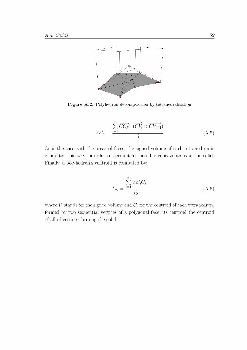
A.4. Solids 69
Figure A.2: Polyhedron decomposition by tetrahedralization
V olS =
n∑i=1
−−→CCF · (
−−→CVi ×
−−−→CVi⊕1)
6(A.5)
As is the case with the areas of faces, the signed volume of each tetrahedron is
computed this way, in order to account for possible concave areas of the solid.
Finally, a polyhedron’s centroid is computed by:
CS =
n∑i=1
V oliCi
VS(A.6)
where Vi stands for the signed volume and Ci for the centroid of each tetrahedron,
formed by two sequential vertices of a polygonal face, its centroid the centroid
of all of vertices forming the solid.
70
Appendix B
Source Code
In the attached CD, the source code of the implemented polyhedral mesh gen-
erator is included, so that it can be further studied, developed and used as a
reference in future work. It should be noted that, as the mesh generator has
been specifically developed for creating meshes usable within DOLFYN open
source CFD analysis code [3], it cannot be considered a generic tool, suitable for
every case where the use of a polyhedral mesh is desired. However, its extension
to supporting more CFD simulation software should be possible, by enriching the
available mesh export options. Additionally, as the present implementation has
been made possible within the environment of the proprietary SOFiSTiK FEA
software [1], it cannot be expected that the source code can be usable without
any modifications, wherever proprietary dependencies may apply. Despite that,
there has been made an effort to keep these dependencies to a minimum level,
with the hope that it will prove a useful point of reference for future studies.
That being said, the included code is provided as is, without warranty of any
kind, and with the permission to study, modify and use for educational purposes.
Contents of the CD:
• Source code of the implemented polyhedral mesh generator
• LATEX source files of the present document
• The present document in PDF format
LIST OF FIGURES 71
List of Figures
1.1 Neighboring elements for triangular and polygonal meshes . . . . 2
1.2 Bounded mesh formed by a Voronoi tessellation . . . . . . . . . . 5
1.3 Mesh formed by a Delaunay triangulation . . . . . . . . . . . . . 6
2.1 Common cases of full mesh representation schemes: explicit adja-
cency information is included for entities of all dimensions . . . . 16
2.2 Common cases of reduced mesh representation schemes: adjacency
information for implicitly represented entities is noted in dashed
objects . . . . . . . . . . . . . . . . . . . . . . . . . . . . . . . . . 17
2.3 Element adjacency templates . . . . . . . . . . . . . . . . . . . . 18
3.1 A primal triangular mesh and its general polygonal dual . . . . . 26
3.2 A primal triangular mesh and its median polygonal dual . . . . . 27
3.3 Generation of internal dual vertices . . . . . . . . . . . . . . . . . 29
3.4 Generation of internal dual edges . . . . . . . . . . . . . . . . . . 31
3.5 Generation of internal dual faces . . . . . . . . . . . . . . . . . . . 32
3.6 Generation of internal dual cells . . . . . . . . . . . . . . . . . . . 33
LIST OF FIGURES 72
3.7 Polyhedral mesh of a complex geometry in 3D . . . . . . . . . . . 34
3.8 Meshing details of a complex geometry in 3D . . . . . . . . . . . . 34
3.9 Volume deflation of ≈ 2.0% due to a curved boundary surface . . 36
3.10 Volume deflation of ≈ 0.5% due to a curved boundary surface . . 36
3.11 Preservation of the geometry of primal mesh surfaces . . . . . . . 36
3.12 Preservation of the geometry of primal mesh edges . . . . . . . . . 37
3.13 Polyhedral mesh with cylindrical hole and internal elliptical void . 39
3.14 Formation of boundary layer with cascading mesh generation in 2D 41
3.15 Formation of boundary layer with cascading mesh generation in 3D 42
4.1 Decomposition of polyhedral cell during the star-shaped test . . . 45
4.2 Cell concavity due to the presence of non-planar faces . . . . . . . 46
4.3 Sections of the interior of 3D meshes generated considering differ-
ent primal cell centers . . . . . . . . . . . . . . . . . . . . . . . . 47
4.4 Location of dual vertices for various cases of primal cell quality . . 48
5.1 Memory requirements for tetrahedral meshes and their polyhedral
counterparts . . . . . . . . . . . . . . . . . . . . . . . . . . . . . . 53
5.2 Polyhedral mesh generation time in comparison with correspond-
ing primal mesh generation . . . . . . . . . . . . . . . . . . . . . . 55
5.3 Unit cube with laminar flow along a main axis . . . . . . . . . . . 56
5.4 Tetrahedral, polyhedral and hexahedral meshing of the 3D domain 57
5.5 Polyhedral mesh generation time in comparison with correspond-
ing primal mesh generation . . . . . . . . . . . . . . . . . . . . . . 58

LIST OF FIGURES 73
5.6 Narrow channel with cylindrical object, with laminar longitudinal
flow . . . . . . . . . . . . . . . . . . . . . . . . . . . . . . . . . . 59
5.7 Details of mesh cases around the cylindrical object . . . . . . . . 60
5.8 Reference results . . . . . . . . . . . . . . . . . . . . . . . . . . . 60
5.9 Contour plots of the velocity vector for increasing mesh refinement
of polyhedral meshes . . . . . . . . . . . . . . . . . . . . . . . . . 61
5.10 Comparative convergence plots for polyhedral meshes of increasing
refinement, as well as for the hexahedral reference mesh . . . . . . 62
A.1 Face decomposition by triangulation . . . . . . . . . . . . . . . . 67
A.2 Polyhedron decomposition by tetrahedralization . . . . . . . . . . 69

LIST OF TABLES 74
List of Tables
2.1 Notation of Adjacency Operators . . . . . . . . . . . . . . . . . . 14
5.1 Number of entities for primal and dual meshes . . . . . . . . . . . 52
5.2 Iterations needed to achieve the same level of convergence . . . . 57
BIBLIOGRAPHY 75
Bibliography
[1] SOFiSTiK AG. http://www.sofistik.com.
[2] Andre Bakker and Elizabeth Marden Marshall. Computational Fluid Dy-
namics, chapter 49, pages 505–515.
[3] DOLFYN Open Source CFD. http://www.dolfyn.net.
[4] Mark de Berg, Otfried Cheong, Marc van Kreveld, and Mark Overmars.
Computational Geometry Algorithms and Applications. Springer, 2008.
[5] Vadim Dyadechko, Rao V Garimella, and Mikhail J Shashkov. Reference ja-
cobian rezoning strategy for arbitrary lagrangian-eulerian methods on poly-
hedral grids. In IMR, pages 459–470. Citeseer, 2004.
[6] JH Ferziger and M Peric. Computational Methods for Fluid Dynamics.
Springer, 3 edition, 2002.
[7] R. V. Garimella. Mesh data structure selection for mesh generation and FEA
applications. International Journal of Numerical Methods in Engineering,
55(4):451–478, October 2002.
[8] R. V. Garimella. Mstk: A flexible infrastructure library for developing
mesh-based applications. In Proceedings of the 13th International Meshing
Roundtable, Williamsburg, VA., 2004.
[9] R. V. Garimella and M. J. Shashkov. Polygonal surface mesh improvement.
Engineering with Computers, 20:265–272, 2004.
[10] Rao V. Garimella, Jibum Kim, and Markus Berndt. Polyhedral mesh gen-
eration and optimization for non-manifold domains. In Josep Sarrate and
BIBLIOGRAPHY 76
Matthew Staten, editors, Proceedings of the 22nd International Meshing
Roundtable, pages 313–330. Springer International Publishing, 2014.
[11] Paul-Louis George and Houman Borouchaki. Delaunay Triangulation and
Meshing - Application to Finite Elements. Editions HERMES, 1998.
[12] J. Gregson, A. Sheffer, and E. Zhang. All-hex mesh generation via volu-
metric polycube deformation. Computer Graphics Forum (Special Issue of
Symposium on Geometry Processing 2011), 30(5):to appear, 2011.
[13] Hrvoje Jasak, Aleksandar Jemcov, and Zeljko Tukovic. Openfoam: A c++
library for complex physics simulations. International Workshop on Cou-
pled Methods in Numerical Dynamics, IUC, Dubrovnik, Croatia, September
2007.
[14] Barry Joe. Shape measures for quadrilaterals, pyramids, wedges, and hex-
ahedra, March 2008.
[15] Michael Kremer, David Bommes, Isaak Lim, and Leif Kobbelt. Advanced
automatic hexahedral mesh generation from surface quad meshes. In
Proceedings of the 22nd International Meshing Roundtable, Berlin, 2013.
Springer-Verlag.
[16] Henk Krus. Dolfyn developers guide, 2010.
[17] H. Ledoux. Computing the 3d voronoi diagram robustly: An easy expla-
nation. In Voronoi Diagrams in Science and Engineering, 2007. ISVD ’07.
4th International Symposium on, pages 117–129, July 2007.
[18] Netgen. Automatic mesh generator. http://sourceforge.net/projects/netgen-
mesher/.
[19] W. Oaks and S. Paoletti. Polyhedral mesh generation. In Proceedings of the
9th International Meshing Roundtable 2000, pages 57–66, 2000.
[20] OpenFOAM. The open source computational fluid dynamics toolbox.
http://www.openfoam.com/.
[21] M. Peric. Flow simulation using control volumes of arbitrary polyhedral
shape. In ERCOFTAC Bulletin, No. 62. September 2004.
BIBLIOGRAPHY 77
[22] M. Peric. Simulation of flows in complex geometries: New meshing and
solution methods. In NAFEMS Seminar: Simulation of Complex Flows
(CFD) – Application and Trends, 2004.
[23] M. Peric and S. Ferguson. The advantage of polyhedral meshes.
http://www.cd-adapco.com/.
[24] Qhull. http://www.qhull.org/.
[25] E. Ruiz-Girones. Automatic Hexahedral Meshing Algorithms: From Struc-
tured to Unstructured Meshes. PhD thesis, Universidad Politecnica de
Cataluna, January 2011.
[26] M. Sato and T. Kobayashi. A fundamental study of the flow past a circular
cylinder using abaqus/cfd. Mechanical Design & Analysis Corporation.
[27] Joachim Schoberl. Netgen an advancing front 2d/3d-mesh generator based
on abstract rules. Computing and visualization in science, 1(1):41–52, 1997.
[28] Martin Spiegel, Thomas Redel, Y Jonathan Zhang, Tobias Struffert,
Joachim Hornegger, Robert G Grossman, Arnd Doerfler, and Christof Kar-
monik. Tetrahedral vs. polyhedral mesh size evaluation on flow velocity and
wall shear stress for cerebral hemodynamic simulation. Computer methods
in biomechanics and biomedical engineering, 14(01):9–22, 2011.
[29] STAR-CCM+. http://www.cd-adapco.com/products/star-ccm.
[30] D. Sunday. Fast polygon area and newell normal computation. Journal of
Graphics Tools, 7(2):9–13, 2002.
[31] TetGen. A quality tetrahedral mesh generator and a 3d delaunay triangu-
lator. http://wias-berlin.de/software/tetgen/.
[32] Visualization Toolkit. http://www.vtk.org/.
[33] D. Vartziotis and B. Himpel. Efficient Mesh Optimization Using the Gradi-
ent Flow of the Mean Volume. ArXiv e-prints, February 2013.
[34] Dimitris Vartziotis and Benjamin Himpel. Efficient and global optimization-
based smoothing methods for mixed-volume meshes. In Josep Sarrate and
BIBLIOGRAPHY 78
Matthew Staten, editors, Proceedings of the 22nd International Meshing
Roundtable, pages 293–311. Springer International Publishing, 2014.
[35] Paraview Open Source Scientific Visualization. http://www.paraview.org/.
[36] Voro++. http://math.lbl.gov/voro++/.
[37] Dong-Ming Yan, Wenping Wang, Bruno Levy, and Yang Liu. Efficient com-
putation of 3d clipped voronoi diagram. Advances in Geometric Modeling
and Processing, pages 269–282, 2010.
[38] Yongjie Zhang, Xinghua Liang, and Guoliang Xu. A robust 2-refinement
algorithm in octree and rhombic dodecahedral tree based all-hexahedral
mesh generation. In Xiangmin Jiao and Jean-Christophe Weill, editors,
Proceedings of the 21st International Meshing Roundtable, pages 155–172.
Springer Berlin Heidelberg, 2013.