1   

 

Pollution, Test Scores and Distribution of Academic Achievement: Evidence

from California Schools 2002-20081

John C. Ham

University of Maryland and National University of Singapore, IFAU, IFS, IRP (UW-Madison) and IZA

Jacqueline S. Zweig

Economics University of Southern California

Edward Avol

Keck School of Medicine University of Southern California

Revised February 2014

 

                                                            1 Ham is corresponding author (john.ham.econ@gmail.com). Ham’s work was supported by NSF grant SBS0627934. We are grateful for helpful comments from Timothy Moore, M. Pastor, Geert Ridder and especially Serkan Ozbeklik gave us very useful suggestions. Particularly helpful comments from two anonymous referees and the Co-Editor drastically improved the paper. Any opinions, findings, and conclusions or recommendations in this material are those of the authors and do not necessarily reflect the views of the National Science Foundation. We are responsible for any errors.

2   

 

Abstract

One of the main arguments in favor of stricter regulations on air pollution is that it has harmful effects on

child and adult health. Air pollution is associated with asthma, lower lung function, hay fever, infant

mortality, and emergency room visits. Moreover, economists and epidemiologists also have found that

increased air pollution increases school absenteeism, and that asthma may reduce school performance. If air

pollution negatively affects children’s health and increases school absenteeism, it is plausible that it would

negatively affect their educational attainment. Given the strong (heavily documented) relationship between

academic performance and future labor earnings, this negative relationship suggests a heretofore

unappreciated additional cost of air pollution in terms of reduced future earnings. Further, since low-income

children tend to live in high pollution areas, reducing pollution may decrease income inequality and increase

social mobility.

We first use regression analysis to examine the effect of changes in air pollution on the performance

of 2nd through 6th grade students in California on standardized tests. Specifically, our four outcomes of

interest are the mean scaled score and the percent of students at least proficient in both Mathematics and in

English/Language Arts at the grade-school level. Our measures of pollution are carbon monoxide, nitrogen

dioxide, ozone, coarse particulate matter, and fine particulate matter. We use grade-school FEs and a large

number of time changing control variables in our analysis. Secondly, we examine the effect of an additional

unit of pollution on different quantiles of the educational achievement distribution of these four performance

measures using FE quantile regression analysis.

We find that a one standard deviation reduction in ozone, fine particulate matter, and especially

coarse particulate matter generally increases these four performance measures at the mean and at the different

quantiles by a small, but statistically significant, amount. A one standard deviation in nitrogen dioxide has a

small but significant effect only on Mathematics scores, while in the vast majority of cases, the carbon

monoxide coefficients are insignificant. These results are robust to a number of changes in how pollution is

measured. In terms of comparing the quantile and regression estimates, the median estimates are similar to,

but generally slightly more significant than, the FE regression results. In many cases, if the quantile estimates

are significant for some quantiles, they are statistically significant for all quantiles. In a slight majority of cases

where the pollutant has a significant coefficient in the quantile estimates, the effect increases across quantiles,

while in the other cases the coefficient for a given pollutant is constant across quantiles.  

3   

 

1. Introduction

The effects of air pollution on child and adult health have been widely studied. In fact, one of the

main arguments in favor of stricter regulations on air pollution is that it has harmful effects on child

and adult health. Air pollution is associated with asthma, lower lung function, hay fever, infant

mortality, and emergency room visits (Chay and Greenstone, 2003ab; Currie and Neidell, 2005,

Gauderman et al., 2000; McConnell et al., 2002; McConnell et al., 2003; Neidell, 2004; and

Rabinovitch, Strand, and Gelfand, 2006). Moreover, economists and epidemiologists have found

that increased air pollution also increases school absenteeism (Currie, Hanushek, Kahn, Neidell, and

Rivkin, 2009; Gilliland et al., 2001; Ransom and Pope, 1992), and that asthma may reduce school

performance (Currie, Stabile, Manivong, and Roos, 2010).

If air pollution negatively affects children’s health and increases school absenteeism, it is

plausible that these children’s educational attainment would also be negatively affected. Given the

strong relationship between academic performance and future labor income, a negative effect of

pollution on educational attainment suggests a heretofore unappreciated additional cost of air

pollution in terms of reduced future earnings. Further, pollution may also have different effects

across the income distribution; for example, if another unit of pollution negatively affects

disproportionately the lower quantiles of the academic distribution, it will disproportionately affect

the achievement of low-income children, given the strong relationship between children’s academic

achievement and family background. Further, even if these effects are constant across the

achievement distribution, low-income children will be disproportionately affected because low-

income households disproportionately live in more highly polluted areas. Thus, an additional unit of

overall pollution may increase income inequality and social mobility.

The central difficulty in identifying the effects of air pollution on academic performance is

that air pollution is likely to be correlated with socioeconomic status; as noted above, higher income

families are likely to sort into lower-pollution neighborhoods. Because children from lower income

families tend to have lower test scores than those from higher income families, a finding of a

negative effect of pollution on test scores may simply reflect selection. Of course, this problem is

not unique to our paper: all papers in the economics literature attempt to eliminate the confounding

factor of socioeconomic status when estimating the effect of pollution on an outcome variable.

4   

 

Many of these articles use appropriate conditioning variables and fixed effects (hereafter FEs). Some

studies aim to reduce this selection problem by using variation across time intervals that presumably

are too short to reflect location behavior, albeit at the cost of making the assumption that variables

outside this short time interval do not affect the outcome of interest.

In this paper we follow the first strategy described above and use appropriate FEs to control

for selection when investigating the effect of pollution on academic achievement. First, we examine

the effect of changes in air pollution on the mean academic performance of school children in

California, using standard FE regression analysis. Second, we examine the effect of an additional

unit of pollution on different quantiles of the educational achievement distribution, using FE

quantile regression analysis. Quantile regression analysis has been sparingly used to study the effect

of pollution; one obvious explanation for its infrequent use is that, up until recently, it has not been

possible to incorporate FEs into this framework due to the standard incidental parameters problem

that arises when one uses fixed effects with a nonlinear estimator. Canay (2011) presents a feasible

means of using FEs in this framework, and we exploit his work in this paper.

We use the results of the California Standards Tests in Mathematics (hereafter Math) and

English/Language Arts (hereafter ELA) as measures of academic performance (California

Department of Education, 2002-2008c). Specifically, our four outcomes of interest are the mean

scaled score and percent of students at least proficient in Math and in ELA at the grade-school level.

Our pollution variables are the percent of days above the standard for carbon monoxide (CO),

nitrogen dioxide (NO2), ozone (O3), coarse particulate matter (PM10), and fine particulate matter

(PM2.5). We calculate the pollution measures for each school in California from all monitors

(weighted by distance from the school) within a twenty mile radius of the school. Our sample is

limited to the years 2002 to 2008 because that is the period during which the content of the tests

remained constant. We use an average of the daily pollution levels for September through May. We

also consider the sensitivity of our results to different ways of measuring pollution and find that our

original results are generally robust to such changes.

To avoid the problem of confounding factors or selection biasing our results, we include

grade-school FEs, year effects, as well as a host of time-varying school quality, demographic, and

community characteristics in the regressions. Thus, this paper makes two important contributions to

the pollution literature. We are the first to estimate what economists view as the causal effect of

5   

 

pollution on the mean of measures of academic performance at the grade-school level. Moreover,

we are the first to exploit Canay’s (2011) results and look at the effect of pollution on different

quantiles of the outcome of interest after controlling for appropriate FEs.

The paper proceeds as follows. We review the relevant literature in section 2. We first

discuss the economics literature to date on the related topics of the effect of pollution on health, the

effect of pollution on school absenteeism, and the effect of asthma, which is exacerbated by and

possibly caused by pollution, on academic performance. Next, we review work from the public

health literature concerning the above issues as well as examining correlations between pollution and

test scores. We conclude that because the epidemiological literature is based on cross-section data, it

is unlikely that economists would consider the estimated effects as causal. In section 3 we outline

our econometric approach and discuss our identification strategy. We describe the data in section 4.

We present our results in section 5, where we measure (separately) the effects of five

pollutants on four measures of academic performance: i) mean Math scores; ii) the percent of

students at least proficient in Math; iii) mean ELA scores; and iv) the percent of students at least

proficient in ELA. In terms of statistical significance, the effects are strongest for O3, PM2.5, and

especially PM10. NO3 significantly affects only the Math outcome variables, while in the vast majority

of cases, the CO coefficients are insignificant. However, all of the pollution effects we measure are

relatively small. The above results are robust to a number of changes in how pollution is measured.

In terms of comparing the quantile and regression estimates, the median estimates are similar

to, but generally a bit more significant than, the regression results. In many cases, if the quantile

estimates are significant for some quantiles, they are statistically significant for all quantiles. In a

slight majority of cases where the pollutant has a significant coefficient in the quantile estimates, the

effect increases across quantiles, while in the other cases the coefficient for a given pollutant is

constant across quantiles. Again, the estimated effects of the different forms of pollution are small.

We carry out comparative static results concerning the effect of changing pollution levels on the

difference between high and low-income students, and high achievement and low achievement

students. Section 6 concludes the paper.  

6   

 

2. Literature Review

Pollution can affect academic performance by way of three mechanisms: (i) school absenteeism due

to illness caused by pollution; (ii) attention problems in school due to illness caused by pollution; (iii)

fatigue when doing homework due to illness caused by pollution, and (iv) a direct negative effect of

pollution on brain development. All of the research on (iv) is drawn from epidemiological and

neuropathology research; thus, we discuss it in section 2.2, which reviews such research.

2.1 Mechanisms by Which Pollution Can Affect Academic Performance–Evidence from the Economics Literature 

Mechanisms (i)-(iii) above rely on pollution having a negative effect on health, and then health

impacting students’ academic performance. In this subsection, we highlight some of the economics

articles investigating these mechanisms.2 Chay and Greenstone (2003ab) examine the effect of air

pollution on infant mortality rates in United States counties between 1980 and 1982. Their initial

identification strategy is based on assuming that county FEs, state trends, year effects, and

socioeconomic controls are sufficient to eliminate most spurious correlations between pollution and

infant mortality. Their socioeconomic controls include mother-specific characteristics aggregated to

the county-level, including education, ethnicity, income, prenatal care, and age. They chose the

period from 1980 to 1982 with the belief that/on the assumption that that much of the remaining

variation in pollution after controlling for these variables comes from the differential impacts of the

1980 recession on pollution levels. Therefore, they argue, changes in pollution are transitory and less

likely to affect location choice. One caveat to this identification strategy is that one must ignore the

fact that the recession will also directly affect location decisions as adults move from hard-hit labor

markets to more prosperous labor markets, i.e. there may still be selection at work.

  Chay and Greenstone weaken their identifying assumptions in several ways. First, they treat

current pollution as endogenous, instrumenting for the change in pollution with lagged pollution

levels; the latter will be a valid instrumental variable (IV) if there is no autocorrelation in pollution.

                                                            2 Several articles outside the economics literature establish this link as well (see McConnell et al., 2002, Gauderman et al., 2000, and McConnell et al., 2003); however, for brevity, we focus on the economics papers.

7   

 

Second, they group the treatment and control counties based on the size of income changes between

1980 and 1982 and use their first differences estimation strategy. Finally, they restrict the sample to

counties with low manufacturing employment. They compare changes in infant mortality rates

across low manufacturing counties that bordered a county with high manufacturing employment in

1980 to those counties that bordered other low manufacturing counties. In the former case, a

substantial decrease in a neighboring county’s manufacturing employment is likely to cause a

reduction in Total Suspended Particles (TSPs) in the county of interest because of wind and other

weather components. Thus, their new identifying assumption is that demand shocks in a

neighboring county will not have spillover effects that induce migration from the county under

consideration. 

Neidell (2004) evaluates how seasonal changes in pollution affect asthma-related hospital

admission rates for different age groups by month, conditional on zip code-year FEs and year-

month FEs. For each zip code, he constructs a monthly measure of pollution by taking the average

of pollution levels recorded at monitors within 20 miles of the centroid of the zip code weighted by

the inverse distance to the monitor. The outcome variable is the number of asthma-related

emergency room visits in each zip code-month observation, where a visit is classified as asthma-

related based on the principle diagnosis from the California Hospital Discharge Data. The control

variables include the sex, race, and age of the patient, expected source of payment to the hospital,

weather, and housing prices. Neidell finds that, of the pollutants considered, carbon monoxide has a

significant effect on hospitalizations for asthma among children ages 1–18, while none of the

pollutants considered has a clear impact on hospitalizations for infants. Using estimated coefficients

and the expected number of asthma admissions from 1992 and 1998 pollution levels, Neidell

calculates that the decline in pollution during this time period caused asthma admission rates to

decrease from 13.5% to 4.6%. Neidell also tests, by including the number of smog alerts as a

control variable, whether families display avoidance behavior. He concludes that they do exhibit

avoidance behavior; the smog alert coefficient is negative and significant, while the magnitude of the

negative coefficient on O3 is smaller when smog alerts are included in the regressions. Because he

uses a large number of FEs, the only caveat to Neidell’s results is that he must assume that pollution

in previous months does not affect admissions in subsequent months; this assumption would be

8   

 

violated if previous pollution caused individuals to develop asthma, which made them more sensitive

to current pollution. While of course this criticism could also be leveled at studies using annual data

(as in the consumer demand literature), it is likely that this type of separability over time periods is

less credible as the size of the period decreases.

Currie and Neidell (2005) evaluate the effect of increased air pollution on infant mortality

during the period from 1989 to 2000. The authors construct a weekly pollution measure similar to

that in Neidell (2004) by taking the average of pollution levels recorded at monitors within 20 miles

from of centroid of the zip code weighted by the inverse distance to the monitor. The authors

include zip code month FEs and zip code year FEs. The authors include various mother-specific

factors, including mother’s age, race, ethnicity, education, marital status, zip code of maternal

residence, use of prenatal care, and private/public insurance. Other covariates include weekly

county-level averages for weather, date of birth, birth weight and gestation period. They use a

flexible discreet hazard model where the outcome variable is equal to one if the child died within the

week. They find that, in periods of higher pollution, although infant mortality rates are higher,

prenatal exposure to pollution does not affect infant mortality. They often find that ozone has the

incorrect sign, but attribute this finding to a negative correlation between ozone and other

pollutants. We offer two criticisms of their work. First, they must assume that there is no

unobserved heterogeneity at the individual or zip code level, since either form of heterogeneity will

cause their parameter estimates to be biased. Second, they must assume that, conditional on duration

(of life), pollution levels of previous periods do not affect mortality.

Currie et al. (2009) investigate the effect of pollution on school absences, using data from

the Texas Schools Project, a longitudinal administrative data set on student absenteeism in Texas.

They aggregate pollution data from the Texas Commission on Environmental Quality into six-week

time blocks, and merge these data with the administrative absenteeism data. Their identification

comes from the variation in pollution across six-week attendance periods within a year or within an

attendance period across years. In the former case, they include school by attendance period FEs; in

the latter case, they include school by year FEs. They measure pollution by determining whether

each day is 0-25%, 25-50%, 50-75%, 75-100% or greater than 100% of the relevant Environmental

Protection Agency (EPA) threshold for a particular pollutant. They then calculate the shares of days

in each category for the six-week attendance period. Their main finding is that CO between 75-

9   

 

100% of the air quality standards threshold and above the threshold has a positive and significant

effect on school absences. Ozone is not statistically significant in most specifications, but they did

find a statistically significant increase in absences associated with PM10 levels between 50-75% of the

EPA threshold. This latter result is somewhat surprising since in this case one would also expect

pollution levels between 75% to 100% of the threshold, and above the threshold, to matter; of

course, it may be that the effects of the higher levels of pollution simply have large confidence

intervals. Indeed, as the authors acknowledge, the result of a significant effect for PM10 levels

between 50-75% of the threshold must be viewed with caution, since one significant result among

many coefficients can occur by chance. Again, the identifying assumption in their work is that past

pollution levels do not affect current absences; as noted above, this assumption would be violated if

previous pollution levels increased the incidence of asthma, which in turn accentuated the effects of

pollution in the current period.

Of course, air pollution affects academic performance through health only if health

problems affect performance. Currie et al. (2010) evaluate the effect of various childhood diseases,

including asthma, on (i) how students performed on a literacy exam, (ii) whether the students

enrolled in a college preparatory math class, (iii) whether they were in the twelfth grade by age 17,

and (iv) whether they used social assistance. They match school administrative data, social assistance

records, and health records for young adults in Manitoba, Canada born between 1979 and 1987.

With a mother FE (which controls for time constant family characteristics), they investigate whether

having been treated for asthma at various ages (0-3, 4-8, 9-13, 14-18) affects these young adult

outcomes by using the variation across siblings in the incidence of asthma. They find (at the 10%

level) that (a) asthma at ages 9 to 13 had a significant negative effect on taking a college preparatory

math class and (b) asthma at ages 14 to 18 sometimes had a negative effect on the literacy score in

the 12th grade. They find no effect of earlier asthma, conditional on current asthma. As the authors

acknowledge, their results must be viewed with caution since, again, two significant coefficients

could happen by chance in this framework. Their identifying assumption is that there are no time

varying family characteristics, i.e., socioeconomic status, that would be correlated with both asthma

and these outcome variables, and that the asthma effect does not pick up the effect of current

pollution.

10   

 

2.2 Mechanisms by Which Pollution Can Affect Academic Performance–Evidence from the Epidemiological Literature

All of the studies from the epidemiological literature are based on cross-section data and use a

relatively small number of controls. As a result, these researchers are much more limited in their

ability to deal with selection and endogeneity issues than would be standard in health economics;

indeed, this latter problem is accentuated by the fact that none consider instrumental variable

estimation.

Gilliland et al. (2001) use the Children’s Health Study data to evaluate the effect of pollution

on absenteeism. They study a cohort of 2,081 4th grade students who reside in 12 southern California

communities. They track the students’ absences for the first 6 months of 1996, following up with

the students’ parents to determine whether the absence is illness-related or not, and if so, whether it

is an upper-respiratory, lower-respiratory, or gastro-intestinal illness. The type of illness is

determined by the symptoms described during phone interviews with a family member. Using daily

pollution levels from monitors located near the schools and a community FE model, the authors use

within-community variation in pollution across the six-month period to determine its effect on

average daily absences due to respiratory illness. They find that ozone has a statistically significant

relationship (partial correlation) with reported absences from upper-respiratory and lower-

respiratory illness rates. To obtain a causal effect, they need to assume that, within a community,

families do not sort themselves based on permanent differences in pollution across the community.

We now consider a number of other studies that use cross-section data and no FEs,

rendering them less credible in terms of estimating causal effects. Fowler, Davenport, and Garg

(1992) analyze the effect of asthma on different outcomes for the United States. They use data for

10,362 children in 1st through 12th grade from the 1988 United States National Health Interview

Survey. They find that children with asthma are more likely to have a learning disability than children

who do not have asthma. In addition, among households with incomes below $20,000, asthmatic

children are twice as likely to fail a grade as those without asthma. However, among higher income

families, asthmatic children have only a slightly higher failure rate than non-asthmatic children.3 With

a sample of 1,058 kindergarten-age children from Rochester, New York in 1998, Halterman et al.                                                             3 This finding suggests the possibility of heterogeneous asthma effects by socioeconomic status, but we felt that we did not have sufficient data to explore this possibility in our analysis.

11   

 

(2001) compare the parent-reported development skills of asthmatic children to those of non-

asthmatic children. After controlling for type of health insurance, education of the care-giver,

gender, and pre-kindergarten education, the authors find that asthmatic kindergarten-aged children

scored lower in school readiness skills (one category of reported development skills) than their non-

asthmatic peers. Butz et al. (1995) obtain demographic asthma symptoms and psychosocial

information for 392 children in kindergarten through 8th grade in 42 schools in Baltimore, Maryland.

Asthma symptoms are divided into low, medium, and high levels. A child is considered to exhibit

behavioral problems if her score on a questionnaire containing standardized psychosocial questions

is higher than a given threshold. Using logistic regressions, the authors conclude that parents who

report that their children have higher levels of asthma symptoms are twice as likely to report a

behavioral problem compared to parents who report lower levels of asthma symptoms.

Bussing, Halfon, Benjamin, and Wells (1995) first use responses to the 1988 National Health

Interview Survey on Child Health to categorize children into those who suffer from asthma alone,

those who suffer from asthma combined with other chronic conditions, those who suffer from

other chronic conditions alone, or those who have no chronic (including asthmatic) conditions.

They then combine this information with a Behavior Problem Index constructed from psychosocial

questions in the NHI survey. Using logistic regressions, the authors find that children with severe

asthma alone are nearly three times as likely to have severe behavioral problems as children without

a chronic condition. Halterman et al. (2006) investigate the relationship between behavioral

problems and asthma symptoms for a cohort of 1,619 inner-city students in Rochester, New York.

The parents of these kindergarten-age children were surveyed about their children’s health and

behavior. The authors find that children with persistent asthma score worse on peer interactions and

task orientation, and are more likely to exhibit shy and anxious behaviors compared to non-

asthmatic children.4

Epidemiologic, neuropathological, and brain imaging studies also provide evidence of a

negative relationship between ambient air pollution and brain development conditional on                                                             4 According to the National Heart, Blood and Lung Institute of the National Institutes of Health (2007, p. 72), asthma is considered persistent if the patient experiences symptoms more than two days per week, limitation in activities, some nighttime awakenings or use of short acting beta2 agonists combined with either more than two exacerbations requiring oral steroids or more than four wheezing episodes longer lasting than a day per year.

12   

 

observable demographic factors. Among 202 children who were approximately 10 years old in

Boston, Massachusetts, higher levels of black carbon (a marker for traffic particles) were associated

with decreased cognitive function across assessments of verbal and nonverbal intelligence and

memory constructs (Suglia et al. 2008). The authors estimate exposure to black carbon for each

participant’s current residence and control for age, gender, mother’s education, and language spoken

at home. In a prospective study of a birth cohort of 249 children whose mothers lived in New

York’s Harlem and South Bronx areas during pregnancy, Perera et al. (2009) investigate the effect

of polycyclic aromatic hydrocarbons (PAHs) on a child's intelligence quotient (IQ).5 Motor vehicles

are a major source of PAH in Harlem and the South Bronx. PAH levels are measured through

personal monitoring of the mothers in their third trimester of pregnancy; IQ was evaluated using the

Wechsler Preschool and Primary Scale of Intelligence-revised. The researchers find that children

with prenatal exposure to high levels of PAHs have full scale and verbal IQ scores at age 5 that are

4.31 and 4.67 points lower, respectively, than those of less exposed children. In a cross-sectional

study in Quanzhou, China, Wang et al. (2009) find that 8- to 10-year-old children attending a school

located in a high traffic exhausts pollution area perform worse on multiple neurobehavioral function

tests compared to those studying at another school, located in a clean air area. The authors chose

the schools based on traffic density and air pollution monitoring data, and they control for, among

other things, father’s education, age, sex, birth weight, and second-hand smoke.

Calderón-Garcidueñas et al. (2008a, 2008b) led a series of clinical, neuropathological, and

neuroimaging studies on clinically healthy and neurocognitively intact children and adolescents

growing up either in Mexico City (a place with high ambient air pollution) or in clean air areas. In

Calderón-Garcidueñas et al. (2008a), the authors find that among the forty-seven subjects who died

suddenly, accumulations of amyloid β42 (a marker of neurodegenerative disease) in the prefrontal

brain region and disruption of the blood-brain-barrier were observed in the lifetime residents of

Mexico City (n=35) but not in the comparison group (n=12). 6 In another study, Calderón-

Garcidueñas et al. 2008b find that children from Mexico City exhibit significant deficits in a

                                                            5 Polycyclic aromatic hydrocarbons are formed by incomplete combustion of fossil fuels, among other organic material. Prenatal exposure to PAH has been linked with adverse immune, metabolic, and neurological functions and reduced birth weight. 6 The comparison group consisted of residents of Tlaxcala and Veracruz.

13   

 

combination of fluid and crystallized cognition tasks, as compared to other children from Polotitlán,

a selected clean-air city. Fluid cognition is supported by working memory, while crystallized

cognition is supported by long-term memory. The 55 subjects from Mexico City and the 18 subjects

from Polotitlán cities were from middle-class families. Their mothers had similar average years of

formal schooling groups, and their households had a bedroom separate from the kitchen. Brain

MRI-measured hyperintense white matter lesions substantially increased in children from Mexico

City (56.5% vs. 7.6% in the control city). White matter lesions may affect cognitive dysfunction, and

particulate matter may contribute to neuroinflammation.

Pastor, Sadd, and Morello-Frosch (2004) evaluate the relationship between academic

performance and environmental hazards in the Los Angeles Unified School District in 1999. They

combine data on schools’ Academic Progress Index (API) with information on their proximity to

Toxic Release Inventory (TRI) emissions and census tract-level estimated respiratory risks associated

with concentrations of 148 ambient air toxins. This latter measure of exposure at the tract level is

the sum of hazard ratios for each pollutant, where the hazard ratio is calculated by dividing the

EPA’s tract-level exposure estimate for a particular pollutant by the amount of toxicant below which

there should be no adverse health effects. According to the California Department of Education

(2010, p. 6), the API “is calculated by converting a student’s performance on statewide assessments

across multiple content areas into points on the API scale. These points are then averaged across all

students and all tests.” Each school receives one API score. In an OLS regression, the authors

regress the API score on the respiratory risk index, a dummy equal to one if a facility releasing

substances covered by the TRI and in the 33/50 program is within one mile of the school.7 The

authors find that having a 33/50 facility within a one-mile radius has a negative and significant effect

on academic performance, even after controlling for socioeconomic status variables such as parents’

education, percent minority, and percent who are English learners.

Finally Pastor, Morello-Frosch, and Sadd (2006) expand their previous analysis to all schools

in California. They again use the API score as their measure of academic performance and construct

similar respiratory risk indices. To examine whether the mechanism by which exposure to air

                                                            7 The 33/50 program was a voluntary program by the EPA established to reduce the release of 17 targeted priority chemicals. Enacted in 1991, its goals were to reduce the release and transfer of chemicals by 50% by 1995, as measured against a 1988 baseline (EPA, 1999).

14   

 

pollution affects academic performance is through asthma, the authors first run a Tobit regression

of the three-year averaged, age-adjusted, asthma hospitalization rates by Zip Code Tabulation Area

on their measure of exposure controlling for socioeconomic status. They find that areas with higher

respiratory risk have higher hospitalization rates. They then turn to academic performance, and

find, again, that schools located in higher pollution areas have lower API scores. They estimate that

moving from the seventy-fifth quantile to the median level of the respiratory hazard ratio would

improve test scores by about 1.2%. However, the assumptions necessary to interpret their estimates

of the effect of pollution on school performance as causal are identical to the epidemiological

studies discussed above and hence likely to be much too strong. In the section below, we aim to use

an econometric approach very similar to those used in the economics papers discussed above so that

our estimates of the effect of pollution on school performance can be credibly viewed as causal.

3. Empirical Strategy 3.1 Estimating Pollution Effects Using A Fixed Effect Regression Model

Our data, described in detail below, consists of approximately 24,000 grade-school units observed

for up to seven years. Given that we have panel data, our first empirical specification for our

outcome of interest, ,gstS which represents a measure of performance on a given standardized test

for grade g in school s (located in county c) in year t, is given by

where stP represents pollution at school s at time t, gstX represents the racial composition in grade g

at school s at time t, stW represents school specific characteristics for school s at time t, ctZ

represent time-changing county level factors, gsf represents school-grade FEs, tD represents a full

set of time dummies, and gst is the error term.

As noted above, being able to account for confounding factors is crucial to the credibility of

our analysis (or any such analysis). To account for these factors, in addition to grade-school FEs and

year effects, we first use students’ ethnicity from the California Basic Educational System Data

, 1 2 3 4 (1)gstgst st gst st ct gs tS P X W Z f D

15   

 

(California Department of Education, 2002-2008b) as a control variable. Our other educational

controls are from the Academic Performance Index (API) data files (California Department of

Education, 2002-2008a). We first condition on average class size, which is measured separately for

grades 4 through 6 and kindergarten through grade 3. We also control for the following variables at

the school-year level: the percent of students receiving free or reduced-price lunches; the educational

make-up of parents; the percent of students who are native English speakers; the percent of teachers

who are fully certified; and total enrollment. In addition, we control for annual expenditure per

student at the district level using data from the National Center for Education Statistics’ Common

Core of Data (2002-2008).8 Finally, we control for a number of business cycle variables at the county

level: unemployment rate and taxable transactions (the lowest level of geographical aggregation

available). We adjust taxable transactions and expenditures per student for inflation.

Thus, our identification comes from assuming that all the variation in pollution over time at

a specific school, after controlling for , , gst st ctX W Z and year dummies tD , is uncorrelated with any

remaining unobservables driving school performance. We argue that our rich set of FEs and control

variables renders our identifying assumptions on a par with those made in the economic studies

discussed above. Finally, we make the standard GLS (heteroskedasticity) adjustment of weighting

observations by the respective square root of the number of students in the grade-school-year

observation. However, to allow for autocorrelation over time and any other sources of

heteroskedasticity, the standard errors are still clustered at the school level.

3.2 Estimating Pollution Effects Using a Fixed Effect Quantile Regression Model

In the previous section we presented our strategy for identifying the effect of pollution on mean test

scores. In this section we consider pollution’s effect on test scores at other points in the distribution.

We use the following equation for the th quantile of the distribution for an outcome of interest:

1 2 3 4 5( ) ( ) ( ) ( ) ( ) ( ) ( ) , (2)gst gst gst st ct gs t tt

Quant S P X W Z f D

                                                            8 Because we include a full set of time dummies, all monetary quantities can be interpreted as measured in real dollars.

16   

 

where ( )gsf is a quantile specific FE for grade g in school s, and the other variables are defined

below equation (1)9. (Our parameters of interest are the coefficients 1( ) .)10 In other words, if

grade g in school s is in quantile , its achievement consists of its quantile-specific fixed effect and

the quantile-specific (other) coefficients times their respective time-changing characteristics

(including pollution). Note that this is an extremely rich specification because it involves estimating a

fixed effect for grade g in school s for every quantile, even for quantiles where it is never observed;

not surprisingly, we cannot consistently estimate (2) as specified. This is an important problem

given our claim above that including FEs is crucial for obtaining estimates of the causal effect of

pollution on academic performance. However, Canay (2011) provides an intuitive solution to this

problem, which allows for consistent estimation of a FE quantile model – to assume that the FEs

are constant across quantiles for grade g in school s 11

1 2 3 4 5( ) ( ) ( ) ( ) ( ) ( ) ( ) , (3)gst gst gst st ct gs t tt

Quant S P X W Z f D

This specification has a natural intuitive interpretation – the achievement of grade g in school s if it

in quantile in year t is the sum of its fixed effect plus the quantile specific coefficients times its

time-changing characteristics. Using this assumption, Canay shows that the first step is to run the

standard FEs regression model (1), and solve for the least squares estimates of the FEs. Next, one

subtracts the estimated FEs from the respective outcome variables to obtain new outcome variables.

Finally, one uses standard quantile regression using these new outcome variables. There still remains

the problem of calculating standard errors for the parameter estimates when we assume that

observations in the same school are correlated in a given year and across years. We use the bootstrap

to calculate these standard errors.

                                                            9 A very accessible treatment of quantile regression is presented in Imbens and Wooldridge (2008). They also provide the assumptions necessary for quantile regression to produce interesting results. 10 Consider the median for a symmetric distribution, since in that case the mean and median are equal, and

1( ) for the median will equal (in an expected value sense) the regression coefficient on pollution 1 from

equation (1).

11 That is, *( )gs gsf f for all .

17   

 

While necessary for estimation, the common fixed effect assumption across quantiles may be

considered too strong. To shed some light on this issue, we note that if the outcome variables have a

symmetric distribution, the mean and median will be equal for such a distribution. Since linear

regression allows the mean to have its own FE, while the quantile analysis for the median assumes a

constant FE across quantiles, if the coefficients from the linear regression and median regression

are similar, this would suggest that the quantile estimates are not unduly affected by the common FE

assumption.12

4. Data, Variable Definitions, and Summary Statistics

The summary statistics for the variables used in this study are shown in Table 1. Panel A contains

summary statistics for our OLS outcome variables at the grade-school-year level; here, for both

Math and ELA we use the i) mean scaled score and ii) the percentage at least proficient. The average

scaled scores for Math and ELA are 358 and 341 respectively, while the average percentage at least

proficient for and ELA are 50.8% and 43.5% respectively. (The goal in California is for all students

to score at least proficient; a student with a scaled score above 350 out of 600 is considered at least

proficient.) We include only data on years 2002 through 2008 because the test format changes

outside this time interval. Our analysis includes grades 2 through 6 because the same tests are

administered to all students within each grade. We do not use data from grade 7 on because at that

point students may take different mathematics courses based on ability – for example, algebra,

geometry, or basic math – which would raise difficult selection issues for our analysis.

As noted above, we focus on the coefficients for five pollution variables: coarse particulate

matter (PM10), fine particulate matter (PM2.5), nitrogen dioxide (NO2), carbon monoxide (CO), and

Ozone (O3). We use these specific pollutants in our analysis because they have been studied in the

previous literature (Currie et al., 2009, Gilliland et al., 2001) and are correlated with various diseases

(Gauderman et al., 2005; Grahame and Schlesinger, 2007; Kurt, Mogielnicki, Chandler, 1978; Linn,

Szlachcic, Gong, Kinney, and Berhane, 2000; McConnell et al., 2002, Pope and Dockery, 2006;

Russell and Brunekreef, 2009; and Yu, Sheppard, Lumley, Koenig, and Shapiro, 2000). Vehicle

                                                            12 Of course, the contrary is not true – the mean and median coefficients may be different because the distribution is not symmetric or the common FE assumption is inappropriate.

18   

 

exhaust is a major source of PM10, PM2.5, NO2, and CO. Other sources of particulate matter include

dust from the earth's surface, pollen, forest fires, power plants, and factories. The greatest exposure

to CO comes from smoking cigarettes, but it is also formed through the improper burning of

various fuels. NO2 is emitted from coal-burning power plants and the burning of fossil fuels. O3 is

formed through a chemical reaction between nitrogen oxides, sunlight, and various gaseous

pollutants, which are often emitted from vehicles.13

Pollution data are from the Air Resources Board of California, (Daily Data, 2010). The only

feasible way of measuring pollution is at the school-year level, as we do not have access to students’

addresses. (Thus, there is no variation in pollution across grades for a given school in a specific

year.) The pollution measure used in this study is the percent of days that exceed the California

Standard for that pollutant. The California one-hour standards are 20 parts per million (ppm) for

CO, 0.18 ppm for NO2, and 0.09 ppm for O3. The standards for PM10 and PM2.5 are based on a 24-

hour measure rather than a one-hour measure. The 24-hour standard is 50 3/g m for PM10 and 35 3/g m for PM2.5 (California Environmental Protection Agency, 2009). The California standards are

stricter than the federal standards for all pollutants except for PM2.5, which is the same as the federal

standard.

To obtain our pollution measures, we first use the longitude and latitude of each school and

of each pollution monitor in California to find all monitors within a 20-mile radius of each school.

For a given pollutant and monitor, we calculate the total number of days that exceed the standards

for that pollutant and then divide by the total number of days that are tested. Since students usually

take the California Standards Tests in April or May, we use pollution data from September through

May as an approximation of the pollution experienced during the school year. Then, for a given

pollutant at a given school in a given year, we take the weighted average of the percent of days

exceeding the standard at each monitor, where the weighting is based on the inverse distance to the

school. Thus, we give monitors that are closer to the school more weight relative to ones that are

further away. However, we also consider results based a number of alternative means of measuring

pollution at the school levels. We present the results of this exercise below, and find that our results

are robust to these changes.

                                                            13 For additional information on these pollutants, see Environmental Protection Agency (2011).

19   

 

The summary statistics for our pollution variables are shown in Panel B of Table 1. In Table

2 we show the correlation matrix for the pollution variables. Table 1 indicates that an average of

0.0039%, 0.0033%, 1.94%, 11.78%, and 6.45% days of the school year are above the California

standards for CO, NO2, O3, PM10, and PM2.5. The correlation matrix in Table 2 indicates that some

of the pollution measures are highly correlated.14 This latter result suggests that simultaneously

using the different pollution measures is likely to cause a serious multicollinearity problem among at

least some of the pollution measures; thus, we follow the literature and enter them one at a time.

We also include the control variables outlined in the previous section. The summary statistics

for these are presented in Panel C of Table 1. In terms of ethnic composition of the students, on

average 35.0% of the students are White, 11.0% are Asian, 42.6% are Hispanic, 7.6% are African

American, and 3.8% are other ethnicities. The average class size is 26.5 students, and 94.7% of all

teachers are fully certified. Further, on average, 51.4% of students receive a free or reduced-price

lunch, and the percent of students who are non-native English speakers is 26.2%. The average

enrollment and real expenditure per student are 406.9 and $8,828, respectively. The average county

unemployment rate is 6.3%, and the average real value of county taxable transactions is

approximately $384 million. Unlike some other studies, we did not include weather as a conditioning

variable since it is difficult to obtain a meaningful measure of weather at an annual level. Further,

Morretti and Neidell (2009) show that including weather does not affect estimates of the impact of

ozone on health.

5. Empirical Results 5.1 Main Fixed Effect Linear Regression Results

In Table 3A we show the estimated effects of pollution on mean scaled Math scores from the

standard FE linear regression model. In column (1), our pollution measure is the percent of days

above the standard for carbon monoxide (CO). In columns (2)-(5), we include (separately) the

percent of days above the standard for nitrogen dioxide  (NO2), ozone (O3), coarse particulate matter

                                                            

14 PM10 and PM2.5 are particularly highly correlated, while O3 is essentially uncorrelated with the other measures.

20   

 

(PM10), and fine particulate matter (PM2.5), respectively. To reiterate, we include the control variables

listed in Table 3A and year effects (coefficients not shown). The regressions are weighted by the

square root of the number of students in each grade-school-year cell. The errors are clustered at the

school level and are robust to heteroskedasticity.

In Table 3A, two of the pollution variables, CO and O3, have positive but insignificant

coefficients, while NO2, PM10 and PM2.5 have negative coefficients. However, only the PM10

coefficient is statistically significant at the 10% level (and almost significant at the 5% level); the NO2

coefficient has a t-statistic of 1.6 and thus is almost significant at the 10% level. The PM10 coefficient

implies that a one standard deviation in the percent of days that this pollutant exceeds the California

standard lowers mean scaled Math scores by 0.287 (of a point). The 95% confidence interval on this

effect is [-0.5816,0.0065]; which implies a small effect for even the largest element (in absolute value)

in the confidence interval. (In the discussion below, we refer to the percent of days that pollution

variable X is above the California daily standard simply as “pollution level X” for ease of

exposition.)

While our focus is not on the control variables, it is worth noting that many of these

variables have the expected sign and are statistically significant at standard confidence levels. An

increase in the average class size, decrease in the percent of the staff that are full-time equivalent,

increase in the percent of the school that receives free or reduced price lunches, or an increase in the

percent of the student body that are non-native English speakers, decreases test scores.

Expenditures per student, the unemployment rate, and the total number of students in the school

have no significant effect on test scores. The amount of taxable transactions in the county, a

measure of economic activity, has a negative effect on test scores; this result may reflect the fact that

schools in more prosperous areas (after conditioning on the FEs) will have more in-migration,

everything else held equal.

Table 3B shows the effect of the pollution variables on the percentage of the students in the

grade-school-year who are at least proficient in Math; here, we use the same explanatory variables as

in Table 3A. Interestingly, now all the pollution coefficients are negative, with the NO2 coefficient

significant at the 10% level and the O3 and PM10 coefficients significant at the 5% level. A one

standard deviation increase in NO2 is estimated to lower the percentage of students at least

21   

 

proficient in Math by 0.0698 (i.e. less than 0.1 of a percentage point), with the 95% confidence

interval for this effect equaling [-0.1435, 0.0039]. A one standard deviation increase in O3 is

estimated to lower the percentage of students proficient in Math by 0.2225, with the 95%

confidence interval for this effect equaling [-0.379, -0.066]. Finally, a one standard deviation increase

in PM10 is estimated to lower the percentage of students a least proficient in Math by 0.2995, with

the 95% confidence interval for this effect equaling [-0.4732, -0.1258]. Thus, the results in Table 3B

suggest that the effect of pollution on the percentage at least proficient in Math is quite small.

One natural question arising at this point is whether the effect of a pollutant (for example,

PM10) on mean Math scores is consistent with its effect on the percentage of students proficient in

Math. We do not have access to the distribution of math scores by school, so we cannot provide a

rigorous answer to the question. However, we can make a back-of-the-envelope calculation by

using the summary statistics in Table 1 and assuming that test scores are, on average, distributed15 as

(357.57, 38.97).N In this case the probability of a school being at least proficient in Math, i.e.

having a Math score above 350 points, is 0.5769. Using the estimate from Table 3A, a one standard

deviation increase in PM10 will lower the mean by 0.287, and the percentage at least proficient by

0.280 of a percentage point. Comparing this calculation with the estimate of 0.2995 of a percentage

point from Table 3B, we see that the results for PM10 are compatible across Tables 3A and 3B. One

may also ask whether it makes sense for NO2 to significantly affect the percentage at least proficient

in Math when it has no significant effect on mean scaled Math scores. However, the estimated NO2

coefficient in Table 3A has a large confidence interval, so not only can one not reject the null

hypothesis this coefficient is zero in 3A.

Table 4A presents the results when the dependent variable is the mean scaled ELA score.

Now all pollution coefficients are negative, and the coefficients for O3, PM10 and PM2.5 are

statistically significant at the 5% level. The coefficients for PM10 and PM2.5. are of magnitudes similar

to those in Table 3A for mean math scores, but the O3 coefficient is much larger in absolute value

                                                            15 This assumption may overstate the effect on the percentage at least proficient because we are using the variance of the mean across schools in the mean Math scores, which is smaller than the variance for an individual school. On the other hand, the normality assumption may overstate the variability of mean Math scores since it ignores the fact that test scores are bounded above at 600 points and below at 200 points. Although we cannot be certain about the appropriateness of this assumption, we think the approximation is suitable for this informal analysis.

22   

 

than its coefficient in Table 3A. A one standard deviation in O3 is estimated to lower mean scaled

ELA scores by 0.5125, with the 95% confidence interval for this effect equaling [-0.654, -0.3704]. A

one standard deviation in PM10 is estimated to lower mean scaled ELA scores by 0.2371, with the

95% confidence interval for this effect equaling [-0.4009, -0.-0.0732]. Finally, a one standard

deviation in PM2.5 is estimated to lower mean scores scaled ELA by 0.1747, with the 95% confidence

interval for this effect equaling [-0.3141, -0.-0.0352]. Thus, the effect of pollution on mean scaled

ELA scores is also small.

Table 4B presents the results when the dependent variable is the percentage at least

proficient in ELA. As was the case in Table 4A, the coefficients for O3, PM10 and PM2.5 are

statistically significant, but now this significance is at the 1% level. A one standard deviation increase

in O3 is estimated to lower the percentage of students at least proficient in English by 0.4150, with

the 95% confidence interval for this effect equaling [-0.5228, -0.3072]. A one standard deviation

increase in PM10 is estimated to lower the percentage of students at least proficient in English by

0.2371, with the 95% confidence interval for this effect equaling [-0.3619, -0.1123]. Finally, a one

standard deviation increase in PM2.5 is estimated to lower the percentage of students at least

proficient in English by 0.2135, with the 95% confidence interval for this effect equaling [-0.3187, -

0.1083].

We summarize our regression results as follows. CO never significantly affects mean scaled

scores or percentage at least proficient for Math or ELA. NO2 significantly affects only the Math

mean scaled score (treating its t-statistic of 1.6 as significant). O3 significantly affects all outcome

measures except that for mean scaled math scores, while PM2.5 significantly affects all outcome

measures except for the percentage at least proficient in Math. Finally PM10 significantly affects all

outcome variables. However, in each case where a coefficient is significant, it predicts a relatively

small impact of a one standard deviation increase in the respective pollution measure.

5.2 Sensitivity Analysis for the Fixed Effect Regression Results

We perform a sensitivity analysis by considering alternative pollution measures and sample selection

in Tables 5-7. In each table we present the estimated coefficients on the pollution variables for the

four outcome variables while suppressing the coefficient estimates for the control variables. In Table

5 we use only pollution monitors that were functioning over the entire sample period. Columns (1),

23   

 

(2), (3) and (4) show the results for mean scaled Math scores, percentage at least proficient in Math,

mean scaled ELA scores, and percentage at least proficient in ELA, respectively. Column (1) shows

that the results for mean scaled Math scores are slightly stronger than those in Table 3A since now

PM10 is significant at the 5% level instead of at the 10% level, and NO2 is significant at the 10% level

instead of having a t-statistic of 1.6. Columns (2), (3), and (4) for the other outcome variables

present results that are very similar to those in Tables 3B, 3C and 3D, respectively.

Table 6 presents the analogous results when we use only monitors within a ten-mile radius

of the schools. Column (1) indicates that most of the estimated coefficients for mean scaled Math

scores are somewhat smaller than in Table 3A; this is especially true for PM10, which now is

insignificant. However, one should not put too much weight on these differences, since the

confidence intervals for the coefficients in column 1 and Table 3A have considerable overlap.16

Column (2) indicates a similar pattern for the coefficients for the percentage at least proficient in

Math as compared to those in Table 3B. The coefficients for O3 and PM10 are somewhat smaller but

still statistically significant, while the NO2 coefficient falls by two-thirds and is no longer significant.

When we compare the results in column (3) for mean scaled ELA scores to those in Table 4A, the

new coefficients for O3, PM10, and PM2.5 are somewhat smaller but still statistically significant. The

CO coefficient is larger and now significant at the 10% level. The coefficients in column 4 are

similar to those in Table 4B. A similar pattern emerges for the percentage at least proficient in ELA

in Column (4) compared to Table 4B. All in all, we consider Table 6 to replicate qualitatively our

main results, but possibly with somewhat smaller effects.17

In Table 7 we repeat the analysis using a grade-school-year observation only if all five

pollution measures are available. Comparing the Column (1) results for mean scaled Math scores

with those in Table 3A, shows that generally the two sets of estimates are similar, although now the

PM10 coefficient is smaller in absolute value and insignificant. The results for the other outcome                                                             16 This is of course an informal comparison; a formal comparison would entail terms involving both variances and the covariance between the estimates. Unfortunately, available software does not allow one to estimate a seemingly unrelated estimation procedure with weights, and Fes; using clustered standard errors instead, makes obtaining and calculating the relevant covariance expressions much more difficult.

17 To the extent that the coefficients are smaller, the effects of a one standard deviation increase in the respective pollutant is smaller since the standard deviations of the pollutants for this sample are essentially equal to those for our base sample.

24   

 

variables are very similar to those in Tables 3B-4B. In summary, we conclude that results in Table 7

also are quite similar to those for our main pollution measures.

5.3 Fixed Effect Quantile Regression Estimates

Table 8 presents the FE quantile regression results for our base sample; the corresponding

distribution of the four outcome variables is presented in Table 9. Again, in Table 9 we report only

the coefficients for the pollution variables. We again cluster the standard errors at the school level.18

Consider the results in section A for mean scaled Math scores. To maximize intuition, we first focus

on the results for the 50th quantile or the median. The results in column (4) indicate how the median

of mean scaled Math scores change as the pollution variables change, while the results in Table 3A

indicate how the mean (from the FE regression) of mean scaled Math scores changes as the pollution

variables change. As in Table 3A, the coefficients for CO and O3 are insignificant in column 4 of

Part A. The coefficients for NO2, PM10 and PM2.5 are similar in size to those in Table 3A, but now

the coefficients for NO2 and PM2.5, in addition to the coefficient for PM10, are statistically significant.

Considering the estimated coefficients for all of the quantiles, the coefficients in column (1)

indicate the effect of changing the pollution variables for those at the tenth quantile of the

distribution, i.e. some of the lowest achieving students. The results in columns (2)-(7) show the

analogous results for students at the twentieth quantile through the ninetieth quantile, respectively.

The CO estimated coefficients are insignificant for all quantiles. The NO2 coefficients are of similar

magnitude across the different quantiles, but are significant only from the fortieth quantile through

the ninetieth quantile. (Note that the similar coefficient sizes imply that a one standard deviation

increase in NO2 will have a larger percentage effect at the lower quantiles.) O3 significantly affects

performance for only the ninetieth quantile, and then only at the 10% level. PM10 has a similar effect

in terms of magnitude, and is statistically significant, across all quantiles. Finally, PM2.5 is significant

for the fortieth quantile, and has a larger effect as one moves up the distribution of mean scaled

Math scores.

                                                            18 However, we find that clustering made little difference in terms of the standard errors but is significantly more computationally demanding.

25   

 

Section B of Table 8 presents our quantile regression results when the outcome is the

percentage of students at least proficient in Math. Comparing the median estimates in Column 4 to

the mean estimates in Table 3B, the coefficients for O3, NO2 , PM10 and PM2.5 are similar in

magnitude across the two sets of results. However, the median coefficient for PM2.5 is now

statistically significant in Section B, while the coefficients for NO2, PM10 and PM2.5, are statistically

significant in both the regression and median estimates. (CO had no significant effect on the median

or the mean for this outcome variable.) Considering all of the quantiles in Section B of Table 9, the

magnitude of the NO2 coefficients are similar across quantiles, but significant only for the fortieth

through ninetieth quantiles. The PM10 and O3 coefficients are significant for all quantiles, and both

increase in size as one moves up the distribution. Finally, the coefficients for PM2.5 increase across

the quantiles and are significant from the median through the ninetieth quantile.

Section C presents the quantile regression results when the outcome is mean scaled ELA

scores. The median results in column (4) are very similar in size and significance to the regression

coefficients in Table 4A. All of the CO coefficients across quantiles (except for the median) are

statistically significant and are largest for the lowest quantiles; the CO coefficient was insignificant

in the regression results in Table 4A. The coefficients for O3 and PM2.5 are also all significant and

similar in size across the quantiles, while the coefficients for PM10 are all significant but increase in

size as one moves up the distribution. Recall that the O3, PM2.5 and PM10 coefficients are also

significant in the regression results in Table 4a.

Section D presents the quantile regression results when the outcome is the percentage of

students at least proficient in ELA. The median results in column (4) again are very similar in size

and significance to those for the mean in Table 4B. Further, across quantiles, the coefficients for O3

and PM2.5 are all significant and larger at higher quantiles, while all of the PM10 coefficients are

significant and of similar magnitude. Note that the O3, PM2.5 and PM10 coefficients are also

significant in the regression results in Table 4a.

We summarize our quantile regression results as follows. The CO coefficients are significant

only when the outcome variable is mean ELA scores; recall that it was never significant in any of the

FE regression results in section 5.1. NO2 significantly affects only mean Math scores and the

percentage at least proficient in Math from the fortieth quantile and up; in the FE regression results

it was almost significant for mean scaled Math scores and significant for the percentage at least

26   

 

proficient in Math at the 10% level. O3 significantly affects all quantiles for all outcome measures

except that for mean math scores, which is consistent with the FE regression results. PM2.5

significantly affects mean Math scores at all quantiles except the tenth, and significantly affects the

percentage at least proficient in Math from the median up, while it significantly affects both of the

ELA outcome measures at all quantiles. In the FE regression results, PM2.5 significantly affects all

outcomes except for the percentage at least proficient in Math.) Finally, PM10 significantly affects all

outcome variables at all quantiles; it also significantly affects all outcome variables in the FE

regression results. The median estimates and the FE mean regression estimates are quite similar,

with the median estimates being a little more precise; this is reassuring since we assume that the FEs

are constant across quantiles for a given outcome, while for a symmetric distribution the regression

results are equivalent to allowing the median to have its own FE. Thus, we argue that the quantile

regression results produce a richer picture of the effect of pollution on test scores than simply

considering the FE regression results. Finally, again, in each case where a coefficient is significant, it

predicts a relatively small impact of a one standard deviation in the respective pollution measure.

We carry out the same sensitivity analysis for the quantile estimates as we did for the FE

regression results, by using alternative measures of pollution.19 The results are very similar to those

in Table 8, even when we used the monitors only within a ten-mile radius of the school.

5.4 Comparative Statics Exercises

To put these results in perspective, we do some back-of-the-envelope calculations of the benefits of

a decrease in pollution for disadvantaged neighborhoods; for ease of exposition, we focus on

reductions in PM10. Using the median of free or reduced-price lunches as the threshold to determine

high- and low-income schools, the percentage at least proficient in Math is 22.5 percentage points

higher in high-income schools (61.8%) compared to low-income schools (39.3%). The percent of

days above the standard for PM10 is 14.3 for low-income schools and 9.3 for high-income schools

                                                            

19 These results are available at xxx. In these results we have not clustered the standard errors, given how computationally demanding it was to do so in Table 9 and how little it changed the estimates of the standard errors. John add to website.

27   

 

− a gap of 5.0 percentage points. If these low-income schools had the pollution levels of the high-

income schools, then the percentage at least proficient in Math would increase by 0.12; in other

words, the gap between high-income and low-income schools would fall to 22.38 percentage points,

or by about 0.5%. In a similar vein, the difference between high-income and low-income schools in

the percentage at least proficient in ELA is 28.04 percentage points. Equalizing PM10 exposure in

terms of days above the standard between high-income and low-income schools would increase the

percentage at least proficient in ELA in low-income schools by 0.095 and would decrease the gap

between high- and low-income schools to 27.945 by 0.34 %.

For a starker comparison, the percentage at least proficient in Math at the ninetieth quantile

is 80 percentage points and at the tenth quantile it is 22 percentage points (see Table 9)—a gap of 58

percentage points. To obtain the corresponding average number of days that PM10 is above the daily

standard for the ninetieth (tenth) quantile, we take the average of schools over the eighty-fifth to

ninety-fifth (fifth and fifteenth) quantiles. This produces the ‘average’ percent of PM10 days above

the standard of 8.82 and 14.28 for the ninetieth and tenth quantile, respectively, for a difference of

5.47 percent of days. If we decrease air pollution for the tenth quantile to that of the ninetieth

quantile, we see that the percentage at least proficient for school-grades at the tenth quantile would

rise by 0.092. When we do this calculation for the percentage at least proficient in ELA, we find that

the tenth quantile increases by 0.13.

Finally, we consider the decrease in the average percent of days above the limit for PM10

between 1990 and 2008. To calculate the average percent of days above the standard for California

in these two years, we determine whether, for each monitoring site and date, the maximum 1-hour

value for PM10 is above the standard. If the value for PM10 for one of the monitors within an air

basin was above the standard for a particular day, we designate that day as being above the standard

for that air basin. Then, for each air basin, we calculate the percent of days within the year when

PM10 was above the standard. Finally, we take the average of the air basin values for each year and

designate that average as the percent of days above the standard for California for PM10 in each year.

In this calculation, we use all sites that were functioning in 1990 and all sites that were functioning in

2008, and we use the entire calendar year, not just the school year. Using this approach, we estimate

that there is an 8.28 percentage point reduction in the percent of days above the standard between

1990 and 2008 for PM10. The regression results suggest that this reduction would increase the

28   

 

percentage at least proficient in Math and in ELA by 0.198 and 0.157, respectively. To put this

number in perspective, recall that the percentage at least proficient in Math is 22.5 percentage points

higher in high-income schools than in low-income schools. Using either outcome variable, the

contribution of the decrease in pollution to the improvement in the mean of the percentage at least

proficient is small. In terms of the quantile estimates, decreasing PM10 for the tenth quantile by 8.28

while keeping the PM10 level for ninetieth quantile constant would decrease the gap in the

percentage at least proficient between the quantiles by 0.14 percentage points for Math and by 0.16

percentage points for ELA.

The relatively small effects of the two respective reductions in PM10 may be because, by

looking at grade-school observations, we are essentially examining the average impact of pollution

on the tests scores of all children in a particular grade and school. Since asthmatic children are more

susceptible to the negative health effects of pollution, these children likely suffer more in terms of

their academic performance than their peers. Although it is beyond the scope of this paper, it would

be beneficial to tease out the mechanisms by which pollution affects test scores and whether or not

certain subgroups benefit more from reductions in pollution.

6. Conclusion

In this paper we present FE linear regression and quantile regression estimates that suggest that a

reduction in air pollution generally increases academic performance on standardized tests in both

Math and English/Language Arts by a small but significant amount, even when we also use a large

number of time changing control variables. The effects are strongest for O3, PM2.5, and especially

PM10. NO2 significantly affects only the Math outcome variables, while in the vast majority of cases,

the CO coefficients are insignificant. The above results are robust to a number of changes in how

pollution is measured.

In terms of comparing FE quantile and FE regression estimates, the median estimates are

similar to, but generally a bit more significant than, the FE regression results. In many cases, if the

quantile estimates are significant for some quantiles, they are statistically significant for all quantiles.

In a slight majority of cases where the pollutant has a significant coefficient in the quantile estimates,

the effect increases across quantiles, while in the remaining cases the coefficient for a given pollutant

is constant across quantiles. Overall, the quantile estimates produce a richer picture of the effect of

29   

 

pollution on test scores. Given that the methodology now exists for estimating FE quantile

regressions, we believe that it will be fruitful to explore its use in other contexts.

In terms of policy implications, this paper shows that efforts to reduce air pollution will not

only improve children’s health, as noted in previous articles, but also slightly increase children’s

academic performance. Such an improvement in academic performance is likely to have lasting

positive labor market consequences.

7. References

Bussing, R., Halfon N., Benjamin, B., and Wells, K.B. (1995). Prevalence of behavior problems in US children with asthma. Archives of Pediatric Adolescent Medicine, 149(5), 565-572. Butz, A.M., Malveaux F.J., Eggleston, P., Thompson, L., Huss, K., Kolodner, K., et al. (1995). Social factors associated with behavioral problems in children with asthma. Clinical Pediatrics, 34(11), 581-590. California Board of Equalization (2002-2008). Taxable Sales in California. Retrieved from California Board of Equalization website: http://www.boe.ca.gov/news/ tsalescont.htm.

California Department of Education (2002-2008a). Academic Performance Index Data Files. Retrieved from California Department of Education website: http://www.cde.ca. gov/ta/ac/ap/apidatafiles.asp#updates.

California Department of Education (2002-2008b). California Basic Educational Data System (CBEDS) School Enrollment and Staffing Data Files. Retrieved from California Department of Education website: http://www.cde.ca.gov/ds/sd/ cb/studentdatafiles.asp. California Department of Education (2002-2008c). California Standards Tests Research Files. Standardized Testing and Reporting (STAR) Program. Retrieved from California Department of Education website: http://star.cde.ca.gov/. California Department of Education Laws ch. 2, § 855, 2007. California Department of Education (2010). 2009-10 Academic Performance Index Reports: Information Guide. Retrieved from California Department of Education website: http://www.cde.ca.gov/ta/ac/ap/.

30   

 

California Employment Development Department (2009). Sub-County Areas Labor Force and Unemployment Data. Retrieved from California Employment Development Department website: http://www.labormarketinfo.edd.ca.gov/cgi/dataanalysis. California Environmental Protection Agency (2009). The California Almanac of Emissions and Air Quality - 2009 Edition. Retrieved from California Environmental Protection Agency website: http://www.arb.ca.gov/aqd/almanac/almanac09/almanac09. htm.

California Environmental Protection Agency (2010). Daily Data. 2010 Air Quality Data DVD. Air Resources Board.

Canay, I.A. (2011): "A Simple Approach to Quantile Regression for Panel Data," The Econometrics Journal, forthcoming. Chay, K., and Greenstone, M. (2003a). Air quality, infant mortality, and the Clean Air Act of 1970. NBER Working Paper #10053. Chay, K., and Greenstone, M. (2003b). The impact of air pollution on infant mortality: Evidence from geographic variation in pollution shocks induced by a recession. Quarterly Journal of Economics, 118(3), 1121-1167. Currie, J., and Neidell, M. (2005). Air pollution and infant health: What can we learn from California’s recent experience? Quarterly Journal of Economics, 120(2), 1003-1030. Currie, J., Hanushek, E., Kahn, M., Neidell, M., and Rivkin, S. (2009). Does pollution increase school absences? Review of Economics and Statistics, 91(4), 682–694. Currie, J., Stabile, M., Manivong, P., and Roos, L. (2010). Child health and young adult outcomes. Journal of Human Resources, 45(3), 517-548. Deaton, A. (2008). Income, aging, health and wellbeing around the world: Evidence from the Gallup World Poll. Journal of Economic Perspectives, 22(2), 53-72. Environmental Protection Agency (1999). 33/50 Program The Final Record EPA-745-R-99-004. Available at http://www.epa.gov/opptintr/3350/. Accessed on January 21, 2011. Environmental Protection Agency (2011). Six Common Air Pollutants. Retrieved from the Environmental Protection Agency website: http://www.epa.gov/air/urbanair/.

31   

 

Fowler, M.G., Davenport, M.G., and Garg, R. (1992). School functioning of US children with asthma. Pediatrics, 90(6), 939-944. Frey, B.S., and Stutzer, A. (2002). Happiness and Economics. Princeton and Oxford: Princeton University Press. Gauderman, J., McConnell, R., Gilliland, F., London, S., Thomas, D., Avol, E. et al. (2000). Association between air pollution and lung function growth in southern California. American Journal of Respiratory Critical Care Medicine, 162(4), 1383-1390. Gauderman, J., Avol, E., Lurmann, F., Kuenzli, N., Gilliland, F., Peters, J. &. McConnell, R. (2005). Childhood asthma and exposure to traffic and nitrogen dioxide. Epidemiology, 16(6), 737-743. Gilliland, F., Berhane, K., Rappaport, E., Thomas, D., Avol, E., Gauderman, J. et al. (2001). The effects of ambient air pollution on school absenteeism due to respiratory illness. Epidemiology, 12(1), 43-54. Halterman, J., Montes, G., Aligne, A., Kaczorowski, J., Hightower, A., and Szilagyi, P. (2001). School readiness among urban children with asthma. Ambulatory Pediatrics, 1(4), 201–05. Halterman, J., Conn, K., Forbes-Jones, E., Fagnano, M., Hightower, A., and Szilagyi, P. (2006). Behavior problems among inner-city children with asthma: Findings from a community-based sample. Pediatrics, 117(2), e192-e199. Kurt, T.L., Mogielnicki, R.P., and Chandler, J.E. (1978). Association of the frequency of acute cardiorespiratory complaints with ambient levels of carbon monoxide. Chest, 74(1), 10-14. Linn, W.S., Szlachcic, Y., Gong, H., Kinney, P.L., and Berhane, T. (2000). Air pollution and daily hospital admissions in metropolitan Los Angeles. Environmental Health Perspectives, 108(5), 427-434. McConnell, R., Berhane, K., Gilliland, F., Islam T., Gauderman, W.J., Avol, E., et al. (2002). Asthma in exercising children exposed to ozone: A cohort study. Lancet, 359(9304), 386-391. McConnell, R., Berhane, K., Gilliland, F., Molitor, J., Thomas, D., Lurmann, F., Avol, E., et al. (2003). Prospective study of air pollution and bronchitic symptoms in children with asthma. American Journal of Respiratory and Critical Care Medicine, 168(7), 790-797. Moretti, E. and Neidell, M. (2009). Pollution, health, and avoidance behavior: Evidence from the ports of Los Angeles. National Bureau of Economic Research Working Paper, number 14939.

32   

 

National Center for Education Statistics (2002-2008). Common Core of Data. Retrieved from National Center for Education Statistics website: http://nces.ed.gov/ccd/. National Heart, Blood and Lung Institute of the National Institutes of Health (2007). Expert panel report 3 (EPR3): Guidelines for the diagnosis and management of asthma. Available at http://www.nhlbi.nih.gov/guidelines/asthma/04_sec3_comp.pdf. Neidell, M. (2004). Air Pollution, health, and socio-economic status: the effect of outdoor air quality on childhood asthma. Journal of Health Economics, 23(6), 1209–1236. Pastor, M., Morello-Frosch, R., Sadd, J. (2006). Breathless: Air quality, schools, and environmental justice in California. Policy Studies Journal, 34(3), 337-362. Pastor, M., Sadd, J.L., and Morrello-Frosch, R. (2004). Reading, writing, and toxics: children's health, academic performance, and environmental justice in Los Angeles. Environment and Planning C: Government and Policy, 22(2), 271-290. Pope, C.A., and Dockery, D.W. (2006). Health effects of fine particulate air pollution: Lines that connect. Journal of the Air and Waste Management Association, 54, 709-742. Powdthavee, N. (2010). The Happiness equation: The surprising economics of our most valuable asset. London: Icon Books. Rabinovitch, N., Strand, M., and Gelfand, E. (2006). Particulate levels are associated with early asthma worsening in children with persistent disease. American Journal of Respiratory Critical Care Medicine, 173(10), 1098-1105. Ransom, M. and Pope, C. (1992). Elementary school absences and PM10 pollution in Utah Valley. Environmental Research, 58(2), 204-219. Russell, A.G. and B. Brunekreef (2009). A focus on particulate matter and health. Environmental Science and Technology, 43(13), 4620-4625.

Yu, O., Sheppard, L., Lumley, T., Koenig, J., and Shapiro, G. (2000). Effects of ambient air pollution on symptoms of asthma in Seattle-area children enrolled in the CAMP study. Environmental Health Perspectives, 108(12), 1209-1214.

Table 1: Descriptive Statistics Across California Schools, 2002‐2008

  Mean 

Standard 

DeviationMinimum Maximum

 Mathematics 

 Mean scaled score  357.57 38.97 181.60 537.10

 Percent at least proficient  50.74 21.36 0.00 100.00

 English/language arts 

 Mean scaled score  341.21 28.75 182.10 474.80

 Percent at least proficient  43.35 21.25 0.00 100.00

Percent of Days that Exceed the Pollution Standard

Carbon monoxide (CO) 0.0039 0.11 0.00 7.40

Nitrogen dioxide (NO2) 0.0033 0.021 0.00 0.63

Ozone (O3) 1.94 2.50 0.00 24.91

Coarse Particulate matter (PM10) 11.78 12.48 0.00 79.80

Fine Particulate matter (PM2.5) 6.45 6.47 0.00 32.00

 Time‐varying Grade‐School Characteristics 

 White (%)  35.00 28.36 0.00 100.00

 Asian (%)  11.04 15.05 0.00 100.00

 Hispanic (%)  42.56 29.75 0.00 100.00

 African American (%)  7.58 12.51 0.00 100.00

 Other (%)  3.81 5.98 0.00 98.31

 Time‐varying School Characteristics 

 Average class size 26.54 4.97 5.00 50.00

 Reduced or free meals (%)  51.39 30.65 0.00 100.00

 Parent is a high school graduate (%)  19.38 18.50 0.00 100.00

 Parent has some college education (%)  24.98 13.20 0.00 100.00

 Parent is a college graduate (%)  19.53 13.28 0.00 100.00

 Parent attended graduate school (%)  11.82 13.91 0.00 100.00

 Fully certified teachers (%)  94.72 9.31 0.00 100.00

 Non‐native english speakers (%) 26.24 21.91 0.00 100.00

 School enrollment 406.89 214.76 13.00 3,110.00

 Time‐varying District Characteristics 

 Expenditure per student (*10^‐3) 8.83 2.56 1.87 70.76

 Time‐varying County Characteristics 

 County unemployment rate  6.38 2.10 3.40 22.40

 County taxable transactions (*10^‐5) 384.52 417.05 0.17 1,215.06

Panel A:  Test Score Variables

Panel B: Pollution Variables

Panel C: Control Variables

Note: Average class size is measured separately for kindergarten through third grade and fourth 

through sixth grade.  The means for CO, NO2, O3, PM10, and  PM2.5 are based on 143,041 observations, 

131,446 observations, 138,259 observations, 136,476 observations, and 131,467 observations, 

respectively.  See Appendix A for data sources.

Table 2: Correlation Coefficients Across California Schools, 2002‐2008

CO NO2 O3 PM10 PM2.5

Carbon monoxide (CO) 1

Nitrogen dioxide (NO2) 0.23 1

Ozone (O3) 0.020 0.029 1

Coarse Particulate matter (PM10) 0.15 0.53 0.54 1

Fine Particulate matter (PM2.5) ‐0.020 0.064 0.50 0.66 1

 

 

 

 

 

Percent of days that exceed the standard for:

Percent of days that exceed the standard for:

(1) (2) (3) (4) (5)

Percent of days that exceed the standard for:

Carbon monoxide (CO) 0.523

[0.419]Nitrogen dioxide (NO2) ‐5.139

[3.226]Ozone (O3) 0.009

[0.052]Particulate matter10 (PM10) ‐0.023+

[0.012]Particulate matter2.5 (PM2.5) ‐0.024

[0.019]

Asian (%)  0.142** 0.134** 0.143** 0.138** 0.136**

[0.023] [0.024] [0.023] [0.023] [0.024]

Hispanic (%)  ‐0.359** ‐0.375** ‐0.363** ‐0.371** ‐0.372**

[0.014] [0.015] [0.015] [0.015] [0.015]

African American (%)  ‐0.498** ‐0.512** ‐0.502** ‐0.511** ‐0.518**

[0.022] [0.023] [0.023] [0.023] [0.023]

Other (%)  ‐0.154** ‐0.149** ‐0.144** ‐0.155** ‐0.149**

[0.019] [0.021] [0.019] [0.020] [0.0196]

Average class size  ‐0.197** ‐0.212** ‐0.202** ‐0.206** ‐0.201**

[0.028] [0.0298] [0.029] [0.029] [0.0297]

Reduced or free meals (%)  ‐0.109** ‐0.113** ‐0.113** ‐0.115** ‐0.117**

[0.013] [0.013] [0.013] [0.013] [0.014]

Parent is a:

 High school graduate (%)  0.035* 0.032+ 0.036* 0.034+ 0.035+

[0.017] [0.018] [0.017] [0.018] [0.018]

 Some college (%)  0.018 0.026 0.022 0.021 0.019

[0.017] [0.019] [0.018] [0.018] [0.019]

 College graduate (%)  0.062** 0.054** 0.060** 0.058** 0.056**

[0.018] [0.019] [0.019] [0.019] [0.019]

 Graduate school (%)  0.111** 0.110** 0.110** 0.108** 0.107**

[0.020] [0.021] [0.020] [0.021] [0.021]

Fully certified teachers (%)  0.051** 0.041** 0.048** 0.044** 0.040*

[0.015] [0.016] [0.015] [0.016] [0.016]

Expenditure per student  0.0297 0.025 0.044 0.0103 0.0196

[0.050] [0.059] [0.051] [0.051] [0.054]

Non‐native English speakers (%) ‐0.151** ‐0.152** ‐0.149** ‐0.148** ‐0.145**

[0.017] [0.018] [0.018] [0.018] [0.018]

School enrollment ‐0.0015 ‐0.0015 ‐0.0016 ‐0.0015 ‐0.0016

[0.0015] [0.0015] [0.0015] [0.0015] [0.0016]

County unemployment rate  ‐0.219 ‐0.206 ‐0.200 ‐0.143 ‐0.136

[0.168] [0.176] [0.167] [0.169] [0.173]

County taxable transactions ‐0.014** ‐0.016** ‐0.014** ‐0.014** ‐0.016**

[0.0032] [0.0033] [0.0033] [0.0033] [0.0032]

Observations 142320 130832 137600 135693 130891

R‐squared 0.877 0.881 0.879 0.879 0.881

Table 3A: The Effect of Air Pollution (percent of days that exceed the standard) on  Mean Scaled 

Scores in Mathematics − Grade‐School and Year Effects 

Note:  Standard errors in parentheses are clustered by school. Significance levels: **1% ,*5%,+10%.

(1) (2) (3) (4) (5)

Percent of days that exceed the standard for:

Carbon monoxide (CO) ‐0.123

[0.277]Nitrogen dioxide (NO2) ‐3.323+

[1.791]Ozone (O3) ‐0.089**

[0.032]Particulate matter10 (PM10) ‐0.024**

[0.0071]Particulate matter2.5 (PM2.5) ‐0.012

[0.011]

Asian (%)  0.013 0.008 0.013 0.011 0.008

[0.012] [0.012] [0.012] [0.012] [0.012]

Hispanic (%)  ‐0.190** ‐0.197** ‐0.194** ‐0.196** ‐0.197**

[0.0081] [0.0086] [0.0083] [0.008] [0.0085]

African American (%)  ‐0.292** ‐0.299** ‐0.296** ‐0.298** ‐0.306**

[0.013] [0.014] [0.013] [0.013] [0.014]

Other (%)  ‐0.133** ‐0.141** ‐0.131** ‐0.138** ‐0.138**

[0.011] [0.012] [0.011] [0.012] [0.012]

Average class size  ‐0.123** ‐0.132** ‐0.126** ‐0.128** ‐0.127**

[0.017] [0.018] [0.017] [0.017] [0.018]

Reduced or free meals (%)  ‐0.038** ‐0.039** ‐0.039** ‐0.039** ‐0.041**

[0.0073] [0.0077] [0.0074] [0.008] [0.0078]

Parent is a:

 High school graduate (%)  0.029** 0.0298** 0.031** 0.030** 0.031**

[0.010] [0.011] [0.010] [0.011] [0.011]

 Some college (%)  0.032** 0.036** 0.033** 0.035** 0.033**

[0.010] [0.011] [0.011] [0.011] [0.011]

 College graduate (%)  0.042** 0.038** 0.042** 0.041** 0.039**

[0.011] [0.011] [0.011] [0.011] [0.011]

 Graduate school (%)  0.026* 0.026* 0.026* 0.025* 0.024*

[0.011] [0.012] [0.011] [0.012] [0.012]

Fully certified teachers (%)  0.065** 0.064** 0.066** 0.063** 0.062**

[0.0085] [0.0087] [0.0086] [0.009] [0.0088]

Expenditure per student  0.019 0.0055 0.025 ‐0.0016 0.0056

[0.029] [0.034] [0.030] [0.030] [0.032]

Non‐native English speakers (%) ‐0.063** ‐0.063** ‐0.061** ‐0.061** ‐0.059**

[0.010] [0.010] [0.010] [0.010] [0.010]

School enrollment ‐0.0032** ‐0.0033** ‐0.0033** ‐0.003** ‐0.0033**

[0.00085] [0.00087] [0.00086] [0.00086] [0.00088]

County unemployment rate  0.235* 0.258* 0.302** 0.344** 0.341**

[0.103] [0.107] [0.102] [0.103] [0.106]

County taxable transactions ‐0.0063** ‐0.0071** ‐0.0057** ‐0.006** ‐0.0068**

[0.0018] [0.0019] [0.0018] [0.0018] [0.0018]

Observations 142320 130832 137600 135693 130891

R‐squared 0.86 0.865 0.862 0.862 0.864

Table 3B: The Effect of Air Pollution (percent of days that exceed the standard) on  Percent of Students at 

Least Proficient in Mathematics − Grade‐School and Year Effects 

See notes to Table 3A.

(1) (2) (3) (4) (5)

Percent of days that exceed the standard for:

Carbon monoxide (CO) ‐0.418

[0.302]Nitrogen dioxide (NO2) ‐0.994

[1.915]Ozone (O3) ‐0.205**

[0.029]Particulate matter10 (PM10) ‐0.019**

[0.0067]Particulate matter2.5 (PM2.5) ‐0.027*

[0.011]

Asian (%)  0.045** 0.041** 0.045** 0.046** 0.045**

[0.013] [0.014] [0.014] [0.014] [0.014]

Hispanic (%)  ‐0.270** ‐0.277** ‐0.275** ‐0.273** ‐0.274**

[0.0088] [0.0094] [0.00905] [0.00904] [0.0093]

African American (%)  ‐0.304** ‐0.313** ‐0.309** ‐0.312** ‐0.315**

[0.014] [0.014] [0.014] [0.014] [0.014]

Other (%)  ‐0.127** ‐0.127** ‐0.125** ‐0.128** ‐0.125**

[0.011] [0.012] [0.012] [0.012] [0.012]

Average class size  ‐0.031* ‐0.030+ ‐0.024 ‐0.026+ ‐0.022

[0.015] [0.016] [0.016] [0.016] [0.016]

Reduced or free meals (%)  ‐0.069** ‐0.068** ‐0.071** ‐0.070** ‐0.073**

[0.0074] [0.0079] [0.0076] [0.0077] [0.0080]

Parent is a:

 High school graduate (%)  0.033** 0.035** 0.036** 0.035** 0.035**

[0.010] [0.011] [0.010] [0.011] [0.011]

 Some college (%)  0.020+ 0.029* 0.023* 0.025* 0.026*

[0.011] [0.011] [0.011] [0.011] [0.011]

 College graduate (%)  0.062** 0.060** 0.062** 0.062** 0.061**

[0.011] [0.011] [0.011] [0.011] [0.011]

 Graduate school (%)  0.083** 0.086** 0.084** 0.082** 0.083**

[0.012] [0.012] [0.012] [0.012] [0.012]

Fully certified teachers (%)  0.054** 0.049** 0.055** 0.0502** 0.047**

[0.0088] [0.0091] [0.0089] [0.00902] [0.0091]

Expenditure per student  ‐0.0089 0.00304 ‐0.0039 ‐0.0196 ‐0.015

[0.029] [0.032] [0.029] [0.030] [0.031]

Non‐native English speakers (%) ‐0.164** ‐0.169** ‐0.165** ‐0.167** ‐0.165**

[0.0101] [0.0106] [0.0104] [0.0104] [0.0106]

School enrollment ‐0.0021** ‐0.0020* ‐0.0022** ‐0.0021** ‐0.0019*

[0.00078] [0.00080] [0.00078] [0.00079] [0.00081]

County unemployment rate  0.088 0.212* 0.205* 0.219* 0.200*

[0.092] [0.097] [0.091] [0.092] [0.095]

County taxable transactions ‐0.0046* ‐0.0049** ‐0.0037* ‐0.0045* ‐0.0064**

[0.0018] [0.0019] [0.0018] [0.0018] [0.0019]

Observations 142320 130832 137600 135693 130891

R‐squared 0.919 0.922 0.921 0.92 0.922

Table 4A: The Effect of Air Pollution (percent of days that exceed the standard) on  Mean Scaled Scores in 

English/Language Arts − Grade‐School and Year Effects 

See notes to Table 3A.

(1) (2) (3) (4) (5)

Percent of days that exceed the standard for:

Carbon monoxide (CO) 0.177

[0.176]Nitrogen dioxide (NO2) ‐0.876

[1.380]Ozone (O3) ‐0.166**

[0.022]Particulate matter10 (PM10) ‐0.019**

[0.0051]Particulate matter2.5 (PM2.5) ‐0.033**

[0.0083]

Asian (%)  0.0065 0.00404 0.00615 0.0064 0.0057

[0.010] [0.0102] [0.010] [0.0101] [0.0102]

Hispanic (%)  ‐0.197** ‐0.202** ‐0.201** ‐0.200** ‐0.200**

[0.0069] [0.0073] [0.00704] [0.0071] [0.0072]

African American (%)  ‐0.230** ‐0.234** ‐0.233** ‐0.234** ‐0.238**

[0.011] [0.011] [0.011] [0.011] [0.011]

Other (%)  ‐0.106** ‐0.107** ‐0.104** ‐0.109** ‐0.106**

[0.0091] [0.0097] [0.0093] [0.0095] [0.0097]

Average class size  ‐0.0054 ‐0.0057 ‐0.0014 ‐0.00398 ‐0.0027

[0.012] [0.012] [0.012] [0.012] [0.012]

Reduced or free meals (%)  ‐0.044** ‐0.042** ‐0.045** ‐0.044** ‐0.044**

[0.0055] [0.0058] [0.0056] [0.0057] [0.0059]

Parent is a:

 High school graduate (%)  0.026** 0.028** 0.028** 0.028** 0.029**

[0.0074] [0.0079] [0.0075] [0.0078] [0.00796]

 Some college (%)  0.025** 0.031** 0.026** 0.028** 0.027**

[0.0077] [0.0082] [0.0078] [0.00805] [0.0082]

 College graduate (%)  0.052** 0.052** 0.053** 0.054** 0.053**

[0.00795] [0.0085] [0.0082] [0.0084] [0.0085]

 Graduate school (%)  0.038** 0.0397** 0.039** 0.039** 0.039**

[0.0082] [0.0087] [0.0083] [0.0085] [0.0086]

Fully certified teachers (%)  0.048** 0.046** 0.049** 0.046** 0.044**

[0.0063] [0.0066] [0.0064] [0.0065] [0.0066]

Expenditure per student  0.012 0.032 0.0155 0.0026 0.0085

[0.027] [0.025] [0.028] [0.028] [0.0298]

Non‐native English speakers (%) ‐0.110** ‐0.113** ‐0.111** ‐0.112** ‐0.110**

[0.0074] [0.0076] [0.0075] [0.0076] [0.0077]

School enrollment ‐0.0018** ‐0.0018** ‐0.0019** ‐0.0018** ‐0.0017**

[0.00058] [0.00060] [0.00058] [0.00059] [0.00060]

County unemployment rate  0.358** 0.414** 0.425** 0.441** 0.407**

[0.071] [0.075] [0.070] [0.072] [0.073]

County taxable transactions 0.00055 0.00068 0.00155 0.00058 ‐0.00096

[0.0013] [0.0013] [0.0013] [0.0013] [0.0013]

Observations 142320 130832 137600 135693 130891

R‐squared 0.904 0.908 0.905 0.905 0.907

Table 4B: The Effect of Air Pollution (percent of days that exceed the standard) on  Percent of Students at 

Least Proficient in English/Language Arts − Grade‐School and Year Effects 

See notes to Table 3A.

Mean scaled 

score

Percent at least 

proficient

Mean scaled 

score

Percent at least 

proficient

(1) (2) (3) (4)

Percent of days that exceed the standard for:

Carbon monoxide (CO) 0.745 ‐0.192 ‐0.533 0.249

[0.600] [0.402] [0.423] [0.261]

Nitrogen dioxide (NO2) ‐4.845+ ‐2.821+ 0.068 ‐0.202

[2.946] [1.638] [1.709] [1.246]

Ozone (OZ) 0.007 ‐0.091** ‐0.209** ‐0.175**

[0.052] [0.032] [0.029] [0.022]

Particulate matter10 (PM10) ‐0.027* ‐0.026** ‐0.023** ‐0.024**

[0.011] [0.007] [0.006] [0.005]

Particulate matter2.5 (PM2.5) ‐0.015 ‐0.006 ‐0.025* ‐0.031**

[0.019] [0.011] [0.011] [0.008]

Mean scaled 

score

Percent at least 

proficient

Mean scaled 

score

Percent at least 

proficient

(1) (2) (3) (4)

Percent of days that exceed the standard for:

Carbon monoxide (CO) 0.354 ‐0.114 ‐0.570+ 0.231

[0.429] [0.287] [0.319] [0.173]

Nitrogen dioxide (NO2) ‐4.192+ ‐1.349 ‐0.695 ‐0.149

[2.352] [1.354] [1.378] [0.992]

Ozone (O3) 0.011 ‐0.068* ‐0.149** ‐0.120**

[0.049] [0.031] [0.028] [0.021]

Particulate matter10 (PM10) ‐0.002 ‐0.013+ ‐0.015* ‐0.015**

[0.012] [0.007] [0.007] [0.005]

Particulate matter2.5 (PM2.5) ‐0.004 ‐0.009 ‐0.024* ‐0.030**

[0.020] [0.012] [0.012] [0.009]

See notes to Table 3A.

Table 5: The Effect of Air Pollution (percent of days that exceed the standard) on  Academic Performance 

using Monitors Functioning Throughout the Period− Grade‐School and Year Effects 

Table 6: The Effect of Air Pollution  (percent of days that exceed the standard) on  Academic Performance 

using Monitors within a 10 mile Radius − Grade‐School and Year Effects 

See notes to Table 3A.

Mathematics English/Language Arts

Mathematics English/Language Arts

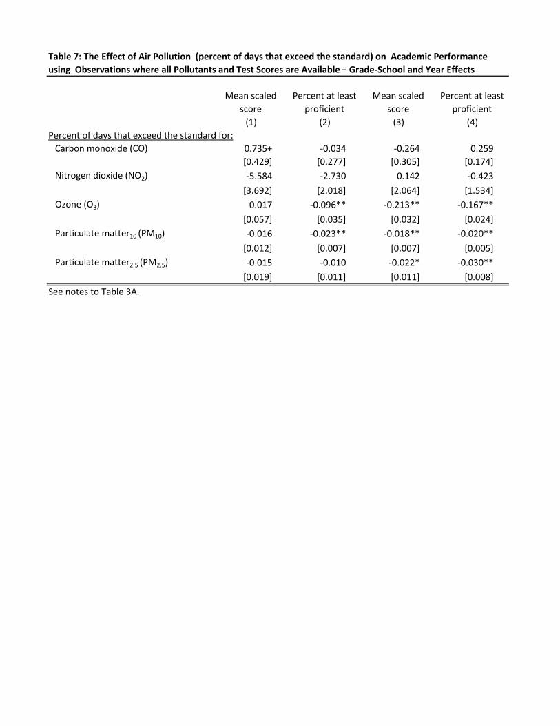
Mean scaled 

score

Percent at least 

proficient

Mean scaled 

score

Percent at least 

proficient

(1) (2) (3) (4)

Percent of days that exceed the standard for:

Carbon monoxide (CO) 0.735+ ‐0.034 ‐0.264 0.259

[0.429] [0.277] [0.305] [0.174]

Nitrogen dioxide (NO2) ‐5.584 ‐2.730 0.142 ‐0.423

[3.692] [2.018] [2.064] [1.534]

Ozone (O3) 0.017 ‐0.096** ‐0.213** ‐0.167**

[0.057] [0.035] [0.032] [0.024]

Particulate matter10 (PM10) ‐0.016 ‐0.023** ‐0.018** ‐0.020**

[0.012] [0.007] [0.007] [0.005]

Particulate matter2.5 (PM2.5) ‐0.015 ‐0.010 ‐0.022* ‐0.030**

[0.019] [0.011] [0.011] [0.008]

Table 7: The Effect of Air Pollution  (percent of days that exceed the standard) on  Academic Performance 

using  Observations where all Pollutants and Test Scores are Available − Grade‐School and Year Effects 

See notes to Table 3A.

Quantile 10% 20% 40% 50% 60% 80% 90%

(1) (2) (3) (4) (5) (6) (7)

Carbon monoxide (CO) 0.496 0.087 0.022 0.52 0.266 0.412 0.536

[0.478] [0.498] [0.555] [0.411] [0.401] [0.766] [0.438]

Nitrogen dioxide (NO2) ‐5.615 ‐3.786 ‐7.393** ‐5.151* ‐4.437* ‐3.245 ‐5.056*

[4.288] [3.228] [2.778] [2.327] [2.101] [2.374] [2.579]

Ozone (O3) 0.005 0.012 0.019 0.016 0.005 ‐0.034 ‐0.051+

[0.030] [0.024] [0.021] [0.018] [0.020] [0.024] [0.028]

Particulate matter10 (PM10) ‐0.024** ‐0.027** ‐0.022** ‐0.017** ‐0.022** ‐0.025** ‐0.020**

[0.0056] [0.0044] [0.0043] [0.0038] [0.0039] [0.0050] [0.0060]

Particulate matter2.5 (PM2.5) 0.0007 ‐0.021* ‐0.025** ‐0.030** ‐0.029** ‐0.046** ‐0.048**

[0.012] [0.0010] [0.0090] [0.010] [0.012] [0.0086] [0.012]

Carbon monoxide (CO) ‐0.641 ‐0.340 ‐0.256 ‐0.338+ ‐0.364+ ‐0.274 ‐0.332

[0.409] [0.414] [0.388] [0.200] [0.199] [0.378] [0.457]

Nitrogen dioxide (NO2) ‐3.042 ‐1.878 ‐3.340** ‐4.066** ‐4.685** ‐4.462** ‐4.347+

[2.228] [1.759] [1.229] [1.395] [1.257] [1.729] [2.308]

Ozone (O3) ‐0.040* ‐0.066** ‐0.095** ‐0.105** ‐0.116** ‐0.143** ‐0.151**

[0.016] [0.014] [0.013] [0.014] [0.013] [0.016] [0.021]

Particulate matter10 (PM10) ‐0.017** ‐0.020** ‐0.025** ‐0.026** ‐0.030** ‐0.030** ‐0.032**

[0.0040] [0.0029] [0.0030] [0.0031] [0.0033] [0.0038] [0.0047]

Particulate matter2.5 (PM2.5) 0.012 0.0054 ‐0.0063 ‐0.011* ‐0.022** ‐0.028** ‐0.032**

[0.0077] [0.0060] [0.0051] [0.0050] [0.0055] [0.0063] [0.0066]

Carbon monoxide (CO) ‐0.998* ‐0.744* ‐0.502+ ‐0.339 ‐0.540** ‐0.574+ ‐0.609*

[0.469] [0.332] [0.264] [0.235] [0.185] [0.348] [0.290]

Nitrogen dioxide (NO2) 0.422 ‐1.072 ‐1.777 ‐0.967 ‐0.501 ‐0.639 0.258

[2.658] [1.494] [1.440] [1.676] [1.137] [1.703] [2.914]

Ozone (O3) ‐0.191** ‐0.205** ‐0.196** ‐0.211** ‐0.222** ‐0.224** ‐0.262**

[0.015] [0.012] [0.012] [0.012] [0.013] [0.012] [0.020]

Particulate matter10 (PM10) ‐0.014** ‐0.015** ‐0.019** ‐0.021** ‐0.021** ‐0.022** ‐0.025**

[0.0047] [0.0038] [0.0026] [0.0026] [0.0023] [0.0030] [0.0039]

Particulate matter2.5 (PM2.5) ‐0.022** ‐0.026** ‐0.028** ‐0.029** ‐0.029** ‐0.024** ‐0.027**

[0.0063] [0.0051] [0.0047] [0.0044] [0.0047] [0.0064] [0.0069]

Carbon monoxide (CO) 0.320+ 0.168 0.153 0.074 ‐0.032 ‐0.021 ‐0.186

[0.194] [0.140] [0.230] [0.171] [0.107] [0.214] [0.247]

Nitrogen dioxide (NO2) ‐2.148 ‐1.826 ‐2.069+ ‐1.164 ‐0.576 ‐0.258 0.687

[1.448] [1.368] [1.164] [1.220] [1.482] [1.523] [1.266]

Ozone (O3) ‐0.142** ‐0.149** ‐0.163** ‐0.178** ‐0.182** ‐0.204** ‐0.252**

[0.013] [0.010] [0.008] [0.010] [0.011] [0.013] [0.016]

Particulate matter10 (PM10) ‐0.019** ‐0.017** ‐0.019** ‐0.020** ‐0.020** ‐0.022** ‐0.023**

[0.0027] [0.0022] [0.0022] [0.0025] [0.0023] [0.0027] [0.0035]

Particulate matter2.5 (PM2.5) ‐0.024** ‐0.023** ‐0.029** ‐0.036** ‐0.036** ‐0.033** ‐0.036**

[0.0050] [0.0046] [0.0033] [0.0032] [0.0032] [0.0047] [0.0060]

Table 8: Quantile Regressions Results for Mathematics and English/Language Arts

See notes to Table 3a.

Panel A:  Mathematics Mean Scaled Score

Panel B: Percent at Least Proficient in Mathematics

Panel C: English/Language Arts Mean Scaled Score

Panel D: Percent at Least Proficient in English/Language Arts

Quantile 10% 20% 40% 50% 60% 80% 90%

 Mathematics 

 Mean scaled score  310.2 324 344.5 354 364.3 389.9 410.2

 Percent at least proficient  22 31 44 50 57 71 80

 English/language arts 

 Mean scaled score  306 316.3 331.7 339.1 346.7 365.9 380.3 Percent at least proficient  17 24 35 41 48 63 74

Table 9: Distribution of Outcome Variables