political economy of corporate tax avoidance V2

The Political Economy of Corporate Tax Avoidance

Qiao Liu

GuanghuaSchool of Management

PekingUniversity

Beijing 100871, China

Phone: 86-10-6276-7993

Email: [email protected]

Wei Luo*

GuanghuaSchool of Management

PekingUniversity

Beijing 100871, China

Phone: 86-10-6275-0961


Pingui Rao

Jinan University

Guangzhou 510632, China

Phone: 86-20-8522-5976


March 15, 2015

2

The Political Economy of Corporate Tax Avoidance

Abstract: This paper employs a new empirical approach for identifying the impact of

politicians’ opportunistic policy preferences on corporate tax avoidance. Our key innovation

is to use turnovers of local politicians as a source of exogenous variation in tax enforcement

efforts, which have strong implications for firms’ strategic tax avoidance decisions. Using

data on turnovers of China’s municipal political leaders and industrial firms in their

jurisdictions, we document cycles in corporate tax avoidance corresponding with the timing

of local politician turnovers. The political cycle of tax avoidance is more pronounced in

municipal cities with strong tax base and weaker governance. The cycle occurs when a local

politician is younger and follows an upward career trajectory. The tax avoidance cycle is also

more evident among firms that can potentially derive higher value from strategically engaging

in tax avoidance activity. Our findings suggest that varying tax enforcement driven by local

politicians’ policy preferences is an important channel – entirely different from the political

uncertainty and political connection channels – through which the political process affects

real economic activity.

Keywords: political turnovers; tax avoidance cycle; enforcement; political economy.

JEL Code: G31; G34; H26; K42; P48

3

1. Introduction

Tax avoidance is a strategic corporate practice pervasive in both developed and emerging

markets (e.g., Slemrod, 2004; Desai and Dharmapala, 2006; and Cai and Liu, 2009). Firms

strategically trade off the benefits and potential costs of engaging in tax avoidance activity.

This tradeoff however could be significantly influenced by politics, since politicians’

opportunistic policy choices have strong implications for their tax enforcement efforts. In

facing opportunistic tax enforcement efforts, firms strategically engage in tax avoidance

activity to maximize their interest. This political economic perspective of tax avoidance

however has not been investigated in the literature. 1

In this paper, we employ a new

empirical approach to identify the impact of politicians’ opportunistic policy preferences on

corporate tax avoidance. Specifically, we use turnovers of China’s municipal political leaders

as a source of exogenous variation in tax enforcement efforts, and study how varying tax

enforcement efforts affect firms’ strategic tax avoidance decisions.

The motivation of our empirical study is two-fold. First, the literature on political

business cycle proposes that the incumbent politicians strategically use fiscal and monetary

policy instruments to maximize the probability of being re-elected (e.g., Nordhaus, 1975;

Rogoff and Sibert, 1988; and Rogoff 1990). Empirical studies show that government spending

and macroeconomic outcomes such as inflation and unemployment display cyclical patterns

following the cycles of political events such as elections or government turnovers.2 We

extend this argument to tax enforcement and corporate tax avoidance by documenting a

similar tax avoidance cycle corresponding to the timing of political turnovers.

Second, investigating the impact of tax enforcement efforts on corporate tax avoidance

activity is unavoidably plagued by two sources of endogeneity concern: (i) excessive tax

avoidance activities may trigger more enforcement efforts; and (ii) both tax avoidance and tax

enforcement efforts could be affected by unobserved common factors (i.e., adverse business

1 Desai, Dyck, and Zingales (2007) is a notable exception. They study an episode of increased tax

enforcement in Russia following the election of Vladimir Putin. 2 For example, see Levitt, 1997; Akhmedov and Zhuravskaya, 2004; Brender and Drazen; 2008; and Liu

and Ngo, 2014.

4

conditions). Turnovers of local politicians provide an interesting setting to resolve these two

sources of endogeneity. Politicians face limited terms and may be replaced by others with

different policy preferences. While tax laws remain relatively stable, the extent to which they

are enforced depends on politicians’ policy preferences. Political turnovers lead to shifting

policy preferences, which generate plausible exogenous variation in tax enforcement efforts,

and allow us to disentangle the endogeneity between tax avoidance and tax enforcement.

We use data on turnovers of China’s municipal political leaders and industrial firms in

these leaders’ jurisdictions to examine how incentives and policy preferences faced by local

politicians affect strategic corporate tax avoidance decisions. During China’s reform era, local

politicians have significant autonomy in economic matters. Municipal political leaders are

assessed and promoted primarily based on local economic growth. Political tournaments

based on economic growth push local officials to focus on measureable objectives such as

GDP growth (Maskin et al., 2000; Li and Zhou, 2005; and Xu, 2011). Local politicians,

during the early period of their terms, have stronger incentives to perform well in the between

region economic competition. Strengthening tax enforcement to exploiting local tax base

more effectively is a convenient choice. Enhancing enforcement efforts not only generates

immediate effects on fiscal revenue but also enhances local governments’ borrowing capacity.

In addition, tax enforcement and tax policy adjustment give local politicians more latitude to

engage in rent-seeking activity (Shleifer and Vishny, 1993).

However, strengthened tax enforcement can hardly last long. Unfavorable changes in tax

enforcement may drive out investments and business activities.3 In the regional economic

competition, tax enforcement may become a bargaining tool to attract new businesses. Lax

tax treatment demonstrates local government’s commitment to new projects. As different

regions compete on economic growth driven by new businesses and new investments,

tightened enforcement may in the long run hurt local politicians’ interest. Local politicians

thus may choose to loosen up tax enforcement gradually. Reacting to local politicians’

3 Existing business may move new projects to regions that provide beneficial tax treatments, or shift

their income through transfer pricing to other regions (Shevlin et al., 2012).

5

shifting tax enforcement efforts, firms conduct tax avoidance activity accordingly. We thus

expect a tax avoidance cycle of corresponding to the timing of local political turnovers.4

Using a hand-collected dataset of local political leaders in more than 300 municipal

cities in China during 1999-2007, we examine how political turnovers affect corporate tax

avoidance. A local politician typically follows a five-year term in China. However, most

could not complete their terms (Landry et al., 2014).5 Turnovers of local politicians are

largely unexpected and out of the control of any individual firm. We therefore exploit this

exogenous timing of political turnovers to mitigate the potential endogeneity. Meanwhile, as

Chinese local politicians have no legislation discretion in making their own tax laws, our

results are exempted from the effects of tax law modifications by local politicians.

Furthermore, turnovers of municipal political leaders take place at different points in time,

allowing us to net out market-wide trends in corporate tax avoidance.

Consistent with our proposed political economic hypothesis, we find a cyclical pattern of

corporate tax avoidance. Specifically, we find novel and robust evidence that firms exhibit

weaker incentives to conduct tax avoidance activity in the first year of a municipal political

leader’s term. They however increase the extent of tax avoidance over time until the local

politician is replaced by a new one.

As a further analysis, we exploit a natural experiment which generates exogenous

variation in local politicians’ tax enforcement efforts – the 2002 tax regulation change that

significantly reduced politicians’ capabilities to time tax enforcement efforts (see Section 2.2

for details). We find robust evidence that that after 2002, the political cycle of corporate tax

avoidance becomes less evident. We also find that when the 2002 regulation change

occurred during a politician’s early (late) period of his term, firms in his jurisdiction exhibit

weak (strong) incentives to avoid tax. These findings are consistent with our political

economy hypothesis.

4 In a similar spirit, Huang (1996) documents a cycle of investment corresponding to the timing of

political turnovers in China. Huang (1996) proposes that politicians’ career concern push them to

encourage more investment during the earlier period of their terms. 5 In our sample, for the period from 1999 to 2007, the average tenure of municipal political leaders

(i.e., party secretaries) is 2.95 years, while the median tenure is 1.8 years, as shown in Table 2.

6

To address the possibility that turnovers of municipal political leaders may be correlated

with omitted variables which have implications for firms’ tax avoidance activity. We analyze

a refined subsample in which turnovers of local politicians are due to sudden deaths,

“Shuanggui” (under investigation), or dismissal from office.6 We conduct a

difference-in-differences (DID) analysis and find that after the sudden change of a local

political leader, firms operating in his jurisdiction engage less in tax avoidance. The economic

effect of sudden political turnovers on tax avoidance is sizable. We find that after the sudden

turnover of a local politician, firms reduce their tax avoidance level by as much as 12.3%.

While we provide robust evidence that the politics process, through the time-varying tax

enforcement efforts, impact on corporate tax avoidance, we have to rule out alternative

political channels.7 Political uncertainties brought about by political turnovers may lead to a

similar tax avoidance cycle too. When a new municipal political leader takes his position,

firms in his jurisdiction may not know much about his policy preferences and management

style. These firms hence may behave more cautiously and reduce tax avoidance. Over time, as

the new leader gradually reveals his policy preferences, firms engage more in tax avoidance.

If the political uncertainty hypothesis holds, we expect the tax avoidance cycle to be less

pronounced in municipal cities whose new leaders were promoted from within. However, we

document a more pronounced cycle in cities whose new leaders come from inside. This

evidence does not support the political uncertainty hypothesis.

Another prominent competing explanation is the political connection hypothesis.

Politically connected firms may enjoy a wide range of benefits including preferential access

to external financing, government contracts, tax benefits, government subsidies, and favorable

policies. However, around political turnovers, established political connections are most likely

6 “Shuanggui” is a special scheme implemented by the discipline unit of China ruling party (CCP). This

practice literally means that the involved party members have to confess his wrongdoings in the

specified place and during the specified time period. When “Shuanggui” happens on a certain party

member, he will be placed under custody. Removal from office normally applies to officials who have

committed crimes and it is a harsher penalty than “shuanggui”. 7 A large and growing literature examines the effects of political or policy uncertainties on real

decisions and economic outcomes. For example, Bernanke (1983), Bloom, Bond, and Van Reenen

(2007), and Julio and Yook (2012) study the relationship between political uncertainties and real

investment.

7

broken and it takes time to foster strong connections to the new leaders. Reducing tax

avoidance is therefore a firm’s natural response to lost political connections. In addition, it

helps appease new leaders’ desire to secure more resources. This political connection

hypothesis may explain the political cycle of tax avoidance as well. However, our evidence

does not support this hypothesis. In particular, when a new leader is promoted from within,

firms’ political connections to him still remain, we expect firms to engage in more tax

avoidance during early periods of new leader’s term. We find exactly the opposite.

If our political economy hypothesis holds, we should expect the magnitude of the

political cycle of tax avoidance to vary with region, politician, and firm level characteristics.

It should be more evident in regions where the politicians have stronger incentives and

capabilities to time enforcement efforts. It should also be more evidence among firms that can

potentially derive higher value from strategically engaging in tax avoidance activity, in

response to local governments’ time varying enforcement efforts.

We find robust evidence. Across regions, we find that the political cycle of tax avoidance

is more pronounced in municipal cities with deeper tax base (measured by local fiscal revenue

over local GDP) and poorer public governance (measured by the value of marketization level

scored by a given city). In both cases, the local politicians can benefit more from tightening

up tax enforcements.

On a related point, we find that the age of municipal politicians and their career

trajectories significantly matter. Young politicians (under 45 years old) usually have more

time to climb the political hierarchy and thus, have stronger incentives to participate in the

political tournament. When they approach the required retirement age (60 years old), they are

less incentivized to time their efforts. Similarly, when a politician follows an upward career

trajectory (i.e., he was promoted from a lower rank to the current post), he may demonstrate

stronger incentives to perform as well. We find that the political cycle of corporate tax

avoidance is more evidence in regions where the local politicians are young, and follow an

upward career trajectory.

Within regions, we find that the effects of political turnovers on tax avoidance vary

8

across several firm characteristics. Specifically, we document that the political cycle of tax

avoidance is more pronounced for non state-owned firms, small firms, and less fiscally

important firms. Furthermore, we find evidence that the tax avoidance cycle is more

pronounced for less efficient firms measured by lower total factor productivity (TFP) and

higher administrative expenses.

The findings in this paper have three important contributions. First, we document a new

stylized fact regarding corporate tax avoidance, namely, a political cycle of corporate tax

avoidance. This result demonstrates an important link between the political process and real

economic activity. Our paper is thus related to a growing literature that documents the

economic consequence of politics. Specifically, Julio and Yook (2012) investigates how

political turnovers impact on corporate investment through the political uncertainty channel.

The literature has also documented the effects of political turnovers on initial public offering

(Colak et al., 2013), industry return volatility (Boutchkova et al., 2012), and cash flows and

stock returns (Kim et al., 2012; and Belo et al., 2013).

Second, we provide evidence suggesting that tax enforcement efforts are associated with

politicians’ changing policy preferences, and hence time-varying. We thus contribute to the

literature on the relation between tax enforcement and tax avoidance.8 A major obstacle

limiting empirical progress in this literature is the difficulty in identifying changes to tax

enforcement efforts as truly exogenous. Tax enforcement efforts are influenced by firm

behavior and developments in corporate sector. Using turnovers of municipal political leaders

as a source of exogenous variation in tax enforcement efforts allow us to overcome this

challenge and shed considerable light on the impact of tax enforcement on tax avoidance

activity.

Third, our study adds to a large literature identifying the determinants of corporate tax

8 Not many studies directly test for the effect of tax enforcement on tax avoidance. Hoopes et al.

(2012) find that U.S. public firms undertake less aggressive tax positions when tax enforcement is

stricter (IRS monitoring). Gupta and Lynch (2012) examine the tax enforcement at state level and find

that enhanced corporate tax enforcement results in the increase in state tax collections two years into

the future. They also find that enforcement and restrictive tax policies are substitutes. DeBacker et al.

(2013) find that corporations increase their tax aggressiveness after an audit for a few years and then

reduce it gradually.

9

avoidance including corporate governance (e.g., Desai and Dharmapala, 2006; and McGuire,

Wang, and Wilson, 2014), industry competition (Cai and Liu, 2009), financial constrains

(Edwards et al., 2014), and credit information sharing systems and higher branch penetration

(Beck et al., 2014). We find that politicians’ policy preferences determine their tax

enforcement efforts, which lead to a political cycle of corporate tax avoidance. On this

particular point, our paper is related to Scholz and Wood (1998), Young et al. (2001), and

Bagchi (2013).9

The rest of this paper proceeds as follows. Section 2 provides institutional background

and testable hypotheses. Then Section 3 discusses data and empirical strategy, and research

design. Section 4 presents our empirical findings. Section 5 provides cross-sectional evidence.

Section 6 concludes.

2. Institutional Background and Hypotheses Development 2.1. Career paths and policy preferences of local politicians in China

The development in China during its reform era can be characterized by political

centralization and economic decentralization (Xu, 2011). Political centralization means that

the ruling party (CCP) has complete control over officials at all levels within the political

system. The party’s cadre management system is responsible for cadre appointment and

promotion decisions in both the CCP and governments at all levels. To achieve an effective

control, CCP builds up branches matching different levels of the government system. At the

regional level, party secretary is the highest ranked political leader and has political power

higher than the highest ranked government official at the same level.

Through its organization departments at different levels, CCP applies “one-level down”

appointment system (Huang 1996; Landry 2008). The evaluation of local officials lies in the

hands of party officials at a higher level. CCP frequently rotates the party officials to cope

9 Scholz and Wood (1998) find that IRS audits for corporate and individual increase with increased

Democratic control over Congress and change with different presidential administrations. Young et al.

(2001) find that the IRS audit rate of individual income tax is significantly lower in districts that are

important to the president electorally and that have representation on key congressional committees.

Bagchi (2013) shows the influence of political ideology on the enforcement of the nation’s tax laws.

Under Democratic administrations, budget devoted to detecting tax fraud and audit probabilities for

corporations are significantly higher.

10

with local officials’ entrenched interests and fight against corruption. Notably, formal

personnel regulations imposed by CCP put strict rule on the retirement age: 60 years old for

all officials below the rank of governor or provincial party secretary and 55 years old for

female officials.

Typically, a municipal political leader (i.e., party secretary at the municipal city level)

has several career paths. He may be purged due to misbehavior such as corruption; he may be

relegated to an honorary post (i.e., head of political advisory commission) within the same

city; he may be transferred to other region, a functional department of the party or the

government, non-governmental organizations, and state enterprises. At the municipal city

level, a mayor typically serves concurrently as (first) deputy secretary of the municipal CCP

committee. Taking the post of municipal party secretary suggests a promotion. Of course, he

may be promoted to a more senior position at the provincial level, and in some unusual cases,

to a position at the central government level.

To advance political career, a local official needs to demonstrate his competence and

political loyalty (Nathan and Gilley 2002). During China’s reform era, China’s local

governments have significant autonomy in economic matters (Xu, 2011). Regional

decentralization empowers local officials over economic development, public services and

law enforcement within their jurisdictions. They enjoy the flexibility in enforcing laws,

levying taxes, providing subsidies, and regulating competition. In addition, they directly

control state-owned enterprises (SOEs) at their region. They can select the SOE managers,

and significantly influence SOEs’ investment and operating decisions. Local officials who can

signal better outcomes of their autonomous power against their peers are likely to benefit by

gaining access to the next level of political power.

Given such an institutional arrangement, local leaders compete for performance-based

political promotion and GDP growth is a key performance indicator (Li and Zhou, 2005).

Shih et al. (2012) identify factional ties with various top leaders, educational qualifications,

and provincial revenue collection as key factors in explaining promotion outcomes of

provincial leaders. Landry (2008) extends the analysis to the prefectural level of cities, and

11

finds that economic progress measured as GDP per capita over its value at the beginning of

the appointment is positively related to promotion (locally and/or externally) of city mayors.

Landry et al. (2014) further show that growth in fiscal revenue play a critical role in the

promotion decisions of local officials at provincial, municipal, and county-level.

2.2. Income tax systems in China and tax enforcement

As Acemoglu and Robinson (2006) suggest, authoritarian leaders prioritize tax collection

capacity. Facing powerful incentives to perform, taxes are convenient and effective tools for

local officials to obtain resources for local development.

A series of tax reforms since 1994 result in fiscal decentralization of China. Under this

system, the central government and the local governments have their own tax territories and

their own tax bureaus-the state tax bureaus and the local tax bureaus respectively. The

legislation power of tax rests on the center. But the local governments can issue rules or

policies to facilitate the implementation of the tax laws, regulations and rulings of the central

government. In order to compete for local economic growth, many local governments even

provide various tax incentives without proper authorization from the center. For instance, Wu

and Yue (2009) illustrated tax rebate policy by the local governments under which listed firms

first paid income tax at the nominal tax rate of 33% and then the local governments refunded

them 18% in order to attract businesses.

The central government and the local governments share responsibility to collect

enterprise income tax. From 1994 to 2001, the state tax bureaus collected income tax on SOEs

directly controlled by the central government and all the foreign enterprises. The local tax

bureaus were responsible for income tax of local SOEs, collective firms, and private firms.

During this period, the sharing ratio between the central and the local governments was 40%

vs. 60%. On December 31, 2001, the State Council issued a circular to adjust the taxation

scope of the state and the local tax bureaus and change the sharing ratio of enterprise income

tax.10

Beginning 2002, all new companies paid income taxes to the local branches of the state

10

the Circular of the State Council on Distributing the Scheme on the Reform of Income Tax Revenue Sharing

(GuoFa [2001] No.37).

12

tax bureau. But the local governments continued to levy income taxes from the existing local

firms registered prior to 2002. In 2002, the central government and the local governments

shared the income tax equally. The sharing ratio has settled at 60% vs. 40% beginning 2003.

The 2002 regulation change reduced the local governments’ capabilities to levy income tax. A

further adjustment occurred in 2008. Since 2009, all new domestic firms which pay

value-added tax (VAT) should pay income tax at the state tax bureaus, while the firms paying

business tax should pay at the local tax bureaus. The restructuring of collection scope presents

an exogenous shock to the local governments’ tax responsibilities.

Local governments can affect tax enforcement through the structure of the local tax

bureau system since the management of the local tax bureaus is subject to the organic law of

the local governments. The local tax bureaus at provincial level are under the dual leadership

of the provincial government and the State Administration of Taxation (SAT) at the central

government level. The local tax bureaus below the provincial level are accountable to both the

tax authorities at higher level and the governments at the same level. The dual leadership

model enables local government to exert influence on tax enforcement of the local tax bureaus.

Anecdotal evidence confirms the influence of local politicians on tax enforcement. For

instance, when the central committee of the communist party of china removed Xilai Bo from

his duty on March 15, 2012, the executive vice-mayor of Chongqing emphasized the first task

for the Bureau of Finance was to enhance tax enforcement.11

Tightened tax enforcement could be a double-edged sword. On the one hand, tightened

tax enforcement brings in more fiscal revenue and quickly improves fiscal condition. On the

other hand, it may push existing business to other regions. It may also drive out new

investments and new projects. The negative consequences of tax enforcement efforts put local

officials in a disadvantage position of regional competitions (Maskin et al., 2000). Local

officials strategically choose tax enforcement efforts to strike a careful balance between the

benefits and costs of tightening up tax enforcement.

2.3 Testable hypotheses

11

Source: 21st Century Business Herald, February 1, 2013.

13

Political tournaments based on economic growth simply push local politicians to focus

on measureable objectives such as GDP growth driven by investments, especially public

sector investments. Huang (1996) documents a political cycle of real investments by showing

that a region tends to make more fixed asset investments during the early period of the local

politician’s term. To make more investments, the local politicians, during the early period of

their terms, have stronger incentives to secure enough resources for investments and economy

growth. Increasing tax enforcement efforts is a natural choice. In responding to such an

exogenous shock in tax enforcement, firms may strategically adjust down their extent of tax

avoidance. We thus expect:

Hypothesis 1: all else equal, firms’ incentives to engage in tax avoidance are weak

during the early period of the municipal political leaders’ terms. Especially, the level of tax

avoidance is the lowest in the first year of new leaders’ terms, and increases over time within

their terms.

As we conjecture that a possible political cycle of tax avoidance is driven by local

politicians’ time-varying tax enforcement efforts resulting from their policy preferences, we

expect cross-region variation in corporate tax avoidance. We have

Hypothesis 2: all else equal, the political cycle of tax avoidance tends to be more evident

in regions with strong fiscal capacity and poorer public governance.

We also expect the political cycle of corporate tax avoidance to be related to local

politicians’ personal attribute and career concerns. We expect young politicians and politicians

promoted from lower ranks to demonstrate stronger incentives to excel in the political

tournament for economic growth. We have

Hypothesis 3: all else equal, the political cycle of corporate tax avoidance tends to be

more evident in regions whose local leaders are younger and are promoted from lower ranks.

Moreover, since firms strategically conduct corporate tax avoidance activities to appease

local politicians’ desires for economic growth, we expect the political cycle of tax avoidance

to be related to several firm specific characteristics. We conjecture that firms have stronger

incentives to strategically engage in tax avoidance activity when they are small-sized, private,

14

less important to improving local fiscal conditions, less advanced in technology, and poorly

governed. We thus have

Hypothesis 4: all else equal, the political cycle of corporate tax avoidance tends to be

more evidence for smaller firms, private firms, firms that are less critical to improving local

fiscal conditions, less technologically advanced firms, and finally, firms that are poorly

governed.

3. Data and Empirical Design

3.1. Sample

Our initial sample consists of all firm-year observations between 1999 and 2007 in the

Chinese Industrial Enterprises Database (CIED) developed and maintained by the National

Bureau of Statistics of China (NBS). This database consists of all industrial firms with sales

over five million RMB.12

Our sample ends in 2007 to avoid the effects of the 2008 tax reform

in China and the global financial crisis.

For all municipal cities in China, we manually collect information on terms and personal

backgrounds of the local political leaders including CCP party secretaries at the city level (our

primary focus) and mayors. In the context of the Chinese politics, a party secretary usually is

the top political leader in that region. A mayor typically also takes the post of deputy party

secretary, and is usually No.2 political figure in a certain municipal city. The information

sources are local government websites, news releases, the Renminwang website

(www.people.com.cn), and other public announcements. We also collect resumes of district

heads for four province-equivalent municipal cities (Beijing, Tianjin, Shanghai, and

Chongqing), because these officials have the same political rank as party secretaries at a

municipal city level. The fiscal information and GDP information come from the National

Municipal City Prefecture, and County Finance Statistics Compendium (Quanguo Di Shi

Xian Caizheng Tongji Ziliao), published by the Ministry of Finance annually.

Combining the aforementioned data sources, we impose the following criteria to reach

the final sample: (1) there is no missing information on critical parameters including firm

12

See Cai and Liu (2009) for a detailed description of NBS’ CIED database.

15

headquarter location, total assets, sales, the number of employees, gross value of industrial

output, net value of fixed assets, firm ownership type and tax payable; (2) total assets and/or

sales are greater than 1 million RMB and the number of employees is greater than 30; (3)

current assets, non-current assets, total fixed assets, depreciation expense, tax payable and

Industrial value added per capita are greater than zero; (4) accumulated depreciation is greater

than annual depreciation expense, and tax payable is less than pre-tax profit; (5) net income

deflated by total assets is within three standard deviations; (6) city-level information on GDP

and fiscal revenue is not missing.

From this procedure, we obtain 1,337,323 firm-year observations and 3227 municipal

city-year observations. Panel A of Table 1 describes sample distribution over years. The final

sample covers 31 provinces, and 406 municipal cities or municipal city equivalent

administrative units. Due to coding errors of firm headquarters in CIED, firms from

Chongqing cannot be identified during 1999-2003. The turnover rate of municipal political

leaders indicates the percentage of cities experiencing a turnover of party secretary. In a given

year, close to 25% of cities experience turnovers of political leaders.

3.2. Terms of Municipal City Political Leaders

We focus our analysis on party secretaries at the municipal city level. For each local

leader, we identify the date of his taking office. If the date is before July 1, then the year is

counted as the first year of this politician’s term. If the date is after July 1, then the first year

of the politician’s term is specified as the following year. We construct a dummy variable,

First, which takes the value of 1 if a certain year is the first year of the local politician’s term

and 0 otherwise. For each local leader, we also define a variable labeled Tenure, which equals

1 for the first year of the leader’s term, and accumulates on a yearly basis within the same

leader’s term.

Panel B of Table 1 shows that majority (70%) of 1101 local political leaders in our

sample failed to complete a five-year term. Only 14% served a complete first term, and 15%

of local politicians started a second term. The longest service was 11 years. Consistent with

Landry et al. (2014), these results indicate a political process unique to the Chinese political

16

context.

(Place Table 1 Here)

3.3. Measures of Corporate Tax Avoidance

The extent of corporate tax avoidance cannot be directly observed. Following Cai and

Liu (2009), we measure the level of tax avoidance by the sensitivity of reported profits to

imputed profits based on the national income accounting. The imputed profits are obtained

based on the following equation:

, , , , , , ,Imputed Profit (1)i t i t i t i t i t i t i tOutput Inputs Depreciation FC Wage VAT= + − − − −

where Output is a firm’s gross value of industrial output; Inputs measures its intermediate

inputs excluding financial charges; Depreciation is the annual depreciation expense; FC is

financial charges including interest payments; Wage is wages and salaries; VAT is

value-added tax paid. We define PRO as the imputed profit in Equation (1) deflated by total

assets. A firm’s pre-tax profit is defined as the reported profit. We define RPRO as pre-tax

profit deflated by total assets.13

3.4. Empirical Specifications

To test for the political cycle of corporate tax avoidance, we primarily run the following

regression model:

, 0 1 2 3 4 5 6 7

8 9 , 1

2 3 4 5 6

( +

)

+

i t

i i i t

i year i location

RPRO Tenure Tax Finance Labor Rsales SOE PCHG

Mtenure GDPG Year Location PRO Tenure

Tax Finance Labor Rsales

β β β β β β β β

β β β β α

α α α α α

= =

= + + + + + +

+ + + + +

+ + + +

∑ ∑

7 8

9 (2)i i

i year i location

SOE PCHG Mtenure

GDPG Year Location

α α

α α α= =

+ +

+ + +∑ ∑

In the model, we use two variables to measure the tenure of local politician, First and Tenure.

We expect local political leaders to tighten up tax enforcement during the early period of their

terms. First should have a positive sign (that is, β1 > 0), indicating lower tax avoidance. If

13

As explained in Cai and Liu (2009), the gap between RPRO and PRO comes from exogenous

differences in the generally accepted accounting standards and the national income account system.

The two systems have different rules on depreciation, revenue and expenses recognition. Although

PRO and RPRO are legitimately different, Cai and Liu (2009) show that under certain conditions, the

sensitivity of RPRO to PRO is a good proxy for the extent of tax avoidance.

17

there is a political cycle of tax avoidance, Tenure should have negative a sign (that is, β1 < 0),

suggesting that level of corporate tax avoidance increases with the local politicians’ tenure.

We include a battery of control variables. We define effective tax rate, TAX, as income

tax payable over reported pre-tax profit. The measure is set to zero for loss-making firms. In

our analysis, we exclude observations with TAX greater than one. When a firm is more

financially constrained, it may have stronger incentives to engage in tax avoidance activity

(Edwards et al. 2014). As suggested in Allen et al. (2005), access to bank loans reflects a

firm’s ability to borrow. We compute the ratio of financial expenses to total assets (Finance),

and use it as a proxy for external financing constraint. Higher financial expenses may indicate

more borrowing, and thus less tight financing constraint, which consequently may reduce the

firm’s incentive to engage in tax avoidance activity.

We control for firm size, which is measured as the logarithm of the number of

employees (Labor). While large firms have more resources to conduct tax avoidance activity

(e.g. Mills et al. 1998), they tend to draw more attentions and hence may face a higher risk of

being detected. How firm size affects corporate tax avoidance is thus an empirical issue. To

account for the impact of the differences in the accounting standards and the national income

account system, we create a variable, Rsales, which is the ratio of sales to industrial output.

Dummy variable, SOE, takes the value of 1 if a firm is state owned and 0 otherwise.

Bradshaw et al. (2013) suggest that managers of SOEs have strong incentives to pay income

tax due to career concerns.

We construct three variables to account for municipal city-level characteristics. GDPG,

the percentage change of GDP of the city, captures the economic condition of a certain city.

Poterba (1994) finds that economic downturns and election years significantly affect state

taxes and spending. When the economy is growing, the politicians have weaker incentives to

tighten tax enforcement. PCHG, a dummy variable taking the value of 1 if there is a turnover

of governor or provincial party secretary, captures the political uncertainty surrounding a

certain municipal city. Facing political uncertainty, a firm may avoid more tax. We also

control the tenure of mayor, the No.2 political figure in a municipal city. Moreover, we create

18

geographical dummies at province level and year dummies.

3.5. Descriptive Statistics

We present summary statistics of key variables in Table 2. All continuous variables are

winsorized at 1% and 99%. Panel A of Table 2 reports the statistics of city-level variables.

Notably, majority of local political leaders are male (97.9%). The average age of municipal

city party secretaries is 51 year old. The mean value of First is 0.246, suggesting that 24.6%

of local political leaders in our sample are in the first year of their terms. The average local

leaders’ tenure duration (Tenure) is 2.945 years, longer than that of mayors (Mtenure), which

is 2.672 years. Local is a dummy variable that takes the value of 1 if the local political

leader’s previous job was in the same city and 0 otherwise. We find that 45% of party

secretaries at the municipal city level are local. As a dummy variable, Promoted takes the

value of 1 if a political leader’s current rank is higher than that of his previous job, and 0

otherwise. In our sample, 17.8% of local politician are promoted from a lower rank to the

current position.14

Variation in local economic, political, and fiscal conditions is quite substantial. 23% of

municipal cities locate in provinces where either governor or provincial party secretary has

been replaced. Average GDP growth rate at the municipal city level is 14.7% during our

sample period. FiscalR, defined as the ratio of total fiscal revenue to GDP, has a mean value

of 0.142 and a median value of 0.112. GCTAX_GDP, which measures the growth rate of

fiscal revenue minus the GDP growth rate, has a mean value of 0.226, suggesting that fiscal

revenue grows faster than GDP during our sample period.

Panel B of Table 2 presents the summary statistics of firm level variables. The reported

profit (RPRO) has a mean of 0.073, far smaller than that of the imputed profit (PRO), which

stands at 0.248. We construct a variable GAP to capture the extent to which the two profit

measures differ. GAP, defined as RPRO minus PRO and then deflated by PRO, has a mean

14

Under the Chinese political system, mayors and party secretary have the same political rank

but the latter enjoy larger political power. If a mayor is promoted to the party secretary position, it is

counted as a promotion.

19

value of 0.666. Our measure of effective tax rate (TAX) has a sample mean of 14.4% and a

median of 5.3%, significantly less than the statutory tax rate of 33% during the sample period.

On average, our sample firms have 66 million RMB assets, 262 employees, a leverage ratio of

57.5% (total liabilities over total assets), and 7.5% of administrative expenses over total assets

(Mfee). The financial expenses paid by our sample firms to total assets are on average 1.5%.

State-owned enterprises only account for 11.9% of our sample firms, the rest are non SOEs,

including collective firms, domestic private firms, Hong Kong or Taiwan invested firms, and

foreign firms. Rsales has a mean value of 0.964, indicating that 96.4% of total output coverts

into revenues in the same year. We define Value as the natural logarithm of industrial value

added per capita. Its mean is 3.843.

Panel C of Table 2 shows the patterns of fiscal revenue and corporate income tax over

the terms of the local political leaders. The difference between RPRO and PRO, GAP,

exhibits a cyclical pattern. GAP stands at -0.707 in the first year of the local leader’s term. It

decreases over time until the fifth year, suggesting that the extent of tax avoidance increases

over time during the first four years of the city leader’s term. The growth rate of fiscal

revenue from enterprise income tax (GCTAX_GDP) reaches the peak in the second year of

the city leader’s term, and then decreases until the fifth year. These results provide a rough

picture of varying tax enforcement by municipal cities in China.


4. Empirical Results

4.1. A Political cycle of corporate tax avoidance

We first test for the political cycle of corporate tax avoidance by estimating Equation (2).

Table 3 presents the results, in which robust standard errors clustered by firm are adopted. In

Column (1), we include all control variables and their interactions with the imputed profit,

PRO. The adjusted R2 is 32%. We use First as a measure of local politicians’ tenure in

Column (2). The interaction of First and PRO has a significant and positive estimated

coefficient of 0.0028, suggesting that the sensitivity of the reported profit to the imputed

profit is higher in the first year of the local politician’s term. That is, firms tend to conduct

20

less tax avoidance activity in the first year of the local leader’s tenure. This result is consistent

with the political economic hypothesis.

In Column (3), Tenure is used measure the local politicians’ tenures. We find that the

estimated coefficient on the interactive term between Tenure and PRO is statistically

significant at -0.0013. This result suggests that when the local politicians’ tenures increase,

firms in their jurisdictions tend to conduct more tax avoidance activity. As such, we document

a political cycle of corporate tax avoidance.

It is however worth noting that the economic magnitude of either First or Tenure on tax

avoidance is not impressive. Take the results reported in Column (2) as the example. When all

independent variables take their means value, the reported profit (RPRO) would increase by

about 0.5 if the imputed profit increases by 1. The estimated coefficient on First is 0.0028,

suggesting that the responsiveness of the reported profit to imputed profit increase by 0.0028

in the first year of the local politician’s term. This represents a 0.56% increase from other

years of the local politician’s term.

Our explanation for the not so impressed economic effect is that we examine the

universe of political turnovers at the municipal city level in China from 1999 to 2007. Most

turnovers may have been anticipated by firms in their jurisdictions and less information is

released once they are announced, which likely leads to a smaller economic effect. We defer a

more detailed discussion on this point to Section 4.3, where we use a refined sub-sample to

re-examine the economic magnitude of the political cycle of tax avoidance.

The results on other variables of interest are also consistent with our conjectures. The

estimated coefficient on the interaction of effective tax rate and the imputed profit is negative

and statistically significant. When tax rate is higher, a firm is more likely to engage in tax

avoidance. Table 3 also shows that a firm’s tax avoidance is positively related to external

financing constraints measured by Finance. The estimated coefficient on Rsales X PRO is

significantly positive. Political uncertainty of provincial leadership turnover motivates firms

to engage more tax avoidance. We also find evidence that corporate tax avoidance increases

when the macroeconomic condition is better since the coefficient of the interaction of GDP

21

growth and the imputed profit is significantly negative.

In summary, the results in Table 3 document a strong negative relation between a local

politician’s tenure and corporate tax avoidance. We find that the intensity of tax avoidance is

substantially lower during the early period of the local politician’s term.

4.2. Alternative identification strategy: Regulation change on tax collection in 2002

We have document a political cycle of corporate tax avoidance in China with varying tax

enforcement efforts being the driving force. We identify the effect of political process by

exploiting the exogenous timing of turnovers of local politicians. The robustness of our

empirical results largely depends on whether turnovers of local politicians are indeed

exogenous. In this section, we exploit an exogenous change in China’s tax regulation in 2002

to identify the causal effect of the political process on tax avoidance.

As we discuss in Section 2.2, in 2002, China restructured the scope of enterprise income

tax collection and income sharing ratio between the central government and local

governments. Prior to 2002, the central government collected income tax on centrally

controlled SOEs and foreign enterprises, and local governments collected income tax on local

SOEs, collective firms, and private firms. Beginning 2002, local governments still collect

income tax on the existing local firms, but all new firms paid income taxes to the local

branches of the state tax bureau directly controlled by the central government. Moreover, the

share of enterprise income tax going local governments drops from 60% to 40%. This change

in regulation significantly reduces the latitude and flexibility enjoyed by local governments

and it presents an exogenous shock for individual firms.

We exploit this exogenous shock to examine the effects of political process on corporate

tax avoidance. Panel A of Table 4 compares tax avoidance activity before and after 2002. We

expect that after 2002, local politician’s incentive to time tax enforcement efforts become

weaker, therefore, the political cycle of tax avoidance should be less evident. The results

reported in Panel A show exactly what we expect.

Panel B of Table 4 analyzes a sample of local politicians who experienced the regulation

change in 2002. For them, the change in tax regime occurred in the middle of their terms. If

22

the political economic perspective of tax avoidance holds, we expect that this regime change

has a larger effect on local politicians who were relatively new to their offices, because they

are strongly motivated to tighten up tax enforcement so as to have enough resources for local

economic development.

We construct four dummy variables. T1 equals 1 if a municipal party secretary is in the

first year of his term in 2002 and 0 otherwise; T2 takes the value of 1 if he is in the second

year of his term in 2002; T12 takes the value of 1 if he is either in the first year or in the

second year of his term in 2002; and T34 takes the value of 1 if he is either in the third year or

fourth year of his term in 2002 and 0 otherwise.

We estimate Equation (2) by replacing Tenure with the four dummy variables. Column

(1) of Panel B of Table 4 shows that both T1 and T2 have positive impact on corporate tax

avoidance measured by the sensitivity of reported profit to the imputed profit, but T34 has

much weaker impact than T1 and T2 do. In Column (2), we find that the estimated coefficient

on T12 X PRO is statistically significant at 0.0161 and the estimated coefficient on T34 X

PRO is significant at 0.0082. The hypothesis that T12 and T34 have the same effect on

corporate tax avoidance is rejected. Notably, as shown in Column (1), the estimated

coefficients on T1 X PRO, T2 X PRO, and T34 X PRO decline monotonically, exhibiting a

cyclical pattern in tax avoidance. This result again offers a strong support for our political

economic hypothesis on corporate tax avoidance.


4.3. Alternative identification strategy: unexpected turnovers of local politicians

The success of our empirical strategy largely hinges on whether turnovers of municipal

political leaders are indeed exogenous and out of the control of individual firms. As another

alternative identification strategy, we consider turnovers caused by sudden death, “shuanggui”

(under investigation) or sudden removals from office. We identify 22 such cases during our

sample period. For these 22 episodes, the turnovers of local leaders are unexpected and hence

pose exogenous shocks to firms.

We analyze this subsample. For each municipal city that has experienced an unexpected

23

turnover, we identify a matching city in the same province. The matching city has a similar

GDP level and does not experience any turnover of political leader during the period from

years t-1 to t+1.15

We conduct a difference-in-differences (DID) analysis against this sample.

Specifically, we construct two dummy variables: Change, taking the value of 1 if a municipal

city has experienced an unexpected turnover of political leader (either party secretary or

mayor in this analysis), and 0 otherwise; After, taking the value of 1 in year t and year t+1 and

0 in year t-1. We then estimate the following model:

, 0 1 2 3 ,

1 2 3

( x )

x (4)

i t i tRPRO Change After Change After Controls PRO

Change After Change After Controls

β β β β β

α α α α

= + + + +

+ + + +

The control variables are the same as those in Equation (2). The variable of interest of

course is β3. If our political economic perspective on corporate tax avoidance holds, we

expect β3 to be positive. We report the regression results in Table 5. As shown in Column (3)

and (4) (the firms in Beijing and Shanghai are excluded), the estimated values for β3 are

statistically significant at 0.0568 and 0.0548 respectively. This result suggests that after the

sudden change of a local political leader, firms operating in his jurisdiction engage less in tax

avoidance.

Unlike the results reported in Table 3, the economic effect of sudden political turnovers

on tax avoidance is sizable. Take the results in Column (3) as the example. When all

independent variables take their means value, the reported profit (RPRO) would increase by

roughly 0.46 if the imputed profit increases by 1. β3 is estimated at 0.0568, suggesting that the

responsiveness of the reported profit to imputed profit increase by 0.0568 after the sudden

turnover of local political leaders. This represents a 12.3% increase from its previous level.


4.4. Competing Explanations

There are several competing explanations for the identified political cycle of tax

avoidance. The political uncertainty hypothesis is one of them. Based on this argument,

around turnovers of political leaders, political uncertainty becomes relevant for firms’

15

Note that year t is referred to as the event year.

24

strategic tax avoidance decision. As firms are not aware of new leaders’ preferences and

management style, they become more cautious and engage less in tax avoidance activity.

Over time, firms get to know new political leaders better and political uncertainty gradually

resolves, firms engage more in tax avoidance. Clearly, this political uncertainty aspect can

also explain the documented cycle in corporate tax avoidance.

Political connection is another competing explanation. Politically connected firms are

able to enjoy various tax benefits and therefore engage more in tax avoidance activity. After

the turnovers, Firms need to rebuild connections to the new leader, which obviously takes

time. If the political connection argument holds, we would expect firms to engage less in tax

avoidance during the early period of the local politician’s term, and gradually improve the

level of tax avoidance.

To differentiate our political economic hypothesis from both the political uncertainty and

the political connection hypotheses, we examine the behavior of political leaders who were

promoted internally. If a political leader had worked in the same city, local firms may know

him/her better. All else equal, political uncertainty will be less a concern. If the political

uncertainty argument is true, we would expect that the cyclical pattern of tax avoidance to be

less evident for firms whose local politicians were promoted internally.

We divide our sample into two sub-samples. One consists of firms whose local

politicians were promoted internally; and the other consists of the rest of firms. We examine

whether the cyclical pattern of corporate tax avoidance varies across the two sub-samples. As

shown in Table 6, we find that the political cycle of tax avoidance is more evident for firms

whose leaders were promoted internally. This result is inconsistent with the political

uncertainty hypothesis, which suggests that those firms should engage more in tax avoidance

activity.

The results reported in Table 6 do not support the political connection hypothesis either,

simply because we find that all else equal, firms with local leaders promoted from within

engage less in corporate tax avoidance activity.


25

4.5. Alternative measure of tax avoidance

Throughout our analysis, we use the responsiveness of reported profit to imputed profit

as a measure of the extent of tax avoidance. Many studies use effective tax rate to measure tax

avoidance (e.g. Dyreng et al. 2008). In Table 7, we use Tax as a proxy for tax avoidance. Tax

is defined as income tax payable deflated by pre-tax profit. In Column (1), the estimated

coefficient of First is positive and significant at the 1% level, suggesting that effective tax rate

is higher in the first year of a local leader’s term. Column (2) shows that Tenure is negatively

associated with effective tax rate. These results offer further evidence on the political cycle of

corporate tax avoidance.


5. Cross Section Variation and Further Discussion

5.1. Regional differences – the effects of fiscal capacity and public governance

We hypothesize that the political cycle of tax avoidance is driven by local politicians’

time-varying tax enforcement efforts resulting from their policy preferences. We thus expect

that in regions with strong fiscal capacity and lower level of public governance, the local

politicians have stronger incentives to strategically managing tax enforcement efforts

(Hypothesis 2).

We measure a region’s fiscal capacity using the ratio of fiscal revenue to GDP in year t-1

(one year before the new leader took office). The higher the ratio, the weaker the fiscal

capacity the city has. We divide our sample into two subsamples by the median ratio, and

compare the effects of the political process on tax avoidance across the two subsamples.

Columns (1)-(4) of Table 8 report the results. Interestingly, the estimated coefficient on First

X PRO is significantly negative in cities with weak fiscal capacity, while it is significantly

positive in cities with strong fiscal capacity. It seems to suggest that the political cycle of

corporate tax avoidance is more evident in regions with strong fiscal capacity. Only in those

regions can politicians’ time-varying enforcement efforts generate a real impact simply

because those regions have potentials for more tax revenue. The results based on Tenure, as

shown in Columns (3) and (4), also shows that the political cycle of tax avoidance is more

26

evident in cities with strong fiscal capacity.

Public governance also matters. In better governed regions, local politicians face more

checks and balances and have smaller room to time their enforcement efforts. We thus expect

the political cycle of tax avoidance to be more evident in poorly governed regions. We use the

value of marketization index at the province level to measure the level of public governance.16

We divide our sample into two equally sized subsamples based on the median value of this

index. If a city is from a province with the index value higher (lower) than median, it is

classified into the high (low) marketization group. We compare the two groups and report the

results in Columns (5)-(8) of Table 8. We find consistent results that the political cycle of tax

avoidance is more evident in cities with poor public governance (that is, low marketization

score).


5.2. The Effects of Age and Career Concerns

We hypothesize that the political cycle of corporate tax avoidance is more pronounced in

regions where local leaders have stronger incentives to time the enforcement efforts to pursue

their policy goals. We expect young politicians and politicians promoted from lower ranks to

demonstrate such incentives (Hypothesis 3).

We first examine the age of a local politician. If a local leader is younger than 45 years

old, he is regarded as a junior chief. As he still has upward potentials, he may have stronger

incentives to time the enforcement efforts. On the contrary, a leader older than 45 years old,

that is, a senior chief, may demonstrate weaker incentives.

We also examine the career path of a local leader. If he is promoted from a lower rank,

the promotion itself may provide stronger incentive for him/her to excel in the political

tournament for economic growth. The political cycle of corporate tax avoidance may be more

pronounced in his jurisdiction. In a contrast, if a leader’s current post has the same rank as his

previous post, he very likely does not have incentives as strong as those promoted leaders.

Table 9 reports our regression results. Columns (1) – (4) show that younger leaders have

16

See Fan et al. (2010) for detailed description about how the marketization index is compiled.

27

more influence on the cyclical pattern of tax avoidance. Columns (5) – (8) show that the

promoted leaders have stronger influence on the cyclical pattern of corporate tax avoidance

than those non promoted leaders do. Take the results in Columns (5) and (6) as the example.

The estimated coefficient on First X PRO is statistically significantly at 0.0095 the coefficient

of the interaction between First and the imputed profit (PRO) is 0.0095 the promoted group,

while it is 0.0024 for the non promoted group. The former has a much larger magnitude than

the latter.


5.3. The effects of firm level characteristics

While local politicians opportunistically time their tax enforcement efforts to pursue their

policy goals, firms adjust their levels of tax avoidance strategically as well. We thus expect

firm level characteristics to have strong influence on the political cycle of tax avoidance,

especially when they are associated with firms’ incentives or capability to strategically engage

in tax avoidance activity.

We hypothesize that firms have stronger incentives to engage in tax avoidance activity

strategically when they are small, private, and less important to local tax base. SOEs are more

transparent than non-SOEs because the local government can appoint or remove the

executives of local SOEs. Thus these managers pay more taxes to achieve career promotion

(Bradshaw et al., 2013). Meanwhile, the benefits from tax avoidance do not directly go to

SOE managers.

We thus expect SOEs demonstrate weaker incentives to engage in tax avoidance activity.

Columns (1) and (2) of both panels in Table 10, where First and Tenure are used respectively

to capture a politician’s political term, show supporting results. The political cycle of tax

avoidance is more pronounced among non-SOEs.

We then examine the effect of a firm’s importance to local tax base. When a firm’s

income tax payable over city-level fiscal revenue is higher than the median value of our

sample, we regard the firm as a tax important firm. Otherwise, it is classified as a non tax

important firm. We expect tax important firms to demonstrate weaker incentives to

28

strategically engage in tax avoidance, as they are likely under the scrutiny of local tax

authority due to their importance. Columns (3) and (4) of both panels report the results.

Indeed, we find that the political cycle of corporate tax avoidance is less pronounced among

the tax important firms.

Next, we compare large firms with small firm. We use natural logarithm of the number

of employees to measure firm size. When the size of a firm is larger than the sample median,

we classify it as large firm; it is a small firm otherwise. Columns (5) and (6) present results.

Clearly, the political cycle of corporate tax avoidance is much more evident among small

firms.


We also hypothesize that firm level efficiency matters. We use two efficiency measures.

The first is total factor productivity (TFP) , defined as the residuals of the following equation:

, , ,og (3 )

i t i t i tV alu e L P P E L ab orα β= +

Value is the natural logarithm of industrial value added per capita; Labor is the natural

logarithm of the number of employees; and PPE is plant, property, and equipment. We rank a

firm’s TFP in the year prior to new leader taking office. If a firm has TFP higher than the

sample median, we regard it as a high productivity firm. Otherwise, it is classified as a low

productivity firm. Our second measure of efficiency is firm level administrative expenses

over total assets in the year prior to new leader taking office. We classify high efficiency and

low efficiency firms accordingly.

Table 11 presents the results of comparing the high efficiency firms with the low

efficiency firms. We find quite robust results that firms with lower efficiency level have

stronger incentives to engage in strategic tax avoidance.


6. Conclusion

In this study, we propose a political economic perspective to understand corporate tax

avoidance activity. Using data on exogenous turnovers of Chinese municipal political leaders

29

and the industrial firms in their jurisdictions, we document a political cycle of corporate tax

avoidance. Specifically, we find that firms demonstrate weaker incentives to engage in tax

avoidance activity during the early period of the local politician’ term. They increase tax

avoidance over time until the current leader is replaced by a new leader. We argue that local

politicians who time their tax enforcement efforts to achieve their preferred policy goals drive

the cyclical pattern in tax avoidance. We also find that the magnitude of the political cycle of

tax avoidance varies with different region, politician, and firm characteristics. The tax

avoidance cycle is more pronounced in municipal cities with stronger tax base and weak

public governance. It is more evident in cities whose local politicians are younger and are

promoted from a lower rank. Moreover, we find that the political cycle of tax avoidance is

more evident among private firms, less fiscally important firms, smaller firms, and less

efficient firms. For these firms, the value derived from strategical tax avoidance in response to

local politicians’ policy preferences is likely much higher.

We find that the effects of political process on corporate tax avoidance are

economically meaningful, and the mechanism – entirely different from the political

uncertainty and the political connection channels – suggests a new consideration in assessing

the impact of politicians’ policy preferences on corporate decisions and understanding the

determinants of tax avoidance.

30

References Acemoglu, D., and J. A. Robinson, 2006. Economic Origins of Dictatorship and Democracy.

Cambridge: Cambridge University Press.

Akhmedov, A., and E. Zhuravskaya, 2004. Opportunistic Political Cycles: Test in a Young

Democracy Setting, Quarterly Journal of Economics 119: 1301-1338.

Allen, F., J. Qian, and M. Qian, 2005. Law, Finance and Economic Growth in China. Journal

of Financial Economics 77: 57-116.

Bagchi, S., 2013. The Political Economy of Tax Enforcement: A Look at the IRS from

1978-2010. SSRN Working Paper.

Beck, T., C. Lin, and Y. Ma, 2014. Why do Firms Evade Taxes? The Role of Information

Sharing and Financial Sector Outreach. The Journal of Finance 69 (2): 763-817.

Belo, F., V. D. Gala, and J. Li, 2013. Government Spending, Political Cycles, and the Cross

Section of Stock Returns. Journal of Financial Economics 107(2): 305-324.

Bernanke, B. S.,1983. Irreversibility, uncertainty, and cyclical investment. Quarterly Journal

of Economics 98: 85-106.

Bloom, N., S. Bond, and J. V. Reenen, 2007. Uncertainty and investment dynamics. Review of

Economic Studies 74: 391-415.

Boutchkova, M., H. Doshi, A. Durnev, and A. Molchanov, 2012. Precarious politics and

return volatility. Review of Financial Studies 25 (4): 1111-1154.

Bradshaw, M. T., G. Liao, and M. S. Ma, 2013. Ownership Structure and Tax Avoidance:

Evidence from Agency Costs of State Ownership in China. SSRN Working Paper.

Brender, A., and A. Drazen, 2008. How Do Budget Deficits and Economic Growth Affect

Reelection Prospects? Evidence from a Large Panel of Countries, American

Economic Review 98(5): 2203-2220.

Cai, H., and Liu, Q., 2009. Competition and Corporate Tax Avoidance: Evidence

from Chinese Industrial Firms. Economic Journal 119: 764-795.

Colak, G., A. Durnev, and Y. Qian, 2013. Political Uncertainty and IPO Activity: Evidence

from US Gubernatorial Elections. SSRN Working Paper.

DeBacker, J., B. T. Heim, A. Tran, and A. Yuskavage, 2013. The Impact of Legal

Enforcement: An Analysis of Corporate Tax Aggressiveness after an Audit, Indiana

University Working Paper.

Desai, M., and D. Dharmapala. 2006. Corporate tax avoidance and high-powered incentives.

Journal of Financial Economics 79 (1): 145-179.

Desai, M., A. Dyck, and L. Zingales. 2007. Theft and Taxes. Journal of Financial Economics

84 (3): 591–623.

Dyreng, S., M. Hanlon, and E. Maydew. 2008. Long-run Corporate Tax Avoidance. The

Accounting Review: 83(1): 61-82。

31

Edwards, A., C. Schwab, and T. J. Shevlin, 2014. Financial Constraints and the Incentive for

Tax Planning. Rotman School of Management Working Paper No. 2163766.

Fan, G., Wang, X., and H. Zhu, 2010. Marketization Index in China. The Economic Science

Press (in Chinese).

Gupta, S., and D. Lynch, 2012. The effects of changes in state tax enforcement on corporate

income tax collections. 2012 American Taxation Association Midyear Meeting:

Research-In-Process Working Paper.

Hoopes, J. L., D. Mescall, and J. A. Pittman, 2012. Do IRS Audits Deter Corporate Tax

Avoidance? The Accounting Review 87 (5): 1603-1639.

Huang, Y., 1996. Inflation and Investment Controls in China: The Political Economy of

Central-Local Relations during the Reform Era. Cambridge; New York and

Melbourne: Cambridge University Press.

Julio, B., and Y. Yook, 2012. Political Uncertainty and Corporate Investment Cycles. Journal

of Finance 67 (1): 45-83.

Kim, C. F., C. Pantzalis, J. C. Park, 2012. Political geography and stock returns: The value

and risk implications of proximity to political power. Journal of Financial

Economics 106 (1): 196-228.

Landry, P. F., 2008. Decentralized Authoritarianism in China: The Communist Party's

Control of Local Elites in the Post-Mao Era. Cambridge and New York: Cambridge

University Press.

Landry, P. F., X. Lü, and H. Duan, 2014. Does Performance Matter? Evaluating the

Institution of Political Selection along the Chinese Administrative Ladder. APSA

2014 Annual Meeting Paper.

Levitt, S. D., 1997. Using Electoral Cycles in Police Hiring to Estimate the Effect of Police

on Crime. American Economic Review 87(3): 270-290.

Li, H., and L. Zhou, 2005. Political Turnover and Economic Performance: The Incentive Role

of Personnel Control in China. Journal of Public Economics 89(9-10): 1743-1762.

Liu, W., and P. T.H. Ngo, 2014. Elections, Political Competition and Bank Failure, Journal of

Financial Economics 112(2): 251-268.

Maskin, E., Y. Qian, and C. Xu, 2000. Incentives, Information, and Organizational Form.

Review of Economic Studies 67(2): 359-78.

McGuire, S. T., D. Wang, and R. J. Wilson, 2014. Dual Class Ownership and Tax Avoidance.

The Accounting Review 89 (4): 1487-1516.

Mills, L., M. Erickson, and E. Maydew, 1998. Investments in Tax Planning. Journal of the

American Taxation Association 20(1): 1-20.

Nathan, A., and B. Gilley, 2002. China’s New Rulers: The Secret Files. New York: New York

Review of Books.

32

Nordhaus, W., 1975. The Political Business Cycle. Review of Economic Studies 42: 169-190.

Poterba, J., 1994. State Responses to Fiscal Crises: The Effects of Budgetary Institutions and

Politics. The Journal of Political Economy 102 (4): 799-821.

Rogoff, K., 1990. Equilibrium Political Budget Cycles. American Economic Review 80(1):

21-36.

Rogoff, K., and A. Sibert, 1988. Elections and Macroeconomic Policy Cycles, The Review of

Economic Studies 55(1): 1-16.

Scholz, J. T., and B. D. Wood, 1998. Controlling the IRS: Principals, Principles, and Public

Administration. American Journal of Political Science 42(1): 141-162.

Shevlin, T., T. Y. H. Tang, and R. J. Wilson, 2012. Domestic Income Shifting by Chinese

Listed Firms. The Journal of the American Taxation Association 34 (1): 1-29.

Shih, V., C. Adolph, and M. Liu, 2012. Getting ahead in the Communist Party: Explaining the

Advancement of Central Committee Members in China. American Political Science

Review 106 (1): 166-187.

Shleifer, A. and R. W. Vishny, 1993. Corruption. Quarterly Journal of Economics 108:

599-617.

Slemrod, J., 2004. The economics of corporate tax selfishness. National Tax Journal 57:

877-899.

Wu, L., and H. Yue, 2009. Corporate Tax, Capital Structure and the Accessibility of Bank

Loans: Evidence from China. Journal of Banking and Finance 33(1): 30-38.

Xu, C., 2011. The Fundamental Institutions of China's Reforms and Development. Journal of

Economic Literature 49 (4): 1076-1151.

Young, M., M. Reksulak, and W. F. Shughart II, 2001. The Political Economy of the IRS.

Economics & Politics 13(2): 201-220.

33

34

Appendix A Variable Definition

Variable Definition

Municipal City Level Variables

First An indicator variable that takes the value of one if a certain year is the year a

new party secretary takes his position and zero otherwise.

Tenure The number of years that a party secretary is in power.

Mtenure The number of years that a city mayor is in power.

Male An indicator variable that takes the value of one if a party secretary is male and

zero otherwise.

Age The age of the party secretary.

Local An indicator variable that equals one if a party secretary worked in the same city

before he takes the current position and zero otherwise.

Promoted An indicator variable that equals one if a party secretary has a higher political

rank than his previous job and zero otherwise

FiscalR Total local fiscal revenue divided by local GDP.

GDPG The GDP growth rate in GDP, defined as [(GDPt – GDPt-1)/ GDPt-1].

GCTAX_GDP The growth rate of enterprise income tax minus the growth rate of GDP.

PCHG An indicator variable that equals one if there is a turnover of provincial leader

and zero otherwise

Firm Level Variables

Asset Total Assets (in RMB million).

Leverage Total liabilities deflated by total assets.

Labor Natural logarithm of the number of employees.

RPRO Reported pre-tax profit deflated by total assets.

PRO Defined as (Output – Inputs – Depreciation – FC – Wage – VAT)/total assets,

where Output is a firm’s gross value of industrial output; Inputs measures the

value of intermediate inputs; Depreciation is the annual depreciation expense;

FC is financial charges including interest payments; Wage is salaries; VAT is

value-added tax paid. See Cai and Liu (2009).

GAP Defined as (RPRO-PRO)/PRO.

TAX Income tax payable over reported pre-tax profit; zero for loss-making firms; firm

year observations with TAX greater than one are deleted.

Mfee Administrative expenses divided by total assets

Finance Financial expenses divided by total assets.

Rsales Total sales divided by gross value of industrial output.

Value Natural logarithm of industrial value added per capita.

SOE An indicator variable that equals one if a firm is state-owned and zero otherwise.

Size Natural logarithm of total assets.

PPE Net value of PPE (in RMB million).

35

Appendix B Unexpected Turnovers Due to Sudden Death or Shuanggui (under investigation) or

Dismissal from Duty during 1999-2007

Province City or District Name of Local

Official

Tenure Position

Anhui Huai Bei Li Zhongjin 2001-2005 Mayor

Beijing Hai Dian Zhou Liangluo 2002-2006 District Chief

Beijing Mi Yun Zhang Wen 2002-2003 District Chief

Gansu Lan Zhou Wang Jun 2000-2004 Party Secretary

Guangdong Zhao Qing Deng Yaohua 2003-2004 Mayor

Heibei Bao Ding Wang Kunshan 2006 Party Secretary

Heilongjiang Da Qing Wang Zhibing 2002-2004 Party Secretary

Heilongjiang He Gang Zhang Xingfu 2001-2003 Party Secretary

Heilongjiang He Gang Fu Huiting 2004 Party Secretary

Heilongjiang Ji Xi Ding Naijin 2001-2003 Party Secretary

Heilongjiang Ji Xi Wu Wei 2001-2004 Mayor

Heilongjiang Ji Mu Si Deng Hua 2003-2004 Mayor

Heilongjiang Qi Tai Sun Shengcang 2003-2006 Mayor

Heinan Luo He Liu Bingwang 2000-2006 Party Secretary

Jilin Ji Lin Gang Zhanbiao 2001-2003 Mayor

Jiangxi Shang Rao Yu Xiaoping 2003 Party Secretary

Shandong Qing Dao Du Shicheng 2003-2006 Party Secretary

Shanghai Bao Shan Qin Yu 2006 District Chief

Shanghai Chang Ning Chen Chaoxian 2003-2006 District Chief

Sichuan Mian Yang Huang Xuejiu 2004 Party Secretary

Sichuan Nei Jiang Yan Liangzhong 2001-2003 Mayor

Zhejiang Hu Zhou Sun Wenyou 2005 Party Secretary

36

Table 1 Sample Distribution This table presents the distribution of our sample. Panel A reports the number of sample firms by

year. Due to coding errors of firm headquarter in CIED, firms from Chongqing were

unidentifiable from 1999 to 2003. The turnover rate indicates the percentage of municipal cities

experiencing a turnover of party secretary. Panel B reports the distribution of party secretary’s

tenure.

Panel A: Yearly distribution of sample firms

Year Firms % Provinces Municipal

Cities

Turnover

Rate

1999 90,403 6.76% 30 283 19.43%

2000 95,078 7.11% 30 313 21.08%

2001 103,146 7.71% 30 325 31.08%

2002 109,973 8.22% 30 348 26.44%

2003 127,457 9.53% 30 364 39.84%

2004 180,959 13.53% 31 395 17.72%

2005 186,483 13.94% 31 398 18.59%

2006 208,549 15.59% 31 399 24.06%

2007 235,275 17.59% 31 402 24.06%

Full sample 1,337,323 100% 31 406 24.60%

Panel B Distribution of party secretary’s tenure

Tenure N %

1 165 14.99%

2 208 18.89%

3 195 17.71%

4 210 19.07%

5 154 13.99%

6 84 7.63%

7 46 4.18%

8 23 2.09%

9 10 0.91%

10 3 0.27%

11 3 0.27%

Total Officials 1101 100%

37

Table 2 Summary Statistics

This table reports summary statistics of main variables used in our study. Panel A presents summary

statistics of variables at municipal city level. Panel B presents summary statistics of firm level variables.

Panel C shows the distribution of the difference between reported profit and the imputed profit, fiscal

revenue, and the difference between the growth rate of enterprise income tax and GDP growth rate over

the tenure of a certain party secretary. Detailed variable definitions are provided in Appendix A. All

continuous variables are winsorized at the 1 and 99 percent levels.

Panel A: Municipal City and Local Official Characteristics

Variable N Mean Std. Min. P25 Median P75 Max.

Male 3227 0.979 0.144 0 1 1 1 1

Age 3157 50.915 4.239 32 48 51 54 61

First 3227 0.246 0.431 0 0 0 0 1

Tenure 3227 2.945 1.771 1 2 3 4 11

Local 3227 0.45 0.498 0 0 0 1 1

Promoted 3227 0.178 0.383 0 0 0 0 1

Mtenure 3227 2.672 1.641 1 1 2 4 11

PCHG 3227 0.229 0.420 0 0 0 0 1

GDPG 3227 0.147 0.092 -0.259 0.095 0.143 0.193 0.555

FiscalR 3227 0.142 0.11 0.004 0.082 0.113 0.159 1.385

GCTAX_GDP 3167 0.226 1.389 -1.111 -0.215 0.08 0.366 29.293

Panel B: Firm level variables

Variables N Mean Std. Min. P25 Median P75 Max.

RPRO 1337323 0.073 0.128 -0.184 0.005 0.035 0.103 0.874

PRO 1337323 0.248 0.418 -0.344 0.007 0.111 0.329 2.569

GAP 1336901 -0.666 2.036 -11.767 -0.995 -0.803 -0.345 10.846

Asset(million) 1337323 65.948 175.104 1.473 7.2 16.13 44.274 1487.162

Leverage 1337323 0.575 0.275 0.01 0.378 0.59 0.777 1.534

TAX 1337323 0.144 0.17 0 0 0.053 0.32 0.791

Labor 1337323 4.952 0.999 3.401 4.19 4.787 5.557 8.333

Finance 1337323 0.015 0.021 -0.009 0.001 0.009 0.022 0.144

Rsales 1337323 0.964 0.216 0.257 0.9 0.982 1 3.105

SOE 1337323 0.119 0.324 0 0 0 0 1

Mfee 1337323 0.075 0.077 0 0.027 0.053 0.095 0.534

Value 1337323 3.843 1.055 0.225 3.172 3.807 4.511 6.963

38

Panel C Distribution over a party secretary’s tenure

Tenure Year N GAP FiscalR GCTAX_GDP

1st 795 -0.707 0.132 0.201

2nd 752 -0.715 0.147 0.261

3rd 626 -0.716 0.144 0.249

4th 469 -0.722 0.149 0.229

5th 292 -0.706 0.142 0.261

6th 153 -0.745 0.140 0.111

7th 81 -0.708 0.140 0.179

8th 36 -0.802 0.155 -0.008

9th 14 -0.811 0.164 0.137

10th 6 -0.706 0.115 0.212

11th 3 -0.775 0.114 0.036

39

Table 3 The Political Cycle of Corporate Tax Avoidance in China

The dependent variable is reported profit scaled by total assets (RPRO). The definitions of all variables

are in Appendix A. All continuous variables are winsorized at the 1 and 99 percent levels. Year fixed

effects, province fixed effects, and their interactions with PRO are included in all regressions. Robust

standard errors are clustered by firm and reported in parenthesis. ***, ** and * indicate significance at

the 1%, 5% and 10% levels respectively.

Dependent variable: RPRO

VARIABLES (1) (2) (3)

First 0.0037***

(16.77)

First x PRO 0.0028***

(3.00)

Tenure -0.0008***

(-13.52)

Tenure x PRO -0.0013***

(-5.57)

PRO -0.0743*** -0.0748*** -0.0713***

(-11.25) (-11.33) (-10.75)

Tax x PRO -0.0675*** -0.0674*** -0.0675***

(-27.40) (-27.37) (-27.39)

Finance x PRO 0.3123*** 0.3129*** 0.3135***

(19.47) (19.51) (19.54)

Labor x PRO 0.0099*** 0.0099*** 0.0099***

(19.01) (19.01) (18.93)

Rsales x PRO 0.1660*** 0.1660*** 0.1660***

(80.73) (80.71) (80.74)

SOE x PRO -0.0016 -0.0016 -0.0016

(-0.72) (-0.73) (-0.75)

PCHG x PRO -0.0172*** -0.0174*** -0.0173***

(-16.32) (-16.58) (-16.39)

Mtenure x PRO 0.0000 0.0001 0.0004

(0.06) (0.65) (1.58)

GDPG x PRO -0.0193*** -0.0191*** -0.0179***

(-2.81) (-2.79) (-2.61)

Tax 0.0619*** 0.0618*** 0.0618***

(98.03) (97.88) (97.83)

Finance 0.2160*** 0.2167*** 0.2164***

(26.66) (26.75) (26.71)

Labor -0.0005*** -0.0005*** -0.0005***

(-4.15) (-4.15) (-4.21)

Rsales 0.0317*** 0.0317*** 0.0317***

(71.79) (71.80) (71.71)

SOE -0.0322*** -0.0321*** -0.0321***

(-99.85) (-99.76) (-99.68)

PCHG -0.0053*** -0.0053*** -0.0051***

(-18.54) (-18.28) (-17.51)

Mtenure 0.0001** 0.0003*** 0.0004***

(2.22) (5.10) (6.23)

GDPG 0.0270*** 0.0269*** 0.0268***

(16.05) (16.01) (15.98)

Constant -0.0214*** -0.0221*** -0.0192***

(-16.85) (-17.46) (-14.97)

Observations 1,337,323 1,337,323 1,337,323

Adjusted R2 0.32 0.32 0.32

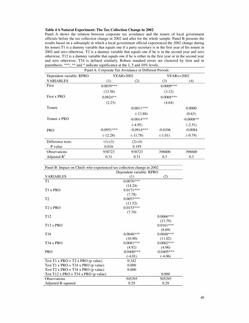
40

Table 4 A Natural Experiment: The Tax Collection Change in 2002

Panel A shows the relation between corporate tax avoidance and the tenure of local government

officials before the tax collection change in 2002 and after for the whole sample. Panel B presents the

results based on a subsample in which a local government official experienced the 2002 change during

his tenure.T1 is a dummy variable that equals one if a party secretary is in the first year of his tenure in

2002 and zero otherwise. T2 is a dummy variable that equals one if he is in the second year and zero

otherwise. T12 is a dummy variable that equals one if he is either in the first year or in the second year

and zero otherwise; T34 is defined similarly. Robust standard errors are clustered by firm and in

parenthesis. ***, ** and * indicate significance at the 1, 5 and 10% levels.

Panel A: Corporate Tax Avoidance in Different Periods

Dependent variable: RPRO YEAR>2002 YEAR<=2002

VARIABLES (1) (2) (3) (4)

First 0.0039***

0.0009***

(13.56)

(3.12)

First x PRO 0.0024**

0.0068***

(2.23)

(4.64)

Tenure

-0.0011***

0.0000

(-13.88)

(0.63)

Tenure x PRO

-0.0014***

-0.0008**

(-4.95)

(-2.51)

PRO -0.0951*** -0.0914*** -0.0106 -0.0084

(-12.28) (-11.78) (-1.01) (-0.79)

Difference tests: (1)-(3) (2)-(4)

P-value 0.016 0.195

Observations 938723 938723 398600 398600

Adjusted R2 0.31 0.31 0.3 0.3

Panel B: Impact on Chiefs who experienced tax collection change in 2002


VARIABLES (1) (2)

T1 0.0076***

(14.24)

T1 x PRO 0.0171***

(7.78)

T2 0.0057***

(11.52)

T2 x PRO 0.0153***

(7.70)

T12 0.0066***

(13.79)

T12 x PRO 0.0161***

(8.69)

T34 0.0048*** 0.0048***

(10.90) (11.02)

T34 x PRO 0.0081*** 0.0082***

(4.92) (4.96)

PRO -0.0400*** -0.0405***

(-4.01) (-4.06)

Test T1 x PRO = T2 x PRO (p value) 0.342




Observations 505295 505295

Adjusted R-squared 0.29 0.29

41

Table 5 Unexpected Official Turnovers and Corporate Tax Avoidance

This table reports results of differences-in-differences design for 22 unexpected official turnovers due

to sudden death, under investigation or dismissal from duty. The year of an unexpected turnover is

defined as year t. For each city that experienced an unexpected turnover, we identify a matching city in

the same province, with similar GDP level, and whose political leader experiences no turnover during

the period of (t-1, t+1). Change equals to one if a city experiences unexpected turnover of political

leader and zero otherwise; After equals to one if it is the event year or the following year and zero

otherwise. The definitions of all variables are in Appendix A. A constant term, year fixed effects,

province fixed effects, and their interactions with PRO are included in all regressions. Robust standard

errors are clustered by firm and reported in parenthesis. ***, ** and * indicate significance at the 1%, 5%

and 10% levels respectively.

All Unexpected Turnovers Excluding Beijing

and Shanghai

VARIABLES (1) (2) (3) (4)

Change 0.0007 0.0057*** 0.0027*

(0.62) (4.02) (1.76)

Change x PRO -0.0186*** -0.0289*** -0.0261***

(-5.35) (-6.06) (-5.30)

After -0.0045*** -0.0074*** -0.0137***

(-3.77) (-3.47) (-6.01)

After x PRO -0.0219*** -0.0442*** -0.0424***

(-5.54) (-5.97) (-5.65)

Change x After -0.0018 0.0015

(-0.69) (0.56)

Change x After x PRO 0.0568*** 0.0548***

(6.25) (5.91)

PRO -0.1006*** -0.1000*** -0.1016*** -0.0575***

(-9.60) (-9.57) (-9.72) (-6.01)

Tax x PRO -0.0740*** -0.0732*** -0.0735*** -0.0656***

(-13.64) (-13.50) (-13.56) (-11.26)

Finance x PRO 0.2277*** 0.2306*** 0.2278*** 0.1597***

(6.67) (6.77) (6.68) (4.62)

Labor x PRO 0.0131*** 0.0129*** 0.0130*** 0.0123***

(11.13) (11.01) (11.06) (9.96)

Rsales x PRO 0.1714*** 0.1708*** 0.1707*** 0.1692***

(36.99) (36.80) (36.77) (34.06)

SOE x PRO -0.0127*** -0.0133*** -0.0134*** -0.0157***

(-2.63) (-2.75) (-2.74) (-2.89)

GDPG x PRO -0.0363** -0.0349** -0.0288* -0.0104

(-2.29) (-2.20) (-1.81) (-0.57)

Tax 0.0501*** 0.0500*** 0.0501*** 0.0539***

(33.81) (33.68) (33.75) (31.76)

Finance 0.4126*** 0.4125*** 0.4140*** 0.5359***

(21.00) (21.00) (21.07) (26.22)

Labor -0.0024*** -0.0023*** -0.0024*** -0.0015***

(-7.99) (-7.93) (-7.99) (-4.59)

Rsales 0.0304*** 0.0304*** 0.0304*** 0.0273***

(33.04) (33.09) (33.08) (29.17)

SOE -0.0311*** -0.0311*** -0.0311*** -0.0328***

(-46.10) (-46.07) (-46.04) (-43.99)

GDPG 0.0186*** 0.0178*** 0.0182*** -0.0116**

(5.13) (4.93) (5.02) (-2.41)

Observations 267739 267739 267739 218612

Adjusted R2 0.36 0.36 0.36 0.39

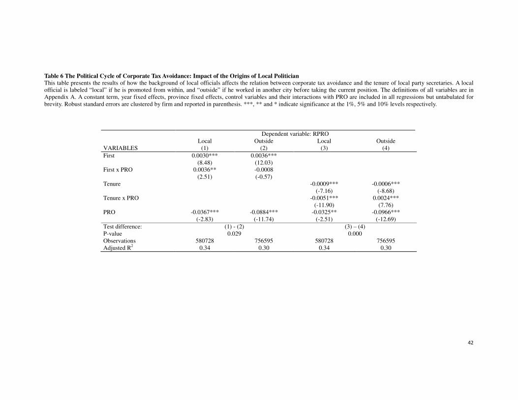
42

Table 6 The Political Cycle of Corporate Tax Avoidance: Impact of the Origins of Local Politician

This table presents the results of how the background of local officials affects the relation between corporate tax avoidance and the tenure of local party secretaries. A local

official is labeled “local” if he is promoted from within, and “outside” if he worked in another city before taking the current position. The definitions of all variables are in

Appendix A. A constant term, year fixed effects, province fixed effects, control variables and their interactions with PRO are included in all regressions but untabulated for

brevity. Robust standard errors are clustered by firm and reported in parenthesis. ***, ** and * indicate significance at the 1%, 5% and 10% levels respectively.


Local Outside Local Outside

VARIABLES (1) (2) (3) (4)

First 0.0030*** 0.0036***

(8.48) (12.03)

First x PRO 0.0036** -0.0008

(2.51) (-0.57)

Tenure -0.0009*** -0.0006***

(-7.16) (-8.68)

Tenure x PRO -0.0051*** 0.0024***

(-11.90) (7.76)

PRO -0.0367*** -0.0884*** -0.0325** -0.0966***

(-2.83) (-11.74) (-2.51) (-12.69)

Test difference: (1) - (2) (3) – (4)

P-value 0.029 0.000

Observations 580728 756595 580728 756595

Adjusted R2 0.34 0.30 0.34 0.30

43

Table 7 Alternative measure of tax avoidance

The dependent variables are effective tax rate (TAX), defined as income tax payable deflated by pre-tax

profit. TAX is zero for loss firms. We exclude the observations of Tax greater than 1. Y2002R is an

indicator variable that equals one if it is after 2002 and zero otherwise. The definitions of all variables

are in Appendix A. Year fixed effects, province fixed effects, and their interactions with PRO are

included in all regressions. Robust standard errors are clustered by firm and reported in parenthesis.

***, ** and * indicate significance at the 1%, 5% and 10% levels respectively.

Dependent variable: TAX

VARIABLES (1) (2) (3) (4)

First 0.0028*** -0.0059***

(8.77) (-8.20)

Tenure -0.0011*** 0.0003**

(-11.60) (1.99)

First x Y2002R 0.0109***

(13.40)

Tenure x Y2002R -0.0020***

(-9.84)

SOE -0.0124*** -0.0123***

(-16.57) (-16.53)

Size -0.0098*** -0.0099*** -0.0096*** -0.0096***

(-48.27) (-48.31) (-46.77) (-46.74)

Leverage -0.0208*** -0.0207*** -0.0194*** -0.0193***

(-30.85) (-30.78) (-28.47) (-28.35)

Finance 0.0237*** 0.0236*** 0.0121 0.0122

(2.67) (2.66) (1.37) (1.37)

Labor 0.0117*** 0.0117*** 0.0122*** 0.0121***

(41.79) (41.77) (43.49) (43.36)

Rsales 0.0136*** 0.0135*** 0.0142*** 0.0141***

(15.81) (15.72) (16.56) (16.46)

PCHG 0.0018*** 0.0020*** 0.0015*** 0.0019***

(4.61) (5.33) (3.99) (4.90)

Mtenure 0.0025*** 0.0027*** 0.0025*** 0.0027***

(26.02) (27.34) (25.68) (27.14)

GDPG -0.0029 -0.0028 -0.0041 -0.0036

(-1.13) (-1.11) (-1.63) (-1.42)

Constant 0.2092*** 0.2129*** 0.2090*** 0.2067***

(69.33) (70.31) (69.25) (67.50)

Observations 1337323 1337323 1337323 1337323

Adjusted R2 0.06 0.06 0.06 0.06

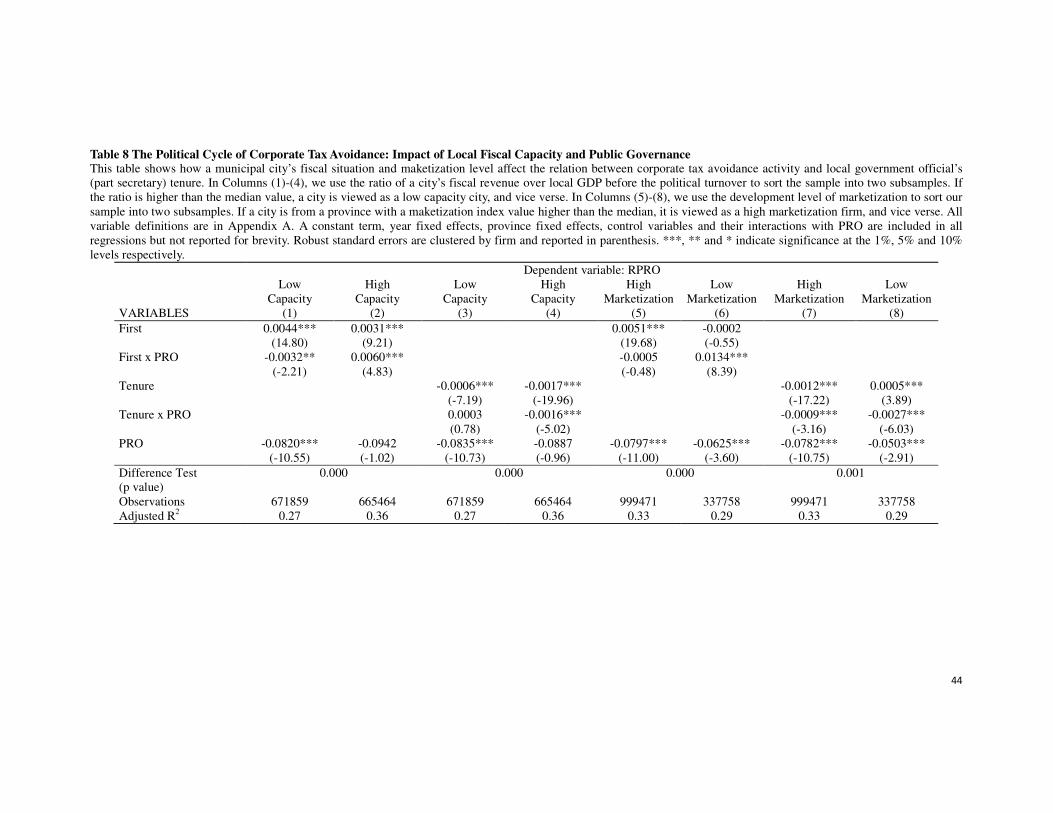
44

Table 8 The Political Cycle of Corporate Tax Avoidance: Impact of Local Fiscal Capacity and Public Governance

This table shows how a municipal city’s fiscal situation and maketization level affect the relation between corporate tax avoidance activity and local government official’s

(part secretary) tenure. In Columns (1)-(4), we use the ratio of a city’s fiscal revenue over local GDP before the political turnover to sort the sample into two subsamples. If

the ratio is higher than the median value, a city is viewed as a low capacity city, and vice verse. In Columns (5)-(8), we use the development level of marketization to sort our

sample into two subsamples. If a city is from a province with a maketization index value higher than the median, it is viewed as a high marketization firm, and vice verse. All

variable definitions are in Appendix A. A constant term, year fixed effects, province fixed effects, control variables and their interactions with PRO are included in all

regressions but not reported for brevity. Robust standard errors are clustered by firm and reported in parenthesis. ***, ** and * indicate significance at the 1%, 5% and 10%

levels respectively.


Low

Capacity

High

Capacity

Low

Capacity

High

Capacity

High

Marketization

Low

Marketization

High

Marketization

Low

Marketization

VARIABLES (1) (2) (3) (4) (5) (6) (7) (8)

First 0.0044*** 0.0031*** 0.0051*** -0.0002

(14.80) (9.21) (19.68) (-0.55)

First x PRO -0.0032** 0.0060*** -0.0005 0.0134***

(-2.21) (4.83) (-0.48) (8.39)

Tenure -0.0006*** -0.0017*** -0.0012*** 0.0005***

(-7.19) (-19.96) (-17.22) (3.89)

Tenure x PRO 0.0003 -0.0016*** -0.0009*** -0.0027***

(0.78) (-5.02) (-3.16) (-6.03)

PRO -0.0820*** -0.0942 -0.0835*** -0.0887 -0.0797*** -0.0625*** -0.0782*** -0.0503***

(-10.55) (-1.02) (-10.73) (-0.96) (-11.00) (-3.60) (-10.75) (-2.91)

Difference Test

(p value)

0.000 0.000 0.000 0.001

Observations 671859 665464 671859 665464 999471 337758 999471 337758

Adjusted R2 0.27 0.36 0.27 0.36 0.33 0.29 0.33 0.29

45

Table 9 Political Cycle of Tax Avoidance: Impact of Age and Career Concerns

This table presents the impact of local officials’ promotion incentives on the relation between their tenures and corporate tax avoidance activity in their jurisdictions. A party

secretary below 45 years old is viewed as a young chief who has strong incentives to seek further promotion. Those with age over 45 are viewed senior chiefs. Columns

(1)-(4) present the results of comparing young party secretaries and senior secretaries. A party secretary is defined as “promoted” if he or she holds a political rank higher than

that of his previous job. Columns (5)-(8) report the results of comparing those promoted party secretaries with those viewed as “non-promoted”. The definitions of all

variables are in Appendix A. A constant term, year fixed effects, province fixed effects, control variables and their interactions with PRO are included in all regressions but

untabulated for brevity. Robust standard errors are clustered by firm and reported in parenthesis. ***, ** and * indicate significance at the 1%, 5% and 10% levels

respectively.


Young

Chief

Senior

Chief

Young

Chief

Senior

Chief

Promoted Non

Promoted

Promoted Non

Promoted

VARIABLES (1) (2) (3) (4) (5) (6) (7) (8)

First 0.0052*** 0.0039*** 0.0008 0.0042***

(7.87) (16.55) (1.08) (17.99)

First x PRO 0.0131*** 0.0023** 0.0095*** 0.0024**

(5.08) (2.34) (3.21) (2.49)

Tenure -0.0015*** -0.0008*** -0.0009*** -0.0009***

(-8.67) (-12.57) (-4.79) (-13.58)

Tenure x PRO -0.0056*** -0.0009*** -0.0051*** -0.0007***

(-8.73) (-3.46) (-7.72) (-2.77)

PRO -0.0244 -0.0839*** -0.0156 -0.0811*** -0.0747*** -0.0541*** -0.0460*** -0.0799***

(-1.29) (-11.91) (-0.83) (-11.46) (-9.80) (-4.04) (-3.16) (-10.86)

Difference Test

(p value)

0.000 0.000 0.000 0.024

Observations 174030 1151563 174030 1151563 139733 1197590 139733 1197590

Adjusted R2 0.33 0.32 0.33 0.32 0.33 0.32 0.33 0.32

46

Table 10 The Effects of Firm-Level Characteristics

This table investigates how firm ownership (SOE vs. non SOE), a firm’s importance to local

government measured by the ratio of tax payable to local fiscal revenue, and firm size affect the

relation between corporate tax avoidance activity and the tenure of local officials. If the ratio of tax

payable to local fiscal revenue is higher than the median, we treat the firm as an important firm and

unimportant otherwise. If a firm has total assets larger than the median, the firm is viewed as a large

firm. The definitions of all variables are in Appendix A. A constant term, year fixed effects, province

fixed effects, control variables and their interactions with PRO are included in all regressions but

untabulated for brevity. Robust standard errors are clustered by firm and reported in parenthesis. ***,

** and * indicate significance at the 1%, 5% and 10% levels respectively.

Panel A: Party Secretary’s Tenure Measured by First


SOEs Non SOEs Important

Firms

Unimportant

Firms

Large

Firms

Small

Firms

VARIABLES (1) (2) (3) (4) (5) (6)

First -0.0002 0.0042*** 0.0050*** 0.0040*** 0.0027*** 0.0051***

(-0.57) (17.03) (11.57) (9.05) (9.89) (14.24)

First x PRO -0.0059 0.0026*** -0.0042** 0.0077*** -0.0043** 0.0048***

(-1.62) (2.75) (-2.30) (4.37) (-2.32) (4.41)

PRO -0.0434** -0.0688*** -0.0969*** -0.0907*** 0.0165 -0.0692***

(-2.48) (-9.68) (-6.69) (-5.27) (1.34) (-9.09)

Difference Test

(p value)

0.023 0.000 0.000

Observations 159180 1178143 347621 321699 667718 669605

Adjusted R2 0.23 0.30 0.32 0.33 0.32 0.31

Panel B: Party Secretary’s Tenure Measured by Tenure


SOEs Non SOEs Important Non

Important

Large

Firms

Small

Firms

VARIABLES (1) (2) (3) (4) (5) (6)

Tenure 0.0000 -0.0009*** -0.0010*** -0.0010*** -0.0007*** -0.0010***

(0.14) (-13.82) (-8.54) (-8.95) (-8.78) (-10.69)

Tenure x PRO 0.0023** -0.0013*** -0.0010** -0.0022*** -0.0007 -0.0014***

(2.18) (-5.30) (-2.21) (-4.93) (-1.40) (-5.19)

PRO -0.0503*** -0.0655*** -0.0955*** -0.0810*** 0.0166 -0.0651***

(-2.83) (-9.18) (-6.57) (-4.68) (1.34) (-8.51)

Difference Test

(p value)

0.001 0.061 0.159

Observations 159180 1178143 347621 321699 667718 669605

Adjusted R2 0.23 0.30 0.32 0.33 0.32 0.31

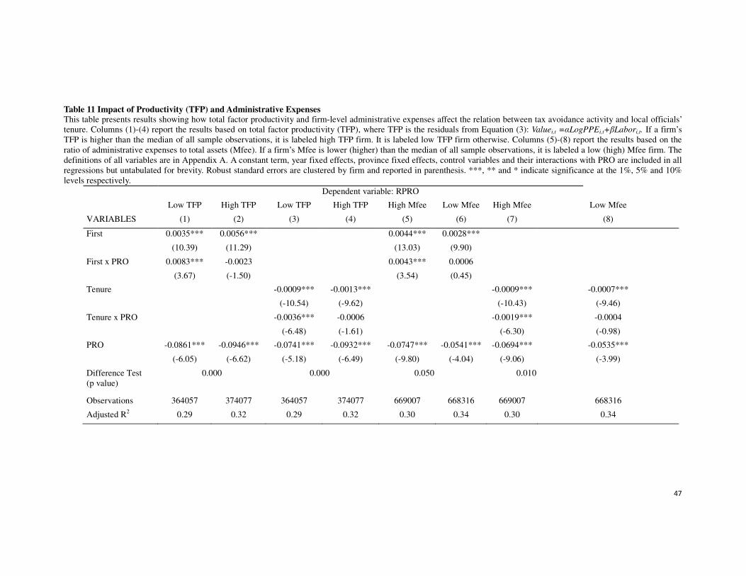
47

Table 11 Impact of Productivity (TFP) and Administrative Expenses

This table presents results showing how total factor productivity and firm-level administrative expenses affect the relation between tax avoidance activity and local officials’

tenure. Columns (1)-(4) report the results based on total factor productivity (TFP), where TFP is the residuals from Equation (3): Valuei,t =αLogPPEi,t+βLabori,t. If a firm’s

TFP is higher than the median of all sample observations, it is labeled high TFP firm. It is labeled low TFP firm otherwise. Columns (5)-(8) report the results based on the

ratio of administrative expenses to total assets (Mfee). If a firm’s Mfee is lower (higher) than the median of all sample observations, it is labeled a low (high) Mfee firm. The

definitions of all variables are in Appendix A. A constant term, year fixed effects, province fixed effects, control variables and their interactions with PRO are included in all

regressions but untabulated for brevity. Robust standard errors are clustered by firm and reported in parenthesis. ***, ** and * indicate significance at the 1%, 5% and 10%

levels respectively.


Low TFP High TFP Low TFP High TFP High Mfee Low Mfee High Mfee Low Mfee

VARIABLES (1) (2) (3) (4) (5) (6) (7) (8)

First 0.0035*** 0.0056*** 0.0044*** 0.0028***

(10.39) (11.29) (13.03) (9.90)

First x PRO 0.0083*** -0.0023 0.0043*** 0.0006

(3.67) (-1.50) (3.54) (0.45)

Tenure -0.0009*** -0.0013*** -0.0009*** -0.0007***

(-10.54) (-9.62) (-10.43) (-9.46)

Tenure x PRO -0.0036*** -0.0006 -0.0019*** -0.0004

(-6.48) (-1.61) (-6.30) (-0.98)

PRO -0.0861*** -0.0946*** -0.0741*** -0.0932*** -0.0747*** -0.0541*** -0.0694*** -0.0535***

(-6.05) (-6.62) (-5.18) (-6.49) (-9.80) (-4.04) (-9.06) (-3.99)

Difference Test

(p value)

0.000 0.000 0.050 0.010

Observations 364057 374077 364057 374077 669007 668316 669007 668316

Adjusted R2 0.29 0.32 0.29 0.32 0.30 0.34 0.30 0.34

Documents

political economy of corporate tax avoidance V2