POLITECNICO DI MILANO

Facoltà di Ingegneria Industriale

Corso di Laurea in Ingegneria Aeronautica

Ingegneria Aeronautica

MESH QUALIFICATION AND ADAPTATION BASED ON THE

TOTAL DERIVATIVE OF AERODYNAMIC FUNCTIONS W.R.T

MESH COORDINATES

Tutor: Prof. Franco AUTERI

Author:

Dario MILANI Matr. 680063

Anno Accademico 2012-2013

Acknowledgements

I would like to take this opportunity to thank the Method and Tools department in AirbusSt.Martin, Toulouse. All the components of this department contributed to the daily creationof a positive and productive atmosphere, which constitutes the main condition for any kind ofevolution, both personal and technical. I would like to thank in particular my tutor in Airbus,Renaud Sauvage, who chose me for this important project and always gave me the best baselinesin order to achieve my tasks eciently. A particular attention should be directed to MaximeNguyen-Dinh, my colleague and point of reference for the whole project. He transmitted tome all of his experience, without restriction, and contributed to the progression of my personalknowledge. Beside, these kind of contributions are often neglected, and that is why i want tohighlight to all of you who are reading this report, that without the guide and the precious helpof Maxime Nguyen-Dinh these results would not have been possible.

2

Contents

Introduction 8

1 Theory review 10

1.1 The equations of uid mechanics . . . . . . . . . . . . . . . . . . . . . . . . . . . 101.2 Gradient computation in the framework of shape optimization . . . . . . . . . . . 11

1.2.1 Finite dierences . . . . . . . . . . . . . . . . . . . . . . . . . . . . . . . . 131.2.2 Discrete direct method . . . . . . . . . . . . . . . . . . . . . . . . . . . . . 131.2.3 Discrete adjoint method . . . . . . . . . . . . . . . . . . . . . . . . . . . . 13

1.3 State of the art of mesh adaptation using the discrete adjoint method . . . . . . 141.3.1 The method of Venditti and Darmofal . . . . . . . . . . . . . . . . . . . . 141.3.2 The method of Dwight . . . . . . . . . . . . . . . . . . . . . . . . . . . . . 16

1.4 The proposed approach . . . . . . . . . . . . . . . . . . . . . . . . . . . . . . . . 161.4.1 The total derivative of aerodynamic w.r.t mesh nodes coordinates . . . . 161.4.2 Meanings of dF/dX . . . . . . . . . . . . . . . . . . . . . . . . . . . . . . 171.4.3 Mesh adaptation criteria built up from dF/dX . . . . . . . . . . . . . . . 18

1.5 Conclusions . . . . . . . . . . . . . . . . . . . . . . . . . . . . . . . . . . . . . . . 20

2 The proposed goal-oriented mesh adaptation methodology based on dF/dX 22

2.1 Denition of an adaptation sensor and a qualication criterion . . . . . . . . . . 222.1.1 Projection of dF/dX . . . . . . . . . . . . . . . . . . . . . . . . . . . . . . 232.1.2 Spatial mean . . . . . . . . . . . . . . . . . . . . . . . . . . . . . . . . . . 24

2.2 Local mesh generation and adaptation . . . . . . . . . . . . . . . . . . . . . . . . 282.2.1 Elliptic equations for mesh generation . . . . . . . . . . . . . . . . . . . . 282.2.2 Computation of P initialk . . . . . . . . . . . . . . . . . . . . . . . . . . . . 28

2.2.3 Computation of P adaptk and mesh adaptation . . . . . . . . . . . . . . . . 292.2.4 Computation and role of ε . . . . . . . . . . . . . . . . . . . . . . . . . . . 30

2.3 Conclusions . . . . . . . . . . . . . . . . . . . . . . . . . . . . . . . . . . . . . . . 30

3 Hierarchy of ve C-type grids around the RAE2822 airfoil 32

3.1 Behaviour of the mesh sensor and mesh quality criterion . . . . . . . . . . . . . . 323.1.1 The mesh quality criterion and the introduction of the average operation 32

3.2 Inuence of the number of points on the adaptation . . . . . . . . . . . . . . . . 383.3 Conclusions . . . . . . . . . . . . . . . . . . . . . . . . . . . . . . . . . . . . . . . 40

4 Application for RANS ows around the RAE2822 airfoil 42

4.1 Mesh adaptation process and software . . . . . . . . . . . . . . . . . . . . . . . . 424.2 Presentation of the steps involved in the adaptation process . . . . . . . . . . . . 43

4.2.1 CFD solver . . . . . . . . . . . . . . . . . . . . . . . . . . . . . . . . . . . 434.2.2 Post processing . . . . . . . . . . . . . . . . . . . . . . . . . . . . . . . . . 434.2.3 Adjoint vector . . . . . . . . . . . . . . . . . . . . . . . . . . . . . . . . . 444.2.4 Mesh Sensor . . . . . . . . . . . . . . . . . . . . . . . . . . . . . . . . . . 444.2.5 Grid generation and adaptation (Lama 3D) . . . . . . . . . . . . . . . . . 464.2.6 Pk eects . . . . . . . . . . . . . . . . . . . . . . . . . . . . . . . . . . . . 48

4

4.2.7 Post processing FFd72 . . . . . . . . . . . . . . . . . . . . . . . . . . . . . 494.3 2D goal function grid adaptation examples . . . . . . . . . . . . . . . . . . . . . . 51

4.3.1 Test case presentation . . . . . . . . . . . . . . . . . . . . . . . . . . . . . 524.3.2 Mesh adaptation results . . . . . . . . . . . . . . . . . . . . . . . . . . . . 52

4.4 Feature based grid adaptation . . . . . . . . . . . . . . . . . . . . . . . . . . . . . 534.4.1 Feature based adaptation theory . . . . . . . . . . . . . . . . . . . . . . . 534.4.2 Feature based adaptation example . . . . . . . . . . . . . . . . . . . . . . 544.4.3 Feature based (θgb) Vs Output based (θ) . . . . . . . . . . . . . . . . . . . 57

4.5 Conclusions . . . . . . . . . . . . . . . . . . . . . . . . . . . . . . . . . . . . . . . 58

5 3D grid local and global criteria 60

5.1 Introduction . . . . . . . . . . . . . . . . . . . . . . . . . . . . . . . . . . . . . . . 605.2 Direct and adjoint computation . . . . . . . . . . . . . . . . . . . . . . . . . . . . 605.3 Behaviour of the criterion θ . . . . . . . . . . . . . . . . . . . . . . . . . . . . . . 615.4 Conclusions . . . . . . . . . . . . . . . . . . . . . . . . . . . . . . . . . . . . . . . 64

Conclusions 66

Appendix 68

A Construction of a mesh generation elliptic system of PDEs 68

5

Nomenclature

W ow conservative variablesWb ow conservative variables extrapolated on the surfaceα vector of geometry parametrization variablesX mesh volumeF goal function as function of W and Xz goal function as function of αF goal function as function of XR residual equations as function of W and XΛ adjoint vectornβ dimension of a generic vector βf analytic uxΩ domain∂Ω contour of Ωρ uid densityu uid velocity along Xv uid velocity along Yw uid velocity along ZE uid internal energy℘ projection operatorDG,L circle in G with radius Lθi, j local sensorθ qualication criterionθ[F ] qualication criterion computed for the function Fgi,j contra-variant metric tensorxξiξj covariant metric tensorPk control functionθgb qualication criterion for gradient based adaptationC computational spaceP parameter spaceD physical spaceξξξ coordinates in the computational spacesss coordinates in the parameter spacexxx coordinates in the physical space

6

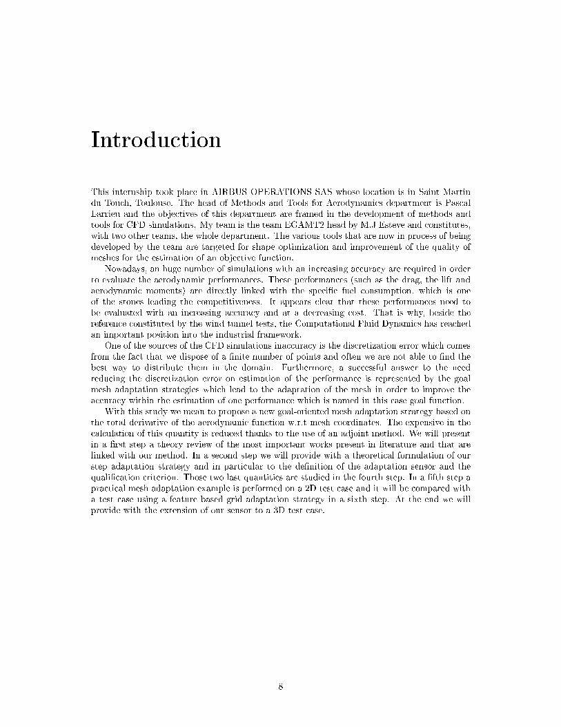
Introduction

This internship took place in AIRBUS OPERATIONS SAS whose location is in Saint Martindu Touch, Toulouse. The head of Methods and Tools for Aerodynamics department is PascalLarrieu and the objectives of this department are framed in the development of methods andtools for CFD simulations. My team is the team EGAMT2 head by M.J Esteve and constitutes,with two other teams, the whole department. The various tools that are now in process of beingdeveloped by the team are targeted for shape optimization and improvement of the quality ofmeshes for the estimation of an objective function.

Nowadays, an huge number of simulations with an increasing accuracy are required in orderto evaluate the aerodynamic performances. These performances (such as the drag, the lift andaerodynamic moments) are directly linked with the specic fuel consumption, which is oneof the stones leading the competitiveness. It appears clear that these performances need tobe evaluated with an increasing accuracy and at a decreasing cost. That is why, beside thereference constituted by the wind tunnel tests, the Computational Fluid Dynamics has reachedan important position into the industrial framework.

One of the sources of the CFD simulations inaccuracy is the discretization error which comesfrom the fact that we dispose of a nite number of points and often we are not able to nd thebest way to distribute them in the domain. Furthermore, a successful answer to the needreducing the discretization error on estimation of the performance is represented by the goalmesh adaptation strategies which lead to the adaptation of the mesh in order to improve theaccuracy within the estimation of one performance which is named in this case goal function.

With this study we mean to propose a new goal-oriented mesh adaptation strategy based onthe total derivative of the aerodynamic function w.r.t mesh coordinates. The expensive in thecalculation of this quantity is reduced thanks to the use of an adjoint method. We will presentin a rst step a theory review of the most important works present in literature and that arelinked with our method. In a second step we will provide with a theoretical formulation of ourstep adaptation strategy and in particular to the denition of the adaptation sensor and thequalication criterion. Those two last quantities are studied in the fourth step. In a fth step apractical mesh adaptation example is performed on a 2D test case and it will be compared witha test case using a feature based grid adaptation strategy in a sixth step. At the end we willprovide with the extension of our sensor to a 3D test case.

8

Chapter 1

Theory review

Nowadays a huge number of CFD simulations is steadily carried out in order to evaluate theaerodynamic performances and to improve them by shape optimization. A major cause ofthe error associated with these simulations is the discretization of the computational domainfrom which comes the interest in the research of error reduction methods by mesh adaptation.However it is not always easy to dene a process and an "indicator" to point out where and howa mesh has to be adapted in order to improve its quality. This can be intuitively implementedusing an approach based on the ow features. For example to use the static pressure gradientas an indicator for mesh adaptation. This would lead to a renement in the regions of interestcapturing shocks and vortices otherwise dumped. While these methods capture the ow featuresas described, it does not necessarily reduce the error on the desired aerodynamic functions. Thenmore useful techniques for mesh adaptation are directly based on the function of interest forexample using error estimations. Moreover these "goal-oriented" methods often use the adjointvector of the function of interest which allows to compute gradients of the functions of interestwith respect to a set of shape parameters (for shape optimization) and also with respect tovolume mesh coordinates (for mesh adaptation).

This chapter is organized as follows. The rst paragraph is a short presentation of the uidmechanics equations, the second paragraph is an introduction to the gradient computation inshape optimization framework, the third paragraph is a review of the state of the art in meshadaptation based on adjoint vector and the fourth paragraph is the presentation of the proposedmethodology.

1.1 The equations of uid mechanics

This paragraph is dedicated to the presentation of the equations that describe compressible,viscous and turbulent ows. The equations are written in the conservative form being the mostadapted form within the nite volume context.

The Euler equations

Inviscid ow are described by the Euler equations. The set of this ve equations forms a non-linear partial dierential system which can be re-written in the following Cartesian form:

∂w

∂t+ div(f) = 0, (1.1)

where w is the continuous ow eld and f is the Euler ux density:

f =

ρU

ρU⊗U + p ¯I

(ρE + p)U

,

10

where ρ is the density, U is the velocity, E is the total energy and p is the static pressurewhich has to be expressed as

p = (γ − 1)ρ(E − ||U ||2

2)

where γ is the specic heat ratio.

Navier-Stokes equations

Viscous ows are described by the Navier-Stokes equations. The conservative form of theseequations is:

∂w

∂t+ div(f − fV ) = 0, (1.2)

where

fV =

0¯τ

¯τ V − q

,

where ¯τ and q are the viscous shear stress and the heat ux respectively.

The RANS equations

At a certain Reynolds number it is observed the transition of the ow from laminar to turbulent.This transition give rise to chaotic and random processes which take place at dierent lengthand time scales. When there is a big separation between the dierent scales, the resolution ofall of them become very expensive and the cost increases with the Reynolds number. That iswhy an average of the steady Navier-Stokes equations are most often preferred.This approachconsist into the decomposition of the ow variables into a mean part and a uctuating one. Theapplication of the mean properties to the Navier-Stokes equations with this composition leadsto the RANS equations (Reynolds Averaged Navier-Stokes). However the turbulence have tobe modelled. Several turbulence model are present in the literature and the chosen one in thisframework is the one of Spalart-Allmaras [11].

1.2 Gradient computation in the framework of shape opti-

mization

This section is devoted to introduce and to provide a brief review of several methods for thecomputation of gradients that are at the basis of the developed methods in the present work.

We denote by α a vector of size nα containing the design parameters of a shape (as illustratedin Figure 1.1 where blue and red meshes correspond to two dierent values of parameter α).

The volume mesh coordinates are denoted by X, W is a vector of size nW containing theCFD solution of the problem (conservative variables at the centre of the cells) associated withthe mathematical model used and Wb is the vector containing the extrapolation of W on thesurface (Figure 1.2):

W = W (ρ, ρu, ρv, ρw, ρE)

Wb = Wb(ρ, ρu, ρv, ρw, ρE)

11

Figure 1.1: Airfoil shape and volume mesh plotted for two α values

Figure 1.2: Notations for the mesh X, the ow eld W and the ow eld on the walls Wb

We denote by R the discretized equations of uid dynamics (e.g. discrete form of Euler orRANS equations written in section 1.1) which link the elds W and the mesh X by the relation:

R(W,X) = 0,

which is a set of nW nonlinear equations.We consider a scalar function of interest, or goal, which is denoted by F . This function is

basically the lift, the drag or others quantities of interest whose computation depends on thevolume mesh X and the ow eld W . So that we can write

F = F (W,X).

This equation can also be written by highlighting the dependence on the parameter α

z(α) = z(W (α), X(α))).

Most often shape optimization methods need to evaluate the derivative of the function zwith respect to parameters α:

dz(α)

dα

The gradient can be evaluated following one of many already existing approaches whichwill be presented in the following sections (namely by nite dierences, by the Discrete directmethod or by the Discrete adjoint method).

12

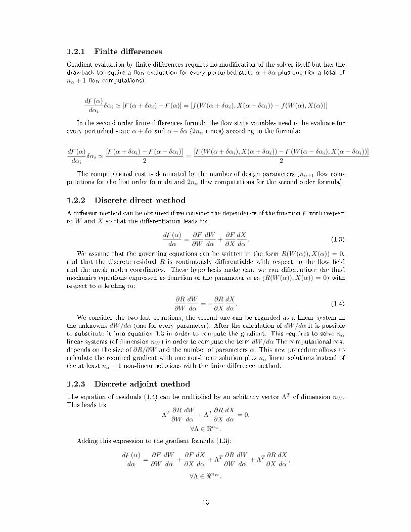
1.2.1 Finite dierences

Gradient evaluation by nite dierences requires no modication of the solver itself but has thedrawback to require a ow evaluation for every perturbed state α + δα plus one (for a total ofnα + 1 ow computations).

dz(α)

dαiδαi ' [z(α+ δαi)−z(α)] = [f(W (α+ δαi), X(α+ δαi))− f(W (α), X(α))]

In the second order nite dierences formula the ow state variables need to be evaluate forevery perturbed state α+ δα and α− δα (2nα times) according to the formula:

dz(α)

dαiδαi '

[z(α+ δαi)−z(α− δαi)]2

=[z(W (α+ δαi), X(α+ δαi))−z(W (α− δαi), X(α− δαi))]

2

The computational cost is dominated by the number of design parameters (nα+1 ow com-putations for the rst order formula and 2nα ow computations for the second order formula).

1.2.2 Discrete direct method

A dierent method can be obtained if we consider the dependency of the function z with respectto W and X so that the dierentiation leads to:

dz(α)

dα=

∂F

∂W

dW

dα+∂F

∂X

dX

dα. (1.3)

We assume that the governing equations can be written in the form R(W (α)), X(α)) = 0,and that the discrete residual R is continuously dierentiable with respect to the ow eldand the mesh nodes coordinates. These hypothesis make that we can dierentiate the uidmechanics equations expressed as function of the parameter α as (R(W (α)), X(α)) = 0) withrespect to α leading to:

∂R

∂W

dW

dα= − ∂R

∂X

dX

dα. (1.4)

We consider the two last equations, the second one can be regarded as a linear system inthe unknowns dW/dα (one for every parameter). After the calculation of dW/dα it is possibleto substitute it into equation 1.3 in order to compute the gradient. This requires to solve nαlinear systems (of dimension nW ) in order to compute the term dW/dα The computational costdepends on the size of ∂R/∂W and the number of parameters α. This new procedure allows tocalculate the required gradient with one non-linear solution plus nα linear solutions instead ofthe at least nα + 1 non-linear solutions with the nite dierence method.

1.2.3 Discrete adjoint method

The equation of residuals (1.4) can be multiplied by an arbitrary vector ΛT of dimension nW .This leads to:

ΛT∂R

∂W

dW

dα+ ΛT

∂R

∂X

dX

dα= 0,

∀Λ ∈ <nw .

Adding this expression to the gradient formula (1.3):

dz(α)

dα=

∂F

∂W

dW

dα+∂F

∂X

dX

dα+ ΛT

∂R

∂W

dW

dα+ ΛT

∂R

∂X

dX

dα,

∀Λ ∈ <nW .

13

Carrying out the term dW/dα we obtain the following relation:

dz(α)

dα= (

∂F

∂W+ ΛT

∂R

∂W)dW

dα+∂F

∂X

dX

dα+ ΛT (

∂R

∂X

dX

dα),

∀Λ ∈ <nW .

The vector ΛT (called adjoint vector) is chosen in order to annihilate the rst term of thelast equation (this fact allows to avoid the computation of the nα linear systems required forthe discrete direct method) This lead to:

∂F

∂W+ ΛT (

∂R

∂W) = 0. (1.5)

The gradient is then given by:

dz(α)

dα=∂F

∂X

dX

dα+ ΛT (

∂R

∂X

dX

dα). (1.6)

The computation of Λ (1.5) does not depend on the number of parameters nα but only onthe number of functions of interest (nF ).

The crucial point we have to point out is the signicant dierence in terms of cost between thedierent approaches. Indeed, in typical aerodynamic applications, the number of parametersis greater than number of functions (nα nF ) and then the adjoint method is most oftenpreferred to others.

1.3 State of the art of mesh adaptation using the discrete

adjoint method

Our purpose is to build a functional output grid adaptation strategy based on the adjoint vector.In literature dierent strategies have been described with the same purpose. The referenceon adjoint-based grid adaptation for functional output is the method proposed by: David A.Venditti and David L. Darmofal [15]. We can also cite the work of Richard P. Dwight [8].

1.3.1 The method of Venditti and Darmofal

Venditti and Darmofal proposed to use an adjoint formulation to relate the local residual errorin the ow solution to the global error in the chosen output thus obtaining a mesh adaptationstrategy.

This method needs two mesh levels. A coarse mesh on which CFD calculations are aordable,and a ne mesh used to generate a correction of the error of discretization (it should be notedthat CFD calculations on the ne mesh are supposed to be extremely expensive). This correctionis made up because it is possible to evaluate a part of the error. The part of the error whichis evaluable is called computable error while the non computable part is called remaining error.The computable error can be directly used to correct the functional estimation. Finally, theadaptation method is based on an estimation of the remaining error. Within the followingpassages we try to exhibit the formulation of this remaining error which is used to adapt themesh. The ow solution on a very ne grid is denoted byWh(where we suppose that the solutionis very close to the exact one) and δWh the error perturbation vector of the solution on the negrid, the expression for the perturbed direct ow solution Wh is:

Wh = Wh + δWh. (1.7)

The functional calculated over the ne grid is denoted by Fh and is evaluated on the Wh

and Wh. This lead to the following relation:

δFh = Fh(Wh)− Fh(Wh). (1.8)

14

As well as for the already dened residuals calculated over the ne grid:

δRh = Rh(Wh)−Rh(Wh) = Rh(Wh), (1.9)

where Rh(Wh) is zero by construction. Writing down the equations of the small variations ofFh and R yields:

δFh ≈∂Fh∂Wh

δWh, (1.10)

Rh(Wh) = δRh(Wh) ≈ ∂Rh∂Wh

δWh. (1.11)

Multiplying the last equation by a vector ΛTh leads to:

ΛThRh(Wh) ≈ ΛTh∂Rh∂Wh

δWh. (1.12)

Summing member to member the equations (1.10) and (1.12):

δFh +Rh(Wh) ≈ ∂Fh∂Wh

δWh + ΛTh∂Rh∂Wh

δWh. (1.13)

Which can be factorised by δWh :

δFh + ΛThR(Wh) ≈ (∂Fh∂Wh

+ ΛTh∂R

∂Wh)δWh. (1.14)

The vector ΛT is chosen such that term on the right hand side of the equation vanishes:

∂Fh∂Wh

+ ΛTh∂R

∂Wh= 0. (1.15)

With this choice of Λ, equation (1.14) leads to:

δFh − ΛThR(Wh) ≈ 0. (1.16)

We can notice that this relation correspond to (1.5) on the ne mesh. After its computation itis possible to correct the generated error in the functional Fh(Wh) by a perturbation of the owsolution Wh using the term:

δFh ≈ −ΛThR(Wh),

which is an exact expression for linear functional and residuals. The computation of the adjointvector on the ne grid is too expensive. Therefore an estimation of Λh is considered and itis expressed as we did for the residuals and the functional as the sum of the adjoint vectorcalculated on the ne grid and a perturbation δΛh

Λh ≡ Λh + δΛh. (1.17)

The perturbation on the functional of interest can be rewritten taking into account this lastrelation:

δFh ≈ ΛThRh(Wh) = ΛThRh(Wh)− δΛThRh(Wh). (1.18)

We are able now to highlight the computable correction term which is:

ΛThRh(Wh),

and the remaining error which is:−δΛThRh(Wh).

15

The expression of the remaining error will be:

δFh − ΛThRh(Wh) ≈ −δΛThRh(Wh). (1.19)

The strategy used by the authors consists in a rst step to correct the functional with

the term ΛThRh(Wh) and in a second step to use an adaptive process to further enhance thefunctional estimation accuracy by reducing the remaining error which is expressed in the right-side of equation (1.19). The elds Λh andWh represent the values of Λ andW calculated on thene mesh, as the elds ΛH and WH represent the values of Λ and W calculated on the coarsemesh. The computation of Λh and Wh is considered too expensive and approximation Λh andWh are computed by interpolation of the variables ΛH and WH over the ne grid.

The advantage of this method is that they build this correction which can be used in anycontext (scheme) but the bigger drawback is that a second very ne mesh is required with allthe complication brought about data storage and interpolation problems.

1.3.2 The method of Dwight

The method proposed by Dwight [2] is a very dierent adjoint-based method which considers thesensitivity of the functional of interest to the level of dissipation introduced by the numericalux (articial viscosity scheme with two parameters k(2) k(4) which control the dissipation).The study was eectuated on the numerical ux of the Jameson et.al. scheme ([3]). A study onseveral mesh sizes shows that more than 90% of the discretization error is due to the dissipationterms which are setted by the parameters k(2) and k(4). The expression of the discretizationerror due to dissipation is:

η = k(2) dF

dk(2)+ k(4) dF

dk(4). (1.20)

The derivatives that appear in this relation can only be computed using the adjoint methodwhich leads to:

dF

dK2= λT

∂R

∂K2

anddF

dK4= λT

∂R

∂K4

Thus the error measure can be rewritten:

η = Λ(k2 ∂R

∂k2+ k4 ∂R

∂k4), (1.21)

where it appears clearly the role of the adjoint vector. The method consist in dening thedissipation parameters for each cell:

ηi = Λ(k2i

∂R

∂k2i

+ k4i

∂R

∂k4i

). (1.22)

Intuitively it is possible to rene locally the mesh in order to minimize the dissipation errorMoreover F − k(2)dF/dk(2) − k(4)dF/dk(4) is considered as a corrected output value.

The positive aspect of this method with respect to the method implemented by Venditti andDermofal is that this method does not require a second mesh, but the most important drawbackis that it is restricted to the Jameson et. al. scheme.

1.4 The proposed approach

1.4.1 The total derivative of aerodynamic w.r.t mesh nodes coordi-nates

It has been shown in the paragraph (1.2.3) that the expression of dF/dα can be evaluated usingan adjoint approach with the following relation:

16

dz(α)

dα=∂F

∂X

dX

dα+ ΛT (

∂R

∂X

dX

dα). (1.23)

Factorising this last equation with respect to dX/dα we obtain:

dz(α)

dα= (

∂F

∂X+ ΛT

∂R

∂X)dX

dα. (1.24)

This allows to identify the expression of the total derivative of F w.r.t to mesh nodes coor-dinates:

dz(α)

dα= (

dF

dX)dX

dα. (1.25)

It can also be proved that the term into brackets of the expression (1.24) is the term (dF/dX)which compares in the expression (1.25). We notice that the totally derivative of our functionalcompares naturally in the formulation of the adjoint method, and its expression is given by:

dF

dX=∂F

∂X+ ΛT

∂R

∂X. (1.26)

This derivative is the starting point of our work.

1.4.2 Meanings of dF/dX

The derivative dF/dX is a link between the functional F and the volume mesh X so it gives usessential information for the mesh adaptation. As it indicates the sensitivity of the functionaloutput with respect to the volume mesh (Figure 1.3), this variable is calculated for every pointof the grid and it denes the inuence of these points position on the goal estimation.

Figure 1.3: Example (dCdp)/(dX)

The equation (1.26) is composed by two terms:

dF

dX=

∂F

∂X︸︷︷︸geometrical derivative

+ ΛT∂R

∂X︸ ︷︷ ︸aerodynamic derivative

. (1.27)

17

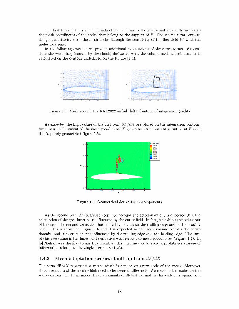
The rst term in the right hand side of the equation is the goal sensitivity with respect tothe mesh coordinates of the nodes that belong to the support of F . The second term containsthe goal sensitivity w.r.t the mesh nodes through the sensitivity of the ow eld W w.r.t thenodes locations.

In the following example we provide additional explanations of these two terms. We con-sider the wave drag (caused by the shock) derivative w.r.t the volume mesh coordinates. It iscalculated on the contour underlined on the Figure (1.4).

Figure 1.4: Mesh around the RAE2822 airfoil (left); Contour of integration (right)

As expected the high values of the rst term ∂F/∂X are placed on the integration contour,because a displacement of the mesh coordinates X generates an important variation of F evenif it is purely geometric (Figure 1.5).

Figure 1.5: Geometrical derivative (x-component)

As the second term ΛT (∂R/∂X) keep into account the aerodynamic it is expected that thecalculation of the goal function is inuenced by the entire eld. In fact, we exhibit the behaviourof this second term and we notice that it has high values on the trailing edge and on the leadingedge. This is shown in Figure 1.6 and it is expected as the aerodynamic couples the entiredomain, and in particular it is inuenced by the trailing edge and the leading edge. The sumof this two terms is the functional derivative with respect to mesh coordinates (Figure 1.7). In[5] Nielsen was the rst to use this quantity. His purpose was to avoid a prohibitive storage ofinformation related to the singles terms in (1.26).

1.4.3 Mesh adaptation criteria built up from dF/dX

The term dF/dX represents a vector which is dened on every node of the mesh. Moreoverthere are nodes of the mesh which need to be treated dierently. We consider the nodes on thewalls contour. On these nodes, the components of dF/dX normal to the walls correspond to a

18

Figure 1.6: Aerodynamic derivative (x-component)

Figure 1.7: Complete derivative (x-component)

change of the shape. Than we introduce a projection (which we will call as ℘) of dF/dX whichdoes not mean to change the shape of the airfoil and is dened by:

℘(dF/dX) = dF/dX In the volume℘(dF/dX) = dF/dX − (dF/dX · ~n)~n Along the walls contour℘(dF/dX) = 0 At the corner of the walls

This projection is introduced in order to maintain only the components of dF/dX (Figure1.8) that are actually usable for mesh adaptation. A Taylor series at the rst order gives:

F(X + dX) ' F(X) +dF

dXdX

By applying the projection we also get:

F(X + dX)− F(X) ' ℘(dF

dX)dX

A majoration of the right hand side of this expression can be computed. This is obtained byconsidering that the admissible mesh displacement dX is such that each node is to stay in acircle of radius half the distance to its closest neighbour. Our criterion is now able to takeinto account the already existing distance between those nodes so that we will displace them inagreement with the "room" at disposition.

In addition to this local criterion we introduced a global one, which allows to dene theglobal quality of the mesh. All the explanations and developments will be given in the following

19

Figure 1.8: dF/dX projection

chapter. We notice that the rst use of dF/dX for mesh adaptation have been done by Peteret. al. in [7] for 2D and 3D Euler ow computations.

1.5 Conclusions

This chapter gave a review about the dierent strategies which can be found in literature whichuse the adjoint methods to reduce the error associate with a computation of a functional F. Afterthat we introduced the basic idea of our method which is close to the Venditti and Dermofal [15]one but is quite dierent in respect to the method implemented by Dwight [2]. The importantadvantage of our method is that it does not depend on the scheme used as for Dwight method,and it does not require two levels of mesh as for the method implemented by Venditti andDermofal. The adjoint is calculated because it serves to compute the sensitivity dF/dX. Ourpurpose is to use this sensitivity as indicator for our mesh adaptation strategy as we explain inthe following chapter.

Furthermore our method uses the variable Λ which is also often used in shape optimizationframework. This fact lead undoubtedly to computation time saving because Λ would be alreadygiven and it would not require further computations.

20

Chapter 2

The proposed goal-oriented mesh

adaptation methodology based on

dF/dX

This chapter is devoted to the theoretical presentation of the sensor built up from dF/dX andthe mesh adaptation strategy used for practical applications. First of all the local sensor (whichwill be used to induce the adaptation of the mesh) and the global one (which is used as indicatorof the global mesh quality) are presented. In a second step the mesh adaptation strategy basedon an elliptic PDE is presented.

2.1 Denition of an adaptation sensor and a qualication

criterion

The previous chapter introduced the total derivative of the function of interest w.r.t meshcoordinates (1.26). As this derivative indicates the sensitivity of the goal function F w.r.t thevolume mesh X, we can intuitively state that it tends towards zero when the mesh is ideallyadapted for the calculation of F. This condition can be achieved only in the case of innitygrid renement, so it is clear that we have to use the sensitivity dF/dX in a dierent way. Weexplain within this section the considerations which bring us to the theoretical denition of theadaptation sensor and the qualication criterion.

The rst consideration which has to be taken into account is about stability. We takea volume mesh denoted by X and a second mesh volume which is a perturbed state of therst one, which is denoted by X + dX. The ow state variables computation (W ) allows thecomputation by integration of a goal function F. This goal function can be the lift coecient,the drag coecient or others quantities of interest for the both initial mesh and perturbed mesh:

X F(X)X + dX F(X + dX)

The mesh X is considered to be at a stable position if F(X + dX) - F(X) is small. Thisfact means that for a perturbation of the mesh nodes position, the functional calculated doesnot change signicantly. In fact, a condition which is necessary for a good mesh quality is thatits perturbation does not play an important role in the calculation of the solution, because itwould not have physical reasons as the boundary conditions would not change.

It is necessary to consider that on the solid contours the inuence of the perturbation dXalong the normal direction of the solid contours has physical reasons to change the evaluation ofthe functional F(X + dX) as it represents a change of the solid shape. This consideration leadsto the introduction of the projection operator ℘ in paragraph 2.1.1, and the correct formulation

22

of the stability condition has to delete the components of dF/dX that change the shape. Westate as consequence that for a volume mesh denoted by X and a second volume mesh which isa perturbed state of the rst one, which is denoted by X + dX. The mesh X is considered astable position if ℘(F(X + dX)) - ℘(F(X)) is small.

The attempt towards the stability condition is made by trying to pull dF/dX towards zero,but in a discretized context where a redistribution of point it is necessary to improve the accuracyof the goal function estimation without increasing the number of nodes and the calculation time,it is preferable to redistribute the points trying to reach a situation in which the sensitivitydF/dX is the same along the mesh.

Moreover, in a structured mesh context, where the regularity is one of the crucial points, itis preferable to weight the sensitivity by a characteristic length ri,j . Thanks to ri,j it is possibleto take into account that on the zones where the mesh is already ne, an important sensitivityof dF/dX would induce a strong irregularity, so a smaller mesh points movement is allowed.

In the following we mean to explain the practical aspect which stands with the previousconsiderations, especially on the projection operator and the characteristic length which lead tothe denition of the sensor and the qualication criteria.

Roughly speaking, the multiplication by a characteristic length assures that the sensor willbe able to take into account the importance of the mesh displacement on the calculation of Fweighted by the local size of the mesh. If we achieve a reduction of this criterion we also achievethe best distribution of points to calculate F.

2.1.1 Projection of dF/dX

As we explained in section 1.4.3, close to the wall a displacement of the grid would lead to adeformation of the wall geometry. A projection operator has therefore been devised to avoidany deformation of the body shape and it will be denoted by ℘(dF/dX)dX (Figure 1.8) in whatfollows. This operator should preserve the displacement of the internal points while avoidingany movement of the boundary points that would deform the body shape, additional details willbe given in the following. The projection is represented in Figure 2.1 where the eect of theprojection on the displacement of a point lying on a solid surface is illustrated. It is clear thatthe points on the skin can move only along the solid surface. The projection is dened throughthe operator on which the goal sensitivity acts as:

℘(dF

dX)dX. (2.1)

Figure 2.1: dF/dX projection

Since a given grid does not, in general, allow a complete resolution of the physic of theproblem which is necessary for an accurate computation of a given output, ℘(dF/dX)dX willbe highly discontinuous especially at the rst step of adaptation as shown in Figure 2.3.

In order to partially supply at this fact it is possible to introduce a spatial-mean which willbe furthermore studied in section 2.1.2.

23

Denition of the global and the local criteria of mesh quality

We denote by ri,j half the distance between the grid point Xi,j and the closest one. This leadsto the formal denition of our qualication criterion θ as follows:

θ(i, j) = ‖℘(dF

dX)i,j‖ ri,j , (2.2)

An example of the θ(i, j) eld is reported in Figure 2.2

Figure 2.2: θ[Clp] around the RAE2822 airfoil

A global quality criterion is dened as:

θ =1

NiNj

∑i;j

θ(i, j). (2.3)

The local criterion, equation (2.2) gives information about the local quality of the grid and ithas high values on the nodes whose relocation would cause a large variation of the output. Theglobal criterion, equation (2.3) is built as the average of the local criterion on the whole domainand it is useful to evaluate the quality of the entire mesh. High values of θ mean that the pointrelocation has a high impact on the function and therefore the mesh should be adapted.

Additional explanation about the development of this sensor will be given in the followingsection.

2.1.2 Spatial mean

In this paragraph we will discuss about the tool we used to smooth the eld ℘(dF/dX). Thispoint is very important because it allows to obtain a more uniform eld which is more usefulto capture the regions where a grid modication would have an important impact on the com-putation of F . Otherwise it would not be possible to distinguish them clearly as ℘(dF/dX) ishighly irregular (Figure 2.4, left). Furthermore a smoothing is necessary because there might benodes close to each others with vectors pointing in opposite directions as illustrated in Figure2.3. This fact would cause a local compensation eect in and the nodes would be moved withoutany advantage. The smoothing is obtained by a ltering of the ℘(dF/dX) function.

The lter is in fact a weighted average. The ltered value on a grid point is computedby weighted average of the values on the points lying in its neighbourhood. It is possible toconsider neighbourhoods of dierent radius so that the ltered value of ℘(dF/dX) over a nodeis obtained taking into account a variable number of nodes around him. The neighbourhood

24

Figure 2.3: (Left) large regular ℘(dF/dX) with a large node displacement possibility; (Center)large regular ℘(dF/dX) without large possible displacement of the nodes; (Right) large irregular℘(dF/dX) with large possible displacement of nodes

Figure 2.4: Example of discontinuities of d(Cdp)/dX (Left); Regularization of d(Cdp)/dX ob-tained by ltering (Right)

radius (L) is dened in percentage of characteristic length such as the cord of the airfoil. Thesmoothing eects obtained by this operation are shown on Figure 2.4 (Right).

The choice of L has to be made as a compromise among dierent requirements such as thedegree of regularity required, the complexity of the problem geometry, the computational cost,and so on. A direct comparison of computations made with study with dierent radius has beenperformed in order to highlight issues and to evaluate the impact of the radius on the computedqualication criteria.

In the following example θ1 = θ1[Clp] and θ2 = θ2[Cdp] are the two goal functions chosen.The calculation is performed on the RAE2822 airfoil, the Reynolds number is Re=6.5 106, theMach number isM∞ = 0.725, the angle of attack is α = 2.466 and a Spalart-Allmaras turbulencemodel has been employed. The calculation was performed on a structured grid (Figure 2.5) usingan upwind-scheme (Roe scheme).

25

Figure 2.5: Mesh around the RAE2822 airfoil

The ow solution is plotted for the Mach number variable in Figure 2.6. The θ1 and θ2 builtfor dierent values of the radii L are plotted in the Figure 2.7 and 2.8 respectively.

Figure 2.6: Mach around the RAE2822 airfoil

It can be observed that the criterion θ calculated for Clp and Cdp detects the zones whichhave to be adapted in order to reduce the inuence of the mesh on the calculation of these twoobjective functions. The criterion is plotted in Figure 2.7 for Clp and in Figure 2.8 for Cdpfor increasing radii. When L = 0 and the lter is not applied the gure shows that the zonesdetected are the shock wave, the trailing edge and the leading edge as others methods for meshadaptation would detect. As usual in mesh adaptation literature a comparison with the featurebased adaptation method is performed. This comparative highlights that our method detectszones of the domain which would not be detected from a feature-based method. An importantexample consists in the detection of the upstream zone. That region is detected because the

26

Figure 2.7: Quality criteria for Clp, θ1: without average, L = 0,L = 0.2,L = 0.4,L = 0.8

Figure 2.8: Quality criteria for Cdp, θ2: without average, L = 0,L = 0.2,L = 0.4,L = 0.8

proposed method because this criterion is able to predict that the error associated with the owcomputation are transported along the ow eld by advection, so that the errors introducedalong the inlet boundary are transported up to the airfoil generating an inaccurate estimate ofthe goal F .

Furthermore the importance of a good accuracy on the upstream is underlined by lookingat the gures generated for increasing values of L. The criterion is plotted for L = 0.2, L = 0.4and L = 0.8. It is clear that the renement of the mesh in the upstream region becomes moreimportant with respect to the region around the shock. Evidences of this fact will be given inthe Section 4.4 where the numerical solution is compared with experimental results.

It can be observed that θ decreases while the radius increases. Furthermore, the criterionpredicts a better global mesh quality when the average is taken. This fact is due to the chosenltering operator which has the eect of smoothing the zones containing high values of dF/dX.This is a positive aspect because as it allows to deal with a regular eld which is a crucial pointin the adaptation process, in particular for structured meshes. The unltered eld θ contains all

27

the information linked to the sensitivity of the function of interest with respect to the volumemesh. Of this information we choose to retain just the smooth part in order to adapt the mesh.

2.2 Local mesh generation and adaptation

The tools presented in this chapter are general. In fact they can be employed for any type ofgrid. A crucial point in the adaptation process is the smoothness and regularity of the mesh.Elliptic equations are often used for mesh generation [12] because of their high regularity.

2.2.1 Elliptic equations for mesh generation

We will refer to three dierent vector spaces with their respective coordinate systems: the rstone is the computational space with coordinates ξξξ. The second one is the parameter space withcoordinates sss. The third one is the physical domain with coordinates xxx. The coordinates inthe physical space can be considered as a function of the coordinates ξξξ. This lead towards thedenition of the following form of PDEs:

3∑i,j=1

gijxξiξj +

3∑k=1

gkkPkxξk = 0. (2.4)

Where x is the position vector (in the Cartesian reference), x = (x1, x2, x3), ξi = (ξ1, ξ2, ξ3) arethe curvilinear coordinates and gij(i, j = 1, 3) is the contra-variant metric tensor and nally Pkare the control functions. There is a unique link between the generated mesh and the controlfunctions. For example once we generate the grid it is possible to associate to it the vector ofcontrol functions (P initialk ) and vice versa (it is possible to show that we can always calculateit, even if the starting mesh does not come from a PDEs system resolution). In fact it is alsopossible to associate a modication of the control functions of a mesh, keeping the regularity ofthe initial mesh, and to adapt it.

A good method to adapt a mesh is to suitably modify the control functions and then re-compute the mesh coordinates corresponding to the new control functions. The success of thismethod relies on the way this modication is preformed. In this work, we used the informationrelated to the local criterion θi,j . The variation of control function can be expressed in generalas follows:

Pk = P initialk + εP adaptk . (2.5)

Where P adaptk are the modied control functions that will be presented in 2.2.2, P initialk are theinitial control functions used to generate the initial mesh, and ε is a parameter which controlsthe magnitude of the modication to the original mesh. More details about these quantities willbe given shortly. For the moment we underline the regularity of the generated grid which makesthese equations interesting to us. Elliptic equations present in general a high regularity whichleads to the fact that a small perturbation of the control functions induces a perturbation onall the nodes of the mesh. In Figure 4.1 the value of the function has been perturbed in a singlegrid node and it can be observed how the modication aects all the eld.

2.2.2 Computation of P initialk

The adaptation process developed in this project requires an initial mesh. For every givenmesh, the computation of P initialk coecients is possible according to the 3x3 system in (2.4)in unknowns Pk. This system has one real solution, and its solution is inexpensive but it mustbe carried out for every mesh node. Once P initialk has been computed it is possible to adapt by

adding a perturbation to the initial control functions by P adaptk which takes into account thelocal information about the need of renement. The correspondent mesh coordinates X of theadapted grid are now the non-linear unknowns of the equation 2.4, as will be made clearer inthe next section.

28

2.2.3 Computation of P adaptk and mesh adaptation

Let us focus now on the calculation of P adaptk . This could be done for instance according tothe method proposed by Soni et. al. ([10]) which is based on the state variables in order

to capture ow features as shocks. Instead, the computation of P adaptk for our purposes isperformed exploiting the information provided by the local θi,j sensor. With this section we

mean to explain how the local θi,j sensor can be used to compute P adaptk .We start by considering si : X → [0, 1](i = 1, 2) elds. Each eld si is associated to a

geometric direction and it assumes large values in areas where the mesh needs to be rened.The denition of si depends on the criteria selected by the author. For Soni et al.[10] theeld si was the component of the gradient of the Mach number in the direction i. We insteadcompute the eld si from the component of ℘(dF/dX)r in the i direction. So, the component of℘(dF/dX)r in every i direction is ltered and it is divided by the maximum value of ℘(dF/dX)r.These operations of ltering and division lead to the denition of a eld for every topologicaldirection whose values stay between -1 and 1. We dene this eld as si.

The eld si is then used to compute a eld s which compresses in one eld the informationconnected to the dierent directions (present in each eld si). Soni et al. built up s in [10] asfollows:

s = 1 + s1 ⊕ s2 ⊕ s3. (2.6)

where the symbol ⊕ represents the Boolean sum (a1 ⊕ a2 = a1 + a2 − a1a2) and it is useful inthis context because it has the propriety to exhibit high values if one of its arguments has ahigh value.

The eld s is computed starting from si elds and it is shown in (Figure 2.9). We highlightthat the dierence with respect to the method proposed by Soni. et. al. is that si in the presentcase is directly linked to the adaptation sensor.

Figure 2.9: The eld s is plotted for NACA0012, Re=∞ and Mach< 0.7 during the adaptationbased on the Cd

Finally the control functions P adaptk are dened as the derivative of this scalar eld s respectto each topological direction:

P adaptk =sξks. (2.7)

The eld s is built in order to achieve values between 1 and 2 and so that the topologicalderivatives stay between 0 and 1. It follows that the variable P adaptk is always well dened. In ourframework the si dened above corresponds to the norm of ℘(dF/dX) times the characteristiclength in the ith geometrical direction.

It has to be noticed that in practice, the highest values of P adaptk are signicantly above theaverage. This is due to two main aspects. In fact, for coarse grid the regularity of the solutionis not guaranteed while it is as the mesh size increases and the cell length tends towards zero(a demonstration is given in the [7] for Euler ows).Consequently it is necessary to smooth the

29

Figure 2.10: (Left) derivative P adapt along i topological direction; (Right) derivative P adapt

along the j topological direction

sensor in order to avoid those strong discontinuities and the necessity to introduce a cut-o inorder to partially supply at the high dispersion of the function around its average (details will be

presented in the paragraph 4.2.6). The gure 2.10 shows P adapti P adaptj which are respectivelythe criteria along the topological i and j directions built for a simple Euler-compressible case.

After these operations it will be possible to adapt the mesh according to the directionsidentied as 'important' by the sensor (Figure 2.11).

Figure 2.11: (Left) initial mesh; (Right) adapted mesh towards the directions calculated (redvectors)

2.2.4 Computation and role of ε

In agreement with equation (2.5), the proposed method employs the functions P adaptk in ordercompute the modied control function Pk used to generate the mesh according to equation (2.4).

The contribution of P adaptk to Pk is tuned by the scalar parameter ε. Dierent tests havebeen performed to calibrate this parameter. It is trivial to observe that:

• if this quantity tends towards zero, mesh will not be modied.

• if this quantity increases, a big modication is obtained.

Therefore ε controls the impact of the sensor at every adaptation step. The choice of thisparameter is crucial. In fact, it has to be computed as a compromise between convergencespeed (the smaller values of this parameter the larger number of iterations are required) andthe condence on the sensor θ Furthermore, important values of ε have to be avoid also becauseimportant modications are linked with the possibility to create folding near critical mesh points.

2.3 Conclusions

In this chapter we gave some details about the proposed adaptation strategy.

30

In the rst section we explained how we built the adaptation sensor and the qualicationcriterion starting from dF/dX. It was explain in this section that the adaptation criterion isable to take into account when there are regions of the mesh which are already very rened withrespect to others. It has also been explained how the average operator allows to improve theperformance of our sensor.

The second section meant to explain how the adaptation sensor is used to compute theadapted the mesh. With this purpose it was explained that the adaptation sensor is used tobuild the control functions P adapti which, as well as the adaptation sensor has high values inthe regions which have to be rened. P initiali are instead the control functions associated to the

initial mesh. Then, P initiali and P adapti are used to compute the new control function in accordto the equation (2.5). After the computation of the new control functions we showed how tocompute the adapted mesh in accord with elliptic equations.

31

Chapter 3

Hierarchy of ve C-type grids

around the RAE2822 airfoil

The goal-oriented mesh adaptation based on dF/dX was already applied to the solution ofEuler equations in [7]. In this paper the authors showed important properties of the presentgoal-oriented method which are now extended to the RANS equations in this work. Beforeshowing a complete adaptation loop, which will be presented in chapter 4, it is interesting toanalyse the behaviour of θ on a hierarchy of ve grids. First, we will discuss the θ-sensorproprieties (paragraph 3.1), afterwards we will focus on the properties of the adaptation process(paragraph 3.2).

3.1 Behaviour of the mesh sensor and mesh quality crite-

rion

With this paragraph we give a practical example. The denition of the sensor has been done insection 2.1. There the formulation of the local θi,j criterion and of the global θ criterion. Thelocal criterion θi,j is a sensor which is formulated to detect the mesh zones whose sensitivity onthe calculation of the goal F is important and the global criterion θ is useful to evaluate thequality of the entire mesh and his attitude for computing the goal function.

3.1.1 The mesh quality criterion and the introduction of the averageoperation

It is interesting to study the behaviour of the sensor on a hierarchy of grids in which we knowa priori what is the level of qualication. We know a priori that among the ve meshes with thesame topology the quality of the grid increase with the level because for each level the numberof nodes in each topological direction is multiplied by two. It is known that the error associatedwith the computation of the solution decreases with the decreasing of the dimensions of thecells. This lead to the fact that if the geometry is not modied the error associated with theestimation of the function F chosen will decrease as we move towards grid more rened.

As it can be observed in table 3.1, when the grid quality increases, θ decreases by aboutone order of magnitude so the correlation between the sensor θ and the quality of the grid isveried. The functions chosen in this example are the drag coecient F = Cd whose sensor isθ1 and the lift coecient F = Clp whose sensor is θ2.

It can be observed from the table 3.1 that the criterion implemented has a good correlationwith the accuracy of the computation of F . The reduction of θ is due to the reduction of theboth terms dF/dX and ri,j . This last variable is reduced on every point of a factor two alongthe hierarchy while θ decreases of about one order of magnitude. This is enough to conrmthat globally the sensitivity of F to the mesh displacement dX is smaller for the ne grids.

32

Table 3.1: Validation of the θ criterion on a mesh hierarchy (The symbol * means that thecomputation is retained to be too expensive)

Level number of nodes Cd Clp θ1 ∗ 10−7 θ2 ∗ 10−7 θ1 ∗ 10−7 θ2 ∗ 10−7

1 34 848 142.61 0.71837 41.265 61.380 28.659 40.3692 135 200 123.93 0.73950 5.0184 7.7841 3.3888 5.22503 532 512 118.77 0.74988 0.8271 1.0175 0.5411 0.66934 2 113 568 118.33 0.75445 0.1861 0.1553 0.1344 0.09575 8 421 408 118.29 0.75583 0.0465 0.0203 * *

That show the eciency of this global sensor to detect if a mesh is more reliable or not for thecalculation of an objective function.

It has to be said that all the nonlinear eects are not taken into account. The criterionis in fact based on a rst order Taylor expansion of the functional F , so the lost of a perfectcorrelation is due to the fact that the functional F is a non linear function of dX. Furthermore,as we took a rst order approximation, there are second order eects which we are not able totake into account.

About the local sensor, it has to be veried that the local criterion is able to detect therelative sensitivity of the mesh zones in every grids and that this sensitivity. We also expectthat it assumes important values in the same zones for all the grids of a given hierarchy. Onceagain, the lost of a perfect correlation between the accuracy of F and θ is attributable to thenon linearity of the functional F .

We mean now to investigate the behaviour of the local criteria into the details.

The mesh adaptation sensor and the introduction of the average oper-ator

In section 2.1 we introduced both global and local criterion. Furthermore the criterion detectsa better estimation of the second goal function with the increasing number of points and theirvalues along the mesh are less important and the estimation of the functions actually reach hislimiting values.

We will plot now the θi,j-criterion eld within the hierarchy of meshes we have used for thevalidation. The mesh hierarchy is shown on Figure 3.1, and the θ criterion is shown in theFigures 3.2 and 3.3 respectively for F1 = Cd and F2 = Clp.

The colour-map used is based on the global criterion for the two functions along the iteration.It follows that it is possible to visualize the zones with an important sensitivity with respect tothe global quality of every single case in order to point out for every grids which are the relativeimportant zones detected.

It can be checked that for every function the zones detected are the same (for all the meshes).This fact is veried because the topology is the same so even if by adding points we achieve abetter global quality, the geometry has to be adapted "in the same manner" in order to achievea better performances on the estimation of the goal without increasing the number of points, sothe calculation time. The natural consequence of this fact is the attempt to adapt the mesh. Animportant remark is that, roughly speaking, the redistribution of the points accordingly withthis sensor will not pretend to get better the prediction of the global ow solution but it willcertainly allow the best use of CPU and memory in order to compute the goal F .

With the knowledge of the behaviour within a mesh renement we can now spend a fewwords to explain why those zones are detected. So we focus for instance on the third hierarchymesh level. As it can be noticed in Figure 3.4 the main zones detected for the both function Cland Cd are: The upstream, the shock, the trailing edge,the boundary layer and a zone over theshock. Naturally the magnitude of the local θi,j is dierent for the two functions but it has thesame magnitude order.

33

Figure 3.1: Mesh hierarchy

34

Figure 3.2: Criterion θ1 plotted on the mesh hierarchy

35

Figure 3.3: Criterion θ2 plotted on the mesh hierarchy

36

The mesh is a structured multi-block mesh and is not uniform (see Figure 3.1). The com-putation of our sensor on this mesh allows the visualization of the following main zones:

Upstream

Figure 3.4: Criterion θ1 near eld region

The upstream is detected as the transport of numerical errors by advection would aectall the ow eld. The upstream zone should be more rened in order to solve all the restdownstream. It is known that a criterion based on the features of the ow would not considerthis fact as we will show in the section dedicate to the feature based adaptation.

Shock

The shock is detected (Figure 3.5) as it contains strong gradients and a coarse grid in this zonewould provoke an increasing of the dissipation so a rough resolution in term of estimation ofboth θ1 and θ2. The criterion suggests (qualitatively in accordance with the feature based) abetter renement of this zone.

Figure 3.5: Criterion θ1 around the shock

Zone over the shock

The detection zone over the shock which is shown in Figure 3.6 is due to the fact that in thiszone the gradients are still important for the computation of the functions but the mesh givenis coarse in this zone by construction. The criterion exhibit that the discontinuity in this zoneshould be avoided so a renement in this zone is necessary in order to attenuate the numericalerror dues to the rough resolution of the gradients.

37

Figure 3.6: Zone over shock, θ1 criterion plotted

Boundary layer

The boundary layer is a question a little bit more delicate. The boundary layer is turbulent andthe method suers of a lost in precision of the gradients calculated in this zone. This lost inprecision is due to the fact that for the resolution of the adjoint equation, and in particular forthe derivation of the term ∂R/∂W the thin layer and xed turbulent viscosity hypothesis aretaken into account (recent works at Onera are trying to provide the method with a completelinearisation of ∂R/∂W but for instance no work is concluded). The hypothesis play a marginalrole on our adaptation process but they would be very important within the attempt to adaptvery rened meshes.

Trailing edge

The trailing edge is an important zone within this context because the function θ exhibits highvalues. This is common to all adaptation process as well as the feature based. Numerical aspectsand relative importance of the both θ1 and θ2 have been considered and treated in the chapter4.

3.2 Inuence of the number of points on the adaptation

With this paragraph we mean to study the eect of the adaptation method on an hierarchy ofgrids. The method just implemented was designed with the goal of generality. In fact it hasto be proved that this method works with every grid and in particular that it is robust. Weobtained a prove of this propriety thanks to an adaptation on three mesh renement levels. Thisfact serves to show that in all the cases our method is reliable and robust so that it will tend toadapt the mesh with respect to the goal function for every given mesh.

Cd adaptation

Table 3.2: 1st level Cd adaptation

Iteration Cd ∗ 10−4 Clp θ1 ∗ 10−7 θ2 ∗ 10−7

0 142.61 0.71837 28.659 40.3691 133.90 0.73475 22.552 35.4282 133.75 0.73478 22.480 36.7993 133.49 0.73288 21.861 35.713

38

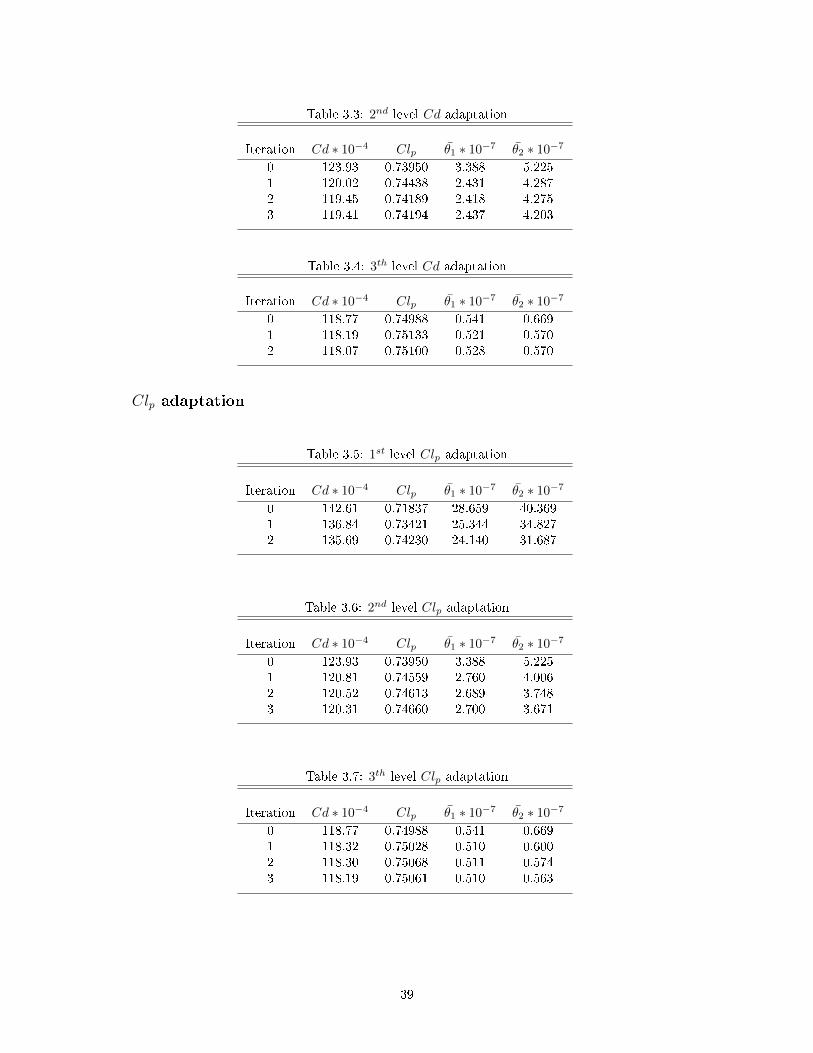
Table 3.3: 2nd level Cd adaptation

Iteration Cd ∗ 10−4 Clp θ1 ∗ 10−7 θ2 ∗ 10−7

0 123.93 0.73950 3.388 5.2251 120.02 0.74438 2.431 4.2872 119.45 0.74189 2.418 4.2753 119.41 0.74194 2.437 4.203

Table 3.4: 3th level Cd adaptation

Iteration Cd ∗ 10−4 Clp θ1 ∗ 10−7 θ2 ∗ 10−7

0 118.77 0.74988 0.541 0.6691 118.19 0.75133 0.521 0.5702 118.07 0.75100 0.528 0.570

Clp adaptation

Table 3.5: 1st level Clp adaptation

Iteration Cd ∗ 10−4 Clp θ1 ∗ 10−7 θ2 ∗ 10−7

0 142.61 0.71837 28.659 40.3691 136.84 0.73421 25.344 34.8272 135.69 0.74230 24.140 31.687

Table 3.6: 2nd level Clp adaptation

Iteration Cd ∗ 10−4 Clp θ1 ∗ 10−7 θ2 ∗ 10−7

0 123.93 0.73950 3.388 5.2251 120.81 0.74559 2.760 4.0062 120.52 0.74613 2.689 3.7483 120.31 0.74660 2.700 3.671

Table 3.7: 3th level Clp adaptation

Iteration Cd ∗ 10−4 Clp θ1 ∗ 10−7 θ2 ∗ 10−7

0 118.77 0.74988 0.541 0.6691 118.32 0.75028 0.510 0.6002 118.30 0.75068 0.511 0.5743 118.19 0.75061 0.510 0.563

39

3.3 Conclusions

With this chapter we have been able to give numerical evidences about the local sensor andthe global qualication criteria. Furthermore we showed in the rst paragraph that the globalqualication criteria is able to detect when a mesh is more or less adapted for the calculation ofthe chosen functional as decreasing values of θ are calculated for grids of increasing performances.With this paragraph we also exhibited that the local criterion θi,j detects the same zones of thegrids which have to be adapted. As the grids have the same topology and dierent numberof points, this last results conrm that an improvement of the accuracy can be achieved by aredistribution of the points in accordance with the zones detected by the local sensor. Withthe second paragraph it can be noticed that an improvement of the accuracy is obtained bythe redistribution of the points thanks to the local sensor on dierent grids. Furthermore, theadaptations for the dierent grid points number showed that this method is robust as it allowsan improvement of the solution accuracy even when a mesh is coarse (rst mesh level). Thesynthetic conclusion of this chapter is that our strategy is reliable and it can be actually usedto adapt a given mesh for the computation of a goal function F as we show in the followingchapter.

40

Chapter 4

Application for RANS ows around

the RAE2822 airfoil

The goal of this chapter is the presentation of an application of our proposed goal-oriented meshadaptation methodology described into the chapter 2. The chapter will be organised as follows:

• Mesh adaptation process and software

• Presentation of the steps involved in the adaptation process

• 2D goal function grid adaptation examples

• Feature based method adaptation and comparison with θ method adaptation

In the previous chapter we described the principles of this method and we deal now with all thecomputational aspects and considerations necessary to apply our method. In the rst sectionwe will provide the reader with a brief description of the software used. In the second section wewill go into the details of every step adaptation in order to underline the dierent considerations,and parameters used within the computation. Finally we will give numerical evidences aboutthe mesh adaptation process. Before to start it has to be noticed that the present method hasbe designed with the only requirement of structured grids, so other choices as the scheme, theturbulent model used with the specication annexes are necessary for the comprehension of thisparticular example and its analysis.

4.1 Mesh adaptation process and software

With this section we mean to illustrate the software used in our framework.The proposed goal-oriented mesh adaptation illustrated in the chapter 2 has been imple-

mented as independent from the framework and it has been showed that it is clearly preferablein respect to the feature based methods in terms of accuracy presented in chapter 4.4. Further-more the application of a method based on the discrete adjoint in a shape optimization contextwhich also is based on the adjoint gives others additional advantages.

The software involved in our adaptation loop are:

• The CFD solver we used to calculate the direct solution W and the adjoint vector Λ iselsA, which is a nite volume code developed by ONERA [1].

• The computation of the mesh sensor has been performed with an in-house code which usesthe method developed and presented in chapter 2 in order to compute the quality criteriaboth local and global (θi,j and θ) and generate the weight functions (P finalk ) which willinduce the re-meshing

42

• The last step of our mesh adaptation loop consists in the generation of the new grid(Xn+1). This operation is implemented in the code Lama 3D using the methods previouslyproposed in paragraph 2.2.3.

4.2 Presentation of the steps involved in the adaptation

process

4.2.1 CFD solver

In our application the numerical scheme used by elsA for the evaluation of the primal solutionis based on Roe ux [9]. The Roe method is a nite volume scheme based on solving a localizedRiemann problem to calculate the ux at a given face of the domain. The basic premise of thisproblem is that changes in a ow can be transmitted only through entropy waves and acousticwaves, and only at some given speeds, which represent the eigenvalues of the governing non-linear equation system. In one-dimension, there are three wave speeds, corresponding to theentropy wave at the speed the uid is travelling, and acoustic waves representing the speed ofsound relative to the uid speed in the upstream and downstream directions (note that thesewaves may not actually be in the upstream and downstream directions respectively, but this isthe sense in which they are dened). Since the solution of the equation set changes only acrossone of these waves, the solution of the Euler equations at any point in space and time can berepresented by a summation of the state to the extreme left or right of the space, plus (or minus)one or more of the state changes across these waves. Since the Euler and the RANS equationsare non-linear, the corresponding Riemann problem is non-linear as well. This could be tooexpensive to calculate in some cases, and Roe found out that a properly selected approximateproblem does the job just as well in most cases and saves on calculation complexity [14].

The schema used is a second order in space scheme. This characteristic is obtained thanksto the application of a MUSCL (monotone upstream-centred schemes for conservation laws)scheme for the reconstruction of the states (details about this method can be found in [14]).The ux limiter used is the one of van Albada [13].

In our context additional details about the scheme are not essentials. The main issue relatedto our process is related to the consistency of the ow solution within the anisotropy of the meshin fact the second order convergence according to MUSCL scheme is guaranteed for regular gridsonly. Beside the attempt on generating smoothed and regular grids, the adaptation process ismade to generate a change of geometry which would lead in some cases at the lost of a perfectisotropy. The main consequence of this fact is that beside the corrections to take into account theanisotropy implemented by the developers of this software [1], as far as we go from this conditionthe mesh solver will converge slower to the solution so that additional errors attributed to thisanisotropy will occur in the mesh adaptation process. Another numerical issue that arise withinthe next steps is the diculty in the inversion of the matrix ∂R∂W when it is weakly conditioned.It is known that a discretization of the convective uxes with a decentred formula (i.e upwind)assure a better conditioning of this matrix with clear advantages for the computation of hisinverse [6]

4.2.2 Post processing

The solution in terms of state variables W given by the CFD solver are then elaborated by thepost processing by an Airbus in-house tool named Zapp. This elaboration mainly consist on thecomputation of the goal function and the partial derivatives needed for the computation of theadjoint vector in equation (1.2.2).

43

4.2.3 Adjoint vector

The adjoint vector has been introduced in paragraph 1.2.3. The formulation of the adjointproblem as illustrates in paragraph 1.2.3 is the following: Compute ΛT t.c

∂F

∂W+ ΛT (

∂R

∂W) = 0. (4.1)

The last equation can be transposed obtaining

∂F

∂W

T

+ (∂R

∂W)TΛ = 0. (4.2)

If we add and subtract an approximation of the second member of equation 4.2 we have:

∂F

∂W

T

+ (∂R

∂W)TΛ + (

∂R

∂W)TAPP

Λ− (∂R

∂W)TAPP

Λ = 0, (4.3)

where APP stands for approximation. We notice that until now no approximations havebeen performed. Rearranging this expression leads to:

(∂R

∂W)TAPP

(Λn+1 − Λn) = −(∂F

∂W

T

+ (∂R

∂W)TΛn), (4.4)

which is a classical Newton iterative system which converge to the exact solution in fact ifΛn+1 tends towards Λn the term on the left of the equal tends to 0 and on the right we recognisethe exact adjoint equation.

It is clear that now the term (∂R/∂W )TAPP

has to be inverted in order to calculate thesolution, instead of (∂R/∂W )T . This term has to be chosen by providing a good conditioningand an easy inversion. We do not enter into the details of the computation but it has to benoticed that this term is the same that was used for the direct ow solution. The consequenceis that his inversion can use the same benet as the inversion that was calculated in the directmore.

Articial dissipation

The matrix ∂R/∂WT is badly conditioned. It follows that in order to compute the adjoint anadditional term of dissipation has to be introduced into this equation as:

(∂R

∂W)TAPP

(Λn+1 − Λn) = −(∂F

∂W

T

+ (∂R

∂W)TΛn) +AD, (4.5)

where AD is the Additional Dissipation term which has to be chosen as a compromise betweenthe accuracy of the solution and the robustness required. Our choices are however piloted fromthe experience.

4.2.4 Mesh Sensor

With this section we mean to give details about the tool Mesh Sensor. This program is basicallymade in order to calculate the control functions Pk used for the remeshing (as explained in thefollowing section) and the mesh quality indicator starting from the information which lie on thequantity dF/dX. It has to be noticed that the input dF/dX is a very irregular eld while theeld of control functions has to be as regular as possible in order to avoid to have an irregular.That is why the information treated for the generation of the control functions are divided intothe following steps:

• Projection of dF/dXThis projection means to eliminate the component of dF/dX which is normal at the skinof the solid. This component would aect the geometry and in the present context thishas absolutely to be avoided. The operation which allows to achieve this projection as ithas been introduced in 2.1 is denoted as ℘(dF/dX).

44

• Spatial mean of ℘(dF/dX)In this second step the operation of averaging is performed averaging the ℘( dFdX ). In factfollowing the details already given in 2.1.2 and the study of radius L inuence it is possibleto chose a value for this radius and the operation of average will be implemented givingas output an average eld. All the consideration we have underlined in the section 2.1.2are valid and serve to orientate the choice. In general the introduction of an operation ofaverage allows to have more coherent eld because every point is aected by a quantityproportional with the sensitivity but inversely proportional at the distance from the currentnode. The compensation eects are taken into account. On the example we will give ofmesh adaptation, we chose a radius of about L = 20 which correspond a 0.02 of the lengthcord. Furthermore this operation is tested to be useful for many reasons even if the choiceof a radius L should be made by knowledge of the resources available. The computationtime of this step will certainly increase with the number of node Xj whose distance formthe node Xi is smaller than L|Xj−Xi|. For this reason a study on the radius inuence hasbeen made whose results can be found. After this operation it is necessary to introduceanother average step. We remark that the rst one was necessary in order to avoid theconsideration of the possibility of normal displacement so that even during the averageoperation this "information" would not spread to the other nodes near the skin, and in thesecond step it is necessary because the information of dF/dX is spread from the neighbourto the skin nodes and it allows to denitely eliminate the skin-normal components.

• Computation of θThe next step is the calculation of the θ criterion. After the computation of the halfof the distance between every single node and the nearest one (ri,j), it is performed themultiplication between |dF/dX|i,j and ri,j for the X, Y , Z directions dening respectivelyθx, θy, θy This operation allows to dene the θi,j criterion, which gives information aboutthe local quality of the mesh, as the square root of the dierent components in everynode (i,j). The associate global criterion, as it has been dened in the previous chapteris

∑i,j

1Ni,Nj

θi,j . This number allows to dene the global quality of the current mesh for

the calculation of the required output F and it can be compared with other grids.

• Computation of θ1x, θ

1y

The local criterion allows to detect the zones with an high inuence on the goal. It isimportant to consider that the eld just created presents strong discontinuities. In orderto perform a successful mesh adaptation based on dF/dX we retain that it is necessaryreduce the leakage of the elds θ1

x and θ1y. In fact those elds present peaks with a

magnitude that can achieve 1000 times the average and an adaptation induced directlyfrom this eld would not be ecient as it would nally detect the relative importanceof some points on the grid. In order to reduce that dispersion we retain to introduce acut-o on these elds. The reduction of the dispersion allows to detect simultaneouslya more consistent number of points so that in every iteration step the global quality isbetter reached. This cut-o is built with two values, the cut-o max and the cut-omin (we also performed a study concerning the inuence of the dierent values chosen onthe mesh adaptation process). Furthermore all the values of θ bigger than cut-o maxare turned to cut-o max so as the values of θ smaller than cut-o min are turned tocut-o min. This process will allow to dene relative important weight function on morezones simultaneously (otherwise neglected because of the high relative importance of θwith respect to the other zones. The function aected by the cut-o is dened θ1 (cut-oeects according to the signal theory) and it is originally but on the dierent topologydirections.

• Construction of sAs it has been dened in the section 2.2.3, the eld s is given thanks to the booleanoperator as:

s = 1 + s1 ⊕ s2 ⊕ s3

45

where the dierent components si are dened as:

si =θi

max(θi, θj). (4.6)

It appears clear now that the cut-o introduced above has an important role, in factmax(θi, θj , θk) can be one thousand times the average in a few points so that after thecomputation of this ratio all the others terms would be considered negligible.

The variable s as well as sx, sy and sz present now a reduced dispersion with all the benetof the case in order to induce the adaptation.

• Second cut-o applied to the eld sThe purpose of this operation has to be regarded once more in the sense of the followingsteps. The importance of the construction of regular control function require the intro-duction of this cut-o in order to reduce the highest values associated with this eld.

• SmoothingThe weight functions are now considered to have acceptable values to induce the remeshing.The only remaining issue is the absence of regularity. A big amount of tests has beenperformed in order to understand the best way to smooth the elds of weight functionto get them ready for a remeshing. The proposed method is a good compromise betweenthe analysis of the eld on the practical example that we will show in the following. Itis shown that a successful method to induce a good quality weight eld is made up from:One step isotropic smoothing, one mesh of anisotropic smoothing plus another step ofisotropic smoothing. It is important to understand that this method allows to reach agood compromise between the orientation of the sensor (which is save by the anisotropicsmoothing) and the homogeneity of the eld obtained in particular thanks to the isotropiciterations.

4.2.5 Grid generation and adaptation (Lama 3D)

As it has already been announced the elliptic equations system used for the grid generation andadaptation is used in order to guarantee the regularity of the grid. One can state in other wordsthat according with the Laplace solution, a perturbation of the function in a point of the domainhas a propagation along the entire domain. In our framework the function is the volume meshposition of every node of the grid and the perturbation is the variation of this function (Figure4.1) with respect to the initial grid coordinates (Figure 4.1 in blue). In eect the perturbationof a single node position generates a dierent mesh where every single node has been displaces(Figure 4.1 in red).

Figure 4.1: Eect of single node displacement in direction i (Left); and in direction j (Right)

46

This behaviour allows to generate a regular grid despite the discontinuities that beside thesmoothing iterations introduced are present within the control functions P . From the practicalpoint of view the equation (2.4) needs to be re-written in order to be computed, because wedispose naturally of the contra-variant metric tensor, so we avoid their direct calculation as theydepend on the covariant metric tensor through the Jacobian. The general formulation of theproblem, as it has been presented in the paragraph 2.2.1 is:

3∑i,j=1

gijxξiξj +

3∑k=1

gkkPkxξk = 0. (4.7)

Where the expressions of the contra-variant metric tensor components are related to the co-variant metric tensor components through the Jacobian (J2 = det(ai,j)). Multiplying the lastequation by J2 we obtain:

3∑i,j=1

Gijxξiξj +

3∑k=1

GkkPkxξk = 0. (4.8)

where Gij = J2gij and in particular:

G1,1 = (xξ, xξ) G1,2 = (xξ, xη) G2,2 = (xη, xη)

The discretization of the PDEs equations given in a 2D case (the extension to 3D is straight-forward). We approximate the second order derivatives xξiξi as:

xξξ = xi−1,j − 2xi,j + xi+1,j

= xi−1,j + xi+1,j − 2xi,j

= xi−1,j + xi+1,j − 2xi,j

so thatx = xi−1,j + xi+1,j

and the same kind of expression can be achieved for every set of xξiξi coordinates.

G11(xξξ + Pxξ) +G22(xηη +Qxη ) + 2G12xξη ≈ 0. (4.9)

Now, substituting in the PDEs equations the approximate expression for xξiξi that we justwrote above we obtain:

G11(xξξ − 2xi,j + Pxξ) +G22(xηη − 2xi,j +Qxη ) + 2G12xξη ≈ 0 (4.10)

The approximated value is obtained solving (4.10) when it is equal to zero thanks to an approx-imation of x Rearranging the last equation we have:

xij =1

2((G11(xξξ + Pxξ) +G22(xηη +Qxη))

G11 +G22+

2G12nξηG11 +G22

). (4.11)

and dening:

xij =1

2xij

xi,j =G11(xξξ + 1

2Pxξ) +G22(xηη + 12Qxη)

G11 +G22+

G12xξηG11 +G22

. (4.12)

with control parameter P and Q to be chosen (P , Q and R in the 3D case). The equationwritten in this form can lead to an iterative method to approximate the mesh volume X withinthe iterations:

47

xn+1i,j = A(xni,j). (4.13)

A =G11(xξξ + 1

2Pxξ) +G22(xηη + 12Qxη)

G11 +G22+

G12xξηG11 +G22

We dene P initialk the control functions computed at the initial step thanks to the PDEselliptic equations. We notice that at the initial step (for a given grid to be adapted )the unknownis Pk functions which are computable for every grid. It is in fact veried that for a generic meshX well dened a set of Pk functions exists and it is unique. In fact, during the iterations, themesh is adapted modifying these control functions, and a mesh X is determinate for every setof control function Pk given. The computation of Pk becomes of primary importance for a meshadaptation method. The basic idea is that the function Pk contain the information given byour sensor in order to adapt the grid coherently. Exhaustive explanations will be given in thefollowing paragraph. For the following iteration steps the unknowns of the elliptic equationswill be the points xi generated thanks to a set of Pk functions.

4.2.6 Pk eects

Here we will present the induced choice for the control parameter which are dened for a givenmesh and have to be chose in order to modify it. One can intuitively think that a good methodin order to compute the functions Pk at every step of the method is to consider the initialvalue of Pk corresponding at a given mesh to be adapted and add at this function within eachadaptation step a function which is able to take into account the information given by the sensordF/dX. If we dene:

Pnk control functionP initk control function on direction k at step 0

Pnk control function on direction k at step n computed by the sensor dF/dXPnk control function on direction k at step n used for the mesh generation dF/dXs relaxation term coecient

we are able to compute the control functions for every n adaptation iteration step as:

P 1k = (1− s)P initk + sP 1

k . (4.14)

Pnk = (1− s)Pn−1k + sPnk . (4.15)

Where s is the relaxation coecient which has to be chosen as a compromise between theconvergence velocity (obtained ideally s=1) and the required robustness. The Pk in the step nhas also a role within the computation of Pk at the step n + 1 in order to induce a 'changing'of the grid weighted by the changing at the precedent step in order to avoid the oscillations.

Another important issue of initial grids is that they can be generated in a way that doesn'tkeep into account the physic of the problem. In general these grids show very high renementsin zones with a relative low inuence on the functional of interest and the physic of the problem.This fact lead in general to slow convergences of these grids and in some cases to a determina-tion of such an anisotropy of the grid in the attend reach the adaptation which will cause anaugmentation of the error especially when schemes which do not use a correction for anisotropy.

Furthermore, in order to treat general initial grids it is possible to dene a "cut-o" whichallow to distinguish zones with important values of the function Pk (with an important inuenceon the computation of F ) and other zones which are given "too much rened" and present lowvalues of Pk functions. In practice we chose to turn to 0 the values of Pk as they are under thecut-o value. In this way we allow our method to use those zones which are too much rened(having a very low values on the criteria) to be de-rened in order to follow the renementinduced by high values of the criteria in dierent zones.

48

Figure 4.2: Eect of distortion of the grid due to an attempt of adaptation in the trailing edgewhere the last point cannot be displaced i (Left); j (Right)

4.2.7 Post processing FFd72

The solution in terms of state variables W given by the CFD solver are then elaborated in orderto calculate the variables presented in this paragraph. This quantities are the more generic goalfunction which is used to estimate in CFD. These quantities are calculated following dierentapproaches in order to highlight the quality of the numerical solution.

The dierent approaches are the near-eld computation and the far-eld computation. Inan ideal case these two approaches should lead to the same results but in practice there is adierence dictated by the numerical errors.

Near-eld analysis

If we take the sum of the forces on the skin perpendicular to the innite velocity direction weobtain the lift and his associated dimensionless quantity (Cl) if we divide it by (f1/2ρV 2

∞S)The lift coecient (Cl) can be decomposed in two dierent contributions. The contribution

of the pressure (Clp) and the contribution due to the friction forces (Clf ) as:

Cl = Clp + Clf

At the same manner we can dene the drag coecient (Cd) by taking the sum of the forceson the skin in the direction of the innity velocity.

This quantity is also decomposed into the contribution of pressure and the one due to thefriction forces as:

Cd = Cdp + Cdf

Clp =

∫ ∫SS

(p− p∞)nzdS12ρV

2∞Sref

. (4.16)

Clf = −∫ ∫

SS(~τz~n)dS

12ρV

2∞Sref

. (4.17)

Cdp =

∫ ∫SS

(p− p∞)nxdS12ρV

2∞Sref

. (4.18)

Cdf = −∫ ∫

SS(~τx~n)dS

12ρV

2∞Sref

. (4.19)

49

Far-eld analysis

If we now move far from the surface of the skin we can perform another type of analysis.Theoretically the results taken with this second method should be coincident with the onescalculated with the near eld analysis approach but in computational uid dynamics more orless important dierences are present ??. The dierences found in practice are caused by thenumerical error. This analysis allow to predict the drag due to dierent factors as the shock,the induced drag, and the viscous drag considering separately the integration along the dierentsurfaces associated with these dierent features.

Cd = Cdwave + Cdv + Cdi. (4.20)

The component associated to the shock is obtained as integration along a surface SW whichsurrounds the shock as:

Cdwave = −∫ ∫

SW~fi~ndS

12ρV

2∞Sref

. (4.21)

The component associated to the viscosity is calculated as the sum of the following compo-nents:

Cdv = Cdvp + Cdf

where

Cdvp = −∫ ∫

SV~fi~ndS +Dp

12ρV

2∞Sref

. (4.22)

and

Cdf = −∫ ∫

SS~τx~ndS

12ρV

2∞Sref

. (4.23)

while the component due to the 3D nite span-wise eects is:

Cdi = −∫ ∫

SI~fi~ndS

12ρV

2∞Sref

. (4.24)

It is also dened the Oswald factor otherwise called aerodynamic eciency factor:

OF =C2L

πARCDi. (4.25)

where

AR =b2

Sref. (4.26)

so that we can dene the physical irreversible drag as

Cdirr = Cdv + Cdw

and the spurious component of the drag as

Cdsp = CdOSW − Cdirr

with

CdOSW =

∫ ∫SI

~fvw~ndS12ρV

2∞Sref

. (4.27)

50

and

Cdirr =

∫ ∫SV +SW

~fvw~ndS12ρV

2∞Sref

. (4.28)

Cdrev =

∫ ∫SI

~fvw~ndS12ρV

2∞Sref

−∫ ∫

Sv+SW~fvw~ndS

12ρV

2∞Sref

. (4.29)

Cdirr = Cdv + Cdw. (4.30)

In two dimensional case the denitions assume an aspect partially dierent, in particular:

Cdsp,irr =

∫ ∫SI

~fvw~ndS −∫ ∫

Sv+SW~fvw~ndS

12ρV

2∞Sref

. (4.31)

Cdsp,rev =

∫ ∫SI~fi~ndS

12ρV

2∞Sref

. (4.32)

The quantities ~fvw and fi are calculated as from the dynalpy-like vector observing that it ispossible to chose a decomposition as:

~f = −ρ(u− u∞)~q − (p− p∞)~i+ ~τx. (4.33)

as~f = ~fi + ~fvw

~fi = −ρ(u− u∞~q −∆u)~q − (p− p∞)~i

~fvw = −p∆u~q + ~τx

and

∆~u = u∞

√1 + 2

∆H

u∞2

− 2

(γ − 1)M2∞

[(e∆Sr )

γ−1γ − 1]− u∞. (4.34)

and ∆H ∆s are respectively the variations of enthalpy and entropy relative to their freestreamvalues ad ~q is the velocity vector (Van der Vooren formulation).

We observe that for our case the goal functions are dened as integration on the skin surfacesso that we attempt to adapt for the near elds quantity. The reduction of the spurious componentof the drag is in our case a criterion sucient but it is not necessary to achieve a good predictionof the drag by near eld integration

4.3 2D goal function grid adaptation examples

Numerical evidences about an adaptation is given in this section. The values we retained toexhibit are the force coecients Cd and Clp with the relatives θ criteria (θ[Clp] and θ[Cd]).The criterion we used to stop the iterations is based on the quality criteria. When it does notchange signicantly we stop the process. Another criterion used is the changing on the functionestimated. We adopted the both criteria because as every step is computationally expensive,we can not aord to compute the convergence especially because the iteration start to give riseto an oscillating behaviour, and we retain to stop the iteration before as during the oscillationthe quality of the solution will not change signicantly.

51

4.3.1 Test case presentation

The 2D prole used for the adaptation example is the RAE2822. This is a trans-sonic pro-le which is often used in literature in order to compare results. This adaptation example isperformed on a multi-blocks grid of about 135 200 nodes. The domains in two dimensions areusually very big compared to the solid shape of the body, and for this case the domain length isconsidered to be sixty times the cord length. The detail about the ow and adjoint computationare given in section 4.2, θ1 = θ1[Cd] and θ2 = θ2[Clp] are the two goals chosen. The calculationis performed on a airfoil RAE2822, the Reynolds number is Re=6.5 106, the Mach number isM∞ = 0.725, the angle of attack is α = 2.466 using the Spalart-Allmaras model. The owsolution in terms of Mach is exposed in Figure 4.3

Figure 4.3: Mach around the RAE2822 airfoil

4.3.2 Mesh adaptation results

The adaptation for θ1 = θ1[Cd] is:

Table 4.1: Cd adaptation example θ1

Iteration Cd Clp θ1 θ2 CdSp,rev CdSp,irr0 123.93 0.73950 3.3875 5.2251 3.32 2.951 120.01 0.74423 2.7638 4.1711 3.42 2.712 119.97 0.73999 2.7542 4.1759 3.43 2.783 119.46 0.74152 2.8010 4.1881 3.49 2.93

and the adaptation for θ2 = θ2[Clp]

Table 4.2: Clp adaptation example θ2

Iteration Cd Clp θ1 θ2 CdSp,rev CdSp,irr0 123.93 0.73950 3.3875 5.2251 3.32 2.951 120.87 0.74724 2.8044 3.9498 3.44 2.442 120.25 0.74708 2.6995 3.6656 3.49 2.343 119.92 0.74756 2.7211 3.6982 3.54 2.37

It is clear that the method exposed allows to adapt the mesh for the calculation of the

52

interest function of interest. The gures 4.4 and 4.5 shows the adapted mesh for the calculationof Clp and Cd respectively.

Figure 4.4: Initial mesh (Left); Adapted mesh for Clp (right)

Figure 4.5: Initial mesh (Left); Adapted mesh for Cd (right)

4.4 Feature based grid adaptation

In this section we mean to summarize briey the main characteristics and to give an example ofa feature based grid adaptation. This study is made in parallel with the example given for theobjective function grid adaptation illustrated in the section 4.3 in order to get a comparativebetween our formulation and a classic feature based adaptation one. This comparison will bemade by regarding especially the accuracy of the two methods and their consistency.

4.4.1 Feature based adaptation theory

Feature based grid adaptation is a technique used to adapt, to rene or to coarse a meshfollowing the features present on the ow. Furthermore, by looking a ow computation on acoarse structured grid and uniform, for example on an airfoil at Mach ≈ 1 it can be observedthat the shock expected is not well computed or completely dumped while we intuitively expectit to be present. This is due to the fact that within the ow eld regions characterized by abruptvariables discontinuities are present. This aimed the improvement of the so called feature basedadaptation methods which consist in a local renement of the grid where shocks, vortices, trailingedges and so on.

One possible choice to detect these feature could be to moving nodes accordingly to a sensorbased on the gradient of ows variables as pressure, velocity and density. This sensor would

53

allow to detect the zones of the ow eld characterized by the formation of big discontinuitiesand in a following step to rene them in order to avoid to dump the computation of the owvariables inside these zones of the current grid. These methods are named gradient based gridadaptation methods.

Among the dierent possible choices of gradient ow variables as sensor, it can be chosenthe pressure gradient, the total pressure gradient, the density gradient and so on. We havechosen the Mach gradient because it allows to capture the discontinuity that inuence directlyour adaptation.

The criterion θgb used for this adaptation is given by the equations 4.35

θgb = ||∇M ||dX. (4.35)

Where ∇M is computed for all the nodes (see equation 4.36) and it has been multiplied bya scalar quantity dX (which is dened as dX used in the θ criterion in section 1.4.3) allows totake into account the possibility of every node displacement.

We take into account a volume Ω on which we integrate the Mach gradient:∫Ω

∇MdΩ =

∫∂Ω

M−→n dΓ. (4.36)

And we execute this operation on every cells where Mi is the Mach on the center of everycells and Mi,j is the value interpolated on the cell contours with normal −→n i,j and surface Ωi.

Ωi∇Mi =∑j

Mi,j−→n i,j . (4.37)

High values of θgb will underline nodes where the Mach gradient multiplied by the halfdistance of the closest nodes is high so that the mesh will be moved in order to avoid it.

Additional details about the implementation of this method will be given in the followingsection.

4.4.2 Feature based adaptation example

We performed an adaptation on the same initial grid as for the θ-sensor method. The modelused, the scheme (upwind) and their parameters are the same as for the θ-method. The stepadaptation also uses the same method (elliptic grid generation) where the weight function thistime are those which have been introduced in the section 4.4.1 so that the only dierence consistsin the denition of the "sensor" used for the remeshing. The remeshing step is performed bydisplacing the mesh nodes accordingly to θgb The gradient used in this section is the Machgradient. We compute his module on every mesh point (Figure 4.6):

||∇M ||

54

Figure 4.6: (Top Left) initial Mach gradient module; (Top Right) second iteration Mach gradientmodule; (Bottom Left) third iteration Mach gradient module; (Bottom right) fourth iterationMach gradient module

It can be observed that the method allows a better denition of the shock and the vortexon the trailing edge which are partially dumped on the rst ow evaluation. As we alreadyexplained the criterion built form ∇M multiplies this quantity by dX. We expect that thezones underlined will tend to be extended (with respect to ∇M) at zones where the nodes aremore spaced, while they will tend to be reduced where the nodes are already very close. Thecriterion built is plotted in Figure 4.7 with conrmation of this fact. Indeed we notice that abigger upstream of nodes is involved in the denition of the current criterion when is weightedby dX.

55

Figure 4.7: (Top Left) θgb on the initial mesh; (Top Right) θgb on the second iteration mesh;(Bottom Left) θgb on the third mesh; (Bottom right) θgb on the fourth iteration mesh

This criterion induce the nodes displacement in order to adapt the mesh within the iterationas it is exposed in Figure 4.8.

56

Figure 4.8: (Top Left) initial mesh; (Top Right) second mesh; (Bottom Left) third iterationmesh; (Bottom right) fourth iteration mesh

The mesh displacement is clearly made in towards the shock the vortices and the leading edgewith the result of a better resolution of the ow features characterized by important gradients.

This is not directly linked with a good estimation of the functional variables as can be Clpor Cdp. The results will be exposed in the following table in order to be compared with theresults given through the θ method. We notice that the term W represent the global criterionquality with respect to θgb and it is calculated in order to be compared with θ.

Table 4.3: Gradient Based Adaptation Results

Iteration Cd Clp W

0 123.69 0.73993 2.242551 120.268 0.743502 2.134952 118.856 0.741779 2.309503 117.953 0.738592 2.38660

4.4.3 Feature based (θgb) Vs Output based (θ)

The most important evidence rising from the comparison between the methods is that there isnot a monotone improvement of the estimation function on the feature based grid adaptation.This fact is natural as the adaptation induced by the presence of the features as strong gradientsis made to lead to a better resolution of those features. We take the classical example of theshock. We imagine that we start with a uniform grid in which a CFD computation has beenperformed. The evaluation of the gradients (of pressure for instance) would lead to a renementaround the shock wave. This would imply a renement of other zones with respect to the initialgrid as the upstream zone for which the errors increase. The increase of the errors on thecomputation of the upstream zone would be carried away by advection to the down ow, untilthe shock. Beside a better resolution of the shock the result rising from the incertitude of theresults upstream would certainly lead to a better convergence of the shock feature but in a false

57

position. Now, the feature based adaptation would certainly induce to a better denition of theshock but in many case this will have as consequences a worst estimation of other quantities ashis position that are more important for the correct estimation of the functional of interest F .

Certainly our method, being goal-oriented based would not occur into this error, but as muchas the discretized equations which stands behind R = 0 are exact (without approximations) ourmethod would adapt the mesh establishing the relative importance of the dierent features (forexample establishing the relative wight between gradients resolution and upstream resolution)in order to achieve a good calculation of the objective function F .

4.5 Conclusions

We have been able to show that the method just built leads towards an improvement of theaccuracy on the computation of the function of interest F using the sensor θi,j The study hasbeen performed on a 2D test case using RANS equations and the particular points redistributionis naturally in accordance with this particular test case and model used. The adaptation loopimproved the estimation of both Cd and Clp. We highlight that there are still present somelimits whose resolution would generate an additional improvement of the accuracy. These limitsare both geometricals and physicals:-The geometric limit consists in the way the singularities on the body are treated (as the trailingedge of this prole). For those points no actual displacement is allowed, so that they constitutea node redistribution limit.-A physical limit consist in the way the partial derivative ∂R/∂W is computed. In fact it hasbeen neglected the sensitivity of the turbulence with respect to the mesh displacement (becauseof hypothesis: νT= const) , and the eects generated by the inter-components of the Laplacianof the velocity (as a thin boundary layer hp has been done). This fact makes up a lost in theaccuracy of dF/dX.Furthermore we noticed that the grid generation and adaptation by Laplacian equation generatesthe most smoothed possible grid. This is important to ensure the regularity but it can reducesometimes the eects of the adaptation. In spite of these limits, the numerical results and thecomparison with a gradient-based method show that the local sensor allows a grid adaptationimproving the accuracy of the function chosen and the global sensor is well correlated to theeective quality of the grid for the computation of the function chosen. A comparison with afeature based adaptation strategy showed the benets of our method in terms of accuracy.

58

Chapter 5

3D grid local and global criteria

5.1 Introduction

With this chapter we mean to extend our research work to a 3D industrial case. For our testwe used in particular the wing-fuselage conguration XRF1. This chapter is necessary as indevelopment phase the extension itself is not straightforward because there are many issueswhich are not taken into account within a 2D case and the physic of the problem is morecomplicated so we devoted this chapter in order to ensure the validation of the theoreticalmethod exposed in chapter 2. The present study will be divided into dierent steps as we didfor the two-dimensional case as we did for in the chapter 4.

- The rst step will consist into an introduction of the test case with his related direct owcomputation in the paragraph 5.2

- The second step will be devoted to the study of the qualication criteria for the both goalchosen Clp and Cd in the paragraph 5.3

5.2 Direct and adjoint computation

This study is performed on the wing-fuselage XRF1. For the sake of clarity we call as 'Direct'computation the traditional ow-solution and with adjoint computation, the computation ofthe vector Λ. The parameters used for the direct computation of the ow variables are thefollowings: The Mach considered is M = 0.83 and the Reynolds number is Re = 49.92 ∗ 106.Furthermore, the domain has been discretized with a mesh of about 21 millions point and it isshown on Figure 5.1. We take as is often done in 3D cases the half part of the geometry as it isshown in the following picture. The goals are CLp and Cd.

Figure 5.1: Mesh on the symmetry plane

We start with the observation that the number of points is sucient for a good prediction of

60

the entire ow features of this conditions. The conservative variables computed by the ow solverare combined in order to show up the behaviour variables in Figure 5.2. These variables areimportant for the following considerations as a validation needs at least a good comprehensionof the physic.

Figure 5.2: pressure distribution, total pressure distribution, Mach distribution on Oz,y

It can be noticed that the behaviour of the criterion is to highlight the zone where thegradients are more important and that for every function of interest chosen. It is also noticed thatthe upstream is detected as a sensible zone on the evaluation of the function for all the functionswhile the wake seems to be neglected. The importance of the upstream is expected as the sensoris able to 'understand' that the error on the upstream are transported by advection towardsthe conguration XRF1. We have to remember that the criterion is built up by multiplicationof dF/dX and a characteristic length. This fact explains why the wake seems to be neglected,in fact we have an high renement on the zone corresponding to the wake which lead to a lessimportant detection. This also explain why the zone upstream has a smaller importance. Acomplete presentation of these facts can be found in the following section.

5.3 Behaviour of the criterion θ

In order to understand the behaviour of the sensor θ it is necessary to look at it with respect tothe mesh. On the mesh, are present zones with an high renement. In these zones the criterionθ has not important values because of the very small length ri,j

We will focus on the calculation of the objective functions: Clp , Cd and for this last one wewill also study his decomposition into Cdp and Cdf , so that we dene for this particular testcase: θ1 = θ1(Clp) θ2 = θ2(Cdp) θ3 = θ3(Cdf ) θ4 = θ4(Cd) = θ2 + θ3

We remark that in the case we want to analyse the behaviour of θ it is not true thatθ4 = θ2 + θ3, because the operator average that we dened is not linear.

61

Figure 5.3: Cp (Left); θ1 (Right)

62

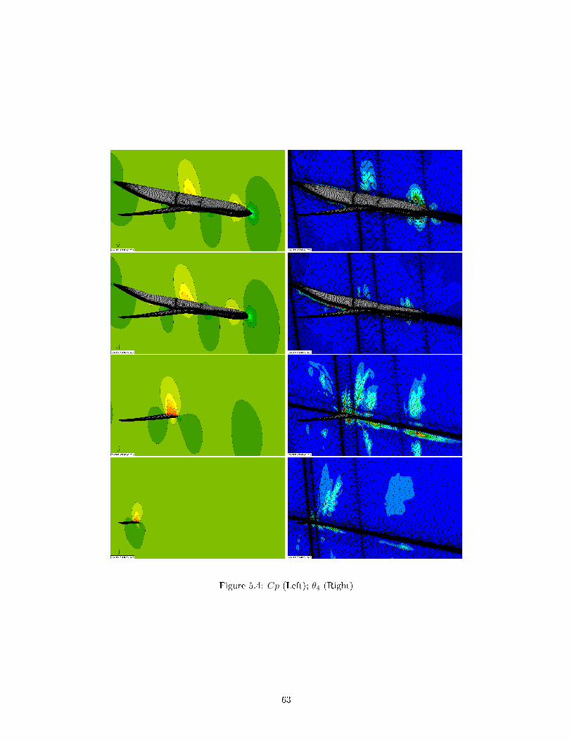
Figure 5.4: Cp (Left); θ4 (Right)

63

5.4 Conclusions

After the mathematical construction of the dierent steps involved in the adaptation process,a study of the dierent steps has been performed. The strategy used to adapt the grids for thecalculation of the function has been proved in the previous chapters (for a test case 2D) to beecient and beside the approximations made, the local sensors has allowed the individuationof the zones with an high sensitivity with respect to the functions chosen. The grid adaptationinduced has allowed the improvement on the function estimation accuracy and the global sensorbuilt has been shown to indicate when a mesh is more or less adapted for the calculation of thefunctional chosen. With this chapter an extension to an industrial case 3D of the sensor allowedits the validation for an industrial case in which the computational cost is more important, thephysic is more complex and the geometry (i.e multi blocks and non coincident grids) is moresophisticated.

64

Conclusions

The goal of this study was to build a strategy in order to answer to the need of accuracy on theevaluation of aerodynamic performances (i.e lift and drag) which are closely connected with thefuel consumption. Furthermore it was required to build a strategy which allows this improvementwithout to increase the computational cost of the CFD solution, leading to a redistribution ofpoints rather than an addition. The construction of such a method has been performed startingby theoretical considerations on the stability of a mesh which are described at the beginning ofthe second chapter. In the following of the chapter we described step by step the theoreticalaspects leading to the denition of a sensor θi,j used to induce the adaptation, and anothersensor or criterion θ used to qualify the mesh. The study and the coherence of these sensorsw.r.t our purposes is presented within the chapter three. In this chapter it was concluded thatthe sensor and the criterion are able to be used for our scopes. Then a mesh adaptation processwas exhibited within the fourth chapter in order to achieve an improvement of the accuracy.Here we chose Cd and Clp as goal functions and we compared the estimation of these variablesfor adapted meshes with respect to limiting values obtained from a calculation of Cd and Clp ona very ne mesh and we proved the increasing of the goals estimation accuracy. In chapter fourthwe also performed a comparison between our method and the gradient based one, showing thebenets of our strategy. Then an extension in a 3D industrial case of the is performed showinghis reliability in complex cases. This extension has been showed up in chapter ve where wealso retained to point out from a practical point of view that the sensor is enough mature to beused for an industrial application (i.e A320neo A380 and A350).

Beside we manage with some limits, the present work showed that the total derivative ofan aerodynamic function with respect to the volume mesh can be successfully used to builda strategy to adapt the mesh. Furthermore the strategy built from dF/dX presents otheradditional aspect of improvement. The νT = const and the thin boundary layer hypothesis madewithin the linearization of the term ∂R/∂W cause a deterioration of the accuracy of dF/dX.The limit constituted by these hypothesis can be removed in the future in order to enhance animprovement of θi,j . The geometric limit constituted by the xed points can be eliminated inorder to obtain a points redistribution totally coherent with the zones individuated by θi,j .

66

Appendix A

Construction of a mesh generation

elliptic system of PDEs

The generation of a structured mesh is following. We dene a computational space C as a unitsquare with coordinates ξξξ, a parameter space as unite square P with coordinates sss and thephysical domain D with physic coordinates xxx.

The mesh used for CFD is here dened as a map which associates every element of thecomputational space to the elements of the physical domain. Furthermore we dene it as:

xxx: C → D,

such that every single node on the physical space is the map of a node in the computationaldomain. The construction of the map C → D can be written as the combination of the mapsC → P and P → D.

In practice C → P and D → P are rst computed. In fact this last one is imposed asharmonic function:

∆sss =

3∑k=1

∂2sss

∂x2k

= 0. (A.1)

After the setting of the map D → P , and after the observation that the solution of theseequations depend on the boundary conditions, the only variable is the choice of the map C →P .

We dene now certain quantities which will be useful in the following:

gigigi = ∂xxx∂ξi

covariant base vectors

gigigi = ∂ξ∂xixixi

contravariant base vectors

Aij = gij = (gi, gjgi, gjgi, gj) covariant metric tensorBij = gij = (gi, gjgi, gjgi, gj) cotravariant metric tensor

Where the covariant and contra-variant metric tensor are linked by:

B = A−1

Observing that the vector sss can be expressed in respect to both the variables xxx and ξξξ as:

sss(xxx) = sss(ξξξ(xxx))

his Laplacian assumes the form:

∆sss =

3∑i,j=1

gijsssξiξj +

3∑k=1

∆ξksssξk . (A.2)

68

Now we impose the condition of regularity (∆sss = 0) and we observe that the last equationcan be expressed as:

∆ξξξ =

3∑i,j=1

gijPij . (A.3)

If we recall the equation in variable sss and we substitute the variable xxx we can write it downas:

∆xxx =

3∑i,j=1

gijxxxξiξj +

3∑k=1

∆ξkxxxξk . (A.4)

Now we observe that ∆xxx = 0 and we substitute the expression in ∆ξξξ to obtain:

3∑i,j=1

gijxξiξj +

3∑k=1

3∑i,j=1

gijPk

ijxξk = 0. (A.5)

with control functions:

Pk =

3∑i,j=1

gij

gkkPk

ij . (A.6)

In order to conclude we observe that this expression is written in the form which can be usedto solve the problem because it directly linked with the discretization being the covariant andcontra-variant variables expressible as nite dierences as we wrote down in the article.

69

Bibliography

[1] L Cambier and JP Veuillot. Status of the elsa cfd software for ow simulation and multi-disciplinary applications. AIAA paper, 2008.

[2] Richard P Dwight. Heuristic a posteriori estimation of error due to dissipation in nitevolume schemes and application to mesh adaptation. Journal of Computational Physics,2008.

[3] A Jameson, W Schmidt, and E Turkel. Numerical solution of the euler equations by nitevolume method using rungekutta time stepping schemes. AIAA Paper.

[4] R. Sauvage M. Meaux J.A. Desideri M. Nguyen-Dinh, J. Peter. Mesh qualication and

local adaptation based on total derivatives of aerodynamic functions w.r.t. mesh coordinates.

Application to Eulerian ow computation. 2012.

[5] Eric J Nielsen and Michael A Park. Using an adjoint approach to eliminate mesh sensitivitiesin computational design. AIAA journal, 2006.

[6] Jacques Peter. Introduction à l'optimisation de forme en aérodynamique et quelques ex-emples d'application. Oce national d'études et de recherches aerospatiales, 2006.

[7] Jacques Peter, Maxime Nguyen-Dinh, and Pierre Trontin. Goal oriented mesh adaptationusing total derivative of aerodynamic functions with respect to mesh coordinates. withapplications to euler ows. Computers & uids, 2012.

[8] Jacques EV Peter and Richard P Dwight. Numerical sensitivity analysis for aerodynamicoptimization: A survey of approaches. Computers & Fluids, 2010.

[9] Philip L Roe. Approximate riemann solvers, parameter vectors, and dierence schemes.Journal of computational physics, 1981.

[10] Bharat K Soni, Roy Koomullil, David S Thompson, and Hugh Thornburg. Solution adaptivegrid strategies based on point redistribution. Computer Methods in Applied Mechanics and

Engineering, 2000.

[11] Allmaras Spalart. A one equation turbulence model for aerodinamic ows. AIAA journal.

[12] Stephanus Petrus Spekreijse. Elliptic grid generation based on laplace equations and alge-braic transformations. Journal of Computational Physics, 1995.

[13] GD Van Albada, B Van Leer, and WW Roberts Jr. A comparative study of computational

methods in cosmic gas dynamics. 1997.

[14] Bram Van Leer. Towards the ultimate conservative dierence scheme. v. a second-ordersequel to godunov's method. Journal of computational Physics, 1979.

[15] David A Venditti and David L Darmofal. Anisotropic grid adaptation for functional outputs:application to two-dimensional viscous ows. Journal of Computational Physics, 2003.

70