POLITECNICO DI MILANO · 2013-03-05 · POLITECNICO DI MILANO POLO REGIONALE DI COMO Master of Science in Management, Economics and Industrial Engineering Strategic Distribution Network

POLITECNICO DI MILANO

POLO REGIONALE DI COMO

Master of Science in

Management, Economics and Industrial Engineering

Strategic Distribution Network Design:

Quantitative tuning of the distribution network

selection matrixes

Supervisor:

Co-supervisor

:

Alessandro PEREGO

Riccardo MANGIARACINA

Master graduate thesis by:

Andrii ZELENKO

Guang SONG

Id number: 754438

Id number: 749644

Academic Year 2011/2012

1

INDEX

Executive Summary .......................................................................................................................... 12

Reason to start the research ...................................................................................................... 12

Objective ................................................................................................................................... 12

Methodology ............................................................................................................................. 14

Results ....................................................................................................................................... 16

Consumer Electronics Industry......................................................................................... 16

FMCG Industry ................................................................................................................. 20

Chapter 1. Literature Review: Methodologies to support designing-redesigning of the distribution

network .............................................................................................................................................. 24

1.1 Introduction ......................................................................................................................... 24

1.2 The definition and main methods for the design of the distribution network presented in

the literature .............................................................................................................................. 25

1.2.1 Distribution network design definition and key factors influence the designing

process ............................................................................................................................... 25

1.2.2 Methodology for planning the logistics strategy ..................................................... 27

1.2.3 Methodology “Integrated Planning Support Framework” ...................................... 32

1.2.4 Ballou‟s methodology .............................................................................................. 37

1.2.5 Distribution network selection matrix ..................................................................... 45

1.3 Mathematical methodologies coupling the selection process ............................................ 46

1.3.1 Mathematical methodologies coupling the selection process ................................. 46

Chapter 2. The Selection of Drivers ................................................................................................. 49

2.1 Definition of the drivers ...................................................................................................... 49

2.2 Measurement method of the drivers ................................................................................... 61

Chapter 3. The Case Studies ............................................................................................................. 69

3.1 Data collection of Consumer Electronics Industry ............................................................. 69

3.1.1 Hewlett Packard ....................................................................................................... 69

3.1.2 Sony ......................................................................................................................... 70

3.1.3 Samsung ................................................................................................................... 73

2

3.2 Data collection of FMCG Industry ..................................................................................... 76

3.2.1 Nestle Italia .............................................................................................................. 76

3.2.2 Calzedonia................................................................................................................ 78

3.2.3 Reckitt Benckiser ..................................................................................................... 79

3.2.4 Coca-Cola Italia ....................................................................................................... 80

3.2.5 3M ............................................................................................................................ 81

3.2.6 Unilever Bestfoods .................................................................................................. 83

3.2.7 Hackman .................................................................................................................. 84

Chapter 4. The Description of Mathematical Methodology ............................................................. 86

4.1 The main procedure of mathematical analysis ................................................................... 86

4.2 The description of mathematical tools ................................................................................ 88

4.2.1 Descriptive statistics ................................................................................................ 88

4.2.2 Correlation analysis ................................................................................................. 89

4.2.3 Confirmatory factor analysis ................................................................................... 90

4.2.4 Principal component regression............................................................................... 92

Chapter 5. Application of the Mathematical Models........................................................................ 94

5.1 Application in Consumer Electronics Industry................................................................... 94

5.1.1 Descriptive statistics analysis .................................................................................. 94

5.1.2 Correlation analysis ................................................................................................. 97

5.1.3 Confirmatory factor analysis ................................................................................. 105

5.1.4 Principal component regression............................................................................. 119

5.2 Application in FMCG Industry ......................................................................................... 121

5.2.1 Descriptive statistics .............................................................................................. 121

5.2.2 Correlation analysis ............................................................................................... 123

5.2.3 Confirmatory factor analysis ................................................................................. 128

5.2.4 Principal component regression............................................................................. 141

Chapter 6. Results ........................................................................................................................... 143

6.1 Result of Consumer Electronics Industry ......................................................................... 143

6.1.1 Analysis of four basic characteristics of distribution problem .............................. 143

3

6.1.2 Analysis of Firm and Market characteristics ......................................................... 144

6.1.3 Relationship between distribution problem and distribution solution .................. 145

6.2 Result of FMCG Industry ................................................................................................. 147

6.2.1 Analysis of four basic characteristics of distribution problem .............................. 147

6.2.2 Analysis of Firm and Market characteristics ......................................................... 148

6.2.3 Relationship between distribution problem and distribution solution .................. 150

Chapter 7. Conclusion ..................................................................................................................... 152

7.1 Comparison of drivers in different industries ................................................................... 152

7.2 Comparison of drivers‟ coefficients and regression functions ......................................... 154

7.3 Comparison of normative selection matrixes ................................................................... 155

7.4 Further development ......................................................................................................... 157

Bibliography: .................................................................................................................................. 158

Appendix ......................................................................................................................................... 162

Criticality value for Consumer Electronic industry................................................................ 162

Criticality value for FMCG industry ...................................................................................... 166

4

INDEX of Figures

Figure 1 Research procedure．．．．．．．．．．．．．．．．．．．．．．．．．．．．．．．．．．．．．．．．．．．．．．．．．．．．．．13

Figure 2 Flow chart of Ballou‟s methodology．．．．．．．．．．．．．．．．．．．．．．．．．．．．．．．．．．．．．．．．37

Figure 3 Theoretic model of distribution network selection matrix．．．．．．．．．．．．．．．．．．．．．．．．44

Figure 4 The procedure of mathematical analysis．．．．．．．．．．．．．．．．．．．．．．．．．．．．．．．．．．．．．85

5

INDEX of Graphs

Graph 1 Theoretical model of CFA in Consumer Electronics industry．．．．．．．．．．．．．．．．．．．．105

Graph 2 Theoretical model of CFA in FMCG industry．．．．．．．．．．．．．．．．．．．．．．．．．．．．．．．．127

Graph 3 Scatter diagram of distribution problems in Consumer Electronics industry．．．．．．．．．145

Graph 4 Relationship diagram in Consumer Electronics industry．．．．．．．．．．．．．．．．．．．．．．．．146

Graph 5 Scatter diagram of distribution problems in FMCG industry．．．．．．．．．．．．．．．．．．．．．149

Graph 6 Relationship diagram in FMCG industry．．．．．．．．．．．．．．．．．．．．．．．．．．．．．．．．．．．．150

Graph 7 Normative matrix in Consumer Electronics industry．．．．．．．．．．．．．．．．．．．．．．．．．．．155

Graph 8 Normative matrix in FMCG industry．．．．．．．．．．．．．．．．．．．．．．．．．．．．．．．．．．．．．．．155

6

INDEX of Tables

Table 1 Driver list in Consumer Electronics Industry．．．．．．．．．．．．．．．．．．．．．．．．．．．．．．．．．．．16

Table 2 Regression coefficient in Consumer Electronics industry．．．．．．．．．．．．．．．．．．．．．．．．．17

Table 3 Driver list in FMCG Industry．．．．．．．．．．．．．．．．．．．．．．．．．．．．．．．．．．．．．．．．．．．．．．．20

Table 4 Regression coefficient in FMCG industry．．．．．．．．．．．．．．．．．．．．．．．．．．．．．．．．．．．．．21

Table 5 Measurement criterion on stage of life cycle．．．．．．．．．．．．．．．．．．．．．．．．．．．．．．．．．．．61

Table 6 Measurement criterion on handling characteristic．．．．．．．．．．．．．．．．．．．．．．．．．．．．．．．62

Table 7 Original value of drivers in HP．．．．．．．．．．．．．．．．．．．．．．．．．．．．．．．．．．．．．．．．．．．．．69

Table 8 Original value of drivers in Sony．．．．．．．．．．．．．．．．．．．．．．．．．．．．．．．．．．．．．．．．．．．．71

Table 9 Original value of drivers in Samsung．．．．．．．．．．．．．．．．．．．．．．．．．．．．．．．．．．．．．．．．．75

Table 10 Original value of drivers in Nestle．．．．．．．．．．．．．．．．．．．．．．．．．．．．．．．．．．．．．．．．．．77

Table 11 Original value of drivers in Calzedonia．．．．．．．．．．．．．．．．．．．．．．．．．．．．．．．．．．．．．．78

Table 12 Original value of drivers in Reckitt Benckiser．．．．．．．．．．．．．．．．．．．．．．．．．．．．．．．．．79

Table 13 Original value of drivers in Coca-Cola．．．．．．．．．．．．．．．．．．．．．．．．．．．．．．．．．．．．．．80

Table 14 Original value of drivers in 3M．．．．．．．．．．．．．．．．．．．．．．．．．．．．．．．．．．．．．．．．．．．．82

Table 15 Original value of drivers in Unilever Bestfoods．．．．．．．．．．．．．．．．．．．．．．．．．．．．．．．83

Table 16 Original value of drivers in Hackman．．．．．．．．．．．．．．．．．．．．．．．．．．．．．．．．．．．．．．．84

Table 17 Descriptive statistics result 1 in Consumer Electronics industry．．．．．．．．．．．．．．．．．．．94




Table 21 Correlation analysis result 1 in Consumer Electronics industry．．．．．．．．．．．．．．．．．．．97

7

Table 22 Correlation analysis result 2 in Consumer Electronics industry．．．．．．．．．．．．．．．．．．．99

Table 23 Correlation analysis result 3 in Consumer Electronics industry．．．．．．．．．．．．．．．．．．101

Table 24 Correlation analysis result 4 in Consumer Electronics industry．．．．．．．．．．．．．．．．．．102

Table 25 Driver list after correlation analysis in Consumer Electronics industry．．．．．．．．．．．．103

Table 26 Recommended value of goodness-of-fit for CFA．．．．．．．．．．．．．．．．．．．．．．．．．．．．．105

Table 27 Hypotheses for CFA in Consumer Electronics industry．．．．．．．．．．．．．．．．．．．．．．．．．110

Table 28 Initial result of CFA for product factor in Consumer Electronics industry．．．．．．．．．．111

Table 29 Final result of CFA for product factor in Consumer Electronics industry．．．．．．．．．．．112

Table 30 Initial result of CFA for service factor in Consumer Electronics industry．．．．．．．．．．．113

Table 31 Final result of CFA for service factor in Consumer Electronics industry．．．．．．．．．．．113

Table 32 Initial result of CFA for demand factor in Consumer Electronics industry．．．．．．．．．．114

Table 33 Final result of CFA for demand factor in Consumer Electronics industry．．．．．．．．．．．115

Table 34 Final result of CFA for supply factor in Consumer Electronics industry．．．．．．．．．．．．115

Table 35 Driver list after CFA in Consumer Electronics industry．．．．．．．．．．．．．．．．．．．．．．．．116

Table 36 Hypotheses result of CFA in Consumer Electronics industry．．．．．．．．．．．．．．．．．．．．118

Table 37 Distribution solution in Consumer Electronics industry．．．．．．．．．．．．．．．．．．．．．．．．118

Table 38 Regression coefficient of drivers in Consumer Electronics industry．．．．．．．．．．．．．．．120

Table 39 Descriptive statistics result 1 in FMCG industry．．．．．．．．．．．．．．．．．．．．．．．．．．．．．．121




Table 43 Correlation analysis result 1 in FMCG industry．．．．．．．．．．．．．．．．．．．．．．．．．．．．．．122

8




Table 47 Driver list after correlation analysis in FMCG industry．．．．．．．．．．．．．．．．．．．．．．．．126

Table 48 Hypotheses for CFA in FMCG industry．．．．．．．．．．．．．．．．．．．．．．．．．．．．．．．．．．．．．132

Table 49 Initial result of CFA for product factor in FMCG industry．．．．．．．．．．．．．．．．．．．．．．133

Table 50 Final result of CFA for product factor in FMCG industry．．．．．．．．．．．．．．．．．．．．．．．134

Table 51 Initial result of CFA for service factor in FMCG industry．．．．．．．．．．．．．．．．．．．．．．．135

Table 52 Final result of CFA for service factor in FMCG industry．．．．．．．．．．．．．．．．．．．．．．．135

Table 53 Initial result of CFA for demand factor in FMCG industry．．．．．．．．．．．．．．．．．．．．．．136

Table 54 Final result of CFA for demand factor in FMCG industry．．．．．．．．．．．．．．．．．．．．．．．137

Table 55 Final result of CFA for supply factor in FMCG industry．．．．．．．．．．．．．．．．．．．．．．．．137

Table 56 Driver list after CFA in FMCG industry．．．．．．．．．．．．．．．．．．．．．．．．．．．．．．．．．．．．138

Table 57 Hypotheses result of CFA in FMCG industry．．．．．．．．．．．．．．．．．．．．．．．．．．．．．．．．139

Table 58 Distribution solution in FMCG industry．．．．．．．．．．．．．．．．．．．．．．．．．．．．．．．．．．．．140

Table 59 Regression coefficient of drivers in FMCG industry．．．．．．．．．．．．．．．．．．．．．．．．．．．141

Table 60 Values of basic characteristics in Consumer Electronics industry．．．．．．．．．．．．．．．．．143

Table 61 Result of Firm and Market characteristics in Consumer Electronics industry．．．．．．．．144

Table 62 Values of basic characteristics in FMCG industry．．．．．．．．．．．．．．．．．．．．．．．．．．．．．147

Table 63 Result of Firm and Market characteristics in FNCG industry．．．．．．．．．．．．．．．．．．．．148

Table 64 Result transformation in FMCG industry．．．．．．．．．．．．．．．．．．．．．．．．．．．．．．．．．．．．149

Table 65 Comparison of drivers．．．．．．．．．．．．．．．．．．．．．．．．．．．．．．．．．．．．．．．．．．．．．．．．．．152

9

Table 66 Comparison of drivers‟ coefficients．．．．．．．．．．．．．．．．．．．．．．．．．．．．．．．．．．．．．．．．154

Table 67 Result of goodness-of-fit for PCR．．．．．．．．．．．．．．．．．．．．．．．．．．．．．．．．．．．．．．．．．154

10

Abstract

The thesis is devoted to define the way of optimizing and tuning the existing

distribution network model using quantitative mathematical methodologies.

In this work considered the mathematical approach to describe the process of

tuning distribution network selection matrixes based on several quantitative

methodologies that describe the relationship between distribution problem and

distribution solution. The given approach can support the distribution network

designers in strategic decision-making process about the future configuration of the

distribution network, which is based on the match between distribution problem

reflecting the products, service, demand and supply characteristics presented by firm,

and distribution solution indicating the level of decentralization of the distribution

network.

Key words: DISTRIBUTION NETWORK DESIGN, SELECTION MATRIXES,

CORRELATION, CONFIRMATORY FACTOR ANALYSIS, DRIVERS‟ POOL,

ARCS, NODES, ELECTRONICS INDUSTRY, FMCG.

11

In questo lavoro di tesi è stato definito il modo di ottimizzare e mettere a punto

l‟attuale modello di rete di distribuzione utillizando metodologie matematiche.

E‟ stato considerato il metodo matematico per descrivere il processo di messa a

punto di matrici selettive della rete distributiva basata su diverse metodologie

quantitative che descrivono la relazione tra problemi di distribuzione e la soluzione di

distribuzione. L‟approccio dato è in grado di supportare i progettisti nel prendere

decisioni strategiche circa la futura configurazione della rete di distribuzione, che si

basa sulla corrispondenza tra problemi di distribuzione, che riflettono i prodotti, i

servizi, le caratteristiche della domanda e dell‟offerta presentata dalla società, e tra la

soluzione di distribuzione, indicante il livello di decentramento della rete di

distribuzione.

Parole chiave: PROGETTAZIONE DI UNA RETE DI DISTRIBUZIONE, MATRICI

SELETTIVE, CORRELAZIONE, ANALISI FATTORIALE CONFERMATIVA,

DRIVERS‟ POOL, NODI, INDUSTRIA ELETTRONICA, FMCG.

12

Executive Summary

Reason to start the research

The distribution network design model consists of a wide range of issues

involving the strategic decisions, tactical decisions and operational decisions in

logistics management. The strategic planning attempts to design a rough structure of

distribution network. Tactical level decisions refer to the exact position of the facility,

the selection of the transportation, level of the inventory and so on. The operational

planning aims at coping with the routine decisions of distribution process.

In this study, we need to optimize the existing distribution network selection

matrix, which can solve the problems on strategic level of the distribution process.

This network selection matrix is a kind of decision making tool used to determine the

number of echelons, number of facilities in each echelon, and type of facility in the

distribution network.

The existing distribution network selection matrix has been built based mainly on

the qualitative way, despite a few of quantitative approaches were used to develop the

matrix. The purpose of this study is trying to make the matrix more accurate by using

mathematical models purely in order to avoid the subjectivity and bias of qualitative

approach.

Objective

This thesis aims at optimizing the existing distribution network selection matrixes

in Consumer Electronics industries and Fast Moving Consumer Goods industry

(FMCG) in European level by taking mathematical method to find a more accurate

relationship between distribution problem and distribution solution.

13

For the purpose of this main goal, we must achieve the following sub-objectives:

- Collecting drivers used to design distribution network for the sake of making the

existing driver list to be completed;

- Identifying the mathematical models in order to obtain the more important drivers,

which are more able to reflect the distribution problem based on the nature of

industry;

- Filtering the drivers based on the application of mathematical tools;

- Figuring out the coefficient of each driver and evaluation function by using

regression analysis after the driver selection;

- Finding out the accurate relationship between distribution problem and

distribution solution based on the result of preceding sub-objective;

- Achieving the normative distribution network selection matrixes in Consumer

Electronics industry and FMCG industry.

The distribution network selection matrix can support the users to make the

strategic decisions on the configuration of distribution network, which is based on the

match between distribution problem reflecting the products, service, demand and

supply characteristics presented by firm, and distribution solution indicating the

decentralization of the distribution network. Thereby, the correct distribution network

could be obtained if the relationship between distribution problem and distribution

solution can be described in an accurate way.

The existing model is able to describe the relationship between distribution

problem and distribution solution. However, we assume that this relationship could be

stronger because the mathematical tools should allow a more objective selection of

the drives and a more accurate determination of the driver‟s coefficient in affecting

the distribution network structure. Therefore, the core of this study is to refine the

distribution network selection matrix by quantitative method in order to avoid the

subjectivity and bias of qualitative approach and improve reliability.

14

Methodology

In order to achieve the objectives mentioned above, there are five main processes

and seven micro steps we have to implement. The whole procedure is shown as the

following figure:

Figure 1 Research procedure

Firstly, we try to find more drivers in order to updating the current driver list. In

the existing distribution network selection matrix, there are 22 drivers divided into

Collecting drivers by literature study

Evaluating the original value of drivers and

ranking them to five-points scale

Descriptive statistics analysis

Correlation analysis

Confirmatory factor analysis

Regression analysis

Representing the distribution problem and

distribution solution by graphic illustration

Enlarging

driver list

Estimating

the drivers

Filtering the

drivers

Figuring out the

drivers’ weights

and evaluation

function

Obtaining the

normative

matrixes

15

four groups (product, service, demand, and supply). We have to collect more drivers,

which are not included in the current driver list, in order to make the driver list to be

more completed.

Secondly, we need to evaluate the punctual value of drivers, and rank them based

on the five-point scale for the subsequently data analysis. In this study, we don‟t

interview the firms directly because of the time constraint. With regard to the existing

drivers, we can find their value from historic data collected by previous research.

Taking advantage of the annual report and company‟s official website, the value of

new drivers could be found.

After this, we have achieved a lot of drivers. We suppose that the distribution

problems in one industry area can be described by part of these drivers we collected.

Therefore, the following steps are to carry out the data analysis in order to filter the

drivers. We intend to find out the more important drivers could depict the distribution

problem based on the nature of an industry. We use descriptive statistics analysis and

correlation analysis to see if some drivers could be removed or combined according to

their standard deviation and correlation factor. The further analysis will be done by

confirmatory factor analysis (CFA). The CFA model can reduce more drivers on the

basis of the current theoretical model of distribution network selection matrix and the

correlation matrix of the drivers.

According to the preceding process, we can obtain some more important drivers.

The following step is to figure out the regression function for those important drivers

and their regression coefficients. By taking into consideration the multicollinearity

may exist among the drivers, we have to use principal component regression (PCR)

model to solve this problem.

In the last step, we use the regression function and regression coefficients of the

drivers to figure out the factors of Firm and Market characteristics for every

distribution problem, and represent their value on the two-dimension graph to

discover the relationship between distribution problem and distribution solution. The

16

value of Firm characteristic is the sum of the driver‟s factor in product and supply

characteristics, and the value of Market characteristics is the sum of the driver‟s factor

in service and demand characteristics.

Results

Consumer Electronics Industry

Available drivers after quantitative analyses

After the descriptive statistics analysis, correlation analysis and confirmatory

factor analysis, we get 20 available drivers for Consumer Electronics industry. Some

drivers are deleted and/or combined due to the meaningless standard deviation factor,

the high correlation factor and low factor loading.

Product

Variety

Product value density

Contribution margin

Product complexity

Stage of life cycle

ABC product characteristic

Level of competition

Service

Cycle time

Completeness

Accuracy & Punctuality

Customer experience

Demand

Dimension of the orders

Delivery frequency

Predictability of demand

Demand volatility

Demand level

17

Supply

Number of plants

Distance from plant to client

Level of specialization

Exclusivity of production in a plant

Table 1 Driver list in Consumer Electronics Industry

Regression function and coefficients

The regression function and relative drivers‟ coefficients are obtained by using

the principal component regression analysis on SPSS. The value of adjusted R2 and F

estimator shows a well goodness-of-fit.

solution=-5.8029+(0.1748)variety+(-0.116)pvd+(-0.116)conmarg+(0.3773)procomp+(0.231)stalc

+(0.6049)abcchar+(0.6049)levcomp+(-0.7206)cyctime+(2.5535)complet+(-0.2756)accupun+(-0.0

163)cusexpe+(0.6176)dimorde+(0.0882)delfreq+(0.3024)preddem+(-0.6049)demdvol+(-0.1906)d

emdlev+(0.0776)numplat+(0.1388)distptc+(-0.3341)levlspe+(-0.0795)exclpro

R2=0.952, adjusted R

2=0.856, F (10,5) =9.884, P=0.010

Consumer Electronics Industry Regression coefficient

Constant 5.8029

Variety 0.1748

Physical Value Density -0.1160

Contribution Margin -0.1160

Product Complexity 0.3773

Stage of Life Cycle 0.2310

ABC product characteristic 0.6049

Level of Competition 0.6049

Cycle Time -0.7206

Completeness 2.5535

Accuracy & Punctuality -0.2756

Customer Experience -0.0163

Dimension of the order 0.6176

Delivery Frequency 0.0882

18

Predictability of Demand 0.3024

Demand Volatility -0.6049

Demand Level -0.1906

Number of Plants 0.0776

Distance from plant to client 0.1388

Level of Specialization -0.3341

Exclusivity of production in a plant -0.0795

Table 2 Regression coefficient in Consumer Electronics industry

Relationship between distribution problem and distribution solution

We figure out the value of Firm and Market characteristics of every distribution

problem and plot down the values we got on the chart (shown below). Each

distribution problem is marked with its own spot on the chart, has the name and the

value of distribution solution. For instance, SA1,1 means that we consider distribution

problem Samsung1 (SA1) and distribution solution for this problem is 1 (direct

shipment).

The value of the distribution solution is already scaled and the meaning of the

scale is given below:

1: direct shipment;

19

2: 1 echelon with a few Warehouses/Transit Points (up to 3);

3: 2 echelons with a few Warehouses/Transit Points (up to 5) in the 1st

echelon and a few Warehouses/Transit Points (less than 15) in the 2nd

echelon;

4: 2 echelons with a few Warehouses/Transit points (up to 5) in the 1st

echelon and several Warehouses/Transit Points (15 – 20) in the 2nd

echelon;


echelon and many Warehouses/Transit Points (more than 20) in the 2nd

echelon;

We use colored line to highlight the border of different distribution solution area

on the chart thus we can achieve a clear illustration about the feature of distribution

problem and the decentralization of distribution solution. The red, yellow and green

line indicates the direct shipment, one level network and two levels network

respectively.

Removing the plot of each distribution problem from the above diagram, we can

achieve a clear normative distribution network selection matrix in Consumer

Electronics industry. We can see that the distribution solution turns to be more

decentralized in case the values of Firm and Market characteristics increase.

◆Direct shipment

◆1 level

◆2 levels (1CW+TPs)


━ Direct shipment border

━ 1 level border

━2 levels (1CW+TPs) border

20

FMCG Industry

Available drivers after quantitative analyses

Based on the same research procedure and methodology, we obtain 17 available

drivers for FMCG industry.

Product

Variety


Risk of obsolescence

Product complexity


Production strategy

Service

Completeness

Accuracy

Customer experience

Punctuality

Demand


Number of customers

Delivery frequency

2 levels

CWs (≤5)

+TPs (<15)

Direct shipment

1 level network with CWs

(≤3)

2 levels network with CW (≤5) + TPs (≥15)

21

Predictability

Supply

Number of plants



Table 3 Driver list in FMCG Industry

Regression function and coefficients

The regression function and coefficients are shown below. The results of adjusted

R2 and F estimator demonstrate the model‟s fit is good as well.

solutio=-14.0376+(-0.3636)variety+(-0.4481)pvd+(0.5065)riskobs+(0.218)complex+(-0.0971)compet+

(1.0615)prodstr+(1.2107)complet+(0.3362)accur+(1.9791)cusexpe+(-0.2913)punct+(-0.3766)dimord+(

0.1883)numcus+(0.0715)delfreq+(0.9039)predict+(-0.0919)numplan+(-0.0781)distptc+(-0.3961)exclu


2=0.990, F (11,1) =107.394, P=0.075

FMCG Industry Regression coefficient

Constant -14.0376

Variety -0.3636


Risk of Obsolescence 0.5065


Level of Competition -0.0971

Product Strategy 1.0615

Completeness 1.2107

Accuracy 0.3362

Customer Experience 1.9791

Punctuality -0.2913

Dimension of the Order -03766

Number of Customers 0.1883



Number of Plants -0.0919

22

Distance from plant to client -0.0781


Table 4 Regression coefficient in FMCG industry

Relationship between distribution problem and distribution solution

Like the Consumer Electronics industry case, we plot down the values of Firm

and Market characteristics on the chart (shown below). Each distribution problem is

marked with its own spot on the chart, has the name and the value of distribution

solution. For instance, Nestle3,5 means that we consider distribution problem Nestle3

and distribution solution for this problem is 5 (two echelons with several WH/TP in

the first echelon and many WH/TP in the second one).

Each distribution solution is marked with color that illustrates their belonging to

one of the four groups (the chart is given below):

In the group marked with yellow we have distribution solutions characterized

by having just one level in the distribution network;

In the group marked with green color we have distribution solutions

characterized by having two levels in the distribution network with less than 5

Warehouses in the 1st echelons and number of Transit Points in the 2

nd one

23

In the group marked with blue color we have 2 levels distribution solutions

with more than 5 Warehouses in the 1st echelon and number of Transit Points

in the second one.

We can highlight the areas with the high concentration of the spots belonging to

the particular group. The chart with the areas is presented below.

We take the same operation as the Consumer Electronics industry. The normative

matrix of FMCG industry can be generated as shown below. The distribution solution

becomes more decentralized if the values of Firm and Market increase.

1 level network with CWs or TPs

2 levels network with CWs (≤3) + TPs

2 levels network with CWs (>3) + TPs

24

Chapter 1. Literature Review: Methodologies to support

designing-redesigning of the distribution network

1.1 Introduction

In this section we want to present some methodologies proposed by different

authors related to the distribution network design problem. These methodologies

provide a systematic approach to the problem of configuration (or reconfiguration) of

the distribution network, splitting the decision-making process into steps, more

manageable, which support is often provided using of operational research models

and specific applications. In addition, for better understanding of the methodologies

presented, we will provide some real examples.

The literature analysis has shown that the methodologies helping to solve

distribution network design problem can be grouped into two main

categories/classes. The first class is represented by so-called “complete design”

methods that address the entire design problem: strategic choices (network design,

transport modes, etc.), operational choices (policies to manage the flow of materials,

local delivery of programs, etc.). The second group includes the “partial” methods

that are useful in solving some sub-problems related to the design of the distribution

network. In particular, these methods focus mainly on the question of location -

allocation of facilities, or on the issue concerning the location of nodes.

It was decided to describe only the main methods belonging to the first group, as

providing procedures to support the entire design problem, due to the fact that these

methods are more interesting for the purposes of this research work.

After the review of the main methodologies presented in the literature, the

proposal to support the decision about the design of the distribution network will be

highlighted.

25

1.2 The definition and main methods for the design of the

distribution network presented in the literature

1.2.1 Distribution network design definition and key factors influence the

designing process

Distribution network design problems involve strategic decisions which influence

tactical and operational decisions. Thereby, they are core problems for each company

(Ambrosino and Scutella, 2005) and are considered an important strategic weapon to

achieve and maintain competitive strength (Mourtis and Evers, 1995).

Distribution refers to the steps taken to move and store a product from the supplier

stage to a customer stage in the supply chain. Distribution is a key driver of the

overall profitability of a firm because it directly impacts both the supply chain cost

and the customer experience. Good distribution can be used to achieve a variety of

supply chain objectives ranging from low cost to high responsiveness (Sunil Chopra,

2003).

As an essential part of the entire supply chain, distribution process comprises

several decision issues. According to the previous contributions, the distribution

system design revolves around three key decision areas of: inventory policy, facility

location, and transport selection routing (Ronald H. Ballou, 1993). Hence, the relevant

cost elements have to be distinguished. The distribution network design affects the

following costs: inventories, transportation, facilities and handling, information (Sunil

Chopra,2003). Additionally, the relations between these cost components are soberly

logical: as the number of facilities in a supply chain increases, the inventory and

resulting inventory costs also increase. As long as inbound transportation economies

of scale are maintained, increasing the number of facilities decreases total

transportation cost. If the number of facilities is increased to a point where there is a

significant loss of economies of scale in inbound transportation, increasing the

number of facilities increase total transportation cost. Facility costs decrease as the

26

number of facilities is reduced, because a consolidation of facilities allows a firm to

exploit economies of scale.

In order to design an appropriate distribution network, the trade-off between cost

elements is a crucial task (Van de Ven, 1993). Based on the experiences, each cost

element is related to several variables, that is to say, the selection of variables

determine the appropriate distribution channels (Payne and Peters, 2004).

Ronald H. Ballou (1993) declares the product characteristics refer to the important

logistical characteristics. Regarding the product characteristics, Marshall Fisher (1997)

distinguished between functional and innovative products. He asserts that demand is

predictable, the product life cycle long, and the contribution margin thin for products

that are primarily functional; demand is unpredictable, the product life cycle short,

and the contribution margin more generous for products that are primarily innovative.

By taking into account the Fisher‟s theory, Christopher and Towill (2005) have

extended this approach to a five generic parameter classification; duration of life cycle,

time window, volume, variety and variability, known by the acronym DWV3. Besides,

more drivers associated the product characteristics, such as substitutability,

value/weight, weight/cubic volume ratio, competition, 80-20 principle, product

complexity and so on, have been mentioned by the current researchers in some

contributions (Lovell et al., 2005; Sharifi et al., 2006; Stavrulaki and Davis, 2010).

In addition to the product characteristics, there are some contributions

emphasized the importance of demand factor and service factor in the distribution

process. Sunil Chopra (2003) analyzes the effect of response time, order visibility and

returanability on the distribution network. Martin Christopher (2006) states that the

demand characteristics play a crucial role in selecting the logistics channel. Fari

Collin (2009) demonstrates that the task of logistics network design can be

approached from product drivers and customer (demand) drivers. Indeed, we can

found many drivers on the demand and service characteristics, for example, the

customer experience, number of customers, level of service, demand uncertainty,

27

forecasting accuracy, demand level, etc (Lovell et al., 2005; Sharifi et al., 2006;

Stavrulaki and Davis, 2010). What is more, from a border perspective, the drivers of

supplier‟s characteristics can determine the configuration of distribution network even

in the global scope (Archini and Banno, 2003; A. Creazza et al., 2010), for instance

the number of suppliers and supplier‟s location.

1.2.2 Methodology for planning the logistics strategy

The approach proposed by the authors Alan Rushton and Saw Richard

(2000) attracts particular interest, because this is a general criterion for the

problem formulation and evaluation of logistics strategy, planning that identifies

the distribution as integral part of the strategic planning process at corporate level. It

therefore develops a model that considers both business issues and logistics

issues, underlining the importance of identifying a distribution plan consistent

with the entire business strategy. The criterion presented has four sequential stages:

1. Analysis of the business environment.

2. Generation of possible logistics configurations.

3. Quantitative evaluation of alternatives generated.

4. Comparison with the company‟s business strategy.

Now let‟s have a look on them more in details.

1) Analysis of the business environment: the first step is the analysis of the

business environment within which the company operates in means the grouping of

all the factors to be considered in the design. These can be divided into:

External factors: hey are typically treated as exogenous and not depending on

the company. They may vary depending on the sector, of the particular company

and the market. Among the most important factors are:

o available types of transport;

28

o infrastructural changes;

o legislative changes;

o technological changes;

o development of information technologies (for instance, EDI);

o environmental impact;

o new trends in the sector (for example, considering the continuous

growth in the level of customer service, product life cycle shortening,

developing relationships with 3PL operators, the continuing trend to

reduce inventories in line with lean production policies);

Internal factors: these factors can be divided into qualitative factors and

quantitative factors. Both of these types of information are used to describe the

business in an operational context.

Typical examples of qualitative data: groups of products made by the company,

sources of supply, number and type of facilities, major transportation types used, used

material handling systems, cargo units, organizational, relationship with providers of

3PL , major customers, customer service performance, information systems available.

Regarding to the quantitative data are considered of the main flows of products,

depending on the division or the same type of transport, the demand by region and by

product, market segmentation, and service performance, analysis of the couriers,

profile of stocks, products and customers.

2) Generation of possible logistics configurations: the second phase of the

methodology is to generate several alternative configurations. It‟s very important to

give space to a large number of innovative solutions, because the planning horizon for

a distribution network is very wide: the decision maker must try to predict possible

future scenarios in order to create a system that can be sustainable. This could cause

difficulties for many companies: to overcome these obstacles it could be positive to

29

use external consultants and brainstorming techniques. These approaches allow you to

develop a long list of options, some of which may initially seem very feasible. Then

follows an analysis aimed at identifying what alternatives, including those proposed,

could be effectively adopted considering the planning horizon. The output of this

phase is then a short list of configurations to be analyzed in the next step, a

quantitative assessment.

3) Quantitative evaluation of alternatives generated: at this point starts the

third phase, which provides a quantitative assessment of the alternatives selected in

the previous one, using mathematical models: the limitation of these techniques is that

they do not allow to have an overall vision of the distribution network design

problem , but instead focus only on parts of the supply chain (location of warehouses,

vehicle routing, etc.), with the consequent risk of leading to suboptimal solutions. In

other words, there are no quantitative global optimization techniques, which

simultaneously consider all possible alternatives can be obtained by evaluating each

time the realization of potential products in all plants, the transfer of goods by all

modes of transportation available through all possible network

configurations. Furthermore, even if there were such a technique, the resulting

computational complexity makes it impractical to use.

This third phase of the problem considering the allocation of customers to sources

of production: one of the worst mistakes you can commit is to consider that the

minimum cost solution corresponds always to deliver the products required by each

market from the nearest facility, subject to the constraints of capacity. In some cases

this may be the optimal solution, however, when facilities have significant costs of

conversion (high set-up time) and different products can be manufactured with

different costs depending on the plant, maybe it could be more appropriate to supply

the markets production units geographically most distant, thereby supporting higher

transport costs, but lower production costs. Carefully considered all the main trade-off

between costs and then determined the allocation of customers to production sources,

it is necessary to evaluate in detail the modes to be adopted, the structure of the

30

network and the articulation of the stock through the distribution system. The most

common approach for this type of analysis involves the use of simulation techniques

and software developed for this purpose.

The most usual method is to simulate the operating costs for each possible

configuration. Several heuristic algorithms are also used as the criterion of the centre

of gravity, which suggest the optimal location of the deposits in order to reduce

transportation costs.

The method is based on the minimization of the transportation costs by finding the

centre of gravity:

i

iiiyx

yxdRFCostTotal )],([min)min(,

,

where:

),( yx – coordinates of the centre of gravity;

),( ii yx – coordinates of both the points of origin and destination;

iF – inbound (for the point of destination) and outbound (for the point of origin)

flows;

iR – transportation rate per unit [Euro/(km*t)] (it depends on the weight and the

distance);

It‟s also assumed that the transportation costs linearly depend on the distance and

the transported quantity.

In order to find the centre of gravity at least two steps have to be made:

1. A first approximation of the real position of the centre of gravity has to be

found (the “centroid”). It‟s an approximation because the real fares are not known

at the beginning (as they depend on the distances to be traveled).

31

i

ii

i

iii

i

ii

i

iii

RF

YRF

YRF

XRF

X **

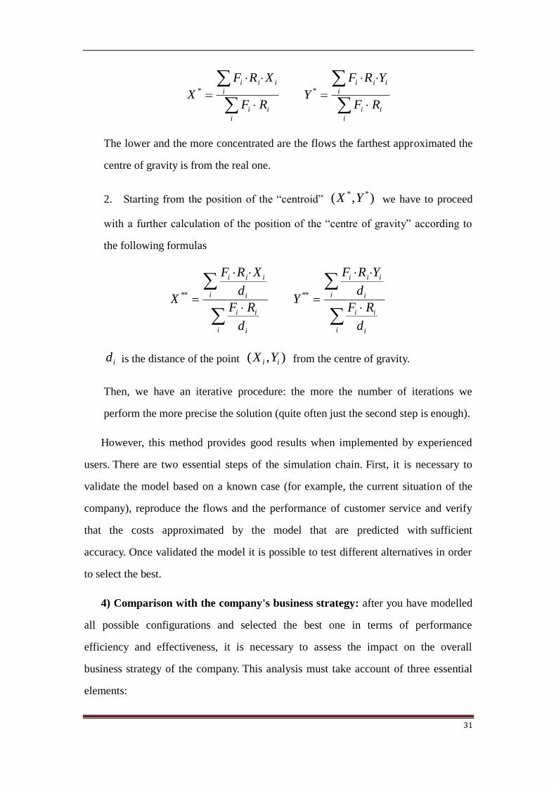
The lower and the more concentrated are the flows the farthest approximated the

centre of gravity is from the real one.

2. Starting from the position of the “centroid” ),( ** YX we have to proceed

with a further calculation of the position of the “centre of gravity” according to

the following formulas

i i

ii

i i

iii

i i

ii

i i

iii

d

RF

d

YRF

Y

d

RF

d

XRF

X ****

id is the distance of the point ),( ii YX from the centre of gravity.

Then, we have an iterative procedure: the more the number of iterations we

perform the more precise the solution (quite often just the second step is enough).

However, this method provides good results when implemented by experienced

users. There are two essential steps of the simulation chain. First, it is necessary to

validate the model based on a known case (for example, the current situation of the

company), reproduce the flows and the performance of customer service and verify

that the costs approximated by the model that are predicted with sufficient

accuracy. Once validated the model it is possible to test different alternatives in order

to select the best.

4) Comparison with the company's business strategy: after you have modelled

all possible configurations and selected the best one in terms of performance

efficiency and effectiveness, it is necessary to assess the impact on the overall

business strategy of the company. This analysis must take account of three essential

elements:

32

Cost of capital: if you expect increases in inventories, new stores, new

equipment, new vehicles the capital becomes necessary, which, in some cases,

may not be available, in some situations, therefore, the financial limits exclude

various strategic alternatives, which might initially seem attractive;

Operating costs: the minimum operating cost is often the main criterion for

choosing between different alternatives. However, in some cases can be accepted

an increase in those costs in exchange for future flexibility;

Customer service: although the different configurations were initially

developed with goals of increasing customer service level, they require careful

consideration in the final phase with respect to performance effectiveness. The

initial balance between efficiency and effectiveness may shift in favour of the first

element in an effort to minimize costs. In such a situation could for example be a

greater demand relocation of inventory close to customers to improve service

reliability.

In our opinion, the limitation of this policy is the lack of a evaluation of strategic

alternatives proposed. Only the final stage, when the configurations selected is

compared with the strategy, emerging issues such as flexibility or customer

service. It‟s clear that in this way it is difficult to assess comprehensive alternative

configurations, in addition, the final evaluation is not to be exhaustive, because they

are not set priorities, and scores of target levels for each element considered important,

but there is merely a rough estimation. It is seems necessary an analysis that takes into

account from the beginning, in a detailed and accurate way with both aspects of an

economic nature, such as costs and the output of the company such as customer

service level, flexibility, labour relations, etc.

1.2.3 Methodology “Integrated Planning Support Framework”

This methodology was developed to overcome the major defects that

characterize most of the systems to support the design of the existing distribution

33

network. The authors start from the observation that in fact all the techniques

proposed in the literature have at least one of the following defects:

Attention is focused on a particular part of supply chain activities;

Focus on the part of the problem of the development of the distribution

network;

Difficult applicability to the real situations, due to the excessive amount of

data required.

The objective of the proposed criterion is therefore to provide comprehensive

support for all the logistics issues involved in developing the distribution network,

bridging the gap between the mathematical abstraction of operations research tools

and the practical problems faced by designers of the network.

The IPSF, which stands for Integrated Planning Support Framework, is based on a

hierarchical approach to design problem in the sub-division, more easily manageable

and highly correlated with each other. For each step there is a specific technique of

analysis and application support.

This system was first developed with attention to the logistics problems to be

solved, and only later, it was thought to the techniques and models to be used to

support each decision. This is because the system must adapt the techniques available.

The proposed methodology is divided into 4 main phases:

Definition of the network structure.

Deployment of the resources across the network.

Specification of the logic of the flow management.

Specification of operations.

1) Definition of network structure: the first step is to design the layout of the

distribution network. We want to determine the number, location, size of facilities

34

and the allocation of customers and suppliers to the different nodes of the system. The

main cost factors that influence the determination of the buoyancy of the network

are fixed costs and transportation costs associated with specific arcs linking the

nodes. The objective is to determine the most efficient location and allocation of

facilities, so that all customers throughout the area covered by the company are

served effectively. The optimization technique proposed in support of this phase is

a linear programming model of mixed location / allocation;

2) Deployment of resources across the network: the goal of this phase is to find

the optimal distribution along the system, inventory, and final assembly activities,

based on the geographical configuration of the network established in the previous

step. Each product is intended for one or more structures, where it is kept in stock and,

where appropriate, assembled. The economies of scale both in transport and in stocks

play an important role at this stage, as well as the coverage of stocks and lead times

required by customers. You must address important strategic issues concerning the

centralization (decentralization) of stocks and the choice between policies “assembly

to order” (ATO) and “assembly to stock” (ATS). These decisions require the solution

of complex trade-off: by centralizing inventory, for example, the increase in transport

costs could exceed the resulting economies of scale, in addition the level of

inventories in a regional warehouse could be lower if it would be supplied by a central

repository rather than from a central transit point only, etc.

Also in support of this phase is a linear programming model proposed;

3) Specification of the logic of the flow management: at this point we want to

determine, for each product, the size of the stocks in each node to ensure the

replenishment lot size and frequency of reorganization. At this stage it is necessary to

ask whether the structure of the network so far designed, is able to guarantee the

service level target within the cost limits set. It is also important to ask whether the

distribution system has sufficient flexibility so it has to be able to cope with

unexpected demands of customers and sudden changes on the market. In support of

35

the decision-making we should consider the various relationships between the existing

logistics system accuracy required by the clients and the level of safety stock, or

between the “economic order quantity” and' “economic transport quantity”. The

designer must consider all of these relationships simultaneously, since they are closely

related. In addition, the basic characteristics of the network, in certain earlier stages,

can now be checked through a sensitivity analysis.

The model in support of this phase has not yet been completed;

4) Specification of operations: with the support of the application developed

specifically for this phase, the designer should be able to tackle questions such as:

choice of procedure by which to ship customers‟ orders;

the way of assembling and sending loads;

rules for programming the final assembly operations;

procedures for stock replenishment;

routing algorithms for vehicles;

policy of selection of the suppliers;

procedures for communicating demand variations to the suppliers;

All the procedures established in this phase should be tested and controlled: in

particular, such policies may be subject to a refinement to minimize costs while

ensuring the fixed level of service. The additional objective of this phase is to

evaluate the specific network configuration in terms of daily activities (operational):

you want to understand the consequences of an operational nature related to the

adoption of a specific spatial distribution, and then evaluate its performance.

Although all the steps are closely related, this does not exclude the possibility to

address them individually. However, in order to avoid suboptimal solutions, you must,

within the limits of time and cost, verify the results obtained with specific

models. The designer should compare the results of each step with different

36

techniques and evaluate if the overall solution is in line with expectations. For

example, the first phase of the methodology uses a simple linear function for the

evaluation of transportation costs: if the configuration of the network resulting in the

next step generates significantly different transport costs, it is necessary to revise the

parameters of the cost function adopted in the model in support of the previous phase.

In order to support the first three phases have been used several types of

optimization models, while the last has been chosen by computer simulation. The

proposed mix ensures the best compromise between the available techniques and is

able to offer strategic insight of the influence of main parameters (marketing, financial,

environmental and government) on the structure of the network. However, the precise

definition of the distribution requires much more information than what optimization

models are able to treat. In other words, to select the best alternative, the designer

should create and evaluate various distribution plans corresponding to different

strategic scenarios. When used in an interactive optimization facilitates the

examination of a wide range of alternatives: different solutions can be examined

under different parameters, such as costs, capacity constraints and customer

demands. It is important to remember that the results of the optimization techniques

should not be interpreted as the best choice of all: in fact, the models are based on a

simplified representation of the real world. This implies that the results, along with

other factors not modelled directly, as the business climate, trade union and political

tensions that characterize the specific country under consideration, be used as

information and support for the designer.

Unlike the policy described in the previous subsection, this methodology is much

more complete and comprehensive as it addresses not only issues of strategic nature,

but also the problems of a more strictly operational. However the policy does not give

a precise indication of the necessary data for the design and even the mode of finding

the same. In addition, there is no comparison of the logistics strategy with corporate

business strategy, which could result in inconsistencies as a result of the

implementation.

37

1.2.4 Ballou’s methodology

Ronald H. Ballou is one of the most famous authors in the field of logistics, he is a

professor of “Logistics Management” in “Weatherhead School of Management, Case

Western Reserve University”, and author of several books including “Business

Logistics Management” and numerous articles for the journals “Journal of Business

Logistics” and “International Journal of Physical Distribution and Logistics

Management”.

According to Baallou distribution network design is a conventional issue in

logistics and has significant impact on the whole supply chain process. In the past two

decades, many contributions involve the topic of distribution network in both

theoretic and practical areas, which mainly focused on the analyses of logistics costs

and case study for specific practitioners respectively (Ballou.1995, Jayaraman, 1998;

Nozick et al., 2001; Payne et al., 2004; Lalwani et al., 2006; Manzini and Gebennini,

2008). Ballou suggested, in support of the distribution network reconfiguration

problem, a methodology divided into several stages, each described below in detail.

38

Figure 2 Flow chart of the Ballou’s methodology

1) Data collection: network planning often requires a considerable amount of

information from different sources. The most important data to be collected include:

a list all company‟s products;

location of customers, stores and factories;

demand divided by product and by geographical area;

freight rates;

Data collecion Analysis of tools to

support the design

Audit the level of

customer service

Organization of the

study

Benchmarking

(validation of the model

used to describe the

case)

Determination of the

network configuration

39

transit time, transmission time and rate of delivery of the order;

storage costs;

costs of production and purchasing (make-or-buy decision);

size of shipment for each product;

level of inventories by geographic location, product and techniques used to

control inventory level;

models of replenishment adopted (frequency, lot size, period of

replenishment);

cost of processing orders;

cost of capital;

customer service;

equipment and facilities available with its capacity limits;

current distribution models.

Many companies do not have logistics information systems capable to generating

the data listed above. It is therefore necessary to find information from all possible

sources, internal and external. The primary source includes all commercial documents

such as sales orders, generally collected on the corporate information system and

document production, purchasing, shipping, storage and handling, constantly checked

and updated by the company. Other important sources of information are represented

by the accounting records, especially with regard to cost, logistics research conducted

internally but also externally, journals, reports of research sponsored by government,

academic journals, judgments and opinions of people who work in the company.

Once you have collected all data deemed necessary, they must be organized, grouped

and aggregated, so as to support the process of network planning. You must decide for

example what is the unit of measurement to be used during the analysis (measures of

weight, volume, currency, etc..) And then to relate all costs to that size, you have to

40

group the products according to the similar characteristics for a more practical

approach to the problem, it is appropriate to establish the profile of orders and

shipments, group customers by geographical area, estimate the costs of internal and

external transport, the costs of structures (fixed costs, storage and handling), the

capacity limits, etc.. It is only then that the details become important information for

the designer.

2) Analysis of tools to support the design: after getting adequate information for

network planning, it is appropriate to analyze the available techniques used to support

different decisions about the design problem. Although many models are developed,

you can classify them into a few categories: techniques based on statistical maps,

spreadsheet, comparison, simulation models, heuristic models, optimization models,

expert systems.

The data collected in the previous step and the tools used to support the different

project phases are combined, with the help of computers, the so-called "Decision

Support System" (DSS). This system provides a valuable aid to decision making,

allowing the user to interact directly with the database, to send data to the models, and

describe the results in the most comfortable and effective. Some DSS provide an

environment in which the designer can interact, allowing complete freedom for the

final choice, in other cases the system may provide the best solution to

implement. The first situation is typical when you have to make more strategic

decisions, while the second characterizes mostly the operational design of the

network;

3) Audit the level of customer service: now starts the planning process itself. A

logical, but often optional, first step in designing the network is to analyze the level of

customer service. This leads to the demand of customers who currently receive

benefits of efficiency and level of service you would like to receive. For this purpose

it is possible to conduct interviews via e-mail or send a questionnaire. The external

audit would be followed by an audit conducted in-house. The objective is to establish

41

the effectiveness of current performance that the company is able to provide and

establish targets for service network design. However the reality is often more

common for the service level goal is set by management or is set equal to the current

one;

4) Organization of the study: the next step typically involves the definition of

the purpose and objectives of the project, the organization of work teams, the

assessment of availability of the required data collection instruments and

procedures. It should be noted that the study team must be formed primarily by people

whose work area may be affected by the results of the project and should also include

all those able to provide valuable insights and opinions. It is particularly useful to

include in the working group responsible for the production and marketing functions.

The tasks in this phase are as follows:

analysis of the present logistics situation in terms of cost, level of service and

logistics, to provide a basis for assessing the potential alternative

configurations. In other words, you must define a reference point for costs and the

level of service, for which the improvements will be evaluated. Furthermore, due

to changed circumstances (freight rates, handling costs and inventory, demand

variations, etc..), this reference point may change over time: it is therefore

necessary to review it periodically;

interview the management and team members to ensure understanding by

everyone of project goals and develop the knowledge necessary to define

alternative logistics systems to be evaluated during the study;

prepare a preliminary list of logistics, marketing policies and guidelines

deemed critical in the evaluation of different alternatives;

specify the criteria for evaluation and study of the output in terms of cost and

service level;

42

select the techniques and instruments deemed suitable for the analysis of

different alternatives, prepare the input data, estimates of costs and time;

to incorporate the specific information requested and provide input to the

procedures;

identify any manual corrections needed to supplement the results of the model,

for a more accurate assessment of the impact of cost and service level;

conduct a group to study the results, conclusions, the criterion for selecting

models, and design the work plan;

estimate the benefits in terms of cost reduction and/or improvement of the

level of service expected from the study;

suggest recommendations for immediate improvements in cost and service;

the method of project management, estimating personnel, computer systems

and other support tools needed for work in progress.

5) Benchmarking: this phase is the validation of the modelling or other analytical

processes adopted during the planning. We want to create a landmark using the

company's current policies and distribution models. The modelling is the most

common approach to the problem of network design and benchmarking plays an

important role in the analytic process. All the study design is to compare the network

in its current configuration with a new and improved structure. Of course

management would reflect that the comparison as much as possible the actual

conditions, but the models are much easier to manipulate than the reality, so the

modelling is adopted in order to make comparisons.

Benchmarking is the process by which it is checked if the modelling process

faithfully reproduces the costs and the level of service corresponding to the current

distribution structure. In this way you are sure that when the model represents a

network configuration not yet experienced in reality, it measures the cost and with

reasonable accuracy the level of service.

43

Benchmarking proceeds as follows: first we establish groupings of representative

products. The optimal number is derived from a compromise between the distinctive

characteristics of products, especially in terms of cost and service, and benefits related

to the reduction of data to be processed, resulting from the aggregation of

products. Then sales are aggregated geographically into a manageable number of

demand centres. We define customer service policies for each group of goods, and

collected data on the most relevant cost categories in the design of the network, such

as transportation, inventory, handling and production/purchase. We define the current

flow of goods and inventory maintenance policies. Finally, we evaluate, from the data

collected, the relationship between costs, demand and service. The information is

organized into categories of cost and service, in order to be compared with the

output. The team analyzes the results to evaluate the correspondence or explain any

deviations. Once the validation process is complete, you can proceed with the

selection of the best configuration distribution;

6) Determination of the network configuration: the modern approach to

planning the configuration of the distribution is to use the computer to manipulate the

huge amount of data involved in the analysis. The models that address the problem of

locating facilities in the network are particularly popular. They are used to answer

questions such as number, size and location of factories and warehouses, to the

allocation of demand nodes; assignment of products to stock in the various

structures. However, there is an integrated model capable of tackling the entire design

problem. It is therefore necessary to break the overall problem in more manageable

parts. In practice, this means determining the location of structures, policies, inventory,

transport planning, etc. separately, but following a recursive approach, so the results

of analysis are used as input to another analysis. The objectives of the reconfiguration

of the network are as follows:

to minimize all relevant logistics costs, while maintaining the service level

objective;

44

to maximize the level of customer service, considering the limitation of fixed

costs;

to maximize profits by maximizing the difference between the revenue from

an increase in the level of service and costs resulting from the performance of

such guarantee of effectiveness.

The third goal is to better grasp the business point of view, however due to the

difficulty connected with the evaluation of the relationship between the increase in the

level of service and increased sales, most of the models are built around the first

objective function.

Often there may be errors in the estimated costs and information as input for

network planning. It is therefore appropriate to conduct a “what-if” analysis, which is

to repeat the analysis to determine the best configuration, using the network scenario

selected and modified cost parameters and capabilities. It‟s a more concrete way to

use the analytic process, which allows a more robust network design and

corresponding to reality. The “what-if” analysis is often considered more valuable

than the models, as it allows the decision-maker to evaluate the optimal solution given

a particular set of data. This is because often there are small differences in cost

between alternative network configurations and because a more robust network design

is often better than the optimal solution from the mathematical point of view.

The proposed methodology is very interesting: they are described in detail and

relevant data for planning, finding sources of data and the means of aggregation, and

tools to support the design of the network, with its advantages and

disadvantages, both the sequential steps to follow when designing. As regards the

latter, the most innovative, first mentioned in the proposed methodology and not

present in the second, is the activity of benchmarking, which reasonably should

precede the application of any analytical tool. Regarding the definition of the

configuration distribution the proposed criterion is rather similar, the global design

problem is divided into several parts, each addressed with the help of simulation

45

models, or heuristic optimization. However, data are not an indication of the

technique to use for each stage, but provides an overview of the tools available,

leaving the designer free to choose.

1.2.5 Distribution network selection matrix

In this research, we focus on the strategic planning of the distribution network

design. The main objective is to optimize the existing distribution network selection

matrix, which aims at finding a rough distribution network structure that fits the

specific distribution problem. The normative distribution network selection matrix is a

tool in order to help the users to make the strategic decision in distribution process.

Hence, making the correct strategic distribution decision depends upon the accuracy

of normative distribution network selection matrix representing the relationship

between distribution problem and distribution solution. The following diagram is the

theoretic construct of existing distribution network selection matrix.

Figure 3 Theoretic model of distribution network selection matrix

Regarding the theory model, the distribution problem can be defined by a range

46

of different drivers. These drivers are classified into four macrodrivers including

product, demand, service and supply characteristics, each macrodriver can describe

one feature of the distribution problem. Furthermore, the four characteristics can be

integrated into two groups based on the different determinants. Hence, the

characteristics of Firm and Market could be use to depict the distribution problem

from macroscopic point of view.

The distribution network solution, or called distribution structure in literature,

involves some issues like number of echelons, number of facilities for each echelon in

the distribution network and type of the facility.

The existing normative distribution network selection matrix was developed by

analyzing the distribution solutions of a number of leading companies, and evaluating

the distribution problems of these companies in a qualitative way, eventually, the

relationship of distribution problem and distribution solution can be represented in a

two-dimension graph. There are two fundamental assumptions in this model. Firstly,

every driver seems to be important to describe the distribution problem. Another

hypothesis is that each driver is perceived has equally weight. In fact, these two

hypotheses may bring the inaccuracy of relationship between distribution problem and

distribution solution. Therefore, this research intends to adopt quantitative approach to

examine and/or improve the accuracy of normative distribution network selection

matrix.

1.3 Mathematical methodologies coupling the selection process

1.3.1 Mathematical methodologies coupling the selection process

To optimize the distribution network selection model, an extensive literature

review on the relevant quantitative approaches was completed. By taking into

consideration the objectives of this research, we need to measure the importance of

the drivers in order to find the more important ones, and obtain a multiple regression

result for these drivers for the sake of making the model to be more accurate.

47

Researchers have developed several methods to measure attribute importance

(Fontenot et al., 2007). Yet, a literature review suggests that logistics researchers have

traditionally used stated importance ratings and statistically inferred importance

analysis.

Logistics researchers usually use stated importance ratings to measure attribute

importance by rating the importance for each attribute from “not important” to

“critically important”, or by using a five-point Scale, where 1 means “no importance”

and 5 means “critical importance”. Many logistics research studies have taken this

approach (Murphy and Poist, 2000; Gibson et al., 2002; Min and Lambert, 2002).

However, although common in practice, this method has major research limitations.

The significant limitation is that stated importance ratings often discriminate poorly

among attributes. Research often finds all attributes to be “critically important”. If all

attributes are found to be “very important”, then the usefulness of research findings is

extremely limited (Garver et al., 2010).

Despite many logistics research studies show little variation in the importance of

attributes when using stated importance, for example, the adoption of a seven-point

scale rating (Crosby and LeMay, 1998), stated importance measures often

discriminate poorly among logistics attributes.

In order to overcome the problem of stated importance ratings, the statistically

inferred importance rating is an effective alternative. In this technique, researchers

correlate or regress attribute performance against a dependent variable, or use factor

analysis or apply an integrated approach to measure the importance of the attributes.

In logistics research, all those methods have been used to infer attribute importance.

For example, Patterson et al. (2003) used structural equation modelling to infer the

importance of key drivers for evaluating the adoption of new technologies on supply

chain management. Zhang et al. (2005) applied structural equation modelling to infer

the importance of attributes on logistics flexibility. Skipper et al. (2009) used

structural equation modelling and regression to examine the importance of risk drivers

48

influencing the supply chain flexibility. Wanke and Zinn (2004) used correlation

analysis and logistic regression analysis to infer the importance of influence on

strategic decision making.

Considering the features of stated importance ratings and statistically inferred

importance ratings, we use an integrated approach consisting of five-point Liker scale,

correlation analysis and factor analysis to carry out the importance measurement of

attributes. To achieve the accuracy of the distribution network selection matrix,

regression modelling can be used in order to figure out the precise value of drivers

after the importance measurement. The literature review suggests that the principal

components regression (PCR) can be better work rather than the least square

regression due to the drivers may highly correlated (Filzmoser, White Paper; Sutter et

al., 1992).

49

Chapter 2. The Selection of Drivers

We found 34 drivers involving four macrodrivers by literature study. In this

section, we will discuss the definition and the measurement method of each driver.

The first part argues the driver‟s implication and the effect on the distribution network.

With regard to the second part, we will demonstrate the measurement method and the

relationship between the driver‟s value and logistics costs.

2.1 Definition of the drivers

Product Characteristics

Variety (number of products)

Variety indicates the amount of different product codes that a company has. It is

measured according to the number of codes commercialized by the company during a

year. The main impact of products variety is related to the number of echelons

decision and the typology of the warehouse (Chopra, 2003). The effect over these two

decisions has to do with the fact that a wide range of products implies a higher level

of stocks and then a higher maintenance cost.

Product Value-Density (PVD)

Product value density is widely recognized as an important factor but has not

received much attention in the academic literature. Value density is highlighted in

particular as a key determinant of the level of centralization, with high value density

products being manufactured at a few large-scale plants. Voordijk (1998) identifies

more centralized inventory holding associated with higher product value densities. As

the value density of a product decreases the percentage of additional distribution costs

increases.

Products that have low value density (coal, iron ore, bauxite, and sand) have low

storage costs but high movement costs as a percentage of their sales price. Inventory

carrying costs are computed as a fraction of the product‟s value. Low product value

50

means low storage cost because inventory carrying cost is the dominant factor in

storage cost. Transport costs, on the other hand, are pegged to weight. When the value

of the product is low, transport costs represent a high proportion of the sales price.

High value density products (electronic equipment, jewelry, and musical

instruments) show the opposite pattern with higher storage and lower transport costs.

This results in a U-shaped total logistics cost curve. Hence, firms dealing with low

value density products frequently try to negotiate more favorable transportation rates.

If the product has a high value density, minimizing the amount of inventory

maintained is a typical reaction.

Physical Density (kg/m3, Weight-Bulk Ratio)

The density of a product is defined as its mass per unit volume. Products of low

physical density offer poor utilization of the storage and transportation system. Such

products include boats, lampshades, and furniture.

The ratio of product weight to bulk is a particularly meaningful measure, as

transportation and storage costs are directly related to them. Products that are dense,

that is, have a high weight-bulk ratio (rolled steel, printed materials, and canned

foods), show good utilization of transportation equipment and storage facilities, with

the costs of both tending to be low. However, for products with low density (inflated

beach balls, boats, potato chips, and lampshades), the bulk capacity of transportation

equipments is fully utilized before the weight-carrying limit is reached. Also, the

handling and space costs, which are weight-based, tend to be high relative to the

product‟s sales prices.

As the product density increases, both storage and transportation costs decline as

a percentage of the sales price. Although price may also be reduced by lower storage

and transportation costs, they are just two cost factor s among many that make up

price. Therefore, total logistics costs can decline faster than price.

51

Risk of Obsolescence (days)

Every product has a specific life cycle, time that can be measured in days, weeks,

months, etc. The risk of obsolescence can be considered either as perishability (time

from the date of production to the date of expiration), for example for fresh goods or

it can be seen as the period of time that a product can be offered to a market which is

determined by changes in the customer‟s needs or due to the launch of a new version

of the product, for example fashion goods and consumer electronics goods.

Contribution Margin

Contribution margin equals price minus variable cost divided by price and is

expressed as a percentage. High profit margin products increase the cost of shortage,

instead low profit margin products force to minimize the physical costs: costs of

production, transportation and inventory storage. These two types of costs determine

the decision about where in the chain to position inventory (Fisher, 1997).

Substitutability

In the case that the product is out of stock, the company could supply another

product to satisfy the same customer need. If the company could not supply another

product in case of out of stock, the customer may immediately go to a competitor to

resource the product (Tim Payne, Melvyn J.Peters, 2004). Substitutability can be

viewed in terms of lost sales to the supplier. Lower substitutability usually means a

greater chance for a customer to select a competing product, thus resulting in a lost

sale for the supplier.

Product Complexity

Level of technology and innovation involved in developing the product, also

includes the level of services involved in supporting the product from production

through distribution and after sales support.

Demand is predictable, the product life cycle long, and the contribution margin

thin for products that are primarily functional. Demand is unpredictable, the product

52

life cycle short, and the contribution margin more generous for products that are

primarily innovative. An innovative product needs a responsive supply chain, a

functional product an efficient one.

Stage of Life Cycle

The concept that products and groups of products advance through a sale cycle of

introduction, rapid growth, maturity, and decline can be useful to strategic logistical

planning. Each stage of the life cycle can mean a different network configuration

would be most economical. Products that are in the introductory stages of the life

cycle may receive limited distribution unless given a promotional push. When

products are in their growth and maturity stages, more extensive distribution in the

form of many stocking points and high stocking levels will likely be the best strategy

when combining revenue and cost considerations. Products in their decline stage,

where sales levels cannot support extensive distribution, are best consolidated into

fewer locations (Ronald H. Ballou, 2007). Christopher and Peck (1999) highlight the

increased importance of a supply chain that delivers reliability where products exhibit

short life cycle.

Handling characteristic

Differences in handling characteristic of products can also impact on distribution

network costs and, therefore the most appropriate distribution network selection. For

example, differences in the level of security or safety requirements of the vehicle can

affect the type of mode or vehicle choice for a product, and can also lead to network

constraints in the type of operation that can be used (Rushton et al.,2000).

Shelf Life (length of shelf life)

Products with a short shelf life would lend themselves to networks that hold low

levels of inventory and utilize faster transport modes (Lovell, Saw, and Stimson,

2005).

53

Value

As supply chain costs are mainly activity driven, and the associated costs are

based on this level of activity, then a higher value orderline (high value product) can

stand a higher amount of activity as it passes along the supply chain, and still produce

a reasonable return (Tim Payne, Melvyn J. Peters, 2004).


Based on the 80-20 concept, the products could be grouped or classified by their

sales activity. The top 20 percent might be called A items, the next 30 percent B items,

and the remainder C items. Each category of items could be distributed differently. A

items might receive wide geographic distribution through many warehouses with high

levels of stock availability, whereas C items might be distributed from a single,

central stocking point with lower total stocking levels than for the A items. B item

would have an intermediate distribution strategy where few regional warehouses are

used.

Competition

The effect of competition in the product line can be an important determinant of

the final placement of warehouses, the stocking levels, and the method of delivery.

Because physical distribution service can have a positive effect on sales, network

configuration is often brought in line with that of competition as a way of avoiding

lost sales. If competition maintains a high service level through close proximity of

warehouses to customers, the network is also likely to conform to that of the

competition (Ronald H. Ballou, 2007).

Production Strategy

The foundation of production strategy is based on identifying four representative

production modes (build-to-stock (BTS), assemble-to-order (ATO), make-to-order

(MTO), and design-to-order (DTO)) that are appropriate for different products

depending on the product‟s characteristics.

54

1) Build-to-stock

BTS is very common because they are appropriate for high volume, low profit

margin, and commodity products. Such products tend to have a relatively stable

demand, which can be forecasted with a low degree of error when accurate

historical demand information is available.

Manufacturers in this production strategy tend to push product into retailers‟

points based on end-product forecasts. The product flow relies heavily on

distribution centers and retailers that deliver products to consumers in the most

cost-efficient manner. If the volume allows it, manufacturers may also make

direct-to-store distribution agreements with large retailers.

This type of production strategy is the most prone to the bullwhip effect and must

relentlessly focus on minimizing costs. For example, warehousing costs are

reduced through the cross-docking concept, while transportation costs are

minimized through the shipment in full truckload, purchasing in large volume can

further increase the efficiency.

2) Assemble-to-order

This kind production strategy provides customers with a limited number of

choices in the configuration of the final product. ATO is typically appropriate for

higher priced consumer goods that are assembled to individual end customer

specifications. These products are also frequently updated with the latest

technologies, increasing their rate of obsolescence, have low profit margins and

tend to operate within very competitive environment.

The ATO logistics process is typically controlled by the firms. These are often

small number of intermediaries in distribution network, with end products either

going to retailers for delivery to the end customer, or directly to the end customer.

The major management issue with the ATO logistics is the need to balance the

pressures of achieving low cost, timely production and delivery while embrace

55

both agile and lean elements in their capabilities.

3) Make-to-order

The MTO production strategy provides consumers with the opportunity to have at

least some part of the product uniquely built to their individual specification.

These products are low volume and high profit margin.

In the logistics process, the smaller number of supply chain intermediaries allows

for a faster response to customer requests, as well as easier sharing of information

among the supply chain partners. To ensure satisfied customers, the logistics

processes of MTO must minimize the delay.

4) Design-to-order

The ability to completely customize a product is the key characteristic of DTO,

resulting in the customer having the greatest amount of input into the finished

product. DTO process allows customers to design the products to meet their

unique individual tastes. Such products are by definition low volume (often one),

with highly variable characteristics, and very high priced. Forecasting is hardly

done at all. There is typically no finished goods inventory in DTO manufacturer

point.

The DTO logistics process is usually controlled by the designer and builder, which

typically deals directly with the end customer, and lead time tends to be long.

DTO logistics must provide its diverse customers with the highest quality of

product and service in a highly uncertain environment.

Service characteristics

Cycle Time

Number of days it takes to deliver an order from the moment it was placed by the

customer till customer receives the goods. The order cycle contains all the

time-related events that make up the total time required for a customer to receive an

56

order. The individual order cycle time elements are order transmittal time,

order-processing time, order assemble time, stock availability, production time, and

delivery time.

The stock availability has a dramatic effect on total order cycle time because it

often forces product and information flows to move out of the established channel. A

normal channel may be to supply customers through a warehouse. When stock is not

available in warehouse inventories, a second, or backup, distribution channel may be

used.

Another primary element in the order cycle over which the logistician has direct

control is the delivery time – the time required to move the order from the stocking

point to the customer location. It may also include the time for loading at the original

point and unloading at the destination point (Chopra, 2003).

Completeness (item fill rate)

It is the probability of having a product in stock when a customer‟s order arrives.

An increase in the required completeness will lead to additional inventory holding at

the decoupling point in the network. This increase in inventories will translate in

additional costs that have to be weighed against the increase in profits. This trade-off

is an important relationship in selecting the most appropriate supply chain for a given

situation. Diversity between products or customer in terms of completeness can,

therefore, influence the most appropriate supply chain selection (Lovell, Saw, and

Stimson, 2005).

Returnability

Returnability represents ease with which a customer can return unsatisfactory

merchandise and the ability of the network to handle such returns.

For some type of products, the possibility to return them become very important,

for example, for electronic goods with parts that has to be disposed through specific

processes or in the case of defective products. By implementing returnability to their

57

products the company becomes responsible of the recollection of all non usable

products and their recycling either to reuse them or to sell as raw material to other

companies.

From a logistics point of view, returnability is the capability of the network to

handle returns depends on the number of levels of the network. In the case of direct

shipment, reverse supply chain will be expensive and difficult to implement (Chopra,

2003).

Accuracy

It represents the capacity of the firm to fulfill orders in the exact way as it was

placed by the customer.

Tracking (order visibility)

It indicates the capacity of the firm to provide relative accurate information about the

state of order in progress, or the ability of the customer to track their order from

placement to delivery (Chopra, 2003).

Customer Experience

Customer experience means ease with which the customer can place and receive

the order (Chopra, 2003).

Punctuality

It measures how accurate the supplier can deliver product to the points of

customers within required cycle time.

Ability to Expedite Orders

Expedited shipments are those that require special delivery in order to reduce the

normal order cycle time. Although expending costs considerably more than standard

delivery, the cost of a lost customer may be even higher (Ronald H. Ballou, 1999).

58

Demand characteristics

Dimension of the Order

The dimension of the order can be classified from the point of view of the

quantity, in different levels: single product, packages, boxes, pallets, truck loads. If

the dimension of the order can saturate the transport unit, the direct delivery from a

central warehouse or factory will be mandatory. The inclusion of intermediate levels

on this case will product an increase of handling and inventory costs without a

reduction in transport costs. With regard to smaller order size, a second echelon will

be required to allow the firm to reach the clients with transport mediums with high

saturation. This way the local delivery costs will be optimized. The most critical

scenario is represented by very small orders with high density of clients. In this case,

a three echelon network must be applied (Archini & Banno, 2003).

Number of Customers

This attribute indicates the total number of customers the company has. The

higher the number of customers, the higher the logistics costs, since it implies a higher

number of deliveries causing an increase in the transportation costs, also in the

handling and order management costs (Archini & Banno, 2003). On the other hand,

this attribute is used to try to assess the risk of obsolescence. If a product has a few

amounts of customers in a year, then it can be described as highly customized.

Frequency of delivery

This driver corresponds to the amount of deliveries for unit of time (day, week,

and month). The frequency of delivery affects the different logistics costs mainly due

to the fact that higher frequencies would imply higher levels of stock causing an

increase in the cost of maintenance. Besides, in order to deliver the products more

frequently to the customer, it is reasonable to think that the product should be closer

to the client, which causes an increase in the stocks. It is important to point out that

usually the volume of the order is lower for high levels of frequency of delivery,

59

impacting in the handling and transportation costs (Archini & Banno, 2003).

Seasonality

Seasonality indicates any predictable change or pattern in a time series that recurs

or repeats over a specific period of time can be said to be seasonal. Seasonality affects

stocking costs by increasing its levels in the seasons it occurs, also increases the

information requirements and the need of flexibility in order to cope with the demand

variations in those periods. If seasonality increases or the product has a high

seasonality there is a tendency of moving towards customers to ensure short delivery

times in periods of maximum requests (Archini & Banno, 2003).


Predictability of demand represents the average margin of error in the demand

forecast at the time production is committed. The effect of demand predictability on

supply chain design is widely discussed in the supply chain literature (Fisher, 1997;

Lovell, Saw, and Stimson, 2005). The predictability of the demand has an impact on

inventory holding policy in relation to the level of inventory centralization within a

supply chain. The higher the level of unpredictability, the more centralized should be

the inventories (Lovell, Saw, and Stimson, 2005).

Spatial Density

The definition of spatial density is that the quantity delivered on each shipment is

directly related with the amount of Point of Sales (or customers) that a company has

by square kilometer.

Demand Volatility

Demand volatility is a measure of overall demand variability. The volatility of a

product is determined by dividing the standard deviation of demand over a 12-month

period with the mean demand. It gives a representation of how variable the demand

pattern is in relation to the average demand. A great volatility shows significant

reductions in service, with associated larger levels of inventory to support that lower

60

service level.

Demand Level

This driver measures the total demand of a product in a specific time period. It

influences factors such as modes of transport and warehouse size and location where

the economies of scale of production or distribution influence supply chain costs.

Supply characteristics

Number of Plants

Number of plants indicates the total number of plants a company has. The

number of plants has an effect over the location of warehouses and the level of

centralization of the warehouses (Lin & Lei, 2009). A large number of plants imply a

larger number of links between the manufacturing point and the warehouses or the

customer in case of direct shipment.


The location of customers and the location of the plants have to be known in

order to calculate the distance. The distance from plant to client affects total logistics

costs since with the increase of distance there is a direct increase of transport cost.

Also the cost of maintenance of inventories varies since with distance increments the

stocks tend to grow due to decentralization.


The definition of level of specialization means the plants produce only one family

of products. As the level of specialization of the plant in a supply chain decrease, the

inventory and resulting inventory cost raise due to decentralization and loss of

economies of scale. On the other hand, if the level of specialization increases, total

transportation cost will also rise by increasing the distance from plant to clients or

warehouses. Facility cost decreases as their number is reduced because consolidation

allows the firm to exploit economies of scale (Chopra, 2003).

61


It is the exclusivity of realization of a product in one plant, or the level of

production concentration in one plant. To some extent, this concept is adverse to level

of specialization.

2.2 Measurement method of the drivers

Product characteristics

Variety (number of products)

The variety of products could be measured directly in number of product codes. It

can be said that with a great variety of products, the criticality of the driver raises and

the distribution network should be centralized in order to avoid duplication and

increase of the level of stock.

Product Value-Density (PVD)

The unit of measurement used for the analysis is Euro/kg, and from the

theoretical explanation above, the products with high value should be considered as

critical for the distribution network design. In this case, a centralized network might

be implemented in order to reduce the level of inventory and its handling cost, but

having the appropriate cycle time to avoid stock out.

Physical Density (kg/m3, Weight-Bulk Ratio)

The density is measured in unit of Kg/ m3. In theory, products having low value

of density should be distributed with a centralized network in order to facilitate

primary transport policy and reduce the amount of space required for inventory.

Risk of Obsolescence (days)

The risk of obsolescence is measured in days. Theoretically, the products with

high risk of obsolescence should be distributed with a centralized network in order to

reduce the cycle time and the level of stock.

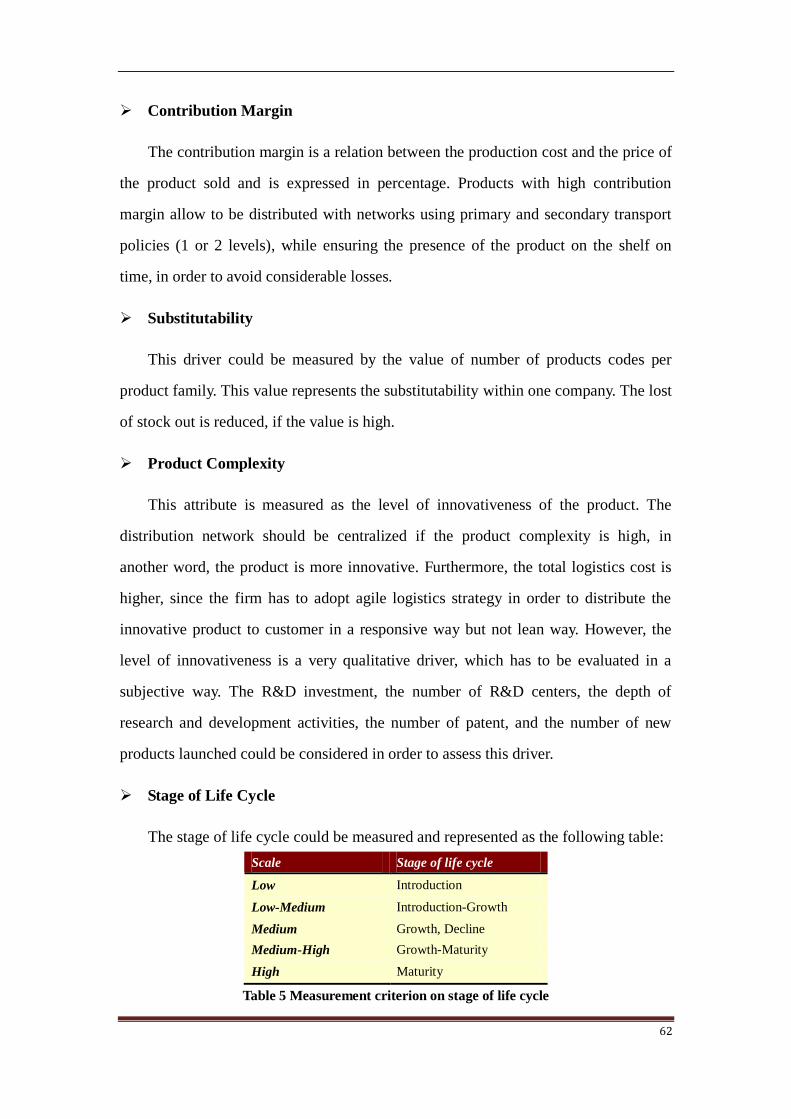
62

Contribution Margin

The contribution margin is a relation between the production cost and the price of

the product sold and is expressed in percentage. Products with high contribution

margin allow to be distributed with networks using primary and secondary transport

policies (1 or 2 levels), while ensuring the presence of the product on the shelf on

time, in order to avoid considerable losses.

Substitutability

This driver could be measured by the value of number of products codes per

product family. This value represents the substitutability within one company. The lost

of stock out is reduced, if the value is high.

Product Complexity

This attribute is measured as the level of innovativeness of the product. The

distribution network should be centralized if the product complexity is high, in

another word, the product is more innovative. Furthermore, the total logistics cost is

higher, since the firm has to adopt agile logistics strategy in order to distribute the

innovative product to customer in a responsive way but not lean way. However, the

level of innovativeness is a very qualitative driver, which has to be evaluated in a

subjective way. The R&D investment, the number of R&D centers, the depth of

research and development activities, the number of patent, and the number of new

products launched could be considered in order to assess this driver.

Stage of Life Cycle

The stage of life cycle could be measured and represented as the following table:

Scale Stage of life cycle

Low Introduction

Low-Medium Introduction-Growth

Medium Growth, Decline

Medium-High Growth-Maturity

High Maturity

Table 5 Measurement criterion on stage of life cycle

63

This driver should be measured in a subjective way. The risk of obsolescence, the

level of innovativeness and the number of new products have deeply impact on this

driver. If the products are highly innovative, which represents the risk of obsolescence

is high, and the company has to launch more new products in order to maintain the

market position only if the research and development ability of the company is high

enough. The result is that many products are on the stage of introduction or decline.


The driver could be measured according to how many handling requirements

must be fulfilled. There are five main handling requirements: Temperature,

shockproof, waterproof, fireproof, specific package (in order to prevent the surface of

product from scratching). The fewer requirements needed by product, the low impact

on the logistics cost.

Scale Handling characteristic

Low 0-1 requirement

Low-Medium 2 requirement

Medium 3 requirement

Medium-High 4 requirement

High 5 requirement

Table 6 Measurement criterion on handling characteristic

Shelf Life (length of shelf life)

This drive is measured in days. The products with short shelf life would bring the

comparative high stock cost and related high handling costs in the logistics process.

Value

The value of a product is measured by price on shelf in unit of Euro.

Theoretically, the total logistics cost is higher if the product with high value.

64


It is hardly to investigate the exactly number of items sold by each business unit

in a company. However, we are able to investigate how many product families

account on top 80 percent sales volume. And then, we figure out the ratio of these

product families to the whole number of product family the company has. The

logistics cost is high if the ABC product characteristic ratio if large.

Competition

The level of competition could be evaluated on the basis of the general

competitiveness on the macro standpoint of industry sector and that of firm‟s point of

view. The level of competition should be high if the competitiveness of industry

sector is aggressive and the company is not at a prior market position. Hence, the

company has to increase the level of inventory and delivery frequency in order to

reduce the probability of stock out and increase the service level.

Production Strategy

The production strategy could be investigated from firm‟s website and/or

interview with production director. In general, the products produced with BTO

strategy has comparative low total logistics costs, while the DTO strategy leads to

comparative high total logistics costs.

Service characteristics

Cycle Time

The cycle time is measured in days. Firms that target customers who can tolerate

a large cycle time require few locations that may be far from the customer and can

focus on increasing the capacity of each location. On the other hand, firms that target

customers that value short cycle time need to locate close to them. These firms must

have many facilities, with each location having a low capacity. Thus, a decrease in

customer‟s desired response time increases the number of facilities required in the

network.

65

Completeness (item fill rate)

This driver is more an internal decision or goal of the firm rather than an effect of

the distribution networks. The total logistics costs may high if the completeness is low,

because this would bring high transportation cost and repeatable distribution

activities.

Returnability

The returnability is measured based on the level of importance of reverse logistics

to the firm. Theoretically, as the percentage of products returned increase, the

criticality of this driver also rise because a more complex network is required.

Accuracy

It can be calculated by dividing the number of correct orders delivered by the

total number of orders placed and expressed in percentage.

Tracking (order visibility)

This driver is measured based on the level of importance of order visibility to the

customer. This attribute has different level of impact on different industries. With

regard to the commodity industry, the order visibility is meaningless, while as to

express industry, this drive is critical to the customer service.

Customer Experience

Customer experience could be measured based on the number of ways through

which the customers can purchase the products. If the company provides more sales

points, the logistics costs should be high due to both high facility cost and

transportation cost, while the customer satisfaction is high.

Punctuality

This driver could be measured based on the percentage of the products could be

delivered to point of customer on time.

66

Ability to Expedite Orders

This driver represents the flexibility of delivery, which indicates if the company

is able to handle the customer‟s urgent and/or unusual delivery requirement. If the

capacity of delivery flexibility is high, the firm could increase the logistics cost while

the cost of lost sales would be decreased and maintain the customer‟s satisfaction. In

fact, the flexibility of delivery is hard to evaluate. We have to measure this driver in a

subjective way by evaluating the ability of company to deal with abnormal delivery

requirement.

Demand characteristics


It is considered the order dimension as a percentage of Full Truck Load. For

example, if the order dimension is only some boxes then it corresponds to 20% of

FTL, if it is pallet then 60% of FTL. The transportation mean could not achieve

saturation when the order dimension is low.

Number of Customers

If the number of customer is high enough, it is considered critical to provide more

facilities in order to reduce the transportation cost.


The frequency of delivery is measured in times per week, for example, if the

delivery is once every two weeks then the frequency is 0.5 times per week. The

logistics costs are high if the frequency of delivery is high. Theoretically, the

distribution network with high frequency of delivery should be decentralized.

Seasonality

The seasonality is measured by the times in a year the sales have a peak and the

length of time, so being:

a) Low: it may be seasonality but it is well known and controlled. For example,

67

a product has a peak in sales from June to August; it only happens one time

in a year and lasts a few months.

b) Low-Medium: seasonality is concentrated in the last third of the year.

c) Medium: peaks in sales occur two times per year.

d) Medium-High: peaks occur two times per year but the duration is longer.

e) High: peaks occur more than two times per year.

The logistics cost is higher, if the seasonality is high. The distribution network should

be centralized in order to cope with the impact.

Predictability of demand (%)

Predictability of demand is measured as percentage of accuracy of the prediction

with the actual demand. If the predictability of demand is low, the total logistics cost

is higher.

Spatial Density

Spatial density is measured based on the number of customers per square

kilometer (#of customer/km2). If the spatial density is low, the local transportation

cost is high compared with high spatial density, because the local delivery cost is

related to the distance from DC to customer area, and the distance between points of

customers. In order to achieve the local transportation economies of scale, the spatial

density should be high since the distance from DC to customer area does not change

whatever the number of customer in a specific area.

Demand Volatility

This driver could be measured like the statement of definition, yet, it is hard to

carry out. Here, we use the change rate of sales to indicate this driver due to the sales

volume reflects the customers‟ demand directly. The average change rate of sales

volume in recent 5 years is the measure of this driver and expressed in percentage.

The demand volatility is high if the change is intensive.

68

Demand Level

We can measure this driver according to the market share of the company in the

specific industry. The larger market share a company has, the higher demand level

would be generated.

Supply characteristics

Number of Plants

The number of plants can be measured directly. When there are many plants, the

total logistics cost increases.


This driver can be measured directly as well. The distance from plant to client is

proportional to the total logistics costs.


If the level of specialization of the plants is high, the logistics cost is higher,

mainly because of the higher distance between plants and clients and also due to the

higher risk of stock out.


This driver could be represented by the ratio of total number of product family to

total number of plants, which represents the number of product family produced in

one plant. The exclusivity is high if the ratio is high.

69

Chapter 3. The Case Studies

We investigated 3 companies involving 16 distribution problems in Consumer

Electronics industry, and 7 companies referring to 16 distribution problems in FMCG

industry. Regarding to every distribution problem, we tried to find out the original

value of each driver we explained in the preceding chapter and convert them into

criticality value based on the related measurement method. The criticality value will

be represented as five-point scale and shown in appendix.

3.1 Data collection of Consumer Electronics Industry

With regard to the Consumer Electronics industry, we investigated HP, Sony and

Samsung by historic data and annual report. Hence, we achieve the original data for

all of the drivers.

3.1.1 Hewlett Packard

HP is a leading global provider of products, technologies, software, solutions and

services to individual consumers, small- and medium-sized businesses (“SMBs”) and

large enterprises, including customers in the government, health and education

sectors.

The operations are organized into seven business segments: Services, Enterprise

Storage and Serves (“ESS”), HP Software, the Personal System Group (“PSG”), the

Imaging and Printing Group (“IPG”), HP Financial Services (“HPFS”), and Corporate

Investment.

MACRODRIVER DRIVER VALUE

PRODUCT

Variety (SKUs) 4000

PVD (euro/kg) 1000

Physical Density (kg/m3) 7.6

Risk of obsolescence (days) 120

Contribution Margin (%) 12

Substitutability (SKUs/family) 118

Product Complexity H

70

Table 7 Original value of drivers in HP

3.1.2 Sony

Sony is a leading manufacturer of audio, video, communications, and information

technology products for the consumers and professional markets. Its motion picture,

television, computer entertainment, music and online business make Sony to be one of

the most comprehensive entertainment and technology companies in the world.

Sony has eight business units, including Consumer Products & Devices,

Networked Products & Services, B2B & Disc Manufacturing, Picture, Music,

Stage of life cycle G&M


(number of handling requirements)

2

Shelf Life (days) 23

Value (euro) 800-1000


(ABC product characteristic ratio, %)

32.4

Competition MH

Production Strategy ATO,MTO

SERVICE

Cycle Time (days) 15

Completeness (IFR) 100

Returnability L

Accuracy (%) 100

Tracking L

Customer Experience MH

Punctuality (%) 100

Ability to Expedite Orders L

DEMAND

Dimension of the order (%FTL) 1

Number of customers 32


(deliveries per week)

5

Seasonality LM

Predictability of demand (%) 95

Spatial Density (#customer/km2) 1.1x10-4

Demand Volatility (%) 14.2

Demand Level (%) >25%

SUPPLY

Number of plants 17

Distance from plant to client 6000

Level of specialization M


(number of product family/plant)

2

71

Financial Service, Corporate, All Other.

Sony has six different distribution problems in Italy, according to the locations of

original points. We would like to name them as SO1, SO2, SO3, SO4, SO5 and SO6.

The first 3 distribution problems are characterized by the same supply and product

drivers, but different demand and service requested by customers; representing 85%

of the total flow of goods. The last 3 distribution problems are characterized also by

same supply and product drivers, which are more sophisticated in technology, and

represent 15% of the total flow.

SO1: provides direct delivery to big customers, which orders are big enough. The

products are TVs, software and CDs produced in Europe plants.

SO2: the same products produced in Europe plants, but the products are

distributed through CW and Transit Points.

SO3: the same products produced in Europe plants and delivered by 2 levels

network like SO2. The difference between this and SO2 is that the deliveries are

done to small clients.

SO4: provides direct delivery from CW to big customers, which orders are big

enough in order to satisfy the saturation of the mean. The products passed

through this channel are supplied by Asia plants. Normally, the value density of

products in this channel is higher than SO1-SO3, and more innovative.

SO5: the same products produced in the Far East plants and delivered by 2 levels

network.

SO6: the same products produced in the Far Ease plants and distributed through

CW for small customers.

72

Table 8 Original value of drivers in Sony


SO1 SO2 SO3 SO4 SO5 SO6

PRODUCT

Variety (SKUs) 400 400 400 800 800 800

PVD (euro/kg) 55 55 55 800 800 800

Physical Density (kg/m3) 160 160 160 643 643 643

Risk of obsolescence (days) 180 180 180 240 240 240

Contribution Margin (%) 10 10 10 14 14 14

Substitutability (SKUs/family) 46 46 46 46 46 46

Product Complexity MH MH MH H H H

Stage of life cycle G&M G&M G&M G&M G&M G&M



2 2 2 2 2 2

Shelf Life (days) 12 12 12 30 30 30

Value (euro) 1000 1000 1000 800 800 800



42.3 42.3 42.3 42.3 42.3 42.3

Competition H H H H H H

Production Strategy MTO MTO MTO MTO MTO MTO

SERVICE

Cycle Time (days) 3 4 2 3 4 2

Completeness (IFR) 100 100 100 100 100 100

Returnability L L L L L L

Accuracy (%) 100 100 100 100 100 100

Tracking L L L L L L

Customer Experience M M M M M M

Punctuality (%) 100 100 100 100 100 100

Ability to Expedite Orders L LM H L LM H

DEMAND

Dimension of the order (%FTL) 1 0.6 0.2 1 0.6 0.2

Number of customers 32 32 2668 32 32 2668



3 2 1 3 2 1

Seasonality M M M LM LM LM

Predictability of demand (%) 90 90 90 90 90 90

Spatial Density (#customer/km2) 1.1x10-4 1.1x10-4 8.9x10-3 1.1x10-4 1.1x10-4 8.9x10-3

Demand Volatility (%) 13.4 13.4 13.4 13.4 13.4 13.4

Demand Level (%) 11.8 11.8 11.8 26 26 26

SUPPLY

Number of plants 5 5 5 7 7 7

Distance from plant to client 1000 1000 1000 9000 9000 9000

Level of specialization H H H M M M

Exclusivity of production in a plant 0.6 0.6 0.6 3.3 3.3 3.3

73

3.1.3 Samsung

Samsung is a digital leader and provides a wide range of home appliance and

digital products. They share a commitment to creating innovative, high quality

products and services that are relied on every day by millions of people and

businesses around the world.

Samsung is comprised of eight independent businesses: Visual Display Business;

IT Solution Business; Digital Appliances Business; Mobile Communication Business;

Telecommunication System Business; Digital Imaging Business; Semiconductor

Business; and LCD Business.

Samsung has 9 different distribution problems in Italy, due to the wide range of

products the company provides. We denominate them SA1-SA9.

SA1: characterized by direct delivery of customized mobile phones and television

decoders from Far East plants to mobile operators or TV providers.

SA2: consist of one level of CW that stores products of the home appliances,

produced in the Far East plants and are forwarded directly to big clients.

SA3: consist of CW that stores home appliances products produced from Far East

plants and 20 transit points that manage this type of products.

SA4: consist of one level of CW that stores audio-video and informatics products

produced in Europe plants and forwarded directly to big clients.

SA5: consist of CW that stores audio-video and informatics products produced in

Europe plants and 20 transit pints that manage these types of products.

SA6: represented by mobile phones those are not delivered directly to mobile

operators, but instead stop at one level of CW and then forwarded directly to big

clients.

SA7: represented by mobile phones, which are not delivered directly to mobile

operators, but instead stop at one level of CW and then at a second level of 150

74

transit points that manage this type of products.

SA8: characterized by air conditioners produced in the Far East plant, stop at one

level of CW and then delivered directly to big clients.

SA9: characterized by air conditioners produced in the Far East plants, stop at

one level of CW and then at a second level of 20 transit points that manage this

type of products and then forwarded to clients.


SA1 SA2 SA3 SA4 SA5

PRODUCT

Variety (SKUs) 50 100 100 700 700

PVD (euro/kg) 1000 13 13 370 370

Physical Density (kg/m3) 1200 110 110 170 170

Risk of obsolescence (days) 90 365 365 180 180

Contribution Margin (%) 30 24 24 14 14

Substitutability (SKUs/family) 16.7 16.7 16.7 41 41

Product Complexity H H H H H

Stage of life cycle G&M Mat. Mat. G&M G&M



2 2 2 2 2

Shelf Life (days) 7 24 24 7 7

Value (euro) 800 455 455 925 925



35.5 35.5 35.5 35.5 35.5

Competition MH MH MH MH MH

Production Strategy MTO MTO MTO MTO MTO

SERVICE

Cycle Time (days) 5 3 5 3 5

Completeness (IFR) 100 95 95 95 95

Returnability L L L L L

Accuracy (%) 95 95 95 95 95

Tracking L L L L L

Customer Experience LM LM LM LM LM

Punctuality (%) 95 95 95 95 95

Ability to Expedite Orders LM LM MH LM MH

DEMAND

Dimension of the order (%FTL) 0.4 0.6 0.4 0.6 0.4

Number of customers 5 35 1160 32 1163



0.25 0.5 1 2 2

Seasonality H L L M M

Predictability of demand (%) 95 95 95 95 95

Spatial Density (#customer/km2) 1.7x10-5 1.2x10-4 3.9x10-3 1.1x10-4 3.9x10-3

75

Demand Volatility (%) 15.9 15.9 15.9 15.9 15.9

Demand Level (%) 24 39.5 39.5 26 26

SUPPLY

Number of plants 7 3 3 7 7

Distance from plant to client 9000 9000 9000 1000 1000

Level of specialization H H H H H

Exclusivity of production in a plant 1.4 0.7 0.7 3.3 3.3


SA6 SA7 SA8 SA9

PRODUCT

Variety (SKUs) 50 50 150 150

PVD (euro/kg) 1000 1000 90 90

Physical Density (kg/m3) 1200 1200 170 170

Risk of obsolescence (days) 90 90 365 365

Contribution Margin (%) 30 30 14 14

Substitutability (SKUs/family) 16.7 16.7 30 30

Product Complexity H H H H

Stage of life cycle G&M G&M Mat. Mat.



2 2 2 2

Shelf Life (days) 7 7 24 24

Value (euro) 200 200 1530 1530



35.5 35.5 35.5 35.5

Competition MH MH MH MH

Production Strategy MTO MTO MTO MTO

SERVICE

Cycle Time (days) 3 5 3 5

Completeness (IFR) 95 95 95 95

Returnability (%) L L L L

Accuracy (%) 95 95 95 95

Tracking L L L L

Customer Experience LM LM LM LM

Punctuality (%) 95 95 95 95

Ability to Expedite Orders M H LM MH

DEMAND

Dimension of the order (%FTL) 0.4 0.2 0.6 0.4

Number of customers 32 1163 35 1160



1 1 0.5 1

Seasonality H H L L

Predictability of demand (%) 95 95 95 95

Spatial Density (#customer/km2) 1.1x10-4 3.9x10-3 1.2x10-4 3.9x10-3

Demand Volatility (%) 15.9 15.9 15.9 15.9%

Demand Level (%) 20.6 20.6 39.5 39.5%

76

Table 9 Original value of drivers in Samsung

3.2 Data collection of FMCG Industry

As for the FMCG industry, 7 companies are investigated. We are not able to find

the original data of every driver for all of the distribution problems since some data

are hardly to evaluate or there is few relative information on the annual report and

official website.

3.2.1 Nestle Italia

Nestle is the largest food and nutrition company in the world food and nutrition

company in the world. Founded in1886 by Henri Nestle in Vevey, Switzerland. The

company significantly during the First World War and again following the Second

World War, eventually expanding its offerings beyond its early condensed milk and

infant formula products. Today, the company operates in 86 countries around the

world, and employs over 280000 people.

Nestle Italia is a company‟s branch in Italy established in December 2002. All the

data regarding the company is provided in the table given below. Nestle Italia has 5

Business Units. Each of the units represents its own distribution problem. These

Business Units are:

Nestle1: Food & Nutrition Business Unit. The distribution network is

presented by 2 echelons. In the first echelon there are 2 warehouses that

distribute the goods among 26 warehouses/transit points that create the second

echelon of the network.

Nestle 2: Pasta & Slices Business Unit. The 2 level distribution network is

presented by 3 warehouses in the first echelon and 24 warehouses/transit

points in the second one.

SUPPLY

Number of plants 7 7 7 7

Distance from plant to client 9000 9000 9000 9000

Level of specialization H H H H

Exclusivity of production in a plant 0.4 0.4 0.7 0.7

77

Nestle 3: Confectionery Business Unit. The distribution network in this case is

also presented by 2 levels. 2 warehouses in the firsts level and 34

warehouses/transit points in the second one;

Nestle 4: Bakery Business Unit. 2 levels network with 2 and 28

warehouses/transit points in the first and second levels respectively.

Nestle 5: Foodservices Business Unit. The distribution network composed by

2 warehouses in the first level and 24 warehouses/transit points in the second

one.


Nestle1 Nestle2 Nestle3 Nestle4 Nestle5

PRODUCT

Variety (# of products) 620 357 944 374 830

PVD (euro/kg) 5.6 -

32.10

1.15 -

2.53

8.44 -

14.72 4.9 5.4

Physical Density (kg/m3) 323 253 212 178 196

Risk of Obsolescence (days) 690 365 -1200 190 - 630 150 300

Contribution Margin (%) 18.1 12.3 13.8 12.3 14

Subsitutability (SKUs/product family) >620 >357 >944 >374 >830

Product Complexity (func vs innov) L L L L L

Stage of Life Cycle Mat Mat Mat Mat Mat

Handling characteristic L L H H L

Shelf Life (days) 210 180 150 30 200

Level of Competition (qual) H H H H H

Production Strategy BTS BTS BTS BTS BTS

SERVICE

Cycle Time (days) 6 5.9 5.5 1.5 4

Completeness (Item fill rate, %) 98 98 98 98 98

Accuracy (%) 97 97 97 97 97

Tracking (qual) H H H H H

Customer Experience (qual) H H H H H

Punctuality (%) 90 90 90 90 90

DEMAND

Dimesion of the order 2.4 UL 15 UL 0.5 UL 1.5 UL 1 UL

Number of Customer 11424 11424 26000 5700 22660

Delivery Frequency

(#of delivery/week) 0.23 0.07 0.25 0.28 0.16

Seasonality (qual) L L H H L

Predictability of Demand (%) H H H H H

Spatial Density (#of customer/km2) 379x10-4 379x10-4 863x10-4 189x10-4 752x10-4

SUPPLY

Number of Plants 1 2 1 2 1

Distance from plant to client(km) 600 600 600 600 600

78

Table 10 Original value of drivers in Nestle

3.2.2 Calzedonia

Calzedonia is a relatively young Italian company that was established in 1987

close to Verona. The company produces and sells underwear (brand intimissimi) and

clothes (brand calzedonia). The detailed information about the company is given in

the table below. Considering the fact that the company operates in a fashion, highly

seasonal and hard predictable market and has 2 lines of brands we can distinguish two

distribution problems the company has:

Calz1: Brand line Calzedonia. The distribution network consists of 1 Central

Warehouse.

Calz2: Brand line Intimissimi. The network is composed by 1 level with 1

Central Warehouse.

Level of Specialization Depends on the country/region, but tending to become MH

Exclusivity of production in a plant MH MH MH MH MH


Calz1 Calz2

PRODUCT

Variety (# of products) 3500 3500

PVD (euro/kg) 50 50

Physical Density (kg/m3) 160 160

Risk of Obsolescence (days) 180-sever

al years 180-360

Contribution Margin (%) 38.4 46.2

Subsitutability (SKUs/product family) >3500 >3500

Product Complexity (func vs innov) L ML

Stage of Life Cycle Mat Mat

Handling characteristic L L

Shelf Life (days) 90 - 360 30 - 180

Level of Competition (qual) H MH

Production Strategy BTS BTS

SERVICE

Cycle Time (days) 3 3

Completeness (Item fill rate, %) 99.9 99.9

Accuracy (%) 99.9 99.9

Tracking (qual) Not

available

Not

available

79

Table 11 Original value of drivers in Calzedonia

3.2.3 Reckitt Benckiser

Reckitt Benckiser is a global consumer goods company located in Slough, UK. It

is the world largest produser of the household products and the major producer of

consumer healthcare and personal products. Its brands include Dettol (the world‟s

largest-selling antiseptic), Strepsils (the world‟s largest selling sore throat medicine),

Veet (the world‟s larges selling depilatory brand), Air Wick (the world‟s second

largest-selling air freshener), Calgon, Cilit, Bang, Durex and Vanish. It has operations

in over 60 countries and its products are sold in over 180 countries around the globe.

More detailed information about the company is provided in the table below.

The distribution network of the company composed by 2 levels with more than

20 warehouses in the firsts echelon and more than 130 warehouses/transit points in

the second one.

Customer Experience (qual) MH MH

Punctuality (%) 99.9 99.9

Ability to Expedite Orders No No

DEMAND

Dimesion of the order 0.27m3 0.27m3

Number of Customer 1400 1400

Delivery Frequency (#of delivery/week) 3 3

Seasonality (qual) MH H

Predictability of Demand (%) MH MH

Spatial Density (#of customer/km2) 6.3x10-4 6.3x10-4

SUPPLY

Number of Plants 6 2

Distance from plant to client(km) >1000 >1000

Level of Specialization H H

Exclusivity of production in a plant 1 MH


PRODUCT

Variety (# of products) 800

PVD (euro/kg) 28.05

Physical Density (kg/m3) 375

Risk of Obsolescence (days) 800

Contribution Margin (%) 26.4

Subsitutability (SKUs/product family) >800

80

Table 12 Original value of drivers in Reckitt Benckiser

3.2.4 Coca-Cola Italia

The Coca-Cola Company is an American multinational beverage corporation and

manufacturer, retailer and marketer of non-alcoholic beverage concentrates and

syrups. The company is best known for its flagship product Coca-Cola, invented in

1886 by pharmacist John Stith Pemberton in Columbus, Georgia.[3] The Coca-Cola

formula and brand was bought in 1889 by Asa Candler who incorporated The

Coca-Cola Company in 1892. Besides its namesake Coca-Cola beverage, Coca-Cola

currently offers more than 500 brands in over 200 countries or territories and serves

over 1.7 billion servings each day. Detailed information related to the Italian branch is

given below.

The distribution network of Coca-Cola Italia is presented by 10 warehouses in the

1st echelon and more than 100 transit points in the 2

nd one.

Product Complexity (func vs innov) L

Stage of Life Cycle Mat

Handling characteristic L

Shelf Life (days) 360

Level of Competition (qual) MH

Production Strategy BTS

SERVICE

Cycle Time (days) 3

Completeness (Item fill rate, %) 100

Accuracy (%) 99

Tracking (qual) H

Customer Experience (qual) H

Punctuality (%) 95

DEMAND

Dimesion of the order 0.5 Unit Load

Number of Customer 1600

Delivery Frequency (#of delivery/week) 2

Seasonality (qual) L

Predictability of Demand (%) H

Spatial Density (#of customer/km2) 53x10-4

Demand Variability (%) 21

SUPPLY

Number of Plants 6

Distance from plant to client(km) 1000 - 1200

Level of Specialization ML

Exclusivity of production in a plant 0.5

http://en.wikipedia.org/wiki/The_Coca-Cola_Company#cite_note-2

81

Table 13 Original value of drivers in Coca-Cola

3.2.5 3M

3M formerly known as the Minnesota Mining and Manufacturing Company.

It is an American multinational conglomerate corporation based in Maplewood,

Minnesota, United States.

With over 80,000 employees, they produce a wide range of products (more than

55,000 products), including: adhesives, abrasives, laminates, passive fire protection,

dental products, electronic materials, medical products, car care products (such as sun

films, polish, wax, car shampoo, treatment for the exterior, interior and the under


PRODUCT


PVD (euro/kg) 0.8 - 2


Risk of Obsolescence (days) 365


Subsitutability (SKUs/product family) 130

Product Complexity (func vs innov) L


Handling Characteristics L

Shelf Life (days) 180 - 270

Level of Competition (qual) H


SERVICE

Cycle Time (days) Not available

Completeness (Item fill rate, %) 2.4 weeks of Stock Out

Tracking (qual) H

Customer Experience (qual) H

DEMAND

Dimesion of the order 15 UL


Delivery Frequency (#of delivery/week) 0.3

Seasonality (qual) H


Spatial Density (#of customer/km2) 0.0995x10-4

SUPPLY

Number of Plants 6

Distance from plant to client(km) 500

Level of Specialization L

Exclusivity of production in a plant L

http://en.wikipedia.org/wiki/Multinational_corporation

http://en.wikipedia.org/wiki/United_States

82

chassis rust protection), electronic circuits and optical films. 3M has operations in

more than 60 countries – 29 international companies with manufacturing operations,

and 35 with laboratories. 3M products are available for purchase through distributors

and retailers in more than 200 countries, and many 3M products are available online

directly from the company. Detailed information about the company is given in the

table below.

In 3M we can distinguish 4 distribution problems (one problem for one Business

Unit):

3M1: Health & Care. The distribution network consists of 1 echelon with 5

warehouses in it.

3M2: Consumer & Office. The network is presented by 2 echelons with 5

warehouses in the 1st and 10-15 warehouses/transit points in the 2

nd one.

3M3: Industrial Market. The network is composed by 1 echelon with 5

warehouses in it.

3M4: TGS. This Business Unit is engaged in producing metal signs. The

distribution network is presented by 1 echelon with 5 warehouses in it.


3M1 3M2 3M3 3M4

PRODUCT


PVD (euro/kg) MH L M ML

Physical Density (kg/m3) M ML MH M

Risk of Obsolescence (days) L L L L

Contribution Margin (%) 31.44 21.55 17.41 23.63

Subsitutability (SKUs/product family) >MH >L >M >ML

Product Complexity (func vs innov) H L MH L

Stage of Life Cycle Mat Mat Mat Mat

Handling characteristic M L L L

Shelf Life (days)

Level of Competition (qual) MH H H H

Production Strategy ATO/MTO BTS ATO BTS

SERVICE Cycle Time (days) 3 3 3 3

Accuracy (%) 70 70 70 70

83

Table 14 Original value of drivers in 3M

3.2.6 Unilever Bestfoods

Unilever Bestfoods is a part of Unilever Company that is focused on mayonnaise

and other food products. The company has 2 main Business Units targeted on

HORECA (Hotels, Restaurants and Cafes) and Retail chains respectively. Distribution

network for HORECA Business Unit is presented by 2 echelons with 20 warehouses

in the first echelon and 10 transit points in the second one. Retail Business Unit‟s

network composed just 1 echelon with 20 warehouses in it. Detailed information

about the company is provided in the table below.

Customer Experience (qual)

Punctuality (%) 90 90 90 90

DEMAND

Dimesion of the order

some

packages -

UL

some

packages

some

packages

some

packages

Number of Customer 2000 6500 6000 2500

Delivery Frequency

(#of delivery/week) 0.37 0.37 0.37 0.37

Seasonality (qual) H H H H

Spatial Density (#of customer/km2) 800x10-4

SUPPLY

Number of Plants 50

Distance from plant to client(km) 1100 1100 1100 1100

Exclusivity of production in a plant H H H H


Unil1 Unil2

PRODUCT

Variety (# of products) 200 300

PVD (euro/kg) 7 7.5

Physical Density (kg/m3) MH MH

Risk of Obsolescence (days) 365 -

1500 365 - 750

Contribution Margin (%) 15 14.4

Subsitutability (SKUs/product family) >200 >300

Product Complexity (func vs innov) L L

Stage of Life Cycle Mat Mat

Handling characteristic H H

Shelf Life (days) 450 400

Level of Competition (qual) H H

Production Strategy BTS BTS

84

Table 15 Original value of drivers in Unilever Bestfoods

3.2.7 Hackman

Hackman is a cutlery and cookware company founded in Finland in

1790. Nowadays the Hackman brand is owned by Iittala Group, which was acquired

by Fiskars Corporation in 2007. Hackman is a prestigious brand name in Finland;

according to a 2008 survey which included both Finnish and international brands, it

was the fifth most respected brand among consumers. The distribution network is

very different from the traditional one and composed by 2 echelons with 3

warehouses in the first echelon (central warehouses in Finland, Sweden and Norway)

and just 1 transit point in the second echelon in Norway. The detailed information

about the company is given in the table provided below.

SERVICE

Cycle Time (days) 7.5 5

Completeness (Item fill rate, %) 98 95

Accuracy (%) 90 90

Tracking (qual) H H

Customer Experience (qual) H H

Punctuality (%) 90 90

Ability to Expedite Orders Yes No

DEMAND

Dimesion of the order 1 UL 1Transport Unit

Number of Customer 7000 1000

Delivery Frequency (#of delivery/week) 0.25 0.25

Spatial Density (#of customer/km2) 230x10-4 33x10-4

SUPPLY

Number of Plants 3 2

Distance from plant to client(km) 1200 1200

Level of Specialization H H

Exclusivity of production in a plant MH H


PRODUCT

Variety (# of products) Wide

PVD (euro/kg) 39


Risk of Obsolescence (days) L


Subsitutability (SKUs/product family) Wide

Product Complexity (func vs innov) M

85

Table 16 Original value of drivers in Hackman


Handling characteristic ML

Shelf Life (days) L

Level of Competition (qual) MH


SERVICE

Cycle Time (days) Not available

Completeness (Item fill rate, %) 98

Accuracy (%) 95

Tracking (qual) MH

Customer Experience (qual) M

DEMAND

Dimesion of the order 1 UL up to Transport Unit


Seasonality (qual) H


Spatial Density (#of customer/km2) Not very high

Demand Variability (%) ML

SUPPLY

Number of Plants 5

Distance from plant to client(km) 820 - 1500

Level of Specialization H

Exclusivity of production in a plant H

86

Chapter 4. The Description of Mathematical Methodology

We have presented the whole methodology in the executive summary. Driver list

updating and data collection have been demonstrated in the above chapters. Hence,

the accent of this chapter is on the description of the mathematical methodology.

We will describe the quantitative research procedure on the first part of this

section and introduce the features of each main mathematical approach used in this

study on the second part. The mathematical analysis is the prominent emphasis

distinguishing from the previous relative research. Hence, the correctness of the

mathematical methodology is crucial to the research as a whole.

4.1 The main procedure of mathematical analysis

With regard to the quantitative analysis, the objective is to make the relationship

between distribution problem and distribution solution to be more accurate. Therefore,

we have to adopt some mathematical tools. Through the literature study, we can found

that some inferred statistics models can realize this purpose. The following diagram is

the procedure of mathematical analysis in which three main processes include

reducing the number of drivers, generating the regression function and obtaining the

accurate relationship between distribution problem and distribution solution. The

detailed application of this procedure will be shown in the next chapter.

Figure 4 The procedure of mathematical analysis

87

According to the previous chapters, there are 34 drivers associated to the product,

service, demand and supply characteristics have been found. By taking into consider

the natures of Consumer Electronics industry and FMCG industry, we should find the

drivers that are more able to describe those characteristics for two industries

respectively. Hereby, we need to remove some drivers that are not significant to the

Consumer Electronics industry and FMCG industry.

Firstly, we use descriptive statistics analysis and correlation analysis to see which

drivers can be deleted and/or combined based on their standard deviation and

correlation factor. The drivers have to be cut off in case the value of standard

deviation is zero, since the value is meaningless to the inferred statistics model. The

correlation factor can depict the relation between two variables. The driver can be

neglected if it is highly related to another one whose concept is wilder.

The following step is to use the inferred statistics model to carry out the further

statistical analysis. The confirmatory factor analysis (CFA) can reduce the number of

drivers based on the group of drivers rather than the pair of drivers. Consequently, we

can remove more drivers on this step.

Thanks to the preceding process, we can obtain some more important drivers for

different industries. The second process is to figure out the regression function for

those drivers and obtain their regression coefficients. By taking into consideration the

multicollinearity may exist among the drivers, we have to use principal component

regression (PCR) model to solve this problem.

Finally, the relationship between distribution problem and distribution solution

can be achieved if we put the original critical value of the necessary drivers into the

regression function to figure out the value of Market and Firm characteristics for each

distribution problem, and represent their value on the two-dimension diagram.

88

4.2 The description of mathematical tools

4.2.1 Descriptive statistics

Descriptive statistics quantitatively describes the main features of a collection of

data (Introductory Statistics, 1995). In a research study we may have lots of measures.

Or we may measure a large number of people on any measure. Descriptive statistics

help us to simply large amounts of data in a sensible way. Each descriptive statistic

reduces lots of data into a simpler summary.

Descriptive statistics are distinguished from inferential statistics (or inductive

statistics), in that descriptive statistics provide simple summaries about the sample

and the measures, rather than use the data to learn about the population that the data

are thought to represent. With descriptive statistics we are simply describing what is

or what the data shows. With inferential statistics, we are trying to reach conclusions

that extend beyond the immediate data alone. Thus, we use inferential statistics to

make inferences from our data to more general conditions; we use descriptive

statistics simply to describe what's going on in our data. This generally means that

descriptive statistics, unlike inferential statistics, are not developed on the basis of

probability theory.

Descriptive statistics include the numbers, tables, charts, and graphs used to

describe, organize, summarize, and present raw data. Descriptive statistics are more

often used to examine:

Central tendency - location of data, i.e. where data tend to fall, as measured by

mean, median, and mode.

Dispersion – variability of data, i.e. how spread out data are, as measured by the

variance and its square root, the standard deviation.

Skew – symmetry of data, i.e. how concentrated data are at the low or high end of

the scale, as measured by the skew index.

http://en.wikipedia.org/wiki/Data

http://en.wikipedia.org/wiki/Statistical_inference

http://en.wikipedia.org/wiki/Inductive_statistics

http://en.wikipedia.org/wiki/Inductive_statistics

http://en.wikipedia.org/wiki/Statistical_population

http://en.wikipedia.org/wiki/Probability

89

Kurtosis – peak of data, i.e. how concentrated data are around a single value, as

measured by the kurtosis index.

Descriptive statistics are recommended when the objective is to describe and

discuss a data set more generally and conveniently than would be possible using raw

data along. They are routinely used in reports which contain a significant amount of

qualitative or quantitative data. Descriptive statistics help summarize and support

assertions of fact (Data Analysis, 1995).

A thorough understanding of descriptive statistics is essential for the appropriate

and effective use of all normative and cause-and-effect statistical techniques,

including hypothesis testing, correlation, and regression analysis. Unless descriptive

statistics are fully grasped, data can be easily misunderstood and, thereby,

misrepresented.

In this study, the primary purpose of the application of descriptive statistics is to

summarize the drivers in order to reduce the number of them. Hence, we examine the

central tendency and disperse of the data. Even if the four descriptions of data set

mentioned above are suggested to be examined in literature, the characteristics of

skew and kurtosis do not make any sense in our research. Since statistical analysis

software and most spreadsheets generate all required descriptive statistics, computer

applications offer the best means of preparing such information. We use Excel

application of Microsoft Office, to implement the descriptive statistics.

4.2.2 Correlation analysis

Correlation is a statistical technique that can show whether and how strongly

pairs of variables are related. Like all statistical techniques, correlation is only

appropriate for certain kinds of data. Correlation works for quantifiable data in which

numbers are meaningful, usually quantities of some sort. It cannot be used for purely

categorical data, such as gender, brands purchased, or favorite color.

A correlation coefficient (r) is a statistic used for measuring the strength of a

90

supposed linear association between two variables; that is, how well changes in one

variable can be predicted by changes in another variable. It ranges from -1.0 to +1.0.

The closer r is to +1 or -1, the more closely the two variables are related:

+1 representing absolute positive linear relationship (X increases, Y increases).

-1 representing absolute inverse relationship (X increases, Y decreases).

0 representing no linear relationship (X and Y have no pattern).

Before making any decisions based upon correlation analysis, one must

recognize that correlation does not imply one variable is responsible for the

movement of another. Correlation simply measures the relationship of movement

between two variables (Correlation Analysis, 2007).

In this thesis, one driver can be removed if the correlation coefficient is high

enough, or two drivers are combined into one new attribute. Microsoft's Excel

spreadsheet program can analyze the level of correlation between two variables

through its data analysis function.

4.2.3 Confirmatory factor analysis

Factor analysis is a collection of methods used to examine how underlying

constructs influence the responses on a number of measured variables. The main

applications of factor analytic techniques are: (1) to reduce the number of variables

and (2) to detect structure in the relationships between variables. Therefore, factor

analysis is applied as a data reduction or structure detection method

There are basically two types of factor analysis: exploratory and confirmatory.

Exploratory factor analysis (EFA) attempts to discover the nature of the contracts

influencing a set of responses.

Confirmatory factor analysis (CFA) tests whether a specified set of constructs is

influencing response in a predicted way.

91

The primary objectives of an EFA are to determine (1) the number of common

factors influencing a set of measures in order to identify the nature of the constructs

underlying responses in a specific content area and (2) the strength of the relationship

between each factor and each observed measure.

However, confirmatory factor analysis (CFA) is able to determine if the number

of factors and the loading of measured (indicator) variables on them conform to what

is expected on the basis of pre-established theory. Measured variables are selected on

the basis of prior theory and factor analysis is used to see if they load as predicted on

the expected number of factors. The research‟s priori assumption is that each factor is

associated with a specific subset of measured variables. A minimum requirement of

confirmatory factor analysis is that one hypothesis beforehand the number of factors

in the model, but usually also the research will posit expectations about which

variables will load on which factors.

As for our study, the predefined factor model in which there are four factors is

shown in chapter 1. Our purpose is to examine the strength between the variables and

related factor in order to delete those variables which are less significant to the

factors.

There are two approaches for confirmatory factor analysis:

a) The traditional method. Confirmatory factor analysis can be accomplished through

any general-purpose statistical package which supports factor analysis. Note that

for SEM CFA one uses principle axis factoring (PAF) rather than principle

component analysis (PCA) as the type of factoring. This method allows the

researcher to examine factor loadings of measured variables to determine if they

load on latent variables as predicted by the researcher‟s model.

b) The SEM approach. Confirmatory factor analysis can mean the analysis of

alternative measurement models using a structural equation modeling package

such as AMOS or LISREL. While SEM is typically used to model causal

relationship among latent variables, it is equally possible to use SEM to explore

92

CFA measurement models. This is done by removing from the model all straight

arrows connecting latent variables, adding curved arrows representing covariance

between every pair of latent variables, and leaving in the straight arrows from

each latent variable to its measured variables as well as leaving in the straight

arrows from error and disturbance terms to their respective variables. Such a

measurement model is run like any other model and is evaluated like other models,

using goodness-of-fit measures generated by SEM package.

For data analysis in this research, LISREL was used to perform confirmatory

factor analysis. Using LISREL for confirmatory factor analysis provides a more

rigorous assessment of the fit between the collected data and the theoretical factor

structure.

4.2.4 Principal component regression

Regression analysis includes any techniques for modeling and analyzing several

variables, when the focus is on the relationship between a dependent variable and one

or more independent variables. Regression analysis helps one understand how the

typical value of the dependent variable changes when any one of the independent

variables is varied, while the other independent variables are fixed.

In statistics, principal component regression (PCR) is a regression analysis that

combines principal component analysis (PCA) and linear regression when estimating

regression coefficients. Linear regression is a type of regression analysis to be studied

rigorously, and to be used extensively in practical applications. This is because

models which depend linearly on their unknown parameters are easier to fit than

models which are non-linearly related to their parameters and because the statistical

properties of the resulting estimators are easier to determine. Principal component

analysis is a mathematical procedure that uses an orthogonal transformation to

convert a set of observations of possibly correlated variables into a set of values of

uncorrelated to make a kind of regularized estimation. Therefore, PCR is a procedure

used to overcome problems which arise when the variables are close to being colinear.

http://en.wikipedia.org/wiki/Dependent_variable

http://en.wikipedia.org/wiki/Independent_variable

http://en.wikipedia.org/wiki/Statistics

http://en.wikipedia.org/wiki/Regression_analysis

http://en.wikipedia.org/wiki/Regression_analysis

http://en.wikipedia.org/wiki/Regularization_%28mathematics%29

http://en.wikipedia.org/wiki/Colinear

93

PCR (principal components regression) is a regression method that can be divided

into three steps:

1. The first step is to run a principal components analysis on the table of the

explanatory variables,

2. The second step is to run an ordinary least squares regression (linear

regression) on the selected components: the factors that are most correlated

with the dependent variable will be selected

3. Finally the parameters of the model are computed for the selected explanatory

variables.

We can achieve the drivers‟ regression function and regression coefficients by

using PCR model in order to get rid of the problem of multicollinearity. Regarding the

application of this model, the most of statistics software can support the

implementation of PCR. We use SPSS to carry out the PCR analysis due to the

simplicity on usage.

http://en.wikipedia.org/wiki/Principal_components_analysis

http://en.wikipedia.org/wiki/Ordinary_least_squares

http://en.wikipedia.org/wiki/Linear_regression

http://en.wikipedia.org/wiki/Linear_regression

94

Chapter 5. Application of the Mathematical Models

In this chapter, we present the application of the mathematical models based on

the procedure we showed in the previous section. At the end of this chapter, we will

obtain a series of the drivers that are more important and carry out the further analysis

in order to get the relationship between distribution problem and distribution solution.

5.1 Application in Consumer Electronics Industry

5.1.1 Descriptive statistics analysis

Description of drivers associated product macrodriver

As for the electronic industry, the products are comparative highly innovative and

the level of competition is high as well. On the other hand, the most of products we

investigated are on the growth and mature stage of the whole life cycle. Therefore,

these three related drivers‟ mean value is higher than 4, which is the highest in

product marcodriver group.

With regard to the standard deviation, we can see the value of handling

characteristic is zero, indicating the criticality value of the every sample is totally

same. We have to remove this attribute from the driver list, because correlation

analysis does not work on this driver if the standard deviation is zero.

Driver Mean Std.Dev

Variety 2.25 1.39

Physical Value Density 2.94 1.65

Physical Density 2.69 1.14

Risk of Obsolescence 2.75 1.44

Contribution Margin 2.31 1.01

Substitutability 3.25 1.44

Product Complexity 4.81 0.40

Stage of Life Cycle 4.25 0.45

95

Handling characteristic 2.00 0.00

Shelf Life 3.13 1.63

Value 3.19 1.22

ABC product characteristic 3.38 0.50

Level of Competition 4.38 0.50

Production Strategy 3.94 0.25

Table 17 Descriptive statistics result 1 in Consumer Electronics industry

Description of drivers associated service macrodriver

As the following table shows, the mean value and standard deviation of

returnability and tracking is 1 and 0 respectively. From the previous chapter, we have

known that the returnability and tracking are not important to electronic industry‟s

companies; hence the value of these two drivers is low and same. Like what we did on

handling characteristic, we also delete both returnability and tracking from the driver

list because they do not make sense for the correlation analysis.

Driver Mean Std.Dev

Cycle Time 3.19 1.22

Completeness 1.50 0.52

Returnability 1.00 0.00

Accuracy 1.56 0.51

Tracking 1.00 0.00

Customer Experience 2.50 0.63

Punctuality 1.56 0.51

Ability to Expedite Orders 2.81 1.47


Description of drivers associated demand macrodriver

With regard to the drivers in demand group, we do not have any special case for

96

all the attributes‟ mean value and standard deviation. Therefore, all these eight drivers

could be implemented on the correlation analysis.

Driver Mean Std.Dev

Dimension of the order 3.31 1.35

Number of Customer 2.94 1.24

Delivery Frequency 2.50 1.15

Seasonality 2.63 1.41

Predictability of Demand 3.75 1.00

Spatial Density 3.25 1.24

Demand Volatility 2.56 0.51

Demand Level 3.06 0.68


Description of drivers associated supply macrodriver

From the following figure, we can see that the mean value of distance from plant

to client and level of specialization is high, while the standard deviation of all the

drivers is normal. In our samples, the minimum distance from plant to client is

1000km, but mostly are 9000km, which leads to the high criticality value on this

driver and the high mean value. With regard to the level of specialization, by taking

into account the high level of competition, the providers have to produce one product

family in one plant as more as possible for the sake of economies of scale and the

reduce of total operation costs.

Driver Mean Std.Dev

Number of Plants 2.31 1.25

Distance from plant to client 4.31 0.95

Level of Specialization 4.50 0.89

Exclusivity of production in a plant 2.13 1.41


97

Based on the result of descriptive statistics, three drivers, Handling characteristic,

Returnability, and Tracking could be eliminated by considering two reasons. The first

is that the standard deviation of these drivers is zero, which indicates the value of each

sample is the same. Thus, we cannot identify the difference among the samples on

these drivers. The second reason is that the criticalities of these drivers are very low,

representing these drivers have very slight impact on the logistics costs. Consequently,

we could neglect these three drivers on electronics industry. Therefore, there are 31

drivers are left in the driver list. We will conduct the correlation analysis for these 31

attribute on the next step.


The correlation analysis is done by considering the criticality of every driver. We

intend to eliminate and/or combine drivers, which have high correlation with others.

For this purpose, the value of -0.7 or lower, and 0.7 or higher will be considered as

exception in the correlation matrix.

According to the existing distribution network design model, we figure out four

correlation matrixes based on four macrodrivers. In this section, we will discuss those

exceptions highlighted with yellow. On the other hand, the drivers allocated in

different macrodrivers may also have high correlation. However, the drivers in

different marcodriver group reflect different aspects of the distribution problem. Such

kind high correlation will not be argued.

Product macrodriver:

Va

riet

y

Pro

du

ct v

alu

e

den

sity

Ph

ysic

al

den

sity

Ris

k o

f

ob

sole

scen

ce

Co

ntr

ibu

tio

n

ma

rgin

Su

bst

itu

tab

ilit

y

Pro

du

ct

com

ple

xit

y

Sta

ge

of

life

cyc

le

Sh

elf

life

Va

lue

AB

C p

rod

uct

cha

ract

eris

tic

Lev

el o

f

com

pet

itio

n

Pro

du

ctio

n

stra

teg

y

Variety 1.00 - - - - - - - - - - - -

Product

value density

0.36 1.00 - - - - - - - - - - -

98

Physical density 0.22 -0.54 1.00 - - - - - - - - - -

Risk of obsolescence 0.00 0.64 -0.50 1.00 - - - - - - - - -

Contribution margin -0.44 0.57 -0.49 0.42 1.00 - - - - - - - -

Substitutability -0.83 0.04 -0.32 0.06 0.81 1.00 - - - - - - -

Product complexity 0.09 0.58 -0.14 -0.09 0.64 0.43 1.00 - - - - - -

Stage of life cycle -0.54 -0.52 0.43 -0.73 0.11 0.52 0.28 1.00 - - - - -

Shelf life -0.40 0.10 -0.34 0.73 0.26 0.30 -0.27 -0.41 1.00 - - - -

Value 0.13 -0.46 0.33 -0.43 -0.75 -0.45 -0.33 0.15 -0.11 1.00 - - -

ABC product

characteristic

0.43 -0.21 -0.13 -0.14 -0.64 -0.70 -0.62 -0.45 -0.31 0.20 1.00 - -

Level of competition 0.43 -0.21 -0.13 -0.14 -0.64 -0.70 -0.62 -0.45 -0.31 0.20 1.00 1.00 -

Production strategy -0.53 -0.33 -0.54 -0.23 0.08 0.42 -0.12 0.15 0.18 0.04 0.20 0.20 1.00

Table 21 Correlation analysis result 1 in Consumer Electronics industry

Variety – Substitutability -0.83

It was obtained a correlation factor of -0.83 which indicates that a high criticality

on the variety (high number of product codes) is obtained when the criticality on

substitutability is low. However, the lower criticality of substitutability represents the

higher number of product codes per product family and the lower lost of stock out. In

other words, the number of substitute products is high as long as the high number of

product codes is obtained. Obviously, the variety and substitutability has a strong

logical relation. The substitutability could be seen once the number of product codes

is known. Hence, we eliminate substitutability.

Risk of obsolescence – Stage of life cycle -0.73

The stage of life cycle of product is very difficult to define and measure. In this

work, we evaluate the stage of life cycle based on some other drivers including risk

obsolescence. This is the reason of why these two drivers have strong correlation with

99

-0.73. However, the two drivers indicate very different concept. Thus, we consider

this correlation factor is reasonable.

Risk of obsolescence – Shelf Life 0.73

We can obtain a positive correlation factor of 0.73 between risk obsolescence and

shelf life, indicating the entire product life cycle is proportional to the length of life

cycle on the shelf. The products with low criticality on risk obsolescence means the

long product life cycle, and the life cycle on shelf is long as well. In additional, both

of two drivers affect the inventory level and the transportation modes. Therefore, we

intend to delete one driver. By taking into account that the risk of obsolescence is used

as a performance indicator by companies generally, while the shelf life is not a

common driver, hence, we remove shelf life from the driver list.

Contribution margin – Substitutability 0.81

The substitutability was removed. Hence, we don‟t discuss this exception.

Contribution margin – Value -0.75

From the result of correlation factor -0.75 between contribution margin and value,

we can see that the profit margin is inverse proportional to the price of the product.

From the previous discuss about driver‟s concept, we have known that product value

is one important factor when we figure out the contribution margin. What is more,

contribution margin is a frequently used indicator for almost every firm in order to

measure the company‟s performance. Hence, the value is eliminated because these

two drivers are overlapped.

Substitutability – ABC product characteristic, Level of competition -0.70

We don‟t discuss this because substitutability was deleted.

ABC product characteristic – Level of competition 1.00

These two drivers are fully correlated in our matrix. However, they are very

different no matter on the concept and the measurement method. We think this

100

exception results from the measurement error because the sample size is not large.

Therefore, no driver would be eliminated.

Service macrodriver:

Cyc

le t

ime

Co

mp

lete

nes

s

Acc

ura

cy

Cu

sto

mer

exp

erie

nce

Pu

nct

uali

ty

ab

ilit

y to

exp

edit

e

ord

ers

Cycle time 1.00 - - - - -

Completeness -0.16 1.00 - - - -

Accuracy -0.29 0.88 1.00 - - -

Customer

experience

0.04 -0.82 -0.93 1.00 - -

Punctuality -0.29 0.88 1.00 -0.93 1.00 -

ability to expedite

orders

0.06 0.31 0.24 -0.32 0.24 1.00


Accuracy – Punctuality 1.00

The delivery accuracy and punctuality are fully correlated since both of them

reflect different one aspect of service level respectively. The accuracy indicates the

right order could be delivered to right customer. The punctuality represents the

delivery is on time. We consider that these two drivers could be combined as delivery

accuracy & punctuality, and we use this new integrated driver for the following

analyses.

Completeness – Customer experience -0.82

The correlation factor -0.82 was obtained between completeness and customer

experience. However, there is no obvious logical relation between these two drivers.

101

Therefore, we consider this high correlation results from the measurement error. We

don‟t eliminate any driver.

Completeness – Accuracy & Punctuality 0.88

The completeness and accuracy & punctuality are highly correlated.

Completeness indicates the probability of having a product in stock when a

customer‟s order arrives. This driver can be seen the prerequisite to product delivery,

while the accuracy & punctuality reflects the quality of delivery. They have different

function in logistics system. Therefore, we think this high correlation is caused by

measurement error and don‟t delete any attribute

Customer experience – Accuracy & Punctuality -0.93

The customer experience is highly correlated with accuracy & punctuality.

However, we don‟t think there is a logical relation between them. Hence, both drivers

are left.

Demand macrodriver:

Dim

ensi

on

of

the

ord

ers

Nu

mb

er

of

cust

om

ers

Del

iver

y

freq

uen

cy

Sea

son

ali

ty

Pre

dic

tab

ilit

y

of

dem

an

d

Sp

ati

al

den

sity

Dem

an

d

vola

tili

ty

Dem

an

d l

evel

Dimension

of the orders

1.00 - - - - - - -

Number of

customers

0.65 1.00 - - - - - -

Delivery

frequency

-0.70 -0.30 1.00 - - - - -

Seasonality 0.28 -0.28 -0.04 1.00 - - - -

Predictability

of demand

-0.18 0.04 0.35 -0.07 1.00 - - -

Spatial

density

-0.59 -0.92 0.13 0.16 -0.32 1.00 - -

Demand 0.18 -0.04 -0.35 0.07 -1.00 0.32 1.00 -

102

volatility

Demand

level

0.03 0.15 -0.41 -0.67 -0.57 0.13 0.57 1.00


Dimension of the orders – Delivery frequency -0.70

A negative correlation factor of -0.70 was obtained for this pair of drivers,

meaning that the frequency of delivery is reduced when the criticality of order

dimension is high while the value of that is low. We consider that small customers are

the ones which orders generally are small, and because of lack of stock space or

because of the small amount of sales per week, the frequency of delivery is small as

well. Thus, the correlation is reasonable and none of drivers should be removed.

Number of customers – Spatial density -0.92

By taking into consider that spatial density is highly correlated with number of

customers, we may eliminate this driver. We have two reasons to delete spatial density.

First of all, the spatial density is measured based on the number of customers per

square kilometer (#of customer/km2). However, the exact market area is not easy to

measure, and this attribute is not usually used in companies. Secondly, number of

customers can affect transportation cost, handling cost and order management cost,

while the spatial density only has impact on local transportation cost. Hence, we

remove spatial density from the driver list.

Predictability of demand – Demand volatility -1.00

The predictability of demand is negative correlated with demand volatility, and

the factor is -0.88. The level of predictability is determined by several factors, such as

the use of information system, the effective of management control system in

company, the extraneous factor and so on. Despite the demand volatility may increase

the difficulty to predict the demand; we don‟t remove any driver, because the logical

relation between these two attributes is not obvious.

103

Supply macrodriver:

Nu

mb

er o

f p

lan

ts

Dis

tan

ce f

rom

pla

nt

to c

lien

t

Lev

el o

f

spec

iali

zati

on

Ex

clu

sivi

ty o

f

pro

du

ctio

n i

n a

pla

nt

Number of plants 1.00 - - -

Distance from

plant to client -0.03 1.00 - -

Level of specialization -0.80 -0.28 1.00 -

Exclusivity of

production in a plant 0.39 -0.08 -0.69 1.00


Number of Plants – Level of Specialization -0.80

The correlation factor -0.80 indicates the large number of plants is obtained when

the criticality of production specialization level is low (value of specialization level is

high or medium). It is very possible to consider that if the number of plants is very

large, one product family may be allocated to more than one plant to produce. Hence,

the negative correlation between this pair of drivers is reasonable.

According to the preceding correlation analysis, substitutability is eliminated

because the implication of variety covers that of substitutability. Shelf life is removed

from driver list since this driver could be replaced by risk of obsolescence. Value and

spatial density are deleted because contribution margin and number of customers are

more frequently used in practice.

Delivery accuracy and delivery punctuality could be combined by taking into

consideration both of them reflect service level but on different aspects. Furthermore,

these two drivers are perfectly correlated. Hence, they can be integrated to one driver

as Accuracy & Punctuality.

104

The result of available drivers in Consumer Electronics industry

Product

Variety

Physical Value Density

Physical Density

Risk of Obsolescence

Contribution Margin

Product Complexity

Stage of Life Cycle

ABC Product Characteristic

Level of Competition

Production Strategy

Service

Cycle Time

Completeness


Customer Experience

Punctuality

Demand


Number of Customers

Delivery Frequency

Seasonality

Predictability of Demand

Demand Volatility

Demand Level

Supply

Number of Plants




Total: 26

Table 25 Driver list after correlation analysis in Consumer Electronics industry

105


Theoretical Model

In the existing distribution network model, there are four factors comprising

several variables respectively. We assume that these factors are mutual independent.

The following diagrams represent the construct of each factor.

Service

cyc_

tim

e

ab_e

xp

cus_

exp

e

accu

_pu

nc

com

ple

Demand

dim

_ord

nu

m_c

us

del

_fre

seas

on

pre

_dem

d

dem

d_v

ol

dem

d_l

evl

Product

Var

iety

pvd

ph

y_d

ens

risk

_ob

so

con

_mar

g

pro

_co

m

pro

d_s

tra

levl

_co

mp

abc_

char

sta_

lc

106

Graph 1 Theoretical model of CFA in Consumer Electronics industry

Methods for data analysis

In general, the overall model fit can be tested using the comparative fit index

(CFI), non-normed fit index (NNFI), root mean square error of approximation

(RMSEA), and normed chi-square (i.e. per degree of freedom). Values of CFI and

NNFI between 0.80 and 0.89 represent a reasonable fit and scores of 0.90 or higher

are evidence of good fit. Values of RMSEA less than 0.08 are acceptable. The normed

chi-square ( divided by degrees of freedom) estimates the relative efficiency of

competing models. For the statistic, a value less than 3.0 indicates a reasonable fit and

a value less than 2 shows a good fit.

The recommended value of goodness of fit:

CFI NNFI RMSEA /df

>0.8 >0.8 <0.08 <3

Table 26 Recommended value of goodness-of-fit for CFA

Hypotheses

In the previous introduction, we have known the implication of the attributes and

the relation of these variables with different factors as the theoretical model we

showed. In the following discussion, we need to make hypotheses for every variable

in order to test if they really are important to the factor.

Support

nu

m_p

la

dis

t_p

tc

levl

_sp

ec

excl

_pro

d

107

Product Factor:

Variety. The variety of products has direct impact on the stock cost and maintenance

cost for the total logistics costs. Therefore, H1P based on this influence.

H1P. Variety is positively related to product factor.

Physical value density. High value density products bring higher storage and lower

transport costs. On the other hand, the low value density products have opposite

impact on the storage and transport costs.

H2P. Physical value density is positively related to product factor.

Physical density. The physical density could influence both storage and


H3P. Physical density is positively related to product factor.

Risk of obsolescence. The length of life cycle tends to impact the inventory and

transportation costs in the logistics management.

H4P. Risk of obsolescence is positively related to product factor.

Contribution margin. The contribution margin is corresponding to transport policy

in logistics management, and hence impacts on the transportation costs.

H5P. Contribution margin is positively related to product factor.

Product complexity. Product complexity is related to the centralization of

distribution channel, and hence influences the total logistics costs.

H6P. Product complexity is positively related to product factor.

Stage of life cycle. Stage of life cycle is related to the strategy of logistical planning,

and requires the distribution network configuration is implemented in economical way.

Therefore, the stage of life cycle could impact the whole logistics costs.

H7P. Stage of life cycle is positively related to product factor.

108

ABC product characteristic. On the basis of 80-20 concept, ABC product

characteristic influences the total logistics costs due to the distribution network

configuration of different items may different.

H8P. ABC product characteristic is positively related to product factor.

Level of competition. Level of competition may bring the high inventory cost in

order to reduce the probability of stock out.

H9P. Level of competition is positively related to product factor.

Production strategy. Production strategy has impact on the inventory cost and

transport cost.

H10P. Production strategy is positively related to product factor.

Service Factor:

Cycle time. Cycle time could influence the number of facility and transportation

costs.

H1S. Cycle time is positively related to service factor.

Completeness. An increase in the required completeness will bring additional

inventory cost, but increase the service level.

H2S. Completeness is positively related to service factor.

Accuracy & Punctuality. Accuracy and punctuality influence the transportation cost

and inventory cost.

H3S. Accuracy & punctuality is positively related to service factor.

Customer experience. Customer experience is influenced by the way of customers

purchase the product and the number of sales points. Hence, this variable has impact

on the facility cost and the lost of stock out.

H4S. Customer experience is positively related to service factor.

109

Ability of expedite orders. Ability of expedite orders could increase the logistics

costs while the cost of lost sales would be decrease and enhance the service level.

H5S. Ability of expedite orders is positively related to service factor.

Demand Factor:

Dimension of the order. Dimension of the order which is determined by customer‟s

demand requirement has impact on transport cost.

H1D. Dimension of the order is positively related to demand factor.

Number of customers. The number of customers has significant impact on the

transportation cost due to the number of deliveries is caused by this attribute.

H2D. Number of customers is positively related to demand factor.

Delivery frequency. Delivery frequency influences the stock and maintenance costs,

which affects the different total logistics costs.

H3D. Delivery frequency is positively related to demand factor.

Seasonality. Seasonality affects stocking cost by increasing its levels in the seasons

it occurs, also increases the information requirements and the need of flexibility in

order to cope with the demand variations in those periods.

H4D. Seasonality is positively related to demand factor.

Predictability of demand. Predictability of demand has direct impact on the

inventory cost in order to cover the error in the demand forecast.

H5D. Predictability of demand is positively related to demand factor.

Demand volatility. Demand volatility is associated the inventory cost. The inventory

cost is high if the average demand change rate is large.

H6D. Demand volatility is positively related to demand factor.

Demand level. Demand level influences transport polity and warehouse size and

110

location, hence affects the transportation and facility costs.

H7D. Demand level is positively related to demand factor.

Supply Factor:

Number of plants. Number of plants has significant impact on the facility cost, and

influences the transportation cost as well.

H1Su. Number of plants is positively related to supply factor.

Distance from plant to client. The distance from plant to client affects total logistics


H2Su. Distance from plant to client is positively related to supply factor.

Level of specialization. Level of specialization of the plant influences the inventory

cost and transportation cost.

H3Su. Level of specialization is positively related to supply factor.

Exclusivity of production in a plant. Exclusivity of production in a plant is adverse

to level of specialization, while also has impact on the inventory cost and

transportation cost.

H4Su. Exclusivity of production in a plant is positively related to supply factor.

Hypotheses

Product Factor

1 Variety is positively related to product factor.

2 PVD is positively related to product factor.

3 Physical density is positively related to product factor.

4 Risk of obsolescence is positively related to product factor.

5 Contribution margin is positively related to product factor.

6 Product complexity is positively related to product factor.

111

7 Stage of life cycle is positively related to product factor.

8 ABC product characteristic is positively related to product factor.

9 Level of competition is positively related to product factor.

10 Production strategy is positively related to product factor.

Service Factor

1 Cycle time is positively related to service factor.

2 Completeness is positively related to service factor.

3 Accuracy & punctuality is positively related to service factor.

4 Customer experience is positively related to service factor.

5 Ability of expedite orders is positively related to service factor.

Demand Factor

1 Dimension of the order is positively related to demand factor.

2 Number of customers is positively related to demand factor.

3 Delivery frequency is positively related to demand factor.

4 Seasonality is positively related to demand factor.

5 Predictability of demand is positively related to demand factor.

6 Demand volatility is positively related to demand factor.

7 Demand level is positively related to demand factor.

Supply Factor

1 Number of plants is positively related to supply factor.

2 Distance from plant to client is positively related to supply factor.

3 Level of specialization is positively related to supply factor.

4 Exclusivity of production in a plant is positively related to supply factor.

Table 27 Hypotheses for CFA in Consumer Electronics industry

Measurement model results

The measurement model examines how much the independent variable could

explain the latent factor, and the result is represented by factor loading. This

assessment is conducted separately for product, service, demand, and supply factor. In

some cases where refinement is indicated, part of variables is deleted if such action

112

was theoretically sound (Anderson, 1987).

What is more, the factor loading can be larger than one, which does not

necessarily imply that something is wrong, although, it might suggest that there is a

high degree of multicollinearity in the data (Karl G Joreskog, 1999).

Product Factor:

The initial fit indices for product factor (e.g. NNFI=-0.02) suggest that

improvement could be made in the measures. Examination of the factor loadings

suggests that physical density, risk of obsolescence, and production strategy should be

dropped from the product factor because of low loadings.

After the refinement, the re-specified measurement model for product factor

indicates an acceptable fit CFI=0.92, NNFI=0.87, RMSEA=0.144(acceptable),

/df=1.056, P-value<0.1.

The first run:

CFI NNFI RMSEA /df

N/A -0.02 0.000 0.042

Table 28 Initial result of CFA for product factor in Consumer Electronics industry

113

After improvement:

Item Indication Action

Physical density low loading(0.01) Drop

Risk of obsolescence low loading(0.01) Drop

Production strategy low loading(0.15) Drop

CFI NNFI RMSEA /df

0.92 0.87 0.144 1.312

Table 29 Final result of CFA for product factor in Consumer Electronics industry

Service Factor:

The initial fit indices for service factor (e.g. NNFI=0.69, RMSEA=0.228) suggest

that improvement could be made in the measures. Therefore, we drop the ability of

expedite orders from the driver list. We consider the cycle time should be a important

variable based on the previous literature study even if the factor loading of this driver

is low.

After the improvement operation, the re-specified measurement model for

product factor indicates an acceptable fit CFI=0.81, NNFI=0.84, RMSEA=0.079,

/df=3.155, P-value=0.043.

114

The first run:

CFI NNFI RMSEA /df

0.85 0.69 0.228 1.778

Table 30 Initial result of CFA for service factor in Consumer Electronics industry

After improvement:


Ability to expedite orders low loading(0.39) Drop

CFI NNFI RMSEA /df

0.81 0.84 0.079 3.155

Table 31 Final result of CFA for service factor in Consumer Electronics industry

115

Demand Factor

From the following diagram, we can see that the first fit indices for demand

factor (e.g. CFI=N/A, NNFI=-4.42) propose that refinement should be done in order

to obtain a better goodness of fit. Two drivers, number of customers and seasonality

have to be removed due to the lowest factor loading.

After the refinement, a good model‟s fit is generated: CFI=0.80, NNFI=0.81,

RMSEA=0.088, /df=1.532, P-value=0.076.

The first run:

CFI NNFI RMSEA /df

N/A -4.42 0.000 0.564

Table 32 Initial result of CFA for demand factor in Consumer Electronics industry

After improvement:


Number of customers low loading(0.04) Drop

Seasonality low loading(0.10) Drop

116

CFI NNFI RMSEA /df

0.80 0.81 0.088 1.532

Table 33 Final result of CFA for demand factor in Consumer Electronics industry

Supply Factor:

The initial fit indices for supply factor shows a good model‟s fit: CFI=1.00,

NNFI=0.82, RMSEA=0.047, /df=0.29, P-value=0.047. This result indicates none

of the drivers would be deleted.

The first run:

CFI NNFI RMSEA /df

1.00 0.82 0.047 0.29

Table 34 Final result of CFA for supply factor in Consumer Electronics industry

117

Finally, the results of measurement model show us a set of variables associated

four different factors in Consumer Electronics industry. These variables are selected

by the factor loading on the basis of covariance between the drivers and specific latent

factor, and the corresponding hypotheses are tested according to the statistics

indicator.

Product

Variety


Contribution margin

Product complexity

Stage of life cycle



Service

Cycle time

Completeness


Customer experience

Demand


Delivery frequency


Demand volatility

Demand level

Supply

Number of plants




Total: 20

Table 35 Driver list after CFA in Consumer Electronics industry

118

Hypotheses

Product Factor

1 Variety is positively related to product factor. True

2 PVD is positively related to product factor. True

3 Physical density is positively related to product factor. False

4 Risk of obsolescence is positively related to product factor. False

5 Contribution margin is positively related to product factor. True

6 Product complexity is positively related to product factor. True

7 Stage of life cycle is positively related to product factor. True

8 ABC product characteristic is positively related to product factor. True

9 Level of competition is positively related to product factor. True

10 Production strategy is positively related to product factor. False

Service Factor

1 Cycle time is positively related to service factor. True

2 Completeness is positively related to service factor. True

3 Accuracy & punctuality is positively related to service factor. True

4 Customer experience is positively related to service factor. True

5 Ability of expedite orders is positively related to service factor. False

Demand Factor

1 Dimension of the order is positively related to demand factor. True

2 Number of customers is positively related to demand factor. False

3 Delivery frequency is positively related to demand factor. True

4 Seasonality is positively related to demand factor. False

5 Predictability of demand is positively related to demand factor. True

6 Demand volatility is positively related to demand factor. True

7 Demand level is positively related to demand factor. True

Supply Factor

1 Number of plants is positively related to supply factor. True

2 Distance from plant to client is positively related to supply factor. True

119

3 Level of specialization is positively related to supply factor. True

4 Exclusivity of production in a plant is positively related to supply factor. True

Table 36 Hypotheses result of CFA in Consumer Electronics industry


Before the operation of principal component regression model, we need to

evaluate the value of distribution solution and standardize them for each distribution

problem, since the distribution solution should be used as dependent variable in the

regression model.

Value and criticality of distribution solution

Company Distribution Solution Value Criticality

HP 1 echelon: 2 transit points 2 2

SO1 1 echelon: 1 national CW 1 2

SO2 2 echelons: 1 national CW+ 13 transit points for big clients 7 3

SO3 2 echelons: 1 national CW+ 13 transit points for small clients 7 3

SO4 1 echelon: 2 CWs (international + national) 2 2

SO5 2 echelons: 2 CWs (international+national) + 13 transit points for big clients 7.5 4

SO6 2 echelons: 2 CWs (international+national) + 13 transit points for small clients 7.5 4

SA1 Direct shipment N/A 1

SA2 1 echelon: 1 regional CW for big clients 1 2

SA3 2 echelons: 1 regional CW + 20 transit points 10.5 4


SA5 2 echelons: 1 regional CW + 20 transit points 10.5 4


SA7 2 echelons: 1 regional CW+150 transit points 150.5 5


SA9 2 echelons: 1 regional CW+20 transit points 10.5 4

Table 37 Distribution solution in Consumer Electronics industry

120

We use level of decentralization to evaluate the distribution solution of each

distribution problem. The formula of decentralization level is: number of

facilities/number of echelon. If the value is high, it is could be said the distribution

network has more facility points in the distribution channel, meanwhile the

complexity and robustness of distribution network is high. The value of

decentralization level is shown on the above table.

The regression analysis could be implemented as long as the value of both

dependent and independent variables are obtained.

Regression Function

solution=-5.8029+(0.1748)variety+(-0.116)pvd+(-0.116)conmarg+(0.3773)procomp+(0.231)stalc

+(0.6049)abcchar+(0.6049)levcomp+(-0.7206)cyctime+(2.5535)complet+(-0.2756)accupun+(-0.0

163)cusexpe+(0.6176)dimorde+(0.0882)delfreq+(0.3024)preddem+(-0.6049)demdvol+(-0.1906)d

emdlev+(0.0776)numplat+(0.1388)distptc+(-0.3341)levlspe+(-0.0795)exclpro


2=0.856, F (10,5) =9.884, P=0.010

Driver Regression coefficient

Variety 0.1748


Contribution Margin -0.1160


Stage of Life Cycle 0.2310

ABC product characteristic 0.6049

Level of Competition 0.6049

Cycle Time -0.7206

Completeness 2.5535

Accuracy & Punctuality -0.2756

Customer Experience -0.0163

Dimension of the order 0.6176



121

Demand Volatility -0.6049

Demand Level -0.1906

Number of Plants 0.0776

Distance from plant to client 0.1388

Level of Specialization -0.3341


Table 38 Regression coefficient of drivers in Consumer Electronics industry

5.2 Application in FMCG Industry

5.2.1 Descriptive statistics

Description of drivers associated product macrodriver

With regard to FMCG industry, the level of competition is very aggressive. Hence,

the mean value of this driver is higher. From the following table, we can see an

exception on the stage of life cycle. The standard deviation of this attribute is zero,

which makes no sense for the further analysis. We have to remove this driver as what

we did in the electronic industry.

Driver Mean Std.Dev

Variety 2.56 1.03

Physical Value Density 2.50 1.15

Physical Density 3.06 0.99

Risk of Obsolescence 2.19 1.17

Contribution Margin 3.44 1.20

Substitutability 2.56 1.03

Product Complexity 1.63 1.26

Stage of Life Cycle 3.00 0.00

Handling characteristic 2.44 1.86

Shelf Life 2.19 1.17

Level of Competition 4.50 1.03

122

Production Strategy 2.19 0.54

Table 39 Descriptive statistics result 1 in FMCG industry

Description of drivers associated service macrodriver

Driver Mean Std.Dev

Cycle Time 2.25 1.13

Completeness 3.19 0.54

Accuracy 2.25 1.13

Tracking 3.56 0.51

Customer Experience 3.44 0.73

Punctuality 3.44 0.73


Description of drivers associated demand macrodriver

Driver Mean Std.Dev

Dimension of the order 2.25 1.53

Number of Customer 3.19 1.28

Delivery Frequency 2.38 1.26

Seasonality 3.63 1.86

Predictability of Demand 3.75 0.45

Spatial Density 3.25 1.39


Description of drivers associated supply macrodriver

In general, the products profit in FMCG industry is not high. Therefore, the

supplier has to reduce the production cost by the economies of scale. This is the

reason of why the mean factor on level of specialization is a little bit higher than that

of other drivers in this group.

Driver Mean Std.Dev

Number of Plants 2.50 1.67

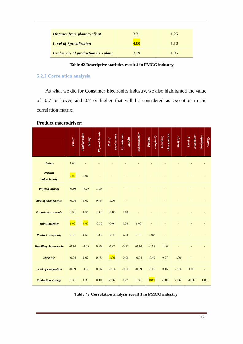
123

Distance from plant to client 3.31 1.25

Level of Specialization 4.00 1.10

Exclusivity of production in a plant 3.19 1.05



As what we did for Consumer Electronics industry, we also highlighted the value

of -0.7 or lower, and 0.7 or higher that will be considered as exception in the

correlation matrix.

Product macrodriver:

Vari

ety

Pro

du

ct v

alu

e

den

sity

Ph

ysic

al

den

sity

Ris

k o

f

obso

lesc

ence

Con

trib

uti

on

marg

in

Su

bst

itu

tabil

ity

Pro

du

ct

com

ple

xit

y

Han

dli

ng

chara

cter

isti

c

Sh

elf

life

Lev

el o

f

com

pet

itio

n

Pro

du

ctio

n

stra

tegy

Variety 1.00 - - - - - - - - - -

Product

value density 0.87 1.00 - - - - - - - - -

Physical density -0.36 -0.20 1.00 - - - - - - - -

Risk of obsolescence -0.04 0.02 0.45 1.00 - - - - - - -

Contribution margin 0.38 0.55 -0.08 -0.06 1.00 - - - - - -

Substitutability 1.00 0.87 -0.36 -0.04 0.38 1.00 - - - - -

Product complexity 0.48 0.55 -0.03 -0.49 0.33 0.48 1.00 - - - -

Handling charactristic -0.14 -0.05 0.20 0.27 -0.27 -0.14 -0.12 1.00 - - -

Shelf life -0.04 0.02 0.45 1.00 -0.06 -0.04 -0.49 0.27 1.00 - -

Level of competition -0.59 -0.61 0.36 -0.14 -0.61 -0.59 -0.10 0.16 -0.14 1.00 -

Production strategy 0.39 0.37 0.10 -0.37 0.27 0.39 0.89 -0.02 -0.37 -0.06 1.00

Table 43 Correlation analysis result 1 in FMCG industry

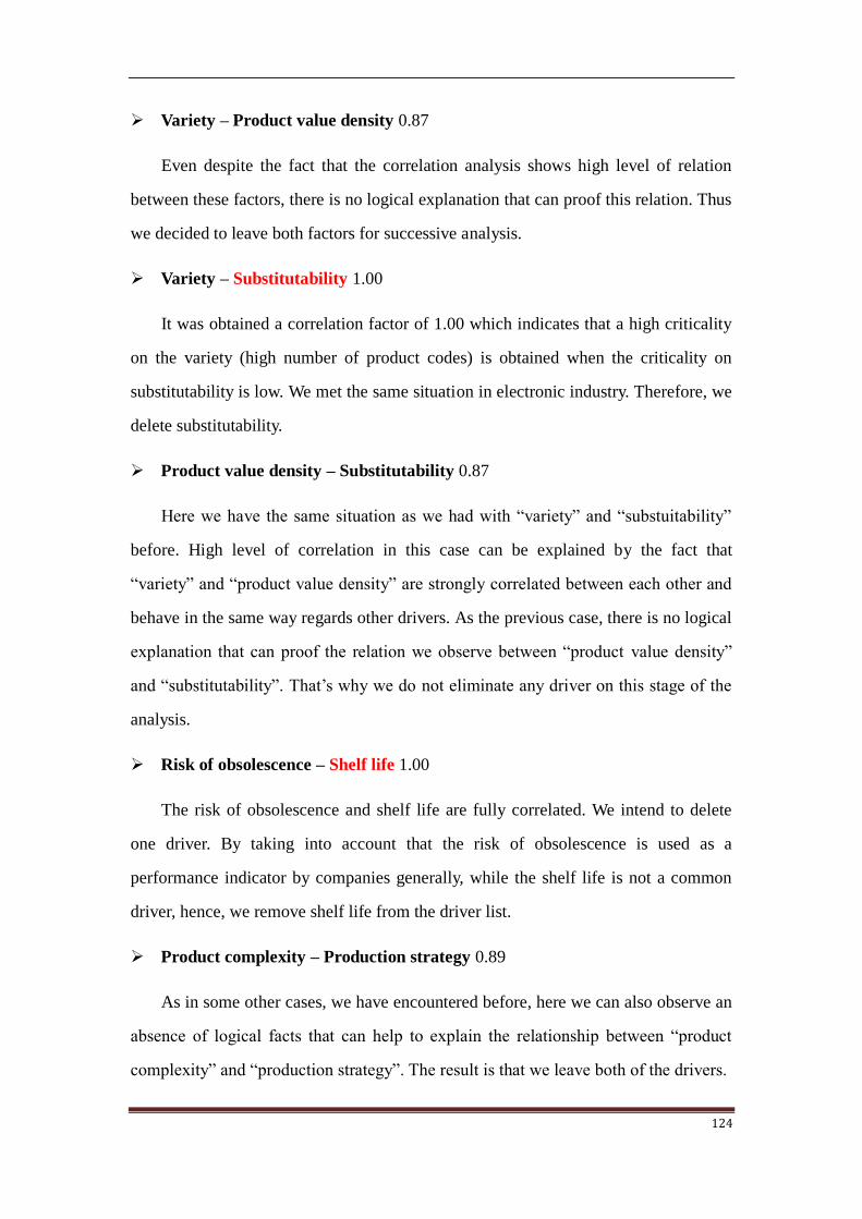
124

Variety – Product value density 0.87

Even despite the fact that the correlation analysis shows high level of relation

between these factors, there is no logical explanation that can proof this relation. Thus

we decided to leave both factors for successive analysis.

Variety – Substitutability 1.00

It was obtained a correlation factor of 1.00 which indicates that a high criticality

on the variety (high number of product codes) is obtained when the criticality on

substitutability is low. We met the same situation in electronic industry. Therefore, we

delete substitutability.

Product value density – Substitutability 0.87

Here we have the same situation as we had with “variety” and “substuitability”

before. High level of correlation in this case can be explained by the fact that

“variety” and “product value density” are strongly correlated between each other and

behave in the same way regards other drivers. As the previous case, there is no logical

explanation that can proof the relation we observe between “product value density”

and “substitutability”. That‟s why we do not eliminate any driver on this stage of the

analysis.

Risk of obsolescence – Shelf life 1.00

The risk of obsolescence and shelf life are fully correlated. We intend to delete

one driver. By taking into account that the risk of obsolescence is used as a

performance indicator by companies generally, while the shelf life is not a common

driver, hence, we remove shelf life from the driver list.

Product complexity – Production strategy 0.89

As in some other cases, we have encountered before, here we can also observe an

absence of logical facts that can help to explain the relationship between “product

complexity” and “production strategy”. The result is that we leave both of the drivers.

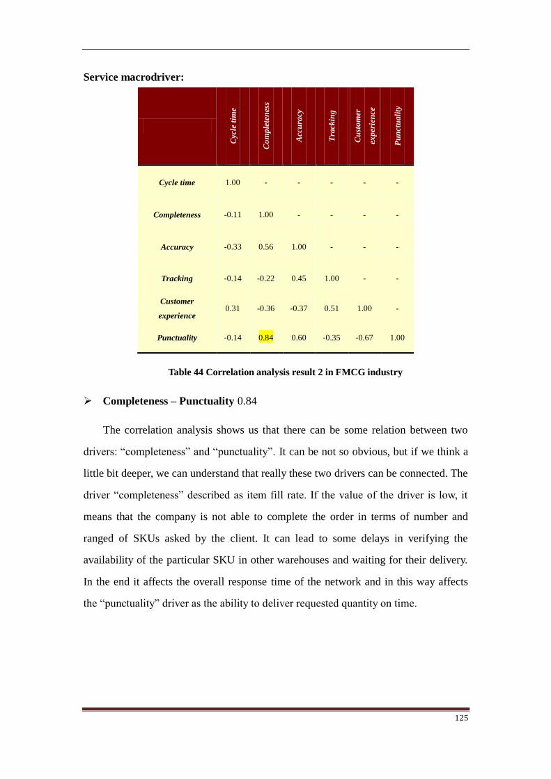
125

Service macrodriver:

Cyc

le t

ime

Co

mp

lete

nes

s

Acc

ura

cy

Tra

ckin

g

Cu

sto

mer

exp

erie

nce

Pu

nct

uali

ty

Cycle time 1.00 - - - - -

Completeness -0.11 1.00 - - - -

Accuracy -0.33 0.56 1.00 - - -

Tracking -0.14 -0.22 0.45 1.00 - -

Customer

experience 0.31 -0.36 -0.37 0.51 1.00 -

Punctuality -0.14 0.84 0.60 -0.35 -0.67 1.00


Completeness – Punctuality 0.84

The correlation analysis shows us that there can be some relation between two

drivers: “completeness” and “punctuality”. It can be not so obvious, but if we think a

little bit deeper, we can understand that really these two drivers can be connected. The

driver “completeness” described as item fill rate. If the value of the driver is low, it

means that the company is not able to complete the order in terms of number and

ranged of SKUs asked by the client. It can lead to some delays in verifying the

availability of the particular SKU in other warehouses and waiting for their delivery.

In the end it affects the overall response time of the network and in this way affects

the “punctuality” driver as the ability to deliver requested quantity on time.

126

Demand macrodriver:

Dim

ensi

on

of

the

ord

ers

Nu

mb

er

of

cust

om

ers

Del

iver

y

freq

uen

cy

Sea

son

ali

ty

Pre

dic

tab

ilit

y

of

dem

an

d

Sp

ati

al

den

sity

Dimension

of the orders 1.00 - - - - -

Number of

customers 0.15 1.00 - - - -

Delivery

frequency -0.43 -0.63 1.00 - - -

Seasonality -0.41 -0.11 0.26 1.00 - -

Predictability

of demand 0.39 0.44 -0.53 -0.36 1.00 -

Spatial

density -0.50 0.27 -0.44 0.27 -0.11 1.00


Supply macrodriver:

Nu

mb

er o

f p

lan

ts

Dis

tan

ce f

rom

pla

nt

to c

lien

t

Lev

el o

f

spec

iali

zati

on

Ex

clu

sivi

ty o

f

pro

du

ctio

n i

n a

pla

nt

Number of plants 1.00 - - -

Distance from

plant to client

0.49 1.00 - -

Level of specialization -0.07 0.54 1.00 -

Exclusivity of

production in a plant

0.40 0.61 0.81 1.00


Level of specialization – Exclusivity of production in a plant 0.81

As these two drivers can be seen as somehow similar one to another, we decide to

leave just one of them to reduce the complexity of the further analysis.

127

The result of available drivers in FMCG industry

Product

Variety

Physical Value Density

Physical Density

Risk of Obsolescence

Contribution Margin

Product Complexity


Level of Competition

Production Strategy

Service

Cycle Time

Completeness

Accuracy

Tracking

Customer Experience

Punctuality

Demand

Dimension of the order

Number of Customer

Delivery Frequency

Seasonality

Predictability of Demand

Spatial Density

Supply

Number of Plants



Total: 24

Table 47 Driver list after correlation analysis in FMCG industry

128


Theoretical Model

We assume that four factors are mutual independent. The following diagrams

represent the construct of each factor.

Graph 2 Theoretical model of CFA in FMCG industry

Product

vari

ety

pvd

ph

y_d

ens

risk

_ob

so

con

_mar

g

han

dlin

g

pro

_co

m

pro

d_s

tra

levl

_co

mp

Service

cyc_

tim

e

cus_

exp

e

trac

kin

g

accu

racy

com

ple

pu

nct

Demand

dim

_ord

nu

m_c

us

del

_fre

seas

on

pre

_dem

d

spa_

den

s

Support

nu

m_p

la

dis

t_p

tc

excl

_pro

d

129

Hypotheses

In the previous introduction, we have known the implication of the attributes and

the relation of these variables with different factors as the theoretical model we

showed. In the following discussion, we need to make hypotheses for every variable

in order to test if they really are important to the factor.

Product Factor:

Variety. The variety of products has direct impact on the stock cost and maintenance

cost for the total logistics costs. Therefore, H1P based on this influence.

H1P. Variety is positively related to product factor.

Physical value density. High value density products bring higher storage and lower

transport costs. On the other hand, the low value density products have opposite

impact on the storage and transport costs.

H2P. Physical value density is positively related to product factor.

Physical density. The physical density could influence both storage and


H3P. Physical density is positively related to product factor.

Risk of obsolescence. The length of life cycle tends to impact the inventory and

transportation costs in the logistics management.

H4P. Risk of obsolescence is positively related to product factor.

Contribution margin. The contribution margin is corresponding to transport policy

in logistics management, and hence impacts on the transportation costs.

H5P. Contribution margin is positively related to product factor.

Product complexity. Product complexity is related to the centralization of

distribution channel, and hence influences the total logistics costs.

H6P. Product complexity is positively related to product factor.

130

Handling characteristic. Differences in handling characteristic of products can

impact on distribution network costs and, therefore the most appropriate distribution

network selection should be done.

H7P. Handling characteristic is positively related to product factor.

Level of competition. Level of competition may bring the high inventory cost in

order to reduce the probability of stock out.

H8P. Level of competition is positively related to product factor.

Production strategy. Production strategy has impact on the inventory cost and

transport cost.

H9P. Production strategy is positively related to product factor.

Service Factor:

Cycle time. Cycle time could influence the number of facility and transportation

costs.

H1S. Cycle time is positively related to service factor.

Completeness. An increase in the required completeness will bring additional

inventory cost, but increase the service level.

H2S. Completeness is positively related to service factor.

Accuracy. Accuracy influences the transportation cost and inventory cost.

H3S. Accuracy is positively related to service factor.

Tracking. This attribute has different level of impact on different industries. The

direct influence on the logistics costs is the information cost.

H4S. Tracking is positively related to service factor.

Customer experience. Customer experience is influenced by the way of customers

purchase the product and the number of sales points. Hence, this variable has impact

131

on the facility cost and the lost of stock out.

H5S. Customer experience is positively related to service factor.

Punctuality. Punctuality influences the transportation cost and inventory cost.

H6S. Punctuality is positively related to service factor.

Demand Factor:

Dimension of the order. Dimension of the order which is determined by customer‟s

demand requirement has impact on transport cost.

H1D. Dimension of the order is positively related to demand factor.

Number of customers. The number of customers has significant impact on the

transportation cost due to the number of deliveries is caused by this attribute.

H2D. Number of customers is positively related to demand factor.

Delivery frequency. Delivery frequency influences the stock and maintenance costs,

which affects the different total logistics costs.

H3D. Delivery frequency is positively related to demand factor.

Seasonality. Seasonality affects stocking cost by increasing its levels in the seasons

it occurs, also increases the information requirements and the need of flexibility in

order to cope with the demand variations in those periods.

H4D. Seasonality is positively related to demand factor.

Predictability of demand. Predictability of demand has direct impact on the

inventory cost in order to cover the error in the demand forecast.

H5D. Predictability of demand is positively related to demand factor.

Spatial density. Spatial density mainly has impact on local transportation cost.

H6D. Spatial density is positively related to demand factor.

132

Supply Factor:

Number of plants. Number of plants has significant impact on the facility cost, and

influences the transportation cost as well.

H1Su. Number of plants is positively related to supply factor.

Distance from plant to client. The distance from plant to client affects total logistics


H2Su. Distance from plant to client is positively related to supply factor.

Exclusivity of production in a plant. Exclusivity of production in a plant is adverse

to level of specialization, while also has impact on the inventory cost and

transportation cost.

H3Su. Exclusivity of production in a plant is positively related to supply factor.

Hypotheses

Product Factor

1 Variety is positively related to product factor.

2 PVD is positively related to product factor.

3 Physical density is positively related to product factor.

4 Risk of obsolescence is positively related to product factor.

5 Contribution margin is positively related to product factor.

6 Product complexity is positively related to product factor.

7 Handling characteristic is positively related to product factor.

8 Level of competition is positively related to product factor.

9 Production strategy is positively related to product factor.

Service Factor

1 Cycle time is positively related to service factor.

2 Completeness is positively related to service factor.

3 Accuracy is positively related to service factor.

133

4 Tracking is positively related to service factor.

5 Customer experience is positively related to service factor.

6 Punctuality is positively related to service factor.

Demand Factor

1 Dimension of the order is positively related to demand factor.

2 Number of customers is positively related to demand factor.

3 Delivery frequency is positively related to demand factor.

4 Seasonality is positively related to demand factor.

5 Predictability of demand is positively related to demand factor.

6 Spatial density is positively related to demand factor.

Supply Factor

1 Number of plants is positively related to supply factor.

2 Distance from plant to client is positively related to supply factor.

3 Exclusivity of production in a plant is positively related to supply factor.

Table 48 Hypotheses for CFA in FMCG industry

Measurement model results

Product Factor:

The initial fit indices for product factor (e.g. P-value=0.963) suggests that

improvement could be made in the measures.

After the refinement, the re-specified measurement model for product factor

indicates an acceptable fit CFI=0.98, NNFI=0.97, RMSEA=0.008, /df=1.175,

P-value<0.1.

134

The first run:

CFI NNFI RMSEA /df

N/A N/A 0.000 0.57

Table 49 Initial result of CFA for product factor in FMCG industry

After improvement:


Physical density low loading(0.23) drop

Contribution margin low loading(0.49) drop

Handling characteristic low loading(0.08) drop

135

CFI NNFI RMSEA /df

0.98 0.97 0.008 1.175

Table 50 Final result of CFA for product factor in FMCG industry

Service Factor:

The initial fit indices for service factor (e.g. RMSEA=0.878, P-value=0.543)

suggest that improvement could be made in the measures.

After the improvement operation, the re-specified measurement model for

product factor indicates an acceptable fit CFI=0.91, NNFI=0.72, RMSEA=0.002,

/df=3.42, P-value=0.003

136

The first run:

CFI NNFI RMSEA /df

0.82 0.70 0.878 1.778

Table 51 Initial result of CFA for service factor in FMCG industry

After improvement:


Cycle time low loading(0.18) drop

Tracking low loading(0.26) drop

CFI NNFI RMSEA /df

0.91 0.72 0.002 3.42

Table 52 Final result of CFA for service factor in FMCG industry

137

Demand Factor

From the following diagram, we can see that the first fit indices for demand

factor (e.g. CFI=0.59, NNFI=0.19) propose that refinement should be done in order to

obtain a better goodness of fit.

After the refinement, a good model‟s fit is generated: CFI=0.86, NNFI=0.88,

RMSEA=0.051, /df=1.05, P-value=0.017

The first run:

CFI NNFI RMSEA /df

0.59 0.19 0.334 2.672

Table 53 Initial result of CFA for demand factor in FMCG industry

After improvement:


Seasonality low loading(0.44) drop

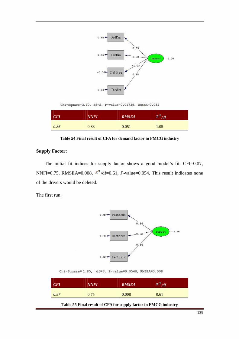
138

CFI NNFI RMSEA /df

0.86 0.88 0.051 1.05

Table 54 Final result of CFA for demand factor in FMCG industry

Supply Factor:

The initial fit indices for supply factor shows a good model‟s fit: CFI=0.87,

NNFI=0.75, RMSEA=0.008, /df=0.61, P-value=0.054. This result indicates none

of the drivers would be deleted.

The first run:

CFI NNFI RMSEA /df

0.87 0.75 0.008 0.61

Table 55 Final result of CFA for supply factor in FMCG industry

139

Finally, the results of measurement model show us a set of variables associated

four different factors in FMCG industry. These variables are selected by the factor

loading on the basis of covariance between the drivers and specific latent factor, and

the corresponding hypotheses are tested according to the statistics indicator.

Product

Variety


Risk of obsolescence

Product complexity


Production strategy

Service

Completeness

Accuracy

Customer experience

Punctuality

Demand


Number of customers

Delivery frequency

Predictability

Supply

Number of plants



Total: 17

Table 56 Driver list after CFA in FMCG industry

Hypotheses

Product

Factor

1 Variety is positively related to product factor. True

2 PVD is positively related to product factor. True

3 Physical density is positively related to product factor. False

140

4 Risk of obsolescence is positively related to product factor. True

5 Contribution margin is positively related to product factor. False

6 Product complexity is positively related to product factor. True

7 Handling characteristic is positively related to product factor. False

8 Level of competition is positively related to product factor. True

9 Production strategy is positively related to product factor. True

Service

Factor

1 Cycle time is positively related to service factor. False

2 Completeness is positively related to service factor. True

3 Accuracy is positively related to service factor. True

4 Tracking is positively related to service factor. False

5 Customer experience is positively related to service factor. True

6 Punctuality is positively related to service factor. True

Demand

Factor

1 Dimension of the order is positively related to demand factor. True

2 Number of customers is positively related to demand factor. True

3 Delivery frequency is positively related to demand factor. True

4 Seasonality is positively related to demand factor. False

5 Predictability of demand is positively related to demand factor. True

6 Spatial density is positively related to demand factor. False

Supply Factor

1 Number of plants is positively related to supply factor. True

2 Distance from plant to client is positively related to supply factor. True

3 Exclusivity of production in a plant is positively related to supply factor. True

Table 57 Hypotheses result of CFA in FMCG industry

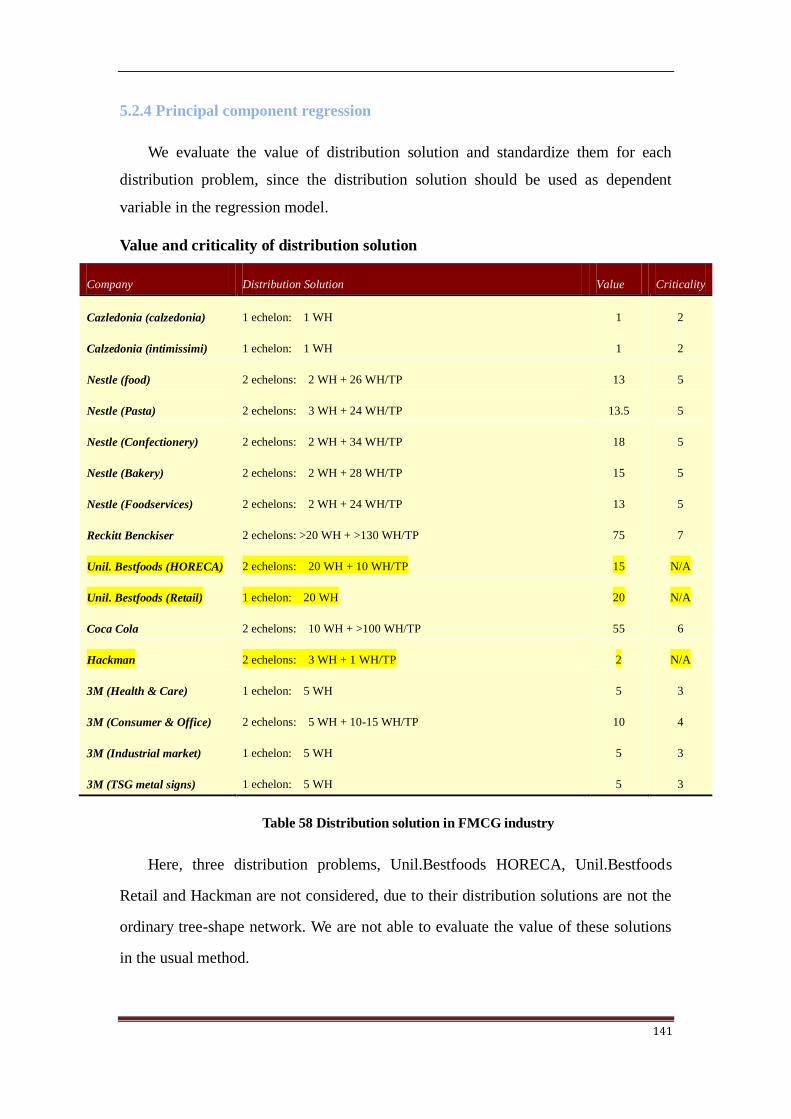
141


We evaluate the value of distribution solution and standardize them for each

distribution problem, since the distribution solution should be used as dependent

variable in the regression model.

Value and criticality of distribution solution

Company Distribution Solution Value Criticality

Cazledonia (calzedonia) 1 echelon: 1 WH 1 2

Calzedonia (intimissimi) 1 echelon: 1 WH 1 2

Nestle (food) 2 echelons: 2 WH + 26 WH/TP 13 5

Nestle (Pasta) 2 echelons: 3 WH + 24 WH/TP 13.5 5

Nestle (Confectionery) 2 echelons: 2 WH + 34 WH/TP 18 5

Nestle (Bakery) 2 echelons: 2 WH + 28 WH/TP 15 5

Nestle (Foodservices) 2 echelons: 2 WH + 24 WH/TP 13 5

Reckitt Benckiser 2 echelons: >20 WH + >130 WH/TP 75 7

Unil. Bestfoods (HORECA) 2 echelons: 20 WH + 10 WH/TP 15 N/A

Unil. Bestfoods (Retail) 1 echelon: 20 WH 20 N/A

Coca Cola 2 echelons: 10 WH + >100 WH/TP 55 6

Hackman 2 echelons: 3 WH + 1 WH/TP 2 N/A

3M (Health & Care) 1 echelon: 5 WH 5 3

3M (Consumer & Office) 2 echelons: 5 WH + 10-15 WH/TP 10 4

3M (Industrial market) 1 echelon: 5 WH 5 3

3M (TSG metal signs) 1 echelon: 5 WH 5 3

Table 58 Distribution solution in FMCG industry

Here, three distribution problems, Unil.Bestfoods HORECA, Unil.Bestfoods

Retail and Hackman are not considered, due to their distribution solutions are not the

ordinary tree-shape network. We are not able to evaluate the value of these solutions

in the usual method.

142

Regression Function

solutio=-14.0376+(-0.3636)variety+(-0.4481)pvd+(0.5065)riskobs+(0.218)complex+(-0.0971)compet+

(1.0615)prodstr+(1.2107)complet+(0.3362)accur+(1.9791)cusexpe+(-0.2913)punct+(-0.3766)dimord+(

0.1883)numcus+(0.0715)delfreq+(0.9039)predict+(-0.0919)numplan+(-0.0781)distptc+(-0.3961)exclu


2=0.990, F (11,1) =107.394, P=0.075

Driver Regression coefficient

Variety -0.3636


Risk of Obsolescence 0.5065


Level of Competition -0.0971

Product Strategy 1.0615

Completeness 1.2107

Accuracy 0.3362

Customer Experience 1.9791

Punctuality -0.2913

Dimension of the Order -03766

Number of Customers 0.1883



Number of Plants -0.0919

Distance from plant to client -0.0781


Table 59 Regression coefficient of drivers in FMCG industry

143

Chapter 6. Results

In this section, we will demonstrate the relationship between distribution

problem and distribution solution of the cases we investigated both in Consumer

Electronics industry and FMCG industry. As we introduced in the first chapter, the

theoretic model of distribution network selection matrix consists of four factors,

which could be divided into Firm and Market characteristics. In order to obtain the

final results, we figure out the value of these two characteristics and represent them in

a graphic illustration way.

6.1 Result of Consumer Electronics Industry

6.1.1 Analysis of four basic characteristics of distribution problem

First of all, as it is shown in the table provided below, we would like to analyze

the results we got for the Consumer Electronics Industry. For each of the distribution

problems that were described in details in the previous chapters, there are four

characteristics of product, service, demand and supply. Thereby, we should figure out

the values of these four characteristics of each distribution problem.

Distribution

problem

Product Service Demand Supply

HP 7.11 1.49 0.18 -0.38

SO1 7.99 -0.65 0.89 -1.10

SO2 7.99 0.07 2.04 -1.10

SO3 7.99 -1.37 3.19 -1.10

SO4 8.26 -0.65 0.70 -0.32

SO5 8.26 0.07 1.85 -0.32

SO6 8.26 -1.37 2.99 -0.32

SA1 6.18 0.53 1.08 -0.98

SA2 6.99 1.64 0.27 -0.98

SA3 6.99 3.08 0.98 -0.98

SA4 6.99 1.64 0.64 -1.49

SA5 6.99 3.08 1.26 -1.49

144

SA6 6.18 1.64 1.17 -0.90

SA7 6.18 3.08 1.79 -0.90

SA8 6.99 1.64 0.27 -0.98

SA9 6.99 3.08 0.98 -0.98

Table 60 Values of four basic characteristics in Consumer Electronics industry

6.1.2 Analysis of Firm and Market characteristics

As what we demonstrated in literature review, the theoretical model of existing

distribution network selection matrix could be described by the values of firm, market

and distribution solution. The values of firm and market of distribution problem are

the sum of product and supply factors, and the sum of service and demand factors as

the table shown above respectively. The value of the distribution solution is already

scaled and the meaning of the scale is given below:

1: direct shipment;



echelon and a few Warehouses/Transit Points (less than 15) in the 2nd

echelon;


echelon and several Warehouses/Transit Points (15 – 20) in the 2nd

echelon;



echelon;

Distribution

problem

Firm Market Distribution

solution

HP 6.75 1.68 2

SO1 6.90 0.24 2

145

SO2 6.90 2.11 3

SO3 6.90 1.81 3

SO4 7.96 0.05 2

SO5 7.96 1.92 4

SO6 7.96 1.62 4

SA1 5.20 1.61 1

SA2 6.01 1.91 2

SA3 6.01 4.06 4

SA4 5.51 2.28 2

SA5 5.51 4.34 4

SA6 5.28 2.81 2

SA7 5.28 4.87 5

SA8 6.01 1.91 2

SA9 6.01 4.06 4

Table 61 Result of Firm and Market characteristics in Consumer Electronics industry

6.1.3 Relationship between distribution problem and distribution solution

Now let‟s plot down the values we got on the chart (shown below). Each

distribution problem is marked with its own spot on the chart, has the name and the

value of distribution solution. For instance, SA1,1 means that we consider distribution

problem Samsung1 (SA1) and distribution solution for this problem is 1 (direct

shipment).

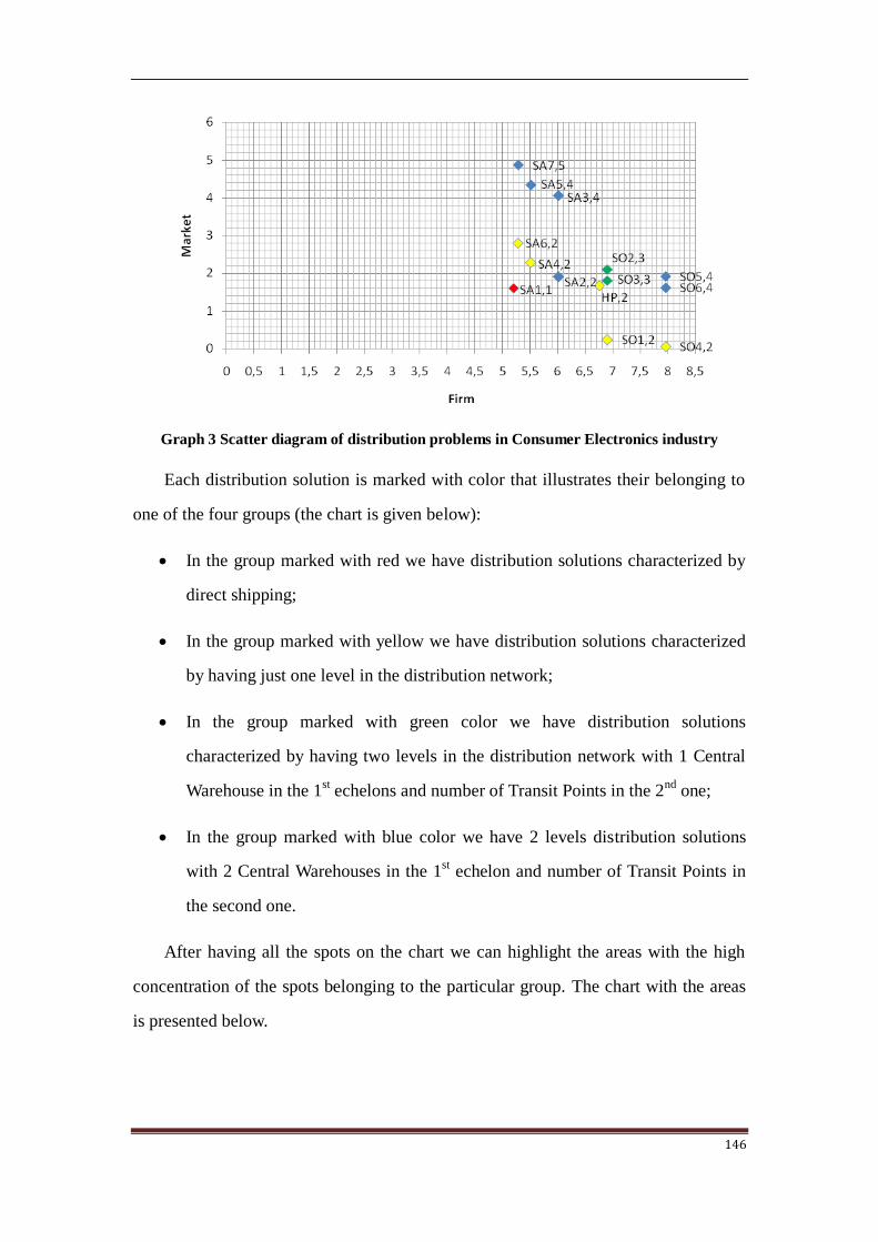
146

Graph 3 Scatter diagram of distribution problems in Consumer Electronics industry



In the group marked with red we have distribution solutions characterized by

direct shipping;




characterized by having two levels in the distribution network with 1 Central

Warehouse in the 1st echelons and number of Transit Points in the 2

nd one;


with 2 Central Warehouses in the 1st echelon and number of Transit Points in

the second one.

After having all the spots on the chart we can highlight the areas with the high

concentration of the spots belonging to the particular group. The chart with the areas

is presented below.

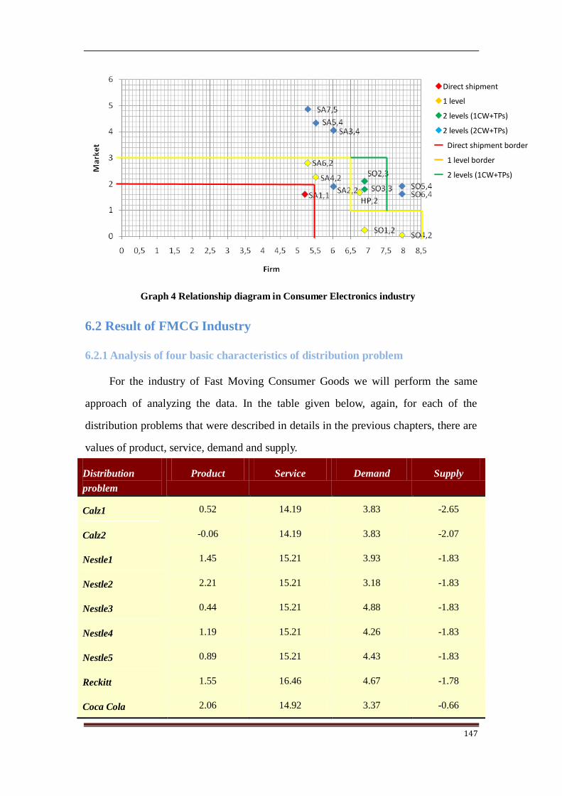
147

Graph 4 Relationship diagram in Consumer Electronics industry

6.2 Result of FMCG Industry

6.2.1 Analysis of four basic characteristics of distribution problem

For the industry of Fast Moving Consumer Goods we will perform the same

approach of analyzing the data. In the table given below, again, for each of the

distribution problems that were described in details in the previous chapters, there are

values of product, service, demand and supply.

Distribution

problem

Product Service Demand Supply

Calz1 0.52 14.19 3.83 -2.65

Calz2 -0.06 14.19 3.83 -2.07

Nestle1 1.45 15.21 3.93 -1.83

Nestle2 2.21 15.21 3.18 -1.83

Nestle3 0.44 15.21 4.88 -1.83

Nestle4 1.19 15.21 4.26 -1.83

Nestle5 0.89 15.21 4.43 -1.83

Reckitt 1.55 16.46 4.67 -1.78

Coca Cola 2.06 14.92 3.37 -0.66

◆Direct shipment

◆1 level



━ Direct shipment border

━ 1 level border

━ 2 levels (1CW+TPs)

border

148

3M1 2.22 14.20 3.24 -2.75

3M2 1.56 14.20 4.76 -2.75

3M3 1.65 14.20 3.74 -2.75

3M4 0.75 14.20 4.64 -2.75

Table 62 Values of basic characteristics in FMCG industry

6.2.2 Analysis of Firm and Market characteristics

According to the procedure we have done for Consumer Electronics industry

above, we can obtain the values of firm, market and distribution solution after the

analysis of four basic characteristics of distribution problem. The value of the

distribution solution is already scaled and the meaning of the scale is given below:

1: direct shipment;


3: 1 echelon with many Warehouses/Transit Points (more than 3);


echelon and a few Warehouses/Transit Points (up to 3) in the 2nd

one;



one;

6: 2 echelons with many Warehouses/Transit Points (more than 3) in the

1st echelon and a few Warehouses/Transit Points (up to 3) in the 2

nd one;

7: 2 echelons with many Warehouses/Transit Points (more than 3) in the

1st echelon and many Warehouses/Transit Points (more than 3) in the 2

nd

one.

Distribution

problem


solution

Calz1 -2.13 18.17 2

149

Calz2 -2.13 18.17 2

Nestle1 -0.39 19.42 5

Nestle2 0.37 18.67 5

Nestle3 -1.40 20.44 5

Nestle4 -0.65 19.68 5

Nestle5 -0.95 19.99 5

Reckitt -0.23 21.27 7

Coca Cola 1.40 18.64 6

3M1 -0.55 17.58 3

3M2 -1.20 19.24 4

3M3 -1.11 18.15 3

3M4 -2.01 19.05 3

Table 63 Result of Firm and Market characteristics in FNCG industry

On the above table, the value of Firm and Market is figured out by the drivers‟

coefficients. In order to compare the value of Firm and Market characteristics, a

coordinate transformation has to be carried out. A positive factor 3 and negative factor

17 are assigned to the value of Firm and Market respectively.

After the transformation:

Distribution

problem


solution

Calz1 0.87 1.17 2

Calz2 0.87 1.17 2

Nestle1 2.61 2.42 5

Nestle2 3.37 1.67 5

Nestle3 1.60 3.44 5

Nestle4 2.35 2.68 5

150

Nestle5 2.05 2.99 5

Reckitt 2.77 4.27 7

Coca Cola 4.40 1.64 6

3M1 2.45 0.58 3

3M2 1.80 2.24 4

3M3 1.89 1.15 3

3M4 0.99 2.05 3

Table 64 Result transformation in FMCG industry

6.2.3 Relationship between distribution problem and distribution solution

Again, like in the previous case, let‟s plot down the values we got on the chart

(shown below). Each distribution problem is marked with its own spot on the chart,

has the name and the value of distribution solution. For instance, Nestle3,5 means that

we consider distribution problem Nestle5 and distribution solution for this problem is

5 (two echelons with several WH/TP in the first echelon and many WH/TP in the

second one).

Graph 5 Scatter diagram of distribution problems in FMCG industry


151







nd one;




nd one;


with more than 5 Warehouses in the 1st

echelon and number of Transit Points in

the second one.

After having all the spots on the chart we can highlight the areas with the high

concentration of the spots belonging to the particular group. The chart with the areas

is presented below.

Graph 6 Relationship diagram in FMCG industry

152

Chapter 7. Conclusion

7.1 Comparison of drivers in different industries

In chapter 5, we have achieved 20 and 17 more important drivers for Consumer

Electronics industry and FMCG industry respectively after the application of

mathematical models. All of these drivers are able to reflect the product, service,

demand and supply features of a distribution problem. Some drivers could be used for

the two industries commonly, and several drivers have to be allocated to a kind of

industry especially due to the particular nature of an industry. Regarding the practical

application, we can use these drivers to evaluate the distribution problem in both

Consumer Electronics industry and FMCG industry.

Consumer Electronics Industry FMCG Industry

Product

Variety Variety

Product value density Product value density

Contribution margin Risk of obsolescence

Product complexity Product complexity

Level of competition Level of competition

ABC product characteristic Production strategy

Stage of life cycle

Service

Completeness Completeness

Accuracy & Punctuality Accuracy

Customer experience Customer experience

Cycle time Punctuality

Demand

Dimension of the orders Dimension of the orders

Delivery frequency Delivery frequency

Predictability of demand Predictability of demand

Demand volatility Number of customers

Demand level

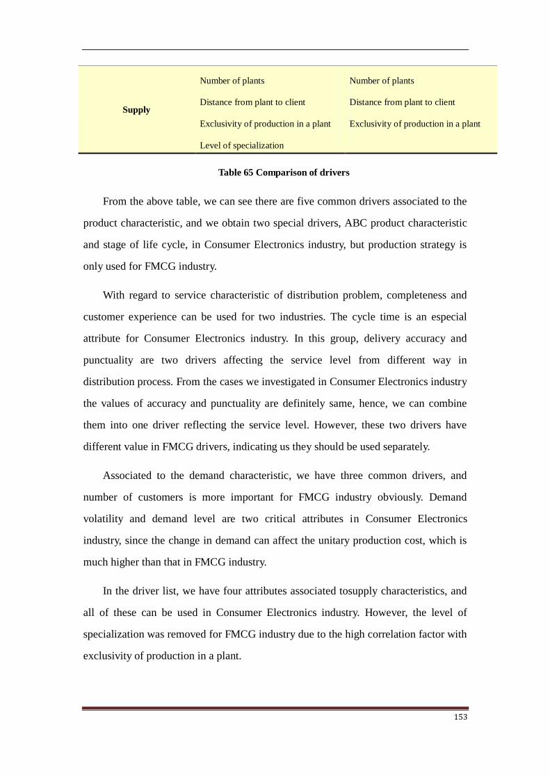
153

Supply

Number of plants Number of plants

Distance from plant to client Distance from plant to client

Exclusivity of production in a plant Exclusivity of production in a plant


Table 65 Comparison of drivers

From the above table, we can see there are five common drivers associated to the

product characteristic, and we obtain two special drivers, ABC product characteristic

and stage of life cycle, in Consumer Electronics industry, but production strategy is

only used for FMCG industry.

With regard to service characteristic of distribution problem, completeness and

customer experience can be used for two industries. The cycle time is an especial

attribute for Consumer Electronics industry. In this group, delivery accuracy and

punctuality are two drivers affecting the service level from different way in

distribution process. From the cases we investigated in Consumer Electronics industry

the values of accuracy and punctuality are definitely same, hence, we can combine

them into one driver reflecting the service level. However, these two drivers have

different value in FMCG drivers, indicating us they should be used separately.

Associated to the demand characteristic, we have three common drivers, and

number of customers is more important for FMCG industry obviously. Demand

volatility and demand level are two critical attributes in Consumer Electronics

industry, since the change in demand can affect the unitary production cost, which is

much higher than that in FMCG industry.

In the driver list, we have four attributes associated tosupply characteristics, and

all of these can be used in Consumer Electronics industry. However, the level of

specialization was removed for FMCG industry due to the high correlation factor with

exclusivity of production in a plant.

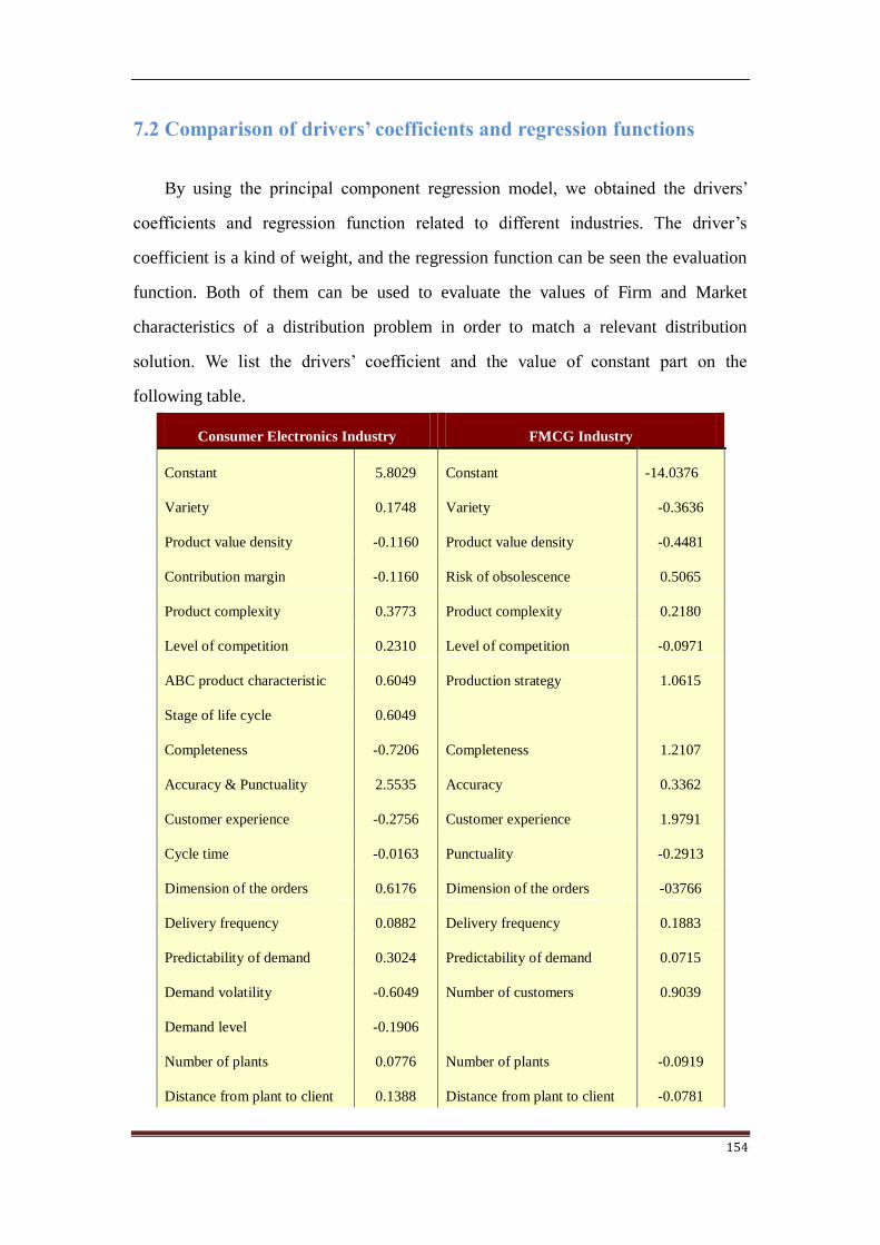
154

7.2 Comparison of drivers’ coefficients and regression functions

By using the principal component regression model, we obtained the drivers‟

coefficients and regression function related to different industries. The driver‟s

coefficient is a kind of weight, and the regression function can be seen the evaluation

function. Both of them can be used to evaluate the values of Firm and Market

characteristics of a distribution problem in order to match a relevant distribution

solution. We list the drivers‟ coefficient and the value of constant part on the

following table.


Constant 5.8029 Constant -14.0376

Variety 0.1748 Variety -0.3636

Product value density -0.1160 Product value density -0.4481

Contribution margin -0.1160 Risk of obsolescence 0.5065

Product complexity 0.3773 Product complexity 0.2180

Level of competition 0.2310 Level of competition -0.0971

ABC product characteristic 0.6049 Production strategy 1.0615

Stage of life cycle 0.6049

Completeness -0.7206 Completeness 1.2107

Accuracy & Punctuality 2.5535 Accuracy 0.3362

Customer experience -0.2756 Customer experience 1.9791

Cycle time -0.0163 Punctuality -0.2913

Dimension of the orders 0.6176 Dimension of the orders -03766

Delivery frequency 0.0882 Delivery frequency 0.1883

Predictability of demand 0.3024 Predictability of demand 0.0715

Demand volatility -0.6049 Number of customers 0.9039

Demand level -0.1906

Number of plants 0.0776 Number of plants -0.0919

Distance from plant to client 0.1388 Distance from plant to client -0.0781

155

Exclusivity of production in a

plant

-0.3341 Exclusivity of production in a

plant

-0.3961

Level of specialization -0.0795

Table 66 Comparison of drivers’ coefficients

The coefficients listed on the above table are not same in two industries even if

for the same driver since the different criticality value of this driver. However, the

results of goodness-of-fit are very good, the factor of each estimator indicate the

results of coefficients and the functions are believable and acceptable. We can see

them on the below table.


Adjusted R2 0.856 Adjusted R

2 0.990

F (10,5) 9.884 F (11,1) 107.394

P-value 0.010 P-value 0.075

Table 67 Result of goodness-of-fit for PCR

7.3 Comparison of normative selection matrixes

We have shown the distribution selection matrixes for both Consumer Electronics

industry and FMCG industry in the preceding chapter. The relationship between

distribution problem and distribution solution was represented in a graphic illustration.

We have known that the distribution network is more decentralized along with the

increase of the values of Firm and Market characteristics.

The following figures are the normative distribution network selection matrixes

in different industries.

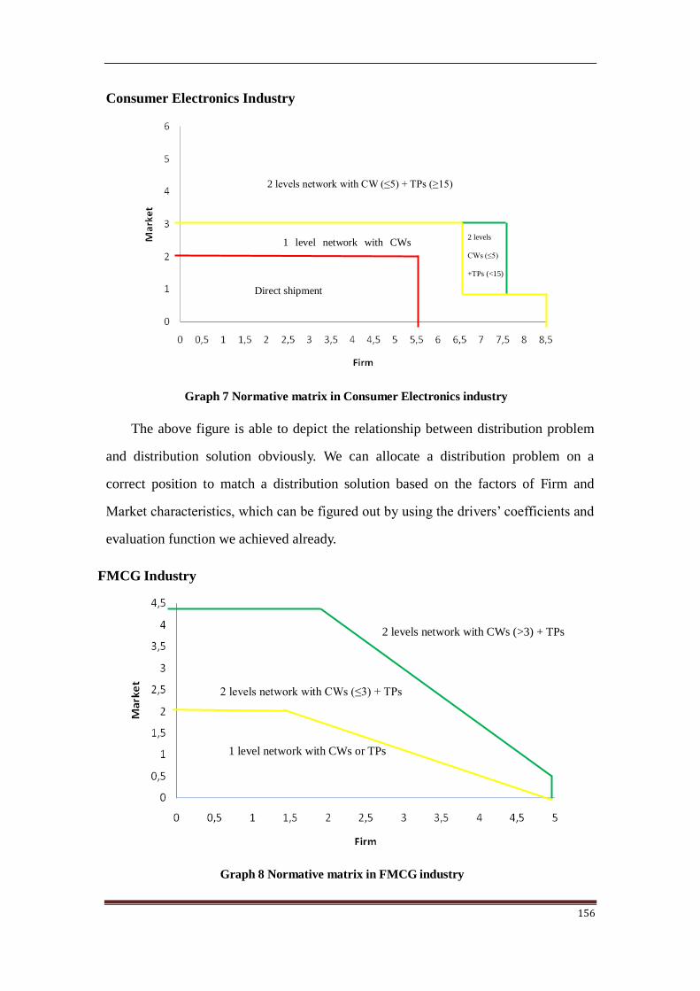
156

Consumer Electronics Industry

Graph 7 Normative matrix in Consumer Electronics industry

The above figure is able to depict the relationship between distribution problem

and distribution solution obviously. We can allocate a distribution problem on a

correct position to match a distribution solution based on the factors of Firm and

Market characteristics, which can be figured out by using the drivers‟ coefficients and

evaluation function we achieved already.

FMCG Industry

Graph 8 Normative matrix in FMCG industry

2 levels

CWs (≤5)

+TPs (<15)

Direct shipment

1 level network with CWs

(≤3)

2 levels network with CW (≤5) + TPs (≥15)

2 levels network with CWs (≤3) + TPs

1 level network with CWs or TPs

2 levels network with CWs (>3) + TPs

157

With regard to FMCG industry, we do not find any company adopts direct

shipment as distribution solution in the case study. This normative matrix is obtained

after the coordinate transformation we introduced in the previous chapter, hence, we

have to transform the factors of Firm and Market characteristics when we are figuring

out them by the drivers‟ coefficients and evaluation function.

7.4 Further development

We have used mathematical models to optimize the existing distribution network

selection matrixes for Consumer Electronics industry and FMCG industry. The

necessary important drivers‟ lists and related coefficients, evaluation functions have

been obtained. Finally, we achieved two normative distribution network selection

matrixes for the two industries. Therefore, based on the current results, we can

continue further development, for instance:

The sample size of both two industries in this study is 16, which is not large

enough. Hence, we may investigate more cases in order to enlarge the sample size

in order to make the quantitative analyses more accurate since the number of

samples can affect the accuracy of the statistical model.

This study is done based on Consumer Electronics industry and FMCG industry.

In fact, we can carry out the similar research for other more industries.

158

Bibliography:

A. Creazza and F. dallari, M. Melacini (2010), “Evaluating logistics network

configurations for a global supply chain”, Supply Chain Management : An

International Journal, 15/2, 154-164.

A.D.M.van de Ven, A.M.A. Ribers (1993), “International Logistics: A diagnostic

method for the allocation of production and distribution facilities”, The

International Journal of Logistics Management, Volume 4, Number 1.

Alan Rushton, and Richard Saw, “A methodology for logistics strategy planning”, The

International Journal of Logistics Management.

Alejandro Castro and Yamel Mattarollo (2010), Strategic Distribution Network

Design (DND) model and case studies in the Consumer Electronics Industry.

Antony Lovell, Richard Saw and Jennifer Stimson (2005), “Product value-density:

Managing diversity through supply chain segmentation”, The International

Journal of Logistics Management, Vol.16 No.1, pp142-158.

Archini, G., & Banno, M. (2003), Modelli di evoluzione dell’assetto dei sistemi

logistico produttivi di aziende multinazionali operanti du base europea.

Correlation Analysis, Direxionfunds, August 30, 2007.

C.S. Laluani, S.M. Disney and M.M. Naim (2006), “On assessing the sensitivity to

uncertain in distribution network design”, International Journal of Physical

Distribution & Logistics Management, Vol.36 No.1, pp 5-21.

Crosby, L. and LeMay, S.A. (1998), “Empirical determination of shipper requirements

for motor carrier services: SERVQUAL, direct questioning, and policy

capturing methods”, Journal of Business Logistics, Vol. 19 No. 1, pp. 139-53.

Daniela Ambrosino, Maria Grazia Scatella (2005), “Distribution Network Design:

New problems and related models”, European Journal of Operational

Research, 165(2005) 610-624.

Data Analysis, Texas State Auditor‟s Office, Methodology Manual, rev.5/1995.

Erik Selldin and Fan Olhager (2007), “Linking product with supply chains: testing

Fisher‟s model”, Supply Chain Management: An International Journal, 12/1,

42-51.

Euthemia Stavrulaki and Mark Davis (2010), “Aligning products with supply chain

processes and strategy”, The International Journal of Logistics Management,

Vol.21 No.1, pp 127-151.

Fari Collin, Eero Eloranta, Fan Holmstron (2009), “How to design the right supply

chain for your customer”, Supply Chain Management: An International

159

Journal, 14/6(2009) 411-417

Fontenot, G., Henke, L., Carson, K. and Philips, P. (2007), “Techniques for

determining importance: balancing scientific method and subjectivity”, Journal

of targeting, Measurement and Analysis for Marketing, Vol. 5 No.3, pp 170-80.

Gibson, B.J., Rutner, S.M. and Keller, S.B. (2002), “Shipper-carrier partnership issues,

rankings, and satisfaction”, International Journal of Physical Distribution &

Logistics Management, Vol.32 No.8, pp. 669-75.

Hau L.Lee (2004), “ The Triple-A Supply Chain”, Harvard Business Review.

H. Sharifi, H.S. Ismail and I. Reid (2006), “ Achieving agility in supply chain through

simultaneous „design of‟ and „design for‟ supply chain”, Journal of

Manufacturing Technology Management, Vol.17 No.8, pp1078-1098.

Introductory Statistics, 2nd Edition, Wiley. ISBN 0-471-31009-3, 1995.

Lin, J.R, & Lei, H.C (2009), “Distribution system design with two level routing

considerations”, Department of Transportation and Navigation Science,

National Taiwan Ocean University.

Luida K. Nozick, Mark A. Turnquist (2001), “Inventory, transportation, service

quality and the location of distribution centers”, Europe Journal of Operational

Research, 129(2001) 362-371.

Jack G.A.J van der Vorst, Stephan J. van Dijk and Adrie J.M. Beulens (2001), “Supply

chain design in the food industry”, The International Journal of Logistics

Management, Volume 12, Number 2.

J. Ben Naylor, Mohamed M Naim, Danny Berry (1999), “Leagility: Integrating the

lean and agile manufacturing paradigms in the total supply chain”,

International Journal of Production Economics, 62, 107-118.

Jon M. Sutter, John H. Kalivas, Patrick M. Lang (1992), “Which principal

components to utilize for principal component regression”, Journal of

Chemometrics, Volume 6, Issue 4, pages 217-225.

Joseph Sarkis (2003), “A strategic decision framework for green supply chain

management”, Journal of Cleaner Production，Volume 11, 397-409.

Jossef Perl, Sompong Sirisoponsilp (2007), “Distribution Networks: Facility Location,

Transportation and Inventory”, International Journal of Physical Distribution

& Logistics Management.

Marcel Mourits and Joseph J.M. Evers (1995), “Distribution Network Design: An

integrated planning support framework”, International Journal of Physical

Distribution & Logistics Management, Vol.25 No.5, pp43-57.

Marshall L. Fisher (1997), “What is the right supply chain for your product”, Harvard

http://en.wikipedia.org/wiki/Special:BookSources/0471310093

160

Business Review.

Martin Christopher, Denis Towill (2001), “An integrated model for the design of agile

supply chain”, International Journal of Physical Distribution and Logistics

Management, Vol.31, No.4, pp235-246.

Martin Christopher, Helen Peck, Denis Towill (2006), “A taxonomy for selecting

global supply chain strategies”, The International Journal of Logistics

Management, Vol.17 No.2, pp277-287.

Mery J. Meixell, Vidyaranya B. Gargeya (2005), “Global Supply Chain Design: A

literature review and critique”, Transportation Research Part E, 41(2005)

531-550.

Michael S. Garver and Zachary Williams, Stephen A. LeMay (2010), “Measuring the

importance of attributes in logistics research”, The International Journal of

Logistics Management, Vol.21 No.1, pp 22-44.

Min, H. and Lambert, T. (2002), “Truck driver shortage revisited”, Transportation

Journal, Vol. 42 No. 2, pp. 5-16.

Murphy, P.R. and Poist, R.F. (2000), “Third-party logistics: some user versus provider

perspective”, Journal of Business Logistics, Vol.21 No.1, pp. 29-36.

Paul Childerhouse, James Aitken, Denis R.Towill (2002), “Analysis and design of

focused demand chains”, Journal of Operation Management, 20, 675-689

P. Filzmoser. “Robust Pricipal Component Regression”, White Paper, Dept. of

statistics, Prob. Theory, and Actuarial Maths. Vienna University of Technology.

Qingyu Zhang, Mark A.Vonderembse and Jeen-Su Lim (2005), “Logistics flexibility

and its impact on customer satisfaction”, The International Journal of Logistics

Management, Vol. 16. No.1, pp.71-95

Rachel Mason-Jones, Ben Naylor, Denis R.Towill (2000), “Engineering the leagile

supply chain”, International Journal of Agile Management System, 2/1, 54-61.

Riccardo Manzini and Elisa Gebennini (2008), “Optimization models for the

dynamics facility location and allocation problem”, International Journal of

Production Research, Vol.46 No.8, 15 April 2008, 2061-2086.

Riccardo Manzini, Filippo bindi (2009), “Strategic design and operational

management optimization of a multi stage physical distribution system”,

Transportation Research Part E, 45(2009) 915-936.

Ronald H. Ballou (1993), “Reformulating a logistics strategy: A concern for the past,

present and future”, International Journal of Physical Distribution & Logistics

Management, Vol.23 No.5, pp30-38.

Ronald H. Ballou (1995), “Logistics Network Design: Modeling and informational

considerations”, The International Journal of Logistics Management, Volume 6,

161

Number 2.

Ronald H. Ballou (1999), Business Logistics Management, Fourth Edition.

Rushton, A., Oxley, J. and Crousher, P. (2000), Handbook of Logistics and

Distribution Management, Kogan Page, Longon.

Sunil Chopra (2003), “Designing the distribution network in a supply chain”,

Transportation Research Part E, 39(2003),123-140

Tim Payne, Melvyn J. Peters (2004), “What is the right supply chain for your

products”, The international Journal of Logistics Management, Volume 15,

Number 2.

Thomas Thron, Gabor Nagy and Niaz Wassan (2007), “Evaluating alternative supply

chain structures for perishable products”, The International Journal of

Logistics Management, Vol.18 No3, pp.364-384

Vaidyanathan Jayaraman (1998), “Transportation, facility location and inventory

issues in distribution network design-An investigation”, International Journal

of Operations & Production Management, Vol.18 No.5, pp 471-494.

Walid Klibi, Alain Martel, Adel Guitouni (2010), “The design of robust value-creating

supply chain networks: A critical review”, European Journal of Operational

Research, 203(2010) 283-293.

Wanke, P.F. and Zinn, W. (2004), “Strategic logistics decision making”, International

Journal of Physical Distribution & Logistics Management, Vol. 34 No. 6, pp.

466-78.

162

Appendix

Criticality value for Consumer Electronic industry

Product macrodriver

Va

riet

y

PV

D

Ph

ysic

al

Den

sity

Ris

k o

f O

bso

lesc

ence

Co

ntr

ibuti

on

Marg

in

Su

bst

itu

tabil

ity

Pro

duct

Com

ple

xity

Sta

ge

of

Lif

e C

ycle

Han

dli

ng

Cha

ract

eris

tic

Sh

elf

Lif

e

Valu

e

AB

C P

rod

uct

Cha

ract

eris

tic

Lev

el o

f C

om

pet

itio

n

Pro

duct

ion

Str

ate

gy

HP 5 5 5 4 2 1 5 4 2 2 3 3 4 3

SO1 2 1 3 3 1 2 4 4 2 4 4 4 5 4

SO2 2 1 3 3 1 2 4 4 2 4 4 4 5 4

SO3 2 1 3 3 1 2 4 4 2 4 4 4 5 4

SO4 4 4 2 2 2 2 5 4 2 1 3 4 5 4

SO5 4 4 2 2 2 2 5 4 2 1 3 4 5 4

SO6 4 4 2 2 2 2 5 4 2 1 3 4 5 4

SA1 1 5 1 5 4 5 5 4 2 5 3 3 4 4

SA2 1 1 4 1 3 5 5 5 2 2 2 3 4 4

SA3 1 1 4 1 3 5 5 5 2 2 2 3 4 4

SA4 3 3 3 3 2 3 5 4 2 5 4 3 4 4

SA5 3 3 3 3 2 3 5 4 2 5 4 3 4 4

SA6 1 5 1 5 4 5 5 4 2 5 1 3 4 4

SA7 1 5 1 5 4 5 5 4 2 5 1 3 4 4

SA8 1 2 3 1 2 4 5 5 2 2 5 3 4 4

SA9 1 2 3 1 2 4 5 5 2 2 5 3 4 4

163

Service macrodriver

Cyc

le T

ime

Co

mple

ten

ess

Ret

urn

ab

ilit

y

Acc

ura

cy

Tra

ckin

g

Cu

sto

mer

Exp

erie

nce

Pun

ctu

ali

ty

Abil

ity

to E

xped

ite

Ord

ers

HP 1 1 1 1 1 4 1 1

SO1 4 1 1 1 1 3 1 1

SO2 3 1 1 1 1 3 1 2

SO3 5 1 1 1 1 3 1 5

SO4 4 1 1 1 1 3 1 1

SO5 3 1 1 1 1 3 1 2

SO6 5 1 1 1 1 3 1 5

SA1 2 1 1 2 1 2 2 2

SA2 4 2 1 2 1 2 2 2

SA3 2 2 1 2 1 2 2 4

SA4 4 2 1 2 1 2 2 2

SA5 2 2 1 2 1 2 2 4

SA6 4 2 1 2 1 2 2 3

SA7 2 2 1 2 1 2 2 5

SA8 4 2 1 2 1 2 2 2

SA9 2 2 1 2 1 2 2 4

164

Demand macrodriver

Dim

esio

n o

f th

e

ord

er

Nu

mber

of

Cu

stom

er

Del

iver

y F

requ

ency

Sea

son

ali

ty

Pre

dic

tab

ilit

y o

f

Dem

and

Sp

ati

al

Den

sity

Dem

and

Vola

tili

ty

Dem

and

Lev

e

HP 1 2 5 2 3 3 3 3

SO1 1 2 4 3 5 4 2 1

SO2 3 2 3 3 5 4 2 1

SO3 5 5 2 3 5 1 2 1

SO4 1 2 4 2 5 4 2 3

SO5 3 2 3 2 5 4 2 3

SO6 5 5 2 2 5 1 2 3

SA1 4 1 1 5 3 5 3 3

SA2 3 3 1 1 3 4 3 5

SA3 4 4 2 1 3 3 3 5

SA4 3 2 3 3 3 4 3 3

SA5 4 4 3 3 3 3 3 3

SA6 4 2 2 5 3 4 3 2

SA7 5 4 2 5 3 3 3 2

SA8 3 3 1 1 3 4 3 5

SA9 4 4 2 1 3 3 3 5

165

Supply macrodriver

Nu

mb

er o

f P

lan

ts

Dis

tan

ce f

rom

pla

nt

to c

lien

t

Lev

el o

f

Sp

ecia

liza

tio

n

Exc

lusi

vity

of

pro

du

ctio

n i

n a

pla

nt

HP 4 4 3 3

SO1 3 2 5 1

SO2 3 2 5 1

SO3 3 2 5 1

SO4 4 5 3 4

SO5 4 5 3 4

SO6 4 5 3 4

SA1 2 5 5 2

SA2 1 5 5 1

SA3 1 5 5 1

SA4 1 2 5 4

SA5 1 2 5 4

SA6 2 5 5 1

SA7 2 5 5 1

SA8 1 5 5 1

SA9 1 5 5 1

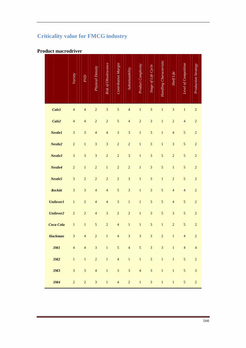
166

Criticality value for FMCG industry

Product macrodriver

Va

riet

y

PV

D

Ph

ysic

al

Den

sity

Ris

k o

f O

bso

lesc

ence

Co

ntr

ibuti

on

Marg

in

Su

bst

itu

tabil

ity

Pro

duct

Com

ple

xity

Sta

ge

of

Lif

e C

ycle

Han

dli

ng

Cha

ract

eris

tic

Sh

elf

Lif

e

Lev

el o

f C

om

pet

itio

n

Pro

duct

ion

Str

ate

gy

Calz1 4 4 2 3 5 4 1 3 1 3 1 2

Calz2 4 4 2 2 5 4 2 3 1 2 4 2

Nestle1 3 3 4 4 3 3 1 3 1 4 5 2

Nestle2 2 1 3 3 2 2 1 3 1 3 5 2

Nestle3 3 3 3 2 2 3 1 3 5 2 5 2

Nestle4 2 1 2 1 2 2 1 3 5 1 5 2

Nestle5 3 2 2 2 2 3 1 3 1 2 5 2

Reckitt 3 3 4 4 5 3 1 3 5 4 4 2

Unilever1 1 2 4 4 3 1 1 3 5 4 5 2

Unilever2 2 2 4 3 2 2 1 3 5 3 5 2

Coca Cola 1 1 5 2 4 1 1 3 1 2 5 2

Hackman 3 4 2 1 4 3 3 3 2 1 4 2

3M1 4 4 3 1 5 4 5 3 3 1 4 4

3M2 1 1 2 1 4 1 1 3 1 1 5 2

3M3 3 3 4 1 3 3 4 3 1 1 5 3

3M4 2 2 3 1 4 2 1 3 1 1 5 2

167

Service macrodriver

Cyc

le T

ime

Co

mple

ten

ess

Acc

ura

cy

Tra

ckin

g

Cu

sto

mer

Exp

erie

nce

Pun

ctu

ali

ty

Calz1 2 5 5 4 4 5

Calz2 2 5 5 4 4 5

Nestle1 1 4 4 5 5 3

Nestle2 1 4 4 5 5 3

Nestle3 1 4 4 5 5 3

Nestle4 5 4 4 5 5 3

Nestle5 3 4 4 5 5 3

Reckitt 2 5 5 5 5 4

Unilever1 1 4 3 5 5 3

Unilever2 2 4 3 5 5 3

Coca Cola 3 4 4 5 5 4

Hackman 1 4 4 4 3 4

3M1 3 4 1 4 5 3

3M2 3 4 1 4 5 3

3M3 3 4 1 4 5 3

3M4 3 4 1 4 5 3

168

Demand macrodriver

Dim

esio

n o

f th

e

ord

er

Nu

mber

of

Cu

stom

er

Del

iver

y F

requ

ency

Sea

son

ali

ty

Pre

dic

tab

ilit

y o

f

Dem

and

Sp

ati

al

Den

sity

Calz1 1 2 5 4 4 2

Calz2 1 2 5 5 4 2

Nestle1 3 4 1 1 5 3

Nestle2 5 4 1 1 5 3

Nestle3 1 5 2 5 5 5

Nestle4 2 3 2 5 5 3

Nestle5 2 5 1 1 5 4

Reckitt 1 2 4 1 5 2

Unilever1 2 4 2 4 5 3

Unilever2 5 2 2 1 5 2

Coca Cola 5 5 2 5 5 1

Hackman 3 1 3 5 5 2

3M1 2 2 2 5 4 5

3M2 1 4 2 5 5 5

3M3 1 3 2 5 4 5

3M4 1 3 2 5 5 5

169

Supply macrodriver

Nu

mb

er o

f P

lan

ts

Dis

tan

ce f

rom

pla

nt

to c

lien

t

Lev

el o

f

Sp

ecia

liza

tio

n

Exc

lusi

vity

of

pro

du

ctio

n i

n a

pla

nt

Calz1 3 5 5 5

Calz2 1 5 5 4

Nestle1 1 2 4 4

Nestle2 1 2 4 4

Nestle3 1 2 4 4

Nestle4 1 2 4 4

Nestle5 1 2 4 4

Reckitt 3 4 2 3

Unilever1 2 4 5 4

Unilever2 1 4 5 5

Coca Cola 2 1 1 1

Hackman 3 4 5 5

3M1 5 4 4 5

3M2 5 4 4 5

3M3 5 4 4 5

3M4 5 4 4 5

Documents

POLITECNICO DI MILANO · 2013-03-05 · POLITECNICO DI MILANO POLO REGIONALE DI COMO Master of Science in Management, Economics and Industrial Engineering Strategic Distribution Network