WP-2008-012

Policy Dilemmas in India: The Impact of Changes in Agricultural Prices on

Rural and Urban Poverty

Sandra Polaski, Manoj Panda, A. Ganesh-Kumar, Scott McDonald, and Sherman Robinson

Indira Gandhi Institute of Development Research, Mumbai June 2008

http://www.igidr.ac.in/pdf/publication/WP-2008-012.pdf

CORE Metadata, citation and similar papers at core.ac.uk

Provided by Research Papers in Economics

2

Policy Dilemmas in India: The Impact of Changes in Agricultural Prices on

Rural and Urban Poverty1

Sandra Polaski, Manoj Panda, A. Ganesh-Kumar, Scott McDonald, and Sherman Robinson2

Indira Gandhi Institute of Development Research (IGIDR)

General Arun Kumar Vaidya Marg Goregaon (E), Mumbai- 400065, INDIA

Abstract

Trade policy reforms which lead to changes in world prices of agricultural commodities or domestic policies aimed at affecting agricultural prices are often seen as causing a policy dilemma: a fall in agricultural prices benefits poor urban consumers but hurts poor rural producers, while a rise yields the converse. Poor countries have argued that they need to be able to use import protection and/or price support policies to protect themselves against volatility in world agricultural prices in order to dampen these effects. In this paper, we explore this dilemma in a CGE model of India that uses a new social accounting matrix (SAM) developed at the Indira Ghandi Institute of Development Research (IGIDR) in Mumbai. The SAM includes extensive disaggregation of agricultural activities, commodity markets, labor markets, and rural and urban households. This SAM includes 115 commodities, 48 labor types and 352 types of households, (classified by social group, income class, region, and urban/rural). The CGE model based on this SAM can be used to explore the linkages between changes in world prices of agriculture and the incomes of poor rural and urban households, capturing rural-urban linkages in both commodity and factor markets. The results indicate that the inclusion of linkages between rural and urban labor markets is necessary to fully explore, and potentially eliminate, the dilemma. A fall in agricultural prices hurts agricultural producers, lowers wages and/or employment of rural labor, and in some cases spills over into urban labor markets, depressing wages and incomes of poor urban households as well. In these cases both rural and urban poverty increases. The paper explores the strength of these commodity and factor market linkages, and the potential spillover effects of policies affecting agricultural prices. Key words: Doha negotiations, India trade policy, World prices, Labour market, CGE model JEL Codes: F13, F14, F16, O24, O53

1 This paper has been presented at the 11th Annual Conference on Global Economic Analysis organised by Purdue University and UN-WIDER, Helsinki, Finland, June 12-14, 2008. 2 Sandra Polaski, spolaski@carnegieendowment.org, is with Carnegie Endowment for International Peace, Manoj Panda, manon@igidr.ac.in and A. Ganesh-Kumar, agk@igidr.ac.in, are with IGIDR, Scott McDonald, s.mcdonald@sheffield.ac.uk, is with Oxford Brookes University and Sherman Robinson, sherman.robinson@sussex.ac.uk, is with the Institute of Development Studies (IDS), University of Sussex.

3

Policy Dilemmas in India: The Impact of Changes in Agricultural Prices on

Rural and Urban Poverty

Sandra Polaski, Manoj Panda, A. Ganesh-Kumar, Scott McDonald, and Sherman Robinson

1. Introduction and Motivation

India’s economic growth has accelerated in recent years, and its share of world trade

has expanded. Yet, despite these recent positive trends, India remains the largest reservoir of

poverty in the world (Figure 1). Its recent high growth has been driven mainly by its modern

services sector, which accounts for only a small proportion of overall employment and

household incomes. Its agricultural sector, where poverty is concentrated, is in a deep crisis.

The country faces daunting challenges and policy decisions to create employment for its

burgeoning population and raise incomes across the full range of households, skill levels,

sectors, and regions.

India’s bound tariffs are still relatively high, although applied tariffs are much lower.

Because of this gap, the government currently retains significant policy space with respect to

trade and agricultural prices, including the ability to raise and lower tariffs in response to

world price changes and prevailing conditions. In the Doha Development Agenda round of

negotiations at the World Trade Organization, the Indian government has sought to maintain

its policy space with respect to agricultural prices. Specifically, it has sought provisions in

the Doha round to treat some agricultural commodities as “special products” that would be

subjected to lesser or no tariff cuts based on considerations such as livelihood security. It

4

also seeks a “special safeguard mechanism” through which it would retain the ability to raise

tariffs in response to agricultural price drops or import surges.3

The question of the impact of trade liberalization on poverty has long concerned both

policy makers and the research community; however there has been limited research that

illuminates the causal relationships. Most ex post studies of the relationship between changes

in trade and changes in income levels and distribution (sometimes explicitly including

poverty) have tended to focus on the manufacturing sector and urban areas. Since most of the

world’s poor are in rural areas and more are engaged in agriculture than in manufacturing,

this body of literature has limited usefulness with respect to poverty implications. A few

recent studies that probe the relationship between trade liberalization, including the

agricultural sector, and poverty are discussed in Section 5, below.

We use a computable general equilibrium model of the Indian economy to explore the

impact on Indian households and poverty of changes in global prices for rice and wheat,

which are the most important food grains in India. Global price changes would have a

stronger impact on the country’s producers and consumers if the government were to lower

and bind its agricultural tariffs as a result of the Doha round. We trace the impact of global

price volatility on the overall economy, factors of production, and households. Using a new

social accounting matrix (SAM) for India, we are able to capture the impacts on highly

disaggregated types of labor and households, including information on social groups (castes,

tribes, etc.), income levels and location. We believe that this is the first study that looks at

3 India’s position is supported by a coalition of developing countries known as the G33. The G33 includes the following 46 countries: Antigua and Barbuda, Barbados, Belize, Benin, Bolivia, Botswana, China, Congo, Côte d’Ivoire, Cuba, Dominica, Dominican Republic, El Salvador, Grenada, Guatemala, Guyana, Haiti, Honduras, India, Indonesia, Jamaica, Kenya, Rep. Korea, Madagascar, Mauritius, Mongolia, Mozambique, Nicaragua, Nigeria, Pakistan, Panama, Peru, Philippines, St Kitts and Nevis, St Lucia, St Vincent and the Grenadines, Senegal, Sri Lanka, Suriname, Tanzania, Trinidad and Tobago, Turkey, Uganda, Venezuela, Zambia, Zimbabwe (World Trade Organization, 2007a).

5

the impact of global agricultural price changes—and therefore the potential impact of trade

policy change—on poverty at such a detailed and disaggregated level.

The study is organized as follows. Section 2 puts the present study in context by

providing an overview of Indian poverty, agriculture, employment, and trade. The following

section describes the analytical framework of the study. Section 4 presents the results. As

noted, Section 5 briefly reviews the results from several recent studies that attempt to assess

the impact of trade on poverty in India or globally. A final section suggests policy

implications of the findings and concludes.

2. The Context: Indian Poverty, Agriculture, Employment, and Trade

Although India’s aggregate economy is large, when divided by its 1.1 billion people,

the resulting per capita income places it in the ranks of low-income countries. Its GDP per

capita stood at $785 in the most recent measure by the International Monetary Fund, ranking

it 134th of 185 member countries (International Monetary Fund 2007b). Using the traditional

purchasing power parity (PPP) conversion, its GDP per capita stands at about $3,800, similar

to the levels of Nicaragua, Angola, and Vietnam. Using newly revised World Bank and Asian

Development Bank estimates, GDP per capita is significantly smaller, at about $2,100 (Asian

Development Bank 2007).

The vast majority of the population suffers from very low incomes (Figure 1). The

new PPP estimates suggest that 792 million people, or 73 percent of the population, live on

less than $1 per day, while slightly over a billion people, or 94 percent of the population, live

on less than $2 per day.4 As measured by the national poverty line, the percentage of the

population living below the poverty line has fallen in recent years; however due to population

4 Authors’ calculations using the World Bank’s PovcalNet software, http://iresearch.worldbank.org/PovcalNet.

6

growth, the number of poor people has barely decreased. In 2004–2005, 77 percent of the

population, totaling 836 million people, had an income below 20 rupees per day (twice the

official poverty line), which is approximately 50 cents at the current exchange rate (NCEUS

2007).

Poverty in India is concentrated in rural areas, as it is in most of the developing world.

Nearly three-quarters of India’s poor live in the countryside, where the proportion of the

population living at or below the national poverty line is 28.3 percent, compared with 25.7

percent in urban areas (National Sample Survey Organisation 2005). This is driven in large

part by deeply rooted problems and slow growth in the agricultural sector, discussed below.

Indian poverty is also characterized by an element of ethnicity and caste. Historically,

disadvantaged castes, tribes, and some other classes suffered discrimination and exclusion

from many economic opportunities. The Indian Constitution recognizes the groups that have

been disadvantaged and the government has accorded compensatory advantages to try to

redress the effects. The Constitution and laws establish specific opportunities for groups

officially identified as “scheduled tribes” (ST), “scheduled castes” (SC), and “other backward

classes” (OBC). Nonetheless, these groups continue to suffer considerably higher levels of

poverty and more exclusion than other groups. In the government’s 1999–2000 survey, the

proportions of people below the official poverty line were 45.8 percent for “scheduled

tribes,” 35.9 percent for “scheduled castes,” and 27 percent for “other backward classes,”

compared with 15 percent for the rest of the population (Panda (2007a).

Poverty is accompanied by widespread child malnutrition. According to a UNICEF

study (2006), 47 percent of children under the age of five years were underweight, among the

highest rates in the world (Bangladesh and Nepal have rates of 48 percent). In absolute

numbers, India has 57 million underweight young children, the largest concentration in the

world. Malnutrition at such levels is a humanitarian tragedy. In economic terms, it also has

7

dire consequences for the country’s future, because it is likely to constrain growth and

productivity for the foreseeable future. Malnourished children are more likely to die, to suffer

recurring illness later in life, and to have learning impairment. What happens to Indian

children today will affect the economy for the next six decades.

India produces about 210 million tons of food grains, mainly rice and wheat, which

make up the staple food supply of the country. It was a large importer of food grains until the

mid-1970s, but it has been self-sufficient and even a net exporter in most years during the last

two decades. This turnaround was the result of the adoption of high-yielding varieties of

seeds and chemical fertilizers, along with large public investments in irrigation. These

measures made up what has come to be called the “green revolution” and also involved

government procurement operations and guaranteed minimum support prices to farmers for

food grains in some parts of the country. The increase in agricultural output since 1980–1981

has been mostly due to a rise in yield per hectare attributable to the green revolution, rather

than expansion of total area under cultivation.

India has the second-largest potential labor force in the world, after China (ILO

2007). However participation rates are relatively low and unemployment is high. The labor

force participation rate was highest among “scheduled tribes” (51 percent), followed by

“scheduled castes” (44 percent) and “other backward classes” (43 percent). For other groups,

the participation rate was 40 percent.

About 55 percent of the workforce continues to depend on agriculture as the main

source of livelihood, although it contributes only 19 percent to overall GDP. The income of a

typical worker in agriculture is one-fifth of a counterpart in nonagricultural sectors. The bulk

of the rural poor consists of landless laborers and marginal farmers owning less than one

hectare of land. The proportion of rural male workers engaged in the agricultural activities

declined gradually from 81 percent in 1977–1978 to 67 percent in 2004–2005, whereas for

8

rural female workers, the decline was less, from 88 percent in 1977–1978 to 83 percent in

2004–2005.

Among urban workers, the largest source of employment for males was the “trade,

hotel, and restaurant” sectoral grouping, which employed 28 percent of urban male workers,

followed by manufacturing at 24 percent and “other services” at 21 percent. Between the

1999–2000 and 2004–2005 surveys, the proportion of urban females employed in the

manufacturing sector increased from 24 to 28 percent, while the share employed in the trade,

hotel, and restaurant sector fell by 5 percent.

According to projections prepared by the Government of India’s Planning

Commission (2004), India’s labor force is expected to increase by about 160–170 million by

2020, a growth of about 2 percent a year. The report estimates that to absorb this growing

workforce as well as to offer employment to the 35 million persons unemployed or

underemployed as of 2002, the country will need to generate about 200 million additional

employment opportunities by 2020.

Trade policy changes can have important effects on poverty—both positive, through

improvements in export opportunities or lower prices, for example, and negative, if cheaper

imports reduce the incomes of poor farmers or eliminate employment opportunities in some

sectors without creating sufficient jobs in others. The country remains one of the less open

economies among large developing countries, with average applied tariffs of 12.1 percent

(14.1 percent including ad valorem equivalents) on nonagricultural products and 40.8 percent

on agricultural products (World Trade Organization (2007c). Because such a high proportion

of India’s labor force is still engaged in agriculture, and the sector is still the main reservoir

of poverty in the country, liberalization of agricultural trade is likely to have a significant

impact on Indian poverty.

9

3. Analytical Framework

The model: The model of the Indian economy used in this study is the “STAGE”

(Static Applied General Equilibrium) model developed by Scott McDonald. It is a member of

the class of single-country CGE models that are descendants of the approach to CGE

modeling described by Dervis, de Melo, and Robinson (1982) and models reported by

Robinson, Kilkenny, and Hanson (1990) and Kilkenny (1991). The model is a social

accounting matrix–based CGE model, and the modeling approach has been influenced by

Pyatt’s “SAM Approach to Modeling” (Pyatt 1987). We vary the standard closure of full

employment of all labor with an alternative labor market closure meant to reflect

unemployment and underemployment among unskilled laborers in India. The results we

report are for this alternative. A short description of the model is presented in Appendix A.

The social accounting matrix: The social accounting matrix (SAM) used in this

study was constructed by Scott McDonald, Manoj Panda and A. Ganesh-Kumar. It improves

upon earlier SAMs for the Indian economy by incorporating detailed information on sources

of incomes at the household level. Previous SAMs included extensive information on

consumption expenditures but were less satisfactory regarding sources of household income.

The distribution of Indian households by income, location (rural or urban), and social

group as reflected in the model are presented in Tables 1 (countrywide distribution), 2 (rural

distribution), and 3 (urban distribution).

A description of the SAM is presented in Appendix B. Table B.1 presents the

macroeconomic totals for the SAM, while Table B.2 provides an overview of the Indian

economy as represented in the model.

The policy scenarios and simulations: We use the model to simulate the impact on

poverty and income distribution of changes in world agricultural prices for some key crops.

These changes could arise as the result of trade or agricultural policy changes elsewhere in

10

the world, behavior by private actors, weather, or other causes. They shed light on potential

effects of an agreement in the Doha round because such an agreement would require India (as

well as other countries) to bind its tariffs at lower levels. As a result, the government would

have less scope for raising tariffs to offset negative global price changes that could lower

domestic farm incomes, the source of livelihood for a majority of Indian households. On the

other hand, households would face lower prices as consumers of these key commodities,

which could offset the income effects.

Because of their concerns about the impact of negative price shocks, India and other

developing countries for which agriculture is a major source of employment and livelihoods

have proposed that they be allowed special treatment in the Doha round to address this

vulnerability. As noted above, a coalition known as the Group of Thirty-Three (G33), has

proposed that developing countries be allowed to shield a certain number of “special

products” from full tariff cuts because of their importance for livelihood security, food

security, or rural development. They have also proposed that a “special safeguard

mechanism” be created whereby they could temporarily raise tariffs to counter sharp changes

in the price or volume of imports that could threaten local livelihoods. Our simulation sheds

light on the need for such measures and their potential impact on poverty in India.

Specifically, we simulate the impact on the Indian economy of a 25 percent decrease,

a 50 percent decrease, a 25 percent increase, and a 50 percent increase in the world prices for

rice and wheat, which are the most important food grains in India in terms of production and

household consumption. These price changes would have stronger effects under a Doha

agreement compared to bilateral or regional free trade agreements because Indian tariffs

would be lowered toward all trading partners, including the lowest-cost producers. We use

the model to probe the differential effects on different types of labor and on households of

different social groups, at different income levels, and in rural and urban areas in order to

11

explore the consequences for income distribution and poverty. Although world prices may

not be transmitted perfectly to all households, price data for India show a considerable degree

of linkage with world prices for rice and wheat (Conforti 2004).5 In the case of rice, import

prices move with world prices and within the domestic market prices are transmitted fairly

completely between wholesale and retail and between producer and export prices.

Global agricultural price swings of this magnitude are not uncommon, as seen in

Figures 2 and 3. These changes can be caused by an array of factors, including weather,

agricultural subsidies, changes in agricultural policy elsewhere in the world, dumping,

anticompetitive behavior by private firms with market power, and other causes. In recent

years, some agricultural prices have been increasing and may continue to do so in the short to

medium term due to increases in demand that have not been matched by supply response.

However increased prices are likely to induce supply responses over the medium term, and

most economists believe that agricultural prices will continue their long-term declining trend.

4. Results

We begin our analysis with the impact of changes in the price of rice on the overall

Indian economy, including production and private consumption. We then look at the impact

on the incomes of households, disaggregated by income level, social type, and location.

Finally we examine the impacts on factor markets in order to explore the channels through

which the price changes affect poor households’ incomes. Specifically, we examine the

effects on demand for labor and on the income to factors, with labor disaggregated by

5 Changes in world prices may not be fully transmitted to all producers and households due to market imperfections, poor roads and other causes. However all households are likely to feel some direct effect of world price changes and may also be affected through labor and land markets (Dyer et al 2005, Taylor et al 2003). A reduction in tariffs is likely to increase price transmission (Brooks 2003).

12

education level and social type. We then examine the impact of changes in the price of

wheat.

Changes in the world price of rice have strong effects on India. Both a 25 percent and

a 50 percent decrease in the price have negative effects on all major components of the

macroeconomy, including private consumption, government spending, investment, exports,

imports, and total domestic production (Table 4). Interestingly, a 25 percent decrease in price

has a negative impact that is more than half as large as a decrease of 50 percent; for most of

the macroeconomic measures, the impact is two-thirds or more of the larger decrease. By

contrast, increases of 25 percent or 50 percent in rice prices have positive effects on all

macroeconomic measures and the increases are larger than the negative effects of

corresponding price decreases, except for exports, where a price decline leads to a sharper

drop in exports than the increase elicited by a price rise. The relative impact of different price

increases also differs from that of price decreases; a 50 percent increase has an impact that is

up to three times as large as that of a 25 percent increase.

Turning to the impact on the welfare of Indian households, 78 percent of households

experience real income losses from a decrease of either 25 or 50 percent in world rice prices

(Table 5, Figure 4).6 The distributional impact is regressive. Real income falls for all rural

households except the richest 10 percent as a result of either price decrease, with the poorest

households losing the most. The losses are most pronounced for disadvantaged groups in

rural areas, including “scheduled tribes,” “scheduled castes,” and “other backward classes.”

Rice cultivation is an important source of income for most poor rural Indian households, and

6 Real income in the model incorporates both earning and consumption (price) effects. The change in real income (also called welfare) is calculated as the Slutsky equivalent variation, a measurement of the minimum amount that one who gains from a change would be willing to accept to forgo the change. Other researchers have found that, in general, trade affects households more strongly through the income channel (as producers and wage earners) than through the expenditure channel, as consumers (Hertel and Reimer 2004).

13

these results suggest that even moderate declines in the world price of rice would increase

rural poverty.

In urban areas, where households are net consumers of rice, the lowest income

brackets of disadvantaged groups also experience small income losses. Most urban

households feel little impact from the price declines. Only middle- and upper-income

households realize gains of 0.1 percent or more.

The likely channel through which the decrease in the price of rice affects poor urban

households is the labor market.7 The drop in rice prices reduces demand for unskilled labor in

rice production sharply, by almost 12 percent in the case of a 50 percent decline, and reduces

overall demand for labor in the agricultural sector (Figure 5). Displaced rural laborers spill

over into urban unskilled labor markets. Although demand for labor increases slightly in

manufacturing and services (in response to capital and other factors leaving rice for other

sectors), the combined demand in those sectors grows less than the decrease in demand in

agriculture. In the face of increased competition in the unskilled labor market, the incomes of

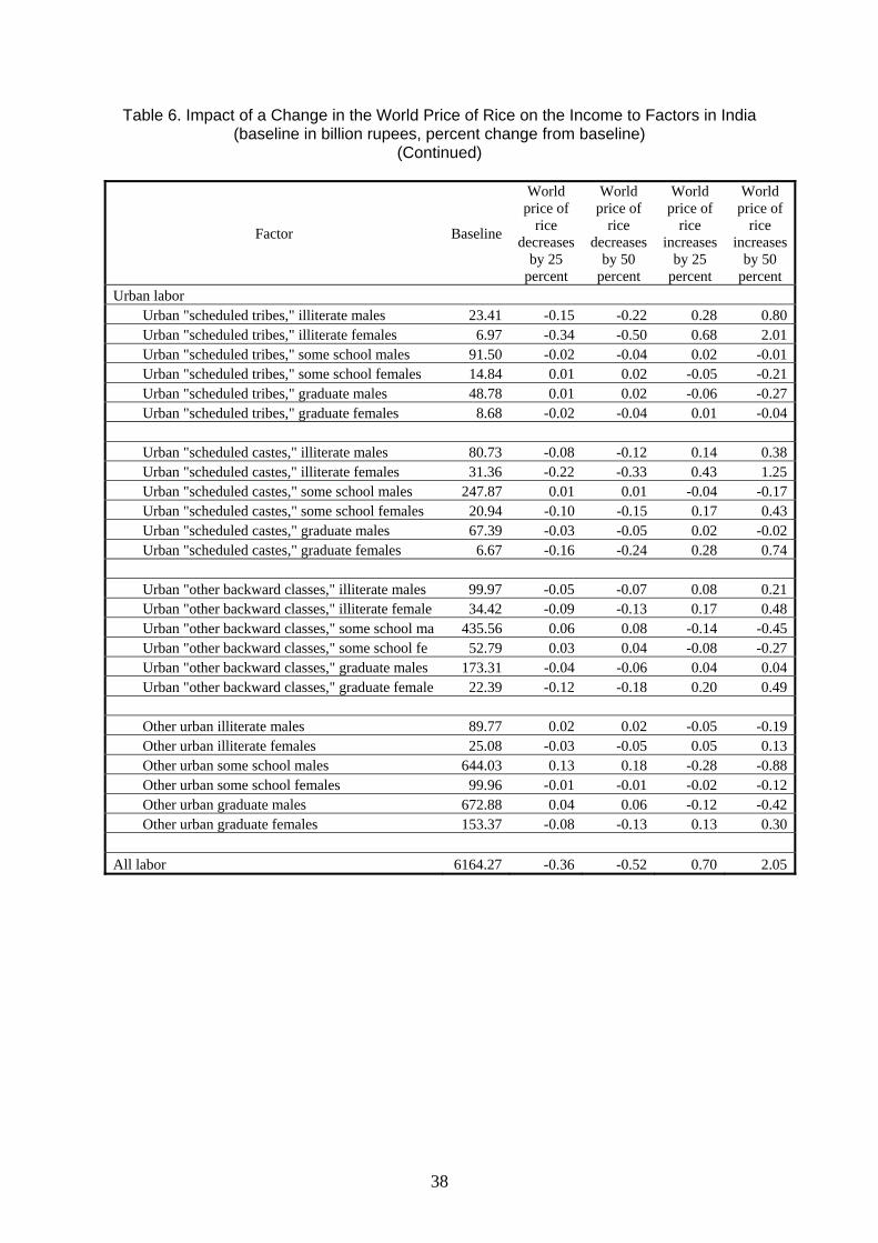
illiterate workers (typically the least skilled) in urban areas decline, as is seen in Table 6.

The distributional impact of an increase in world rice prices on Indian households is

progressive and is larger than that induced by price declines (Table 5, Figure 6). The poorest

rural households see real income gains of 1.4 to 2.2 percent from a 25 percent price increase

and gains of 4 to 6.4 percent from an increase of 50 percent, with the disadvantaged groups

gaining most. All rural households except the richest 10 percent would gain. Similarly, labor

income increases for rural workers at all education levels and for both men and women; the

largest gainers are illiterate workers and disadvantaged groups. The impact of a price increase

on the incomes of urban households is more varied. Some poor households gain while others

7 Other recent work demonstrates how agricultural price shocks can be transmitted through labor and land markets. See, e.g., Dyer, Boucher, and Taylor (2005).

14

lose. The richest households are net losers. Illiterate urban workers from all disadvantaged

groups see their incomes rise, while the results for other urban workers show a mix of small

gains and small losses with no consistent pattern.

Changes in the world price of wheat have much more muted impacts on the Indian

economy than variations in the price of rice. Most macroeconomic variables are almost

unchanged, except for imports, which increase by 1 percent in the case of a 50 percent price

decline (Table 7). Effects at the household level are also smaller than for rice. The negative

impact of a decrease in world wheat prices on rural households is much smaller than that of a

decline in the price of rice, although the pattern is somewhat similar: poor households lose

while richer households gain (Table 8, Figure 7). Urban households experience small gains at

all income levels. Nonetheless, the overall effect could be to increase poverty, as 92 million

rural households in the bottom six deciles of income experience some real income loss, while

only 32 million urban households in the same deciles experience income gains (Tables 8, 1).

Increases in the world price of wheat produce small gains for the poorest groups in

rural areas and small losses for other rural and all urban households (Table 8, Figure 8).

The increase in agricultural prices as simulated here comes through changes in world

market prices, which would have stronger effects on India after it lowers its tariffs. However

another study of the proposals for “special products” and a “special safeguard mechanism” in

the Doha Round treats price increases as a surrogate for government action to mitigate global

price declines through tariff measures (Ivanic and Martin 2006). In our view, an increase in

world prices is not equivalent to a policy-induced domestic price change. However if the

surrogate approach is taken, the impact of Indian government action to shield its domestic

producers from a decline in the world price of rice would unambiguously be to reduce

poverty and improve income distribution. In the case of wheat, government action could also

15

have a net poverty reducing effect, although the determination would require a careful

analysis of the extent of gains and losses in poor and near-poor households.

5. Results of Other Studies of Trade Liberalization and Poverty

Topalova (2005) conducts an ex post study of India’s trade liberalization in the 1990s

using a difference-in-difference approach to poverty reduction across Indian districts. She

finds that regions which were more exposed to trade had less poverty reduction and that the

results were driven by reductions in agricultural rather than manufacturing trade protection.

Hertel et al (2008) conduct ex ante simulations of trade liberalization across fifteen

developing countries (not including India) and find mixed results for poverty. Full global

trade liberalization would reduce poverty in a majority (nine) of the countries studied, while a

more modest Doha round scenario would see poverty increase in a majority (eight) of

countries. Decomposing the drivers of poverty changes under Doha, the authors find that rich

country agricultural reforms increase or leave poverty unchanged in ten countries, while poor

country agricultural reforms do so in five countries. The strongest poverty alleviating effects

(greater than one percent reduction in the poverty headcount at $1/day) come from increased

earnings for agricultural labor in the leading agricultural exporting countries in the study

(Brazil, Chile, Thailand) as a result of rich countries’ reform of their agricultural policies.

These gains are offset to some degree by increases in cost-of-living in those countries as a

result of the same reforms, as more food is exported rather than sold at in the domestic

market. Agricultural trade reforms by poor countries have more muted effects, with the

largest poverty reduction (for Thailand) amounting to about one-third of one percent.

Parikh et al (1995, 1997) and Panda and Quizon (1999) use country-level models of

India to probe the effects of trade liberalization on income distribution and poverty. These

studies found that, in the short run, trade liberalization adversely affects both growth and

16

equity. In the long run, the liberalization of agriculture and manufacturing both have positive

effects on growth, but their distributional effects differ. Liberalization in the manufacturing

sector increases the real incomes of all groups, rich as well as poor, in both rural and urban

sectors. However liberalization in the agricultural sector benefits only upper-income groups

in rural areas and adversely affects all classes in urban areas. The simulation experiments

show that the poor would need to be protected by safety net mechanisms, such as an

expansion of public employment programs. Trade liberalization coupled with safety nets

could lead to a Pareto-improving situation where both rich and poor in both rural and urban

areas gain. In the long run, liberalization helps to modestly accelerate GDP growth (by about

0.6 percent) through a more efficient allocation of resources across sectors and through an

increase in the real investment rate. This occurs because the same nominal savings or

investment rate leads to a higher real investment rate after the relative price of investment

goods falls with the removal of protection on capital goods. The extent of poverty is reduced

in the long run.

Anderson, Martin, and van der Mensbrugghe (2006) carry out an analysis of the

impact of full global free trade in merchandise projected to 2015, using the World Bank’s

recursive dynamic model, known as LINKAGE. Their results show very muted gains for

India (which is the largest country in their “South Asia” aggregation), with real income only

0.4 percent higher in 2015 compared with the baseline case without reform. Agricultural and

food products imports rise by 165 percent, while exports rise by just 53 percent, resulting in

an output loss of about 3.7 percent. Nevertheless, the authors find that the country’s food self-

sufficiency levels remain more or less intact and that there are welfare gains for unskilled

labor and farmers. These results depend strongly on the assumptions chosen by the authors.

In a sensitivity analysis, van der Mensbrugghe, one of the study’s authors, finds losses for

India (that is, “South Asia”) in comparative static results that do not include the dynamic

17

model’s assumption that trade will induce additional investment and productivity gains (van

der Mensbrugghe 2006a, 2006b). India also loses if standard GTAP assumptions about the

elasticity of trade are used, rather than the more responsive elasticities chosen by Anderson,

Martin, and van der Mensbrugghe.

Given the relatively high levels of protection in the Indian economy, it might be

expected that greater opening to trade would lead to much faster growth for the economy

overall, which could contribute to poverty alleviation. However the result of these and other

studies, (e.g., Ganesh-Kumar, Panda, and Burfisher 2006, Polaski 2006) show that the gains

for the Indian economy from multilateral trade liberalization are surprisingly modest. The

distributional and poverty consequences of trade policy changes that expose the economy to

greater price volatility in world agricultural markets thus loom larger against this backdrop.

6. Conclusions

This paper has examined the impact of changes in world agricultural prices on

poverty and income distribution in India. We find that a price decrease for rice, a key crop,

lowers incomes of the poor, with sharp impacts on the poorest households. The negative

effects also carry over to the poorest urban households through the labor market channel.

The impacts are of a magnitude that they could potentially offset most of the gains from Doha

Round found in other studies. Given the very low incomes of most Indian households and

the country’s high poverty rate, this suggests that the question of agricultural trade

liberalization should be evaluated carefully by the Indian government, as even short-term

welfare losses for these households would be highly damaging.

More broadly, our results demonstrate that the impact of world agricultural price

changes on incomes and poverty depends on the specific patterns of production and

consumption in a country and the specific distribution of poverty. We demonstrate that factor

18

markets, particularly labor markets, must be examined in order to understand the full impact

of food price changes on poverty in both rural and urban areas. This focus has been absent in

most studies and in popular discourse on the topic.

It is probable that the poverty impact of agricultural price changes will vary among

developing countries depending on the distribution of poverty, patterns of agricultural

production and consumption, and unskilled labor market characteristics. Therefore

generalizations about the impact of agricultural price changes on poverty are likely to be

misleading. However, given the concentration of poverty in rural areas and in agriculture in

most developing countries, there should be at least an initial presumption that agricultural

price decreases could increase poverty. The presumption currently popular among many

commentators and some economists that policy interventions in agricultural prices—such as

tariffs and price supports—are likely to be poverty increasing finds little support in careful

research and cannot be generalized to all developing countries.

The assumption that the urban poor will always benefit from lower food prices is

found in this study to be invalid for the poorest urban households in India. Other careful

studies of the distributional impact of agricultural price declines induced by trade policy

changes find that the overall impact on poverty can be negative even when the urban poor

gain, because of the greater concentration of poverty in the countryside or other reasons (e.g.,

Ravallion and Lokshin 2004; Hertel and Keeney 2006; Hertel et al. 2006).

There are practical implications for the Doha round negotiations. At least for India,

our findings that decreases in the price of rice, and to a lesser extent, wheat, could increase

and deepen poverty suggest that the government’s concern over potential negative effects of a

Doha agreement on poverty and rural development is well founded. The ability to use a

“special products” designation and invoke a “special safeguard mechanism” would be

necessary instruments for the Indian government to avoid negative effects on the poor in the

19

face of global price declines. Given the varied impact of agricultural price changes on the

poor in developing countries with differing patterns of poverty, production and consumption,

policy discretion should be left to individual countries to deal with the specific impacts of

world agricultural price changes on poverty, rather than having rigid disciplines imposed in

advance.

7. References

Anderson, Kym, William J. Martin, and Dominique van der Mensbrugghe. 2006. “Market and Welfare Implications of Doha Reform Scenarios.” In Agricultural Trade Reform and the Doha Development Agenda, ed. Kym Anderson and William J. Martin. Washington, D.C.: World Bank.

Armington, Paul S. 1969. “A Theory of Demand for Products Distinguished by Place of

Production.” IMF Staff Papers 16: 159–178. Asian Development Bank. 2007. Purchasing Power Parity Preliminary Report. Manila: Asian

Development Bank. Brooks, Jonathan. 2003. “Agricultural Policy Design in Developing Countries: Making Use

of Disaggregated Analysis – Overview Paper.” Paper prepared for the OECD Global Forum on Agriculture, Paris, December 10-11, 2003.

Conforti, Piero. 2004. Price Transmission in Selected Agricultural Markets. Commodity and

Trade Policy Research Working Paper No. 7. Rome: Food and Agriculture Organization of the United Nations.

de Melo, Jaime, and Sherman Robinson. 1989. “Product Differentiation and the Treatment of

Foreign Trade in Computable General Equilibrium Models of Small Economies.” Journal of International Economics 27: 47–67.

Dervis, Kemal, Jaime de Melo, and Sherman Robinson. 1982. General Equilibrium Models

for Development Policy. Cambridge: Cambridge University Press. Devaragan, Shantayanan, Jeffrey D. Lewis, and Sherman Robinson. 1990. “Policy Lessons

from Trade-Focused, Two-Sector Models.” Journal of Policy Modeling 12: 625–657. Dyer, George A., Steve Boucher, and J. Edward Taylor. 2005. “Subsistence Response to

Market Shocks.” Working Paper 05-004, Department of Agricultural and Resource Economics, University of California, Davis.

Ganesh-Kumar, Anand, Manoj Panda, and Mary E. Burfisher. 2006. Reforms in Indian Agro-

Processing and Agriculture Sectors in the Context of Unilateral and Multilateral Trade

20

Agreements. Working Paper WP-2006-011. Mumbai: Indira Gandhi Institute of Development Research.

Hertel, Thomas W. and Jeffrey R. Reimer. 2004. Predicting the Poverty Impacts of Trade

Reform. Policy Research Working Paper 3444. Washington, D.C.: World Bank. Hertel, Thomas. W. and Roman Keeney. 2006. “What Is at Stake: The Relative Importance

of Import Barriers, Export Subsidies and Domestic Support.” In Agricultural Trade Reform and the Doha Development Agenda, ed. Kym Anderson and Will Martin. New York: Palgrave Macmillan.

Hertel, Thomas W., Roman Keeney, Maros Ivanic, and L. Alan Winters. 2008. “Why Isn’t

the Doha Development Agenda More Poverty Friendly?” GTAP Working Paper No. 37. W. Lafayette, Indiana: Center for Global Trade Analysis.

ILO (International Labor Office). 2007. Laborsta Database. http://laborsta.ilo.org/. International Monetary Fund. 2007a. “The Globalization of Labor.” In World Economic

Outlook: Spillovers and Cycles in the Global Economy. Washington, D.C.: International Monetary Fund.

———. 2007b. World Economic Outlook Database.

http://www.imf.org/external/pubs/ft/weo/2007/01/data/index.aspx. Ivanic, Maros, and Will Martin. 2006. “Implications of Agricultural Special Products for

Poverty in Low-Income Countries.” Mimeo. Kilkenny, Maureen. 1991. “Computable General Equilibrium Modeling of Agricultural

Policies: Documentation of the 30-Sector FPGE GAMS Model of the United States.” USDA Economic Research Service Staff Report AGES 9125.

McDonald, Scott. 2005. “Deriving Reduced Form Social Accounting Matrices from a GTAP

based Global Social Accounting Matrix.” Mimeo. McDonald, Scott. 2006. “STAGE: A Static Applied General Equilibrium Model: Technical

Documentation.” Mimeo. (Version 1.1: November 2006.) NCEUS (National Commission for Enterprises in the Unorganised Sector), Ministry of Small

Scale Industries, Government of India. 2007. “Report on Conditions of Work and Promotion of Livelihoods in the Unorganised Sector.” http://nceus.gov.in/

National Sample Survey Organisation, Ministry of Statistics and Programme Implementation,

Government of India. 2000. National Sample Survey (55th Round), July 1999-June 2000.

———. 2005. National Sample Survey (61st Round), July 2004-June 2005. Panda, Manoj. 2007a. “India.” In Beyond Food Production: The Role of Agriculture in

Poverty Reduction, ed. F. Bresciani and A. Valdes. Cheltenham, U.K.: Food and Agriculture Organization of the United Nations and Edward Elgar Publishing.

21

———. 2007b. “Macroeconomic Overview.” In India Development Report 2007, ed. R.

Radhakrishna. New Delhi: Oxford University Press. Panda, Manoj, and Jaime Quizon. 1999. “Growth and Distribution under Trade Liberalization

in India.” Indira Gandhi Institute of Development Research, Mumbai. Forthcoming in a volume edited by A. Guha, A. Lahiri, and K. L. Krishna to be published by NIPFP/Ford Foundation, New Delhi.

Parikh, Kirit S., N. S. S. Narayana, Manoj Panda, and Anand Ganesh-Kumar. 1995.

“Strategies for Agricultural Liberalization: Consequences for Growth, Welfare and Distribution.” Report Submitted to the World Bank, PP-16, Indira Gandhi Institute of Development Research, Mumbai.

———. 1997. “Agricultural Trade Liberalization: Growth, Welfare and Large Country

Effects.” Agricultural Economics 17: 1–20. Planning Commission, Government of India. 2004. “India Vision 2020.” Polaski, Sandra. 2006. Winners and Losers: Impact of the Doha Round on Developing

Countries. Washington, D.C.: Carnegie Endowment for International Peace. Pradhan, Basanta K., and P. K. Roy. 2003. The Well Being of Indian Households: MIMAP

India Survey Report. New Delhi: National Council of Applied Economic Research. Pradhan, Basanta K., M. R. Saluja, and Shalabh K. Singh. 2005. Social Accounting Matrix

for India: Concepts, Construction and Applications. New Delhi: Sage Publications. Pyatt, Graham. 1987. “A SAM Approach to Modelling.” Journal of Policy Modeling 10:

327–352. ———. 1989. “The Method of Apportionment and Accounting Multipliers.” Journal of

Policy Modeling 11: 111–130. Ravallion, Martin, and Michael Lokshin. 2004. Gainers and Losers from Trade Reform in

Morocco. Policy Research Working Paper 3368. Washington, D.C.: World Bank. Reserve Bank of India. 2007. Annual Report 2006–2007.

http://rbidocs.rbi.org.in/rdocs/AnnualReport/PDFs/79542.pdf. Robinson, Sherman, Maureen Kilkenny, and Kenneth Hanson. 1990. “USDA/ERS

Computable General Equilibrium Model of the United States.” USDA Economic Research Service Staff Report AGES 9049.

Taylor, Edward J., Antonio Yúnez-Naude and George Dyer. 2003. “Disaggregated Impacts of

Policy Reform: Description of a Case Study Using Data from the Mexico National Rural Household Survey.” Paper prepared for the OECD Global Forum on Agriculture, Paris, December 10-11, 2003.

22

Topalova, Petia. 2005. “Trade Liberalization, Poverty and Inequality: Evidence from Indian Districts.” NBER Working Paper 11614, Cambridge, Massachusetts: National Bureau of Economic Research.

UNICEF. 2006. “Progress for Children: A Report Card on Nutrition.” No. 4, May.

http://www.unicef.org/progressforchildren/2006n4/files/PFC4_EN_8X11.pdf. United Nations. 2007. UN COMTRADE Database. Accessed using the World Integrated

Trade Solution (WITS), http://wits.worldbank.org. van der Mensbrugghe, Dominique. 2006a. “Estimating the Benefits of Trade Reform: Why

the Numbers Change.” In Trade, Doha, and Development: Window into the Issues, ed. Richard Newfarmer. Washington, D.C.: World Bank.

———. 2006b. “Global Merchandise Trade Reform: Comparing Results with the Linkage

Model.” Paper prepared for the Ninth Annual Conference on Global Economic Analysis of the Global Trade Analysis Project (GTAP), https://www.gtap.agecon.purdue.edu/network/member_display.asp?UserID=415.

World Bank. 2007a. “Commodity Markets Briefs: Rice.”

http://siteresources.worldbank.org/INTGLBPROSPECTSAPRIL/64218944-1111598207001/21359826/rice_EN.pdf.

———. 2007b. “Commodity Markets Briefs: Wheat.”

http://siteresources.worldbank.org/INTGLBPROSPECTSAPRIL/64218944-1111598207001/20911194/wheat_EN.pdf.

———. 2007c. Global Monitoring Report 2007. Washington, D.C.: World Bank. ———. 2007d. World Development Indicators 2007 CD-ROM. Washington, D.C.: World

Bank. World Trade Organization. 2007a. “Countries, alliances, and proposals.” In Agriculture

Negotiations: Backgrounder. http://www.wto.org/english/tratop_e/agric_e/negs_bkgrnd04_groups_e.htm.

———. 2007b. “Risks Lie Ahead Following Stronger Trade in 2006, WTO Reports.” Press

Release, April 12. http://www.wto.org/english/news_e/pres07_e/pr472_e.htm. ———. 2007c. Trade Policy Review: India. WT/TPR/S/182.

http://www.wto.org/english/tratop_e/tpr_e/tp283_e.htm.

23

Appendix A. Description of the India Country Model

The STAGE (Static Applied General Equilibrium) model (CGE) model8 is a member

of the class of single country computable general equilibrium (CGE) models that are

descendants of the approach to CGE modeling described by Dervis et al., (1982) and models

reported by Robinson et al., (1990) and Kilkenny (1991). The model is implemented using

the GAMS (General Algebraic Modeling System) software. The model is a SAM based CGE

model, and the modeling approach has been influenced by Pyatt’s “SAM Approach to

Modeling” (Pyatt, 1988).

The description of the model proceeds in two stages. The first stage is the

identification of the behavioural relationships; while the second stage illustrates the price and

quantity systems embodied within the model.

Behavioral Relationships

The behavioral relationships in this model are a mix of non-linear and linear

relationships that govern how the model’s agents will respond to exogenously determined

changes in the model’s parameters and/or variables.

Households choose the bundles of commodities they consume to maximise utility

where the utility function is a Stone-Geary function that allows for subsistence consumption

expenditures, which is an arguably realistic assumption when there are substantial numbers

of very poor consumers. The households choose their consumption bundles from a set of

‘composite’ commodities that are Constant Elasticity of Substitution (CES) aggregates of

domestically produced and imported commodities, which are imperfect substitutes. This is

the so-called Armington “insight” (Armington, 1969), which allows for product

differentiation via the assumption of imperfect substitution (see Devarajan et al., 1994). The 8 The STAGE model is fully documented in McDonald 2006, available from the author: smcdonald@brookes.ac.uk

24

assumption has the advantage of rendering the model practical by avoiding the extreme

specialisation and price fluctuations associated with other trade assumptions. In this model

the country is assumed to be a price taker for all imported commodities.

Domestic production uses a two-stage production process. In the first stage aggregate

intermediate and aggregate primary inputs are combined using CES technology. At the

second stage intermediate inputs are used in fixed proportions relative to the aggregate

intermediate input used by each activity, while primary inputs are combined to form

aggregate value added using CES technologies, with the optimal ratios of primary inputs

being determined by relative factor prices. The activities are defined as multi-product

activities with commodities differentiated by source activity. Total commodity demands are

determined by the domestic demand for domestically produced commodities and export

demand. Assuming imperfect transformation between the domestic and export commodities

the optimal distribution between the domestic and export markets is determined using

Constant Elasticity of Transformation (CET) functions. The model can be specified as a

small country, i.e., price taker, on all export markets, or selected export commodities can face

downward sloping export demand functions, i.e., a large country assumption.

The model is set up with a range of flexible closure rules. The base model contains

the assumption that all factors are fully employed and mobile; however this assumption is

questionable with respect to unskilled labor in India. We vary the standard assumption with

an alternative labor market closure for unskilled labor in which the real wage is held constant

and the supply of unskilled labor is assumed to be infinitely elastic at that wage. As a result,

it is labor supply that clears the market, and any shock that would otherwise increase

(decrease) the equilibrium wage will instead lead to increased (decreased) employment. The

results we report are for this alternative.

25

Price and Quantity Relationships

Figures A.1 and A.2 provide an overview of the interrelationships between the prices

and quantities. The supply prices of the composite commodities (PQSc) are defined as the

weighted averages of the domestically produced commodities that are consumed domestically

(PDc) and the domestic prices of imported commodities (PMc), which are defined as the

products of the world prices of commodities (PWMc) and the exchange rate (ER) uplifted by

ad valorem import duties (tmc). Consumer prices for commodities (PQDc) are defined as

supply prices plus (ad valorem) sales taxes (tsc). The producer prices of commodities (PXCc)

are weighted averages of the prices received for domestically produced commodities sold on

domestic and export (PEc) markets. The prices received on the export market are the products

of the world price of exports (PWEc) and the exchange rate (ER) less any ad valorem export

duties (tec).

The average price per unit of output received by an activity (PXa) is defined as the

weighted average of the domestic producer prices. The prices of value added (PVAa), i.e., the

amount available to pay primary inputs, are defined as activity prices less indirect taxes (txa)

and payments for intermediate inputs (PINTa), where the (aggregate) intermediate input

prices are defined as the weighted sums of the prices of the inputs (PQDc).

Total demands for the composite commodities, QQc, consist of demands for

intermediate inputs, QINTDc, consumption by households, QCDc, enterprises, QENTDc, and

government, QGDc, gross fixed capital formation, QINVDc, and stock changes, dstocconstc.

Supplies from domestic producers, QDc, plus imports, QMc, meet these demands.

Commodities are delivered to both the domestic and export, QEc, markets subject to

equilibrium conditions that exhaust all domestic commodity production, QXCc. Domestic

production by commodity is an aggregate of the quantities of that commodity produced by a

number of different activities (QXACa,c).

26

Production relationships by activities are defined as nested CES production functions.

The nesting structure is illustrated in lower part of Figure A.2, where, for illustration

purposes only, two intermediate inputs and three primary inputs (FDk,a, FD11,a and FDl2,a) are

identified. Activity output is a CES aggregate of the quantities of aggregate intermediate

inputs (QINTa) and value added (QVAa), while aggregate intermediate inputs are a Leontief

aggregate of the (individual) intermediate inputs and aggregate value added is a CES

aggregate of the quantities of primary inputs demanded by each activity (FDf,a).

27

Appendix B. Description of the Social Accounting Matrix (SAM) and Data for the Model

The Social Accounting Matrix (SAM) reports all the flows of receipts accruing to and

expenditures incurred by all the agents in the economy for a particular year. The agents in the

economy are typically the production sectors, social groups (households), firms, government and

the foreign sector. These flows take place on account of commodity transactions (buying-selling)

between the agents for purposes of consumption, intermediate use, investment, etc., and by way

of inter-agent transfers. The SAM is constructed in two stages. The first is a ‘macro SAM’ that

presents the aggregates of these flows for the economy as a whole. Next is the ‘micro SAM’ that

disaggregates the commodities, activities, factors and households into their respective

components. This top down approach is adopted in preference to the UN System of National

Accounts preferred bottom-up method to ensure that the final micro SAM is consistent with the

published national accounts aggregates.

The Macro SAM

Table B.1 gives the structure of the macro SAM, and the flow values for the year 1998-

99. Most of the data for the macro SAM come from the Input-Output (IO) Table for 1998-99

and from the National Accounts Statistics (NAS), both prepared by the Central Statistical

Organization (CSO), Government of India. It must be noted here that the IO Table is

balanced and is consistent with the NAS data available at the time of its preparation.

However, all the revisions that the NAS undergoes after the preparation of the IO Table are

not carried over to the IO Table. Thus, there are some small differences in the macro

aggregates between these two sources. Where such differences are observed, we defer to the

values in the IO Table due to its internal consistency across its rows and columns. These two

data sources are supplemented with data on government transfers from Pradhan et al (2005).

28

Some of the entries of the macro SAM are derived residually to maintain row – column

balance. In the rest of world (RoW) account, data are available for all the row entries, and for

all the column entries except capital transfers to RoW. The latter was then obtained residually

as the difference between the row total and sum of column entries for which we have data.

Next, we worked out the net household savings in the gross fixed capital account row

residually as the difference between the column total (for which we had all the information)

and the sum of the row entries for which we had data. Factor payments to households, firms

and government were also derived sequentially following a similar procedure.

The Micro SAM

The macro SAM gives a snap shot of the economy and also provides several control totals

for the micro SAM. The micro SAM distinguishes 115 commodities, 115 activities, 49

factors and 352 households. The 115 commodities and 115 activities directly correspond to

the IO Table. With regard to factors, we distinguish 1 capital (non-labor) and 48 labor types

based on the following characteristics:

• location (rural / urban)

• social group (“scheduled tribes” / “scheduled castes” / “other backward classes”/

others)

• education level (illiterate / education up to high school / graduates and above)

• sex (male / female).

Households are distinguished into 352 types based on the following characteristics:

• location (rural / urban)

• social group (“scheduled tribes” / “scheduled castes” / “other backward classes” /

others)

29

• region (north / east / west / south)

• eleven mean per capita expenditure (MPCE) classes (the first nine deciles in the

sample, and the top decile further split into 91-95 percentile and 96 to 100 percentile).

Database

The data for the micro SAM are from (a) the IO Table mentioned earlier, (b) unit

(household) level data from sample surveys on Consumer Expenditure and Employment /

Unemployment 55th Round for 1999-2000 carried out by the National Sample Survey

Organization (NSSO), (c) Pradhan and Roy (2003), and (d) Pradhan et al (2005). The IO

Table gives data on intermediate flows (use matrix), sectoral value added, the commodity

composition (make) matrix, and commodity-wise total private consumption and other final

demand vectors. Of these, the use matrix, make matrix, and the final demands (except

private) are used directly in the micro SAM.

Distribution of Factor Income

The sectoral value added from the IO Table is distributed first into labor and capital

(non-labor) based on the labor-capital shares derived from Pradhan et al (2005). The value

added accruing to labor is then distributed to the 48 labor types based on information from

the NSSO Employment / Unemployment survey. The survey provides information on

household characteristics (location, social group, region and mean per capita expenditure),

characteristics of each household member (age, sex and education level), employment status

(usually employed / unemployed) and for those who are employed, the sector of usual

employment (at NIC 5-digit level) and the total wages received during the week preceding

the survey. From the unit level data, we first generate the labor types as described earlier.

Second, for each labor type the sector of employment was mapped from the NIC 5-digit level

to our 115 sector level, and the deployment of each labor type by sector was generated. Third,

30

for each labor type an average daily wage rate was constructed from the data on wages

available at the unit level. With the sectoral employment and average wage information we

could obtain sectoral wage income for each labor type. The structure implied by this data was

used to disaggregate the total sectoral labor value added from the IO Table across our 48

labor types by adjusting the wage rate for each labor type.

Household Labor Endowment

The household characteristics reported in the Employment / Unemployment survey

enables us to construct household groups as defined above. For each of these household

categories, we then develop the total endowment of different types of labor from the unit

level information. Given the characteristics used to classify labor types, every household

category will have more than one labor type. This information on labor endowments and the

wage rates obtained above are used to generate total labor income for each household

category.

Household Consumption Expenditure

The NSSO Consumption Expenditure provides information on household

characteristics (location, social group, region and mean per capita expenditure) and also

detailed information on commodity-wise consumptions at the household level. The common

information on household characteristics from the two NSSO surveys enables us to use a

consistent definition of household categories across both surveys. Thus, for our 352

household categories we develop the commodity-wise consumption expenditures by mapping

the detailed commodity list in the survey to the 115 commodities in the IO Table. It is well

known that the aggregate total consumption expenditure from survey usually do not tally with

the estimates of consumption from the NAS data due to differences in the methodology of the

two approaches and their coverage. Since the IO Table is the main basis for the SAM, we use

31

the consumption structure across households from the survey and apply them on the

commodity-wise total private consumption expenditure reported in the IO Table. This enables

us to maintain internal consistency in the SAM.

Household Income Expenditure Balance

Thus far we have only labor income and consumption expenditure for each

household, which is insufficient to close the income-expenditure accounts for households.

Detailed data on savings, transfers, and non-labor income are not available for our household

categories. The NCAER-MIMAP Survey (Pradhan and Roy 2003) allows us to compute

decile-wise savings / dis-savings rates for rural and urban areas separately. We have assumed

that these rates prevail for each decile within rural and urban independent of other household

characteristics namely region and social group. Thus we could generate household savings.

Total household income was then obtained with certain assumptions on the distribution of

direct taxes and transfers. Given this total income and the wage income estimated earlier,

income from capital (non-labor factors) was obtained for all the household categories.

32

Table 1. Distribution of Households in the Indian Population, Total

Household Group Number Share Rural

Rural "scheduled tribes," income 0-30 percent 8,070,164 4.28Rural "scheduled tribes," income 31-60 percent 4,119,474 2.19Rural "scheduled tribes," income 61-90 percent 2,378,644 1.26Rural "scheduled tribes," income >90 percent 372,694 0.20 Rural "scheduled castes," income 0-30 percent 13,393,888 7.11Rural "scheduled castes," income 31-60 percent 9,300,193 4.94Rural "scheduled castes," income 61-90 percent 5,545,583 2.94Rural "scheduled castes," income >90 percent 923,481 0.49 Rural "other backward classes," income 0-30 percent 17,932,008 9.52Rural "other backward classes," income 31-60 percent 16,982,923 9.01Rural "other backward classes," income 61-90 percent 13,312,988 7.07Rural "other backward classes," income >90 percent 2,697,944 1.43 Other rural, income 0-30 percent 9,042,016 4.80Other rural, income 31-60 percent 13,205,395 7.01Other rural, income 61-90 percent 14,608,818 7.75Other rural, income >90 percent 5,278,772 2.80

Urban

Urban "scheduled tribes," income 0-30 percent 860,491 0.46Urban "scheduled tribes," income 31-60 percent 515,517 0.27Urban "scheduled tribes," income 61-90 percent 341,136 0.18Urban "scheduled tribes," income >90 percent 77,309 0.04 Urban "scheduled castes," income 0-30 percent 3,736,578 1.98Urban "scheduled castes," income 31-60 percent 2,110,141 1.12Urban "scheduled castes," income 61-90 percent 1,110,004 0.59Urban "scheduled castes," income >90 percent 160,863 0.09 Urban "other backward classes," income 0-30 percent 6,256,092 3.32Urban "other backward classes," income 31-60 percent 4,850,576 2.57Urban "other backward classes," income 61-90 percent 3,604,215 1.91Urban "other backward classes," income >90 percent 730,890 0.39 Other urban, income 0-30 percent 6,114,311 3.24Other urban, income 31-60 percent 7,802,559 4.14Other urban, income 61-90 percent 9,314,989 4.94Other urban, income >90 percent 3,680,458 1.95

All households 188,431,114 100.00

33

Table 2. Distribution of Rural Households

Household Group Number Share

Rural "scheduled tribes," income 0-30 percent 8,070,164 5.88Rural "scheduled tribes," income 31-60 percent 4,119,474 3.00Rural "scheduled tribes," income 61-90 percent 2,378,644 1.73Rural "scheduled tribes," income >90 percent 372,694 0.27 Rural "scheduled castes," income 0-30 percent 13,393,888 9.76Rural "scheduled castes," income 31-60 percent 9,300,193 6.78Rural "scheduled castes," income 61-90 percent 5,545,583 4.04Rural "scheduled castes," income >90 percent 923,481 0.67 Rural "other backward classes," income 0-30 percent 17,932,008 13.07Rural "other backward classes," income 31-60 percent 16,982,923 12.38Rural "other backward classes," income 61-90 percent 13,312,988 9.71Rural "other backward classes," income >90 percent 2,697,944 1.97 Other rural, income 0-30 percent 9,042,016 6.59Other rural, income 31-60 percent 13,205,395 9.63Other rural, income 61-90 percent 14,608,818 10.65Other rural, income >90 percent 5,278,772 3.85

All rural households 137,164,985 100.00

34

Table 3. Distribution of Urban Households

Household Group Number Share

Urban "scheduled tribes," income 0-30 percent 860,491 1.68Urban "scheduled tribes," income 31-60 percent 515,517 1.01Urban "scheduled tribes," income 61-90 percent 341,136 0.67Urban "scheduled tribes," income >90 percent 77,309 0.15 Urban "scheduled castes," income 0-30 percent 3,736,578 7.29Urban "scheduled castes," income 31-60 percent 2,110,141 4.12Urban "scheduled castes," income 61-90 percent 1,110,004 2.17Urban "scheduled castes," income >90 percent 160,863 0.31 Urban "other backward classes," income 0-30 percent 6,256,092 12.20Urban "other backward classes," income 31-60 percent 4,850,576 9.46Urban "other backward classes," income 61-90 percent 3,604,215 7.03Urban "other backward classes," income >90 percent 730,890 1.43 Other urban, income 0-30 percent 6,114,311 11.93Other urban, income 31-60 percent 7,802,559 15.22Other urban, income 61-90 percent 9,314,989 18.17Other urban, income >90 percent 3,680,458 7.18

All urban households 51,266,129 100.00

Note: Data for Tables 1, 2, and 3 are from the "Household Schedule: Consumer Expenditure" in National Sample Survey Organisation, National Sample Survey (55th Round), July 1999-June 2000. The number of households in each category are scaled from the sample to the population level using the multipliers given in the survey.

35

Table 4. Impact of a Change in the World Price of Rice on India's Economy

(percent change from baseline)

Macroeconomic indicator World price of rice decreases by 25 percent

World price of rice decreases by 50 percent

World price of rice increases by 25 percent

World price of rice increases by 50 percent

Private consumption -0.16 -0.24 0.30 0.84 Government consumption -0.09 -0.12 0.17 0.52 Investment consumption -0.19 -0.28 0.39 1.20 Absorption -0.16 -0.24 0.31 0.89 Import demand -0.88 -1.28 1.82 5.62 Export supply -0.64 -1.24 0.60 1.08 Total domestic production -0.12 -0.17 0.23 0.70

36

Table 5. Impact of a Change in the World Price of Rice on the Real Incomes of Indian Households

(percent change in real income relative to baseline nominal income to households)

Household Group

World price of

rice decreases

by 25 percent

World price of

rice decreases

by 50 percent

World price of

rice increases

by 25 percent

World price of

rice increases

by 50 percent

Rural Rural "scheduled tribes," income 0-30 percent -1.13 -1.65 2.20 6.40Rural "scheduled tribes," income 31-60 percent -0.60 -0.89 1.16 3.32Rural "scheduled tribes," income 61-90 percent -0.20 -0.29 0.36 0.98Rural "scheduled tribes," income >90 percent 0.01 0.02 -0.04 -0.17 Rural "scheduled castes," income 0-30 percent -0.95 -1.40 1.85 5.36Rural "scheduled castes," income 31-60 percent -0.76 -1.12 1.49 4.35Rural "scheduled castes," income 61-90 percent -0.31 -0.46 0.59 1.69Rural "scheduled castes," income >90 percent 0.02 0.03 -0.05 -0.19 Rural "other backward classes," income 0-30 percent -0.78 -1.14 1.50 4.33Rural "other backward classes," income 31-60 percent -0.70 -1.03 1.38 4.02Rural "other backward classes," income 61-90 percent -0.46 -0.67 0.90 2.64Rural "other backward classes," income >90 percent 0.00 0.00 -0.01 -0.06 Other rural, income 0-30 percent -0.73 -1.08 1.41 4.05Other rural, income 31-60 percent -0.62 -0.91 1.21 3.49Other rural, income 61-90 percent -0.46 -0.67 0.89 2.60Other rural, income >90 percent -0.07 -0.10 0.12 0.34

Urban

Urban "scheduled tribes," income 0-30 percent -0.12 -0.18 0.20 0.50Urban "scheduled tribes," income 31-60 percent -0.04 -0.06 0.05 0.09Urban "scheduled tribes," income 61-90 percent 0.01 0.01 -0.03 -0.11Urban "scheduled tribes," income >90 percent 0.02 0.03 -0.05 -0.18 Urban "scheduled castes," income 0-30 percent -0.10 -0.15 0.17 0.43Urban "scheduled castes," income 31-60 percent -0.02 -0.03 0.01 -0.02Urban "scheduled castes," income 61-90 percent 0.01 0.01 -0.03 -0.13Urban "scheduled castes," income >90 percent 0.02 0.03 -0.05 -0.17 Urban "other backward classes," income 0-30 percent -0.02 -0.03 0.01 -0.04Urban "other backward classes," income 31-60 percent 0.05 0.07 -0.13 -0.42Urban "other backward classes," income 61-90 percent 0.07 0.10 -0.16 -0.50Urban "other backward classes," income >90 percent 0.04 0.06 -0.10 -0.31 Other urban, income 0-30 percent 0.03 0.05 -0.10 -0.37Other urban, income 31-60 percent 0.09 0.13 -0.20 -0.63Other urban, income 61-90 percent 0.11 0.16 -0.23 -0.72Other urban, income >90 percent 0.09 0.13 -0.19 -0.58

Total -0.13 -0.19 0.23 0.64

37

Table 6. Impact of a Change in the World Price of Rice on the Income to Factors in India (baseline in billion rupees, percent change from baseline)

Factor Baseline

World price of

rice decreases

by 25 percent

World price of

rice decreases

by 50 percent

World price of

rice increases

by 25 percent

World price of

rice increases

by 50 percent

Capital 8483.87 -0.05 -0.08 0.08 0.17 Rural labor

Rural "scheduled tribes," illiterate males 78.97 -1.01 -1.47 2.03 6.06Rural "scheduled tribes," illiterate females 60.00 -1.10 -1.60 2.22 6.62Rural "scheduled tribes," some school males 144.56 -0.91 -1.32 1.82 5.45Rural "scheduled tribes," some school females 32.82 -0.98 -1.43 1.97 5.90Rural "scheduled tribes," graduate males 23.59 -0.33 -0.49 0.64 1.83Rural "scheduled tribes," graduate females 1.75 -1.07 -1.56 2.14 6.37 Rural "scheduled castes," illiterate males 134.00 -0.96 -1.39 1.93 5.76Rural "scheduled castes," illiterate females 73.52 -1.14 -1.66 2.30 6.87Rural "scheduled castes," some school males 255.35 -0.79 -1.15 1.59 4.73Rural "scheduled castes," some school females 37.21 -0.81 -1.18 1.62 4.83Rural "scheduled castes," graduate males 40.03 -0.44 -0.65 0.87 2.53Rural "scheduled castes," graduate females 3.74 -0.32 -0.48 0.61 1.73 Rural "other backward classes," illiterate males 184.27 -0.89 -1.30 1.79 5.35Rural "other backward classes," illiterate female 111.60 -1.00 -1.45 2.01 6.01Rural "other backward classes," some school ma 460.39 -0.69 -1.01 1.39 4.14Rural "other backward classes," some school fe 98.46 -0.72 -1.06 1.45 4.33Rural "other backward classes," graduate males 85.99 -0.47 -0.70 0.93 2.70Rural "other backward classes," graduate female 7.32 -0.39 -0.57 0.75 2.16 Other rural illiterate males 123.14 -0.91 -1.32 1.83 5.46Other rural illiterate females 77.63 -0.86 -1.25 1.72 5.12Other rural some school males 566.43 -0.72 -1.05 1.44 4.28Other rural some school females 168.06 -0.63 -0.93 1.26 3.74Other rural graduate males 222.37 -0.41 -0.60 0.80 2.32Other rural graduate females 20.41 -0.30 -0.44 0.56 1.59

38

Table 6. Impact of a Change in the World Price of Rice on the Income to Factors in India (baseline in billion rupees, percent change from baseline)

(Continued)

Factor Baseline

World price of

rice decreases

by 25 percent

World price of

rice decreases

by 50 percent

World price of

rice increases

by 25 percent

World price of

rice increases

by 50 percent

Urban labor Urban "scheduled tribes," illiterate males 23.41 -0.15 -0.22 0.28 0.80Urban "scheduled tribes," illiterate females 6.97 -0.34 -0.50 0.68 2.01Urban "scheduled tribes," some school males 91.50 -0.02 -0.04 0.02 -0.01Urban "scheduled tribes," some school females 14.84 0.01 0.02 -0.05 -0.21Urban "scheduled tribes," graduate males 48.78 0.01 0.02 -0.06 -0.27Urban "scheduled tribes," graduate females 8.68 -0.02 -0.04 0.01 -0.04 Urban "scheduled castes," illiterate males 80.73 -0.08 -0.12 0.14 0.38Urban "scheduled castes," illiterate females 31.36 -0.22 -0.33 0.43 1.25Urban "scheduled castes," some school males 247.87 0.01 0.01 -0.04 -0.17Urban "scheduled castes," some school females 20.94 -0.10 -0.15 0.17 0.43Urban "scheduled castes," graduate males 67.39 -0.03 -0.05 0.02 -0.02Urban "scheduled castes," graduate females 6.67 -0.16 -0.24 0.28 0.74 Urban "other backward classes," illiterate males 99.97 -0.05 -0.07 0.08 0.21Urban "other backward classes," illiterate female 34.42 -0.09 -0.13 0.17 0.48Urban "other backward classes," some school ma 435.56 0.06 0.08 -0.14 -0.45Urban "other backward classes," some school fe 52.79 0.03 0.04 -0.08 -0.27Urban "other backward classes," graduate males 173.31 -0.04 -0.06 0.04 0.04Urban "other backward classes," graduate female 22.39 -0.12 -0.18 0.20 0.49 Other urban illiterate males 89.77 0.02 0.02 -0.05 -0.19Other urban illiterate females 25.08 -0.03 -0.05 0.05 0.13Other urban some school males 644.03 0.13 0.18 -0.28 -0.88Other urban some school females 99.96 -0.01 -0.01 -0.02 -0.12Other urban graduate males 672.88 0.04 0.06 -0.12 -0.42Other urban graduate females 153.37 -0.08 -0.13 0.13 0.30

All labor 6164.27 -0.36 -0.52 0.70 2.05

39

Table 7. Impact of a Change in the World Price of Wheat on India's Economy (percent change from baseline)

Macroeconomic indicator

World price of wheat

decreases by 25 percent

World price of wheat

decreases by 50 percent

World price of wheat

increases by 25 percent

World price of wheat

increases by 50 percent

Private consumption 0.03 0.10 -0.02 -0.03 Government consumption 0.00 0.01 0.00 0.00 Investment consumption 0.00 0.00 0.00 0.00 Absorption 0.02 0.06 -0.01 -0.02 Import demand 0.27 1.00 -0.12 -0.19 Export supply 0.12 0.33 -0.07 -0.13 Total domestic production 0.00 0.01 0.00 0.00

40

Table 8. Impact of a Change in the World Price of Wheat on Real Incomes of Indian Households

(percent change in real income relative to baseline nominal income to households)

Household Group

World price of wheat

decreases by 25

percent

World price of wheat

decreases by 50

percent

World price of wheat

increases by 25

percent

World price of wheat

increases by 50

percent Rural

Rural "scheduled tribes," income 0-30 percent -0.08 -0.22 0.05 0.09Rural "scheduled tribes," income 31-60 percent -0.01 -0.01 0.00 0.01Rural "scheduled tribes," income 61-90 percent 0.04 0.11 -0.02 -0.04Rural "scheduled tribes," income >90 percent 0.04 0.10 -0.02 -0.04 Rural "scheduled castes," income 0-30 percent -0.04 -0.10 0.02 0.04Rural "scheduled castes," income 31-60 percent -0.04 -0.11 0.03 0.05Rural "scheduled castes," income 61-90 percent 0.01 0.04 -0.01 -0.01Rural "scheduled castes," income >90 percent 0.04 0.11 -0.02 -0.04 Rural "other backward classes," income 0-30 percent -0.02 -0.04 0.01 0.02Rural "other backward classes," income 31-60 percent -0.04 -0.11 0.03 0.05Rural "other backward classes," income 61-90 percent -0.03 -0.09 0.02 0.04Rural "other backward classes," income >90 percent 0.03 0.08 -0.02 -0.03 Other rural, income 0-30 percent -0.01 -0.02 0.01 0.01Other rural, income 31-60 percent -0.02 -0.04 0.01 0.02Other rural, income 61-90 percent -0.02 -0.06 0.02 0.03Other rural, income >90 percent 0.01 0.04 -0.01 -0.01

Urban Urban "scheduled tribes," income 0-30 percent 0.06 0.18 -0.04 -0.06Urban "scheduled tribes," income 31-60 percent 0.05 0.14 -0.03 -0.05Urban "scheduled tribes," income 61-90 percent 0.04 0.11 -0.02 -0.04Urban "scheduled tribes," income >90 percent 0.03 0.09 -0.02 -0.03 Urban "scheduled castes," income 0-30 percent 0.07 0.19 -0.04 -0.07Urban "scheduled castes," income 31-60 percent 0.06 0.16 -0.03 -0.06Urban "scheduled castes," income 61-90 percent 0.04 0.12 -0.03 -0.05Urban "scheduled castes," income >90 percent 0.03 0.09 -0.02 -0.03 Urban "other backward classes," income 0-30 percent 0.07 0.20 -0.04 -0.07Urban "other backward classes," income 31-60 percent 0.06 0.18 -0.04 -0.07Urban "other backward classes," income 61-90 percent 0.05 0.14 -0.03 -0.05Urban "other backward classes," income >90 percent 0.03 0.09 -0.02 -0.04 Other urban, income 0-30 percent 0.07 0.21 -0.05 -0.08Other urban, income 31-60 percent 0.06 0.18 -0.04 -0.07Other urban, income 61-90 percent 0.05 0.15 -0.03 -0.06Other urban, income >90 percent 0.04 0.12 -0.03 -0.05

Total 0.03 0.07 -0.02 -0.03

41

World Bank $1/day

World Bank $1/day *

World Bank $2/day

World Bank $2/day *

National poverty line

* Using revised PPP estimates (forthcoming)

Number of persons (millions) Percentage of population

Figure 1. Poverty in India, 2004-2005

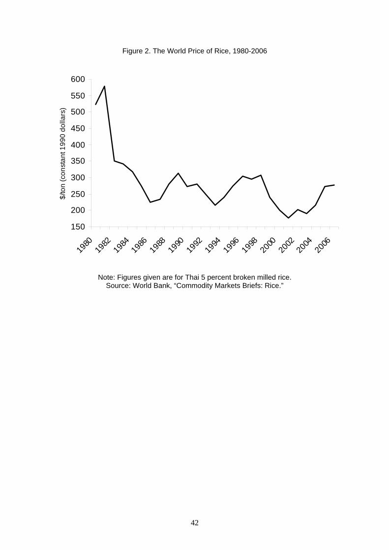
42

Figure 2. The World Price of Rice, 1980-2006

150

200

250

300

350

400

450

500

550

600

1980

1982

1984

1986

1988

1990

1992

1994

1996

1998

2000

2002

2004

2006

$/to

n (c

onst

ant 1

990

dolla

rs)

Note: Figures given are for Thai 5 percent broken milled rice. Source: World Bank, “Commodity Markets Briefs: Rice.”

43

Figure 3. The World Price of Wheat, 1980-2006

100

125

150

175

200

225

1980

1982

1984

1986

1988

1990

1992

1994

1996

1998

2000

2002

2004

2006

$/m

etric

ton

(con

stan

t 199

0 do

llars

)

Note: Figures given are for U.S. hard red winter wheat varieties. Source: World Bank, “Commodity Markets Briefs: Wheat.”

44

UrbanRural

Scheduled Tribes Others

Other Backward Classes

Scheduled Castes

Scheduled Tribes Others

Other Backward Classes

Scheduled Castes

25% decrease

50% decrease

Figure 4. Impact of a Decrease in the World Price of Rice on Indian Households (percent change in real income relative to baseline nominal income to households)

45

-14.00

-12.00

-10.00

-8.00

-6.00

-4.00

-2.00

0.00

2.00

Rice sector Agriculturalsector

Manufacturingsector

Services sector

25% decrease

50% decrease

Figure 5. Impact of a Decrease in the World Price of Rice on the Demand for Indian Labor (percent change in demand for labor relative to baseline)

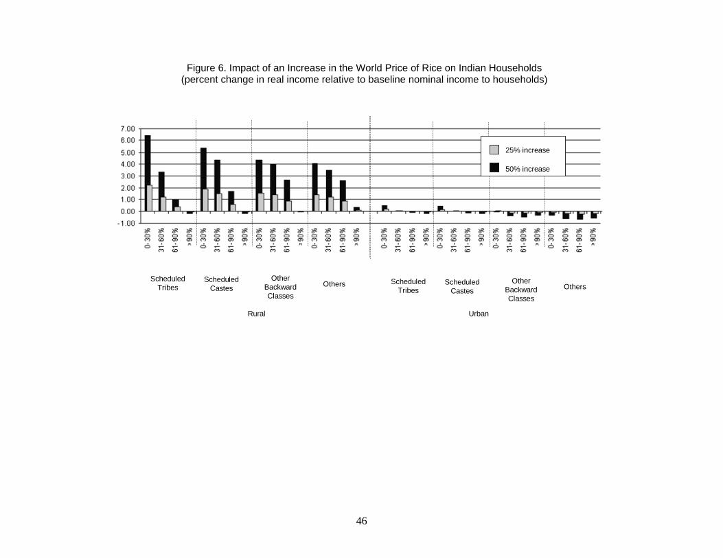
46

UrbanRural

Scheduled Tribes Others

Other Backward Classes

Scheduled Castes

Scheduled Tribes Others

Other Backward Classes

Scheduled Castes

25% increase

50% increase

Figure 6. Impact of an Increase in the World Price of Rice on Indian Households (percent change in real income relative to baseline nominal income to households)

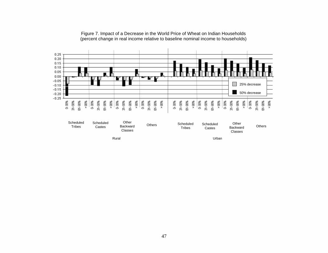
47

UrbanRural

Scheduled Tribes Others

Other Backward Classes

Scheduled Castes

Scheduled Tribes Others

Other Backward Classes

Scheduled Castes

25% decrease

50% decrease

Figure 7. Impact of a Decrease in the World Price of Wheat on Indian Households (percent change in real income relative to baseline nominal income to households)

48

UrbanRural

Scheduled Tribes Others

Other Backward Classes

Scheduled Castes

Scheduled Tribes Others

Other Backward Classes

Scheduled Castes

25% increase

50% increase

Figure 8. Impact of an Increase in the World Price of Wheat on Indian Households (percent change in real income relative to baseline nominal income to households)

49

Table B.1. Macroeconomic Social Accounting Matrix for India, 1998-99 (Rupees crore)

Note: 1 crore = 10 millions.

Commod-ity Activity Factors Households Private

Firms Public Firms

Direct taxes

Import duties

Export subsidies

Domestic net

indirect taxes

Govern-ment

Gross fixed

capital

Changes in stocks

Rest of world Total

Commodity 0 1400115 0 1189267 0 0 0 0 0 0 214032 395147 -2125 199691 3396127 Activity 2998241 0 0 0 0 0 0 0 0 0 0 0 0 0 2998241 Factors 0 1598127 0 0 0 0 0 0 0 0 0 0 0 8133 1606260 Households 0 0 1322790 0 0 0 0 0 0 0 118430 0 0 43242 1484463 Private Firms 0 0 40250 0 0 0 0 0 0 0 5722 0 0 0 45972

Public Firms 0 0 15129 0 0 0 0 0 0 0 0 0 0 0 15129 Direct taxes 0 0 0 28317 24529 0 0 0 0 0 0 0 0 0 52846 Import duties 40668 0 0 0 0 0 0 0 0 0 0 0 0 0 40668

Export subsidies -697 0 0 0 0 0 0 0 0 0 0 0 0 0 -697

Domestic net indirect taxes

111587 0 0 0 0 0 0 0 0 0 0 0 0 0 111587

Government 0 0 36923 0 0 0 52846 40668 -697 111587 0 0 0 0 241327 Gross fixed capital 0 0 168066 266879 21443 15129 0 0 0 0 -99530 0 0 21035 393022

Changes in stocks 0 0 0 0 0 0 0 0 0 0 0 -2125 0 0 -2125

Rest of world 246327 0 23101 0 0 0 0 0 0 0 2673 0 0 0 272101

Total 3396126 2998242 1606260 1484463 45972 15129 52846 40668 -697 111587 241327 393022 -2125 272101

50

Table B.2. Overview of the Indian Economy as Represented in the India Model (Domestic production by industry in rupees and percent share)

Industry Rupees (billion) Share of total economy

Rice 641.60 2.23Wheat 449.54 1.56Plant-based fibers 143.72 0.50Oil seeds 168.08 0.58Other crops 1,645.26 5.72Other animal products 558.36 1.94 Coal 246.22 0.86Oil and gas 131.49 0.46 Dairy products 478.16 1.66Vegetable oils and fats 376.14 1.31Other food products 1,613.64 5.61 Textiles 1,067.74 3.71Wearing apparel 129.81 0.45Petroleum products 498.72 1.73Chemicals 1,856.07 6.45Minerals and metals 1,428.50 4.97Vehicles and other transport equipment 509.17 1.77Other manufacturing 2,711.53 9.43 Utilities 1,205.66 4.19Construction 2,085.46 7.25Trade and transportation 4,938.71 17.17Dwellings 805.57 2.80Public administration 2,151.50 7.48Services 2,919.27 10.15 Total production 28,759.92 100

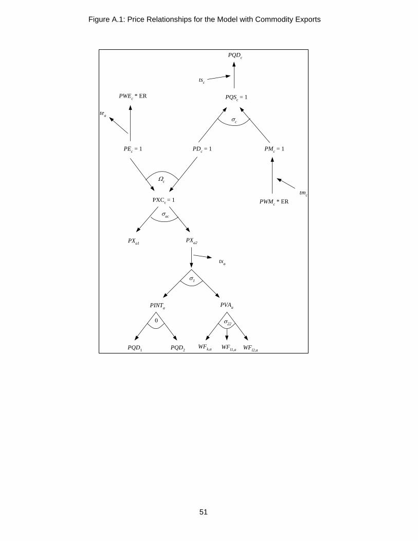
51

Figure A.1: Price Relationships for the Model with Commodity Exports

PDc = 1

PQSc = 1

PMc = 1

PWMc * ERtmc

σc

PXCc = 1

PEc = 1

PWEc * ER

tea

Ωc

tsc

PQDc

PXa1 PXa2

σac

σ22

PQD1

PVAa

WFk,a

0

WFl1,aPQD2

PINTa

σ1

WFl2,a

txa

52

Figure A.2: Quantity Relationships for the Model

QDc

QQc

QXCc

QMc

QINVDc

QGDc

QCDc

QINTDc

QENTDc

QXACa1,c

QEc

Ωc

σc

QXACa2,c

σac

σ22

QINTa QVAa

FDl1,aFDk,a

0

comactactcoc1,a*QINTa

σ1

FDl2,acomactactcoc2,a

*QINTa

QXACa2,c2

QXa2

0