Policy Consequences of Direct Legislation in the … Consequences of Direct Legislation in the States Theory, Empirical Models and Evidence ... Phil Paolino, and

Policy Consequences of Direct Legislation in theStates

Theory, Empirical Models and Evidence�

Simon HugDepartment of Government

University of Texas at Austin�

Paper prepared for presentation at theAnnual meeting of the Public Choice Society

San Antonio, March 8-11, 2001

First version: January 2001, this version: February 19, 2001Rough first draft: please be merciful

Abstract

Most theoretical models predict that institutions allowing for direct legisla-tion should lead, on average, to policies more closely reflecting the wishes ofthe voters. While some agreement exists at the theoretical level about the ex-pected policy consequences of direct legislation, empirical evidence has beenscant so far. In this paper I discuss the reasons for this scantness of empiricalevidence, namely the intricacies of the adequate empirical model to test the theo-retical proposition, and suggest possible solutions to this problem. Re-analyzinga dataset with which some authors have found no evidence in support of the the-oretical claim, I show that with better adapted empirical models we find resultsin synch with our theoretical expectations. Thus, policies in states that allow fordirect legislation reflect on average more closely the voters’ wishes.

�Thanks are due to Chris Achen, Mel Hinich, Tse-Min Lin, John Matsusaka, Phil Paolino, and

George Tsebelis for enlightening discussions on the intricacies of the statistical issues in this paper, andTed Lascher for sharing his dataset. Partial financial support by the Swiss National Science Founda-tion (Grants No. 8210-046545 and 5004-0487882/1) is gratefully acknowledged. I assume responsi-bility for all remaining flaws and errors. Future versions and additional analyses will be available athttp://uts.cc.utexas.edu/simonhug/pcdls/�

Burdine 564; Austin, TX 78712-1087; USA; phone +1 512 232 7273; fax: +1 512 471 1061; email:[email protected].

1

1 Introduction

Direct legislation has no good press, currently. Journalists (e.g., Schrag 1998 and

Broder 2000), as well as some observers (e.g., Smith 1998) find much at fault with

policies adopted in processes of citizen-lawmaking. Implicit in their assessment is the

assumption that policies in states allowing for direct legislation differ from policies

adopted in states not allowing citizens to propose and vote on ballot measures.

Both the descriptive and theoretical literature on direct legislation largely concurs

with this view. Nevertheless, the effect of institutions of direct legislation on policies

has proven more controversial on the empirical level. In this paper I argue that this

controversy is largely due to missspecfications in the empirical models used to assess

the effect of direct legislation. More precisely, most theoretical models suggest that

policies in states allowing for direct legislation should be biased toward the preferred

policy of the median voter.1 This bias obviously depends on what the policy would

have been in the absence of institutions of direct legislation. Hence, when comparing

policies across states with or without direct legislation it is necessary to control for the

voters’ preferences, since these determine the direction of the bias.

But most empirical specifications used in the literature to assess the effect of direct

legislation fail to take this into consideration. Hence, the results obtained are often

biased. While for some empirical specifications it is relatively easy to determine the

bias, in others this proves elusive. Thus, empirical models taking into account the

theoretically derived prediction of the effect of direct legislation should address these

problems directly.

I propose in this paper two empirical models which derive directly from the theo-

retically implied predictions on the effect of direct legislation. Both of them are based

on one restrictive assumption. In the empirical evaluation both yield, however, very

similar results and support the theoretical implication on the effect of direct legislation.

The paper proceeds as follows. In the next section I review very briefly the lit-

erature on the policy effects of direct legislation. In section three I present first the

theoretically implied empirical model, before discussing specifications that have been

employed in the literature. I demonstrate that almost all of these specifications are

based on erroneous assumptions which inevitably result in biases in the estimated co-

1Obviously, the notion of median voter only applies in contexts where the policy outcome reflects aone-dimensional policy space. Hug and Tsebelis (2000) and Tsebelis (2000) propose ways in which thegeneral theoretical ideas discussed in this paper apply in multidimensional spaces.

2

efficients which are of relevance. In section four I use these faulty models and compare

their results on the basis of a set of policies that have been studied by Lascher, Hagen

and Rochlin (1996). I demonstrate that these different faulty models come to widely

divergent conclusions, and none of them provides clear evidence in support of the the-

oretically implied prediction of the effect of direct legislation. In section five I derive

from the theoretically implied empirical model two specifications, each relying on one

simplifying assumption, solving, however, the problems of the previous specifications.

I use these two empirical specifications to re-analyze the set of policies studied by

Lascher, Hagen and Rochlin (1996) and find largely consistent support for the con-

tention that direct legislation biases policy outcomes toward the policy preferred by

the median voter. Section seven concludes and charts future research avenues.

2 The policy effects of direct legislation

There is a large consensus in the literature that institutions for direct legislation af-

fect policy outcomes.2 Only few authors, like for instance Cronin (1989, 232), argue

that policies do not differ between political entities allowing for direct legislation, and

those that do not. From the early incisive writings of Key and Crouch (1939), which

were largely ignored by subsequent authors, it also seemed clear that the policy ef-

fects of direct legislation may be of two different sorts. First, the policy effects may

be direct, in the sense that policies are adopted by voters, which would have failed

in the normal legislative process. Second, institutions allowing for direct legislation

may have indirect effects when the legislature adopts policies which it wouldn’t have

adopted without these institutions. Often such indirect effects emerge, when interested

groups threaten legislatures with their own proposals, which they might try to realize

through direct legislation.3

These two types of effects appear especially clearly in recent theoretical work.

Steunenberg (1992), Gerber (1996 and 1999), Moser (1996), Matsusaka and McCarty

(1998) and Hug (1999) all show, that the overall consequences of direct legislation

comprise both direct and indirect effects.4 From these theoretical models two other

2Gerber and Hug (forthcoming) discuss in much more detail the issues involved in this question.3Matsusaka (2000, 658) adds a possible signaling effect, namely when “. . . election returns from

initiative contests. . . convey information to representatives about citizen preferences that they laterincorporate into policy.”

4Strictly speaking, the incomplete information models of Steunenberg (1992) and Gerber (1996 and1999) do not cover both types of effects. In Steunenberg’s (1992) model initiatives always occur if the

3

important elements transpire. First, based on their theoretical implications it appears

clearly that sorting out direct from indirect effects empirically is difficult. This, be-

cause these two effects interact and thus form the result of a strategic interplay among

various actors. Second, the theoretical models also demonstrate that the policy effect

of direct legislation, whether direct or indirect, is dependent on at least the preferences

of the legislature and the voters.5 The general thrust of the theoretical results is that

under most conditions, policies adopted under direct legislation will be biased toward

the preferences of the median voter.6 For example, if the legislature would like to

spend $ 1 million on a school building but the voters prefer spending $ 2 million, then

direct legislation will, on average, lead to higher expenditures. Conversely, if the same

legislature is on a spending spree and wishes to construct a school-palace for $ 10

million, direct legislation will lead to policies closer to the preferred spending level of

frugal voters. Consequently, in one case direct legislation will lead to higher expen-

ditures, while in another expenditures will be lower, due to direct citizen-lawmaking.

This shows, that the effect of direct legislation is contingent on the preference config-

urations of the most important actors, namely voters and the legislature.

In summary, the theoretical literature suggests that institutions for direct legislation

have both direct and indirect effects, but that these two types of effects are difficult to

separate empirically. In addition, the direction of these effects is dependent on the

voters preferences, in the sense that policies will reflect more closely these preferences

under direct legislation than in the absence of these institutions.

status quo is different from the voters’ preferences, which implies that only direct effects are considered.In Gerber’s (1996 and 1999) model votes never occur in equilibrium, since the legislature anticipatesvoter and interest group reactions. Thus, the predicted policy effects are only of the indirect nature.

5Most models comprise also an interest group or an opposition, which triggers direct legislation.Given that various such groups may fulfill this role, their preferences will empirically be of less rele-vance.

6It has to be noted that two models find that under very specific conditions, voters may be worseoff under direct legislation. Matsusaka and McCarty (1998) show that if the legislature attempts tobe a perfect agent of the voters, without knowing the latter’s preferences, it may try to preempt ballotmeasures by adopting policies which are detrimental for the voters. This occurs, however, only ifthe legislature wishes to buy off an extreme interest group. Similarly, Hug (1999) also finds that ifthe legislature’s and the voters’ interest are close, direct legislation may lead to policies less preferredby the voters, because the legislature wishes to avoid ballot measures. In both models, however, thisdetrimental effect is dependent on the voters’ preferences. For instance proposition 3 in Matsusakaand McCarty (1998, 16) states that policy outcomes may be more extreme under direct legislation,where “extremeness” is implicitly defined by the distance between the adopted policy and the expectedvalue of the voters’ preferences. Thus, both positive and negative effects of direct legislation from theperspective of voters are contingent on the latter’s preferences.

4

3 The empirical models

While these insights from the theoretical literature are largely agreed upon, empirical

evidence in their support has long proven to be elusive, or under sharp attack. Strictly

speaking the theoretical models imply an empirical model of the following type:7

�� (1)

where��

is a measure of a particular policy adopted in entity � , �� is the median

voter’s preferred policy in this area,��!�

is an indicator variable for the presence of direct

legislation and"�

a possibly empty set of control variables.

An early empirical investigation appears in Pommerehne (1978a and 1978b), who

proposes an empirical study based on data covering roughly 100 Swiss cities. On the

basis of aggregate measures the author estimates a median voter model, predicting the

demand for public goods, or more precisely for spending levels.8 In essence, Pom-

merehne’s (1978a and 1978b) model is of the following type

�#�$�%� &(' )*&(+-,/.0�� ()213�(2)

Since no direct measurement for the median voter’s preferences are available,4�

stands here for a set of variables related to the median voter’s demand for public

goods.9 This model is estimated for two sets of cities, namely those allowing for

referendums on certain expenditures, and those which do not allow for such referen-

dums. Pommerehne (1978a and 1978b) finds that his empirical model performs much

better ( 576 is smaller) for the set of cities allowing fiscal referendums, than for those

which do not have this institution. He takes this as evidence that the voters’ wishes7Matsusaka (forthcoming) suggests using the square of the differences, but this alternative specifi-

cation would not alter significant any of the derivations and statements that follow.8The median voter model in this context is in some sense a translation of Black’s (1958) median

voter theorem to the empirical level. More precisely, work in this tradition, starting with Bowen (1943),suggests that voting may allow for determining the citizens’ “demand” for public goods. This liter-ature (e.g., Holcombe 1989 for a review) argues that the median income is a superior predictor in ademand function for public goods. Romer and Rosenthal (1979) question thoroughly the theoreticaland empirical foundations for this claim.

9Below I will argue that this short-cut is problematic, since we seldom have a perfect preferencemeasure. Hence, our variables measure with error the quantity of interest to us, namely the medianvoter’s preferred policy outcome.

5

are better respected in cities with a fiscal referendum than in the remaining cities.10 To

assess whether this empirical setup is warranted, the question is whether equation 2

can be derived from equation 1. Rearranging equation 1 for two possible cases yields

the following:

� � ��(�*�� )* �� (�*�� )*��

(3)

It follows in a straightforward manner that equation 2 follows from equation 3,

only if��

is zero, which reduces both equations to equation 2. But obviously

if the theoretical models are correct� ��!��

is not equal to zero, which implies that��, as omitted variable in equation 2, becomes part and parcel of

1 �. In addition,

since��

is equal to 1 for direct legislation states and 0 otherwise, this omitted variable

induces heteroskedasticity of a very predictable type. Estimating equation 2 based on

the whole set of observations, however, has as additional problem that��

becomes a

classical omitted variable. Theoretically we know that its effect is different from zero,

and we may suspect that��

is correlated with some included variables. Hence, both

slope estimates and, as a consequence, the residuals will be biased.

Pommerehne (1978a and 1978b) partly circumvents this problem by estimating

two sets of equations, namely one for direct legislation municipalities, and the other for

the remaining cities. Inspecting 3 it follows rather easily that 5 6 should be smaller for

direct legislation states than for the remaining states. This is exactly what Pommerehne

(1978a and 1978b) used as criterion to assess the effect of direct legislation. But, obvi-

ously the estimates obtained by Pommerehne are based on an erroneous specification.

Thus, the residuals are also biased estimates of the error terms, which suggests that

assessing the variance of the residuals is problematic.

This approach fell in some disrepute after the more general critique leveled by

Romer and Rosenthal (1979) against the so-called median voter model. But their ar-

gument focused on the usefulness of using a particular summary of the income dis-

10He also assesses the elasticities of the demand function which correspond, given his linear specifi-cation, to the slope coefficients. As will become apparent below, this interpretation is problematic (seeMatsusaka forthcoming).

6

tribution (the median) to predict demand for public goods, instead of any other distri-

butional summary. Even though the forceful critique of Romer and Rosenthal (1979)

also directly refers to Pommerehne’s (1978a) work, their critique does not deal directly

with the question discussed here. Nevertheless, Pommerehne’s (1978a and 1978b)

crude approach yields only correct assessments on the effect of direct legislation under

very restrictive assumptions.11

Probably in part due to Romer and Rosenthal’s (1979) critique of the median voter

model, subsequent authors refrained from relying on Pommerehne’s pioneering work.

Almost all empirical models attempting to estimate the effect of direct legislation since

then, employed the following model or a variation thereof (e.g., Chicoine, Walzer and

Deller 1989):

��%� &(+ , . �� 7)*& �� . �� ) 13�(4)

The effect of direct legislation is then tested for by assessing the size and sign

of the estimated& �� . But a comparison between equation 4 and equation 3 quickly

highlights a shortcoming of this approach. The estimate of& �� is only unbiased under

the assumption that either�� or

�� for all � ’s. If this

condition is violated, the estimate for& �� is biased toward zero.

The empirical model reported in equation 4 has been extensively used in studies

of American states and municipalities, as well as of Swiss cantons and cities. Inter-

estingly enough, despite the inherent bias in the estimated effects of direct legislation,

most, if not all, studies find a strong and significant effect for direct legislation. Hence,

Matsusaka (1995) finds that American states with direct legislation have lower spend-

ing levels between the 1960s and the 1990s. Feld and Matsusaka (2000) find similar

effects for Swiss cantons.12 Interesting in this context is Matsusaka’s (2000) finding

that in the first half of the 20th century direct legislation states had higher spending lev-

els than the states without the initiative process. This finding, compared to the results

obtained in Matsusaka (1995) clearly illustrates the logic of equation 3. As Matsusaka

(2000) illustrates with qualitative material, the preferences of the voters in the first half

of the 20th century were quite different from those of their fellow citizens at the end

of the last century. Hence, most states started off in a situation characterized by one

11It has to be noted here, that the derivation of equation 2 from 3 relies in part on the assumption that��is a perfect measure of the median voter’s preferred policy outcome.

12A careful review of most work in this tradition appears in Kirchgassner, Feld and Savioz (1999).

7

equation of 3 and have moved to the other one in the course of the century.13

The problem with this approach is that it does not allow the effect of direct legisla-

tion to be dependent on the voters’ preferences. While Matsusaka’s (1995 and 2000)

work clearly shows that preferences differ across time, it is perfectly possible that they

might also differ across space. As argued above, neglecting this conditional influence

of direct legislation biases downward the estimated effect. An attempt to overcome this

difficulty and to propose an adequate empirical model appears in Gerber’s (1996 and

1999) work. She studies two policies, namely parental consent laws for teenage abor-

tions and the death penalty. For both policies she aggregates preference measures for

the fifty states, based on survey questions on these two policies. Since her dependent

variables are dichotomous, namely presence or absence of these policies, she employs

a logit setup. Thus, starting off from something similar to equation 1 she derives the

following empirical model for dichotomous policies (omitting any control variables):

� �3�#�$� �� ,�� + , �� +-, 6 �� (5)

In her empirical model appear the aggregated preference measure ( �

), the pref-

erence measure interacted with a dummy equal to one for all states with direct leg-

islation, and various control variables.14 She finds for both policies that the effect of

preferences on the log-odds ratio is stronger in states with direct legislation than in all

other states (& �� and the signs of

&�+ ,and

& � � are identical).15 Her empirical spec-

ification is adequate, because the preference variable can be considered as a measure

of the latent construct implicit in logit-models. On this construct there exists a cutoff

point above which a majority of voters prefers a given policy.16 The empirical model

then assesses how swiftly the predicted policy switches in direct legislation states and

all others as the preferences move along this continuum. As is obvious from the logit

13Obviously, the direction of the movement depends on how we define �� and��

.14This empirical model corresponds almost completely to Bartels’ (1991) model, which he uses to

assess whether constituency opinions influence the voting behavior of congressmen in the area of de-fense. One variable, which according to Bartels (1991) might reinforce this relationship, is the closenessin the election of the congressman. Hence, he employs both constituency preferences as well as thesepreferences interacted with a measure for electoral closeness, among others, as independent variables.

15Employing the same empirical model Gerber and Hug (2001) find similar results for various poli-cies aiming at protecting minorities.

16Given the fact that policies for teenage abortions and the prevalence of the death penalty differsfrom state to state, it is likely that a uniform question on these two policies used in the surveys elicitsnot a precise evaluation of the policies on books in the relevant states.

8

specification, if the overall effect of preferences on the log-odds ratio is bigger, this

suggests that policy reacts more swiftly to changes in voter preferences.

Drawing directly or indirectly on this previous work, Lascher, Hagen and Rochlin

(1996) as well as Camobreco (1998) attempt to build on Gerber’s (1996 and 1999)

work, as well as Matsusaka’s (1995) for policies measured on continuous scales. They

employ as dependent variables a series of policies, e.g. school expenditures, or tax

revenues. As in Gerber (1996 and 1999) these authors employ a preference measure

and interact this preference measure also with a dummy for direct legislation states.

Their results are mixed at best and in essence provide no evidence for the theoretically

grounded hypothesis that voters’ preferences are better reflected in policies in direct

legislation states. Matsusaka (forthcoming) demonstrates, however, that their empir-

ical model is inadequate. The reason why can be seen rather easily by inspecting a

simplified version of their model:

�#� � � & ' ) & + ,/.0 �� )*& �� . �� .0 �� ) 1 �(6)

Comparing equation 6 with equation 1 clearly suggests, that there is no way to get

from one equation to the other. Matsusaka (forthcoming) implicitly demonstrates this

fact and rightly argues that the results reported by Lascher, Hagen and Rochlin (1996)

and Camobreco (1998) do not relate to the theoretical question these authors pose.

Hence their conclusions about the non-effect of direct legislation are questionable.

4 What can faulty empirical models tell us?

So far we explored a series of empirical models that have been proposed to study the

effect of direct legislation on policy outcomes. The model that reflects most closely

the theoretical model implied by most formal work, namely Gerber’s (1996 and 1999)

logit specification, however, only applies to dichotomous policies. Simply transpos-

ing her specification to a model for a continuous policy clearly fails, as Matsuaka

(forthcoming) demonstrates. But how do the different empirical specifications dis-

cussed above fare in the case of the set of policies studied by Lascher, Hagen and

Rochlin (1996)? These authors use measures for eight policies adopted at the state

level, as well as a summary index covering these policies (Table 1).17 These policies

17Descriptive statistics for these policies, as well as for all other variables employed in this paperappear in the appendix. For more precise definition of the variables, I refer to the sources mentioned in

9

Table 1: Policies and their measurement

label policy and sourceadc80 “scope of Aid to Families with Dependent Children” (Erikson, Wright

and McIver 1993, 75-78, Lascher, Hagen and Rochlin 1996, 765)consume2 “enactment of various consumer protection laws” (Erikson, Wright and

McIver 1993, 75-78, Lascher, Hagen and Rochlin 1996, 765)crimjus2 “use of different approaches to criminal justice” (Erikson, Wright and

McIver 1993, 75-78, Lascher, Hagen and Rochlin 1996, 765)exppupil “educational spending per pupil” (Erikson, Wright and McIver 1993,

75-78, Lascher, Hagen and Rochlin 1996, 765)eraboles “years from passage of the Equal Rights Amendment (ERA)” (Erikson,

Wright and McIver 1993, 75-78, Lascher, Hagen and Rochlin 1996,765)

gambling “extent to which legalized gambling is allowed” (Erikson, Wright andMcIver 1993, 75-78, Lascher, Hagen and Rochlin 1996, 765)

medicar2 “scope of the Medicaid program” (Erikson, Wright and McIver 1993,75-78, Lascher, Hagen and Rochlin 1996, 765)

lowry2 “tax progressivity” (Erikson, Wright and McIver 1993, 75-78, Lascher,Hagen and Rochlin 1996, 765)

zpolicy “summary index of the eight policies” (Erikson, Wright and McIver1993, 75-78, Lascher, Hagen and Rochlin 1996, 765)

are aid for families with dependent children (adc80), consumer protection laws (con-

sume2), criminal justice (crimjus2), school expenditures per pupil (exppupil), equal

rights amendment (eraboles), adoption of gambling (gambling), medicare (medicar2),

taxes (lowry2) as well as the summary index (zpolicy). Each of these policies Lascher,

Hagen and Rochlin (1996) regress on the percentage of high school graduates (HS

grad), income, the percentage of urban population, and a measure of state ideology

derived from Erikson, Wright and McIver (1993). Lascher, Hagen and Rochlin (1996)

consider the latter variable as a preference proxy for the eight policies and the summary

index, while the other variables appear as controls in their models. Hence, following

equation 6 they interact their ideology measure with a direct legislation dummy, and

introduce the latter as additional regressors.

I use this specification by Lascher, Hagen and Rochlin (1996) as starting point for

an assessment of the various faulty empirical models. As Lascher, Hagen and Rochlin

(1996) these analyses only cover 47 states, since according to Erikson, Wright and

McIver (1993) the ideology measure for Nevada, Hawaii and Alaska is unreliable, and

these states are thus omitted. Table 2 summarizes the crucial elements of each specific-

tion.18 Column 1 of table 2 recapitulates in some sense Lascher, Hagen and Rochlin’s

(1996) result, by only reporting the adjusted �� of a replication analysis of their eight

policies and their summary index.19 I report this problematic statistic, because it is the

table 1.18Complete results can be obtained from the author and will appear shortly on his web-page.19I report Lascher, Hagen and Rochlin’s (1996) results, as well as my replication thereof in columns

1 and 2 of tables 3 to 11 for each of these policies.

10

Table 2: Exploring eight policies with different faulty methods

replication dl=0 dl=1 dl=0 dl=1 dl dl dl � sig F-testadj. �

�adj. �

�adj. �

�residuals residuals b b b joint

sd sd (s.e.) (s.e.) (s.e.) sign.adc80 0.66 0.77 0.32 48.15 52.99 2.72 17.47 -2.14

(18.47) (36.07) (4.49)consume2 0.38 0.49 0.32 2.41 3.39 -0.69 1.41 -0.3

(1.06) (2.04) (0.25)crimjus2 0.16 0.20 0.05 92.36 137.25 -27.25 121.35 -21.6** *

(41.93) (77.4 ) (9.63)exppupil 0.72 0.76 0.74 27.78 21.67 -5.26 -14.87 1.4

(9.25) (18.03) (2.24)eraboles 0.45 0.47 0.43 1.87 1.91 -1.39** -0.29 -0.16 *

(0.68) (1.32) (0.16)gambling 0.62 0.63 0.56 116.2 93.11 66.73* 40.32 3.84

(38.66) (75.57) (9.40)medicar2 0.42 0.47 0.29 12.78 13.27 -0.88 1.43 -0.34

(4.77) (9.32) (1.16)lowry2 0.23 0.31 0.00 3.75 4.14 -1.27 4.07 -0.78** **

(1.44) (2.64) (0.33)zpolicy 0.76 0.80 0.66 0.46 0.50 -0.12 0.45 -0.08**

(0.17) (0.33) (0.04)n 47 26 21 (26) (21) 47 47

indicator on which Pommerehne (1978a and 1978b) relies in his analyses when com-

paring cities with direct legislation to those without. The corresponding comparison

for the American states appears in columns 2 and 3 of table 2. In column 2 I report the

adjusted � � for the estimation based on the 26 states with no direct legislation, while in

column 3 appear the adjusted � � for the 21 direct legislation states. Since the adjusted� � are systematically higher in column 2 than in column 3 we would conclude, based

on Pommerehne’s (1978a and 1978b) approach, that the theoretical model fails to find

empirical support.

Such a quick decision neglects, however, two crucial points. First, Pommerehne’s

(1978a and 1978b) approach is a very crude approximation of the theoretical model,

since it relegates the effect of direct legislation into the disturbances. Second, the � � as

a goodness of fit measure suffers from various shortcomings. One of them is that we

compare this fit measure over two sub-samples, which are, in addition, of unequal size.

This is especially problematic, since the slope coefficients are estimated with more

information for the states with no direct legislation. A way around this problem is to

estimate the slope coefficients for all states together and then to compare the standard

deviation of the residuals.20 The results for these analyses appear in columns 4 and 5

of table 2. In all cases, except for the education expenditures, the standard deviation of

the residuals is larger for direct legislation states. Thus, again we might be tempted to

reject the theoretical model. But two reasons speak against such a hasty decision. First,

20Obviously, such an estimation raises again the specter of the direct legislation as an omitted vari-able.

11

given the unequal size of the two subsamples, it is obvious that the slope coefficients

reflect more strongly the relationship found in the states with no direct legislation.

Second, even if this were not too much of a problem, we are still faced with the problem

that Pommerehne’s (1978a and 1978b) approach does not reflect the theoretical model,

and, given the omitted variable, leads to biased results.

Apart Pommerehne’s (1978a and 1978b) empirical model we might also consider

the specification most frequently used in studies on expenditures, taxes and debt levels,

which rely on estimating the coefficient for a direct legislation dummy. Using exactly

the same specification as Lascher, Hagen and Rochlin (1996), but dropping the interac-

tion term between preferences and the direct legislation dummy, we get the estimates

for the slope coefficient of the dummy reported in column 6 of table 2. Overall the esti-

mated slope coefficients are negative, with two exceptions, namely those for adc80 and

gambling. Similarly, only for two policies is this coefficient significant at the 0.1 level,

namely for the ERA-policy and gambling. Again, this is hardly overwhelming support

for the theoretical model. Following our discussion of the empirical models above, we

know, however, that these estimates are biased toward zero. A further complication

comes from more recent theoretical models (e.g. Matsusaka and McCarty 1998 and

Hug 1999), which suggest that the effect of direct legislation diminishes as the costs

of submitting a ballot proposal increase. Consequently, as the signature requirement

for submitting a proposal increases, the effect of direct legislation should diminish.21

This implies that we should not only include a dummy for direct legislation, but also

the signature requirement for the direct legislation states. The estimated coefficients

for the central variables of this model appear in columns 7 and 8 of table 2. In column

9 I report the results of a joint significance test.22 For three policies we find a jointly

significant effect, namely for criminal justice, ERA and taxes (lowry2). In addition,

for three policies, namely criminal justice, taxes as measured by Lowry and the sum-

mary indicator (zpolicy) the signature requirement is significant and of the opposite

sign as the direct legislation dummy. This is the case for all policies, except ERA and

gambling. Thus, when taking into account more recent theoretical results which stress

the effect of the signature requirement, we get some additional support for the theoret-

ical model, but overall this support still remains weak. Again, this should not surprise,

21Matsusaka and McCarty (1998), Hug (1999), Gerber and Hug (2001), and Matsusaka (2000) findempirical support for this theoretical claim.

22Throughout this paper I use two-tailed tests of significance, where �� indicates significance with�� , while � denotes a significance level of �� .

12

since as emphasized repeatedly, the effects estimated with this empirical model are

biased toward zero.

5 Appropriate tests of the theoretical model

Strictly speaking equation 3 would be the appropriate empirical model to be used to

assess the effect of direct legislation. There is, however, one additional complication,

to which we alluded at several instances, namely that we generally do not have perfect

measures for the median voter’s preferences ( �

). But if we have to estimate"��

, we

cannot derive equation 3 directly from equation 1. We may presume that4�

is related

to an array of variables�-�

presumably linked to the preferences of median voter:

�� %� � �3� � �(7)

Assuming (falsely) linear relationships for both equations 1 and 7 we get the fol-

lowing system of equations:

�� & ' )*& � . � � ) 1 ��(�*�� ' )�� . �� )�� .0�� )�� (8)

Assuming further that1 �� 5 �6 � and

� �� 5 �� we may use equation 8 to

derive the log-likelihood function for�#�

in the following way

� � �� &(' )*& � . � � ) 13� )��' )�� . �� )�� .0��7)�� &(' )*& � . � � ) ��' ) � � .0�� ) � � .0��()213� )�� * �� &(' )*& � . � � ) 13�(��' �� . ��(�� .0��(�� & ' )*& � . � � �� ' �� . �� .0 � ) 1 � ��

(9)

Depending on the assumptions made for the joint distribution of1

and�, the like-

lihood function may be pieced together. Based on the assumption that1�� 5 �6 �

13

and� � � � � � � 5 �� it follows easily that

1 ) � � � � � � 5 �6 ) 5 �� ) � 5(6�� and1 � � �

� � � � 5 �6 ) 5 �� 5(6�� . Hence the log-likelihood function looks something like the

following:

� � �� $�� &(' �*& � . � �(��' �� . ��(�� .0�� 5 �6 � �

) � � � � � �� $�� 3�� *&7' �*& � . �� )��' ) � � .4��7) � � .��3� 5 �6��

(10)

where ��

if�#��*�� and else �

� � � . Since the distribution functions

in the two pieces of the log-likelihood function differ, an additional parameter has to

be estimated, which corresponds to a multiple of the covariance of1

and�. Apart

this complication, the estimation of the parameters through maximizing equation 10 is

almost trivial.

The estimation of the implicit system of equation 8 is only possible because of the

manifestly erroneous assumption of linear relationships. Given that the absolute dis-

tance between the policy outcome and the median voter’s preference is to be explained,

the dependent variable can only take positive values. Hence, a correct specification

would take this into account, for instance by assuming the following:

�� &(' )*& � . ��7) 13��(�*�� +- �

(11)

Assuming again that1 � �� 5 �6 � and

� � � � � � � 5 �� we may use equation 11 to

arrive at the following equation

�� *& ' �*& � . � � �21 � � � � � � �� +- � (12)

Equation 12 may again be disassembled into two pieces:

� � ��(�*�� #�$� � �� +- � )*&(' ) &��*. ��()21� � �� * � � ��#�$� � � �� + � ) &(' )*&��*. � � ) 1

(13)

14

Since one of the error terms (� �

) enters equation 13 multiplicatively, while the other

(13�

) enters it additively, no simple likelihood function can be pieced together. Only by

setting one of these two error terms to zero is it possible to derive a log-likelihood

function.23 Setting� �� yields the following expression, which again can easily

be used to derive a likelihood function:

� � ��*�� + ) & ' ) & � . � � ) 1� � �#�$� �*�� +- )*&(' )*&��*. ��()21

(14)

Hence, it appears that correctly estimating the parameters of interest in equations 1

and 7 is only possible by adopting one of two manifestly false assumptions. First, we

may assume that the equation linking explanatory variables to the difference between

policy outcome and the median voter’s preference is linear. Under this assumption we

can estimate at the same time the effect of preferences and direct legislation on policy

outcomes. Second, we may acknowledge that the outcome equation is nonlinear, but

then assume that our various proxy variables completely accurately predict the median

voter’s prefered policy outcome.24

6 Policy consequences of direct legislation

Thus, the above discussion suggests two possibilities to estimate the effect of direct

legislation, both based on a simplifying assumption. The first is to assume that the

substantive interesting part of equation 8 is a linear relationship. The second relies on

the false assumption that our proxies for the preferences of the median voter perfectly

predict the median voter’s preferred policy outcome.

23This is implicitly the strategy adopted by Bartels (1991), who regresses his survey-based preferencemeasure on a series of constituency characteristics, and then employs the predicted values from thisauxiliary regression as predictor in the voting equation of congressmen. While this approach addressesthe issue of measurement error in the preference variable, it is far from certain that purging the variablein the way proposed by Bartels (1991) solves the matter highlighted here.

24This assumes that � �� . Obviously, we could also assume that � �� , but it seems muchless plausible that the inferred preferences of the median voter plus some control variables accuratelypredict the policy outcome in a state, as measured by our dependent variables.

15

Employing Lascher, Hagen and Rochlin’s (1996) dataset I explore these two em-

pirical models with different specifications.25 The results appear in tables 3 to 11.

In the first column of each table I report the results taken from Lascher, Hagen and

Rochlin’s (1996) article. Column 2 reports my replication of their results using ex-

actly the same specification.26 In columns 3, 4 and 5 I report the results from three

specifications where I assume that the outcome equation is linear.27 The three specifi-

cations differ by the additional control variables that I introduce. The first (column 3)

is largely a replication of Lascher, Hagen and Rochlin’s (1996) specification, though

with the more appropriate empirical model. Based on the discussion in the previous

section I add in the next specification the signature requirement as additional variable

for the direct legislation states.28 Finally, in the third specification I add two additional

control variables.29 In columns 6, 7 and 8 I report the results from the same three

specifications, however, under the assumption that our proxies for the median voter’s

preferred policy are perfect predictors.

As a reminder, Lascher, Hagen and Rochlin (1996) interpret their results in the

same fashion as Bartels’ (1991) and Gerber (1996 and 1999) interpret theirs obtained

in a nonlinear framework of a probit, respectively logit estimation. Thus, if their in-

terpretation were correct, we would expect a significant effect both for the preference

measure and the preference measure interacted with the direct legislation dummy. In

25I estimated the same models also for affirmative action policies in public contracting and compara-ble worth policies (Santoro and McGuire 1997). The results are largely similar, and in addition allowfor an analysis covering all 50 states. For brievity’s sake, I refrain from reporting these results in thisversion of the paper, but they will appear shortly on my webpages.

26Given the very different scales of the independent variables employed by Lascher, Hagen andRochlin (1996), some estimated coefficients are difficult to interpret. For this reason I divided theirincome measure by 1000, so that the estimated coefficients for this variable become more easily inter-pretable. Similarly, they only report the 0.05 significance levels. Given the small samples involved, Ireport in all analyses both the 0.1 ( � ) and 0.05 ( � � ) significance levels. For the results that I directlyquote from Lascher, Hagen, and Rochlin (1996), I can only derive and report the 0.05 significance level.

27As transpires from the tables, I fail to report estimations for some models. The reason for this is thatthe estimations failed to converge in a reasonable time-frame. The fault lies with my impatience andprobably also with the sensitivity of the estimation procedure to the starting values. Scheduled Monte-Carlo simulations should give us a much more robust assessment of the proposed estimation procedure.A point to which I will come back below.

28The direct legislation dummy reflects whether a state allowed for initiatives in 1990, and thusexcludes Mississippi from the initiative states. The signature requirement is zero for all non-initiativestates and equal to the lowest percentage of signatures required for a ballot measue across statutory andconstitutional initiatives.

29The two control variables relate to characteristics of the legislature, namely the turnover rate in thestate’s house of representatives (Council of State Governments 1997) and the professionalization of thestate legislature (Squire 1992). Both controls are also used by Gerber (1996 and 1999) and Gerber andHug (2001).

16

Table 3: Explaining AFDC

OLS mle (linear outcome equation) mle (exponential outcome equation)lascher et al replication init init init init init init

initp initp initp initpcontrols controls

b b b b b b b b(s.e.) (s.e.) (s.e.) (s.e.) (s.e.) (s.e.) (s.e.) (s.e.)

HS grad 4.40 4.76** 2.68** - 2.59** 2.71** 2.80 3.11(1.68) (1.43) (0.75) (0.83) (0.90) (0.76) (0.75)

income 0.00 6.50 12.20** 17.30** 10.60** 14.02** 5.93(0.00) (10.06) (6.10) (6.70) (6.08) (6.65) (6.18)

urban 0.01 2.16 -22.50 -28.28** -15.34 -35.09* -30.91*(0.44) (37.43) (23.61) (26.32) (22.29) (24.47) (23.21)

libop 8.35* 8.39** 4.99** 5.40** 4.84** 4.25** 3.46**(1.71) (1.76) (0.76) (0.81) (0.77) (0.75) (0.78)

init 78.2** -79.55**(32.70) (32.64)

init x libop -6.12** -6.00**(2.02) (2.04)

constant -17.99 49.26 22.83 56.21 25.62 52.69(101.37) (51.02) (55.36) (53.10) (53.26) (57.36)

init -5.38 -8.17 -0.15 -0.58 -0.62(8.45) (18.84) (0.18) (0.51) (0.53)

initp 0.68 0.05 0.04(2.26) (0.06) (0.07)

proflegi -20.88 0.92*(31.72) (0.66)

turnhous -0.05 -0.01(0.35) (0.01)

constant 2 49.25** 54.48** 3.92** 3.96** 3.94**(6.37) (13.65) (0.13) (0.12) (0.27)

�� 48.41 29.49 29.10 26.83 26.94 26.91(2.78) (2.90) (0.03) (0.07) (0.07)� � �� 4.26 2.89(7.15) (7.26)

llik -221.21 -221.88 -221.30 -221.49 -221.45n 47 47 47 47 47 47 47

addition, the sign for these coefficients should be identical, since the presumption is

that the direct legislation reinforces the effect of preferences on the policy outcome.

As the first two columns in tables 3 to 11 show, for no policy does the predicted

pattern appear for the estimates. While the effect of the preference measure on policy

is statistically significant for seven policies, the coefficient for the interaction is only

statistically significant for one policy, namely gambling. In addition in this case, the

effect of the ideology scale on the adoption of gambling is strong and positive among

the whole set of states, while it is reduced among the direct legislation states by almost

half. Consequently, based on these results, Lascher, Hagen and Rochlin (1996) rightly

claim that there is no evidence that direct legislation has the effect of a “gun behind

the door.”

Unfortunately, as discussed above, their results are based on an erroneous empirical

model. Thus, it is interesting to explore what insights we would glean from the results

obtained from the corrected empirical models discussed above. Obviously, in both

empirical models the crucial tests shifts away from an interaction term to the effect of

the direct legislation dummy. More precisely, the theoretical model predicts, that its

17

Table 4: Explaining consumer policy




HS grad 0.25** 0.20** 0.32** - -0.00 0.10** 0.07** 0.05*(0.11) (0.09) (0.05) (0.00) (0.04) (0.04) (0.04)

income 0.00 0.20 -0.30 -0.37 0.94** 1.55** 1.63**(0.00) (0.63) (1.45) (1.36) (0.36) (0.26) (0.26)

urban 0.04 2.50 -0.00 0.33 0.25 -1.10 -1.55*(0.03) (2.35) (0.00) (0.05) (1.37) (1.13) (1.20)

libop 0.15 0.12 0.06 0.06 0.22** 0.25** 0.25**(0.11) (0.11) (0.05) (0.05) (0.05) (0.05) (0.05)

init 0.46 0.66(2.05) (2.05)

init x libop 0.09 0.10(0.13) (0.13)

constant -0.84 -1.24 -2.93 1.51 -0.54 0.19(6.36) (3.51) (3.40) (2.78) (2.59) (1.82)

init 1.23** -0.73 0.37* -0.62** -0.51*(0.56) (1.09) (0.26) (0.37) (0.35)

initp 0.28** 0.12** 0.12**(0.13) (0.02) (0.02)

proflegi -0.41 -0.94**(2.05) (0.55)

turnhous -0.02 -0.01*(0.02) (0.01)

constant 2 2.36** 2.87** 0.65** 0.78** 1.20**(0.38) (0.74) (0.17) (0.15) (0.20)

�� 3.04 1.62 1.61 1.74 1.59 1.52(0.14) (0.14) (0.01) (0.01) (0.01)� � �� -0.26 -0.14(0.39) (0.38)

llik -91.29 -93.58 -92.78 -88.62 -86.47n 47 47 47 47 47 47 47

effect should be negative, namely reducing the distance between the median voter’s

preferred policy and the policy outcome. Looking at columns 3 and 6 in tables 3 to 11,

where exactly the same variables as those employed by Lascher, Hagen and Rochlin

(1996) appear, we find that for all policies the estimated effect of direct legislation

is negative, except for the first specifications in each set in tables 4, 10 and 11, all

specifications in table 5, and in one out of six specifications in tables 6, 7 and 9.

While these deviations from the expected pattern seem at the outset important, a

closer looks shows considerable support for the theoretically expected effects, espe-

cially when considering the specification including the signature requirement. For all

policies, with the exception of criminal justice policies (table 5) we find the expected

pattern of coefficients. Strongly statistical significant results in support of the theoret-

ically predicted effects appear in table 4, 7, 9, and 10.

Thus our results suggest that for the consumer policies, the adoption of the equal

rights amendment, taxes, as well as the summary policy index, direct legislation sig-

nificantly leads to policies reflecting more closely the voters wishes. For the remaining

policies, we still find estimated coefficients which are largely in synch with theory, but

18

Table 5: Explaining criminal justice




HS grad 4.22 3.64 1.03 0.97 - 2.43* 2.45* 2.02(4.22) (3.55) (1.55) (1.52) (1.65) (1.67) (1.67)

income 0.00 10.57 22.60** 28.70** 6.82 4.61 7.99(0.02) (25.08) (12.30) (13.40) (13.11) (15.22) (15.79)

urban 0.60 53.25 -29.12 -43.67 -90.22** -82.28* -80.57*(1.11) (93.29) (52.38) (52.84) (48.85) (56.08) (56.41)

libop 4.27 3.54 7.03** 6.77** 6.31** 6.36** 6.88**(4.31) (4.38) (1.66) (1.67) (1.62) (1.62) (1.65)

init 15.30 16.79(82.10) (81.35)

init x libop 3.05 3.21(3.09) (5.07)

constant -145.60 -18.03 -63.29 23.69 38.16 46.69(252.67) (111.37) (118.38) (111.12) (120.97) (122.47)

init 48.61** 9.76 0.39** 0.50 0.60*(20.06) (43.74) (0.19) (0.42) (0.41)

initp 5.50 -0.02 -0.02(5.47) (0.06) (0.05)

proflegi -0.83(0.88)

turnhous -0.01(0.01)

constant 2 71.25** 70.33** 4.50 4.51 4.73(13.24) (13.03) (0.16) (0.16) (0.27)

�� 120.66 70.02 71.80 61.41 61.35 60.31(5.34) (5.48) (0.16) (0.16) (0.16)� � �� 17.30 22.07

(15.97) (15.82)llik -260.70 -260.22 -260.21 -260.17 -259.37n 47 47 47 47 47 47 47

most of them fail to be statistically significant, though of the expected sign. Compar-

ing these results to those reported in Lascher, Hagen and Rochlin (1996), it appears

that both a faulty empirical model, as well as the omission of a crucial independent

variable, namely the signature requirement, may explain these striking differences.

While Matsusaka (forthcoming) demonstrates that their empirical model cannot pro-

vide results which speak to the theoretically derived hypothesis, the results reported

here show that their results are erroneous. Finding comfort in the fact that both empir-

ical specifications proposed in this paper largely yield concurring results with respect

to the estimates of central interest in the context, the models proposed here appear to

perform adequately.

19

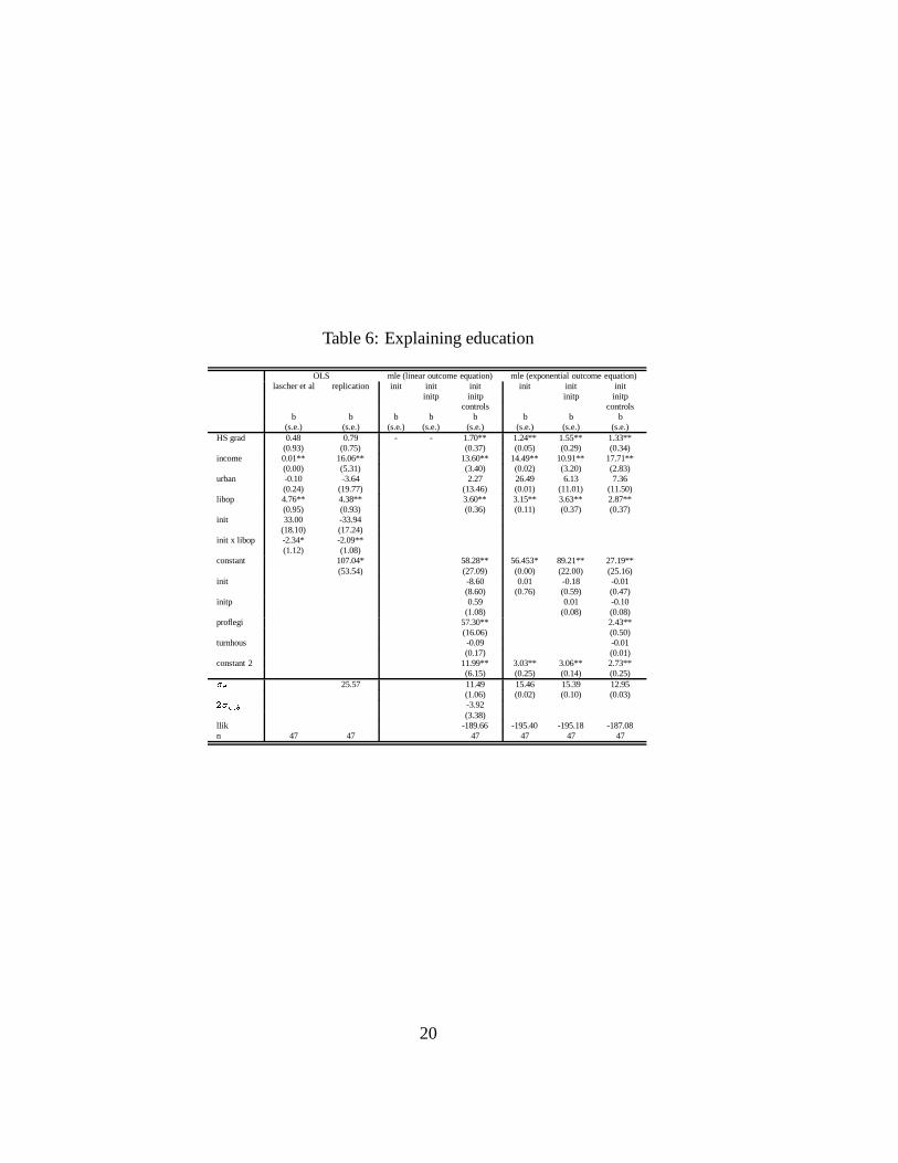
Table 6: Explaining education




HS grad 0.48 0.79 - - 1.70** 1.24** 1.55** 1.33**(0.93) (0.75) (0.37) (0.05) (0.29) (0.34)

income 0.01** 16.06** 13.60** 14.49** 10.91** 17.71**(0.00) (5.31) (3.40) (0.02) (3.20) (2.83)

urban -0.10 -3.64 2.27 26.49 6.13 7.36(0.24) (19.77) (13.46) (0.01) (11.01) (11.50)

libop 4.76** 4.38** 3.60** 3.15** 3.63** 2.87**(0.95) (0.93) (0.36) (0.11) (0.37) (0.37)

init 33.00 -33.94(18.10) (17.24)

init x libop -2.34* -2.09**(1.12) (1.08)

constant 107.04* 58.28** 56.453* 89.21** 27.19**(53.54) (27.09) (0.00) (22.00) (25.16)

init -8.60 0.01 -0.18 -0.01(8.60) (0.76) (0.59) (0.47)

initp 0.59 0.01 -0.10(1.08) (0.08) (0.08)

proflegi 57.30** 2.43**(16.06) (0.50)

turnhous -0.09 -0.01(0.17) (0.01)

constant 2 11.99** 3.03** 3.06** 2.73**(6.15) (0.25) (0.14) (0.25)

�� 25.57 11.49 15.46 15.39 12.95(1.06) (0.02) (0.10) (0.03)� � �� -3.92(3.38)

llik -189.66 -195.40 -195.18 -187.08n 47 47 47 47 47 47

20

Table 7: Explaining ERA




HS grad 0.15** 0.12** -0.01 -0.01 -0.01 0.11** -0.01 -0.02**(0.07) (0.06) (0.01) (0.01) (0.01) (0.03) (0.01) (0.01)

income 0.00 0.23 0.00 -0.10 0.00 -0.36 -0.10 0.19*(0.00) (0.40) (0.10) (0.10) (0.10) (0.30) (0.17) (0.14)

urban -0.03** -3.41** 0.83** 1.01** 0.83** 0.14 1.49** -0.26(0.02) (1.51) (0.49) (0.51) (0.58) (0.98) (0.61) (0.68)

libop 0.27** 0.24** 0.00 0.00 0.00 0.26** -0.00 -0.03**(0.07) (0.07) (0.02) (0.02) (0.02) (0.04) (0.02) (0.02)

init -2.69** -2.52**(1.29) (1.31)

init x libop -0.08 -0.08(0.08) (0.08)

constant -0.63 3.37** 3.56** 2.78** 3.70** 3.42** 2.12**(4.08) (0.84) (0.87) (0.86) (1.88) (0.89) (1.04)

init -0.04 -0.52 -0.27 0.44** -0.41** -0.33**(0.15) (0.44) (0.26) (0.23) (0.20) (0.18)

initp 0.06 0.04 0.04* 0.02(0.05) (0.03) (0.02) (0.02)

proflegi 1.05 0.70(0.70) (0.25)

turnhous 0.00 0.00(0.00) (0.00)

constant 2 2.76** 2.82** 2.40** 0.38 1.08 0.95(0.15) (0.15) (0.24) (0.16) (0.04) (0.08)

� � 1.95 0.71 0.67 0.70 1.13 0.55 0.57(0.05) (0.05) (0.05) (0.00) (0.00) (0.00)� � �� 0.44 0.38 0.47(0.12) (0.13) (0.13)

llik -35.79 -35.07 -72.33 -38.98 -40.17n 47 47 47 47 47 47 47 47

21

Table 8: Explaining gambling




HS grad 1.77 -1.30 6.77** 1.42 1.50 6.35** 1.66 5.80**(3.65) (3.11) (1.76) (1.36) (1.42) (1.65) (1.37) (1.76)

income -0.01 11.05 -1.30 22.50** 20.40* -0.83 21.69* 1.23(0.01) (21.94) (13.10) (11.10) (11.50) (13.79) (11.83) (15.62)

urban 0.54 -34.26 27.08 -41.97 -33.66 19.53 -33.50 -6.50(0.96) (81.60) (50.22) (42.65) (41.56) (49.52) (43.69) (58.42)

libop 24.7** 23.65** 17.04** 7.88** 8.09** 17.32** 7.91** 16.05**(3.70) (3.83) (1.63) (1.65) (1.66) (1.69) (1.66) (1.76)

init -84.80 -67.89(71.10) (71.16)

init x libop -10.10** -9.83**(4.40) (4.44)

constant 570.06** 44.92 102.37 115.86 76.21 90.28 78.47(221.01) (124.15) (105.89) (114.29) (119.12) (109.08) (118.19)

init -10.60 -60.68* -45.67 -0.08 -0.55 -0.19(19.72) (35.14) (31.65) (0.22) (0.44) (0.57)

initp 3.07 0.91 0.03 0.00(4.12) (4.04) (0.05) (0.07)

proflegi -16.21 -0.29(59.73) (0.86)

turnhous -0.57 -0.01(0.65) (0.01)

constant 2 95.98** 126.39** 142.30** 4.54** 4.83** 4.86**(13.04) (12.10) (24.40) (0.14) (0.10) (0.29)

�� 105.54 57.54 59.24 58.19 62.97 54.12 62.16(4.22) (4.66) (4.56) (0.17) (0.14) (0.17)� � �� -11.30 10.23 8.59(14.92) (12.66) (12.52)

llik -260.92 -253.97 -253.85 -261.39 -254.28 -260.79n 47 47 47 47 47 47 47

22

Table 9: Explaining medicare




HS grad 0.22 0.32 0.03 -0.21 -0.19 0.24 0.43** -0.15(0.47) (0.40) (0.16) (0.17) (0.19) (0.27) (0.25) (0.17)

income 0.00 -1.41 2.80* 5.10** 3.30* 2.69* 3.98** 5.49**(0.00) (2.80) (1.50) (1.60) (1.90) (1.71) (1.93) (1.61)

urban 0.07 11.91 10.93* 8.04 14.09** 16.31** 1.44 0.42(0.12) (10.42) (5.63) (6.09) (6.19) (7.82) (8.19) (5.33)

libop 1.64** 1.87** 0.56** 0.42** 0.56** 1.31** 1.19** 0.48**(0.48) (0.49) (0.19) (0.20) (0.19) (0.21) (0.17) (0.19)

init -10.40 -11.34(9.20) (9.09)

init x libop -0.74 -0.76(0.57) (0.57)

constant 138.02** 104.77** 99.77** 111.35** 93.80** 77.61** 96.87**(28.23) (11.70) (12.19) (13.12) (13.87) (14.60) (12.72)

init -1.82 -10.48** -9.03** 0.07 -0.85** -1.14**(2.03) (4.36) (4.41) (0.17) (0.45) (0.38)

initp 1.18* 0.88 0.11** 0.14**(0.54) (0.59) (0.04) (0.04)

proflegi 10.80 0.67(7.17) (0.55)

turnhous -0.01 -0.00(0.08) (0.01)

constant 2 13.38** 13.75** 11.49** 2.44** 2.39** 2.51**(1.38) (1.41) (2.92) (0.12) (0.13) (0.23)

�� 13.48 5.01 5.79 5.88 6.98 7.24 6.28(0.48) (0.56) (0.53) (0.01) (0.01) (0.02)� � �� -2.73 -1.18 -0.99(1.49) (1.60) (1.63)

llik -155.90 -154.79 -154.15 -158.04 -159.75 -153.06n 47 47 47 47 47 47 47 47

23

Table 10: Explaining taxes




HS grad 0.18 0.22 0.02 0.01 - 0.11** -0.01 0.09*(0.14) (0.12) (0.05) (0.05) (0.04) (0.05) (0.06)

income 0.00 -0.70 0.30 0.40 -0.23 0.37 0.65*(0.00) (0.85) (0.50) (0.50) (0.48) (0.34) (0.52)

urban 0.00 2.36 2.18 1.29 0.21 0.18 -3.27**(0.04) (3.17) (1.55) (1.77) (1.80) (1.63) (1.98)

libop 0.37** 0.37** 0.33** 0.33** 0.37** 0.35** 0.35**(0.15) (0.15) (0.06) (0.06) (0.06) (0.05) (0.06)

init -3.37 -3.75(2.81) (2.77)

init x libop -0.16 -0.18(0.17) (0.17)

constant -7.31 -2.64 -2.61 -3.90 -0.08 -8.56**(8.59) (5.62) (5.50) (3.69) (2.00) (4.30)

init 0.21 -1.14 0.17 -0.62** -1.13**(0.65) (1.47) (0.21) (0.29) (0.60)

initp 0.19 0.10** 0.17**(0.19) (0.02) (0.06)

proflegi 0.26(0.84)

turnhous -0.01*(0.01)

constant 2 3.44** 3.42** 1.09** 1.22** 1.26**(0.43) (0.43) (0.15) (0.15) (0.24)

�� 4.10 1.61 1.62 2.28 2.15 2.12(0.18) (0.19) (0.00) (0.01) (0.01)� � � � � -0.94 -0.87(0.60) (0.61)

llik -103.24 -102.72 -105.35 -102.70 -101.97n 47 47 47 47 47 47 47

24

Table 11: Explaining summary policy index (zpolicy)




HS grad 0.04** 0.04** 0.02** -0.01 0.02** 0.01** 0.05**(0.02) (0.01) (0.01) (0.01) (0.01) (0.01) (0.01)

income 0.00 0.64 0.10** 0.30** 0.14** 0.17** 0.06(0.00) (0.10) (0.10) (0.10) (0.05) (0.06) (0.08)

urban 0.00 0.32 0.27 -0.03 0.39** 0.06 -0.34(0.00) (0.38) (0.20) (0.21) (0.20) (0.26) (0.35)

libop 0.11** 0.11** 0.11** 0.09** 0.10** 0.11** 0.08**(0.02) (0.02) (0.01) (0.01) (0.01) (0.01) (0.01)

init -0.51 -0.51(0.33) (0.33)

init x libop -0.03 -0.03(0.02) (0.02)

constant -1.72 -0.68 -0.30 -1.61** -0.95** 4.65(1.04) (0.55) (0.50) (0.39) (0.48) (9.30)

init 0.07 -0.38** 0.19 -0.39 -0.02(0.08) (0.15) (0.18) (0.38) (0.05)

initp 0.06** 0.08* 0.01(0.02) (0.04) (0.01)

proflegi -0.55** -0.26(0.31) (0.34)

turnhous -0.00 0.00(0.00) (0.00)

constant 2 0.39** 0.67** -0.96** -0.97** 2.03**(0.05) (0.12) (0.12) (0.13) (1.22)

�� 0.49 0.26 0.27 0.25 0.25 0.40(0.02) (0.02) (0.00) (0.00) (0.00)� � �� 0.00 0.07(0.07) (0.06)

llik -2.70 1.79 -1.41 -1.35 -23.11n 47 47 47 47 47 47 47

25

7 Conclusion

In the current discussion of the merits and drawbacks of direct legislation both in

the states and around the world, misguided generalizations often lead to erroneous

statements about the effect of direct legislation. Systematic studies of the effect of

direct legislation on policy outcomes (e.g., Matsusaka 1995 and 2000, Gerber (1996

and 1999), Kirchgassner, Feld and Savioz 1999, Feld and Matsusaka 2000, Gerber

and Hug 2001) come to more nuanced conclusions that journalistic assessments (e.g.,

Schrag 1998 and Broder 2000) or studies relying on case studies (e.g. Smith 1998).

But even among the more systematic studies it has often proved elusive to find

demonstrable effects of direct legislation on policy outcomes of the type we would ex-

pect from theory. In this paper I argued that the reason for this elusive quest is largely

attributable to faulty empirical models. Based on the basic implication of most theo-

retical models, I derived two empirical models which improve on the models currently

used by researchers trying to show that direct legislation has policy consequences.

More precisely, these models directly acknowledge the fact that the effect of direct

legislation is contingent on the preferences of at least the voters. Taking this into con-

sideration in the empirical models I employed in this paper, I was able to show that

results obtained by Lascher, Hagen and Rochlin (1996) are problematic, and do not

allow for the rejection of the theoretically derived hypothesis. More precisely, using

their dataset and replicating their analysis both with their empirical model and the ones

proposed here, I demonstrated that the improved empirical models yield results largely

in synch with theory. In addition, both empirical models proposed here yield largely

similar results, testifying to the robustness of the results discussed here.

This empirical investigation, however, is hardly sufficient to demonstrate the merits

of the empirical models proposed here. Future research has to show to what degree

the simplifying assumptions employed to derive the two empirical models affect the

properties of the estimates obtained with their help. Only Monte-Carlo simulations,

especially given the importance of small-sample properties, can yield answers to this

important question. Future will tell.

26

8 Appendix

Table 12 reports the descriptive statistics of the variables employed in this paper.

Table 12: Descriptive statistics

variable minimum mean maximum std dev NINIT direct legislation dummy 0 0.45 1 0.5 47INITP lowest signature requirement for initiative 0 3.28 15 4.12 47libop state ideology measure -28 -14.6 -0.81 7.3 47income mean income 1980 6.68 9.01 11.54 1.17 47HS grad percent of high school graduates 53 66.4 80 7.32 47urban percent of urban policy 0 0.53 0.93 0.25 47ADC80 87 241.36 400 83.45 47CONSUME2 4 13.57 21 3.85 47CRIMJUS2 -100 153.19 400 131.63 47EXPPUPIL 168 237.85 376 47.99 47ERABOLES 0 3.74 6 2.63 47GAMBLING 0 257.45 600 171.62 47MEDICAR2 100 125.94 159 17.7 47LOWRY2 -13 -3.45 7 4.67 47ZPOLICY -1.55 0 2.13 1 47TURNHOUS turnouver rate in state house 2 21.7 55 12.88 47PROFLEGI professionalization of legislature 0.04 0.22 0.66 0.15 47

27

References

Bartels, Larry M. 1991. Constituency Opinion and Congressional Policy Making: The

Reagan Defense Buildup. American Political Science Review. 85(2 June) 457-474.

Black, Duncan 1958. Theory of Committees and Elections. Cambridge: Cambridge

University Press.

Bowen, Howard R. 1943. The Interpretation of Voting in Allocation of Economic

Resources. Quarterly Journal of Economics. 58(1 (Nov)) 27-48.

Broder, David S. 2000. Democracy Derailed. Initiative Campaigns and the Power of

Money. New York: James H. Silberman Book/Harcourt.

Camobreco, John F. 1998. Preferences, Fiscal Policies, and the Initiative Process.

Journal of Politics. 60(AUG 3) 819-829.

Chicoine, D. L.; Walzer, N.; Deller, S. C. 1989. Representative vs. Direct Democracy

and Government Spending in a Median Voter Model. Public Finance. 44(2) 225-

236.

Council of State Governments 1935-. The Book of the States. Lexington: Council of

State Governments.

Cronin, Thomas E. 1989. Direct Democracy. The Politics of Initiative, Referendum

and Recall. Cambridge: Harvard University Press.

Erikson, Robert S.; Wright, Gerald C.; McIver, John P. 1993. Statehouse Democracy:

Public Opinion and Policy in the American States. New York: Cambridge Univer-

sity Press.

Feld, Lars P.; Matsusaka, John G. 2000. Budget Referendums and Government Spend-

ing: Evidence from Swiss Cantons. St.Gallen: SIASR, University of St.Gallen.

Gerber, Elisabeth R. 1996. Legislative Response to the Threat of Popular Initiatives.

American Journal of Political Science. 40(1) 99-128.

Gerber, Elisabeth R. 1999. The Populist Paradox: Interest Group Influence and the

Promise of Direct Legislation. Princeton: Princeton University Press.

Gerber, Elisabeth R.; Hug, Simon (forthcoming 2001). Legislative Responses to Di-

rect Legislation. in Mendelsohn, Matthew; Parkin, Andrew (eds.) Referendum

Democracy. Citizens, Elites, and Deliberation in Referendum Campaigns. New

York: Palgrave.

Gerber, Elisabeth R.; Hug, Simon 2001. Minority Rights and Direct Legislation. The-

ory, Methods, and Evidence. La Jolla: Department of Political Science, University

28

of California, San Diego.

Holcombe, Randall G. 1989. The Median Voter Model in Public Choice Theory. Pub-

lic Choice. 61(2) 115-126.

Hug, Simon 1999. Occurrence and Policy Consequences of Referendums. A Theo-

retical Model and Empirical Evidence. La Jolla: Department of Political Science,

University of California, San Diego.

Hug, Simon; Tsebelis, George 2000. Veto Players and Referendums around the World.

Austin: University of Texas, Department of Government.

Key, V. 0. Jr.; Crouch, Winston W. 1939. The Initiative and the Referendum in Cali-

fornia. Berkeley : University of California Press.

Kirchgassner, Gebhard; Feld, Lars P.; Savioz, Marcel R. 1999. Die direkte Demokratie

der Schweiz: Modern, erfolgreich, entwicklungs- und exportfahig. Basel: Helbing

und Lichtenhahn.

Lascher, Edward L.; Hagen, Michael G.; Rochlin, Steven A. 1996. Gun Behind the

Door - Ballot Initiatives, State Policies and Public Opinion. Journal of Politics.

58(3) 760-775.

Matsusaka, John G. 1995. Fiscal Effects of the Voter Initiative: Evidence from the last

30 Years. Journal of Political Economy. 103(3) 587-623.

Matsusaka, John G. 2000. Fiscal Effects of the Voter Initiative in the First Half of the

Twentieth Century. Journal of Law and Economics. 43 (OCT 2) 619-644.

Matsusaka, John G. forthcoming. Problems with a Methodology Used to Test Whether

Policy Is More or Less Responsive to Public Opinion in States with Voter Intiatives.

Journal of Politics.

Matsusaka, John G.; McCarty, Nolan M. 1998. Political Resource Allocation: The

Benefits and Costs of Voter Initiatives. Los Angeles: University of Southern Cali-

fornia, Marshall School of Business.

Moser, Peter 1996. Why is Swiss Politics so Stable? Zeitschrift fur Volkswirtschaft

und Statistik. 132(1) 31-60.

Pommerehne, Werner W. 1978a. Institutional Approaches to Public Expenditure: Em-

pirical Evidence from Swiss Municipalities. Journal of Public Economics. 9 255-

280.

Pommerehne, Werner W. 1978b. Politisch-okonomisches Modell der direkten and

reprasentativen Demokratie. in Helmstadter, Ernst (ed.) Neuere Entwicklungen

in der Wirtschaftswissenschaft. Berlin: Duncker und Humblot. pp. 569-589.

29

Romer, Thomas; Rosenthal, Howard 1979. The Elusive Median Voter. Journal of

Public Economics. 12 143-170.

Santoro, Wayne A.; McGuire, Gail M. 1997. Social Movement Insiders: The Impact

of Institutional Activists on Affirmative Action and Comparable Worth Policies.

Social Problems. 44(NOV 4) 503-519.

Schrag, Peter 1998. Paradise Lost: California’s Experience, America’s Future . New

York: New Press.

Smith, Daniel A. 1998. Tax Crusaders and the Politics of Direct Democracy . New

York: Routledge.

Squire, Peverill 1992. Legislative Professionalization and Membership Diversity in

State Legislatures. Legislative Studies Quarterly. 17(FEB 1) 69-79.

Steunenberg, Bernard 1992. Referendum, Initiative, and Veto Power. Kyklos. 45(4)

501-529.

Tsebelis, George 2000. Veto Players in Political Analysis. Governance. 13(3 October)

441-474.

pcdls/simon/ February 19, 2001

30

Documents

Policy Consequences of Direct Legislation in the … Consequences of Direct Legislation in the States Theory, Empirical Models and Evidence ... Phil Paolino, and