HAL Id: tel-00577887https://tel.archives-ouvertes.fr/tel-00577887

Submitted on 17 Mar 2011

HAL is a multi-disciplinary open accessarchive for the deposit and dissemination of sci-entific research documents, whether they are pub-lished or not. The documents may come fromteaching and research institutions in France orabroad, or from public or private research centers.

L’archive ouverte pluridisciplinaire HAL, estdestinée au dépôt et à la diffusion de documentsscientifiques de niveau recherche, publiés ou non,émanant des établissements d’enseignement et derecherche français ou étrangers, des laboratoirespublics ou privés.

Polarization of surface waves : characterization,inversion and application to seismic hazard assessment

Manuel Hobiger

To cite this version:Manuel Hobiger. Polarization of surface waves : characterization, inversion and application toseismic hazard assessment. Earth Sciences. Université de Grenoble, 2011. English. <NNT :2011GRENU005>. <tel-00577887>

THÈSE Pour obtenir le grade de

DOCTEUR DE L’UNIVERSITÉ DE GRENOBLE Spécialité : Sciences de la Terre, de l’Univers et de l’Environnement Arrêté ministériel : 7 août 2006 Présentée par

Manuel HOBIGER Thèse dirigée par Pierre-Yves BARD et codirigée par Cécile CORNOU et Nicolas LE BIHAN préparée au sein de l’Institut des Sciences de la Terre (ISTerre) dans l'École Doctorale Terre, Univers, Environnement

Polarisation des ondes de surface : Caractérisation, inversion et application à l’étude de l’aléa sismique Thèse soutenue publiquement le 13 janvier 2011, devant le jury composé de :

Michel CAMPILLO ISTerre, Grenoble, Président Donat FÄH ETH Zürich, Rapporteur Pascal LARZABAL ENS Cachan, Rapporteur Matthias OHRNBERGER Universität Potsdam, Examinateur Ulrich WEGLER BGR, Hannover, Examinateur Pierre-Yves BARD ISTerre, Grenoble, Directeur de thèse Cécile CORNOU ISTerre, Grenoble, Directrice de thèse Nicolas LE BIHAN GIPSA-Lab, Grenoble, Directeur de thèse

Polarization of surface waves:

Characterization, inversion and

application to seismic hazard assessment

Polarisation des ondes de surface :Caractérisation, inversion et

application à l’étude de l’aléa sismique

5

Summary

The estimation of site effects is an important task in seismic hazard assessment. Inorder to understand and estimate these site effects, the local soil structure as well as thecomposition (body/surface waves, Love/Rayleigh waves) and properties of the wavefield have to be investigated. Instead of using expensive methods such as borehole mea-surements or reflection or refraction seismics, these properties can be investigated usingsurface waves. The two most important types of seismic surface waves are Love andRayleigh waves. These waves exhibit dispersion curves which are directly linked to thesoil structure. Furthermore, the ellipticity, a parameter describing the elliptical motion ofRayleigh waves as a function of frequency, is also linked to the soil structure. In order toidentify and extract different wave types, their respective polarization parameters haveto be characterized.

In a first part of this work, new methods allowing the determination of the polarizationparameters of seismic surface waves are developed. Two methods, DELFI and RayDec,estimate the ellipticity of Rayleigh waves using the three-dimensional record of a singleseismic station. The first method tries to directly fit ellipses to parts of the signal, whereasthe second one uses statistical properties to effectively suppress other wave types thanRayleigh waves. A third newly developed method, MUSIQUE, is the combination ofthe established MUSIC algorithm with a version using quaternions, an example of hy-percomplex numbers. MUSIQUE uses seismic array recordings to discriminate betweenLove and Rayleigh waves, estimate the related dispersion curves and the Rayleigh waveellipticity.

In the second part of the work, the new methods are applied to real data measurements.A theoretical investigation of the inversion of ellipticity curves shows that the right flankof the ellipticity peak and the peak frequency carry the important information on thesoil structure. However, as the ellipticity curve is not unique, additional information,e.g. small-scale SPAC or MASW measurements, have to be added to the inversion. Ina second step, ellipticity curves estimated by RayDec on real data measurements areinverted jointly with SPAC measurements. For the 14 investigated sites, the inversionresults are in good agreement with direct dispersion curve measurements. Furthermore,the ellipticity inversion could help in identifying the correct Rayleigh wave modes. Inthe last chapter, the seismological wave field generated by 22 earthquakes and recordedwith a dense seismic array in the Santa Clara Valley, California, is investigated usingMUSIQUE. Large amounts of scattered Love waves arriving from southern directions arefound. Furthermore, the estimated energy repartition between Love and Rayleigh wavesfor the different events is rather heterogeneous. Finally, combining the information ofall earthquakes, the dispersion curves for both the fundamental and the first harmonicLove wave modes are retrieved. For the fundamental Rayleigh wave mode, neither thedispersion nor the ellipticity curve can be found, but for the first harmonic Rayleighwave mode both properties are identified.

7

Résumé

L’analyse des effets de site joue un rôle décisif pour l’estimation de l’aléa sismique. Afin decomprendre et de quantifier ces effets de site, il faut étudier la structure locale du sol ainsi quela composition (ondes de volume/surface, ondes de Love/Rayleigh) et les propriétés du champd’ondes. Au lieu de techniques coûteuses comme des mesures par forage ou la sismique parréflexion ou réfraction, ces propriétés peuvent être analysées en utilisant les ondes de surface.Les deux types d’ondes de surface de loin les plus importants en sismologie sont les ondes deLove et de Rayleigh. Ces ondes sont caractérisées par des courbes de dispersion directement liéesà la structure du sol. En outre, l’ellipticité, un paramètre décrivant le mouvement elliptique desondes de Rayleigh en fonction de la fréquence, est aussi liée à la structure du sol. Afin d’identifieret d’extraire les différents types d’ondes, leurs paramètres de polarisation doivent être caractérisés.

Dans la première partie de ce manuscrit, de nouvelles méthodes permettant la déterminationdes paramètres de polarisation des différents types d’ondes de surface sont développées. Deuxde ces méthodes, DELFI et RayDec, évaluent l’ellipticité des ondes de Rayleigh à partir del’enregistrement à trois composantes d’un seul capteur sismique. La première de ces méth-odes essaie d’ajuster directement des ellipses à des parties du signal, tandis que la deuxièmeréprime tout type d’onde sauf les ondes de Rayleigh en exploitant des propriétés statistiques.Une troisième nouvelle méthode, MUSIQUE, représente la combinaison de l’algorithme MU-SIC avec une version utilisant les quaternions, des nombres hypercomplexes de dimension 4.Cette méthode utilise les enregistrements de réseaux sismiques pour distinguer ondes de Love etondes de Rayleigh, estimer les courbes de dispersion associées et l’ellipticité des ondes de Rayleigh.

La deuxième partie du manuscrit est dédiée à l’application des nouvelles méthodes sur desdonnées réelles. Une ’etude théorique des inversions de courbes d’ellipticité montre que le flancdroit du pic d’ellipticité et la fréquence du pic comportent toutes les informations nécessairespour caractériser la structure du sol. Cependant, la courbe d’ellipticité n’étant pas unique, desinformations supplémentaires sur la vitesse des ondes de cisaillement de la proche surface doiventêtre inclues dans le processus d’inversion. Une seconde étude s’intéresse à l’inversion conjointede courbes d’ellipticité mesurés par RayDec avec des mesures d’autocorrélation spatiale surdes données réelles acquises dans différents sites en Europe. Sur les 14 sites ainsi analysés, lesrésultats de l’inversion sont en bon accord avec les mesures directes de courbes de dispersion.Par ailleurs, la méthode montre son potentiel à discriminer les différents modes de Rayleighobservés. Dans le dernier chapitre, le champ d’ondes issu de l’enregistrement de séismes parun réseau de capteurs sismiques dans la vallée de Santa Clara en Californie est analysé parMUSIQUE. De grandes quantités d’ondes de Love diffusées arrivant de directions méridionalessont identifiées. En outre, la répartition entre ondes de Love et ondes de Rayleigh varie fortementpour les différents évènements. Finalement, en combinant les informations de tous les séismes,les courbes de dispersion pour le mode fondamental et le premier mode harmonique des ondesde Love sont identifiées. Pour le mode fondamental des ondes de Rayleigh, ni la courbe dedispersion ni la courbe d’ellipticité ne sont trouvées, tandis que pour le premier mode harmonique,les deux propriétés sont identifiées.

9

Acknowledgments

In the following, I would like to express my gratitude to those without whom this workcould not have been done.

Trois directeurs de thèse, Cécile, Pierre-Yves et Nicolas, m’ont encadré pendant cestrois ans. Profitant ainsi de la combinaison de leurs savoir-faire et de trois points devue différents, c’était une grande chance pour moi. Merci de m’avoir proposé ce sujetintéressant et d’avoir toujours été disponible à aider et donner de bons conseils.

I would also like to thank Donat Fäh and Pascal Larzabal for having willingly acceptedto review this work and Michel Campillo, Matthias Ohrnberger and Ulrich Wegler forhaving consented to be part of the jury.

It was a big opportunity to use the abundance of data measured during the Neriesproject. Thanks to all who participated in these measurements. I would also like to thankFlorence, Brigitte and Giuseppe for their help and good discussions and Marc for hisavailability and support with geopsy and dinver. It was also a big pleasure to work withAlekos and Nikos, especially during the field campaign in Greece. I will also keep goodmemories of the measurements with Seiji in Cadarache and La Tronche.

Another thank goes to Arthur Frankel and David Carter who willingly provided the dataof the San Jose seismic array and Arthur Rodgers who helped with good discussions andthe Bay Area model to analyze the data.

Merci aussi à Cécile (encore une fois) et Manu pour m’avoir accueilli, en 2005, pour lestage de master et m’avoir donné l’envie pour la sismologie. Ce stage était finalement laraison pour laquelle je suis revenu au LGIT pour passer la thèse.

C’était toujours un vrai plaisir de travailler au LGIT qui m’est devenu comme une deux-ième maison. Un grand merci aux autres étudiants pour avoir rendu le travail le plusagreáble possible, mais aussi pour les différentes escapades qu’on a faites, les balades enmontagne, le ski ou les nuits à regarder les étoiles.

Merci à l’équipe de foot du LGIT, c’était un plaisir et un honneur de représenter lescouleurs du LGIT sur les terrains de foot, même si le succès n’était pas toujours de notrecôté.

Enfin, merci aussi à ceux dont le travail reste assez souvent inaperçu, mais qui sontindispensables pour le bon déroulement d’une thèse : les équipes informatique et admin-istrative et l’Ecole Doctorale.

Ein besonderer Dank geht schließlich an meine Eltern, auf deren Unterstützung ich michauf diesem langen Weg immer verlassen konnte und die mir stets mit Rat und Tat zurSeite standen.

Contents

Summary 5

Résumé 7

Contents 11

Introduction 21

Thesis outline 29

I Theory 31

1 Properties of seismic waves 331.1 Wave equation . . . . . . . . . . . . . . . . . . . . . . . . . . . . . . . . . . . 341.2 Body waves . . . . . . . . . . . . . . . . . . . . . . . . . . . . . . . . . . . . 341.3 Surface waves . . . . . . . . . . . . . . . . . . . . . . . . . . . . . . . . . . . 35

1.3.1 Love waves . . . . . . . . . . . . . . . . . . . . . . . . . . . . . . . . 351.3.2 Rayleigh waves . . . . . . . . . . . . . . . . . . . . . . . . . . . . . . 36

1.4 Conclusion . . . . . . . . . . . . . . . . . . . . . . . . . . . . . . . . . . . . . 38

11

12 CONTENTS

2 Single-sensor methods to estimate the polarization of seismic waves 392.1 Introduction . . . . . . . . . . . . . . . . . . . . . . . . . . . . . . . . . . . . 402.2 Overview of existing methods . . . . . . . . . . . . . . . . . . . . . . . . . . 41

2.2.1 Rectilinear and planar polarization filters . . . . . . . . . . . . . . . 412.2.1.1 Rectilinear polarization filter . . . . . . . . . . . . . . . . . 412.2.1.2 Planar polarization filter . . . . . . . . . . . . . . . . . . . 42

2.2.2 Polarization analysis using the analytic signal . . . . . . . . . . . . 432.2.3 H/V . . . . . . . . . . . . . . . . . . . . . . . . . . . . . . . . . . . . 44

2.3 DELFI . . . . . . . . . . . . . . . . . . . . . . . . . . . . . . . . . . . . . . . . 452.3.1 Plane detection . . . . . . . . . . . . . . . . . . . . . . . . . . . . . . 452.3.2 Ellipse fitting . . . . . . . . . . . . . . . . . . . . . . . . . . . . . . . 472.3.3 Free parameters . . . . . . . . . . . . . . . . . . . . . . . . . . . . . . 49

2.4 RayDec . . . . . . . . . . . . . . . . . . . . . . . . . . . . . . . . . . . . . . . 512.4.1 Abstract . . . . . . . . . . . . . . . . . . . . . . . . . . . . . . . . . . 512.4.2 Introduction . . . . . . . . . . . . . . . . . . . . . . . . . . . . . . . . 512.4.3 Methodology . . . . . . . . . . . . . . . . . . . . . . . . . . . . . . . 532.4.4 Application to synthetic noise . . . . . . . . . . . . . . . . . . . . . . 55

2.4.4.1 Influence of the parameters of the method . . . . . . . . . 562.4.4.2 Minimum required signal length and temporal stability

of the results . . . . . . . . . . . . . . . . . . . . . . . . . . 562.4.4.3 Results for the models N101, N103 and N104 . . . . . . . 57

2.4.5 Application to real noise data . . . . . . . . . . . . . . . . . . . . . . 592.4.6 Conclusion . . . . . . . . . . . . . . . . . . . . . . . . . . . . . . . . 59

2.5 Conclusion . . . . . . . . . . . . . . . . . . . . . . . . . . . . . . . . . . . . . 60

CONTENTS 13

3 Characterization of seismic waves using arrays of sensors 613.1 Introduction . . . . . . . . . . . . . . . . . . . . . . . . . . . . . . . . . . . . 623.2 Delay-and-sum beamforming . . . . . . . . . . . . . . . . . . . . . . . . . . 643.3 Frequency-wavenumber analysis . . . . . . . . . . . . . . . . . . . . . . . . 65

3.3.1 Resolution limits of seismic arrays . . . . . . . . . . . . . . . . . . . 663.4 MUSIC . . . . . . . . . . . . . . . . . . . . . . . . . . . . . . . . . . . . . . . 673.5 Spatial autocorrelation technique (SPAC) . . . . . . . . . . . . . . . . . . . 69

3.5.1 Vertical component . . . . . . . . . . . . . . . . . . . . . . . . . . . . 693.5.2 Horizontal components . . . . . . . . . . . . . . . . . . . . . . . . . 723.5.3 Rayleigh and Love waves . . . . . . . . . . . . . . . . . . . . . . . . 743.5.4 Applying the SPAC method . . . . . . . . . . . . . . . . . . . . . . . 76

3.5.4.1 The Bessel functions . . . . . . . . . . . . . . . . . . . . . . 763.5.4.2 Practical problems . . . . . . . . . . . . . . . . . . . . . . . 763.5.4.3 Mathematical considerations relating to the number of

seismic stations . . . . . . . . . . . . . . . . . . . . . . . . 793.5.5 Modified SPAC method (M-SPAC) . . . . . . . . . . . . . . . . . . . 82

3.5.5.1 Vertical component . . . . . . . . . . . . . . . . . . . . . . 823.5.5.2 Horizontal components . . . . . . . . . . . . . . . . . . . . 83

3.5.6 Two-sites SPAC method (2s-SPAC) . . . . . . . . . . . . . . . . . . . 853.5.7 Application of 2s-SPAC to real data measurements . . . . . . . . . 85

3.5.7.1 Location near the school . . . . . . . . . . . . . . . . . . . 863.5.7.2 Location near the hospital . . . . . . . . . . . . . . . . . . 88

3.6 Conclusion . . . . . . . . . . . . . . . . . . . . . . . . . . . . . . . . . . . . . 92

14 CONTENTS

4 Advanced seismic array methods using hypercomplex numbers 934.1 Introduction . . . . . . . . . . . . . . . . . . . . . . . . . . . . . . . . . . . . 944.2 Quaternions . . . . . . . . . . . . . . . . . . . . . . . . . . . . . . . . . . . . 95

4.2.1 Definition . . . . . . . . . . . . . . . . . . . . . . . . . . . . . . . . . 954.2.2 Properties . . . . . . . . . . . . . . . . . . . . . . . . . . . . . . . . . 964.2.3 Cayley-Dickson representation . . . . . . . . . . . . . . . . . . . . . 974.2.4 Quaternion vectors . . . . . . . . . . . . . . . . . . . . . . . . . . . . 974.2.5 Quaternion matrices . . . . . . . . . . . . . . . . . . . . . . . . . . . 98

4.3 Biquaternions . . . . . . . . . . . . . . . . . . . . . . . . . . . . . . . . . . . 1004.3.1 Definition . . . . . . . . . . . . . . . . . . . . . . . . . . . . . . . . . 1004.3.2 Properties . . . . . . . . . . . . . . . . . . . . . . . . . . . . . . . . . 1004.3.3 Biquaternion vectors . . . . . . . . . . . . . . . . . . . . . . . . . . . 1014.3.4 Biquaternion matrices . . . . . . . . . . . . . . . . . . . . . . . . . . 102

4.4 Quaternion-MUSIC . . . . . . . . . . . . . . . . . . . . . . . . . . . . . . . . 1044.4.1 Methodology . . . . . . . . . . . . . . . . . . . . . . . . . . . . . . . 1044.4.2 Polarization parameter identification for known wave vector . . . 106

4.5 Biquaternion-MUSIC . . . . . . . . . . . . . . . . . . . . . . . . . . . . . . . 1094.5.1 Methodology . . . . . . . . . . . . . . . . . . . . . . . . . . . . . . . 1094.5.2 Polarization parameter identification for known wave vector . . . 110

4.5.2.1 Case of identical signals for all three components . . . . . 1134.5.2.2 Case of identical signals for two components . . . . . . . 1144.5.2.3 Case of two-dimensional signals . . . . . . . . . . . . . . . 115

4.6 MUSIQUE . . . . . . . . . . . . . . . . . . . . . . . . . . . . . . . . . . . . . 1174.6.1 Estimation of the wave vector by MUSIC . . . . . . . . . . . . . . . 1174.6.2 Estimation of the polarization parameters by quaternion-MUSIC . 1204.6.3 Assembling the results . . . . . . . . . . . . . . . . . . . . . . . . . . 121

4.7 Conclusion . . . . . . . . . . . . . . . . . . . . . . . . . . . . . . . . . . . . . 122

CONTENTS 15

5 Tests on synthetic data 1235.1 Introduction . . . . . . . . . . . . . . . . . . . . . . . . . . . . . . . . . . . . 1245.2 Influence of the signal-to-noise ratio . . . . . . . . . . . . . . . . . . . . . . 125

5.2.1 Signal generation . . . . . . . . . . . . . . . . . . . . . . . . . . . . . 1255.2.2 Analysis results . . . . . . . . . . . . . . . . . . . . . . . . . . . . . . 1275.2.3 Discussion of the results . . . . . . . . . . . . . . . . . . . . . . . . . 130

5.3 Tests on a theoretical dispersive signal . . . . . . . . . . . . . . . . . . . . . 1325.3.1 Signal generation . . . . . . . . . . . . . . . . . . . . . . . . . . . . . 1325.3.2 Analysis results . . . . . . . . . . . . . . . . . . . . . . . . . . . . . . 134

5.3.2.1 Single-sensor ellipticity estimation . . . . . . . . . . . . . 1345.3.2.2 MUSIQUE . . . . . . . . . . . . . . . . . . . . . . . . . . . 136

5.4 Tests on simulated seismic signals . . . . . . . . . . . . . . . . . . . . . . . 1405.4.1 Signal generation . . . . . . . . . . . . . . . . . . . . . . . . . . . . . 1405.4.2 Analysis results - Noise with a principal azimuth . . . . . . . . . . 142

5.4.2.1 Signals . . . . . . . . . . . . . . . . . . . . . . . . . . . . . 1425.4.2.2 Single-sensor ellipticity estimation . . . . . . . . . . . . . 1435.4.2.3 MUSIQUE . . . . . . . . . . . . . . . . . . . . . . . . . . . 145

5.4.3 Analysis results - Random noise source distribution . . . . . . . . . 1485.4.3.1 Signals . . . . . . . . . . . . . . . . . . . . . . . . . . . . . 1485.4.3.2 Single-sensor ellipticity estimation . . . . . . . . . . . . . 1495.4.3.3 MUSIQUE . . . . . . . . . . . . . . . . . . . . . . . . . . . 151

5.5 Conclusion . . . . . . . . . . . . . . . . . . . . . . . . . . . . . . . . . . . . . 154

16 CONTENTS

II Application 157

6 Inversion of ellipticity curves - Theoretical aspects 1596.1 Abstract . . . . . . . . . . . . . . . . . . . . . . . . . . . . . . . . . . . . . . 1606.2 Introduction . . . . . . . . . . . . . . . . . . . . . . . . . . . . . . . . . . . . 1606.3 Inversion algorithm . . . . . . . . . . . . . . . . . . . . . . . . . . . . . . . . 1636.4 Tests on theoretical data . . . . . . . . . . . . . . . . . . . . . . . . . . . . . 163

6.4.1 Model parameters . . . . . . . . . . . . . . . . . . . . . . . . . . . . 1646.4.2 Goodness of the inversion results . . . . . . . . . . . . . . . . . . . . 1646.4.3 Fixing the shear wave velocity at the surface

by spatial autocorrelation curves . . . . . . . . . . . . . . . . . . . . 1666.4.4 Which parts of the ellipticity curve are necessary

for the inversion process? . . . . . . . . . . . . . . . . . . . . . . . . 1686.4.4.1 Model with a singularity in the ellipticity curve . . . . . . 1686.4.4.2 Model without a singularity in the ellipticity curve . . . . 1736.4.4.3 Joint inversion of dispersion and ellipticity curves . . . . 175

6.4.5 Inversion of erroneous ellipticity curves . . . . . . . . . . . . . . . . 1776.4.5.1 Ellipticity misestimation by a constant factor . . . . . . . 1786.4.5.2 Frequency-dependent ellipticity misestimation . . . . . . 181

6.5 Conclusion . . . . . . . . . . . . . . . . . . . . . . . . . . . . . . . . . . . . . 184

CONTENTS 17

7 Inversion of ellipticity curves - Application to real data measurements 1857.1 Abstract . . . . . . . . . . . . . . . . . . . . . . . . . . . . . . . . . . . . . . 1867.2 Introduction . . . . . . . . . . . . . . . . . . . . . . . . . . . . . . . . . . . . 1867.3 Measurement methodology . . . . . . . . . . . . . . . . . . . . . . . . . . . 188

7.3.1 Ellipticity measurements . . . . . . . . . . . . . . . . . . . . . . . . 1887.3.2 Spatial autocorrelation measurements . . . . . . . . . . . . . . . . . 188

7.4 Inversion algorithm . . . . . . . . . . . . . . . . . . . . . . . . . . . . . . . . 1907.4.1 Goodness of the inversion results . . . . . . . . . . . . . . . . . . . . 1907.4.2 Inversion strategy . . . . . . . . . . . . . . . . . . . . . . . . . . . . 192

7.5 Application to real data measurements . . . . . . . . . . . . . . . . . . . . . 1937.5.1 Models with clear ellipticity peak . . . . . . . . . . . . . . . . . . . 196

7.5.1.1 Volvi . . . . . . . . . . . . . . . . . . . . . . . . . . . . . . . 1967.5.1.2 Nestos . . . . . . . . . . . . . . . . . . . . . . . . . . . . . . 1997.5.1.3 Colfiorito . . . . . . . . . . . . . . . . . . . . . . . . . . . . 201

7.5.2 Sites without clear ellipticity peak . . . . . . . . . . . . . . . . . . . 2047.5.2.1 Aigio . . . . . . . . . . . . . . . . . . . . . . . . . . . . . . 2047.5.2.2 Korinthos . . . . . . . . . . . . . . . . . . . . . . . . . . . . 206

7.5.3 Inversion results for the other sites . . . . . . . . . . . . . . . . . . . 2097.6 Overview of the results for all 14 sites . . . . . . . . . . . . . . . . . . . . . 211

7.6.1 Dispersion curves . . . . . . . . . . . . . . . . . . . . . . . . . . . . . 2117.6.2 Vs30 values . . . . . . . . . . . . . . . . . . . . . . . . . . . . . . . . 212

7.7 Conclusion . . . . . . . . . . . . . . . . . . . . . . . . . . . . . . . . . . . . . 2137.8 Appendix:

Inversion results for the other sites in detail . . . . . . . . . . . . . . . . . . 2157.8.1 Benevento . . . . . . . . . . . . . . . . . . . . . . . . . . . . . . . . . 2157.8.2 Bolu . . . . . . . . . . . . . . . . . . . . . . . . . . . . . . . . . . . . 2187.8.3 Buia . . . . . . . . . . . . . . . . . . . . . . . . . . . . . . . . . . . . 2207.8.4 Düzce . . . . . . . . . . . . . . . . . . . . . . . . . . . . . . . . . . . 2227.8.5 Forlì . . . . . . . . . . . . . . . . . . . . . . . . . . . . . . . . . . . . 2247.8.6 Knidi . . . . . . . . . . . . . . . . . . . . . . . . . . . . . . . . . . . . 2277.8.7 Norcia . . . . . . . . . . . . . . . . . . . . . . . . . . . . . . . . . . . 2307.8.8 Sakarya . . . . . . . . . . . . . . . . . . . . . . . . . . . . . . . . . . 2327.8.9 Sturno . . . . . . . . . . . . . . . . . . . . . . . . . . . . . . . . . . . 234

18 CONTENTS

8 Investigation of the seismological wave field: Earthquake array measurementsin California 2378.1 Introduction . . . . . . . . . . . . . . . . . . . . . . . . . . . . . . . . . . . . 2388.2 Array setup and basin model . . . . . . . . . . . . . . . . . . . . . . . . . . 2398.3 Database . . . . . . . . . . . . . . . . . . . . . . . . . . . . . . . . . . . . . . 2428.4 Data processing . . . . . . . . . . . . . . . . . . . . . . . . . . . . . . . . . . 2448.5 Azimuthal energy distribution . . . . . . . . . . . . . . . . . . . . . . . . . 245

8.5.1 Comparison between the the early and late signals . . . . . . . . . 2458.5.1.1 Event 1 . . . . . . . . . . . . . . . . . . . . . . . . . . . . . 2458.5.1.2 Event 3 . . . . . . . . . . . . . . . . . . . . . . . . . . . . . 2468.5.1.3 Event 5 . . . . . . . . . . . . . . . . . . . . . . . . . . . . . 2468.5.1.4 Event 6 . . . . . . . . . . . . . . . . . . . . . . . . . . . . . 247

8.5.2 Temporal Love wave azimuth evolution . . . . . . . . . . . . . . . . 2528.5.3 Results for the other events . . . . . . . . . . . . . . . . . . . . . . . 254

8.5.3.1 Events 4 and 22 . . . . . . . . . . . . . . . . . . . . . . . . 2548.5.3.2 Events 13-16 and 18-21 . . . . . . . . . . . . . . . . . . . . 2548.5.3.3 Events 7, 8 and 9 . . . . . . . . . . . . . . . . . . . . . . . . 2548.5.3.4 Events 2 . . . . . . . . . . . . . . . . . . . . . . . . . . . . . 2558.5.3.5 Events 10/12, 11 and 17 . . . . . . . . . . . . . . . . . . . . 255

8.5.4 Summary . . . . . . . . . . . . . . . . . . . . . . . . . . . . . . . . . 2558.6 Energy repartition between Love and Rayleigh waves . . . . . . . . . . . . 2628.7 Dispersion curves . . . . . . . . . . . . . . . . . . . . . . . . . . . . . . . . . 2668.8 Ellipticity curves . . . . . . . . . . . . . . . . . . . . . . . . . . . . . . . . . 2698.9 Conclusion . . . . . . . . . . . . . . . . . . . . . . . . . . . . . . . . . . . . . 271

CONTENTS 19

Conclusion 275

A Appendix: EUSIPCO paper 283A.1 Abstract . . . . . . . . . . . . . . . . . . . . . . . . . . . . . . . . . . . . . . 284A.2 Introduction . . . . . . . . . . . . . . . . . . . . . . . . . . . . . . . . . . . . 284A.3 Rayleigh wave ellipticity in seismology . . . . . . . . . . . . . . . . . . . . 285

A.3.1 Surface waves and underground structure . . . . . . . . . . . . . . 285A.3.2 Sensors and arrays . . . . . . . . . . . . . . . . . . . . . . . . . . . . 285

A.4 Existing technique: H/V spectrum ratios . . . . . . . . . . . . . . . . . . . 286A.5 Single-sensor approach . . . . . . . . . . . . . . . . . . . . . . . . . . . . . . 287

A.5.1 Direct ellipse fitting (DELFI) . . . . . . . . . . . . . . . . . . . . . . 287A.5.2 Random decrement (RayDec) . . . . . . . . . . . . . . . . . . . . . . 288

A.6 Multiple-sensor approach (MUSIQUE) . . . . . . . . . . . . . . . . . . . . . 289A.6.1 First step: Azimuth estimation . . . . . . . . . . . . . . . . . . . . . 289A.6.2 Second step: Ellipticity estimation . . . . . . . . . . . . . . . . . . . 290

A.7 Simulation . . . . . . . . . . . . . . . . . . . . . . . . . . . . . . . . . . . . . 291A.8 Conclusion . . . . . . . . . . . . . . . . . . . . . . . . . . . . . . . . . . . . . 294

Bibliography 295

Introduction

During all times of history, earthquakes have influenced the development of mankind bydestroying towns, rising the sea level and reshaping the landscape. Longtime consideredas the revenge of gods, modern science proved that earthquakes are linked to processesin the Earth’s interior. Due to the motion of tectonic plates, stress builds up in the crustand discharges in earthquakes.

Nevertheless, it is not only the brute force of an earthquake, measured as its magnitude,which determines the possible damages. Indeed, the seismic waves released during anearthquake interact with the structure of the medium through which they are travel-ing. For example, in sedimentary basins representing a strong velocity contrast to thesurrounding rock formations, seismic waves can reflect many times and, to a certaindegree, be trapped inside the basin structure. In this way, the sedimentary basin builtby the deposits of a river can act as a wave guide. Inside the basin, the seismic motionis thus not only amplified, but also extended to longer durations. Many towns arelocated in sedimentary basins and the seimic risk for these towns can be several ordershigher compared to locations in the vicinity. Therefore, even earthquakes of moderatemagnitude can present a serious risk.

The effects modifying the seismic motion at a given site are called site effects. They haveto be taken into account in order to assess the seismic hazard at a given site. In sediment-filled basins, the site effects range from one-dimensional to three-dimensional effects,depending mainly on the valley geometry and the properties of the involved rocks. Themost important geometry parameter is the ratio between the horizontal dimensionsof the valley and the sediment thickness. If this ratio is large, one-dimensional siteeffects predominate. These effects consist in standing waves in the vertical direction. Formore complex structures, two-dimensional and three-dimensional site effects occur. Theevaluation of site effects can be performed using earthquake recordings or by methodsallowing the imaging of the soil structure. Especially in areas of moderate seismicity,such methods turn out to be rather useful.

Methods allowing the imaging of the soil structure include borehole measurements orclassical geophysical prospection methods, such as reflection or refraction seismics orgravimetry. All these methods are quite expensive and are furthermore troublesome tocarry out in densely populated areas. Methods using surface waves are therefore widelyused in urban areas.

21

22 INTRODUCTION

The seismic wave field is composed of four principal wave types. Shear and pressurewaves are the two types of body waves, whereas Love and Rayleigh waves are surfacewaves. The motion of surface waves is confined to the Earth’s surface, i.e. the interfacebetween the soil and the air. Surface waves are rather adapted to investigate the soilstructure. They are dispersive, i.e. their velocity is a function of frequency which is di-rectly linked to the soil structure. Furthermore, the motion of Rayleigh waves is ellipticaland the ellipticity, i.e. the ratio between the horizontal and the vertical axes, is also afunction of frequency linked to the soil structure. Therefore, by analyzing surface wavesthe structure of the sedimentary layers can be investigated without penetrating the soil.Body waves, in contrast, are not dispersive. Besides, their apparent velocity at the surfacedepends on the angle of incidence. Hence, they are not adapted to an investigation ofthe soil structure. If the dispersion (or the Rayleigh wave ellipticity) of seismic surfacewaves can be measured with precision, the properties of the soil structure, above all theshear wave velocity profile, can be found by inverting these data.

Surely, surface waves could be generated actively, but these methods are not alwaysfeasible in urban areas and furthermore commonly restricted to the investigation of thevery surficial layers only. Therefore, the use of ambient seismic vibrations (the so called"seismic noise") is tempting. These seismic motions, composed both of body and surfacewaves, are present at all times, but their amplitude can change in time. In differentfrequency ranges, they are generated by different sources. At low frequencies (belowabout 1 Hz), natural sources dominate. For example, ocean waves generate ambientseismic vibrations with frequencies around 1

7 Hz, but the action of wind on trees orbuildings can also induce waves in the soil. At higher frequencies, anthropogenic sourceslike traffic and industrial sources dominate.

Seismic noise recordings by means of arrays of seismic sensors and adapted process-ing techniques (SPAC [Aki, 1957], frequency-wavenumber analysis [Lacoss et al., 1969,Capon, 1969], noise correlation [Shapiro et al., 2005]) are nowadays largely used in urbanareas in order to retrieve the shear-wave velocity profile. Another appealing approachallowing the use of recordings of a single seismic station only would be the inversionof the ellipticity curve in order to find the soil structure. Nevertheless, this approachrequires the thorough investigation and extraction of Rayleigh waves in the seismic noisewave field.

Classical site effect estimation methods compare the ground motions recorded on thesediments with those recorded on a rocksite reference. This yields both site amplificationand resonance frequency. Another widely used method, the H/V technique [Nogoshiand Igarashi, 1971, Nakamura, 1989], compares the ground motion recordings of thehorizontal components with those of the vertical component at a given site in order toretrieve the resonance frequency. The site response can also be estimated using moresophisticated methods like generalized inversion. Nevertheless, none of these methodsprovides insights on the actual wave field composition. In the case of two- or three-dimensional site effects, however, there is a special interest in characterizing the wavefield.

INTRODUCTION 23

Several studies have shown that surface waves diffracted at the basin edges significantlymodify the seismic wave field by contributing to amplification and duration lengtheningof seismic motions [Kawase and Aki, 1989, Kawase, 1996, Field, 1996, Gaffet et al., 1998,Rovelli et al., 2001, Cornou et al., 2003a,b].

Studies investigating the properties of wave fields usually apply classical array process-ing methods (high-resolution frequency-wavenumber analysis [Capon, 1969], MUSIC[Schmidt, 1986]) to earthquake recordings of dense seismic arrays. These methods pro-vide the azimuth and velocity of wave trains crossing the array. Waves coming directlyfrom the source region can then be distinguished from surface waves diffracted at thevalley edges. However, these techniques usually analyze the three components of seismicmotion independently. Therefore, using these methods, it is difficult to clearly identifythe surface wave types and their respective contributions to the wave field. The keyparameter to identify the different wave types is their polarization. Considering allthree components of a seismic record together would allow the estimation of the wavepolarization and thus the correct identification of the wave types.

The first part of this PhD thesis will focus on the problem of determining the polarizationproperties of surface waves. Notably, three new methods will be presented which havebeen developed during this work. DELFI and RayDec have both been designed toestimate the ellipticity of Rayleigh waves using the three-component record of a singleseismic station. The third method, MUSIQUE, is an advanced version of the MUSICalgorithm and uses seismic array recordings. It allows the identification of the wavetype and the determination of the dispersion curves of surface waves and the Rayleighwave ellipticity curve. The second part of the thesis shows the application of thesemethods to real data measurements. The inversion of ellipticity curves estimated usingRayDec is shown. Furthermore, the seismological wave field generated by earthquakesis investigated using MUSIQUE.

INTRODUCTION 25

Depuis le début de l’histoire humaine sur Terre, les séismes influent sur le développement del’humanité en détruisant des villes, changeant le niveau de la mer ou transformant le paysage.Longtemps considérés comme la vengeance des dieux, la science moderne a découvert que lesséismes sont liés à des processus à l’intérieur de la Terre. Suite aux mouvements de plaquestectoniques, le stress dans la croûte terrestre augmente et se décharge pendant des séismes.

Quoi qu’il en soit, ce n’est pas seulement la force brute d’un séisme, indiquée par sa magnitude,qui détermine les dégâts potentiels. En fait, les ondes sismiques dégagées lors d’un séismeinteragissent avec la structure du médium à travers lequel ils voyagent. Par exemple, dans desbassins sédimentaires à fort contraste de vitesse aux rochers avoisinants, les ondes sismiquespeuvent se réfléchir plusieurs fois et être, à un certain degré, piégées à l’intérieur de la structuredu bassin. De cette façon, le bassin sédimentaire formé par les dépôts d’une rivière peut agircomme un guide d’ondes. Dans le bassin, le mouvement sismique n’est donc pas seulementamplifié, mais aussi prolongé. Un grand nombre de villes étant localisées dans des bassinssédimentaires, l’aléa sismique de celles-ci peut être plusieurs fois plus important que pour desendroits proches hors du bassin. C’est pourquoi même des séismes de moyenne magnitudepeuvent présenter un aléa important.

Les effets modifiant le mouvement sismique à un site donné s’appellent effets de site. Ils doiventêtre pris en compte pour évaluer l’aléa sismique. Dans des bassins remplis de sédiments, les effetsde site vont d’effets unidimensionnels jusqu’aux effets tridimensionnels, dépendant principalementde la géométrie de la vallée et des propriétés des roches impliquées, le paramètre géométrique leplus important étant le rapport entre les dimensions horizontales de la vallée et l’épaisseur dessédiments. Pour de fortes valeurs de ce rapport, les effets de site unidimensionnels prédominent.Ces effets consistent en ondes stationnaires dans la direction verticale. Pour des structures pluscomplexes, des effets de site bi- et tridimensionnels apparaissent. Les effets de site peuventêtre évalués à l’aide de mesures de séismes ou par méthodes permettant l’imagerie de la struc-ture du sol. Notamment dans des régions à sismicité modérée, ces dernières s’avèrent assez utiles.

Les méthodes permettant l’imagerie de la structure du sol incluent les mesures par forage ou lesméthodes classiques de prospection géophysique comme les sismiques de réflexion ou refractionou la gravimétrie. Toutes ces méthodes sont plutôt coûteuses et posent problème dans desrégions très peuplées. C’est pourquoi les méthodes utilisant des ondes de surface sont trèsrépandues dans les régions urbaines.

26 INTRODUCTION

Le champ d’ondes sismiques est composé de quatre types d’ondes principaux. Les ondes decompression et les ondes de cisaillement forment les deux types d’ondes de volume, tandisque les ondes de Love et les ondes de Rayleigh sont des ondes de surface. Le mouvementde ces dernières se borne à la surface de la Terre, soit l’interface entre le sol et l’air. Etantdispersives, c’est-à-dire leurs vitesses étant des fonctions de la fréquence directement liées àla structure du sol, les ondes de surface sont plutôt appropriées pour étudier la structure dusol. En outre, le mouvement des ondes de Rayleigh suivant une ellipse, le rapport entre les axeshorizontal et vertical de ce mouvement, l’ellipticité, est aussi une fonction de la fréquence liée àla structure du sol. En conséquence, la structure des couches sédimentaires peut être exploréesans pénétration du sol en analysant les ondes de surface. Les ondes de volume, quant à elles,ne sont pas dispersives, d’autant plus que leur vitesse apparente à la surface dépend de l’angled’incidence. C’est pourquoi ces ondes ne sont pas adaptées à l’investigation de structures sédi-mentaires. Si les courbes de dispersion des ondes de surface (ou la courbe d’ellipticité des ondesde Rayleigh) peuvent être mesurées précisément, une inversion de ces données permet de retrou-ver les propriétés de la structure du sol, en particulier le profil de vitesse des ondes de cisaillement.

Evidemment, des ondes de surface pourraient être générées activement, mais ceci n’est pastoujours facilement faisable à l’intérieur d’agglomérations et en plus limité à l’investigationdes couches les plus superficielles. C’est pourquoi l’utilisation du bruit sismique ambiant estalléchante. Ce bruit sismique, composé d’ondes de volume et d’ondes de surface, est toujoursprésent, son amplitude variant au cours du temps. Dans différentes gammes de fréquence, il estgénéré par des sources différentes. A basse fréquence (en-dessous de 1Hz), les sources naturellesdominent. Par exemple, les ondes de la mer génèrent des vibrations sismiques ambientes avecdes fréquences autour de 1

7 Hz, mais l’action du vent sur les arbres ou les bâtiments peut aussiinduire des ondes dans le sol. A plus haute fréquence, les sources anthropogéniques comme letrafic automobile ou les sources industrielles dominent.

Aujourd’hui, l’analyse des enregistrements de bruit sismique à l’aide de réseaux de capteurssismiques par des techniques de traitement du signal adaptées (SPAC [Aki, 1957], analysefréquence-nombre d’onde [Lacoss et al., 1969, Capon, 1969], corrélation de bruit [Shapiro et al.,2005]) est largement utilisé pour retrouver le profil de vitesse des ondes de cisaillement dansles agglomérations urbaines. Une autre approche alléchante tirant profit des enregistrementsd’une seule station sismique serait donnée par l’inversion de courbes d’ellipticité en vue d’unedétermination de la structure du sol, cette approche nécessitant cependant l’investigation etl’extraction soigneuses des ondes de Rayleigh du champ d’ondes ambiant.

Les méthodes classiques d’estimation des effets de site comparaissent les mouvements du solenregistrés sur les sédiments avec ceux enregistrés sur un site de référence au rocher. Cecidonne l’amplification au site ainsi que la fréquence de résonance. Une autre technique largementutilisée, la méthode du rapport spectral H/V [Nogoshi and Igarashi, 1971, Nakamura, 1989],compare les enregistrements des mouvements du sol sur les composantes horizontales avec ceuxde la composante verticale pour déterminer la fréquence de résonance d’un site donné. Laréponse du site peut aussi être estimée en utilisant des méthodes plus sophistiquées commel’inversion généralisée. Quoi qu’il en soit, aucune de ces méthodes ne permet d’évaluer lacomposition réelle du champ d’ondes.

INTRODUCTION 27

Dans le cas d’effets de site bi- ou tridimensionnelles, il existe toutefois un intérêt spécial dansla caractérisation du champ d’ondes. Plusieurs études ont montrées que des ondes de surfacediffractées aux bords d’un bassin modifient le champ d’ondes de manière significative en con-tribuant à l’amplification et à la prolongation temporelle des mouvements sismiques [Kawaseand Aki, 1989, Kawase, 1996, Field, 1996, Gaffet et al., 1998, Rovelli et al., 2001, Cornou et al.,2003a,b].

Les études des propriétés de champs d’ondes appliquent normalement des méthodes de traite-ment de réseaux classiques (analyse fréquence-nombre d’onde à haute résolution [Capon, 1969],MUSIC [Schmidt, 1986]) à des enregistrements de séismes obtenus à l’aide de réseaux denses decapteurs sismiques. Ces méthodes donnent l’azimut et la vitesse des trains d’ondes traversant leréseau. Des ondes venant directement de la région de source peuvent ainsi être discernées desondes de surface diffractées aux bords de la vallée. Cependant, ces techniques étudient les troiscomposantes du mouvement sismique indépendamment. Par conséquent, l’identification clairedes types d’ondes de surface et leurs contributions au champ d’ondes sont difficiles à effectueravec ces méthodes. Le paramètre clé de l’identification des différents types d’ondes est leurpolarisation. La considération simultanée des trois composantes d’un enregistrement sismiquepermettrait d’estimer la polarisation des ondes et par conséquent l’identification correcte dutype d’onde.

La première partie de ce manuscrit de thèse sera centrée sur la détermination des propriétés depolarisation des ondes de surface. Notamment, trois nouvelles méthodes développées dans lecadre de ce travail seront présentées. DELFI et RayDec ont tous les deux été désignés pourestimer l’ellipticité des ondes de Rayleigh à partir d’enregistrements d’un seul capteur sismique.La troisième méthode, MUSIQUE, est une version avancée de l’algorithme MUSIC et utilise desdonnées de réseaux sismiques. Outre l’identification d’azimut et de vitesse d’ondes incidentes,cette méthode permet l’identification du type d’onde, la détermination des courbes de dispersionassociées aux ondes de surface ainsi que de la courbe d’ellipticité des ondes de Rayleigh.La deuxième partie du manuscrit est consacrée à l’application de ces méthodes à des donnéesréelles. L’inversion de courbes d’ellipticité obtenues avec RayDec est montrée et le champd’ondes sismiques générées par des séismes est analysé par MUSIQUE.

29

Thesis outline

The present document is organized in two parts. The first part is dedicated to thetheoretical aspects of the estimation of seismic wave properties:

• Chapter 1 briefly recalls the properties of seismic waves which are necessary forthe understanding of the work presented in the subsequent chapters.

• Chapter 2 deals with the use of single-sensor methods to estimate the polarizationof seismic waves. Some existing methods are presented, before introducing DELFIand RayDec, two methods developed during this thesis work.

• Chapter 3 presents already existing methods using arrays of seismic sensors toretrieve the dispersion curves of seismic waves. These methods include beam-forming, frequency-wavenumber analysis, MUSIC and SPAC. The SPAC methodis presented in detail and 2s-SPAC, a method using only two seismic sensors, istested on seismic measurements.

• Chapter 4 introduces quaternions and biquaternions, two types of hypercomplexnumbers. Using these numbers, MUSIC can not only estimate the dispersion curvebut also the polarization of seismic waves. The possibilities and limits of thisapproach are shown before presenting MUSIQUE, a method developed duringthis thesis work. This method is a combination of the established classical andquaternion-MUSIC algorithms.

• In chapter 5, the previously introduced methods are applied to simulations ofseismic signals to investigate their respective performances and limitations.

The second part of the work is focused on the application of the new methods to realseismic data:

• Chapter 6 investigates the theoretical aspects of the inversion of ellipticity datafor the retrieval of the soil structure. It is determined which parts of the ellipticitycurve actually carry the important information and which additional data can beused to constrain the structure in an unambiguous way. Furthermore, the effects ofmisestimated ellipticity curves are shown.

• In chapter 7, the lessons learned in chapter 6 are applied to real data measurementsof 14 sites. These sites have been extensively investigated during the EuropeanNERIES project. For each site, a broad-band dispersion curve is available whichallows the comparison of our inversion results with other measurements.

• In chapter 8, MUSIQUE is used to investigate the seismological wave field withan array of seismic sensors located on a sedimentary basin in California. For 22different earthquakes, the azimuthal energy distribution and the energy repartitionbetween Love and Rayleigh waves are measured and dispersion and ellipticitycurves of the basin are retrieved combining the data of all earthquakes.

Part I

Theory

Chapter 1

Properties of seismic waves

This work deals with seismic waves, their identification and the determination of theirrespective properties. Therefore, this chapter will briefly present the properties of seismicwaves. Starting with the wave equation, the difference between body and surface waveswill be explained. Furthermore, the properties of surface waves, namely Love and Ray-leigh waves, will be highlighted and the terms dispersion curve and ellipticity defined.For further details on the theory of seismic waves, we refer to standard literature as Akiand Richards [2002] or Lay and Wallace [1995].

Cet œuvre s’occupant d’ondes sismiques, de leur identification et de la détermination de leurspropriétés respectives, ce chapitre présentera brièvement les différents types d’ondes sismiqueset leurs propriétés. Commençant par l’équation d’onde, les différences entre les ondes de volumeet les ondes de surface seront expliquées avant d’élucider les propriétés des ondes de surface,notamment les ondes de Love et de Rayleigh et d’expliquer les termes courbe de dispersion etellipticité. Pour des informations plus détaillées sur la théorie des ondes sismiques, nous nousréférons à la littérature standard, par exemple Aki and Richards [2002] ou Lay and Wallace[1995].

33

34 CHAPTER 1. PROPERTIES OF SEISMIC WAVES

1.1 Wave equation

The propagation of a three-dimensional plane wave ~u(~r, t) in a homogeneous elasticmedium is a solution of the wave equation

1v2 ·

∂2~u(~r, t)∂t2 − ∆~u(~r, t) = 0, (1.1)

where~r =( x

yz

)indicates the coordinates of a point in three-dimensional space, t is time,

v the wave velocity and ∆ = ∂2

∂x2 + ∂2

∂y2 + ∂2

∂z2 the Laplace operator.

1.2 Body waves

In elastic media, two types of seismic body waves exist which differ in their respectivewave polarization [Aki and Richards, 2002]:

• Pressure waves, or P-waves, exhibit an associated wave motion which is longitudi-nal to the direction of propagation.

• Shear waves, or S-waves, display a motion which is transverse to the direction ofpropagation.

The wave velocities of both wave types are directly linked to the elastical properties ofthe medium, notably

vP =

√λ + 2µ

ρ, (1.2)

vS =

√λ

ρ, (1.3)

where λ and µ are the Lamé parameters and ρ the mass density of the medium. BothLamé parameters parameterize the elastic moduli of homogeneous, perfectly elasticisotropic media and are linked by Poisson’s ratio ν = λ

2(λ+µ) [Lay and Wallace, 1995].As both Lamé parameters are positive, the pressure wave velocitiy vP is always largerthan the shear wave velocity vS. In a homogeneous medium, both P- and S-waves travelat their respective velocities at all frequencies and are therefore non-dispersive. As thepolarization of S-waves is always perpendicular to the direction of propagation, twodifferent types of S-waves can be defined related to their plane of polarization: Thepolarization of SV-waves lies in a vertical plane, whereas the polarization of SH-waves ishorizontal.

1.3. SURFACE WAVES 35

1.3 Surface waves

The Earth’s surface represents a fundamental border for seismic waves. At this interface,surface waves form. In contrast to body waves, the amplitude of surface waves decaysexponentially with increasing distance from the interface. Consequently, the energy ofsurface waves decreases as 1

r with distance r from the wave’s origin, but the energy ofbody waves decreases as 1

r2I. Thus, in case of an earthquake, surface waves can cause

damage at greater distances from the epicenter than body waves. Although other surfacewave types exist (e.g. Stoneley waves), we will focus on Love and Rayleigh waves in thefollowing, which are by far the most important surface waves in seismology.

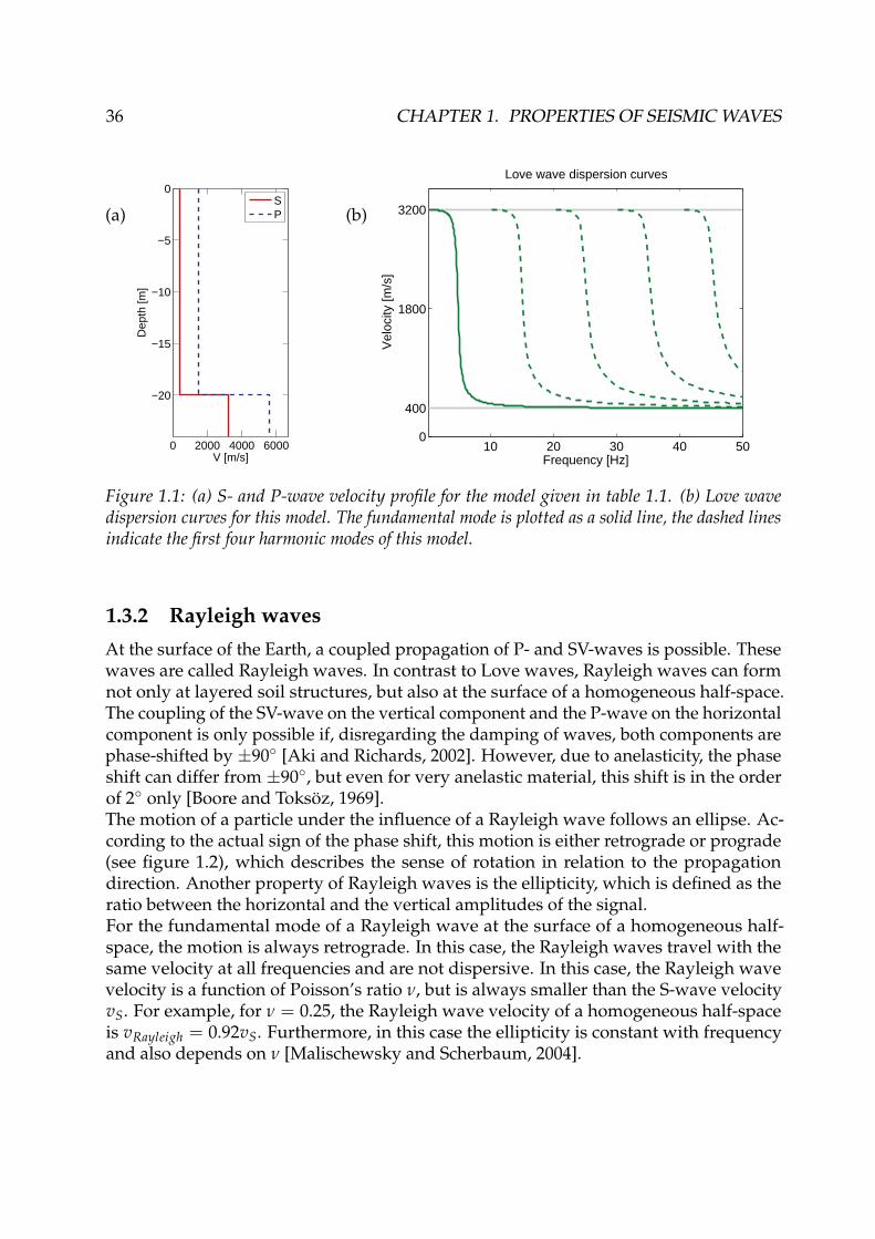
1.3.1 Love wavesThe existence of Love waves requires that the surface layer has a lower S-wave velocitythan the underlying structure. Therefore, the simplest soil structure for which Lovewaves can occur consists of a single layer overlying a homogeneous half-space withhigher S-wave velocity. In this case, SH-waves are reflected both at the surface and at theinterface between layers. The waves which are trapped in this way, are called Love waves.As Love waves consist of SH-waves, the motion of a surface particle under the influenceof a Love wave is parallel to the surface. Consequently, Love waves can only be recordedon the horizontal components of a seismic sensor. In contrast to body waves, Love wavestravel with different velocities at different frequencies. Furthermore, harmonic modesof motion are possible. A very simple soil structure model is given in table 1.1. The P-and S-wave velocity profiles for this model are shown in figure 1.1 (a). Figure 1.1 (b)shows the Love wave dispersion curves for this model for the fundamental and the firstfour higher modes. This figure illustrates that the fundamental mode is present over thewhole frequency range, while the harmonic modes occur at higher frequencies one afteranother. The Love waves’ phase velocity is always comprised between the minimumand maximum S-wave velocities of the soil structure.

Table 1.1: Parameters of a very simple soil structure model: Thickness range d, pressure wavevelocity VP, shear wave velocity VS and density ρ of the layers.

d[m] VP[m/s] VS[m/s] ρ[kg/m3]

0−20 1 500 400 2 00020−∞ 5 600 3 200 2 000

IAssuming an undamped wave propagation, the total energy of a seismic wave will remain constant asit travels away from the source. For surface waves, at a distance r from the origin, this energy is dispersedon a ring of circumference 2πr. For body waves, the energy is dispersed on the surface of a half-sphere2πr2. As the energy of a wave is proportional to its amplitude squared, the amplitudes of surface andbody waves decrease as 1√

r and 1r , respectively.

36 CHAPTER 1. PROPERTIES OF SEISMIC WAVES

(a)

0 2000 4000 6000

−20

−15

−10

−5

0

V [m/s]

Dep

th [m

]

SP (b)

10 20 30 40 500

400

1800

3200

Frequency [Hz]

Vel

ocity

[m/s

]

Love wave dispersion curves

Figure 1.1: (a) S- and P-wave velocity profile for the model given in table 1.1. (b) Love wavedispersion curves for this model. The fundamental mode is plotted as a solid line, the dashed linesindicate the first four harmonic modes of this model.

1.3.2 Rayleigh waves

At the surface of the Earth, a coupled propagation of P- and SV-waves is possible. Thesewaves are called Rayleigh waves. In contrast to Love waves, Rayleigh waves can formnot only at layered soil structures, but also at the surface of a homogeneous half-space.The coupling of the SV-wave on the vertical component and the P-wave on the horizontalcomponent is only possible if, disregarding the damping of waves, both components arephase-shifted by ±90◦ [Aki and Richards, 2002]. However, due to anelasticity, the phaseshift can differ from ±90◦, but even for very anelastic material, this shift is in the orderof 2◦ only [Boore and Toksöz, 1969].The motion of a particle under the influence of a Rayleigh wave follows an ellipse. Ac-cording to the actual sign of the phase shift, this motion is either retrograde or prograde(see figure 1.2), which describes the sense of rotation in relation to the propagationdirection. Another property of Rayleigh waves is the ellipticity, which is defined as theratio between the horizontal and the vertical amplitudes of the signal.For the fundamental mode of a Rayleigh wave at the surface of a homogeneous half-space, the motion is always retrograde. In this case, the Rayleigh waves travel with thesame velocity at all frequencies and are not dispersive. In this case, the Rayleigh wavevelocity is a function of Poisson’s ratio ν, but is always smaller than the S-wave velocityvS. For example, for ν = 0.25, the Rayleigh wave velocity of a homogeneous half-spaceis vRayleigh = 0.92vS. Furthermore, in this case the ellipticity is constant with frequencyand also depends on ν [Malischewsky and Scherbaum, 2004].

1.3. SURFACE WAVES 37

�v

retrograde particle motion

�v

prograde particle motion

Figure 1.2: Diagram of retro- and prograde Rayleigh wave motion.

(a)

10 20 30 40 500

400

1800

3200

Frequency [Hz]

Vel

ocity

[m/s

]

Rayleigh wave dispersion curves

(b)

10 20 30 40 500.001

0.01

0.1

1

10

100

1000

Frequency [Hz]

Vel

ocity

[m/s

]

Rayleigh wave ellipticity curves

Figure 1.3: (a) Rayleigh wave dispersion curve for the fundamental and the first four harmonicmodes for the model given in table 1.1. The fundamental mode is plotted as combination of a solidand a dotted line, where the solid line indicates retrograde particle motion and the dashed lineprograde motion. The dispersion curves for the higher modes are given by dash-dotted lines. (b)Ellipticity curves for the same modes. At the right flank of the fundamental mode, the particlemotion is prograde, whereas it is retrograde at the left flank and above the trough frequency. Theharmonic modes are indicated by colored dash-dotted lines.

For a layered structure, however, Rayleigh waves are dispersive, the ellipticity varies withfrequency and the wave motion can be prograde or retrograde, depending on frequency.The ellipticity as a function of frequency can show different behaviors, depending onthe soil model. In case of a layer overlying a half-space, the ellipticity curve exhibitsboth a singularity peak and a trough if the impedance contrast between the uppermostlayer and the half-space is strong (i.e. vS2 > vS2). In this case, the particle motion for thefundamental Rayleigh wave mode is prograde in the frequency range between the peakand the trough, i.e. for the right flank of the peak. For the other parts of the ellipticitycurve, the motion is retrograde. If the velocity profile does not exhibit a strong contrast,the ellipticity curve can still exhibit a peak, but neither a singular peak nor a trough. Then,the motion of the fundamental Rayleigh wave mode is retrograde for all frequencies.

38 CHAPTER 1. PROPERTIES OF SEISMIC WAVES

In figure 1.3 (a), the dispersion curves for the fundamental and the first four harmonicmodes of Rayleigh waves are shown for the model given in table 1.1. The fundamentalmode is present at all frequencies, whereas each harmonic mode is present above aspecific frequency only. At this frequency, the velocity of each mode equals the S-wavevelocity at the second layer. At high frequencies, the fundamental mode does not reachdeep enough to be influenced by the half-space. Therefore, its behavior is the same ason a half-space which has the properties of the surficial layer. Notably, for the modelcurves shown in figure 1.3 (a), the Rayleigh wave velocity is smaller than the respectiveS-wave velocity at frequencies above 15 Hz. In the opposite case, at very low frequencies,the Rayleigh wavelength is so large that the influence of the surficial layer becomesnegligible and the wave behaves as on the top of a half-space. The ellipticity curves ofthe model are shown in figure 1.3 (b). For the fundamental mode, the curve exhibits asingularity peak and a trough and becomes flat at higher frequencies. Between the peakand trough frequencies, the Rayleigh wave motion is prograde and retrograde at theother frequencies. The ellipticity curves for the other modes show a more complicatedbehavior with multiple peaks and troughs.

1.4 Conclusion

The seismic wave field is dominated by four types of waves: P-, S-, Love and Rayleighwaves. Among them, Love and Rayleigh waves appear to be very interesting for retriev-ing information on the soil structure due to their dispersion properties. The dispersion ofLove and Rayleigh waves can be depicted in a simple way. With increasing frequency, thewavelength decreasesII. Surface waves are confined to the surface and their amplitudesdecrease exponentially with depth. This decay depends on the wavelength. Conse-quently, a wave with a larger wavelength samples the soil structure to larger depths thana wave of smaller wavelength. Therefore, the low frequency part of the dispersion curvedepends on a thicker part of the soil structure than the high frequency part. In general,the velocities of seismic waves increase with depth and low frequency surface wavestravel faster than at higher frequencies.Another important property carrying information on the soil structure is the ellipticity ofRayleigh waves. In contrast to the measurement of Love and Rayleigh wave dispersioncurves, which can only be measured by using an array of seismic sensors, the ellipticitycan be measured using a single seismic station. Nevertheless, the retrograde or progradesense of rotation cannot be retrieved using a single seismic station because these nota-tions only make sense in combination with the direction of propagation which cannot bemeasured by a single sensor.

IIFrequency f and wavelength λ are linked via the wave velocity v (or the slowness s = 1v ) in a simple

way:v = λ · f .

Chapter 2

Single-sensor methods to estimate thepolarization of seismic waves

This chapter presents methods which can be used to characterize the polarization ofseismic waves using single sensors. First, some examples of established methods willbe shown, including rectilinearity and planarity filters as well as a method using theanalytic signal. Then, the widespread H/V technique is explained, before introducingDELFI and RayDec, two new methods which have been developed in the framework ofthis thesis work.

Ce chapitre présentera des méthodes pour caractériser la polarisation d’ondes sismiques enn’utilisant qu’un seul capteur. D’abord, quelques exemples de méthodes établies seront montrés,dont des filtres de réctilinéarité et de planarité et une méthode utilisant le signal analytique.Après, la technique très répandu du rapport H/V sera expliqué avant d’introduire DELFI etRayDec, deux méthodes nouvelles développées dans le cadre de ce travail de thèse.

39

40 CHAPTER 2. SINGLE-SENSOR METHODS

2.1 Introduction

This chapter is devoted to the estimation of polarization parameters of seismic wavesusing single seismic sensors. The estimation of polarization is an important problem as itallows the discrimination between different wave types, e.g. body and surface waves,Love and Rayleigh waves. The knowledge of the wave properties and the compositionof the wave field are important issues for various problems. These range from char-acterizing the wave source (i.e. estimating the azimuth and the incident angle) or thepropagation medium (wave velocities of the different wave types, damping parameters)to the estimation of site effects (Rayleigh wave ellipticity). Some of these characteristics,for example the wave velocity, can only be estimated using simultaneous recordingsof the wave field by multiple seismic sensors, but some others, like the Rayleigh waveellipticity, can be determined using single seismic sensors. Seismic array methods will betreated in chapters 3 and 4, the focus of the present chapter lies on single-sensor methods.

The motion of a Rayleigh wave is confined in the plane formed by the vertical and theradial component. The motion of a Love wave, however, is linear, i.e. confined to asingle horizontal direction. The basic idea of the methods which are presented in sections2.2.1[Flinn, 1965, Montalbetti and Kanasewich, 1970, Jurkevics, 1988] is to develop filterswhich estimate the rectilinearity (i.e. the confinement of the signal in its dominant polar-ization direction) and planarity (i.e. the confinement in a plane). Using these filters, timewindows with predominant rectilinear movement, i.e. P-, S- or Love waves, or planarmovement, i.e. Rayleigh waves, can be extracted from the signal recordings. All thesemethods are based on eigenvalue decompositions of real signal covariance matrices.The method presented in section 2.2.2 [Vidale, 1986], uses the analytic signal instead ofcovariance matrices, but the objective of the method is the same. The use of the analyticsignal allows in principle a more precise temporal signal characterization, as it is notnecessary to average over multiple time samples as in the other methods.

The other presented methods aim to estimate the Rayleigh wave ellipticity. The firstmethod, H/V [Nogoshi and Igarashi, 1971, Nakamura, 1989], presented in section 2.2.3,simply calculates the spectral ratio between the horizontal and the vertical components.This ratio is indeed linked to the resonance of the structure [Bonnefoy-Claudet et al., 2006]and corresponds to the Rayleigh wave ellipticity if the wave field consists exclusively ofRayleigh waves. However, in the presence of Love waves, the H/V curve misestimatesellipticity.

During this thesis work, two new methods have been developed which are speciallydesigned to estimate ellipticity. The first method, DELFI, is based on the direct fitting ofellipses to time windows of the signal. The second method, RayDec, suppresses otherwave types than Rayleigh waves by statistical means in order to estimate the ellipticityusing ambient seismic vibrations. Both methods are presented in detail in sections 2.3and 2.4, respectively.

2.2. OVERVIEW OF EXISTING METHODS 41

2.2 Overview of existing methods

2.2.1 Rectilinear and planar polarization filters

2.2.1.1 Rectilinear polarization filter

The filter presented in the following was originally developed by Flinn [1965]. The filterdetects the instantaneous linearity of a seismic signal and efficiently suppresses noisecontributions. It is primarily designed to enhance the recordings of transient signalsgenerated by earthquakes.In a first step, the signals are rotated in the azimuth direction, which separates radialand transverse contributionsI. For a time window of N data samples centered at t, thecovariance matrix is calculated. Let

X(t) =

R(t1) R(t2) · · · R(t) · · · R(tN)T(t1) T(t2) · · · T(t) · · · T(tN)Z(t1) Z(t2) · · · Z(t) · · · Z(tN)

(2.1)

be a 3× N data matrix describing the seismic records around the time t, where R, T andZ indicate the recordings of the radial, transverse and vertical components, respectively.Then the associated covariance matrix is given by

C(t) =1N

XT(t)X(t). (2.2)

The eigenvalues of C(t) are λ1, λ2 and λ3 (with λ1 > λ2 > λ3). Now, a function describingthe rectilinearity of the signal is defined by

G(λ1, λ2) = 1− λ2

λ1. (2.3)

If the signal has a principal polarization direction, λ1 will be large compared to λ2 andG(λ1, λ2) close to unity. In the opposite case, λ1 and λ2 will be comparable and G(λ1, λ2)small.This filter technique was improved by Montalbetti and Kanasewich [1970] by adding anarbitrary parameter n in equation (2.3), which transforms to

F(λ1, λ2) = 1−(

λ2

λ1

)n. (2.4)

The rectilinearity of the signal at time t is then given by

RL(t) = (F(λ1, λ2))J , (2.5)

where J is an additional arbitrary parameter. ~e1 =( eR

eTeZ

), the eigenvector associated to λ1,

indicates the direction of maximum polarization, i.e. the repartition of the wave energy

IThe azimuth is either given if the earthquake epicenter is known or has to be detected by an arraymethod.

42 CHAPTER 2. SINGLE-SENSOR METHODS

on the different components. In this way, time-dependent direction functions can bedefined by raising the different components of the eigenvector to an arbitrary power K,which yields

DR(t) = (eR)K , (2.6)

DT(t) = (eT)K , (2.7)

DZ(t) = (eZ)K . (2.8)

By changing the arbitrary constants n, J and K in equations (2.4) - (2.8) of the method, theresults can be tunedII. By averaging over some neighbouring values, the rectilinearityRL(t) and direction functions can be smoothed. The final signals are then obtained by

R f (t) = R(t) · RL(t) · DR(t), (2.9)

Tf (t) = T(t) · RL(t) · DT(t), (2.10)

Z f (t) = Z(t) · RL(t) · DZ(t). (2.11)

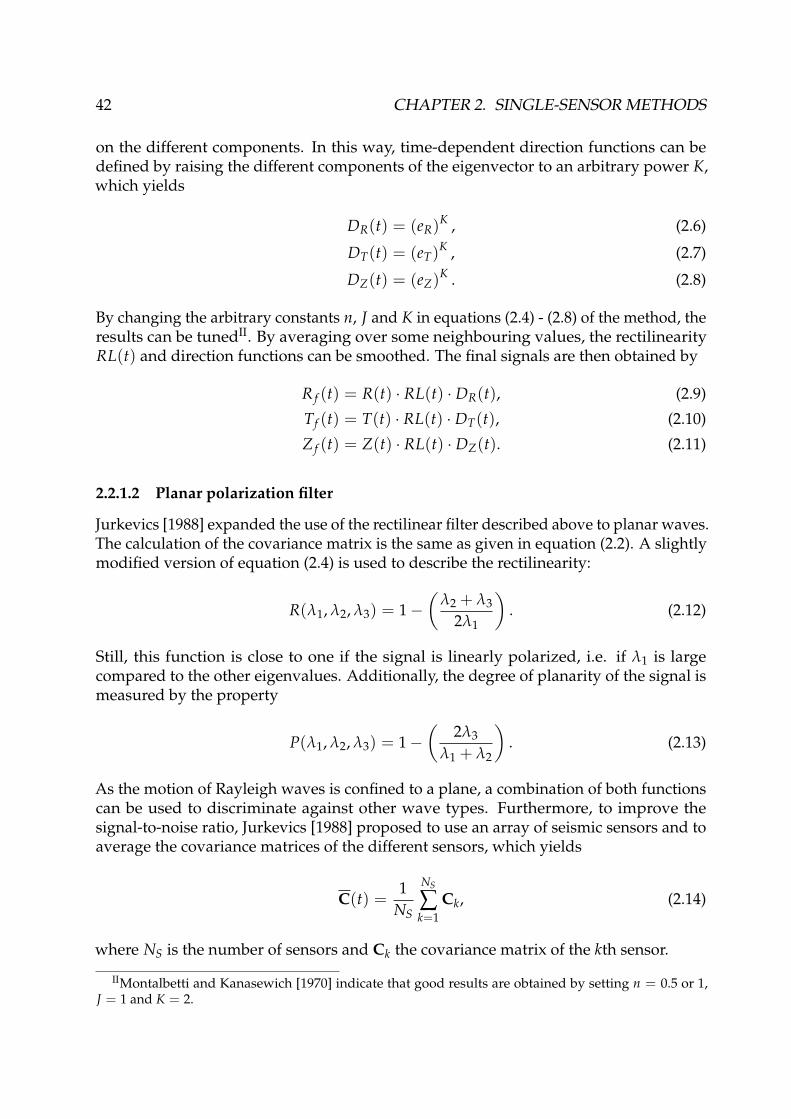
2.2.1.2 Planar polarization filter

Jurkevics [1988] expanded the use of the rectilinear filter described above to planar waves.The calculation of the covariance matrix is the same as given in equation (2.2). A slightlymodified version of equation (2.4) is used to describe the rectilinearity:

R(λ1, λ2, λ3) = 1−(

λ2 + λ3

2λ1

). (2.12)

Still, this function is close to one if the signal is linearly polarized, i.e. if λ1 is largecompared to the other eigenvalues. Additionally, the degree of planarity of the signal ismeasured by the property

P(λ1, λ2, λ3) = 1−(

2λ3

λ1 + λ2

). (2.13)

As the motion of Rayleigh waves is confined to a plane, a combination of both functionscan be used to discriminate against other wave types. Furthermore, to improve thesignal-to-noise ratio, Jurkevics [1988] proposed to use an array of seismic sensors and toaverage the covariance matrices of the different sensors, which yields

C(t) =1

NS

NS

∑k=1

Ck, (2.14)

where NS is the number of sensors and Ck the covariance matrix of the kth sensor.

IIMontalbetti and Kanasewich [1970] indicate that good results are obtained by setting n = 0.5 or 1,J = 1 and K = 2.

2.2. OVERVIEW OF EXISTING METHODS 43

2.2.2 Polarization analysis using the analytic signalThe following method has been proposed by Vidale [1986]. If the real-valued three-component measurements for a single seismic sensor are given by xk,r(t) (where k ∈{1,2,3} indicates the direction; 1 stands for eastern, 2 for northern and 3 for verticalcomponent), the analytic signal is built by

xk(t) = xk,r(t) + iH(xk,r(t)), (2.15)

where H represents the Hilbert transform, defined by H( f (x)) = 1π

∫ ∞−∞

f (x)y−x dx. In

this way, the real-valued signals become complex (without increasing the informationcontent). In fact, the analytic signal corresponds to a real signal where all negativefrequency contributions have disappeared without changing the signal’s energy, i.e. inthe Fourier transform the positive frequency contributions have doubled. By using theanalytic signal, it is possible to calculate an instantaneous covariance function

C(t) =

x1(t)x∗1(t) x1(t)x∗2(t) x1(t)x∗3(t)x2(t)x∗1(t) x2(t)x∗2(t) x2(t)x∗3(t)x3(t)x∗1(t) x3(t)x∗2(t) x3(t)x∗3(t)

. (2.16)

As the covariance matrix is by construction Hermitian, its eigenvalues λn (n ∈ {1, 2, 3},

λ1 > λ2 > λ3) are real, whereas the normed eigenvectors ~un =(

un,1un,2un,3

)are, in general,

complex. The eigenvector associated to the largest eigenvalue λ1 indicates the directionof maximum polarization. In fact, ~u1 represents a set of eigenvectors which are associatedto λ1. The product of ~u1 and eiα (with an arbitrary α) is still an eigenvector, becauseC~u1eiα = λ1eiα. From this set of eigenvectors, the vector whose real component ismaximum is chosen. This is done by searching the α maximizing the length X of the realcomponent of ~u1eiα given by

X =∣∣∣<(~u1eiα)

∣∣∣ . (2.17)

The elliptical polarization component is estimated by

PE =√

1− X2

X. (2.18)

Due to the normalization of ~u1, the length of the complex part of ~u1 is given by√

1− X2

and PE represents the ratio between imaginary and real part of the eigenvector. For linearpolarization, PE = 0, and for circular polarization, PE = 1. By using the components of~u1, the azimuth ϑ and angle of incidence δ of the wave can be estimated by

ϑ = arctan(<(u1,2)<(u1,1)

), (2.19)

δ = arctan

(<(u1,3)√

(<(u1,1))2 + (<(u1,2))2

), (2.20)

44 CHAPTER 2. SINGLE-SENSOR METHODS

where u1,k indicates the component of ~u1 in direction k. Further polarization parameterscan be defined in a way similar to the rectilinearity and planarity filters of Jurkevics[1988]. The strength of polarization is defined in a way slightly different from equation(2.12) by

PS = 1−(

λ2 + λ3

λ1

)(2.21)

and the degree of planarity is estimated by

PP = 1−(

λ3

λ2

). (2.22)

If the signal is polarized with a single dominant component, PS is close to 1. If the signalin both other components is comparable to the dominant one, PS is low. In the same way,PP is close to 1 if the intermediate component is much larger than the smallest one andclose to 0 if both components are comparable.The advantage of using the analytic signal is that the analysis can be performed for eachtime sample independently, i.e. without having to average over a time window in theseismogram as would be necessary when using real-valued signals, but it is necessaryto use the time-series of the signal to calculate the Hilbert transform. Nevertheless, themethod can only work if a single seismic signal is present. If two waves arrive at thesame time, calculating the analytical signal gives wrong results.

2.2.3 H/V

The horizontal-to-vertical (H/V) method was introduced by the publication (in Japaneselanguage) of Nogoshi and Igarashi [1971] and popularized among the English-speakingscience community by Nakamura [1989]. Since then, it is a widespread technique whichhelps to characterize the soil by simple means. The method consists in the calculationof the ratio between the horizontal and vertical Fourier spectra of the seismic noiserecordings of a single three-component seismic sensor. If the Fourier transforms of therecordings of the three components are Xeast( f ), Xnorth( f ) and Xvert( f ), respectively,then the H/V ratio is calculated byIII

H/V =

√|Xeast( f )|2 + |Xnorth( f )|2

|Xvert( f )| . (2.23)

Although the theory behind the H/V ratio is not yet completely understood, empiricalevidence shows that a peak in the H/V curve is correlated with the resonance frequencyof the structure [Bonnefoy-Claudet et al., 2006, Haghshenas et al., 2008]. Furthermore, fora single Rayleigh wave crossing the structure, the H/V ratio corresponds to the definitionof the ellipticity curve. However, in the general case Love waves are also present [Köhleret al., 2006, Endrun, 2010] and the H/V ratio will not provide the ellipticity.

IIISometimes, this ratio is defined with an additional√

2 in the denominator.

2.3. DELFI 45

2.3 DELFI

The following method has been developed during this work. DELFI (Direct ELlipseFItting for Rayleigh wave ellipticity estimation) is a method which estimates the ellipticityof Rayleigh waves by directly fitting an ellipse to the filtered data [Hobiger et al., 2009b].There are two processing steps, the first one determines the vertical plane where thesignal is confined and projects the signal in this plane, the second fits an ellipse to theobtained two-dimensional signal. Figure 2.1 gives an overview of the principles of themethod. The algorithm is explained in the following.

2.3.1 Plane detection

Consider the three-dimensional signal recorded by a single seismic sensor. This signalcan be represented as a time series S(t) = [E(t) N(t) Z(t)], where E(t), N(t) and Z(t)are the signals of the eastern, northern and vertical component, respectively. In thisway the signal S(t) takes values in R3. In a first step, the signal S(t) is filtered around acentral frequency f with a filter bandwidth d f which yields the filtered signal Sf(t) =[E f (t) N f (t) Z f (t)

].

Then, for each frequency of interest, the following processing is performed independently.First, the filtered signal is cut into blocks of time length T = nP/ f , which correspondsto signals of nP periods at the given frequency. If we denote the sample rate of theoriginal signal by dt, each cut block of signal includes N = T/dt data points. The three-component signal of one of these blocks Sb = [Eb Nb Zb] forms a matrix of dimensionN × 3. The starting and ending times of a block are given by tb,s and tb,e, respectively.As the polarization of Rayleigh waves is confined to a plane formed by a horizontal anda vertical axis, the first step is to identify the vertical plane where the signal is confinedthe most. This is done by using the signal of both horizontal components. The planecan be defined by its normal vector~a = (aE, aN)T. For each data point ~pi = (Ei, Ni), thedistance to the plane is given by di = ~pi ·~a. We fit the plane in a least-squares sense byminimizing the functional

D =N

∑i=1

d2i , (2.24)

which can be written in matrix form as

D = (p ·~a)T(p ·~a)=~aT · pT · p ·~a=~aT · S ·~a, (2.25)

where p = [Eb Nb] is the matrix of all data points and S = pT · p the position covariancematrix. The normalized eigenvectors ~ui (with associated eigenvalues λi, for i ∈ {1, 2},with λ1 < λ2) of S form a basis of the two-dimensional space.

46 CHAPTER 2. SINGLE-SENSOR METHODS

(a)

−50

−25

0

25

50

−25

0

25

−25

0

25

EastNorth

Ver

tical

(b)

−1

0

1

−2

−1

0

1

2−0.5

0

0.5

EastNorth

Ver

tical

(c)

−1

0

1

−2

−1

0

1

2−0.5

0

0.5

EastNorth

Ver

tical

(d)

−1

0

1

−2

−1

0

1

2−0.5

0

0.5

EastNorth

Ver

tical

(e)

−2 −1 0 1 2−1.5

−1

−0.5

0

0.5

1

1.5

Horizontal

Ver

tical

(f)

−2 −1 0 1 2−1.5

−1

−0.5

0

0.5

1

1.5

h

v

Horizontal

Ver

tical

Figure 2.1: Graphic outline of the DELFI method: (a) A single three-component seismic sensorrecords a time series of data points in 3D space. (b) The signal is filtered around f , the frequencyof interest. (c) The filtered signal is cut into blocks of equal length (typically one period). (d) Eachof these blocks is extracted and the plane, where the signal is confined, is searched for. (e) Thesignal block is projected into this plane. (f) An ellipse is fitted. Repeated processing of steps (d)-(f)for every signal block cut in (c) yields the ellipticity estimation at frequency f .

2.3. DELFI 47

Therefore,~a can be expressed as a linear combination of ~u1 and ~u2 by

~a =2

∑i=1

ki~ui. (2.26)

Thus, exploiting the properties S~ui = λi~ui and ~uTj ~ui = δij, the functional can be written

as

D =2

∑i=1

2

∑j=1

kik j~uTi S~uj

=2

∑i=1

2

∑j=1

kik j~uTi ~ujλj

=2

∑i=1

2

∑j=1

kik jδijλj

= k21λ1 + k2

2λ2 (2.27)

As the vector~a is normalized, k21 + k2

2 = 1. As λ1 < λ2, D is minimized by k1 = 1 andk2 = 0. It follows that~a = ~u1. As~a is the normal vector of the plane, the other eigenvector~u2 and the vertical unit vector span the plane. The horizontal components Eb and Nb cannow be projected onto the vector ~u2 to form the horizontal signal

Hb = [Eb Nb] · ~u2. (2.28)

In this way, the original three-dimensional signal is transformed into the two-dimensionalsignal

S′b = [Hb Zb]. (2.29)

2.3.2 Ellipse fitting

The next step consists in fitting an ellipse to the data matrix S′b. Fitzgibbon et al. [1999]proposed an algorithm which fits an ellipse to any two-dimensional cloud of datapoints. In general, six parameters are necessary to define a two-dimensional ellipse: twocoordinates defining the center point and two two-dimensional vectors defining the semi-major and semi-minor axes, respectivelyIV. Of course, the ellipse can be parameterizedin a different way without changing the number of necessary parameters. For thecase where we search for Rayleigh waves, the number of parameters can be reducedconsiderably. Firstly, we know that the center point of the ellipse must lie on the originof the sensor’s coordinate systemV.

IVIn the three-dimensional case, nine parameters are necessary: each of the three vectors is defined bythree parameters. In the three-dimensional case, the plane of the ellipse can be easily found by using athree-dimensional covariance matrix. By projecting the signal on this plane, the problem reduces to thetwo-dimensional case.

VThe presence of different signals, especially of frequency content different from the analyzed Rayleighwave, could shift the ellipse including the center point. This effect is inhibited by the narrow-band filteringin the first step of the processing.

48 CHAPTER 2. SINGLE-SENSOR METHODS

In addition, both axes of the ellipse of the Rayleigh wave motion lie in the horizontaland vertical direction if the soil is perfectly elastic. Boore and Toksöz [1969] showed thatanelasticity leads to a shift of the phase angle between the vertical and the horizontalmotion. However, they showed that even for very anelastic material (Qα = 10, Qβ = 4,β = 0.55α) this shift does not exceed 2◦. As such a shift is hardly ever measurable, weimpose that both axes lie in horizontal and vertical direction, respectively. In this way,the Rayleigh wave motion can be parameterized by only two parameters, namely thehorizontal and the vertical axes. Both are necessary to calculate ellipticity.The following function describes an ellipse with a horizontal and a vertical axis:

ax2 + by2 − 1 = 0, (2.30)

where a and b are parameters related to the horizontal and vertical axes, respectively. Ifwe denote the lengths of the horizontal and the vertical axes by h and v, respectively, thefollowing relations hold:

a =1h2 , b =

1v2 . (2.31)

The distance of an arbitrary point (x, y) from the ellipse is given by

F(x, y) = ax2 + by2 − 1. (2.32)

To a set of data points (xi, yi) with i ∈ {1, 2, . . . , N}, an ellipse can be fitted by minimizingthe functional

D =N

∑i=1

F(xi,yi)2. (2.33)

This leads to the following set of equations:

∂D∂a

= aN

∑i=1

x4i + b

N

∑i=1

x2i y2

i −N

∑i=1

x2i = 0, (2.34)

∂D∂b

= aN

∑i=1

x2i y2

i + bN

∑i=1

y4i −

N

∑i=1

y2i = 0. (2.35)

This can be written in matrix form as

S · ~A = ~C, (2.36)

with

S =(

∑ x4i ∑ x2

i y2i

∑ x2i y2

i ∑ y4i

), (2.37)

~A =(

ab

), (2.38)

~C =(

∑ x2i

∑ y2i

), (2.39)

2.3. DELFI 49

where the summations stretch over all indices 1 ≤ i ≤ N. This equation can be easilysolved byVI

~A = S−1 · ~C. (2.40)

The properties a and b can be transformed into the horizontal and vertical axes by usingequation (2.31).The presented ellipse-fitting algorithm is applied to every signal block Sb, which yieldsthe horizontal and vertical axes hb and vb, as well as the value of the functional D whichserves as weighting factor Db. This processing is performed for all signal blocks and theellipticity at frequency f is finally calculated by

εDELFI( f ) = ∑b hb/Db

∑b vb/Db. (2.41)

2.3.3 Free parameters

Table 2.1: Values for the horizontal and vertical axes as well as the resulting ellipticity for theellipse fits of figure 2.2.

Used data points Horizontal axis Vertical axis Ellipticity

original ellipse 2.000 1.000 2.00all points 2.072 0.973 2.13left half 2.058 0.951 2.16

right half 2.085 0.993 2.10quarter 1 2.008 1.051 1.91quarter 2 2.012 0.933 2.16quarter 3 2.086 0.975 2.14quarter 4 2.220 0.923 2.41

In the algorithm, there are only two free parameters: d f , the bandwidth of the filterand nP, the number of periods in each signal block. The filter bandwidth should beadjusted in such a way to exclude contributions of other frequencies to a maximum. Thenumber of periods in the signal block should not exceed 1, as the amplitude of seismicwaves can evolve with time. Therefore, it is improbable that two subsequent signalblocks have the same amplitude, even if their respective ellipticities are identical. Theellipse-fitting algorithm does not set a lower boundary of how much signal has to beprocessed. However, the sample rate dt of the signal sets a lower limit for nP, as anellipse estimation based on two or three data points does not make much sense. In thesame time, if only a part of the ellipse is covered by data points, the ellipse estimation

VIIn the general case, the position covariance matrix S is invertible. However, if the data points lie on adegenerated ellipse, i.e. on a line, S will be singular and cannot be inverted. Then, S can be transformedinto an invertible form by adding small numbers on the diagonal entries.

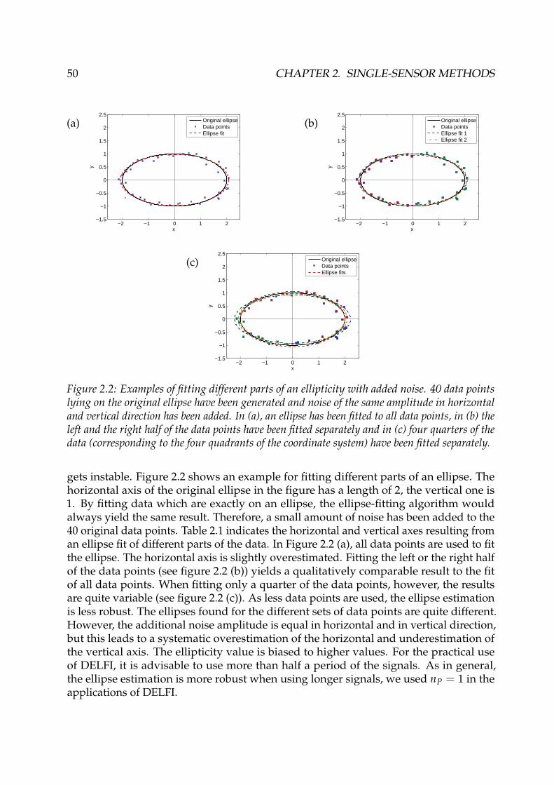
50 CHAPTER 2. SINGLE-SENSOR METHODS

(a)

−2 −1 0 1 2−1.5

−1

−0.5

0

0.5

1

1.5

2

2.5

x

y

Original ellipseData pointsEllipse fit

(b)

−2 −1 0 1 2−1.5

−1

−0.5

0

0.5

1

1.5

2

2.5

x

y

Original ellipseData pointsEllipse fit 1Ellipse fit 2

(c)

−2 −1 0 1 2−1.5

−1

−0.5

0

0.5

1

1.5

2

2.5

x

y

Original ellipseData pointsEllipse fits

Figure 2.2: Examples of fitting different parts of an ellipticity with added noise. 40 data pointslying on the original ellipse have been generated and noise of the same amplitude in horizontaland vertical direction has been added. In (a), an ellipse has been fitted to all data points, in (b) theleft and the right half of the data points have been fitted separately and in (c) four quarters of thedata (corresponding to the four quadrants of the coordinate system) have been fitted separately.

gets instable. Figure 2.2 shows an example for fitting different parts of an ellipse. Thehorizontal axis of the original ellipse in the figure has a length of 2, the vertical one is1. By fitting data which are exactly on an ellipse, the ellipse-fitting algorithm wouldalways yield the same result. Therefore, a small amount of noise has been added to the40 original data points. Table 2.1 indicates the horizontal and vertical axes resulting froman ellipse fit of different parts of the data. In Figure 2.2 (a), all data points are used to fitthe ellipse. The horizontal axis is slightly overestimated. Fitting the left or the right halfof the data points (see figure 2.2 (b)) yields a qualitatively comparable result to the fitof all data points. When fitting only a quarter of the data points, however, the resultsare quite variable (see figure 2.2 (c)). As less data points are used, the ellipse estimationis less robust. The ellipses found for the different sets of data points are quite different.However, the additional noise amplitude is equal in horizontal and in vertical direction,but this leads to a systematic overestimation of the horizontal and underestimation ofthe vertical axis. The ellipticity value is biased to higher values. For the practical useof DELFI, it is advisable to use more than half a period of the signals. As in general,the ellipse estimation is more robust when using longer signals, we used nP = 1 in theapplications of DELFI.

2.4. RAYDEC 51

2.4 RayDec

The name RayDec stands for "Rayleigh wave ellipticity estimation using the randomdecrement technique". Figure 2.3 gives an overview of the principles of the method.The technique was published in Geophysical Review Letters, the following article ("SingleStation Determination of Rayleigh Wave Ellipticity by Using the Random DecrementTechnique (RayDec)" by Hobiger, Bard, Cornou, and Le Bihan, 2009a) describes themethod in detail.

2.4.1 Abstract

Rayleigh wave ellipticity as a function of frequency is closely linked to undergroundstructure, i.e. shear wave velocity profile and sediment thickness. The possibilityto calculate these underground properties by inverting ellipticity curves has recentlybeen shown. We propose a new technique enabling the Rayleigh wave ellipticity to berecovered over a wide frequency range by using ambient noise recordings. Based on therandom decrement technique commonly used to characterize dynamic parameters ofbuildings, this method eliminates all wave types except Rayleigh waves. We apply themethod to noise synthetics simulated for different underground structures and show itsapplicability to real seismic noise data.

2.4.2 Introduction

In order to properly evaluate local site amplification it is important to have a goodknowledge of the local soil properties, i.e. shear-wave velocities and sediment thickness.These soil properties can be obtained by inverting dispersion curves. One way is to usethe dispersion curves of surface waves, as derived from active or passive seismic arraymeasurements. However, it usually provides reliable information at frequencies higherthan the resonance frequency and the inverted velocity profiles do not carry informationon the deeper structures. Additional information around the resonance frequency can beadded by using H/V spectra. Recent studies have shown the possibility to evaluate theS-wave velocity profile by inversion of H/V spectra [Fäh et al., 2003, Arai and Tokimatsu,2004] or joint inversion of H/V spectra and dispersion curves [Arai and Tokimatsu, 2005,Picozzi et al., 2005]. The classical H/V technique [Nakamura, 1989] calculates the ratiobetween the horizontal and the vertical spectrum of ambient vibrations recorded on a

single three-component seismic sensor by H/V( f ) =√|E( f )|2+|N( f )|2√

2 |Z( f )| where E( f ), N( f )

and Z( f ) are the spectra of the east-west, north-south and vertical displacements ofthe sensor. Both Rayleigh and Love waves contribute to the H/V spectrum [Bonnefoy-Claudet et al., 2008] and the presence of both surface wave types has to be accountedfor in inversion algorithms. Therefore, the proportion between Rayleigh and Lovewaves in the noise wave field has to be inferred or assumed prior to the inversion[Scherbaum et al., 2003, Arai and Tokimatsu, 2004, Köhler et al., 2006]. Extraction ofRayleigh wave ellipticity and its subsequent inversion [Boore and Toksöz, 1969, Fäh et al.,2001, Malischewsky and Scherbaum, 2004] would avoid making such assumptions.

52 CHAPTER 2. SINGLE-SENSOR METHODS

(a)

0 2 4 6 8 10

Z

0 2 4 6 8 10

E

0 2 4 6 8 10

N

Time [s]

(b)

0 2 4 6 8 10

Z

0 2 4 6 8 10

E

0 2 4 6 8 10

N

Time [s]

(c)

0 2 4 6 8 10

Z

0 2 4 6 8 10

E

0 2 4 6 8 10

N

Time [s]

(d)

0 1 2 3 4 56

54

32

1

N

E

Z

Time [s]Signal block

(e)

0 1 2 3 4 56

54

32

1

H

Z

Time [s]Signal block

(f)

0 1 2 3 4 5

Z

0 1 2 3 4 5

H

Time [s]

Figure 2.3: Graphic outline of the RayDec method: (a) A single three-component seismic sensorrecords a time series of data. (b) On the vertical component of the filtered signal, all zero crossingsfrom negative to positive are searched for. (c) For every identified zero crossing, signals of length∆ are extracted on all three components, delaying the horizontal by 1

4 f , which corresponds to thevertical 90◦ phase shift to the vertical component. (d) These signal blocks are stacked. (e) Bothhorizontal signals are projected in the direction which maximizes the correlation to the verticalsignal. (f) All these signals are summed, which yields a single vertical and horizontal signal. Theellipticity at frequency f is then estimated by comparing the respective energies of these summedsignals.

2.4. RAYDEC 53

We propose a new method (RayDec) to estimate the Rayleigh wave ellipticity spectrumby using the random decrement technique [Asmussen, 1997]. A usual application of therandom decrement technique is the measurement of resonance frequencies and dampingparameters of buildings [Dunand, 2005, Michel et al., 2008]. We propose to apply therandom decrement technique to three-component seismometer records of seismic noise.By using the vertical component as a master trigger and stacking a large number ofhorizontal and vertical signals, Rayleigh waves will be emphasized with respect to Loveand body waves. Therefore, the obtained ellipticity curve will be closer to the true curvethan the H/V curve.In this paper, we will present the method, apply it to synthetic seismic noise and finallyshow its applicability to real seismic noise records with one example.

2.4.3 Methodology

Assume that a three-component sensor record consists of three time-series of seismicnoise (e(t) in east-west direction, n(t) in north-south direction and v(t) in vertical di-rection). Each of these time-series has a time length T and consists of N data points. Inorder to extract the ellipticity of Rayleigh waves we suggest the following method, basedon the random decrement technique [Asmussen, 1997]. The principles of the methodare to emphasize Rayleigh waves with respect to other wave types by summing a largenumber of specially tuned signal windows, calculate the energy on the vertical andhorizontal summed signals and henceforward estimate Rayleigh wave ellipticity. Thefirst step consists of filtering the signals by using a narrow-band Chebyshev filter of order4 and bandwidth d f centered on frequency f . We use the Chebyshev filter because of itssharpness. Filtering was performed on a linear frequency scale. The resulting signals arecalled e f (t), n f (t) and v f (t).

Then we search for all times τi where the signal on the vertical component changes itssign from negative to positive (v f (τi) ≤ 0, v f (τi + dt) > 0). Every time this condition issatisfied, we store signals of length ∆ on all three components, leading to buffered signalsv f ,b,i(t), e f ,b,i(t) and n f ,b,i(t) defined in terms of the original signals as (for 0 ≤ t ≤ ∆):

v f ,b,i(t) = v f (τi + t),

e f ,b,i(t) = e f (τi −1

4 f+ t), (2.42)

n f ,b,i(t) = n f (τi −1

4 f+ t).

The shift of 14 f on the eastern and northern components accounts for the 90◦ phase shift

between the vertical and horizontal components of Rayleigh waves. Then we build ahorizontal signal h f ,b,i(t) by projecting the east-west and north-south components ontoan axis forming an azimuth angle ϑi with the northern direction by

h f ,b,i(t) = sin(ϑi) · e f ,b,i(t) + cos(ϑi) · n f ,b,i(t). (2.43)

54 CHAPTER 2. SINGLE-SENSOR METHODS

The angle ϑi is chosen in such a way that it maximizes the correlation between the verticalsignal v f ,b,i(t) and the horizontal signal h f ,b,i(t) given by:

C f ,b,i(ϑi) =∫ ∆

0v f ,b,i(t) · h f ,b,i(t)dt

C f ,b,i(ϑi) = sin(ϑi)∫ ∆

0v f ,b,i(t) · e f ,b,i(t)dt + cos(ϑi)

∫ ∆

0v f ,b,i(t) · n f ,b,i(t)dt. (2.44)

The correlation is maximized by

ϑi = tan−1

( ∫ ∆0 v f ,b,i(t) · e f ,b,i(t)dt∫ ∆0 v f ,b,i(t) · n f ,b,i(t)dt

). (2.45)

There are two possible ϑi ∈ [0◦, 360◦[ satisfying equation (2.45), with ϑi,2 = ϑi,1 + 180◦,one of them leading to a negative, the other to a positive correlation. The ϑi leading to apositive correlation is chosen. The method does not distinguish between prograde andretrograde particle motion as prograde Rayleigh waves are treated as retrograde wavesarriving from the opposite azimuth.

Although the chosen angle ϑi maximizes the correlation between v f ,b,i(t) and h f ,b,i(t),the correlation can be low. Thus, we make use of the correlation factor defined as

c f ,b,i =

∫ ∆0 v f ,b,i(t) · h f ,b,i(t)dt√∫ ∆

0 v2f ,b,i(t)dt ·

∫ ∆0 h2

f ,b,i(t)dt. (2.46)

In the case of perfect correlation between v f ,b,i(t) and h f ,b,i(t) this factor equals 1. On theother side, it will vanish when the vertical and horizontal signals are not correlated at all.The signals v f ,b,i(t) and h f ,b,i(t) are weigthed by c2

f ,b,i and summed for all times τi toobtain two buffered signal windows of length ∆:

v f ,S(t) = ∑i

c2f ,b,i · v f ,b,i(t) (2.47)

h f ,S(t) = ∑i

c2f ,b,i · h f ,b,i(t). (2.48)

Finally, the ellipticity ε is calculated as the square root of the ratio of the energies in thebuffered signal windows h f ,S(t) and v f ,S(t):

ε =

√√√√∫ ∆0 (h f ,S(t))2dt∫ ∆0 (v f ,S(t))2dt

. (2.49)

By repeated filtering of the signal over the entire frequency range and applying the pre-sented method the ellipticity of Rayleigh waves as a function of frequency is determined.

2.4. RAYDEC 55

Figure 2.4: S- and P-wave velocity profiles for the models N101, N102, N103 and N104 [Cornouet al., 2009]. The original figure has been modified to improve the readability.

The free parameters of the method are the width of the frequency filter d f and the lengthof the buffered signal ∆.

It could be supposed that Love and body waves influence the results. In an assumedisotropic medium, Love waves are not present on the vertical component and theirhorizontal movements are thus uncorrelated with the vertical signal. Although incidentalcorrelations of Love and Rayleigh waves arriving at the same time cannot be excluded,such effects will rapidly lose importance because of stacking and can thus be neglected.Arriving P- and S-waves can be present on the vertical and horizontal components, butas their movements are not phase delayed, they will also disappear due to averagingover a sufficiently large number of windows.

2.4.4 Application to synthetic noiseIn order to test the method, we used a set of synthetic noise simulated for the modelsN101, N102, N103 and N104 of the ESG 2006 benchmark [Cornou et al., 2009]. Thecompressional (P) and shear wave (S) velocity profiles of these models are displayed infigure 2.4.The noise synthetics were obtained in the following way: Noise sources were approxi-mated by forces of random orientation and amplitude located 0.5 m below the surface[Moczo and Kristek, 2002]. The forces are randomly distributed in time and space. Thetime function of each source is a delta-like signal with a flat Fourier frequency-amplitudespectrum between 0.1 and 20 Hz. In this frequency range, the associated wave fieldhas been computed by using the wavenumber-based technique for horizontally layeredstructures proposed by Hisada [1994, 1995]. All types of surface and body waves areincluded in the simulations.

56 CHAPTER 2. SINGLE-SENSOR METHODS

2.4.4.1 Influence of the parameters of the method

As mentioned above, there are two free parameters that can be adjusted to improve theperformance of the method: d f , the width of the frequency filter, and ∆, the length ofthe buffered signal. To investigate the optimal parameters, we used 30 minutes of noisesimulated for the model N102. The noise sources are located in the far field as well as inthe local field.Figure 2.5 (a) shows the calculated ellipticity for different bandwidths d f of the fre-quency filter compared to the theoretical ellipticity of the model. The used bandwidthsare proportional to the central frequencies. Too weak filtering (d f = 0.5 f ) as well as toostrong filtering (d f = 0.1 f ) do not give satisfying results. An intermediate setting of0.2 f reproduces the real curve the best. Therefore, we fixed the bandwidth to 0.2 f in thefollowing.Figure 2.5 (b) shows the resulting ellipticity for different lengths ∆ of the buffered signalwindows in comparison to the theoretical curve. We fix ∆ as a function of frequency,so that the signals consist of the same number of periods at all frequencies. As can beseen in the figure, at least ten cycles are necessary for a good coverage of the signalwhereas further increasing of the window length does not improve the results. Therefore,∆ = 10/ f is used in the following.

2.4.4.2 Minimum required signal length and temporal stability of the results

The required signal length is illustrated in figure 2.5 (c). The same signals as in sub-subsection 2.4.4.1 were used and the first 1800, 600, 300 and 120 seconds of signal wereanalyzed. The results of the analysis for signals of 1800, 600 and 300 seconds onlyslightly differ. However, the curve obtained for 120 seconds of signal is less smooththan the other curves. At low frequencies, the signal statistics deteriorate due to thesmaller number of buffered windows. It can be deduced that - for sites with resonancefrequencies around 1 Hz - a signal length of five minutes can be sufficient to measure anaccurate ellipticity curve, as long as enough Rayleigh waves are present in the signal. Forsmaller underground resonance frequencies, the measurement has to be longer. Indeed,longer measurements improve the statistical features and the reliability of the results atall frequencies.The temporal stability of the obtained ellipticity curves is shown in figure 2.5 (d). Fivedifferent synthetic signals of ten minutes each were simulated and the ellipticity curveswere calculated for each window. The overall behavior of the curves is identical. Only thefourth ten-minute-window shows some instabilities between 0.1 and 0.2 Hz emphasizingthe need for longer signal lengths at low frequencies. For the other frequencies, the fiveellipticity curves are very close. This illustrates the temporal stability of the results.

2.4. RAYDEC 57

1 10

1

10

Elli

ptic

ity

Frequency [Hz]

(a)modeldf=0.5fdf=0.3fdf=0.2fdf=0.1f

1 10

1

10

Elli

ptic

ity

Frequency [Hz]

(b)modelΔ=1/fΔ=5/fΔ=10/fΔ=20/f

1 10

1

10

Frequency [Hz]

Elli

ptic

ity

(c)modelT=120sT=300sT=600sT=1800s

1 10

1

10

Frequency [Hz]

Elli

ptic

ity

(d)

model

1st 10 minutes

2nd 10 minutes

3rd 10 minutes

4th 10 minutes

5th 10 minutes

Figure 2.5: Sensitivity of the results with respect to the parameters of the method demonstratedon simulated seimic noise for the N102 model. The real ellipticity curve of the model is includedfor comparison. Curves (a) and (b) were calculated for 30 minutes of simulated seismic noise. (a)Effect of the filter bandwidth d f on the resulting ellipticity curve (∆ = 10/ f ) for d f = 0.5 f ,d f = 0.3 f , d f = 0.2 f and d f = 0.1 f . (b) Effect of the length ∆ of the buffered signal(d f = 0.2 f ) for ∆ = 1/ f , ∆ = 5/ f , ∆ = 10/ f and ∆ = 20/ f . (c) Effect of the length ofthe signals (time length T, d f = 0.2 f , ∆ = 10/ f ) for T = 1800s, T = 600s, T = 300s andT = 120s. (d) Analysis of five different signals of ten minutes each (d f = 0.2 f , ∆ = 10/ f ).The original figure has been modified to improve the readability.

2.4.4.3 Results for the models N101, N103 and N104

RayDec has been applied to synthetic noise simulated for different models. The resultsof these simulations are shown in figure 2.6. For model N101 (figure 2.6 (a)), the curve isclose to the real curve over the whole frequency range, although the peak ellipticity isoverestimated. For this model layout, reflected body waves can deteriorate the results.Therefore, more signal would be needed to obtain a more robust ellipticity curve. Formodel N103 (figure 2.6 (b)), there is a good agreement between the simulated and thetheoretical curves around the resonance frequency and at higher frequencies, with someminor deviations between 0.3 and 2 Hz.

58 CHAPTER 2. SINGLE-SENSOR METHODS

1 10

1

2

4

Elli

ptic

ity

Frequency [Hz]

(a)modelH/VRayDec

0.1 1 10

0.5

1

2

5

10

Elli

ptic

ity

Frequency [Hz]

(b)modelH/VRayDec

1 10

0.5

1

2

5

10

20

Elli

ptic

ity

Frequency [Hz]

(c)model fundamental modemodel 1st harmonic modeH/VRayDec

1 10

0.5

1

2

5

10E

llipt

icity

Frequency [Hz]

(d)borehole modelH/VRayDec

Figure 2.6: Ellipticity curves obtained for ten minutes of synthetic noise simulated for threedifferent underground models (N101(a), N103 (b) and N104 (c)) and for one hour of real noisefrom Colfiorito basin (d). The used parameters are d f = 0.2 f and ∆ = 10/ f . In the fourgraphs, the results are compared to the real ellipticity curves of the fundamental mode and thefirst harmonic mode (only in (c)) and to the results obtained by the H/V technique. Curve (d)also contains the error ranges of the H/V and RayDec curves. The original figure has beenmodified to improve the readability.

Below 0.15 Hz, the curve differs considerably from the theoretical curve. Model N104(figure 2.6 (c)) exhibits some unfavorable behavior, as the fundamental mode and thefirst harmonic mode of Rayleigh wave motion overlap above 1.4 Hz. RayDec cannotdistinguish between two modes. Therefore, its results are a mixture of the two modesin this frequency range. For lower frequencies, RayDec reproduces well the theoreticalcurve around the first peak of the fundamental mode. The H/V curve follows the sametrend, but the absolute values of the RayDec curve better reproduce the right flank of thefundamental peak.It can be stated that, in general, the results of RayDec are much closer to the theoreticalcurves than the results obtained with the H/V method. However, RayDec regularly failsin reproducing very small ellipticity values. At these points, the horizontal componentsof the Rayleigh wave vanish.

2.4. RAYDEC 59

Therefore, it is problematic to find horizontal signals correlated to the vertical signal. Thesame reasoning is valid for the peak frequency ellipticity in the case of a theoreticallyvanishing vertical component. This explains why the peak ellipticity cannot be satisfac-torily estimated. On the other hand, small ellipticities can also be hidden by the presenceof higher Rayleigh wave modes. In cases where higher Rayleigh wave modes are closeto the fundamental modes, RayDec only indicates an apparent ellipticity which cannotbe simply related with the true ellipticity of each mode.

2.4.5 Application to real noise dataTo test the RayDec method on real data, we applied it to one hour of seismic noiserecorded in the center of Colfiorito basin in central Italy. Colfiorito basin is a well-known site which has been extensively investigated by different geophysical methods[Di Giulio et al., 2006]. The theoretical ellipticity curve is calculated on the basis of S-and P-wave velocity profiles obtained by a borehole measurement (see figure 2.4). Theparameters used were d f = 0.2 f and ∆ = 10/ f . The hour of signal was cut into sixten-minute signals which were analyzed separately. The resulting curves were thenaveraged. When comparing with the theoretical ellipticity curve, one should keep inmind that a borehole measurement is made at a selected point, whereas a seismic noiserecord is influenced by the whole surrounding underground structure. The RayDeccurve is in better agreement with the theoretical curve than the H/V curve, especially onthe slopes of the fundamental resonance frequency peak (figure 2.6 (d)). However, boththe H/V and RayDec curve’s peak frequencies are shifted with respect to the boreholemodel’s peak frequency.

2.4.6 Conclusion

RayDec is a fast and simple method to determine the ellipticity of Rayleigh waves.As it suppresses Love and body waves efficiently, its results are closer to theory thanH/V results. The necessary signal length depends on the resonance frequency of theunderground structure, but some minutes of signal can be sufficient to get satisfyingresults, as long as enough Rayleigh waves are present in the wave field, although longersignal lengths are preferable. However, as it is a one-sensor technique, RayDec givestwo possible azimuths and cannot distinguish between prograde and retrograde particlemotion. By coupling RayDec with array measurements the correct azimuth and the senseof particle motion could be retrieved. Besides that, it could be envisaged to estimate theproportion of Rayleigh waves in the wave field by comparing RayDec results includingonly Rayleigh waves with H/V measurements including all wave types. The futurework consists of trying to improve the inversion of S-wave velocity profiles by usingRayDec’s ellipticity estimations. This is a non-trivial endeavor which will be addressedin a future paper.

60 CHAPTER 2. SINGLE-SENSOR METHODS

2.5 Conclusion

One of the main fields of interest of this thesis is the measurement and use of the ellip-ticity of Rayleigh waves. The rectilinearity and planarity filters indicate which wavetype is predominant at a given time and can be used to discriminate against undesiredwave types and enhance the desired signal part. However, these methods do not allowthe direct retrieval of ellipticity and will not be considered in the following chapters.Nevertheless, they could be used as a preprocessing step for real data applications or forstudies on specific seismic phases (P, S, surface waves).

The new methods DELFI and RayDec, as well as H/V, will be tested on synthetic seismicsignals in chapter 5. In chapter 6, the potentials and limitations of the inversion ofellipticity curves will be investigated. These inversions will subsequently be applied toreal data measurements collected during the NERIES project for 14 European sites inchapter 7. The ellipticity curves used for these inversions will be measured by RayDec.A concise overview of DELFI and RayDec was presented at the European Signal Pro-cessing Conference (EUSIPCO) 2009 in Glasgow (UK). The associated paper ("Rayleighwave ellipticity estimation from ambient seismic noise using single and multiple vector-sensor techniques" by Hobiger, Le Bihan, Cornou, and Bard, 2009b) which includes acomparison with the MUSIQUE technique (see section 4.6) can be found in appendix A.

Chapter 3

Characterization of seismic waves usingarrays of sensors

This chapter is dedicated to methods characterizing seismic waves using arrays of seis-mic sensors. The conventional beamforming method, frequency-wavenumber analysisand MUSIC techniques will be presented before focusing on the SPAC method. For thismethod, we will investigate the influence of the number of seismic sensors used on theresolution of the method, proofing mathematically that an increasing (odd) number ofring stations is directly linked to a resolution increase. Finally, 2s-SPAC, a method usingonly two seismic stations, is presented and tested on real data measurements.

Ce chapitre est dédié aux méthodes caractérisant les ondes sismiques à l’aide de réseaux decapteurs sismiques. La formation de voies conventionnelle, l’analyse fréquence-nombre d’ondeet la méthode MUSIC seront présentées avant de présenter la méthode SPAC plus en détail.L’influence du nombre de capteurs utilisés sur la résolution de la méthode sera examinée,montrant mathématiquement qu’un nombre croissant (impair) de capteurs sur l’anneau induitdirectement une augmentation de résolution. Finalement, 2s-SPAC, une méthode n’utilisantque deux capteurs sismiques, sera présentée et testée sur des données sismiques réelles.

61

62 CHAPTER 3. SEISMIC ARRAY METHODS

3.1 Introduction

Arrays of seismic sensors are an important tool to investigate the soil properties. In fact,a single seismic sensor cannot determine the complete wave vector, i.e. velocity andazimuth, of incident seismic waves. Nevertheless, in chapter 2, it has been shown thatthe polarization parameters of the wave can be estimated using a single sensor. Thecomplete wave vector can be determined using arrays of seismic sensors. Therefore,two-dimensional arrays of seismic sensors are used in seismology. An example for thelayout of such an array is given in figure 3.1 (a). The basic principle of every arraymethod is that an incident wavefront arrives at the different stations at different timesI.From the arrival time delays of the signals recorded at the respective stations, the wavevelocity v (or its inverse, the slowness s) and the azimuth can be retrieved. It is clear thata one-dimensional seismic array (i.e. a line of sensors) is not able to retrieve azimuthor velocity, because it can only determine the component of the wave vector which liesin the array directionII. Azimuth and velocity can only be found when both horizontalcomponents of the wave vector are resolved.

Furthermore, a two-dimensional seismic array can only find the "apparent" velocity ofthe wave. If a plane wave is arriving under an angle of incidence γ (see figure 3.1 (b))from the vertical axis, the apparent velocity is given by va = v/ sin γ, where v is theactual wave velocity (the apparent slowness is given by sa = s · sin γ, where s is the actualslowness). Notably, for an angle of incidence of 0◦, the apparent velocity is infinite andthe wave arrives at the same time at all stations. In order to retrieve the actual velocity,azimuth and angle of incidence of a wave, a three-dimensional array would need to beused. This requires sensors in boreholes with depths comparable to the deploymentsize at the surface. Thus, apart from being quite expensive, such measurements aretime-consuming.

However, only body waves as S- and P-waves can arrive under an angle of incidencedifferent from 90◦. Surface waves, like Love and Rayleigh waves, are travelling horizon-tally. Therefore, surface waves can be analyzed using two-dimensional seismic arrays.In the following, some well-known investigation methods using seismic arrays willbe presented in detail. Conventional beam-forming (section 3.2) is the simplest andmost intuitive of these methods. The azimuth and velocity of an incident wave is deter-mined by delaying the signals of the different sensors according to different azimuth andvelocity values and identifying those values maximizing the total energy. The frequency-wavenumber method [Lacoss et al., 1969, Capon, 1969] presented in section 3.3 can beseen as the transformation of the conventional beam-forming method from the time do-main in the frequency domain. The MUSIC method [Schmidt, 1986] shown in section 3.4is another algorithm which allows the estimation of the number of signals and separates

IIn general, a seismic wave radiating from a point source has a curved wave front. If the distancebetween a seismic array and the source is large compared to the array size, however, the wave front isalmost plane.

IIIf either the azimuth or the wave velocity are known, the other parameter can be determined by aone-dimensional array. However, the azimuth estimation for a known velocity is still ambiguous.

3.1. INTRODUCTION 63

signal from noise space. The advancement of this code by including quaternions andbiquaternions will be the topic of chapter 4. All these methods allow the determinationof wave velocity and azimuth of incoming waves.

A different approach to measure the wave velocity using ambient seismic vibrationsis the spatial autocorrelation (SPAC) technique [Aki, 1957], which will be presented inmore detail in section 3.5. This technique measures the wave velocity by averaging thecorrelations between stations located on a ring and the central station. After introducingthe methodology, we will investigate the theoretical resolution of the technique for arraysof different sizes and show a mathematical proof for the resolution increase caused by anincrease of the number of stations on the ring. The M-SPAC approach [Bettig et al., 2001]facilitates SPAC measurements as it suppresses the need of equidistant station spacingof the original method. Finally, the 2s-SPAC method [Morikawa et al., 2004] will bepresented, which substitutes the spatial averaging over many station pairs by a temporalaveraging of a single moving station pair. We will apply this method to measurementsperformed in Patras, Greece, and show its usefulness for real data measurements insection 3.5.7.

(a)

1

23

4

5

6

7 89

10

ϑ

k

wave front

Eastern coordinate

Nor

ther

n co

ordi

nate

(b)

0

wave front

γ

Ver

tical

coo

rdin

ate

Horizontal coordinate

(c)

0 5 10 15

10

9

8

7

6

5

4

3

2

1

Time [s]

Sen

sor

num

ber

(d)

0 5 10 15Time [s]

undelayed sumdelayed sum

Figure 3.1: (a) Diagram of a seismic array with incident plane wave arriving under an azimuthangle ϑ. (b) If the wave is arriving with an angle of incidence different from 90◦, the array willdetect an apparent velocity va = v/ sin γ. (c) Theoretical signals of the different sensors for theincident wave in (a). (d) Undelayed sum und delayed sum of the signals from (c).

64 CHAPTER 3. SEISMIC ARRAY METHODS

3.2 Delay-and-sum beamforming

The simplest and probably the most intuitive way of treating recordings of seismic arraysis delay-and-sum beamforming [Christensen and Hald, 2004]. The basic idea is to bringthe recordings of the different seismic stations into phase by compensating the timedelays induced by the respective travel time differences.An incident wave will arrive at the different stations of the array at different times, ascan be seen in figure 3.1 (c), where the signals of the different stations due to the incidentwave in figure 3.1 (a) are shown. Let the slowness vector of the incident wave be givenby

~s( f ) = s( f ) ·

− sin ϑ sin γ− cos ϑ sin γ

cos γ

, (3.1)

where s( f ) = |~s( f )| is the absolute value of the slowness vector, ϑ the azimuth and γ theangle of incidence of the wave. Defining the matrix R ∈ RN×3 as the position matrix ofthe N seismic stations of the array, the delay vector ~∆(~s( f )) = R~s( f ) indicates the delayscorresponding to the different seismic stations with respect to the origin (not necessarilya sensor position).The recorded signals bi(t) (i ∈ {1, 2, . . . , N}) of the seismic sensors are filtered aroundthe frequency f , which results in band-pass filtered signals b f ,i(t). They include a signalpart s f ,i(t) and a noise part n f ,i(t):

b f ,i(t) = s f ,i(t) + n f ,i(t). (3.2)

In order to identify the azimuth and slowness of an incident wave, a grid search can beperformed. For each pair of slowness s and azimuth ϑ, the corresponding delay vector iscalculated, the signals of the different sensors are delayed accordingly and summed toproduce the final signal b~s(t)III:

b f ,~s(t) =1N

N

∑i=1

w f ,i b f ,i(t + ∆i(~s( f ))),

=1N

N

∑i=1

wi s f ,i(t + ∆i(~s( f ))) +1N

N

∑i=1

wi n f ,i(t + ∆i(~s( f ))). (3.3)

Here, the wi are optional weighting factors. The correct slowness vector can now beidentified by calculating the energy content for the signals b f ,~s(t) by

E f (~s) =L

∑l=1

b2f ,~s(tl)dt, (3.4)

where l ∈ 1, . . . , L parameterizes the time samples. The ~s( f ) corresponding to themaximum of E f (~s) characterizes the incident wave. The associated b f ,~s(t) can be seen asan enhanced version of the incident signalIV.

IIIIf the delays of the different sensors can be identified precisely,~s can be calculated directly by R−1~∆.IVAs the signal parts in equation (3.3) superpose constructively whereas the noise parts do not, the signal

can be improved by using a large number of seismic sensors. The signal-to-noise ratio increases as√

N.

3.3. FREQUENCY-WAVENUMBER ANALYSIS 65

In figure 3.1 (d), the result of a direct summation of the signals at the different sensorsis compared to the result of the delayed sum of signals. The direct summation is notrepresenting the actual signal.For simple cases, where a single wave is incident, the delay-and-sum beamforming canyield satisfactory results. Nonetheless, if multiple waves interfere, the resolution of thissimple method may not be sufficient. Therefore, more sophisticated methods exist.

3.3 Frequency-wavenumber analysis

The frequency-wavenumber analysis [Lacoss et al., 1969] can be seen as beamformingin the frequency domain. If we consider a single incident plane wave whose slownessvector~s0( f ) is given by equation (3.1) arriving at an array of N seismic sensors (withrespective sensor positions~ri, i ∈ {1, 2, . . . N}). The first sensor’s position is the originof the coordinate system. Then, the respective (single-component) recordings of thedifferent stations can be written as

xi(t) =∞∫−∞

C( f )ei2π f (t−~s0( f ) ~ri)d f , (3.5)

where C( f ) is the frequency-dependent complex amplitude of the wave. It is possible todefine the array signal vector ~x(t) as

~x(t) =

x1(t)x2(t)

...xN(t)

=∞∫−∞

C( f )ei2π f (t−R ~s0( f ))d f , (3.6)

where R is the matrix of sensor locations (of size N × 3). The Fourier transform of thesignal vector yields

~X( f ) =1√2π

∞∫−∞

∞∫−∞

C( f ′)ei2π f ′(t−R ~s0( f ′))e−i2π f td f ′dt

=1√2π

∞∫−∞

C( f ′)e−i2π f ′R ~s0( f ′)∞∫−∞

ei2π( f ′− f )tdtd f ′

=1√2π

∞∫−∞

C( f ′)e−i2π f ′R ~s0( f ′)δ( f ′ − f )d f ′

=1√2π

C( f )e−i2π f R ~s0( f )

= S0( f )e−iR ~k0( f ), (3.7)

where S0( f ) = C( f )√2π

is the Fourier transform of the signal recorded at the station located

at the origin and~k0( f ) = 2π f~s0( f ) the wave vector.

66 CHAPTER 3. SEISMIC ARRAY METHODS

A steering vector can be defined by~a(~k) = 1√N

e−iR~k. Multiplying ~X( f ) by~a†(~k0) brings

all the components of ~X( f ) in phase and sums them. The energy of ~X( f )~a†(~k) is calcu-lated by

E f (~k) =∣∣∣~X†( f )~a(~k)

∣∣∣2=∣∣∣∣S0( f )ei(R ~k0( f ))T 1√

Ne−iR~k

∣∣∣∣2=

∣∣∣∣∣S0( f )1N

N

∑i=1

e−i~ri (~k−~k0( f ))

∣∣∣∣∣2

= |S0( f )|2∣∣∣∣∣ 1N

N

∑i=1

e−i~ri (~k−~k0( f ))

∣∣∣∣∣2

≤ |S0( f )|2 = E f (~k0). (3.8)

The correct wave vector~k0 can therefore be found by performing a grid search overall possible values of~k and identifying the maximum of E f (~k). The theoretical arrayresponse is given by

A(~k, f ) =

∣∣∣∣∣ 1N

N

∑i=1

e−i~ri ~k

∣∣∣∣∣2

, (3.9)

which corresponds to E f (~k)/ |S0( f )|2 for an incident wave whose wave vector is the zerovector, corresponding to infinite velocity (or a wave arriving under an angle of incidenceof 0◦).

3.3.1 Resolution limits of seismic arrays

A seismic array can only resolve seismic waves in a region of the frequency-slownessplane which is defined by the array layout. For example, an equidistant linear sensorantenna cannot resolve waves whose wavelengths are inferior to twice the minimumsensor distance dmin because of aliasing, which would correspond to a maximum wavenumber of kmax = 2π

2dmin. A rough estimation of the lower resolution limit can be given by

kmin = 2πdmax

, where dmax is the maximum inter-sensor distance in the array. However, fortwo-dimensional array layouts, the resolution limits are different for different azimuths.Using the array response function defined in equation (3.9), the resolution limits of thearray can be investigated for each azimuth. The question of array responses of two-dimensional arrays has been largely discussed in the literature, for example by Woodsand Lintz [1973], Asten and Henstridge [1984], Tokimatsu [1997], Gaffet et al. [1998] andWathelet et al. [2008].

3.4. MUSIC 67

3.4 MUSIC

The MUSIC method was originally developed by Schmidt [1986]. The name MUSICstands for "MUltiple SIgnal Classification". This algorithm allows the estimation of thenumber of signals and their associated directions of arrival for data recorded by an arrayof sensors. The basic idea behind the MUSIC algorithm is to separate the noise and signalsubspaces and subsequently estimate the signal parameters. The method is explained inthe following.An array of N monocomponent seismic sensors records a time series of seismic data. Kdifferent uncorrelated seismic waves impinge. Each wave is characterized by its wave

vector~ki = −2π f si( f )(

sin ϑicos ϑi

0

), where si( f ) is the slowness and ϑi the backazimuth of

the wave. Therefore, the signal ~X( f ) recorded at the different seismic stations can bewritten as a linear combination of the signals of the different sources plus noise. In partic-ular, this noise is not seismic noise, which would still carry information, but instrumentalor other noise. Thus, it is assumed that the noise contributions at the different sensorsare uncorrelated. An additional assumption is that the noise is uncorrelated to the truesignal. This yields the following expression for the signal:

X1( f )X2( f )

...XN( f )

=(~a(~k1), ~a(~k2), . . . , ~a(~kK)

)·

F1( f )F2( f )

...FK( f )

+

W1( f )W2( f )

...WN( f )

, (3.10)

or in matrix form

~X( f ) = A( f ) · ~F( f ) + ~W( f ). (3.11)

The signals are represented in the frequency-phase domain, corresponding to a Fouriertransform of the signals in time-space domain. The complex vector ~F ∈ CK×1 indicatesthe amplitude and phase (in reference to a given point) of the source signals. The vectors~a(~k) in matrix A ∈ CN×K describe the phase differences induced by the propagationbetween each source (defined by its wave vector~k ∈ R3×1) and each sensor. If R ∈ RN×3

is the matrix of sensor positions,

~a(~k) =1√N

exp(−iR ·~k). (3.12)

The vector ~W ∈ CN×1 characterizes the noise at each sensor. In this way, the signal~X ∈ CN×1 is a linear combination of source signals and noise terms. In the following, thefrequency arguments will be omitted, but it should not be forgotten that we work at agiven frequency.It is now possible to build a N × N covariance matrix S by

S = E(~X · ~X†

)= A · E(~F~F†)A† + E(~W ~W†), (3.13)

68 CHAPTER 3. SEISMIC ARRAY METHODS

where E(x) indicates the expectation value and the non-correlation of ~F and ~W is used.The correlation matrix simplifies to

S = APA† + λW0, (3.14)

where P = E(~F~F†) and W0 is the noise covariance matrix. We assume that the elementsof the noise vector W are distributed according to a normal distribution with zero meanand variance σ2, which yields λW0 = σ2I. Therefore,

S = APA† + σ2I. (3.15)

In general, the number of seismic sensors N is larger than the number of incident wavesK. Therefore, APA† is singular with a rank of K. The eigenvalue σ2 of S will occur(N − K) times. S has N eigenvectors ~ui (1 ≤ i ≤ N) with associated eigenvalues λi. Wecan write

S~ui = APA†~ui + σ2I~ui (3.16)

λi~ui = APA†~ui + σ2~ui (3.17)

APA†~ui = (λi − σ2)~ui. (3.18)

As the eigenvalue σ2 of S occurs (N − K) times, the corresponding eigenvectors ~ui (with1 ≤ i ≤ N − K) are orthogonal to APA† and to the space spanned by the column vectorsof A.In this way, these (N − K) eigenvectors span a noise subspace. The other K eigenvectorsspan the signal subspace. In a real data application, the number of sources is, in general,not known. Then, the number of signals can be estimated by considering the eigenvalues:the largest eigenvalues belong to the signal subspace and the remaining eigenvalues tothe noise subspace.We build the noise subspace G ∈ CN×N−K by

G = (~u1, ~u2, . . . , ~uN−K) . (3.19)

For a given~a(~k), the squared distance d2 to the signal subspace is calculated by

d2 = ‖G† ~a(~k)‖2

=(

G† ~a(~k))†

G† ~a(~k)

=~a†(~k) GG† ~a(~k), (3.20)

as the vectors spanning the noise subspace are orthogonal to the signal subspace. The~a(~k) which maximizes the MUSIC functional

P(~k) =1d2 =

1

~a†(~k) GG† ~a(~k)(3.21)

is in a certain way the most orthogonal to the noise subspace and therefore the mostconfined in the signal subspace. In this way the properties of the incident waves, i.e.azimuth and slowness, can be retrieved by a two-dimensional grid search.

3.5. SPATIAL AUTOCORRELATION TECHNIQUE (SPAC) 69

3.5 Spatial autocorrelation technique (SPAC)

The spatial autocorrelation technique (SPAC) has been developed by Aki [1957]V. As weuse this method extensively for the analysis of real seismic noise data, its methodologywill be presented in more detail. In contrast to the original derivation of Aki [1957], it isnot necessary to assume that different waves are uncorrelated, as will be shown in thefollowing.

3.5.1 Vertical componentFirst, we consider the vertical motion only. The motion of a seismic wave at a givenfrequency f can be written as a superposition of a number of seismic waves with differentwave vectors~kn by

u(~r, f , t) = ∑n

An( f ) cos(2π f t−~kn( f )~r + ϕn), (3.22)

where ϕn is the phase of the wave and~r the position of an arbitrary sensor. k( f ) =∣∣∣~kn( f )

∣∣∣is the absolute value of the wave vector. Wave vector and velocity at frequency f arelinked by k( f ) = 2π f /v( f ) = 2π f s( f ). The correlation between two sensors located at~r1 and~r2 can then be written as

φ(~r1,~r2, f ) =1T

T∫0

u(~r1, f , t) u(~r2, f , t)dt

φ(~r1,~r2, f ) =1T ∑

n∑m

An ( f )Am( f )

·T∫

0

cos(2π f t−~kn( f )~r1 + ϕn) cos(2π f t−~km( f )~r2 + ϕm)dt, (3.23)

where T has to be a multiple of 1/ f VI. The original derivation of Aki [1957] assumedthat different wave components are uncorrelated, i.e. ¯An Am = 0 for n 6= m, where thebar represents the averaging operation. In fact, this property is not necessary to derivethe SPAC equations as will be shown in the following.

VThe name is misleading, because indeed cross correlations between different sensors are calculated.

VIAlternatively, T has to be so large that 1T

T∫0

cos(2π f t)dt→ 0.

70 CHAPTER 3. SEISMIC ARRAY METHODS

By substituting a = 2π f t, b =~kn( f )~r1 − ϕn and c =~km( f )~r2 − ϕm, the integral can becalculated as

2π∫0

cos(a− b) cos(a− c)da =2π∫0

(cos a cos b + sin a sin b)(cos a cos c + sin a sin c)da

=2π∫0

cos2 a cos b cos c da +2π∫0

sin2 a sin b sin c da

+2π∫0

sin a cos a(sin b cos c + cos b sin c) da

=π(cos b cos c + sin b sin c)=π cos(b− c). (3.24)

By resubstituting a, b and c, equation (3.23) simplifies to

φ(~r1,~r2, f ) =12 ∑

n∑m

An( f ) Am( f ) cos(~kn( f )~r1 −~km( f )~r2 − ϕn + ϕm). (3.25)

Without restricting the universal validity of this formula, we can set the first sensoron the origin of the coordinate system and put a ring of seismic sensors at a radiusr around the first sensor. Then, the inner product of ~km( f ) and ~r2 can be written as~km( f )~r2 = −k( f )r cos(ϑm − γ), where ϑm is the azimuth of the mth incoming wave andγ the angle under which the sensor at~r2 is seen from the origin. The mean correlationbetween the central sensor and all sensors on the ring can then be written as

φ(r, f ) =1

2π

2π∫0

φ(0,~r2 = r · (sin γ, cos γ)T, f )dγ

=1

4π ∑n

∑m

An( f )Am( f )2π∫0

cos(k( f )r cos(ϑm − γ)− ϕn + ϕm)dγ

=1

4π ∑n

∑m

An( f )Am( f )2π∫0

cos(k( f )r cos γ) cos(ϕn − ϕm)dγ

+1

4π ∑n

∑m

An( f )Am( f )2π∫0

sin(k( f )r cos γ) sin(ϕn − ϕm)dγ.

=1

4π ∑n

∑m

An( f )Am( f )2π∫0

cos(k( f )r cos γ) cos(ϕn − ϕm)dγ. (3.26)

3.5. SPAC 71

By using2π∫0

cos(x cos γ)dγ = 2π J0(x), where J0(x) indicates the Bessel function of the

first kind of order 0VII, this equation can be simplified to

φ(r, f ) =12 ∑

n∑m

An( f )Am( f ) cos(ϕn − ϕm) · J0(k( f )r). (3.27)

The graph of J0(x) is plotted in figure 3.2. The autocorrelation of the central station isgiven by setting~r2 =~r1 (i.e. r = 0):

φ(0, f ) =12 ∑

n∑m

An( f )Am( f ) cos(ϕn − ϕm). (3.28)

Finally, dividing equation (3.27) by equation (3.28) yields

ρvertical(r, f ) =φ(r, f )φ(0, f )

= J0 (2π f r s( f )) . (3.29)

The meaning of this equation can be described as follows: If one disposes of a singleseismic sensor surrounded by a large number of sensors, then the correlation functionsbetween the central station and each ring sensor have to be calculated. Averaging allthese correlation functions and normalizing the result by the autocorrelation of the cen-tral station yields a curve which can be identified as J0 (2π f r s( f )). In this way, a directlink between the frequency and the slowness of the wave, i.e. its dispersion curve, isgiven.In the derivation of this function, it was integrated over γ, i.e. in such way that thepairs of correlated seismic sensors cover all possible azimuths. Replacing the integrationover γ by an integration over ϑ in the formula would not change the result. This wouldcorrespond to a single pair of seismic sensors and incoming waves covering all azimuths.This means that if the wave field was perfectly isotropic, i.e. if waves arrived fromall directions with identical energies, a single pair of seismic sensors would suffice tomeasure the correct Bessel function.

VIIThe Bessel functions of the first kind Jn(x) are solutions of the equation x2 d2ydx2 + x dy

dx + (x2 − n2)y = 0:

J0(x) =∞

∑k=0

(−1)k( x2 )2k

k!2, J1(x) =

∞

∑k=0

(−1)k( x2 )2k+1

(k + 1)! k!, J2(x) =

∞

∑k=0

(−1)k( x2 )2k+2

(k + 2)! k!.

72 CHAPTER 3. SEISMIC ARRAY METHODS

3.5.2 Horizontal components

The derivation described above is only valid for the vertical component. For bothhorizontal components of the seismic sensors, the reasoning is slightly different becausehorizontal waves can be polarized either in the transverse or in the radial direction.In general, on both horizontal components of a seismic sensor both polarizations arerecorded simultaneously.Considering two seismic sensors, the radial component is oriented in the directionconnecting both sensors. The transverse component is oriented in the perpendiculardirection.Let us assume in a first step that the horizontal wave field is composed exclusively ofwaves with radial polarization which arrive under respective azimuth angles ϑn. If thesecond seismic sensor is seen under an angle γ from position of the first sensor, i.e. theangle γ is defining the radial component of their respective recordings. Then the radialcomponent recording of any of both seismic sensors is given by

ur(~r, γ, f , t) = ∑n

An( f ) cos(2π f t−~kn( f )~r + ϕn) cos(ϑn − γ), (3.30)

whereas its transverse recording is given by

ut(~r, γ, f , t) = ∑n

An( f ) cos(2π f t−~kn( f )~r + ϕn) sin(ϑn − γ). (3.31)

The calculation of the correlation between the two sensors is analog to equations (3.23) -(3.25) with additional sinus or cosinus terms and will therefore not be shown in detail.The equation analog to equation (3.26) for the radial component is then given by

φr(r, f ) =1

4π ∑n

∑m

An( f )Am( f )

·2π∫0

cos(k( f )r cos(ϑm − γ)− ϕn + ϕm) cos(ϑn − γ) cos(ϑm − γ) dγ

=1

4π ∑n

∑m

An( f )Am( f )

·2π∫0

cos(k( f )r cos γ− ϕn + ϕm) cos(γ + ϑm − ϑn) cos γ dγ (3.32)

and for the transverse component by

φt(r, f ) =1

4π ∑n

∑m

An( f ) Am( f )

·2π∫0

cos(k( f )r cos γ− ϕn + ϕm) sin(γ + ϑm − ϑn) sin γ dγ. (3.33)

3.5. SPAC 73

The integral in equation (3.32) can be calculated by

2π∫0

cos(k( f )r cos γ− ϕn + ϕm) cos(γ + ϑm − ϑn) cos γ dγ

= cos(ϕn − ϕm) cos(ϑm − ϑn)2π∫0

cos(k( f )r cos γ) cos2 γ dγ

+ sin(ϕn − ϕm) cos(ϑm − ϑn)2π∫0

sin(k( f )r cos γ) cos2 γ dγ

− cos(ϕn − ϕm) sin(ϑm − ϑn)2π∫0

cos(k( f )r cos γ) sin γ cos γ dγ

− sin(ϕn − ϕm) sin(ϑm − ϑn)2π∫0

sin(k( f )r cos γ) sin γ cos γ dγ.

In this equation,2π∫0

cos(k( f )r cos γ) cos2 γ dγ = π(J0(k( f )r)− J2(k( f )r)) and all other

integrals vanish. The graph of J2(x) is shown in figure 3.2. Now, the correlation for theradial component can be expressed by

φr(r, f ) =14 ∑

n∑m

An( f )Am( f ) cos(ϕn − ϕm) cos(ϑm − ϑn)(J0(k( f )r)− J2(k( f )r)).

(3.34)

For the transverse component, the calculation is completely analog and yieldsVIII

φt(r, f ) =14 ∑

n∑m

An( f )Am( f ) cos(ϕn − ϕm) cos(ϑm − ϑn)(J0(k( f )r) + J2(k( f )r)).

(3.35)

The radial and transverse autocorrelations for the central station are calculated by

φr(0, f ) =14 ∑

n∑m

An( f )Am( f ) cos(ϕn − ϕm) cos(ϑm − ϑn), (3.36)

φt(0, f ) =14 ∑

n∑m

An( f )Am( f ) cos(ϕn − ϕm) cos(ϑm − ϑn). (3.37)

VIIIUsing2π∫0

cos(k( f )r cos γ) sin2 γ dγ = π(J0(k( f )r) + J2(k( f )r)).

74 CHAPTER 3. SEISMIC ARRAY METHODS

This finally generates the normalized correlation functions ρr(r, f ) and ρt(r, f ) for radiallypolarized waves:

ρradial,r(r, f ) =φr(r, f )φr(0, f )

= J0 (2π f r s( f ))− J2 (2π f r s( f )) , (3.38)

ρradial,t(r, f ) =φt(r, f )φt(0, f )

= J0 (2π f r s( f )) + J2 (2π f r s( f )) . (3.39)

The reasoning for transversely polarized waves is completely analogue. In this case,however, the radial component’s recording is given by

ur(~r, γ, f , t) = ∑n

An( f ) cos(2π f t−~kn( f )~r + ϕn) sin(ϑn − γ), (3.40)

whereas its transverse recording is given by

ut(~r, γ, f , t) = ∑n

An( f ) cos(2π f t−~kn( f )~r + ϕn) cos(ϑn − γ). (3.41)

This means that the equation for the radial component in this case is the same as forthe transverse component in the case of radially polarized waves (equation (3.31)) andthat the transverse component’s record is described as the radial component in equation(3.30). Therefore, we can directly give the resulting autocorrelation functions ρr(r, f ) andρt(r, f ) for transverse wave polarization:

ρtransverse,r(r, f ) = J0 (2π f r s( f )) + J2 (2π f r s( f )) , (3.42)ρtransverse,t(r, f ) = J0 (2π f r s( f ))− J2 (2π f r s( f )) . (3.43)

3.5.3 Rayleigh and Love waves

The SPAC method is particularly adapted to analyze seismic noise recordings. In a realcase, the noise wave field will always be composed of both Rayleigh and Love waves(neglecting body waves). The Rayleigh wave dispersion curve can then be retrieved byusing the vertical autocorrelation function ρvertical(r, f ) defined in equation (3.29). Thehorizontal components are not easy to analyze, however, as Love and Rayleigh wavesboth contribute with an unknown percentage. Rayleigh waves are radially polarized andLove waves are transverse waves. Therefore, we can identify

ρRayleigh,v(r, f ) = ρvertical(r, f ) (3.44)

ρRayleigh,r(r, f ) = ρradial,r(r, f ) (3.45)

ρRayleigh,t(r, f ) = ρradial,t(r, f ) (3.46)

ρLove,r(r, f ) = ρtransverse,r(r, f ) (3.47)ρLove,t(r, f ) = ρtransverse,t(r, f ). (3.48)

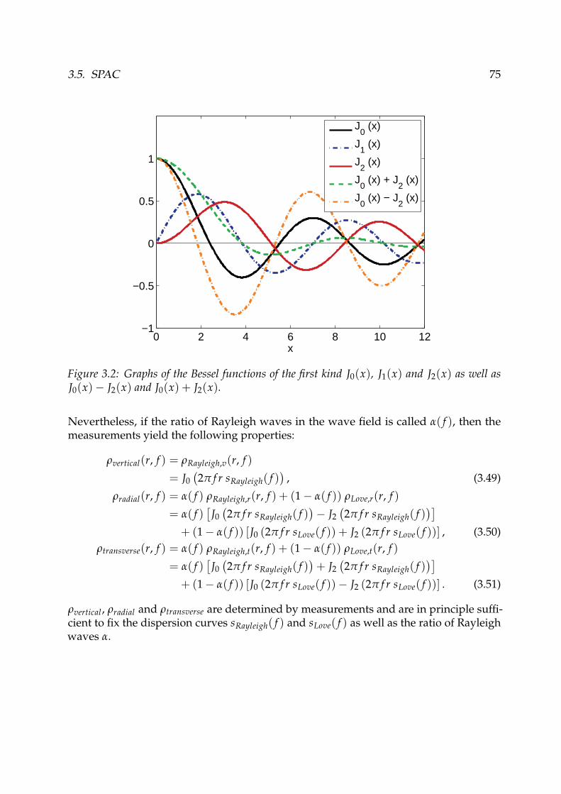
3.5. SPAC 75

0 2 4 6 8 10 12−1

−0.5

0

0.5

1

x

J

0 (x)

J1 (x)

J2 (x)

J0 (x) + J

2 (x)

J0 (x) − J

2 (x)

Figure 3.2: Graphs of the Bessel functions of the first kind J0(x), J1(x) and J2(x) as well asJ0(x)− J2(x) and J0(x) + J2(x).

Nevertheless, if the ratio of Rayleigh waves in the wave field is called α( f ), then themeasurements yield the following properties:

ρvertical(r, f ) = ρRayleigh,v(r, f )

= J0(2π f r sRayleigh( f )

), (3.49)

ρradial(r, f ) = α( f ) ρRayleigh,r(r, f ) + (1− α( f )) ρLove,r(r, f )

= α( f )[

J0(2π f r sRayleigh( f )

)− J2

(2π f r sRayleigh( f )

)]+ (1− α( f )) [J0 (2π f r sLove( f )) + J2 (2π f r sLove( f ))] , (3.50)

ρtransverse(r, f ) = α( f ) ρRayleigh,t(r, f ) + (1− α( f )) ρLove,t(r, f )

= α( f )[

J0(2π f r sRayleigh( f )

)+ J2

(2π f r sRayleigh( f )

)]+ (1− α( f )) [J0 (2π f r sLove( f ))− J2 (2π f r sLove( f ))] . (3.51)

ρvertical, ρradial and ρtransverse are determined by measurements and are in principle suffi-cient to fix the dispersion curves sRayleigh( f ) and sLove( f ) as well as the ratio of Rayleighwaves α.

76 CHAPTER 3. SEISMIC ARRAY METHODS

3.5.4 Applying the SPAC method

3.5.4.1 The Bessel functions

In figure 3.2, the Bessel functions of the first kind are plotted for the orders 0, 1 and 2.The calculation of the correlations between the central and the ring stations yields anoscillating function with decreasing amplitude. The roots of J0(x) are approximatelyx = 2.405, 5.520, 8.654, 11.792, . . . and the function has maxima at x = 0, 7.016, . . . andminima at x = 3.832, 10.174, . . .. Therefore, the equation J0(x) = y has multiple solu-tions if J0(3.832) < y < J0(7.016), which corresponds to x > 1.869. For the equationsJ0(x) + J2(x) and J0(x)− J2(x), the locations of the roots and extrema are different, butthe shape of the functions is comparable to J0(x). Regarding the problem of finding thedispersion curve, this means that for higher frequencies, multiple slowness values existwhich can explain the autocorrelation curve. Therefore, the use of autocorrelation curvesshould be limited to the first descending flank up to the first minimum of the curve.Additional measurements with different array radii can then be used to extend the inves-tigation to different frequency ranges. However, it is possible to make a direct inversionof the soil structure without trying to retrieve the dispersion curve first [Wathelet et al.,2005]. Then, in principle, the whole SPAC curve could be used, but in general the curvebeyond the second root is neither well constrained by the measurements (due to thearray layout) nor improving the inversion.

3.5.4.2 Practical problems

An application of the SPAC method as it was derived is in principle impossible as aninfinite number of seismic stations would be necessary so that the integration in equation(3.26) is mathematically possible. However, using less stations will still yield a curvewhich fits the Bessel function in an acceptable way. Formally, by using only N ringstations (regularly distributed on the ring of radius r), equation (3.26) transforms to

φ(r, f ) =1

2N ∑n

∑m

An( f )Am( f )N

∑l=1

cos(

k( f )r cos(

ϑm −2π l

N

))cos(ϕn − ϕm)

+1

2N ∑n

∑m

An( f )Am( f )N

∑l=1

sin(

k( f )r cos(

ϑm −2π l

N

))sin(ϕn − ϕm),

(3.52)

and

φ(0, f ) =12 ∑

n∑m

An( f )Am( f ) cos(ϕn − ϕm). (3.53)

3.5. SPAC 77

If we suppose different waves to be uncorrelated, equations (3.52) and (3.53) simplify to

φ(r, f ) =1

2N ∑n

A2n( f )

N

∑l=1

cos(

k( f )r cos(

ϑn −2π l

N

)), (3.54)

φ(0, f ) =12 ∑

nA2

n( f ). (3.55)

In order to investigate how close the theoretical response will be to the Bessel functiondepending on the number of stations, we will suppose that a single plane wave is incident(i.e. n = 1 and ϑn = ϑ) and that the N ring sensors are located regularly on a ring aroundthe central station. This yields

ρ(r, f , ϑ) =1N

N

∑l=1

cos(

k( f )r cos(

ϑ− 2π lN

)). (3.56)

In figure 3.3, the autocorrelation function given by equation (3.56) is computed for arraysof different sensor numbers, varying the azimuth. For comparison reasons, the Besselfunction J0(x) is also plotted. The first ring sensor is always placed exactly north of thecentral station. As the array is symmetric, the array responses of all azimuths can bereduced to the interval [0◦, ϑc], where ϑc = 360◦

4N if N is odd and ϑc = 360◦2N if N is even.

Therefore, the curves presented in figure 3.3 are displaying curves for ϑ varying from0 to ϑc, which are representative for all possible azimuths. In the figure, it can be seenthat for all curves the Bessel function is fitted up to a certain value x = xlimit whichdepends on the number of stations. For two ring stations, the SPAC method cannotwork if only waves from one azimuth arrive, which can also be seen in figure 3.3 (a). Forodd numbers of ring stations, xlimit is larger than for even numbers of ring stations ofcomparable size. Notably, the resolution for three ring stations (figure 3.3 (b)) is superiorthan for four ring stations (figure 3.3 (c)), etc. The curves for 3 and 6 ring stations and for5 and 10 ring stations are identical, respectively, because an array of 6 (10) sensors is builtfrom two sub-arrays of 3 (5) stations. For these examples, in the array with less sensors,every vector connecting a ring and the central station occurs only once. In the respectivearray with more sensors, every connection vector occurs twice, without improving theresolution. In this way, every array whose number of ring sensors is the double of anodd number, has the same resolution than the respective array with half the number ofstations. Actually, for every array of an even number of ring stations, an array with asmaller odd number and yet better resolution can be found.Examining odd and even ring station numbers separately, the resolution of the arrayincreases with the number of ring stations in both groups. Especially for the odd numbers,all arrays fit the Bessel function very well up to the first minimum at least. The three-station case resolves well up to the first minimum only, five stations up to the nextmaximum, seven stations up to the second minimum and so on. In this way, if themeasurements shall be accurate up to a certain degree, the odd number of stations whichare necessary to achieve this resolution can be given theoretically. Okada [2006] andCho et al. [2008] found similar results. In section 3.5.4.3, a mathematical proof will begiven illustrating that the Bessel function is fitted in a better way for an increasing (odd)number of ring stations.

78 CHAPTER 3. SEISMIC ARRAY METHODS

(a) (b) (c)

(d) (e) (f)

(g) (h) (i)

(j) (k)

Figure 3.3: Top: Theoretical autocorrelation functions for seismic arrays composed of a centralstation and between two and ten ring stations for different azimuths. The azimuth values rangefrom 0◦ to ϑc, with ϑc = 360◦

4N if N, the number of ring sensors, is odd and ϑc = 360◦2N if N is even.

Due to the symmetry of the respective array configurations, the value intervals are representativefor all possible azimuths. In the legends, only the extreme azimuth values are indicated, thedashed lines correspond to the intermediate azimuth values. Bottom: Theoretical autocorrelationfunctions for even (left) and odd (right) numbers of ring stations for a single incident wave withan azimuth of 0◦.

3.5. SPAC 79

Even though with a larger number of ring sensors the theoretical resolution of the arrayincreases, the non-uniqueness for values of x exceeding 1.869 subsists. This is whyactually, the first descending flank of the Bessel function is often the only measurementused for the retrieval of the dispersion curve. According to figure 3.3, with three seismicsensors the Bessel function can already be retrieved up to the first minimum. Further-more, the shown figures are obtained for a single incident wave, i.e. all wave energy isincident from a single azimuth. This is the worst possible scenario for using SPAC. Inreal case measurements, waves will be incident from all possible azimuths (principalazimuths with larger energy still being possible), and the results will correspond to amixture of the curves for different azimuths shown in figure 3.3. If the waves arrive fromall possible azimuths with the same energy (and different waves are uncorrelated), themeasurements will correspond to the average of the curves for all azimuths. Actually,the average curves for all array sizes in figure 3.3 coincide with the Bessel function.It should not be forgotten that the circular array layout with a central station is notmandatory. When using only the correlations between the central and the ring stations,the case of an array with three ring sensors surrounding a central station is indeedequivalent to the deployment of only three sensors forming an equilateral triangle. Nev-ertheless, the layout with a central station can be used to perform two distinguishedSPAC measurements with different distance and thus frequency ranges: The first onebetween the central station and the ring stations and the second between the differentring stations. Different, but equivalent array layouts can always be formed because theimportance lies in the distance vectors and not in the absolute positions.

3.5.4.3 Mathematical considerations relating to the number of seismic stations

In figure 3.3, it was shown that, for an odd number of ring stations, the Bessel function isfitted in a better way when increasing the number of seismic stations. Notably, whenusing 3 ring stations, the Bessel function was retrieved up to approximately the firstminimum, for 5 ring stations up to the next maximum, for 7 stations up to the nextminimum, and so on, independent of the azimuth of the incident wave.We found a mathematical proof for this which will be given in the following. For thesake of simplicity, we suppose that a single seismic wave is arriving under an azimuth of0◦. This is one of both extreme cases which deviate the most from the true Bessel curvein figure 3.3.The Bessel function J0(x) can be developed as a Taylor series, which yields

J0(x) =∞

∑k=0

akx2k, (3.57)

with

ak =(−1)k

22k(k!)2 . (3.58)

80 CHAPTER 3. SEISMIC ARRAY METHODS

In the same way, we define the function BN(x) = ρ(x, ϑ = 0), with ρ(x = k( f ) · r, ϑ)given by equation (3.56), where N is any odd number of seismic sensors on the ring:

BN(x) =1N

N

∑l=1

cos(

x cos(

2πlN

)). (3.59)

Using the Taylor series of the cosine functionIX, BN(x) can be developed as a Taylorseries as well:

BN(x) =1N

∞

∑k=0

(−1)k

(2k)!x2k

N

∑l=1

[cos

(2πlN

)]2k

=∞

∑k=0

bk x2k, (3.60)

with

bk =1N· (−1)k

(2k)!

N

∑l=1

[cos

(2πlN

)]2k. (3.61)

Applying the binomial theoremX to cosn x yields

cosn x =(

eix + e−ix

2

)n

=12n

n

∑k=0

(nk

)eix(n−2k). (3.62)

Now, bk can be written as

bk =1N· (−1)k

(2k)!

N

∑l=1

122k

2k

∑j=0

(2kj

)exp

(i2πlN

(2k− 2j))

. (3.63)

IXThe Taylor series of the cosine is given by

cos x =∞

∑k=0

(−1)kx2k

(2k)!.

XThe binomial theorem indicates the power of a binomial [Bronstein et al., 2001]:

(a + b)n =n

∑k=0

(nk

)an−kbk,

where(

nk

)= n!

k!(n−k)! is the binomial coefficient and x! is the factorial of x ∈N

defined by x! = x · (x− 1) · (x− 2) · · · 2 · 1.

3.5. SPAC 81

When calculating

N

∑l=1

exp(

i2πlN

(2k− 2j))

, (3.64)

two cases have to be considered separately.In the first case, k < N and therefore k− j < N. In this case, equation (3.64) equals zeroexcept if j = k. Then, equation (3.64) equals Nδjk and equation (3.63) simplifies to

bk =(−1)k

(2k)!1

22k(2k)!(k!)2 =

(−1)k

22k(k!)2 , (3.65)

which is equal to ak defined in equation (3.58).In the second case, k ≥ N. Consequently, as in equation (3.63) a summation over j occurs,at least two values of j will be found for which (k− j) is a multiple of N (e.g. for k = N,this is the case if j = 0 and j = 2N). Notably, if k = N, equation (3.64) gives the resultN(δjN + δj0 + δj,2N). Then, bN can be calculated as

bN =1N· (−1)N

(2N)!1

22N

2N

∑j=0

(2N

j

)N(δjN + δj0 + δj,2N)

=(−1)N

(2N)!1

22N

[(2N)!(N!)2 + 2

]= aN +

(−1)N

(2N)!1

22N−1 , (3.66)

which differs from ak defined by equation (3.58). This result is in agreement with theresults found by Okada [2006], using a different derivation.This proves that for a given odd number N of regularly distributed seismic sensors onthe ring, the SPAC measurement retrieves the Taylor series of the Bessel function up tothe k = 2(N − 1)th element. The terms for k ≥ N diverge from the terms of the Besselfunction and have larger absolute values. In other words, J0(x)− BN(x) = O(x2N). Thisexplains the results of figure 3.3. For N = 3, both curves’ coefficients are identical upto x4. Therefore, as the Bessel function is symmetrical (J0(−x) = J0(x)), the first tworoots (a negative and a positive one) are well fitted by B3(x) and the first minima areapproximately fitted as well. With each increment of N by 2, the agreement betweenJ0(x) and BN(x) increases of two additional terms and consequently the curves are inagreement for the next root and approximately up to the next extremum.

82 CHAPTER 3. SEISMIC ARRAY METHODS

3.5.5 Modified SPAC method (M-SPAC)The original SPAC method forces the seismic sensors to have equal distances one fromanother. When performing field measurements, however, this requirement is almostimpossible to fulfill. In urban areas in particular, buildings, infrastructure and plantshave to be accounted for when deploying the sensors. The classical method cannot beapplied there. Bettig et al. [2001] proposed the modified auto-correlation method (M-SPAC). This method allows the seismic sensors to be located in approximate rings or evencompletely different layouts. Sensor pairs of comparable distance are then assembledinto rings.

3.5.5.1 Vertical component

For the vertical component, grouping all sensor pairs with distances between r1 andr2 should yield an autocorrelation function which is the average function for all radiibetween r1 and r2. This average is calculated by integrating equation (3.29) for radiibetween r1 and r2 and renorming the result:

ρMSPAC,vertical(r1, r2, f ) =

r2∫r1

J0(2π f r s( f ))r dr

r2∫r1

r dr. (3.67)

By usingr∫

0J0(x)xdx = r J1(r), the integrals can be calculated:

r2∫r1

J0(2π f r s( f ))r dr =r2∫

0

J0(2π f r s( f ))r dr−r1∫

0

J0(2π f r s( f ))r dr

=1

4π2 f 2 s2( f )

r′2∫0

J0(r′)r′ dr′ −r′1∫

0

J0(r′)r′ dr′

=

14π2 f 2 s2( f )

[r′2 J1(r′2)− r′1 J1(r′1)

]=

12π f s( f )

[r2 J1(2π f r2 s( f ))− r1 J1(2π f r1 s( f ))] , (3.68)

r2∫r1

r dr =[

r2

2

]r2

r1

=r2

2 − r21

2. (3.69)

Inserting (3.68) and (3.69) in (3.67) yields

ρMSPAC,vertical(r1, r2, f ) =1

(r22 − r2

1)π f s( f )[r2 J1(2π f r2 s( f ))− r1 J1(2π f r1 s( f ))] .

(3.70)

3.5. SPAC 83

This is the theoretical formula. The measured correlations for all station pairs (i, j) withdistance rij comprised between r1 and r2 are weighted and averaged:

ρvertical(r1, r2, f ) =1π ∑

r1<rij<r2

ρ(rij, ϕij, f )∆ϕij, (3.71)

where ϕij indicates the angle under which station j is seen from station i or vice versa(0 < ϕij < π) and ∆ϕij (with ∑r1<rij<r2

∆ϕij = π) is a weighting factor which takesthe density of the distribution of sensor pairs at angle ϕij into account (if many stationpairs with comparable ϕ fall in the same ring, their respective weights are low). Theautocorrelations ρ(rij, ϕij, f ) for each station pair are calculated by

ρ(rij, ϕij, f ) =

∫ui,vertical( f , t)uj,vertical( f , t)dt√∫

u2i,vertical( f , t)dt

∫u2

j,vertical( f , t)dt. (3.72)

3.5.5.2 Horizontal components

The M-SPAC technique was extended to the horizontal components by Köhler et al. [2007].In analogy to the vertical component, the autocorrelation functions for the horizontalcomponents given by equations (3.50) and (3.51) are averaged over the radii between r1and r2:

ρMSPAC,radial(r, f ) =

r2∫r1

ρradial(r, f )r dr

r2∫r1

r dr, (3.73)

ρMSPAC,transverse(r, f ) =

r2∫r1

ρtransverse(r, f )r dr

r2∫r1

r dr. (3.74)

84 CHAPTER 3. SEISMIC ARRAY METHODS

By usingr2∫

r1

[J0(r)− J2(r)] r dr = 2 [J0(r2)− J0(r1) + r2 J1(r2)− r1 J1(r1)]

andr2∫

r1

[J0(r) + J2(r)] r dr = 2 [J0(r1)− J0(r2)], this finally leads to

ρMSPAC,radial(r, f ) =α( f )

r22 − r2

1

(1

π2 f 2 s2R( f )

[J0(2π f r2 sR( f ))− J0(2π f r1 sR( f ))]

+2

π f sR( f )[r2 J1(2π f r2 sR( f ))− r1 J1(2π f r1 sR( f ))]

)− 1− α( f )

(r22 − r2

1)π2 f 2s2L( f )

[J0(2πr2 f sL( f ))− J0(2πr1 f sL( f ))] ,

(3.75)

ρMSPAC,transverse(r, f ) =−α( f )

(r22 − r2

1)π2 f 2s2R( f )

[J0(2πr2 f sR( f ))− J0(2πr1 f sR( f ))]

+1− α( f )r2

2 − r21

(1

π2 f 2s2L( f )

[J0(2π f r2sL( f ))− J0(2π f r1sL( f ))]

+2

π f sL( f )[r2 J1(2π f r2sL( f ))− r1 J1(2π f r1sL( f ))]

),

(3.76)

where sR( f ) = sRayleigh( f ) and sL( f ) = sLove( f ). In analogy to the vertical component,the measured correlations for all station pairs (i, j) with r1 < rij < r2 are averaged andweighted to form the radial and transverse correlation functions

ρradial(r1, r2, f ) =1π ∑

r1<rij<r2

ρradial(rij, ϕij, f )∆ϕij, (3.77)

ρtransverse(r1, r2, f ) =1π ∑

r1<rij<r2

ρtransverse(rij, ϕij, f )∆ϕij, (3.78)

where ρradial and ρtransverse are calculated as in equation (3.72).

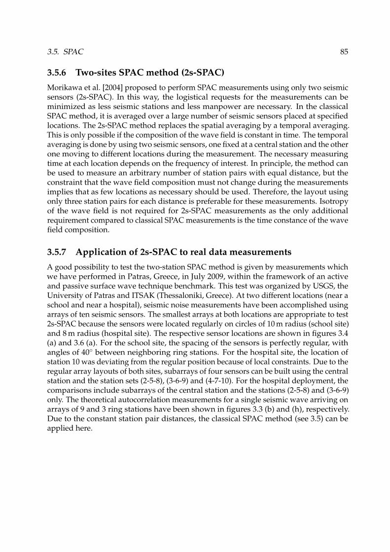
3.5. SPAC 85

3.5.6 Two-sites SPAC method (2s-SPAC)Morikawa et al. [2004] proposed to perform SPAC measurements using only two seismicsensors (2s-SPAC). In this way, the logistical requests for the measurements can beminimized as less seismic stations and less manpower are necessary. In the classicalSPAC method, it is averaged over a large number of seismic sensors placed at specifiedlocations. The 2s-SPAC method replaces the spatial averaging by a temporal averaging.This is only possible if the composition of the wave field is constant in time. The temporalaveraging is done by using two seismic sensors, one fixed at a central station and the otherone moving to different locations during the measurement. The necessary measuringtime at each location depends on the frequency of interest. In principle, the method canbe used to measure an arbitrary number of station pairs with equal distance, but theconstraint that the wave field composition must not change during the measurementsimplies that as few locations as necessary should be used. Therefore, the layout usingonly three station pairs for each distance is preferable for these measurements. Isotropyof the wave field is not required for 2s-SPAC measurements as the only additionalrequirement compared to classical SPAC measurements is the time constance of the wavefield composition.

3.5.7 Application of 2s-SPAC to real data measurements

A good possibility to test the two-station SPAC method is given by measurements whichwe have performed in Patras, Greece, in July 2009, within the framework of an activeand passive surface wave technique benchmark. This test was organized by USGS, theUniversity of Patras and ITSAK (Thessaloniki, Greece). At two different locations (near aschool and near a hospital), seismic noise measurements have been accomplished usingarrays of ten seismic sensors. The smallest arrays at both locations are appropriate to test2s-SPAC because the sensors were located regularly on circles of 10 m radius (school site)and 8 m radius (hospital site). The respective sensor locations are shown in figures 3.4(a) and 3.6 (a). For the school site, the spacing of the sensors is perfectly regular, withangles of 40◦ between neighboring ring stations. For the hospital site, the location ofstation 10 was deviating from the regular position because of local constraints. Due to theregular array layouts of both sites, subarrays of four sensors can be built using the centralstation and the station sets (2-5-8), (3-6-9) and (4-7-10). For the hospital deployment, thecomparisons include subarrays of the central station and the stations (2-5-8) and (3-6-9)only. The theoretical autocorrelation measurements for a single seismic wave arriving onarrays of 9 and 3 ring stations have been shown in figures 3.3 (b) and (h), respectively.Due to the constant station pair distances, the classical SPAC method (see 3.5) can beapplied here.

86 CHAPTER 3. SEISMIC ARRAY METHODS

3.5.7.1 Location near the school

(a)

−10 −5 0 5 10

−10

−5

0

5

10

12

3

4

5

6

7

8 9

10

Distance [m]

Dis

tanc

e [m

]

(b)

5 10 15 20 25 30 35 40−0.75

−0.5

−0.25

0

0.25

0.5

0.75

1

Frequency [Hz]

Aut

ocor

rela

tion

Vertical component

(c)

5 10 15 20 25 30 35 40−0.75

−0.5

−0.25

0

0.25

0.5

0.75

1

Frequency [Hz]

Aut

ocor

rela

tion

Radial component

(d)

5 10 15 20 25 30 35 40−0.75

−0.5

−0.25

0

0.25

0.5

0.75

1

Frequency [Hz]A

utoc

orre

latio

n

Transverse component

(e)

5 10 15 20 25 30 35 40−0.5

−0.25

0

0.25

0.5

0.75

1

Frequency [Hz]

Aut

ocor

rela

tion

Vertical component

10s−SPAC4s−SPAC (2−5−8)4s−SPAC (3−6−9)4s−SPAC (4−7−10)

(f)

5 10 15 20 25 30 35 40−0.5

−0.25

0

0.25

0.5

0.75

1

Frequency [Hz]

Aut

ocor

rela

tion

Radial component

10s−SPAC4s−SPAC (2−5−8)4s−SPAC (3−6−9)4s−SPAC (4−7−10)

(g)

5 10 15 20 25 30 35 40−0.5

−0.25

0

0.25

0.5

0.75

1

Frequency [Hz]

Aut

ocor

rela

tion

Transverse component

10s−SPAC4s−SPAC (2−5−8)4s−SPAC (3−6−9)4s−SPAC (4−7−10)

Figure 3.4: (a) Layout of the seismic array and definition of the different subarrays (all subarraysinclude the central station). Autocorrelation function between the central and all ring stations for(b) the vertical, (c) the radial and (d) the transverse component. Comparison between the averageautocorrelation curve using all ten stations simultaneously (10s-SPAC, using 9 station pairsbetween the central and the ring stations) and the three subarrays (4s-SPAC, using 3 station pairsbetween the central and ring stations) for (e) the vertical, (f) the radial and (g) the transversecomponent.

The array layout of the measurements performed near the school is shown in figure 3.4(a). The total duration of simultaneous seismic signal recordings is 45 minutes. Themeasured autocorrelation functions for every station pair consisting of the central anda ring station are shown in figures 3.4 (b) - (d) for the vertical, radial and transversecomponents, respectively. If the seismic noise wave field had been completely isotropic,the autocorrelation function for every seismic sensor pair should be the same.

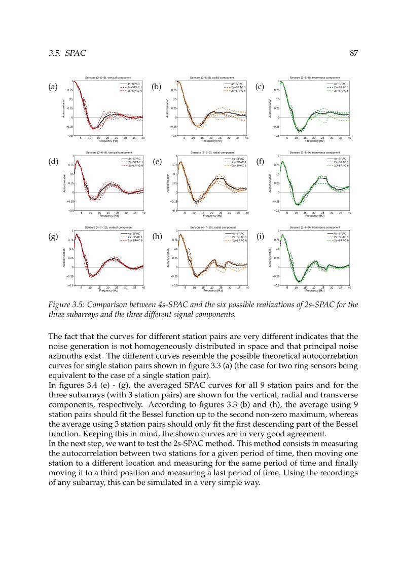
3.5. SPAC 87

(a)

5 10 15 20 25 30 35 40−0.5

−0.25

0

0.25

0.5

0.75

1

Frequency [Hz]

Aut

ocor

rela

tion

Sensors (2−5−8), vertical component

4s−SPAC2s−SPAC 12s−SPAC 6

(b)

5 10 15 20 25 30 35 40−0.5

−0.25

0

0.25

0.5

0.75

1

Frequency [Hz]

Aut

ocor

rela

tion

Sensors (2−5−8), radial component

4s−SPAC2s−SPAC 12s−SPAC 6

(c)

5 10 15 20 25 30 35 40−0.5

−0.25

0

0.25

0.5

0.75

1

Frequency [Hz]

Aut

ocor

rela

tion

Sensors (2−5−8), transverse component

4s−SPAC2s−SPAC 12s−SPAC 6

(d)

5 10 15 20 25 30 35 40−0.5

−0.25

0

0.25

0.5

0.75

1

Frequency [Hz]

Aut

ocor

rela

tion

Sensors (3−6−9), vertical component

4s−SPAC2s−SPAC 12s−SPAC 6

(e)

5 10 15 20 25 30 35 40−0.5

−0.25

0

0.25

0.5

0.75

1

Frequency [Hz]

Aut

ocor

rela

tion

Sensors (3−6−9), radial component

4s−SPAC2s−SPAC 12s−SPAC 6

(f)

5 10 15 20 25 30 35 40−0.5

−0.25

0

0.25

0.5

0.75

1

Frequency [Hz]

Aut

ocor

rela

tion

Sensors (3−6−9), transverse component

4s−SPAC2s−SPAC 12s−SPAC 6

(g)

5 10 15 20 25 30 35 40−0.5

−0.25

0

0.25

0.5

0.75

1

Frequency [Hz]

Aut

ocor

rela

tion

Sensors (4−7−10), vertical component

4s−SPAC2s−SPAC 12s−SPAC 6

(h)

5 10 15 20 25 30 35 40−0.5

−0.25

0

0.25

0.5

0.75

1

Frequency [Hz]

Aut

ocor

rela

tion

Sensors (4−7−10), radial component

4s−SPAC2s−SPAC 12s−SPAC 6

(i)

5 10 15 20 25 30 35 40−0.5

−0.25

0

0.25

0.5

0.75

1

Frequency [Hz]

Aut

ocor

rela

tion

Sensors (3−6−9), transverse component

4s−SPAC2s−SPAC 12s−SPAC 6

Figure 3.5: Comparison between 4s-SPAC and the six possible realizations of 2s-SPAC for thethree subarrays and the three different signal components.

The fact that the curves for different station pairs are very different indicates that thenoise generation is not homogeneously distributed in space and that principal noiseazimuths exist. The different curves resemble the possible theoretical autocorrelationcurves for single station pairs shown in figure 3.3 (a) (the case for two ring sensors beingequivalent to the case of a single station pair).In figures 3.4 (e) - (g), the averaged SPAC curves for all 9 station pairs and for thethree subarrays (with 3 station pairs) are shown for the vertical, radial and transversecomponents, respectively. According to figures 3.3 (b) and (h), the average using 9station pairs should fit the Bessel function up to the second non-zero maximum, whereasthe average using 3 station pairs should only fit the first descending part of the Besselfunction. Keeping this in mind, the shown curves are in very good agreement.In the next step, we want to test the 2s-SPAC method. This method consists in measuringthe autocorrelation between two stations for a given period of time, then moving onestation to a different location and measuring for the same period of time and finallymoving it to a third position and measuring a last period of time. Using the recordingsof any subarray, this can be simulated in a very simple way.

88 CHAPTER 3. SEISMIC ARRAY METHODS

As the total recording length is 45 minutes, we will calculate the autocorrelation using thefirst 15 minutes of signal for the central and the first ring station, the second 15 minutesof signal for the central and the second ring station and finally the third 15 minutes forthe pair involving the third ring station.In this way, using a single subarray, six different 2s-SPAC measurements can be simulated,depending on which ring station is the first, second and third one. The results of thisprocedure are given in figure 3.5. Figures 3.5 (a) - (c) give the results for using thesubarray (2-5-8) for the vertical, radial and transverse components, respectively, (d)- (f) for the subarray (3-6-9) and (g) - (i) for the subarray (4-7-10). According to thetheoretical considerations of figure 3.3, the measurements should fit the correct Besselfunction up to the first minimum only. In this frequency range and apart from someminor discrepancies, the 2s-SPAC curves are in very good agreement with the classicalSPAC curves using all four stations at the same time (4s-SPAC) for every combination ofsubarray and component. The non-isotropy of the noise wave field does not constitute aproblem for the 2s-SPAC measurements. Besides, the fact that the 2s-SPAC measurementsagree with the 4s-SPAC measurements indicates that the constitution of the seismic noisewave field did not change during the 45 minutes of measurement.

3.5.7.2 Location near the hospital

For the measurements at the location near the hospital, the array layout is given in figure3.6 (a). At this location, 60 minutes of seismic signals have been recorded simultaneouslyon all stations. Figures 3.6 (b) - (d) show the autocorrelation functions for every stationpair consisting of the central and a ring station. Here again, the noise wave field is notperfectly isotropic. Figures 3.6 (e) - (g) indicate the average autocorrelation functionsusing 9 seismic sensors and two subarrays of 4 sensors. As sensor 10 could not beplaced on the exact location necessary for the regular array, it was placed about a meteraside. Therefore, this station is disregarded in the following. For all components, themeasurements using only 4 stations are comparable with the measurements includingall stations, but the respective curves are far away from being Bessel functions. Theresults for the six possible realizations of a simulated 2s-SPAC are shown for one of bothsubarrays only in figures 3.6 (h) - (j). For the other subarray, the results are comparable.For 2s-SPAC, the curves do not look like a Bessel function neither, but are still close tothe 4s-SPAC using the same data. The strange autocorrelation curves could be linked tothe presence of higher modes in the wave field or a too narrow seismic sensor spacing.In fact, if the wave velocity is high and the sensors are too closely located, it can happenthat the SPAC measurements at higher frequencies deviate from the Bessel function.

3.5. SPAC 89

(a)

−10 −5 0 5 10

−5

0

5

1

2

34

5

6

7

8

9

10

Distance [m]

Dis

tanc

e [m

]

(b)

5 10 15 20 25 30 35 40−0.75

−0.5

−0.25

0

0.25

0.5

0.75

1

Frequency [Hz]

Aut

ocor

rela

tion

Vertical component

(c)

5 10 15 20 25 30 35 40−0.75

−0.5

−0.25

0

0.25

0.5

0.75

1

Frequency [Hz]

Aut

ocor

rela

tion

Radial component

(d)

5 10 15 20 25 30 35 40−0.75

−0.5

−0.25

0

0.25

0.5

0.75

1

Frequency [Hz]

Aut

ocor

rela

tion

Transverse component

(e)

5 10 15 20 25 30 35 40−0.5

−0.25

0

0.25

0.5

0.75

1

Frequency [Hz]

Aut

ocor

rela

tion

Vertical component

9s−SPAC4s−SPAC (2−5−8)4s−SPAC (3−6−9)

(f)

5 10 15 20 25 30 35 40−0.5

−0.25

0

0.25

0.5

0.75

1

Frequency [Hz]

Aut

ocor

rela

tion

Radial component

9s−SPAC4s−SPAC (2−5−8)4s−SPAC (3−6−9)

(g)

5 10 15 20 25 30 35 40−0.5

−0.25

0

0.25

0.5

0.75

1

Frequency [Hz]

Aut

ocor

rela

tion

Transverse component

9s−SPAC4s−SPAC (2−5−8)4s−SPAC (3−6−9)

(h)

5 10 15 20 25 30 35 40−0.5

−0.25

0

0.25

0.5

0.75

1

Frequency [Hz]

Aut

ocor

rela

tion

Sensors (3−6−9), vertical component

4s−SPAC2s−SPAC 12s−SPAC 6

(i)

5 10 15 20 25 30 35 40−0.5

−0.25

0

0.25

0.5

0.75

1

Frequency [Hz]

Aut

ocor

rela

tion

Sensors (3−6−9), radial component

4s−SPAC2s−SPAC 12s−SPAC 6

(j)

5 10 15 20 25 30 35 40−0.5

−0.25

0

0.25

0.5

0.75

1

Frequency [Hz]

Aut

ocor

rela

tion

Sensors (3−6−9), transverse component

4s−SPAC2s−SPAC 12s−SPAC 6

Figure 3.6: (a) Layout of the seismic array and definition of the different subarrays (all subarraysinclude the central station). Autocorrelation function between the central and all ring stations(except station 10) for (b) the vertical, (c) the radial and (d) the transverse component. Comparisonbetween the average autocorrelation curves using the 8 station pairs between the central and thering stations simultaneously (9s-SPAC) and the two subarrays (4s-SPAC, using 3 station pairsbetween the central and ring stations) for (e) the vertical, (f) the radial and (g) the transversecomponent. (h-j) Comparison between 4s-SPAC and the six possible realizations of 2s-SPAC forthe subarray (3-6-9) and the three different signal components.

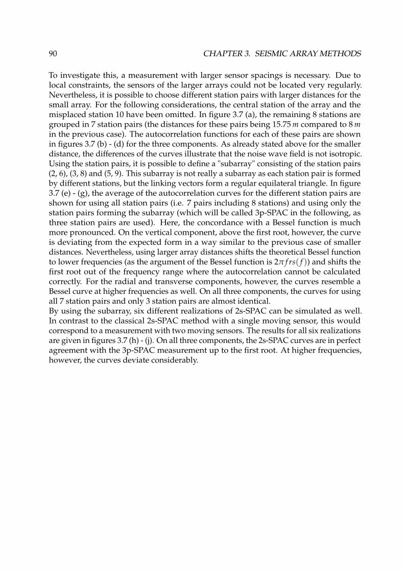
90 CHAPTER 3. SEISMIC ARRAY METHODS

To investigate this, a measurement with larger sensor spacings is necessary. Due tolocal constraints, the sensors of the larger arrays could not be located very regularly.Nevertheless, it is possible to choose different station pairs with larger distances for thesmall array. For the following considerations, the central station of the array and themisplaced station 10 have been omitted. In figure 3.7 (a), the remaining 8 stations aregrouped in 7 station pairs (the distances for these pairs being 15.75 m compared to 8 min the previous case). The autocorrelation functions for each of these pairs are shownin figures 3.7 (b) - (d) for the three components. As already stated above for the smallerdistance, the differences of the curves illustrate that the noise wave field is not isotropic.Using the station pairs, it is possible to define a "subarray" consisting of the station pairs(2, 6), (3, 8) and (5, 9). This subarray is not really a subarray as each station pair is formedby different stations, but the linking vectors form a regular equilateral triangle. In figure3.7 (e) - (g), the average of the autocorrelation curves for the different station pairs areshown for using all station pairs (i.e. 7 pairs including 8 stations) and using only thestation pairs forming the subarray (which will be called 3p-SPAC in the following, asthree station pairs are used). Here, the concordance with a Bessel function is muchmore pronounced. On the vertical component, above the first root, however, the curveis deviating from the expected form in a way similar to the previous case of smallerdistances. Nevertheless, using larger array distances shifts the theoretical Bessel functionto lower frequencies (as the argument of the Bessel function is 2π f rs( f )) and shifts thefirst root out of the frequency range where the autocorrelation cannot be calculatedcorrectly. For the radial and transverse components, however, the curves resemble aBessel curve at higher frequencies as well. On all three components, the curves for usingall 7 station pairs and only 3 station pairs are almost identical.By using the subarray, six different realizations of 2s-SPAC can be simulated as well.In contrast to the classical 2s-SPAC method with a single moving sensor, this wouldcorrespond to a measurement with two moving sensors. The results for all six realizationsare given in figures 3.7 (h) - (j). On all three components, the 2s-SPAC curves are in perfectagreement with the 3p-SPAC measurement up to the first root. At higher frequencies,however, the curves deviate considerably.

3.5. SPAC 91

(a)

−10 −5 0 5 10

−5

0

5

1

10

2

34

5

6

7

8

9

Distance [m]

Dis

tanc

e [m

]

(b)

5 10 15 20 25 30 35 40−0.75

−0.5

−0.25

0

0.25

0.5

0.75

1

Frequency [Hz]

Aut

ocor

rela

tion

Vertical component

(c)

5 10 15 20 25 30 35 40−0.75

−0.5

−0.25

0

0.25

0.5

0.75

1

Frequency [Hz]

Aut

ocor

rela

tion

Radial component

(d)

5 10 15 20 25 30 35 40−0.75

−0.5

−0.25

0

0.25

0.5

0.75

1

Frequency [Hz]

Aut

ocor

rela

tion

Transverse component

(e)

5 10 15 20 25 30 35 40−0.5

−0.25

0

0.25

0.5

0.75

1

Frequency [Hz]

Aut

ocor

rela

tion

Vertical component

8s−SPAC3p−SPAC (f)

5 10 15 20 25 30 35 40−0.5

−0.25

0

0.25

0.5

0.75

1

Frequency [Hz]

Aut

ocor

rela

tion

Radial component

8s−SPAC3p−SPAC (g)

5 10 15 20 25 30 35 40−0.5

−0.25

0

0.25

0.5

0.75

1

Frequency [Hz]

Aut

ocor

rela

tion

Transverse component

8s−SPAC3p−SPAC

(h)

5 10 15 20 25 30 35 40−0.5

−0.25

0

0.25

0.5

0.75

1

Frequency [Hz]

Aut

ocor

rela

tion

Vertical component

3p−SPAC2s−SPAC 12s−SPAC 6

(i)

5 10 15 20 25 30 35 40−0.5

−0.25

0

0.25

0.5

0.75

1

Frequency [Hz]

Aut

ocor

rela

tion

Radial component

3p−SPAC2s−SPAC 12s−SPAC 6

(j)

5 10 15 20 25 30 35 40−0.5

−0.25

0

0.25

0.5

0.75

1

Frequency [Hz]

Aut

ocor

rela

tion

Transverse component

3p−SPAC2s−SPAC 12s−SPAC 6

Figure 3.7: (a) Layout of the seismic array and definition of subarray (orange). Autocorrelationfunction for the pairs of stations indicated in (a) for (b) the vertical, (c) the radial and (d) thetransverse component. Comparison between the average autocorrelation curves using all 7 stationpairs (8s-SPAC) and the subarray (3p-SPAC, using the 3 orange station pairs) for (e) the vertical,(f) the radial and (g) the transverse component. (h-i) Comparison between 3p-SPAC and the sixpossible realizations of 2s-SPAC for the orange subarray and the three different signal components.

92 CHAPTER 3. SEISMIC ARRAY METHODS

3.6 Conclusion

In this chapter, important methods to characterize seismic waves using arrays of sensorshave been presented. Of course, many more methods exist [Marcos, 1998], which havenot been presented here. The first presented methods (i.e. beamforming, frequency-wavenumber analysis and MUSIQUE) allow the estimation of an incident wave vector(i.e. the estimation of azimuth and velocity), whereas SPAC only allows the estimation ofthe velocity.

Theoretical considerations of the SPAC method demonstrated that an odd number ofring stations is always preferable to an even number of ring stations. Indeed, the classicallayout with a ring of sensors surrounding a central station itself is not essential. Byomitting the central station, the ring stations still form the same number of station pairsat each distance value. For example, an array of 3 stations surrounding a central stationcan be replaced by a smaller array of 3 stations only, positioned in a way to form anequilateral triangle. Nevertheless, for the layout including the central station, SPACmeasurements for two different distance values are obtained.

The tests of the 2s-SPAC method did not show significant differences between SPACmeasurements including 9 station pairs, 3 station pairs or 2s-SPAC. The 2s-SPAC methodis therefore an interesting means of characterizing the wave field with the least possiblemeasurement effort. The only additional prerequisite of the method is the temporalstationarity of the wave field. However, when performing a real 2s-SPAC measurement,this property can not be estimated easily. If the wave field composition changes duringthe measurement, the measured energy at the reference station is likely to change, too.However, it is still possible that the energy of the wave field stays constant, but theprincipal source azimuths change. A fourth measurement at the same location as thefirst one could affirm the temporal stationarity of the signals. To assure the temporalstationarity of the wave field, the measurement times of the 2s-SPAC method should bekept as short as possible.

SPAC measurements will be used to fix the absolute values of the velocities in the soilmodel in joint inversions with ellipticity curves: In chapter 6, the theoretical aspects ofjoint inversions of Rayleigh wave ellipticity and SPAC curves are investigated, beforethe results are applied to real data measurements in chapter 7.In chapter 4, advanced versions of the MUSIC algorithm using quaternions or biquater-nions are presented. This will then lead to the development of the MUSIQUE algorithm.

Chapter 4

Advanced seismic array methods usinghypercomplex numbers

This chapter is dedicated to array methods which use hypercomplex numbers. First, theproperties of quaternions and biquaternions, two examples of hypercomplex numbers,are indicated. Then, versions of the MUSIC algorithm exploiting these properties toretrieve the polarization parameters between different signal components are presented.Finally, the MUSIQUE algorithm is developed, which combines the classical MUSICalgorithm with a quaternion-MUSIC algorithm and allows the estimation of azimuth andvelocity, the identification of Love and Rayleigh waves and the polarization estimationfor Rayleigh waves.

Ce chapitre est dédié aux méthodes de réseau utilisant des nombres hypercomplexes. Dans unpremier temps, les propriétés de quaternions et de biquaternions, deux exemples de nombreshypercomplexes, seront indiquées. Après, des versions de l’algorithme MUSIC tirant profitdes propriétés de ces nombres pour retrouver la polarisation entre différentes composantes dusignal seront présentées. Ceci mènera finalement au développement de l’algorithme MUSIQUE,une combinaison de l’algorithme classique avec l’algorithme quaternionique de MUSIC. Cetalgorithme permet l’estimation d’azimut et de vitesse ainsi que l’identification d’ondes de Loveet de Rayleigh et l’estimation de la polarisation de ces dernières.

93

94 CHAPTER 4. HYPERCOMPLEX ARRAY METHODS

4.1 Introduction

In section 3.4, the original MUSIC algorithm [Schmidt, 1986] was presented. This codedeals with monocomponent signals only and is not particularly designed for multicom-ponent signals. Therefore, three-component signals can be either analyzed for each signalcomponent separately or by putting the signals of the different components in a singledata vector. However, the polarization information between the different components islost in both cases. To keep the polarization relations between the different components,their respective data have to be stored separately. The MUSIC data matrix for a singlecomponent is complex valued. In order to store multiple components in a single datamatrix, hypercomplex numbers can be used.

Examples of hypercomplex numbers are the quaternions (of dimension 4) and the bi-quaternions (of dimension 8). In this way, two complex-valued data matrices correspond-ing to different components can be stored in a single quaternion-valued data matrix orall three components of the seismic signals can be stored in a single biquaternion matrix.In fact, MUSIC versions using quaternions have been proposed by Miron et al. [2005b,2006] and using biquaternions by Miron [2005].

This chapter starts with presenting the properties of quaternions and biquaternionswhich are necessary to understand the respective MUSIC versions (sections 4.2 and 4.3).In section 4.4, the original methodology of quaternion-MUSIC [Miron et al., 2006] isindicated. We show that in contrast to the original method, it is not necessary to performa grid search to determine the two polarization parameters of a two-component wave(i.e. amplitude ratio and phase difference) if the wave vector (azimuth and velocity) isalready known. In this case, the polarization parameters can be obtained analytically.Then, in section 4.5, the biquaternion version of MUSIC as proposed by Miron [2005] ispresented. Here again, we show that the grid search for the four polarization parametersdescribing three-component waves (two amplitude ratios and two phase differences) canbe largely simplified if the wave vector has been previously determined. However, wealso show that the biquaternion approach fails in basic cases as identical signals on twoor three components or two-dimensional signals.

These considerations finally lead to the development of MUSIQUE, which combines theclassical MUSIC algorithm and the quaternion-MUSIC algorithm. MUSIQUE is designedto determine azimuth and velocity of incident waves, identify Love and possible Rayleighwaves and estimate the polarization parameters (among them ellipticity) of possibleRayleigh waves. The algorithm is presented in section 4.6.

4.2. QUATERNIONS 95

4.2 Quaternions

Quaternions are an extension of the complex numbers and have been discovered by theIrish mathematician Sir William Rowan Hamilton in 1843I(Hamilton [1844-50]). In fact,the French mathematician Olinde Rodrigues had already used quaternions in 1840 todescribe rotations in 3-dimensional space (Rodrigues [1840]), but indeed without callingthem quaternions. Later, his work fell into oblivion. Kantor and Solodovnikov [1989]give a good overview of quaternion algebra and Sweetser [2005] demonstrates how theuse of quaternions can simplify basic equations in physics. Using quaternions, rotationscan be calculated faster than using rotation matrices. Therefore, the use of quaternionsincludes video cards in modern computers. Here, only the basic rules of quaternionalgebra which are necessary to understand the following section will be presented.

4.2.1 Definition

A quaternion is defined as

q = q0 + q1 i+ q2 j+ q3 k, (4.1)

where q0, . . . , q3 ∈ R and i, j and k are imaginary units defined by

i2 = j2 = k2 = ijk = −1 (4.2)

q0 is called scalar part of the quaternion and q1 i+ q2 j+ q3 k forms the vector part. Theset of all quaternions is denoted by H. Based on the equations (4.2), it follows that

ij = k, ji = −kjk = i, kj = −i (4.3)ki = j, ik = −j

Evidently, the multiplication of quaternions is not commutative.

IAfter spending many years on the fruitless quest for a three-dimensional extension of the complexnumbers, in 1843, while on a walk with his wife, Hamilton got suddenly struck by the idea of a four-dimensional extension, the quaternions. As he was crossing the Broom Bridge in Dublin, Ireland, heimmediately carved the fundamental formula defining quaternions into the bridge. Today, a plaque on thebridge commemorates this event. Its inscription says:

"Here as he walked byon the 16th of October 1843

Sir William Rowan Hamiltonin a flash of genius discoveredthe fundamental formula for

quaternion multiplicationi2 = j2 = k2 = ijk = −1

& cut it on a stone of this bridge"

96 CHAPTER 4. HYPERCOMPLEX ARRAY METHODS

4.2.2 PropertiesBe p and q ∈H given by

p = p0 + p1 i+ p2 j+ p3 k, (4.4)q = q0 + q1 i+ q2 j+ q3 k. (4.5)

The addition of quaternions is then defined by

p + q = (p0 + q0) + (p1 + q1) i+ (p2 + q2) j+ (p3 + q3) k. (4.6)

From equations (4.3), it follows that the multiplication of p and q yields

pq =(p0q0 − p1q1 − p2q2 − p3q3) + (p0q1 + p1q0 + p2q3 − p3q3) i+ (p0q2 − p1q3 + p2q0 + p3q1) j+ (p0q3 + p1q2 − p2q1 + p3q0) k. (4.7)

It can be seen from equations (4.6) and (4.7) that the addition of quaternions is commu-tative, whereas the multiplication, in general, is not: p q 6= q p. However, quaternionmultiplication is still associative, i.e.

(p q) r = p (q r) (4.8)

for any p, q, r ∈H, which can be easily shown by direct calculation.In analogy to the complex numbers, the conjugate of a quaternion q = q0 + q1 i+ q2 j+q3 k is defined by

q∗ = q0 − q1 i− q2 j− q3 k. (4.9)

By using equation (4.7), it can be shown that the product of q with its conjugate q∗ isgiven by

qq∗ = q∗q = q20 + q2

1 + q22 + q2

3. (4.10)

In this way, the norm or absolute value of a quaternion can be defined by

|q| =√

q∗q =√

q20 + q2

1 + q22 + q2

3. (4.11)

The inverse value of a quaternion q 6= 0 is given by

q−1 =q∗

|q| . (4.12)

The quaternion division is defined in this way, too.We define the functions S(q), I(q), J(q) and K(q), which extract the different parts of thequaternion q defined in equation (4.1), by:

S(q) =q + q∗

2= q0, (4.13)

I(q) =i (q− q∗) + (q− q∗) i

−4= q1, (4.14)

J(q) =j (q− q∗) + (q− q∗) j

−4= q2, (4.15)

K(q) =k (q− q∗) + (q− q∗) k

−4= q3. (4.16)

4.2. QUATERNIONS 97

4.2.3 Cayley-Dickson representationAn arbitrary quaternion q = q0 + q1 i+ q2 j+ q3 k can be written in the form

q = (q0 + q1 i) + (q2 + q3 i) j = z0 + z1 j, (4.17)

where z1 and z2 ∈ C. In this way, a quaternion can be represented as a complex numberwith complexified coefficients. This is called the Cayley-Dickson representation.

4.2.4 Quaternion vectors

A quaternion vector~q ∈HN is an N-dimensional vector whose elements are quaternions.For two vectors ~q,~p ∈HN, the inner product is given by (e.g. Miron [2005])

〈~p | ~q〉 = ~q†~p, (4.18)

where ~q† =(~qT)∗ denotes the conjugate transpose of a quaternion vector.

The norm of a quaternion vector can then be defined by

‖~q‖ =√〈~q | ~q〉 =

√~q†~q. (4.19)

The set of quaternion-valued vectors forms a Hilbert spaceII. Two quaternion vectors~q,~p ∈HN are orthogonal if their inner product equals zero:

〈~p | ~q〉 = 0. (4.20)

IIA quaternion Hilbert space H is a complete metric space with respect to the distance function inducedby the inner product. This means that for every ~p, ~q,~r ∈ H and α, β ∈H, the following properties are true:

• (~p +~q) ∈ H, (α~p) ∈ H, α(β~p) = (αβ)~p.

• An inner product 〈~p | ~q〉 is defined with:〈~q | ~q〉 ∈ R+

0 , 〈~q | ~q〉 = 0 iff ~q =~0,〈~pα +~qβ |~r〉 = 〈~p |~r〉α + 〈~q |~r〉β〈~p | ~q〉 = 〈~q | ~p〉∗.

• H is complete, i.e. every Cauchy sequence in H converges in H.

98 CHAPTER 4. HYPERCOMPLEX ARRAY METHODS

4.2.5 Quaternion matrices

As quaternions are not commutative, the properties of quaternion matrices differ fromreal or complex matrices. Considering a quaternion matrix A ∈HM×N, we will denoteby AT the transpose, by A∗ the conjugate and by A† the conjugatee transpose of A.A good overview of quaternion matrices is given by Zhang [1997]. In the following,some results of this article will be presented. In particular, for two quaternion matricesA ∈HM×N and B ∈HN×O, the following properties hold:

1. (A∗)T = (AT)∗

2. (A B)† = B† A†

3. (A B)∗ 6= A∗ B∗, in general

4. (A B)T 6= BT AT, in general

5. (A B)−1 = B−1 A−1, if A and B are invertible

6. (A†)−1 = (A−1)†, if A is invertible

7. (A∗)−1 6= (A−1)∗, in general

8. (AT)−1 6= (A−1)T, in general

Due to the non-commutativity of quaternions, a quaternion matrix A ∈ HN×N has rightand left eigenvalues, satisfying the equations

A~ur = ~urλr, (4.21)A~ul = λl~ul, (4.22)

respectively. In general, both eigenvalues are different. The theory of left eigenvaluesis not yet well understood in literature, but the properties of right eigenvalues are wellestablished Zhang [1997]. Therefore, in the following, we will use exclusively righteigenvalues and eigenvectors.In analogy to the Cayley-Dickson representation of quaternions (equation 4.17), anyquaternion matrix A ∈ HN×N can be written as a combination of two complex matricesA1, A2 ∈ HN×N by A = A1 + A2j, as well as every vector ~u ∈ HN can be written as~u = ~u1 + ~u2j. Now, the eigenvalue equation (4.21) can be written as

(A1 + A2j)(~u1 + ~u2j) = (~u1 + ~u2j)λ (4.23)A1~u1 −A2~u∗2 + (A1~u2 + A2~u∗1)j = λ~u1 + λ∗~u2j, (4.24)

which is equivalent to the equations

A1~u1 −A2~u∗2 = λ~u1, (4.25)A1~u2 + A2~u∗1 = λ∗~u2. (4.26)

4.2. QUATERNIONS 99

Conjugation of equations (4.25) and (4.26) yields

A∗1~u∗1 −A∗2~u2 = λ∗~u∗1 , (4.27)

A∗1~u∗2 + A∗2~u1 = λ~u∗2 . (4.28)

Finally, equations (4.25) and (4.28) can be combined in matrix form as(A1 A2−A∗2 A∗1

)(~u1−~u∗2

)= λ

(~u1−~u∗2

), (4.29)

and equations (4.26) and (4.27) combine to(A1 A2−A∗2 A∗1

)(~u2~u∗1

)= λ∗

(~u2~u∗1

). (4.30)

The matrix χA =(

A1 A2−A∗2 A∗1

)∈ C2N×2N is called adjoint matrix of A.

χA has 2N eigenvectors with 2N associated (complex) eigenvalues. According to equa-tions (4.29) and (4.30), if λ is an eigenvalue of χA, λ∗ is also an eigenvalue. This meansthat the eigenvalues of χA occur in conjugated pairs. On the other side, according toequations (4.29) and (4.30), every eigenvalue of χA is also an eigenvalue of A.If λ is an eigenvalue of A, then ρ−1λρ is an eigenvalue as well [Brenner, 1951]: AsA~u = ~uλ, it follows that A(~uρ) = (~uρ)ρ−1λρ. Therefore, (~uρ) is an eigenvector corre-sponding to the eigenvalue ρ−1λρ.Notably, setting ρ = j or ρ = k yields ρ−1λρ = λ∗. Therefore, if ~uλ and ~uλ∗ are theeigenvectors corresponding to λ and λ∗, respectively, it follows that ~uλj and ~uλk arealso eigenvectors of A. In this way, an infinite number of eigenvalue and eigenvectorpairs of A can be generated based on a single (complex) eigenvalue λ0 by using anyquaternion-valued ρ, which yields λ′ = ρ−1λρ and ~u′ = ~uρ. However, all these eigen-vectors are not independent among each other and form a class of eigenvalues. Notably,the eigenvectors ~uλ and ~uλ∗ of equations (4.29) and (4.30) are not linearly independentand λ and λ∗ correspond to the same eigenvalue class of A. If χA has real eigenvalues,however, the application of ρ−1λρ does not change λ and consequently, this eigenvalueof χA occurs twice.The matrix A has only N linearly independent eigenvectors. By taking one eigenvalueof χA per eigenvalue class, the corresponding eigenvectors ~u = ~u1 + ~u2j of A can beobtained by identifying the eigenvector of χA as indicated in equation (4.29).In the following application to quaternion-MUSIC, only Hermitian matrices are needed,i.e. matrices with A† = A. Be λ ∈ C an eigenvalue of a Hermitian quaternion matrix A ∈HN×N and ~u ∈HN the associated normed eigenvector (~u†~u = 1). Then the eigenvalue λis real-valued, as can be shown by the short calculation:

(A~u)†~u = (~uλ)†~u = λ∗~u†~u = λ∗ (4.31)

(A~u)†~u = ~u†A~u = ~u†~uλ = λ. (4.32)

Therefore, λ∗ = λ and λ ∈ R.

100 CHAPTER 4. HYPERCOMPLEX ARRAY METHODS

If we consider two different eigenvalues λ1 6= λ2 of a Hermitian matrix A with associatedeigenvectors ~u1 and ~u2. These eigenvectors are orthogonal because:

(A~u1)†~u2 = (~u1λ1)†~u2 = λ1(~u†1~u2) (4.33)

(A~u1)†~u2 = ~u†1A~u2 = (~u†

1~u2)λ2, (4.34)

which can only be true, if ~u†1~u2 = 0. Therefore, different eigenvectors of A are orthogonal

and the set of eigenvectors of A can be used to form an orthonormal basis of the N-dimensional quaternion Hilbert space.

4.3 Biquaternions

4.3.1 Definition

In a way similar to the Cayley-Dickson representation of quaternions, where a quater-nion is written as a complex number with complex coefficients, it is possible to definequaternions with complex coefficients (or complex numbers with quaternion coefficients).This numbers are called biquaternions or complex quaternions and have been introducedby Hamilton [1853]. Other hypercomplex numbers exists, notably the octonions [Kantorand Solodovnikov, 1989, Ward, 1997], but those will not be discussed here.We denote by HC the set of biquaternions. Any biquaternion b can be written in the form

b = b0 + b1 i+ b2 j+ b3 k, (4.35)

where b0,...,3 ∈ C and i, j and k are the quaternion imaginary units (see section 4.2).Different representations of biquaternions exist, which are equivalent to the given one,for example by writing a biquaternion as a complex number with quaternion-valuedparameters:

b = [<(b0) +<(b1) i+<(b2) j+<(b3) k]+ i [=(b0) +=(b1) i+=(b2) j+=(b3) k] , (4.36)

where i is the complex imaginary unit. The complex imaginary unit i commutes with thequaternion imaginary units i, j and k, i.e. i i = i i, i j = j i and i k = k i.

4.3.2 PropertiesAs biquaternions are made of complex numbers and quaternions, different ways exist todefine conjugates of biquaternions. In this way, it is possible [Tian, 2000] to define thedual conjugate by

bd = b0 − b1 i− b2 j− b3 k, (4.37)

and the complex conjugate by

bc = b∗0 + b∗1 i+ b∗2 j+ b∗3 k, (4.38)

4.3. BIQUATERNIONS 101

where b∗0,...,3 are the complex conjugates of the coefficients of b. Finally, the simultaneousapplication of the dual and the complex conjugate yields the Hermitian conjugate

b∗ = (bd)c = b∗0 − b∗1 i− b∗2 j− b∗3 k. (4.39)

Applying any of these conjugates twice to a biquaternion b yields the original biquater-nion.As for quaternions, the multiplication of biquaternions is not commutative, but is stillassociative, i.e. for b, p, q ∈HC, (b p) q = b (p q)III.The inner product of biquaternions has to be defined in a different way than for quater-nions (equation (4.18)). It can be shown that the inner product defined by

〈b | p〉 = S(p∗b) (4.40)

satisfies all requirements for an Hermitian inner product [Ward, 1997]. The function S(b)which extracts the (complex-valued) scalar part of a biquaternion b can be defined by

S(b) =b + bd

2= b0. (4.41)

Then, the inner product of two biquaternions

b = b0 + b1 i+ b2 j+ b3 k

p = p0 + p1 i+ p2 j+ p3 k

is given by

〈b | p〉 = p∗0b0 + p∗1b1 + p∗2b2 + p∗3b3. (4.42)

Using the inner product, the absolute value of a biquaternion b can be defined by

|b| =√〈b | b〉 =

√b∗0b0 + b∗1b1 + b∗2b2 + b∗3b3. (4.43)

It can be shown [Ward, 1997] that, in general, for two biquaternions p and q,

|pq| 6= |p||q|. (4.44)

Therefore, the biquaternion algebra is not normedIV.

4.3.3 Biquaternion vectors

In analogy to quaternion vectors, a biquaternion vector~b ∈ HNC can be defined as an N-

dimensional vector with biquaternion values. Different definitions of the inner productof two biquaternion vectors~b, ~p ∈HN

C exist. In the following, we will define it as

〈~b | ~p〉 = S(~p†~b)

, (4.45)

IIIFor octonions, the multiplication is not associative. For biquaternions, the associativity is due to thefact that the complex imaginary unit commutes with any of the quaternion imaginary units.

IVThe octonions, in contrast, constitute a normed eight-dimensional algebra.

102 CHAPTER 4. HYPERCOMPLEX ARRAY METHODS

where ~p† =(~pT)∗ denotes the Hermitian conjugate transpose of a biquaternion vector.

The biquaternion vectors~b and ~p are orthogonal, if

〈~b | ~p〉 = 0. (4.46)

Consequently, the norm of a biquaternion vector can be defined by

‖~b‖ =√〈~b |~b〉 =

√S(~b†~b). (4.47)

Defining the inner product by equation (4.45), the set of biquaternion vectors forms aHilbert space (see footnote II on page 97), with the restriction that the equation

〈~pα +~qβ |~r〉 = 〈~p |~r〉α + 〈~q |~r〉β (4.48)

is fulfilled for α, β ∈ C only.

4.3.4 Biquaternion matrices

Be A ∈HM×NC

a biquaternion-valued matrix. Then, we denote by AT the transpose, byA∗ the Hermitian conjugate and by A† the Hermitian conjugate transpose of A. Then,the following equations hold [Tian, 2000]:

1. (A†)† = A.

2. (AB)† = B†A†.

3. (AB)−1 = B−1A−1, if A and B are invertible.

4. (A†)−1 = (A−1)†, if A is invertible.

As for quaternion matrices, biquaternion matrices have left and right eigenvectors.However, we will focus on the right ones only for reasons similar to those mentionedin the case of quaternion matrices. A biquaternion matrix A ∈HN×N

Ccan be written as

a sum of two quaternion matrices A1, A2 ∈HN×N by A = A1 + i A2. In the same way,any vector ~u ∈HN

C can be written as ~u = ~u1 + i ~u2 with ~u1, ~u2 ∈HN . Exploiting the factthat the complex imaginary unit i commutes with any of the quaternion imaginary unitsi, j and k, the (right) eigenvalue equation of A can be written as

A~u = ~uλ,(A1 + i A2) (~u1 + i ~u2) = (~u1 + i ~u2)λ

A1~u1 −A2~u2 + i A1~u2 + i A2~u1 = ~u1λ + i ~u2λ, (4.49)

which is equivalent to the equations

A1~u1 −A2~u2 = ~u1λ, (4.50)A1~u2 + A2~u1 = ~u2λ. (4.51)

4.3. BIQUATERNIONS 103

Equations (4.50) and (4.51) can be written in matrix form:(A1 A2−A2 A1

)(~u1−~u2

)=(

~u1−~u2

)λ. (4.52)

Therefore, the eigenvalue problem of an N × N biquaternion matrix is equivalent to theeigenvalue problem of a 2N × 2N quaternion matrix.The matrix χA =

(A1 A2−A2 A1

)∈H2N×2N is called biquaternion adjoint matrix of A.

χA has 2N eigenvectors with 2N associated (quaternion-valued) eigenvalues. Accordingto equation (4.52), every eigenvalue of χA is also an eigenvalue of A. The 2N differenteigenvalues of a 2N × 2N quaternion matrix are independent among each other (see4.2.5). Therefore, any N × N biquaternion matrix has 2N independent eigenvectors. Fora given biquaternion matrix, the eigenvalues and eigenvectors are therefore retrieved bybuilding the biquaternion adjoint matrix, calculating its eigenvalues and eigenvectorsand transforming the (quaternion) eigenvectors of χA to (biquaternion) eigenvectors ofA.An important case of biquaternion matrices are Hermitian biquaternion matrices. Ac-tually, the biquaternion adjoint matrix of a Hermitian biquaternion matrix A is itselfHermitian. A† can be written as

A† = (A1 + iA2)†,

= A†1 − iA†

2. (4.53)

Therefore, A† = A iff

A†1 = A1, (4.54)

A†2 = −A2. (4.55)

Consequently,

χ†A =

(A†

1 −A†2

A†2 A†

1

)=(

A1 A2−A2 A1

)= χA. (4.56)

A Hermitian quaternion matrix has real eigenvalues and consequently, the eigenvaluesof a Hermitian biquaternion matrix are also real-valued.Furthermore, it can be shown that different eigenvectors of a Hermitian biquaternionmatrix A are orthogonal. If λ1 and λ2 denote two different eigenvalues (λ1 6= λ2) of Awith associated eigenvectors ~u1 and ~u2, then

(A~u1)†~u2 = (~u1λ1)†~u2 = λ1(~u†1~u2), (4.57)

(A~u1)†~u2 = ~u†1A~u2 = (~u†

1~u2)λ1, (4.58)

which can only be true if ~u†1~u2 = 0. Therefore, the 2N eigenvectors of A can be used to

form an orthonormal basis of an N-dimensional biquaternion Hilbert space.

104 CHAPTER 4. HYPERCOMPLEX ARRAY METHODS

4.4 Quaternion-MUSIC

4.4.1 MethodologyFor "classical" MUSIC, only monocomponent signals can be used. The data matrices inequation (3.11) are complex. When working with multidimensional data, there are twopossibilities. Either some components of the signal are disregarded or the data of thedifferent components are stocked in a single long vector (the long-vector approach) andprocessed together. In this case, the calculation of the covariance matrix in equation (3.13)is equivalent to the summation of the covariance matrices of the different components.However, the polarization parameters of the source signal are not retrieved.In order to overcome this problem, Miron et al. [2006] proposed the MUSIC version usingquaternions which is presented in the following. In this way, the polarization propertiesof incident waves can be estimated directly. By replacing a complex data matrix by aquaternion-valued one, two complex-valued signals can be stocked and processed at thesame time. The reasoning for the algorithm presented in the following is analog to theclassical MUSIC case.We consider an array of N two-component seismic sensors with K incident waves. Therespective signals of the sensors are ~Xi( f ) ∈ CN×1 with i ∈ {1,2}. The parameters iindicate the two different components of the signal. The quaternion-valued signal vectoris defined as

~Xq( f ) = <(~X1( f )) + i · <(~X2( f )) + j=(~X1( f )) + k · =(~X2( f )), (4.59)

where <(x) yields the real part and =(x) the imaginary part of a complex number x.The vectors~a( f ,~k) in equation (3.12) are transformed into quaternion-valued vectors inthe following way:

~aq(~k, ρ, ϕ) =1√N

[cos ρ + i sin ρ · exp(jϕ)] · exp(−jR ·~k). (4.60)

ρ (with 0 ≤ ρ ≤ 90◦) parameterizes the amplitude ratio between both components and ϕ

(with 0 ≤ ϕ < 360◦) their phase difference. For a Rayleigh wave, for example, if ~X1( f ) isthe vertical component of the signal and ~X2( f ) the horizontal one, the ellipticity is givenby ε = sin ρ/ cos ρ = tan ρ and the phase shift is equal to 90◦ or 270◦, depending onwhether the motion is retrograde or prograde. In this way, the equation correspondingto equation (3.11) is given by

~Xq( f ) = Aq( f ) · ~Fq( f ) + ~Wq( f ), (4.61)

where the matrix Aq( f ) is composed of the vectors defined in equation (4.60) and thevectors ~Fq( f ) and ~Wq( f ) are defined in an analog way to ~Xq( f ) in equation (4.59).

4.4. QUATERNION-MUSIC 105

The quaternion covariance matrix (of size N × N) is now built by

Sq = E(~Xq · ~X†

q

)= Aq · E(~Fq~F†

q )A†q + E(~Wq ~W†

q ), (4.62)

where E(x) indicates the expectation value and the non-correlation of ~Fq and ~Wq is used.

By construction, Sq is Hermitian (because(~Xq · ~X†

q

)†= ~Xq · ~X†

q ) and its eigenvalues arereal-valued. In a completely similar way to the classical MUSIC case, the eigenvectorsand eigenvalues of Sq are calculated. The largest K eigenvalues correspond to the signalsubspace and the smaller ones to the noise subspace. The noise subspace Gq ∈HN×(N−K)

is then built by:

Gq = (~u1,~u2, . . .~uN−K). (4.63)

The properties of the sources are retrieved by searching the~aq(~k, ρ, ϕ) defined by equation(4.60) which minimizes the distance to the signal subspace. The squared distance to thesignal subspace can be expressed in an analog way to the classical case by

d2q = ‖G†

q ~aq(~k, ρ, ϕ)‖2

=(

G†q ~aq(~k, ρ, ϕ)

)†G†

q ~aq(~k, ρ, ϕ)

=~a†q(~k, ρ, ϕ) GqG†

q ~aq(~k, ρ, ϕ). (4.64)

The parameters~k, ρ and ϕ maximizing the quaternion-MUSIC functional

Pq(~k, ρ, ϕ) =1

~a†q(~k, ρ, ϕ) GqG†

q ~aq(~k, ρ, ϕ)(4.65)

indicate the properties of the incident waves. In general, these properties have to befound by a grid search along four dimensions corresponding to azimuth, slownessand the polarization parameters ρ and ϕ. A four-dimensional grid search is a lot moretime-consuming than a two-dimensional grid searchV. However, the wave vector of anincident wave can be estimated without knowing the polarization. This would separatethe problem in two smaller problems: First, the estimation of the wave vector and second,the estimation of polarization. Both problems can be solved by a two-dimensional grid-search. Actually, we found out that even the grid search for the polarization parametersis not necessary as they can be determined in an analytical way as will be shown in thefollowing.

VFor example, if the grid search covers 100 different values for each parameter, a two-dimensionalsearch comprises 1002 = 104 data points, whereas a four-dimensional grid search comprises 1004 = 108

data points. In this example, a four-dimensional grid search is therefore about 10 000 times more time-consuming than a two-dimensional grid search.

106 CHAPTER 4. HYPERCOMPLEX ARRAY METHODS

4.4.2 Polarization parameter identification for known wave vectorIf the azimuth and slowness values are already known, the polarization parameters ρand ϕ can be identified as follows.The steering vector is given by equation (4.60):

~aq(~k, ρ, ϕ) =1√N

[cos ρ + i sin ρ · exp(jϕ)] · exp(−jR ·~k). (4.66)

As slowness and azimuth are known, exp(−jR ·~k) is a constant when searching for ρand ϕ. Maximization of equation (4.65) corresponds to a minimization of its denominator

D =~a†q(~k, ρ, ϕ) GqG†

q ~aq(~k, ρ, ϕ). (4.67)

Inserting equation (4.66) into equation (4.67) and setting ~δ = R ·~k, D can be calculatedby:

D =1N· [(cos ρ + i sin ρ · ejϕ) · e−j~δ]† ·GqG†

q · [(cos ρ + i sin ρ · ejϕ) · e−j~δ]

=1N· ej~δ†

[cos ρ− e−jϕi sin ρ] ·GqG†q · [(cos ρ + i sin ρ · ejϕ) · e−j~δ]

=1N· [cos ρ · ej~δ† − iejϕ sin ρ · e−j~δ†

] ·GqG†q · [e−j

~δ cos ρ + ej~δe−jϕi sin ρ]

=1N· [cos2 ρ · (ej~δ

†GqG†

q e−j~δ)− iejϕ sin ρ · (e−j~δ†

GqG†q ej~δ)e−jϕi sin ρ

+ cos ρ · (ej~δ†

GqG†q ej~δ)e−jϕi sin ρ− iejϕ sin ρ · (e−j~δ

†GqG†

q e−j~δ) cos ρ].

(4.68)

Here, we used the properties

exp(jx) · i = (cos x + j sin x) · i= i · (cos x− j sin x)= i · exp(−jx) (4.69)

and

exp(jx) · exp(jy) = (cos x + j sin x) · (cos y + j sin y)= cos x cos y + j sin y cos x + j sin x cos y− sin x sin y= (cos y + j sin y) · (cos x + j sin x)= exp(jy) · exp(jx). (4.70)

4.4. QUATERNION-MUSIC 107

The terms ej~δ†

GqG†q e−j~δ and e−j~δ

†GqG†

q ej~δ of the two first summands of equation(4.68) are real-valued:

ej~δ†

GqG†q e−j~δ =

(G†

qe−j~δ)†·(

G†qe−j~δ

)=∣∣∣G†

qe−j~δ∣∣∣2 , (4.71)

which is the sum of the squared absolute values of the components of a vector andtherefore real-valued. The reasoning for e−j~δ

†GqG†

q ej~δ is analog. For the last twosummands of equation (4.68), it can be shown that(

ej~δ†

GqG†q ej~δe−jϕi

)†= −iejϕe−j~δ

†GqG†

q e−j~δ. (4.72)

Using the properties of equations (4.71) and (4.72), equation (4.68) can be simplified:

D =1N· [cos2 ρ · (ej~δ

†GqG†

q e−j~δ) + sin2 ρ · (e−j~δ†

GqG†q ej~δ)

+ 2 sin ρ cos ρ · <(ej~δ†

GqG†q ej~δe−jϕi)] (4.73)

By substituting

A = ej~δ†

GqG†q e−j~δ, (4.74)

B = e−j~δ†

GqG†q ej~δ, (4.75)

C = ej~δ†

GqG†q ej~δ, (4.76)

equation (4.73) can be written as

D =1N· [cos2 ρ · A + sin2 ρ · B + 2 sin ρ cos ρ · <(Ce−jϕi)]. (4.77)

The parameters ρ and ϕ minimizing D can be found by searching the roots of thederivatives ∂D

∂ρ and ∂D∂ϕ . This leads to

∂D∂ρ

=1N

[−2 sin ρ cos ρ · A + 2 sin ρ cos ρ · B + 2(cos2 ρ− sin2 ρ) · <(Ce−jϕi)]

0 = sin ρ cos ρ · (B− A) + (cos2 ρ− sin2 ρ) · <(Ce−jϕi), (4.78)∂D∂ϕ

=1N

[2 sin ρ cos ρ · <(Ce−jϕ(−j)i)]

0 = sin ρ cos ρ · <(Ce−jϕk). (4.79)

Equation (4.79) could be trivially solved by sin ρ = 0 or cos ρ = 0.

108 CHAPTER 4. HYPERCOMPLEX ARRAY METHODS

Then, one of both components of the motion would disappear and the phase differenceϕ would not make any sense. The general solution is therefore given by

<(Ce−jϕk) = 0<(C(k cos ϕ− i sin ϕ)) = 0

−K(C) · cos ϕ + I(C) · sin ϕ = 0

tan ϕ =K(C)I(C)

=K(ej~δ

†GqG†

q ej~δ)

I(ej~δ† GqG†q ej~δ)

, (4.80)

which has two solutions ϕ1 and ϕ2 (with 0 ≤ ϕ1,2 < 360◦ and ϕ2 = ϕ1 + 180◦) cor-responding to the minimum and maximum of D. The ϕ corresponding to the actualsolution can be determined by considering the second derivative of D with respect to ϕ:

∂2D∂ϕ2 =

2N

sin ρ cos ρ · <(Ce−jϕ(−j)k)

= − 2N

sin ρ cos ρ · <(Ce−jϕi). (4.81)

As e−jϕ2 = e−j(ϕ1+π) = −e−jϕ1 , one ϕ belongs to a maximum and the other to aminimum of D. The ϕ leading to a positive ∂2D

∂ϕ2 indicates the minimum of D.

Equation (4.78) can be solved by using the relationships sin ρ cos ρ = 12 sin(2ρ) and

cos2 ρ− sin2 ρ = cos(2ρ):

sin(2ρ) · (B− A) + 2 cos(2ρ) · <(Ce−jϕi) = 0

tan(2ρ) =−2<(Ce−jϕi)

B− A

tan(2ρ) =−2<(ej~δ

†GqG†

q ej~δe−jϕi)

e−j~δ† GqG†q ej~δ − ej~δ† GqG†

q e−j~δ. (4.82)

By inserting the ϕ determined by equations (4.80) and (4.81) into equation (4.82), theparameter ρ (with 0 ≤ ρ ≤ 90◦) is unambiguously determined.

4.5. BIQUATERNION-MUSIC 109

4.5 Biquaternion-MUSIC

4.5.1 MethodologyAs MUSIC treats one-component signals and quaternion-MUSIC two-dimensional sig-nals, the next logical step would be a method which can treat more-dimensional signals.In fact, Miron [2005] proposed the method capable of working with four-dimensionaldata which is presented in the following. In this case, the data matrix would be built ofbiquaternion values. As our seismic signals have four components, the scalar part ofthe data vector will be zero and the data vector ~Xbiq( f ) ∈ HN×1

Cis built in the following

way:

~Xbiq( f ) = ~X1( f )i+ ~X2( f )j+ ~X3( f )k, (4.83)

where ~Xi( f ) ∈ CN×1 are the signals of the different components (indicated by i ∈ 1,2,3)for all seismic sensors.In analogy to equation (4.60), the biquaternion steering vector is given as

~abiq(~k, ρ1, ρ2, ϕ1, ϕ2) =1√N

[ cos ρ1 cos ρ2 i+ sin ρ1 cos ρ2 exp(iϕ1) j

+ sin ρ2 exp iϕ2 k] · exp(−iR ·~k). (4.84)

Here, ρ1 and ρ2 (with 0 ≤ ρ1,2 ≤ 90◦) parameterize the amplitude ratios between thedifferent components and ϕ1 and ϕ2 (with 0 ≤ ϕ1,2 ≤ 360◦) the phase differencesbetween the first and the second or third component, respectively.The biquaternion covariance matrix (of size N × N) is built by

Sbiq = E(~X†

biq~X)

. (4.85)

In complete analogy to the "classical" or quaternion case, the eigenvalues λ1,...,2N andeigenvectors ~u1,...,2N of Sbiq are calculated. As Sbiq is a biquaternion matrix, it has 2Neigenvectors. The 2K largest eigenvalues correspond to the signal subspace. The noisesubspace Gbiq ∈H

N×(2N−2K)C

is then composed of the smaller eigenvectors:

Gbiq = (~u1,~u2, . . .~u2N−2K). (4.86)

The properties of the sources are retrieved by searching for the ~aq(~k, ρ, ϕ) (defined inequation (4.84)) which minimizes the distance to the signal subspace. The squareddistance to the signal subspace can be expressed as

d2biq = ‖G†

biq ~abiq(~k, ρ1, ρ2, ϕ1, ϕ2)‖2

= S

((G†

biq ~abiq(~k, ρ1, ρ2, ϕ1, ϕ2))†

G†biq ~abiq(~k, ρ1, ρ2, ϕ1, ϕ2)

)= S

(~a†

biq(~k, ρ1, ρ2, ϕ1, ϕ2) GbiqG†biq ~abiq(~k, ρ1, ρ2, ϕ1, ϕ2)

). (4.87)

110 CHAPTER 4. HYPERCOMPLEX ARRAY METHODS

The parameters~k, ρ1, ρ2, ϕ1, ϕ2 which maximize the biquaternion music functional

Pbiq(~k, ρ1, ρ2, ϕ1, ϕ2) =1

S(~a†

biq(~k, ρ1, ρ2, ϕ1, ϕ2) GbiqG†biq ~abiq(~k, ρ1, ρ2, ϕ1, ϕ2)

) (4.88)

indicate the properties of the incident waves. In general, these properties have to befound by a grid search along six dimensions corresponding to azimuth, slowness andthe polarization parameters ρ1, ρ2, ϕ1 and ϕ2. Similar to the quaternion-MUSIC case,the problem can be separated in two problems: First, the estimation of the wave vectorand second, the estimation of the four polarization parameters. The first problem can besolved by a two-dimensional grid search. The second problem would correspond to afour-dimensional, and thus time-consuming, grid search. Nevertheless, in a similar wayto the quaternion-MUSIC case, we found out that the second grid search is not necessary.

4.5.2 Polarization parameter identification for known wave vector

If the azimuth and slowness values are already known, ρ1, ρ2, ϕ1 and ϕ2 can be found asfollows.As slowness and azimuth are known, exp(−iR ·~k) = exp(−i~δ) is given. Maximizingequation (4.88) is equivalent to the minimization of

D = S(~a†

biq(~k, ρ1, ρ2, ϕ1, ϕ2) GbiqG†biq ~abiq(~k, ρ1, ρ2, ϕ1, ϕ2)

). (4.89)

Inserting equation (4.84) in equation (4.89) yields

D =1N

S([

[cos ρ1 cos ρ2 i+ sin ρ1 cos ρ2eiϕ1 j+ sin ρ2eiϕ2 k] · e−i~δ] †

· GbiqG†biq

[[cos ρ1 cos ρ2 i+ sin ρ1 cos ρ2eiϕ1 j+ sin ρ2eiϕ2 k] · e−i~δ

])D =

1N

S([

ei~δ† · [− cos ρ1 cos ρ2 i− sin ρ1 cos ρ2e−iϕ1 j− sin ρ2e−iϕ2 k]]

· GbiqG†biq

[[cos ρ1 cos ρ2 i+ sin ρ1 cos ρ2eiϕ1 j+ sin ρ2eiϕ2 k] · e−i~δ

])D =

1N

S([− cos ρ1 cos ρ2 i− sin ρ1 cos ρ2e−iϕ1 j− sin ρ2e−iϕ2 k]

· ei~δ†GbiqG†

biqe−i~δ · [cos ρ1 cos ρ2 i+ sin ρ1 cos ρ2eiϕ1 j+ sin ρ2eiϕ2 k])

. (4.90)

By substituting

C = ei~δ†GbiqG†

biq e−i~δ ∈HC, (4.91)

with C = C0 + C1i+ C2j+ C3k and C0,...,3 ∈ C, this simplifies to

D =1N

S(− cos2 ρ1 cos2 ρ2 iCi− sin2 ρ1 cos2 ρ2 jCj− sin2 ρ2 kCk

− sin ρ1 cos ρ1 cos2 ρ2eiϕ1 iCj− sin ρ1 cos ρ1 cos2 ρ2e−iϕ1 jCi

− cos ρ1 sin ρ2 cos ρ2eiϕ2 iCk− cos ρ1 sin ρ2 cos ρ2e−iϕ2 kCi

− sin ρ1 sin ρ2 cos ρ2ei(ϕ2−ϕ1) jCk− sin ρ1 sin ρ2 cos ρ2ei(ϕ1−ϕ2) kCj)

. (4.92)

4.5. BIQUATERNION-MUSIC 111

Here, it is necessary to calculate the effect of multiplying C with one quaternion unitfrom left and one from right, which gives the following results:

S(iCi) = −C0 S(jCi) = −C3 S(kCi) = +C2

S(iCj) = +C3 S(jCj) = −C0 S(kCj) = −C1 (4.93)S(iCk) = −C2 S(jCk) = +C1 S(kCk) = −C0

Inserting the properties (4.93) in equation (4.92) yields

D =1N

(cos2 ρ1 cos2 ρ2C0 + sin2 ρ1 cos2 ρ2C0 + sin2 ρ2C0

+ sin ρ1 cos ρ1 cos2 ρ2

(e−iϕ1 − eiϕ1

)C3

+ cos ρ1 sin ρ2 cos ρ2

(eiϕ2 − e−iϕ2

)C2

+ sin ρ1 sin ρ2 cos ρ2

(ei(ϕ1−ϕ2) − ei(ϕ2−ϕ1)

)C1

)=

1N

(C0 − 2i sin ρ1 cos ρ1 cos2 ρ2 sin ϕ1C3

+ 2i cos ρ1 sin ρ2 cos ρ2 sin ϕ2C2

− 2i sin ρ1 sin ρ2 cos ρ2 sin(ϕ2 − ϕ1)C1

). (4.94)

As D is the norm of a biquaternion vector, it is real-valued. Therefore, its imaginarypart vanishes for every set of parameters (ρ1, ρ2, ϕ1, ϕ2). Consequently, =(C0) = 0 and<(Ck) = 0 for k ∈ {1,2,3}. Equation (4.94) can be simplified by omitting its imaginarypart. Therefore, we define that C1I = =(C1), C2I = =(C2) and C3I = =(C3) are therespective imaginary parts. Then, equation (4.94) can be written as

D =1N

(C0 + 2 sin ρ1 cos ρ1 cos2 ρ2 sin ϕ1C3I

− 2 cos ρ1 sin ρ2 cos ρ2 sin ϕ2C2I

+ 2 sin ρ1 sin ρ2 cos ρ2 sin(ϕ2 − ϕ1)C1I

). (4.95)

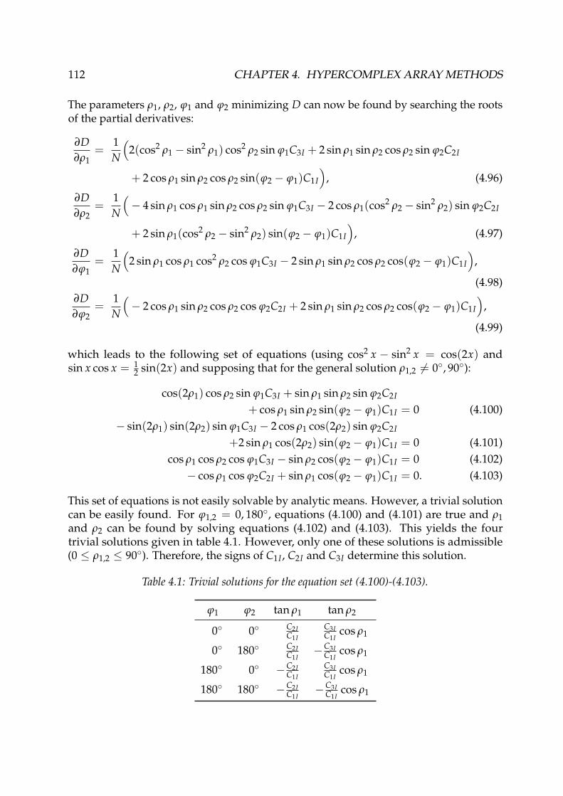
112 CHAPTER 4. HYPERCOMPLEX ARRAY METHODS

The parameters ρ1, ρ2, ϕ1 and ϕ2 minimizing D can now be found by searching the rootsof the partial derivatives:

∂D∂ρ1

=1N

(2(cos2 ρ1 − sin2 ρ1) cos2 ρ2 sin ϕ1C3I + 2 sin ρ1 sin ρ2 cos ρ2 sin ϕ2C2I

+ 2 cos ρ1 sin ρ2 cos ρ2 sin(ϕ2 − ϕ1)C1I

), (4.96)

∂D∂ρ2

=1N

(− 4 sin ρ1 cos ρ1 sin ρ2 cos ρ2 sin ϕ1C3I − 2 cos ρ1(cos2 ρ2 − sin2 ρ2) sin ϕ2C2I

+ 2 sin ρ1(cos2 ρ2 − sin2 ρ2) sin(ϕ2 − ϕ1)C1I

), (4.97)

∂D∂ϕ1

=1N

(2 sin ρ1 cos ρ1 cos2 ρ2 cos ϕ1C3I − 2 sin ρ1 sin ρ2 cos ρ2 cos(ϕ2 − ϕ1)C1I

),

(4.98)∂D∂ϕ2

=1N

(− 2 cos ρ1 sin ρ2 cos ρ2 cos ϕ2C2I + 2 sin ρ1 sin ρ2 cos ρ2 cos(ϕ2 − ϕ1)C1I

),

(4.99)

which leads to the following set of equations (using cos2 x − sin2 x = cos(2x) andsin x cos x = 1

2 sin(2x) and supposing that for the general solution ρ1,2 6= 0◦, 90◦):

cos(2ρ1) cos ρ2 sin ϕ1C3I + sin ρ1 sin ρ2 sin ϕ2C2I

+ cos ρ1 sin ρ2 sin(ϕ2 − ϕ1)C1I = 0 (4.100)− sin(2ρ1) sin(2ρ2) sin ϕ1C3I − 2 cos ρ1 cos(2ρ2) sin ϕ2C2I

+2 sin ρ1 cos(2ρ2) sin(ϕ2 − ϕ1)C1I = 0 (4.101)cos ρ1 cos ρ2 cos ϕ1C3I − sin ρ2 cos(ϕ2 − ϕ1)C1I = 0 (4.102)− cos ρ1 cos ϕ2C2I + sin ρ1 cos(ϕ2 − ϕ1)C1I = 0. (4.103)

This set of equations is not easily solvable by analytic means. However, a trivial solutioncan be easily found. For ϕ1,2 = 0, 180◦, equations (4.100) and (4.101) are true and ρ1and ρ2 can be found by solving equations (4.102) and (4.103). This yields the fourtrivial solutions given in table 4.1. However, only one of these solutions is admissible(0 ≤ ρ1,2 ≤ 90◦). Therefore, the signs of C1I , C2I and C3I determine this solution.

Table 4.1: Trivial solutions for the equation set (4.100)-(4.103).

ϕ1 ϕ2 tan ρ1 tan ρ2

0◦ 0◦ C2IC1I

C3IC1I

cos ρ1

0◦ 180◦ C2IC1I

−C3IC1I

cos ρ1

180◦ 0◦ −C2IC1I

C3IC1I

cos ρ1

180◦ 180◦ −C2IC1I

−C3IC1I

cos ρ1

4.5. BIQUATERNION-MUSIC 113

Nevertheless, biquaternion-MUSIC is intended to retrieve any polarization parametersof seismic motion. Therefore, the solutions given in 4.1 are not acceptable because theyimpose phase differences of 0◦ or 180◦ between the different components. Other solutionsof the equations (4.100)-(4.103) cannot be retrieved by analytic means. A grid searchwould be necessary for that purpose. However, a two-dimensional grid search for ρ1 andϕ2 is sufficient. Equation (4.103) then yields

ϕ1 = ϕ2 − arccos(

C2I cos ϕ2

C1I tan ρ1

), (4.104)

which is only valid if∣∣∣C2I cos ϕ2

C1I tan ρ1

∣∣∣ < 1, i.e.

ρ1 > arctan∣∣∣∣C2I

C1Icos ϕ2

∣∣∣∣ . (4.105)

Therefore, the grid search in ρ1 can be limited to the interval [arctan∣∣∣C2I

C1Icos ϕ2

∣∣∣ , 90◦],whereas the search for ϕ2 stretches the interval [0, 360◦[. Equation (4.104) has two solu-tions in the intervall [0◦, 360◦]. According to equation (4.102), ρ2 can then be determinedby

ρ2 = arctan(

C3I sin ρ1 cos ϕ1

C2I cos ϕ2

). (4.106)

As 0 ≤ ρ2 ≤ 90◦, C3I sin ρ1 cos ϕ1C2I cos ϕ2

has to be positive. The grid search of all admissiblesolutions yields the set (ρ1, ρ2, ϕ1, ϕ2) which minimizes equation (4.95).

4.5.2.1 Case of identical signals for all three components

A special case is given if the signals for the three components are identical(~X1( f ) = ~X2( f ) = ~X2( f )

). In this case, the three components of the correct steering

vector (equation (4.84)) should be equal, i.e.

cos ρ1 cos ρ2 = sin ρ1 cos ρ2 exp(iϕ1) = sin ρ2 exp(iϕ2), (4.107)

which is equivalent to

ρ1 = 45◦, (4.108)

ρ2 = arcsin(

1√3

), (4.109)

ϕ1 = 0◦, (4.110)ϕ2 = 0◦. (4.111)

Calculating the covariance matrix of the data vector ~Xbiq( f ) = ~X1( f ) · (i+ j+ k) gives

Sbiq = ~X†biq

~Xbiq

= ~X†1~X1 · (−i− j− k) · (i+ j+ k)

= 3~X†1~X1. (4.112)

114 CHAPTER 4. HYPERCOMPLEX ARRAY METHODS

Therefore, only the scalar part of the covariance matrix is non-zero and C1 = C2 = C3 = 0.Consequently, equation (4.95) simplifies to

D =C0

N(4.113)

and is independent of ρ1, ρ2, ϕ1 and ϕ2. Although this very simple special case is unreal-istic for real data measurements, the method should be able to resolve the polarizationparameters.

4.5.2.2 Case of identical signals for two components

If the signals for two components are identical, two polarization values are alreadyknown in theory. In the following, we will focus on the case ~X1( f ) = ~X2( f ), whichwould be described by ρ1 = 45◦ and ϕ1 = 0◦. In this case, the data vector is given by~Xbiq( f ) = ~X1( f ) (i+ j) + ~X2( f ) k, which gives the covariance matrix

Sbiq = ~X†biq

~Xbiq

=[~X†

1( f ) (−i− j)− ~X†3( f ) k

] [~X1( f ) (i+ j) + ~X3( f ) k

]= 2~X†

1( f )~X1( f ) + ~X†3( f )~X3( f ) + ~X†

1( f )~X3( f )(−i+ j) + ~X†3~X1( f )(i− j). (4.114)

Consequently, K(Sbiq) = 0 and C3 = 0.

Furthermore, as(~X†

1( f )~X3( f )(−i+ j))†

= ~X†3( f )~X1( f )(i− j), C1 = −C2.

Therefore, equation (4.95) can be written as

D =1N

[C0 + 2 sin ρ2 cos ρ2(cos ρ1 sin ϕ2 + sin ρ1 sin(ϕ2 − ϕ1))C1I ] . (4.115)

Setting the derivatives of D with respect to ρ1, ρ2, ϕ1 and ϕ2 to 0 then yields

∂D∂ρ1

=2C1I

Nsin ρ2 cos ρ2(− sin ρ1 sin ϕ2 + cos ρ1 sin(ϕ2 − ϕ1)) = 0, (4.116)

∂D∂ρ2

=2C1I

N(cos2 ρ2 − sin2 ρ2)(cos ρ1 sin ϕ2 + sin ρ1 sin(ϕ2 − ϕ1)) = 0, (4.117)

∂D∂ϕ1

= −2C1I

Nsin ρ2 cos ρ2 sin ρ1 cos(ϕ2 − ϕ1) = 0, (4.118)

∂D∂ϕ2

=2C1I

Nsin ρ2 cos ρ2(cos ρ1 cos ϕ2 + sin ρ1 cos(ϕ2 − ϕ1)) = 0. (4.119)

For the general solution where no components vanish, ρ1 and ρ2 are not allowed tobecome 0◦ or 90◦. Consequently, equations (4.116) - (4.119) are simplified to

− sin ρ1 sin ϕ2 + cos ρ1 sin(ϕ2 − ϕ1) = 0, (4.120)

(cos2 ρ2 − sin2 ρ2)(cos ρ1 sin ϕ2 + sin ρ1 sin(ϕ2 − ϕ1)) = 0, (4.121)cos(ϕ2 − ϕ1) = 0, (4.122)

cos ρ1 cos ϕ2 + sin ρ1 cos(ϕ2 − ϕ1) = 0. (4.123)

4.5. BIQUATERNION-MUSIC 115

Inserting equation (4.122) in equation (4.123) gives

cos ϕ2 = 0, (4.124)

and therefore ϕ2 = 90◦ or 270◦. Then, equation (4.122) yields ϕ1 = 0◦ or 180◦. However,for ϕ1 = 180◦, equation (4.120) has no solution for 0◦ < ρ1 < 90◦. Therefore, ϕ1 = 0◦.Inserting either value of ϕ2 in equation (4.120) gives tan ρ1 = 1 and therefore ρ1 = 45◦.Using the obtained values, equation (4.121) can only be solved if tan ρ2 = 1 and thereforeρ2 = 45◦. Inserting the obtained values in the formula for D given in equation (4.115)yields D = 1

N

(C0 +

√2 C1I

)for ϕ2 = 90◦ and D = 1

N

(C0 −

√2 C1I

)for ϕ2 = 270◦.

The sign of C1I decides whether ϕ2 = 90◦ or 270◦ corresponds to the minimum of D.In the case where the signal of two components is identical, the polarization betweenthese two components is well retrieved (i.e. ρ1 = 45◦ and ϕ1 = 0◦). However, thepolarization of the third component of the signal is always found to be ρ2 = 45◦ andϕ2 = 90◦ or 270◦ and therefore, the correct polarization is not retrievable in general.

4.5.2.3 Case of two-dimensional signals

The motion of Rayleigh waves is confined to a plane built by the vertical and radialcomponents, Love waves are confined to the transverse component. Therefore, for apure wave of one of both types, at least one component vanishes. Only in the presence ofadditional noise or both wave types in the same time, all three components are non-zero.Therefore, it is interesting to see how biquaternion-MUSIC is performing in these cases.In the following, it is supposed that the wave vector~k has already been determinedbefore searching for the polarization parameters.If one of the three components vanishes, the biquaternion data vector ~Xbiq( f ) givenin equation (4.83) will only have two non-zero quaternion parts and consequently,the biquaternion covariance matrix Sbiq given by equation (4.85) has only two non-vanishing parts: The scalar part and the part for which the data vector vanishes (i.e. ifI(~Xbiq( f )) = ~0, then J(Sbiq) = 0 and K(Sbiq) = 0). Consequently, the same propertyis valid for the eigenvectors of Sbiq and subsequently for C defined by equation (4.91),because the other components i and j cannot be generated by any product of a scalarpart and k. Therefore, two of the three components C1, C2 and C3 vanish.We will only show the case of a vanishing third component of ~Xbiq( f ), i.e. ~X3( f ) = ~0.Then, C1 = C2 = 0 and equation (4.95) simplifies to

D =1N

(C0 + 2 sin ρ1 cos ρ1 cos2 ρ2 sin ϕ1C3I

). (4.125)

116 CHAPTER 4. HYPERCOMPLEX ARRAY METHODS

The four derivatives of D with respect to ρ1, ρ2, ϕ1 and ϕ2 can then be set to 0, whichyields

∂D∂ρ1

=2N

(cos2 ρ1 − sin2 ρ1) cos2 ρ2 sin ϕ1C3I = 0, (4.126)

∂D∂ρ2

= − 2N

sin ρ1 cos ρ1 sin ρ2 cos ρ2 sin ϕ1C3I = 0, (4.127)

∂D∂ϕ1

=2N

sin ρ1 cos ρ1 cos2 ρ2 cos ϕ1C3I = 0, (4.128)

∂D∂ϕ2

= 0. (4.129)

The only parameter in equations (4.126) - (4.129) which depends on the measurements isC3I . Furthermore, this term is cancelled out. Therefore, the solutions of these equationsare independent of the measurements. In fact, equations (4.126) - (4.129) are solved byρ2 = π/2 and arbitrary values for the other parameters. Then, D = C0

N is constant andit is impossible to determine the polarization of the signal. In fact, the steering vectorgiven by equation (4.84) tries to bring the different components of the signal to equalamplitude and phase. In the case of a vanishing component, this is only possible if thesteering vector vanishes the other two components, which is achieved here by cos ρ2 = 0.If the first or second component of the signal vanishes, the reasoning is analog and willnot be shown here. It results that biquaternion-MUSIC is unable to retrieve the polariza-tion for signals with a vanishing component. Nevertheless, if a component vanishes, thepolarization relationship of the remaining two components can be very well retrieved us-ing quaternion-MUSIC. As Rayleigh waves are limited to two components, it is thus notnecessary to use biquaternion-MUSIC for their analysis. However, biquaternion-MUSICmight help in analyzing any complicated three-dimensional signal.

4.6. MUSIQUE 117

4.6 MUSIQUE

As shown above, the biquaternion-MUSIC approach does not work in certain specialcases (e.g. two-dimensional signal, identical signals for two or three components). Fur-thermore, the polarization of a pure seismic wave is always confined to two componentsmaximum. Therefore, the quaternion-MUSIC approach is sufficient to characterize thepolarization parameters of an incident wave. Consequently, the MUSIQUE algorithmconsists in a combination of the "classical" MUSIC and the quaternion-MUSIC algorithms.Figure 4.1 gives an overview of the method’s principle. The recordings of a seismic arrayconsisting of N sensors are cut into signal blocks of length T = nP/ f0, where nP indicatesthe number of periods in the signal and f0 is the frequency of interest. The data of asignal block are then given (in the time domain) by three data matrices xi ∈ RN×NT ,where i ∈ {1,2,3} stands for the vertical, eastern and northern components, respectively.NT is the number of data points in the signal block (NT = T/dt, dt indicating the timesampling of the signals). In order to better suppress wave contributions of differentfrequencies, the signals xi are prefiltered around f0 with a bandwidth of d f , but theactual MUSIC processing is narrow-band.

4.6.1 Estimation of the wave vector by MUSIC

A Fourier transform of xi yields the respective data matrices Xi ∈ CN×NS in the frequencydomain. As we are interested in the signal at a given frequency f0, we are interested inthe signal vectors ~X( f0) ∈ CN. According to equation (3.13), the covariance matrix atfrequency f0 is built for each component by

Si = E(~Xi( f0)~X†

i ( f0))

=f0+∆

∑f = f0−∆

~Xi( f )~X†i ( f ). (4.130)

Here, the expectation value is realized by summation over a small number of frequenciesaround f0. The width of ∆ depends on the frequency resolution of the Fourier transform.To ensure good results, it is sufficient to sum over five frequency values. Seismic signalscan occur on a single component or on all components together, depending on the motion.The motion of Love waves, for example, is confined to the horizontal components. Ifwe are only interested in Rayleigh waves, we could use the vertical component only.However, at the peak frequency of the ellipticity, the vertical Rayleigh wave motionvanishes. In order to correctly analyze the wave field, no component has to be omitted.Therefore, the MUSIQUE code is based on a covariance matrix which is simply built byadding the matrices of the single components:

S =3

∑i=1

Si. (4.131)

The "classical" MUSIC code described in 3.4 is applied to the covariance matrix defined inequation (4.131). The eigenvalues and eigenvectors of S are calculated and the noise sub-space is constructed. Then, the wave vector~k which maximizing the MUSIC functionalgiven in equation (3.21) is searched for.

118 CHAPTER 4. HYPERCOMPLEX ARRAY METHODS

(a)

0 1 2 3

N

E

Z

Time [s]

Sensor

(b)

0 1 2 3

N

E

Z

Time [s]Sensor

(c) (d)

0 1 2 3

T

R

Z

Time [s]Sensor

(e) (f)

Figure 4.1: Graphic outline of the MUSIQUE method: The original three-component signal (a)of all stations of an array of seismic sensors is (b) prefiltered and cut into signal blocks of someperiods of lenght. (c) A grid-search yields the wave vector (given by slowness and azimuth) whichmaximizes the "classical" MUSIC functional P given by equation (3.21). (d) By projecting theeastern and northern components of the signal in the azimuth and its orthogonal direction, theradial and transverse component signals are generated. Based on an energy criterium, the waveis identified either as a Love wave or as a possible Rayleigh wave. In the second case, (e) thepolarization parameters ρ and ϕ are found, using the vertical and radial signals, by maximizingthe quaternion-MUSIC functional Pq = 1/D, which is equivalent to (f) the minimization of D.Actually, ρ and ϕ can be calculated analytically and no grid search is necessary. The identificationof the wave type (retrograde or prograde Rayleigh wave) is based on the value of ϕ.

4.6. MUSIQUE 119

The wave vector~k, i.e. azimuth and slowness corresponding to the predominant wavesource are identifiedVI. The signals xi are then projected in the direction of the identifiedwave vector~k (with azimuth ϑ). Therefor, the vertical component x1 is left unchangedand the eastern component x2 and northern component x3 are transformed in the radialand transverse components by:

xradial = − sin ϑ · x2 − cos ϑ · x3

xtransverse = cos ϑ · x2 − sin ϑ · x3.

The energies of the different components are calculated by

Evertical =f0+∆

∑f = f0−∆

~X†1( f ) ~X1( f )

Eeast =f0+∆

∑f = f0−∆

~X†2( f ) ~X2( f )

Enorth =f0+∆

∑f = f0−∆

~X†3( f ) ~X3( f )

Eradial = sin2 ϑ · Eeast + cos2 ϑ · Enorth

Etransverse = cos2 ϑ · Eeast + sin2 ϑ · Enorth.

If the predominant wave is a Love wave, the transverse energy will dominate over thevertical and radial energies. On the other hand, if a Rayleigh wave is predominant,the transverse energy will be smaller than both other energies. It should be noted that,depending on the ellipticity at the frequency f0, either the vertical or the radial componentcan vanish although a Rayleigh wave is predominant. Therefore, the transverse energyis always compared to the sum of radial and vertical energies.In the MUSIQUE code, if Etransverse > Evertical + Eradial, the wave is identified as Lovewave and the processing stops here. In the contrary case, the predominant wave ispresumed to be a Rayleigh wave and its polarization parameters are estimated byapplying quaternion-MUSIC.

VIIn principle, MUSIC can identify multiple sources, i.e. correctly identify azimuths and slownesses ifmore than one source exist. However, the MUSIQUE code is principally built to retrieve the polarizationparameters of Rayleigh waves, which are estimated in the further processing. This processing does,indeed, not work for more than one incident wave, because the signal is projected in the azimuth directionidentified in the first step. This means that only the dominant arrival of each time window is analyzed.

120 CHAPTER 4. HYPERCOMPLEX ARRAY METHODS

4.6.2 Estimation of the polarization parameters by quaternion-MUSICThe Fourier transform of the radial and vertical data matrices xradial and x1 yields thematrices Xradial ∈ CN×NS and Xvertical = X1. Using these matrices, the quaternion-valuedsignal vector (equation (4.59)) is constructed as

~XMUSIQUE( f ) = <(~Xvertical( f )) + i · <(~Xradial( f )) + j=(~Xvertical( f )) + k · =(~Xradial( f )).(4.132)

In analogy to equation (4.131), the covariance matrix SMUSIQUE is built by

SMUSIQUE =f0+∆

∑f = f0−∆

~XMUSIQUE( f ) ~X†MUSIQUE( f ). (4.133)

As described in 4.4, the eigenvalues and eigenvectors of SMUSIQUE are calculated and thenoise subspace is constructed. Because the wave vector~k has already been determinedby the classical version of MUSIC, the polarization parameters ρ and ϕ which describethe relation between both components of the motion, are obtained by equations (4.80)and (4.82) which emerge from the analytic calculation presented in 4.4.2.

The particle motion of Rayleigh waves can be retrograde or prograde. In theory, ret-rograde motion corresponds to a phase difference ϕ = 90◦ and prograde motion toϕ = 270◦. We allow the phase differences to deviate 45◦ from these "perfect" phasedifferences, and identify waves with 45◦ < ϕ < 135◦ as retrograde Rayleigh waves andwaves with 225◦ < ϕ < 315◦ as prograde ones. For other values of ϕ, the wave is leftunclassified.

4.6. MUSIQUE 121

4.6.3 Assembling the resultsThe MUSIQUE code retrieves for every signal block:

• azimuth ϑ

• slowness s

• amplitude parameter ρ (for Rayleigh waves)

• phase difference ϕ (for Rayleigh waves)

• type of wave (Love wave, retrograde/prograde Rayleigh wave)

Thus, by analyzing a large number of signal blocks at different frequencies, the wave fieldcan be characterized. We denote by s( f ,m) the slowness of the mth block at frequencyf, by ρ( f ,m) the amplitude parameter, Evertical( f ,m), Eradial( f ,m) and Etransverse( f ,m) theenergies of the three components and by l( f ,m), rretro( f ,m) and rpro( f ,m) parameterswhich are 1 if the signal in the respective block was identified as Love wave, retrogradeor prograde Rayleigh wave, respectively, and 0 everywhere else. NB( f ) indicates thenumber of signal blocks analyzed at frequency f . Then, the dispersion curves areobtained by averaging over the different analyzed signal blocks in the following way:

sLove( f ) =∑

NB( f )m=1 l( f ,m) Etransverse( f ,m) s( f ,m)

∑NB( f )m=1 l( f ,m) Etransverse( f ,m)

, (4.134)

sRayleigh,retro( f ) =∑

NB( f )m=1 rretro( f ,m) [Evertical( f ,m) + Eradial( f ,m)] s( f ,m)

∑NB( f )m=1 rretro( f ,m) [Evertical( f ,m) + Eradial( f ,m)]

, (4.135)

sRayleigh,pro( f ) =∑

NB( f )m=1 rpro( f ,m) [Evertical( f ,m) + Eradial( f ,m)] s( f ,m)

∑NB( f )m=1 rpro( f ,m) [Evertical( f ,m) + Eradial( f ,m)]

. (4.136)

In a similar way, the Rayleigh wave ellipticity curves are obtained by:

εretro( f ) =∑

NB( f )m=1 rretro( f ,m)

√Evertical( f ,m) + Eradial( f ,m) sin(ρ( f ,m))

∑NB( f )m=1 rretro( f ,m)

√Evertical( f ,m) + Eradial( f ,m) cos(ρ( f ,m))

, (4.137)

εpro( f ) =∑

NB( f )m=1 rpro( f ,m)

√Evertical( f ,m) + Eradial( f ,m) sin(ρ( f ,m))

∑NB( f )m=1 rpro( f ,m)

√Evertical( f ,m) + Eradial( f ,m) cos(ρ( f ,m))

. (4.138)

However, misidentified signal blocks can introduce a large bias in the respective averagedispersion or ellipticity estimations. Therefore, in real data applications, it is preferableto plot a histogram of all identified signal blocks before finally determining the respectivecurves.

122 CHAPTER 4. HYPERCOMPLEX ARRAY METHODS

4.7 Conclusion

Two advanced versions of the MUSIC algorithm have been presented, which can beused to retrieve the polarization parameters of seismic waves. The quaternion-MUSICapproach is capable of retrieving the polarization relationship for two-component seis-mic signals. The biquaternion-MUSIC approach can retrieve the polarization of three-component signals. At first, this method appears rather appealing. However, for a lot ofspecial cases, this algorithm fails. Certainly, none of these special cases will ever occurfor real data measurements. Nevertheless, it is difficult to assume that the algorithmyields correct results in the general case if it fails for simple special cases. Furthermore,as seismic waves are always confined to a maximum of two directions of polarization,the quaternion-MUSIC approach is sufficient to investigate these waves. This is whatthe MUSIQUE technique does. By identifying the azimuth and velocity (or slowness,respectively) of the wave with "classical" MUSIC first, it is possible to separate the radialand transverse components of the signal. Then, the polarization parameters between thevertical and the radial component can be estimated by using the quaternion-MUSIC ap-proach. In contrast to other established array methods, MUSIQUE allows the distinctionbetween retrograde and prograde Rayleigh wave motion.

MUSIQUE will be tested on synthetic seismic signals in chapter 5 and applied to realseismological data in chapter 8. Furthermore, a comparison between DELFI, RayDec andMUSIQUE was presented at the European Signal Processing Conference (EUSIPCO) 2009in Glasgow, UK. The associated paper [Hobiger et al., 2009b] can be found in appendixA.

Chapter 5

Tests on synthetic data

In this chapter, the three methods DELFI, RayDec and MUSIQUE which were presentedin previous chapters (DELFI in 2.3, RayDec in 2.4 and MUSIQUE in 4.6) are tested onsynthetic seismic data. A first test investigates the behavior of the methods under theinfluence of additional white noise. In further tests, the methods are tested on signalsof increasing complexity, starting from single source signals and ending with ambientseismic vibration simulations with a random source distribution.

Dans ce chapitre, les trois nouvelles méthodes DELFI, RayDec et MUSIQUE présentées dans leschapitres précédents (DELFI en 2.3, RayDec en 2.4 et MUSIQUE en 4.6), seront testées sur desdonnées sismiques synthétiques. Un premier test examinera le comportement des différentesméthodes sous l’influence d’une addition de bruit blanc aux signaux. Dans les tests suivants, lesméthodes seront étudiées en les appliquant à des signaux de complexité croissante, commençantpar des signaux émanant d’une seule source jusqu’à des simulations de bruit sismique ambiantavec une distribution aléatoire de sources.

123

124 CHAPTER 5. TESTS ON SYNTHETIC DATA

5.1 Introduction

This thesis work includes three new method developments, which have been presentedabove (DELFI in section 2.3, RayDec in section 2.4 and MUSIQUE in section 4.6). DELFIand RayDec only estimate ellipticity, MUSIQUE estimates the azimuth, slowness ofseismic waves as well as the ellipticity parameter and phase difference between boththe vertical and radial component for Rayleigh waves. In this chapter, the respectiveestimations of these methods will be tested on synthetic seismic data of increasing com-plexity. The first test (section 5.2) investigates how the methods behave if white noise isadded to a perfect cosine signal. The white noise has a theoretical constant ellipticity of√

2 because the energies of the three different components are equal. This test includestwo different signal sets, one with an ellipticity of 5 and the other with an ellipticity of 0.3.

The next test (section 5.3) is based on a purely theoretical signal which is generated on thebasis of a dispersion curve and an ellipticity curve. The summed energy of the verticaland horizontal components of the signal is kept constant, whereas the relative energydistribution is fixed by the ellipticity curve. The propagation of waves originating ina distance of 20 km is modeled corresponding to the dispersion curve. In this way, thewave parameters are completely controlled. The ellipticity estimations of DELFI andRayDec are compared to the H/V results and the MUSIQUE results for three arrays ofdifferent sizes are compared to the results for analyzing all stations together.

In section 5.4, ambient seismic vibrations are simulated. For two different distributionsof the seismic sources (in the first one, all sources are located in a specific direction, inthe second one, the source distribution is random), DELFI, RayDec and MUSIQUE aretested and the results compared.

5.2. INFLUENCE OF THE SIGNAL-TO-NOISE RATIO 125

5.2 Influence of the signal-to-noise ratio

5.2.1 Signal generationThis section investigates the influence of the signal-to-noise ratio (SNR) on the results forthe three newly developed methods. The test is based on a synthetic, monochromaticretrograde Rayleigh wave signal. This signal consists of a pure cosine of a frequency of0.77 Hz, propagating across an array of seismic sensors with a slowness of 0.59 s/km(i.e. a velocity of 1.69 km/s) under an azimuth of 30◦. The seismic array consists of eightstations, regularly spaced on a ring of 1.5 km radius surrounding a central station. Itslayout is displayed in figure 5.1.

−2000 −1000 0 1000 2000

−1000

0

1000

Distance [m]

Dis

tanc

e [m

]

Figure 5.1: Layout of the seismic array used for the tests.

Two different signals have been generated, the first with an ellipticity of 5, the secondwith an ellipticity of 0.3.White noise of variable energy content was added to the signal. The signal-to-noise ratiois defined as

SNR[dB] = 10 log10

(Esignal

Enoise

), (5.1)

where the energies Esignal and Enoise are calculated on signals which are prefilteredaround the analyzed frequency. Notably, these energies are calculated for a given three-component signal consisting of N data points as

E =N

∑i=1

(v2(ti) + e2(ti) + n2(ti)

), (5.2)

where v(ti), e(ti) and n(ti) indicate the signals on the vertical, eastern and northerncomponent, respectively.

126 CHAPTER 5. TESTS ON SYNTHETIC DATA

For tests involving the MUSIQUE technique, a single window of 5 cycles length (i.e.6.5 s long) was analyzed, adding random noise with an energy corresponding to theSNR value and repeating the test 1 000 times. For tests of DELFI and RayDec, a signalof 5 minutes length was generated, random noise with an energy corresponding to theSNR value was added and a total of 1 000 different realizations of this performed perSNR. Signal-to-noise ratios between 0 dB and 20 dB have been investigated. Accordingto equation (5.1), a SNR of 0 dB corresponds to a signal where the energies of the signalpart and the noise part are equal. For a SNR of 10 dB, the signal energy is ten times thenoise energy. In figure 5.2, example signals for SNR values of 0 dB, 10 dB and 20 dB areshown for both used signals, i.e. with theoretical ellipticities of 5 and 0.3.

(a)

0 30 60 90 120

−2

−1

0

1

2

Am

plitu

de

Time [s]

Vertical component

0 dB10 dB20 dB

0 30 60 90 120

−2

−1

0

1

2

Am

plitu

de

Time [s]

Eastern component

0 dB10 dB20 dB

0 30 60 90 120

−2

−1

0

1

2

Am

plitu

de

Time [s]

Northern component

0 dB10 dB20 dB

(b)

0 30 60 90 120−2

−1

0

1

2

Am

plitu

de

Time [s]

Vertical component

0 dB

10 dB

20 dB

0 30 60 90 120−2

−1.5

−1

−0.5

0

0.5

1

1.5

2

Am

plitu

de

Time [s]

Eastern component

0 dB10 dB20 dB

0 30 60 90 120−2

−1.5

−1

−0.5

0

0.5

1

1.5

2

Am

plitu

de

Time [s]

Northern component

0 dB10 dB20 dB

Figure 5.2: Example signals of the vertical (left), eastern (center) and northern (right) componentsfor different signal-to-noise ratios for signals with a theoretical ellipticity of (a) 5 and (b) 0.3.

5.2. INFLUENCE OF THE SIGNAL-TO-NOISE RATIO 127

5.2.2 Analysis resultsIn figure 5.3, the results for the first test (with a theoretical ellipticity of 5) are shown. Themean azimuth, slowness, phase difference and ellipticity values obtained by averagingthe results of analyzing 1 000 signal realizations at each SNR value using MUSIQUEare shown and compared to the signal parameters. The wave vector, i.e. azimuth andslowness, is obtained using the "classical" MUSIC method (see 3.4). It can be seen thatfor signal-to-noise ratios above 10, the correct azimuth and slowness values are retrievedfor every signal realization (figures 5.3 (a) and (b)). The average value of the azimuthestimation is rather stable and deviates significantly from the true azimuth for SNR’sbelow 5. For SNR = 0, the mean azimuth estimation equals 43◦. In addition, the errorbars of the mean azimuth estimation are negligible for SNR’s above 10 and increasestrongly for SNR’s below 7. The mean slowness estimation is correct for SNR’s above 7.Below this value, the slowness is systematically overestimated. In the same range, theerror bars of this estimation increase strongly.The polarization parameters, i.e. the phase difference ϕ between vertical and horizon-tal signal (figure 5.3 (c)) and the ellipticity (figure 5.3 (d)), are determined using thecalculation which is based on the previous azimuth and slowness estimation and waspresented in 4.4.2. Therefore, it cannot be expected that the polarization parameters arewell estimated if the wave vector is misestimated. Nevertheless, for the phase differenceϕ, the mean estimation is in very good agreement with the theoretical value for all SNRratios. However, for low SNR values the standard deviation increases. The averageellipticity estimation is in good agreement with the actual value for SNR’s above 8. Belowthis value, the ellipticity is underestimated a lot. Nevertheless, over the whole SNR range,the error bars are rather large. Figures 5.3 (e) and (f) have been calculated in the sameway as (c) and (d), but fixing the correct azimuth and slowness values before estimatingthe wave polarization. This eliminates the effects of the wrong slowness estimation atlow SNR’s. As a result, the average phase difference still fits the actual one, but the errorbars are reduced. Now, the average estimation and the true curve of the ellipticity are inagreement for SNR’s above 5 and the misestimation at low SNR values is reduced, withreduced error bars.

128 CHAPTER 5. TESTS ON SYNTHETIC DATA

(a)

0 5 10 15 200

90

180

270

360

SNR [dB]

Azi

mut

h [°

]

(b)

0 5 10 15 200

1

2

3

4

SNR [dB]

Slo

wne

ss [s

/km

]

(c)

0 5 10 15 200

90

180

270

360

SNR [dB]

ϕ[◦

]

(d)

0 5 10 15 200

2

4

6

8

SNR [dB]

Elli

ptic

ity

(e)

0 5 10 15 200

90

180

270

360

SNR [dB]

ϕ[◦

]

(f)

0 5 10 15 200

2

4

6

8

SNR [dB]

Elli

ptic

ity

Figure 5.3: MUSIQUE results for adding white noise to a pure Rayleigh wave signal with anellipticity of 5. 1 000 realizations per value of the signal-to-noise ratio (SNR) have been analyzed:average (a) azimuth, (b) slowness, (c) phase difference between the vertical and horizontalcomponents and (d) ellipticity estimations. (e) Phase difference and (f) ellipticity for correctlyestimated azimuth and slowness values. The solid line marks the average value, the shaded areasindicate the standard deviation. The dotted lines represent the actual values of the respectiveparameters for the signal.

5.2. INFLUENCE OF THE SIGNAL-TO-NOISE RATIO 129

(a)

0 5 10 15 200

2

4

6

8

SNR [dB]

Elli

ptic

ity

DELFI

(b)

0 5 10 15 200

2

4

6

8

SNR [dB]

Elli

ptic

ity

RayDec

Figure 5.4: Results for adding white noise to a pure Rayleigh wave signal with an ellipticity of 5.Analyzing 1 000 realizations per SNR value using (a) DELFI, (b) RayDec. The solid line marksthe average value, the shaded areas indicate the standard deviation. The dotted lines represent theactual values of the respective parameters for the signal.

The performances of DELFI and RayDec analyzing the same 1 000 realizations of the-oretical signals per SNR are displayed in figures 5.4 (a) and (b), respectively. For bothmethods, the average ellipticity estimation decreases monotonically with decreasingSNR, without significant increase of the standard deviation. It is rather surprising thata quite small amount of noise largely influences the ellipticity estimation of these twomethods. A possible explanation is that both methods exploit the time correlation be-tween the vertical and horizontal components of a Rayleigh wave. With a theoreticalellipticity of 5, the combined energy of the horizontal components is 25 times larger thanthe energy of the vertical component of the signal part. As the added noise has the sameenergy on all three components, the noise added on the vertical component has a muchlarger influence than the SNR ratio would suggestI. Therefore, the added noise puts arelatively large amount of energy on the vertical component. Consequently, the ellipticityis underestimated. As RayDec uses the vertical component as a trigger, the method israther vulnerable to added noise on the vertical componentII.

IFor example, a SNR of 10 corresponds to Esignal = 10 Enoise. The noise energy is equally distributedon the three components (Enoise,vert = Enoise,north = Enoise,east = 1

3 Enoise), whereas with an ellipticityof 5 the signal energy is mostly concentrated on the horizontal components (Esignal,north + Esignal,east =25 Esignal,vert = 25

26 Esignal . Consequently, the signal and noise contributions to the vertical component arealmost equal (Esignal,vert = 30

26 Enoise,vert).IIThe signal is stacked for every zero-crossing of the vertical component. All stacked signals are finally

summed. If the noise on the vertical component is strong, it will also shift a large part of the zero-crossingsand induce instabilities in the final ellipticity estimation.

130 CHAPTER 5. TESTS ON SYNTHETIC DATA

The results for the second test with a theoretical ellipticity of 0.3 are shown in figure 5.5.As in the previous test, the results are obtained by averaging 1 000 signal realizations. Forthe azimuth and slowness values (figures 5.5 (a) and (b)), the results are almost identicalto the previous case, with a correct azimuth and slowness retrieval for every run forSNR’s above 10. For an SNR of 0, the mean azimuth is estimated as 42◦. Nevertheless,the slowness overestimation at low SNR values is slightly larger than in the previouscase.The phase difference ϕ estimation is equivalent to the previous case, i.e. the averageestimated value fits the actual value and the error bars increase monotonically with de-creasing SNR. However, the ellipticity estimation is much more robust against additionalnoise than in the previous case. The average value fits the actual value even for lowSNR’s and the standard deviation rises less with a decrease of the SNR.For DELFI (figure 5.5 (e)), at high SNR’s the actual ellipticity value is well retrieved andincreases monotonically with a decreasing SNR. RayDec (figure 5.5 (f)) exhibits the samebehavior, but the absolute misestimation and the error bars are smaller. In this case withan ellipticity value of 0.3, the signal energy on the vertical component is 11 times thecombined signal energy on the horizontal components. Therefore, the added noise actsvery little on the vertical component and the RayDec estimation is more robust than inthe previous case for a high ellipticity.

5.2.3 Discussion of the results

The results suggest that the azimuth estimation is much more stable against noise con-tributions than the slowness estimation. This can be seen in both cases, where even fora SNR of 0, the azimuth estimation error does not exceed 13◦, whereas the slowness isoverestimated to about three times its actual value.A part of the ellipticity misestimation for MUSIQUE in the first test can be explained bythe slowness misestimation, but even for a correct slowness estimation, the ellipticityis systematically underestimated for high noise levels. The added noise has the sameenergy level on all three components, which corresponds to a theoretical H/V ratio of√

2 of this partIII. Therefore, adding noise on data with an ellipticity exceeding√

2 tendsto underestimate the actual ellipticity value, while the effect for adding noise on datawith lower ellipticity is the opposite. This can be seen in the results for all three methods.Furthermore, it seams that the ellipticity estimation using MUSIQUE is more robustagainst noise than using DELFI or RayDec. This might be linked to the fact thatMUSIQUE uses an array of sensors. As the noise recorded on the different sensorsis uncorrelated, an array can more efficiently suppress noise contributions.

IIIIf the energies of all three components are equal, the H/V ratio is calculated as

HV

=

√Enorth + Eeast

Evert=√

2.

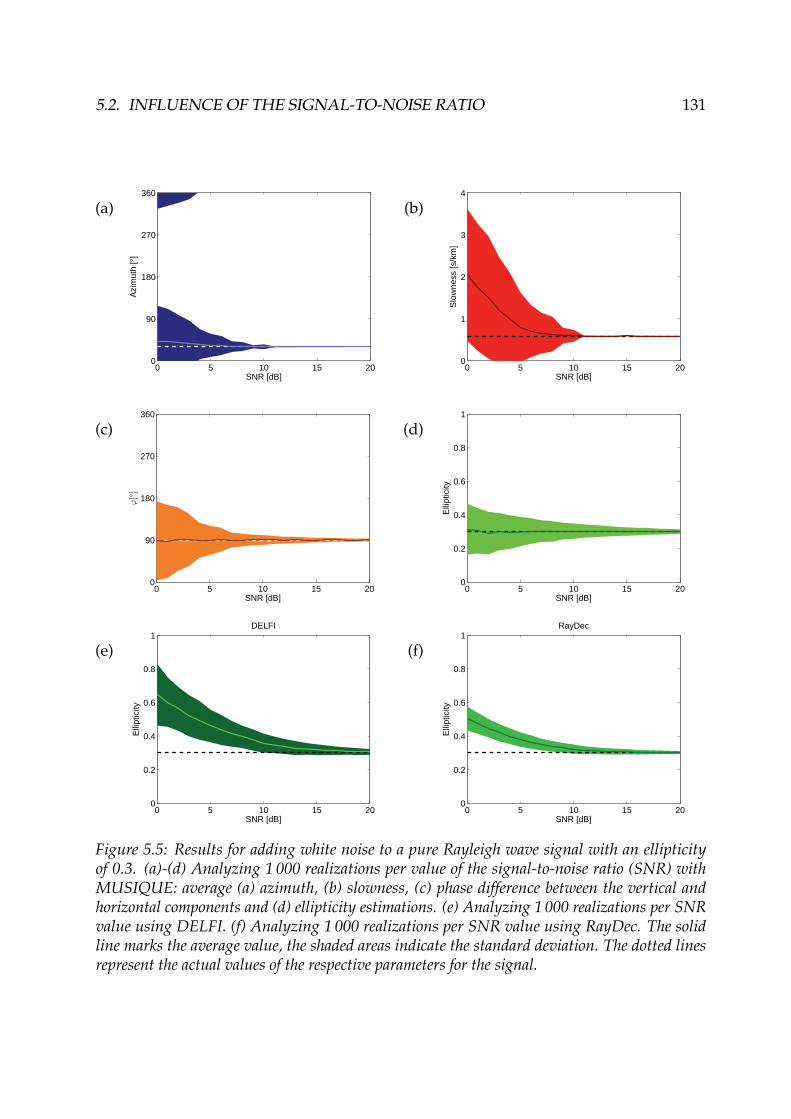
5.2. INFLUENCE OF THE SIGNAL-TO-NOISE RATIO 131

(a)

0 5 10 15 200

90

180

270

360

SNR [dB]

Azi

mut

h [°

]

(b)

0 5 10 15 200

1

2

3

4

SNR [dB]

Slo

wne

ss [s

/km

]

(c)

0 5 10 15 200

90

180

270

360

SNR [dB]

ϕ[◦

]

(d)

0 5 10 15 200

0.2

0.4

0.6

0.8

1

SNR [dB]

Elli

ptic

ity

(e)

0 5 10 15 200

0.2

0.4

0.6

0.8

1

SNR [dB]

Elli

ptic

ity

DELFI

(f)

0 5 10 15 200

0.2

0.4

0.6

0.8

1

SNR [dB]

Elli

ptic

ity

RayDec

Figure 5.5: Results for adding white noise to a pure Rayleigh wave signal with an ellipticityof 0.3. (a)-(d) Analyzing 1 000 realizations per value of the signal-to-noise ratio (SNR) withMUSIQUE: average (a) azimuth, (b) slowness, (c) phase difference between the vertical andhorizontal components and (d) ellipticity estimations. (e) Analyzing 1 000 realizations per SNRvalue using DELFI. (f) Analyzing 1 000 realizations per SNR value using RayDec. The solidline marks the average value, the shaded areas indicate the standard deviation. The dotted linesrepresent the actual values of the respective parameters for the signal.

132 CHAPTER 5. TESTS ON SYNTHETIC DATA

5.3 Tests on a theoretical dispersive signal

5.3.1 Signal generationThis test is based on a completely theoretical signal. The reason for this is to test themethods on a signal where we control all properties. The dispersion curves sRayleigh( f )and sLove( f ) and ellipticity curve ε( f ) shown in figures 5.6 (a) and (b) are used for thegeneration of the signal. For the stations of the seismic array (see figure 5.6 (c) for thearray layout), plane Rayleigh and Love waves originating in a distance of dS = 20 kmfrom the array center with azimuth ϑ = 30◦ are calculated as described in the following.The array is composed of three rings of eight sensors each at radii of 60, 300 and 1 500meters, respectively, and a central station. The total energy at each frequency is keptconstant by setting the sum of vertical energy Ev( f ) and radial energy Er( f ) to 1. On the

other hand, vertical and radial motions are linked through the ellipticity ε( f ) =√

Er( f )Ev( f ) .

This fixes the values of Ev( f ) and Er( f ) to:

Ev( f ) =1

ε2( f ) + 1, (5.3)

Er( f ) =ε2( f )

ε2( f ) + 1. (5.4)

In a first simulation, only Rayleigh waves are accounted for. In a second test, Lovewaves are added. Thus, in the first simulation Et( f ) = 0 and in the second simulation,Et( f ) = 1, where Et( f ) is the transverse energy.The signals at the source are stationary cosine signals. An additional parameter m( f )parameterizes the retrograde or prograde sense of motion of the Rayleigh wave: atfrequencies below the ellipticity peak and beyond the trough, m = 1; between the peakand trough frequencies, m = −1. The vertical, radial and transverse signals at the sourceare defined by:

vS(t) =f2∫

f1

√Ev( f ) · sin(2π f t)d f , (5.5)

rS(t) =f2∫

f1

√Er( f ) · sin(2π f t + m( f )π/2)d f , (5.6)

tS(t) =f2∫

f1

√Et( f ) · sin(2π f t)d f . (5.7)

If the position of the ith sensor is given by ~pi and the position of the source by ~pS, then

their distance along the ray path is given by di = |~pS| −~pT

i ~pS|~pS|

= dS −~pT

i ~pSdS

.

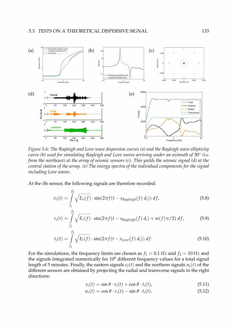
5.3. TESTS ON A THEORETICAL DISPERSIVE SIGNAL 133

(a)

0.1 1 10

1

10

Frequency [Hz]

Slo

wne

ss [s

/km

]

Retrograde Rayleigh wavePrograde Rayleigh waveLove wave

(b)

0.1 1 10

0.1

1

10

100

Frequency [Hz]

Elli

ptic

ity

Retrograde Rayleigh wavePrograde Rayleigh wave

(c)

−2000 −1000 0 1000 2000

−1000

0

1000

Distance [m]

Dis

tanc

e [m

]

(d) (e)

0.1 1 100

2000

4000

6000

Frequency [Hz]E

nerg

y

Total

Vertical

Radial

Transverse

Figure 5.6: The Rayleigh and Love wave dispersion curves (a) and the Rayleigh wave ellipticitycurve (b) used for simulating Rayleigh and Love waves arriving under an azimuth of 30◦ (i.e.from the northeast) at the array of seismic sensors (c). This yields the seismic signal (d) at thecentral station of the array. (e) The energy spectra of the individual components for the signalincluding Love waves.

At the ith sensor, the following signals are therefore recorded:

vi(t) =f2∫

f1

√Ev( f ) · sin(2π f (t− sRayleigh( f ) di)) d f , (5.8)

ri(t) =f2∫

f1

√Er( f ) · sin(2π f (t− sRayleigh( f ) di) + m( f )π/2) d f , (5.9)

ti(t) =f2∫

f1

√Et( f ) · sin(2π f (t− sLove( f ) di)) d f . (5.10)

For the simulations, the frequency limits are chosen as f1 = 0.1 Hz and f2 = 10 Hz andthe signals integrated numerically for 106 different frequency values for a total signallength of 5 minutes. Finally, the eastern signals ei(t) and the northern signals ni(t) of thedifferent sensors are obtained by projecting the radial and transverse signals in the rightdirections:

ei(t) = sin ϑ · ri(t) + cos ϑ · ti(t), (5.11)ni(t) = cos ϑ · ri(t)− sin ϑ · ti(t). (5.12)

134 CHAPTER 5. TESTS ON SYNTHETIC DATA

Although the signal is composed of cosine waves, the signal content is not the same ateach time sample. In fact, a real Dirac signal is composed of an infinite number of cosinewaves which interfere constructively at one point in time. This is the case of the presentedsignal at the source, although the energy content is not the same at all frequencies. Forthe stations of the array, the dispersion of the waves leads to a divergence of the differentfrequency contents. In this way, the produced signal is not too far away from a realseismic signal produced by a single hammer blow, for example. This can be seen infigure 5.6 (d) where the signal simulated for the central station of the array includingLove waves is shown. In the case without Love waves, the vertical and radial signals arethe same, but the transverse signal vanishes. The associated spectra of the individualcomponents of this signal are shown in figure 5.6 (e).

5.3.2 Analysis results

5.3.2.1 Single-sensor ellipticity estimation

The results for applying the three single-sensor methods H/V, DELFI and RayDec to thetheoretical signals are shown in figure 5.7.

H/VIn the case without Love waves, the H/V curve (figure 5.7 (a)) corresponds to themodel’s ellipticity curve. This is a direct consequence of the signal generation. In thecase including Love waves, however, the H/V curve overestimates ellipticity becauseadditional energy is present on the transverse component (figure 5.7 (b)).

DELFIThe DELFI results for the central station of the array are shown in figures 5.7 (c) and (d)for different filtering bandwidths. In the processing, signal blocks of one period lengthwere analysed. As can be seen in figure 5.7 (c) for the signal without Love waves, theretrieved ellipticity curve is very close to the model curve over the whole frequencyrange, and the curve is best fitted for the smallest filtering bandwidth, i.e. d f = 0.1 f .In figure 5.7 (d), the results for the signal including Love waves are shown. At lowfrequencies, the ellipticity is clearly overestimated, but at frequencies above the peakfrequency, the agreement is very satisfactory, again with the best results for the smallestfilter bandwidth, d f = 0.1 f . This can be explained because at low frequencies, Love andRayleigh waves have approximately the same slownesses. Therefore, the contributions ofboth wave types arrive at almost the same time at the array and overlap. Consequently,DELFI’s estimation of the ellipticity is biased at these frequencies. At higher frequencies,the dispersion curves of Rayleigh and Love waves are different and therefore, the wavepackets arrive at different times. DELFI succeeds in discriminating the Love waves inthis case. Consequently, the ellipticity estimation is very close to the real curve here.However, it should be noted that DELFI cannot retrieve the correct ellipticity neither atthe ellipticity peak nor at the trough. At these points, either the vertical or the radialcomponent of the Rayleigh wave vanishes and therefore the ellipse degenerates into alinear motion. Thus, the fitting of an ellipse at these points must fail.

5.3. TESTS ON A THEORETICAL DISPERSIVE SIGNAL 135

(a)

1 10 1

0.1

1

10

100

Frequency [Hz]

Elli

ptic

ity

modelH/V (b)

1 10 1

0.1

1

10

100

Frequency [Hz]

Elli

ptic

ity

modelH/V

(c)

0.1 1 10

0.1

1

10

100

Frequency [Hz]

Elli

ptic

ity

modelDELFI, df = 0.1 fDELFI, df = 0.15 fDELFI, df = 0.2 f

(d)

0.1 1 10

0.1

1

10

100

Frequency [Hz]

Elli

ptic

ity

modelDELFI, df = 0.1 fDELFI, df = 0.15 fDELFI, df = 0.2 f

(e)

0.1 1 10

0.1

1

10

100

Frequency [Hz]

Elli

ptic

ity

modelRayDec, df = 0.1 fRayDec, df = 0.15 fRayDec, df = 0.2 f

(f)

0.1 1 10

0.1

1

10

100

Frequency [Hz]

Elli

ptic

ity

modelRayDec, df = 0.1 fRayDec, df = 0.15 fRayDec, df = 0.2 f

Figure 5.7: (a) and (b) H/V curves obtained for the synthetic signal without Love waves andincluding Love waves, respectively. (c) and (d) Curves obtained by DELFI for the respectivecases with and without Love waves, both for different values of the frequency filter bandwidthd f . (e) and (f) RayDec curves for the respective cases, for different values of the frequency filterbandwidth d f .

136 CHAPTER 5. TESTS ON SYNTHETIC DATA

RayDecFigures 5.7 (e) and (f) show the results for applying RayDec to the signals at the centralstation of the array, again for different filter bandwidths. The number of cycles used inthe code was set to 10. In figure 5.7 (e), no Love waves are present and the ellipticityestimation is in very good agreement for all filter bandwidths. At the peak and troughfrequencies, the results are better for sharper filters. When adding Love waves (see figure5.7 (f)), the results of the smallest filter bandwidth (d f = 0.1 f ) are less stable than forthe larger bandwidths. At frequencies below the peak, the ellipticity is overestimated.At the right flank of the peak, the measurement is in very good agreement with themodel. Above the trough frequency, some instabilities in the ellipticity estimation can beseen. Again, these results can be explained by the close velocities of the Rayleigh andLove waves at low frequencies. In addition to the simultaneous arrival of both surfacewave types at the array stations, the Love and Rayleigh waves of the simulation havea constant phase difference throughout the simulated signal. Therefore, the horizontalpart of the Rayleigh wave is overestimated.RayDec exploits the well-defined phase relationship between vertical and horizontalsignal to discriminate against other wave types. Therefore, at points where one of bothRayleigh components vanishes, the ellipticity estimation will always be biased if otherwave types are present. This explains why the estimated ellipticity curves cannot fit thereal model data at the ellipticity’s peak and trough.

ComparisonIn the case of a theoretical signal without Love waves, all three methods succeed inretrieving the correct ellipticity curve. In the presence of Love waves, however, H/Voverestimates the ellipticity curve. The left flank is overestimated by DELFI and RayDec,probably because Rayleigh and Love waves are present at the same time for thesefrequencies. DELFI retrieves the right flank of the peak and the part beyond the trough,but fails at the peak and trough frequencies. RayDec retrieves the correct right flank anddeviates above the trough frequency. All methods succeed in finding the frequency ofthe ellipticity peak.

5.3.2.2 MUSIQUE

The signals have been analyzed by MUSIQUE both processing all stations at the sametime and considering the different rings separately. For every analyzed frequency, theprocessing described in 4.6 was performed, i.e. the signal was cut into blocks of 5 periodslength and for each block the azimuth and slowness values were estimated. Love andRayleigh waves have been detected and the polarization parameters of the Rayleighwaves estimated. The dispersion curves shown in the following correspond to the meanvalue for the respective wave type at the analyzed frequency.Figure 5.8 displays the results for analyzing all stations simultaneously for the caseswithout Love waves (figures 5.8 (a) and (b)) and including Love waves (figures 5.8 (c)and (d)). In both cases, the dispersion curves are well retrieved. Some prograde Ray-leigh waves are found at higher frequencies, although the motion should be retrograde.Around 4 Hz, the array is losing its resolution and aliasing effects occur.

5.3. TESTS ON A THEORETICAL DISPERSIVE SIGNAL 137

At frequencies where the Rayleigh wave motion changes from prograde to retrogradeand vice versa, both curves continue across that frequency and deviate there. The corre-sponding ellipticity values are very well retrieved with some data points of misestimatedpolarization. In the case including Love waves, (c), both Love and Rayleigh wave disper-sion curves are well estimated up to the resolution limit of the array (around 4 Hz). Theellipticity curve in (d) is well retrieved up to this frequency.In theory, the prefiltering in the MUSIQUE algorithm should be redundant, as the codeitself takes the signal at some frequencies only and the filtering should not bias the re-spective information. However, if strong sources at certain frequencies are present in thesignal, they can "leak" into neighboring frequency ranges and alter the results. Figures5.8 (e) and (f) are equivalent to (c) and (d), but the prefiltering process in the MUSIQUEcode has been omitted. Evidently, the results are less clear with misestimated Loveand prograde Rayleigh wave slowness values, especially at low frequencies. At higherfrequencies, all dispersion curves are not as clearly retrieved as with the prefiltering. Onthe ellipticity curve, the effect is even more obvious as the retrograde and prograde wavemotions are not well distinguished any more and the ellipticity values are misestimated.As these effects are already visible for a completely theoretical signal, they will be evenmore pronounced for real seismic signals, which justifies prefiltering the signals.The data processing time increases with the number of seismic sensorsIV. In fact, it cannotbe expected that the array stations on the 1500-meter ring contribute to the analysis ofhigh-frequency signals. Indeed, including too many sensors which do not contributeto the analysis can even worsen the results. Due to aliasing effects, both outer ringscould not correctly estimate the properties of the waves for frequencies above 3 Hz in thisexample. Therefore, the estimation at higher frequencies is based on the smallest ringonly and could be accelerated by omitting the larger rings. Surely, the presented arraywith an outer ring radius 25 times larger than the inner ring radius is a rather extremeexample, but if the measurements are supposed to cover a large frequency range, suchan array size is necessary.In figure 5.9, the dispersion and ellipticity curves for analyzing the stations of one ring(plus the central station) only are shown, both without Love waves ((a) - (f)) and includingLove waves ((g) - (l)). In the case without Love waves, dispersion and ellipticity curves arecorrectly estimated in every case. In the case including Love waves, the dispersion curvesare well retrieved in the respective resolution limits of the single arrays. The ellipticitycurves are better estimated than in the case of analyzing all stations at the same time.Notably the smallest array (figures 5.9 (i) and (l)) resolves better for frequencies around4 Hz compared to the case including all stations in figures 5.8 (c) and (d). Therefore, bycombining the results of the different subarrays, a better result can be achieved than forusing all stations simultaneously. Furthermore, the computation time decreases.

IVNot only more data have to be processed, but in the algorithm, the eigenvalues and eigenvectors of anN × N data matrix have to be determined (where N indicates the number of sensors).

138 CHAPTER 5. TESTS ON SYNTHETIC DATA

(a)

0.1 1 10

1

10

Frequency [Hz]

Slo

wne

ss [s

/km

]

Retrograde Rayleigh wavePrograde Rayleigh wave (b)

0.1 1 10

0.1

1

10

100

Frequency [Hz]

Elli

ptic

ity

Retrograde Rayleigh wavesPrograde Rayleigh waves

(c)

0.1 1 10

1

10

Frequency [Hz]

Slo

wne

ss [s

/km

]

Retrograde Rayleigh wavesPrograde Rayleigh wavesLove waves

(d)

0.1 1 10

0.1

1

10

100

Frequency [Hz]

Elli

ptic

ity

Retrograde Rayleigh wavesPrograde Rayleigh waves

(e)

0.1 1 10

1

10

Frequency [Hz]

Slo

wne

ss [s

/km

]

Retrograde Rayleigh wavesPrograde Rayleigh wavesLove waves

(f)

0.1 1 10

0.1

1

10

100

Frequency [Hz]

Elli

ptic

ity

Retrograde Rayleigh wavesPrograde Rayleigh waves

Figure 5.8: Results of applying MUSIQUE to the theoretical signals: (a) dispersion curve, (b)ellipticity curve for the case without Love waves; (c) dispersion curve, (d) ellipticity curve for thecase with Love waves. (e) dispersion and (f) ellipticity curve including Love waves, but withoutprefiltering the signal. The dashed and dotted lines indicate roughly the resolution limits of thearray, and correspond to s = 1

2dmax f , s = 1dmax f , s = 1

2dmin f and s = 1dmin f .

5.3. TESTS ON A THEORETICAL DISPERSIVE SIGNAL 139

(a)

0.1 1 10

1

10

Frequency [Hz]

Slo

wne

ss [s

/km

]

Retrograde Rayleigh wavesPrograde Rayleigh waves (b)

0.1 1 10

1

10

Frequency [Hz]

Slo

wne

ss [s

/km

]

Retrograde Rayleigh wavesPrograde Rayleigh waves (c)

0.1 1 10

1

10

Frequency [Hz]

Slo

wne

ss [s

/km

]

Retrograde Rayleigh wavesPrograde Rayleigh waves

(d)

0.1 1 10

0.1

1

10

100

Frequency [Hz]

Elli

ptic

ity

Retrograde Rayleigh wavesPrograde Rayleigh waves

(e)

0.1 1 10

0.1

1

10

100

Frequency [Hz]

Elli

ptic

ity

Retrograde Rayleigh wavesPrograde Rayleigh waves

(f)

0.1 1 10

0.1

1

10

100

Frequency [Hz]

Elli

ptic

ity

Retrograde Rayleigh wavesPrograde Rayleigh waves

(g)

0.1 1 10

1

10

Frequency [Hz]

Slo

wne

ss [s

/km

]

Retrograde Rayleigh wavesPrograde Rayleigh wavesLove waves

(h)

0.1 1 10

1

10

Frequency [Hz]

Slo

wne

ss [s

/km

]

Retrograde Rayleigh wavesPrograde Rayleigh wavesLove waves

(i)

0.1 1 10

1

10

Frequency [Hz]

Slo

wne

ss [s

/km

]

Retrograde Rayleigh wavesPrograde Rayleigh wavesLove waves

(j)

0.1 1 10

0.1

1

10

100

Frequency [Hz]

Elli

ptic

ity

Retrograde Rayleigh wavesPrograde Rayleigh waves

(k)

0.1 1 10

0.1

1

10

100

Frequency [Hz]

Elli

ptic

ity

Retrograde Rayleigh wavesPrograde Rayleigh waves

(l)

0.1 1 10

0.1

1

10

100

Frequency [Hz]

Elli

ptic

ity

Retrograde Rayleigh wavesPrograde Rayleigh waves

Figure 5.9: Results of applying MUSIQUE to the theoretical signals, using only one ring ofsensors plus the central station: dispersion and ellipticity curves for the largest ring without Lovewaves (a, d) and with Love waves (g, j); The corresponding curves for the medium ring without(b, e) and with Love waves (h, k) and for the smallest ring without (c, f) and with Love waves (i,l). The dashed and dotted lines indicate roughly the resolution limits of the array, and correspondto s = 1

2dmax f , s = 1dmax f , s = 1

2dmin f and s = 1dmin f .

140 CHAPTER 5. TESTS ON SYNTHETIC DATA

5.4 Tests on simulated seismic signals

5.4.1 Signal generationThe following tests are based on a more realistic simulation of real seismic noise sig-nals (body and surface waves), i.e. signals which are combinations of the signals ofmany sources [Bonnefoy-Claudet et al., 2006]. The signals were simulated using thewavenumber-based technique of Hisada [1994, 1995]. For given source signals andpositions, the propagation of seismic waves and their recordings for a given array ofseismic sensors are simulated, using the soil structure given in table 5.1. The dispersionand ellipticity curves corresponding to this model are shown in figures 5.10 (a) and (b).The array is composed of three concentric rings of 8 stations each with radii of 50, 200and 400 meters, respectively, and a central station.A first test simulates seismic waves arriving from a principal source region. The noisesource positions are located inside a circle of 100 meter radius. The center of this circlelies in a distance of 1 250 meters from the array center under an azimuth of 30◦ (see figure5.10 (c) for the source locations with respect to the array of seismic sensors).In a second test, the seismic sources are distributed randomly around the array (seefigure 5.10 (d)). The minimum distance of a noise source to the array center is 900 meters,in order to keep a minimum distance of 500 meters between any source and any sensor.In both tests, the source time functions are Dirac peaks. At each source point, a seismicsource was simulated once during the total simulation duration of 17.8 minutes. Inboth tests, a total of 320 sources have been used and two simulations per test have beenperformed. The first one uses only vertically oriented source forces. Thus, no Love wavesare generated. The second one also includes horizontally oriented forces and thereforeLove waves.

Table 5.1: Parameters of the model used for the simulation using Hisada’s code: Thickness ranged, pressure wave velocity VP, shear wave velocity VS and density ρ of the layers, and the qualityfactors QP and QS with respect to P- and S-waves.

d[m] VP[m/s] VS[m/s] ρ[kg/m3] QP QS

0−20 1 500 400 2 000 200 10020−∞ 5 600 3 200 2 000 200 100

5.4. TESTS ON SIMULATED SEISMIC SIGNALS 141

(a)

1 100.1

1

Frequency [Hz]

Slo

wne

ss [s

/km

]

Retrograde Rayleigh wavePrograde Rayleigh waveLove wave

(b)

1 100.01

0.1

1

10

100

Frequency [Hz]

Elli

ptic

ity

Retrograde Rayleigh wavePrograde Rayleigh wave

(c)

−500 0 500 1000−500

0

500

1000

Distance [m]

Dis

tanc

e [m

]

Sensors

Noisesources

(d)

−2000 −1000 0 1000 2000−2000

−1000

0

1000

2000

Distance [m]

Dis

tanc

e [m

]

Sensors

Noisesources

Figure 5.10: (a) The Rayleigh and Love wave dispersion curves and (b) the Rayleigh waveellipticity curve corresponding to the model given in table 5.1 which was used for the simulationof a transient seismic signal. (c) and (d) Positions of the sources and the array sensors forseismic noise simulations with multiple sources. (a) The sources are located on a circle of 100radius, which is located 1 250 m from the array center under an azimuth of 30◦. (b) The sourcedistribution is random, but no source is closer than 500 m to a seismic sensor.

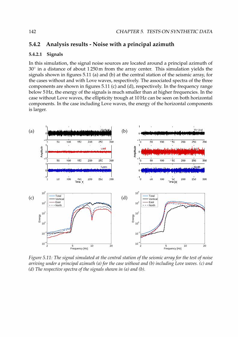
142 CHAPTER 5. TESTS ON SYNTHETIC DATA

5.4.2 Analysis results - Noise with a principal azimuth

5.4.2.1 Signals

In this simulation, the signal noise sources are located around a principal azimuth of30◦ in a distance of about 1 250 m from the array center. This simulation yields thesignals shown in figures 5.11 (a) and (b) at the central station of the seismic array, forthe cases without and with Love waves, respectively. The associated spectra of the threecomponents are shown in figures 5.11 (c) and (d), respectively. In the frequency rangebelow 5 Hz, the energy of the signals is much smaller than at higher frequencies. In thecase without Love waves, the ellipticity trough at 10 Hz can be seen on both horizontalcomponents. In the case including Love waves, the energy of the horizontal componentsis larger.

(a) (b)

(c)

2 5 10 2010

−4

10−2

100

102

104

106

Frequency [Hz]

Ene

rgy

TotalVerticalEastNorth

(d)

2 5 10 2010

−4

10−2

100

102

104

106

Frequency [Hz]

Ene

rgy

TotalVerticalEastNorth

Figure 5.11: The signal simulated at the central station of the seismic array for the test of noisearriving under a principal azimuth (a) for the case without and (b) including Love waves. (c) and(d) The respective spectra of the signals shown in (a) and (b).

5.4. TESTS ON SIMULATED SEISMIC SIGNALS 143

5.4.2.2 Single-sensor ellipticity estimation

In figure 5.12, the results of applying the three single-sensor methods H/V, DELFI andRayDec to the signals simulated for the central station are shown. The left column showsthe results for the signal withouth Love waves and the right column including Lovewaves.

H/VThe H/V curve for the case without Love waves (figure 5.12 (a)) fits the theoreticalellipticity curve perfectly above 5 Hz and is in good agreement at the left ellipticity flank.For the case including Love waves (figure 5.12 (b)), the H/V curve is in disagreementwith the ellipticity curve in any frequency range and largely overestimates particularlythe right flank.

DELFIThe DELFI results using a block size of one period and different values for the filterbandwidth d f are shown in figures 5.12 (c) and (d). The curves for both cases fit the rightflank of the ellipticity peak and for every value of the frequency bandwidth parameter.However, below the peak frequency and around the trough, the theoretical curve ispoorly fitted, especially in the case including Love waves.

RayDecThe results for applying RayDec to the same data are shown in figures 5.12 (e) and (f)for different filter bandwidths. The number of cycles used by RayDec was set to 10. Forthe case without Love waves (figure 5.12 (e)), the curves are in good agreement withthe right flank of the ellipticity peak. For the case including Love waves , the ellipticityvalues of the right flank are slightly overestimated (figure 5.12 (f)), the results for thelargest filter bandwidth still being the closest to the real curve. Below the peak frequency,the ellipticity curve is not fitted in both cases.

ComparisonThe results below the peak frequency can be explained by the fact that the energies of thenoise signals at low frequencies are very low on all components (see figures 5.11 (c) and(d)). Comparing the right flank of the ellipticity peak, in the case without Love waves, allmethods yield accurate results. In the case including Love waves, H/V does not fit theellipticity curve in a satisfactory way, while the results of DELFI and RayDec are muchcloser to the right flank of the true curve.

144 CHAPTER 5. TESTS ON SYNTHETIC DATA

(a)

1 10

0.1

1

10

100

Frequency [Hz]

Elli

ptic

ity

modelH/V (b)

1 10

0.1

1

10

100

Frequency [Hz]

Elli

ptic

ity

modelH/V

(c)

1 10

0.1

1

10

100

Frequency [Hz]

Elli

ptic

ity

modelDELFI, df = 0.1 fDELFI, df = 0.15 fDELFI, df = 0.2 f

(d)

1 10

0.1

1

10

100

Frequency [Hz]

Elli

ptic

ity

modelDELFI, df = 0.1 fDELFI, df = 0.15 fDELFI, df = 0.2 f

(e)

1 10

0.1

1

10

100

Frequency [Hz]

Elli

ptic

ity

modelRayDec, df = 0.1 fRayDec, df = 0.15 fRayDec, df = 0.2 f

(f)

1 10

0.1

1

10

100

Frequency [Hz]

Elli

ptic

ity

modelRayDec, df = 0.1 fRayDec, df = 0.15 fRayDec, df = 0.2 f

Figure 5.12: H/V curves for the signal simulated at the central array station with sources of aprincipal azimuth for (a) the case without Love waves and (b) with Love waves. The respectiveDELFI curves for different filter bandwidths d f (c) without and (d) with Love waves. (e) and (f)give the respective curves for RayDec, for different filter bandwidths.

5.4. TESTS ON SIMULATED SEISMIC SIGNALS 145

5.4.2.3 MUSIQUE

MUSIQUE has been applied to the simulations using 5 minutes of the signal for allstations of the array simulataneously. At each frequency, the analysis was performed onsignal blocks with lengths of three cycles.

Dispersion curvesThe resulting dispersion curves are shown in figure 5.13. The different figures show theslowness values for all time windows which have been identified as Love, retrogradeor prograde Rayleigh waves, respectively, and are coded as distribution densities. Thedarker colors indicate that more time windows have been identified around the respectivevalue.It is evident that in the case with exclusively vertical source polarizations, i.e. withoutLove waves (left column of figure 5.13), the Love wave dispersion curve cannot beretrieved (figure 5.13 (a)). Only a few signals have been misidentified as Love waves.However, the energy of the respective time windows represents only 0.1 % of the totalanalyzed energy. This energy corresponds to the total energy of the time windowsidentified as Love waves and is calculated over the complete analyzed frequency range.The time windows attributed to retrograde and prograde Rayleigh waves account for15.7 % and 54.9 % of the total analyzed energy, respectively, while the unclassified timewindows represent 29.3 %. In the structure model, retrograde Rayleigh waves occurbelow 5 Hz and above 10 Hz. In figure 5.13 (c), both branches are correctly identified.In figure 5.13 (e), the prograde Rayleigh wave dispersion curve is well found in itsrespective frequency range.In the case including Love waves (right column of figure 5.13), the Love wave dispersioncurve is overall retrieved (figure 5.13 (b)), but the Rayleigh wave dispersion curve isalso seen due to some misidentified Rayleigh waves. The retrograde Rayleigh wavedispersion curve is retrieved below 4 Hz, but at frequencies around 10 Hz, Love wavesare identified as Rayleigh waves (figure 5.13 (d)). The prograde dispersion curve iswell retrieved, but also a part of the Love waves is misidentified (figure 5.13 (d)). Theanalyzed time windows attributed to Love waves carry 59.3 % of the total analyzedenergy in this case, retrograde Rayleigh waves 7.6 %, prograde Rayleigh waves 16.3 %and 16.8 % are unclassified.In all figures, misestimated waves are present at high slowness values. Their linear shapein the log-log plot indicates that these are probably aliasing effects. Furthermore, someLove waves are misidentified as Rayleigh waves and vice versa. Therefore, an automaticidentification and averaging of the results does not yield reliable results.

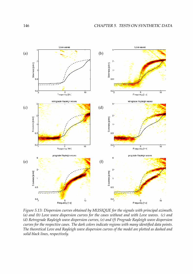
146 CHAPTER 5. TESTS ON SYNTHETIC DATA

(a) (b)

(c) (d)

(e) (f)

Figure 5.13: Dispersion curves obtained by MUSIQUE for the signals with principal azimuth.(a) and (b) Love wave dispersion curves for the cases without and with Love waves. (c) and(d) Retrograde Rayleigh wave dispersion curves, (e) and (f) Prograde Rayleigh wave dispersioncurves for the respective cases. The dark colors indicate regions with many identified data points.The theoretical Love and Rayleigh wave dispersion curves of the model are plotted as dashed andsolid black lines, respectively.

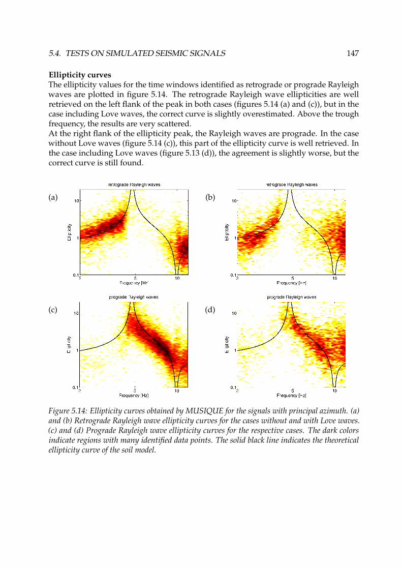
5.4. TESTS ON SIMULATED SEISMIC SIGNALS 147

Ellipticity curvesThe ellipticity values for the time windows identified as retrograde or prograde Rayleighwaves are plotted in figure 5.14. The retrograde Rayleigh wave ellipticities are wellretrieved on the left flank of the peak in both cases (figures 5.14 (a) and (c)), but in thecase including Love waves, the correct curve is slightly overestimated. Above the troughfrequency, the results are very scattered.At the right flank of the ellipticity peak, the Rayleigh waves are prograde. In the casewithout Love waves (figure 5.14 (c)), this part of the ellipticity curve is well retrieved. Inthe case including Love waves (figure 5.13 (d)), the agreement is slightly worse, but thecorrect curve is still found.

(a) (b)

(c) (d)

Figure 5.14: Ellipticity curves obtained by MUSIQUE for the signals with principal azimuth. (a)and (b) Retrograde Rayleigh wave ellipticity curves for the cases without and with Love waves.(c) and (d) Prograde Rayleigh wave ellipticity curves for the respective cases. The dark colorsindicate regions with many identified data points. The solid black line indicates the theoreticalellipticity curve of the soil model.

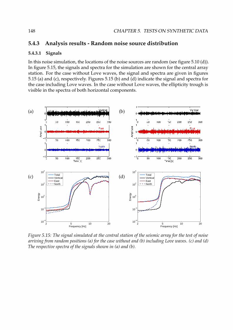
148 CHAPTER 5. TESTS ON SYNTHETIC DATA

5.4.3 Analysis results - Random noise source distribution

5.4.3.1 Signals

In this noise simulation, the locations of the noise sources are random (see figure 5.10 (d)).In figure 5.15, the signals and spectra for the simulation are shown for the central arraystation. For the case without Love waves, the signal and spectra are given in figures5.15 (a) and (c), respectively. Figures 5.15 (b) and (d) indicate the signal and spectra forthe case including Love waves. In the case without Love waves, the ellipticity trough isvisible in the spectra of both horizontal components.

(a) (b)

(c)

2 5 10 2010

−4

10−2

100

102

104

Frequency [Hz]

Ene

rgy

TotalVerticalEastNorth

(d)

2 5 10 2010

−4

10−2

100

102

104

Frequency [Hz]

Ene

rgy

TotalVerticalEastNorth

Figure 5.15: The signal simulated at the central station of the seismic array for the test of noisearriving from random positions (a) for the case without and (b) including Love waves. (c) and (d)The respective spectra of the signals shown in (a) and (b).

5.4. TESTS ON SIMULATED SEISMIC SIGNALS 149

5.4.3.2 Single-sensor ellipticity estimation

Figure 5.16 shows the results of applying the three single-sensor methods H/V, DELFIand RayDec to the signals simulated for the central station with a random source distri-bution.

H/VIn the case without Love waves (5.16 (a)), the H/V curve overestimates the actualellipticity curve over the whole frequency range (except for the peak), but is in acceptableagreement. For the case including Love waves (5.16 (b)), however, the overestimation isvery strong over the whole frequency range.

DELFIThe DELFI results using signal blocks of one period and different values for the filterbandwidth d f are shown in figures 5.16 (c) and (d). In the case without Love waves, thetheoretical ellipticity curve is underestimated. This underestimation is more pronouncedat the left flank of the peak, the right flank is actually well retrieved. For the caseincluding Love waves (5.16), DELFI overestimates both the left and the right flank ofthe peak. No significant differences between the curves corresponding to different filterbandwidths d f can be stated.

RayDecThe RayDec curves shown in figures 5.16 (e) and (f) have been obtained by setting thenumber of cycles used in the method to 10 and varying the filter bandwidth. For the casewithout Love waves (figure 5.16 (e)), RayDec fundamentally underestimates the actualellipticity curve over the whole frequency range and for all filter bandwidths d f . In thecase including Love waves (5.16 (f)), the RayDec curves are in very good agreementwith the theoretical ellipticity curve, especially at the left flank. For the right flank, thebest agreement with the measurements is obtained for setting d f = 0.15 f , but the othervalues also yield very good results. Around the trough frequency, however, the RayDeccurves do not follow the theoretical curve.

ComparisonAs a conclusion, it can be stated that, considering the right flank of the ellipticity peak,the best result in the case without Love waves is obtained by DELFI, whereas the bestresult including Love waves is obtained by RayDec. If Love waves are present, nomethod succeeds in resolving the trough of the curve. The bad results for frequenciesbelow the peak can be explained by the low energy content of the signal in this range.The underestimation of RayDec (and DELFI) of the right flank in the case without Lovewaves might be linked to some interaction between different wave types increasing thevertical signal or weakening the horizontal signals.The correct peak frequency (4.77 Hz) is hardly retrieved by any method. In the casewithout Love waves, H/V (4.98 Hz) and RayDec (4.86 Hz) overestimate the frequency,while DELFI (4.78 Hz) finds the correct value.

150 CHAPTER 5. TESTS ON SYNTHETIC DATA

In the case including Love waves, H/V (4.86 Hz) slightly overestimates, while DELFIand RayDec (both 4.64 Hz) underestimate the correct frequency.

(a)

1 10

0.1

1

10

100

Frequency [Hz]

Elli

ptic

ity

modelH/V (b)

1 10

0.1

1

10

100

Frequency [Hz]

Elli

ptic

ity

modelH/V

(c)

1 10

0.1

1

10

100

Frequency [Hz]

Elli

ptic

ity

modelDELFI, df = 0.1 fDELFI, df = 0.15 fDELFI, df = 0.2 f

(d)

1 10

0.1

1

10

100

Frequency [Hz]

Elli

ptic

ity

modelDELFI, df = 0.1 fDELFI, df = 0.15 fDELFI, df = 0.2 f

(e)

1 10

0.1

1

10

100

Frequency [Hz]

Elli

ptic

ity

modelRayDec, df = 0.1 fRayDec, df = 0.15 fRayDec, df = 0.2 f

(f)

1 10

0.1

1

10

100

Frequency [Hz]

Elli

ptic

ity

modelRayDec, df = 0.1 fRayDec, df = 0.15 fRayDec, df = 0.2 f

Figure 5.16: H/V curves for the signal simulated at the central array station for random noisesource distribution for (a) the case without Love waves and (b) with Love waves. The respectiveDELFI curves for different filter bandwidths d f (c) without and (d) with Love waves. (e) and (f)give the respective curves for RayDec, for different filter bandwidths.

5.4. TESTS ON SIMULATED SEISMIC SIGNALS 151

5.4.3.3 MUSIQUE

The data set generated by a random distribution of noise sources has been analyzed byMUSIQUE as well, using 5 minutes of the signal for all stations of the array simultane-ously. The length of the signal blocks was set to three cycles for the analysis.

Dispersion curvesThe resulting dispersion curves are shown in figure 5.17. The different figures show theslowness values for all time windows which have been identified as Love, retrogradeor prograde Rayleigh waves, respectively, and are coded as distribution densities. Thedarker colors indicate that more time windows have been identified at the respectivevalue.In the case without Love wave generation (left column of figure 5.17), some progradeRayleigh waves are misidentified as Love waves (figure 5.17 (a)), but their energy rep-resents only 0.5 % of the total analyzed energy. This energy corresponds to the totalenergy of the time windows identified as Love waves, covering the complete analyzedfrequency range. The time windows attributed to retrograde and prograde Rayleighwaves account for 20.7 % and 32.7 % of the total analyzed energy, respectively, while theunclassified time windows represent 46.1 %. According to the soil structure model, theRayleigh waves should be prograde in the frequency range between 5 and 10 Hz andretrograde below and above that frequency region. In figure 5.17 (c), the Rayleigh wavedispersion curve is well fitted in the regions corresponding to retrograde motion. Theprograde Rayleigh wave dispersion curve is well retrieved in its respective frequencyrange as well (5.17 (e)).In the case including Love waves (right column of figure 5.17), the Love wave dispersioncurve is very well retrieved in the whole frequency range (figure 5.17 (b)). The retrogradeRayleigh wave dispersion curve is retrieved in the frequency range below 5 Hz (figure5.17 (d)), but the high-frequency branch corresponds to misidentified Love waves. Theprograde Rayleigh wave dispersion curve, however, is well retrieved in its frequencyrange between 5 and 10 Hz (figure 5.17 (f)), but a second branch of misidentified Lovewaves is present in this case as well. In this case, time windows attributed to Lovewaves carry 27.0 % of the complete analyzed energy, retrograde Rayleigh waves 17.4 %,prograde Rayleigh waves 19.7 % and 35.9 % of the energy is unclassified.All figures exhibit aliasing artifacts, especially for high frequency and slowness values,but to a smaller extent at lower frequencies, too. These artifacts prevent automaticidentification and averaging algorithms of the results from being reliable.

152 CHAPTER 5. TESTS ON SYNTHETIC DATA

(a) (b)

(c) (d)

(e) (f)

Figure 5.17: Dispersion curves obtained by MUSIQUE for the signals with random noise sourcedistribution. (a) and (b) Love wave dispersion curves for the cases without and with Love waves.(c) and (d) Retrograde Rayleigh wave dispersion curves, (e) and (f) Prograde Rayleigh wavedispersion curves for the respective cases. The dark colors indicate regions with many identifieddata points. The theoretical Love and Rayleigh wave dispersion curves of the model are plotted asdashed and solid black lines, respectively.

5.4. TESTS ON SIMULATED SEISMIC SIGNALS 153

Ellipticity curvesIn figure 5.18, the ellipticity values for the time windows identified as retrograde orprograde Rayleigh waves are plotted. In the case without Love waves, the retrogradeRayleigh wave ellipticity is quite well retrieved at the left ellipticity peak (figure 5.18 (a)),but even in the case including Love waves, this part of the ellipticity curve is well fitted(figure 5.18 (b)).The prograde part, i.e. the right flank of the Rayleigh wave ellipticity peak, is wellretrieved in the case without Love wave generation (figure 5.18 (c)). In the case includingLove waves (figure 5.18 (d)), however, it is not retrieved at all.

(a) (b)

(c) (d)

Figure 5.18: Ellipticity curves obtained by MUSIQUE for the signals with random noise sourcedistribution. (a) and (b) Retrograde Rayleigh wave ellipticity curves for the cases without andwith Love waves. (c) and (d) Prograde Rayleigh wave ellipticity curves for the respective cases.The dark colors indicate regions with many identified data points. The solid black line indicatesthe theoretical ellipticity curve of the soil model.

154 CHAPTER 5. TESTS ON SYNTHETIC DATA

5.5 Conclusion

In this chapter, the performances of the newly developed methods DELFI, RayDec andMUSIQUE have been tested on synthetic data sets and compared to the results of theH/V method.

Test resultsThe first test investigated the robustness of the methods’ results against additional whitenoise. For MUSIQUE, the azimuth estimation is more robust than the slowness esti-mation. The misestimation of both influences the subsequent polarization parameterestimation. For this estimation, the phase difference parameter between the horizontaland vertical components is more robust than the ellipticity estimation. For DELFI andRayDec, adding white noise tends to underestimate ellipticity values above

√2 and

to overestimate lower ellipticity values. Compared to DELFI, RayDec is more robustagainst the addition of white noise.

The next tests compared the estimations of the different methods for signals of increasingcomplexity.For a simple theoretical signal, DELFI, RayDec and MUSIQUE retrieved the correctellipticity curve (or at least the right flank of the peak). H/V only retrieved the correctcurve in the case without Love waves. Furthermore, MUSIQUE correctly identifiesthe different wave types and discriminates between retrograde and prograde Rayleighwaves.For multiple signals with a principal direction of arrival, H/V only fits the ellipticitycurve if no Love waves are present, while RayDec and DELFI correctly estimate theright flank of the ellipticity peak, but not the rest of the curve. MUSIQUE identifies thedifferent wave types and estimates correct dispersion curves, as well as the ellipticitycurve.

The final test simulated real seismic noise with waves arriving from different azimuths.Of the single-sensor methods, only DELFI gives a correct ellipticity estimation of theright flank if no Love waves are present. In the general case with Love waves, the onlymethod to retrieve the correct right ellipticity flank is RayDec. In this case, MUSIQUEcorrectly identifies the different wave types and estimates the respective dispersioncurves. Although the right ellipticity peak is only retrieved if no Love waves are present,the distinction between prograde and retrograde Rayleigh waves helps in identifyingtheir respective parts of the dispersion curve.

5.5. CONCLUSION 155

Field of application of the different methodsAccording to their respective qualities, the different methods should be used in differentsituations. The mono-sensor methods RayDec and DELFI can be used to characterizeambient seismic vibrations. As RayDec is based on the statistics of summing a multitudeof signal blocks, it is especially suited for these investigations. The minimum requiredsignal length depends on the frequency range of interest. Nevertheless, as less as fiveminutes of signal can be sufficient for reliable resultsV. However, the method is notsuitable for signals of short duration, e.g. earthquake data. DELFI is less robust againstadditional Love wave contributions than RayDec and gives results which are similarto H/V for ambient seismic vibrations which are composed of both Rayleigh and Lovewaves with a random azimuth distribution. Therefore, the method should only be ap-plied to pure Rayleigh wave data if it is supposed to measure ellipticity. Nonetheless,by applying both RayDec and DELFI to the same measurements of ambient seismicvibrations, the composition of the seismic wave field, i.e. the relation between Love andRayleigh wave energy, can be estimated using a single seismic sensor.

As MUSIQUE uses array data, it can discriminate between retrograde and prograde Ray-leigh waves, which is not possible with single-sensor methods. Furthermore, it allows theestimation of azimuth and slowness, i.e. the wave vector, of incoming waves. The correctidentification between retrograde and prograde Rayleigh waves separates the Rayleighwave dispersion curve in two distinct branches. This distinction is not possible with otherestablished methods. However, for real ambient seismic vibration data, single-sensormethods should be preferred to estimate ellipticity. Although MUSIQUE can be appliedto long-duration recordings, it requires a lot of computation time, notably because of therepeated use of Fourier transforms and eigenvalue decompositions. Therefore, it is moreconvenient for short data sets, e.g. earthquake data which consist of transient seismicsignals.

The following part of this work will deal with the application of the developed methodsto real data measurements. Chapter 6 deals with the theoretical aspects of the inversionof ellipticity curves in order to find the local soil structure. The obtained results will thenbe applied to real seismic data measurements in chapter 7, where RayDec is used for theellipticity estimation. Finally, in chapter 8, real earthquake data measured in Californiawill be analyzed using MUSIQUE.

VThe necessary signal length depends on the frequency range of interest, five minutes are sufficient forfrequencies above about 0.3 Hz.

Part II

Application

Chapter 6

Inversion of ellipticity curves -Theoretical aspects

In previous chapters, methods to retrieve the ellipticity of Rayleigh waves have beenintroduced (DELFI in section 2.3, RayDec in section 2.4 and MUSIQUE in section 4.6)and tested (chapter 5). The ellipticity will now be used to retrieve the soil structure byinversion, using SPAC measurements (section 3.5) as additional information to constrainthe superficial structure. In this chapter, the fundamentals of the inversion of ellipticitycurves will be developed. The following text represents the article "Inversion of Rayleighwave ellipticity measurements, Part I: Theoretical aspects" by Hobiger, Cornou, Bard, LeBihan, and Wathelet, 2010a, which was submitted to Geophysical Journal International.

Dans les chapitres précédents, des méthodes pour déterminer l’ellipticité des ondes de Rayleighont été introduites (DELFI en 2.3, RayDec en 2.4 et MUSIQUE en 4.6) et testées (chapitre 5).Maintenant, l’ellipticité sera utilisée pour retrouver la structure du sol par inversion, contraignantla structure superficielle par des mesures SPAC (cf. 3.5) additionnelles. Dans le chapitre suivant,les aspects théoriques de l’inversion de courbes d’ellipticité seront développés. Le texte duchapitre correspond à l’article "Inversion of Rayleigh wave ellipticity measurements, Part I:Theoretical aspects" par Hobiger, Cornou, Bard, Le Bihan, and Wathelet, 2010a, qui a étésoumis à Geophysical Journal International.

159

160 CHAPTER 6. ELLIPTICITY INVERSION - THEORETICAL ASPECTS

6.1 Abstract

The knowledge of the local soil structure is important for the assessment of seismichazards. A widespread, but expensive and time-consuming technique to retrieve theparameters of the local underground is the drilling of boreholes. Furthermore, the shearwave velocity profile at a given location can be obtained by inversion of surface wavedispersion curves. In order to ensure a good resolution for both superficial and deeperlayers, the used dispersion curves need to cover a wide frequency range. This widefrequency range can be obtained using several arrays of seismic sensors or a single arraycomposed of a large number of sensors. Consequently, these measurements are time-consuming. A simpler alternative is provided by the use of the ellipticity of Rayleighwaves. The frequency dependence of the ellipticity is tightly linked to the shear wavevelocity profile. Furthermore, it can be measured using a single seismic sensor. As soilstructures which are obtained by scaling of a given model exhibit the same ellipticitycurve, an inversion of the ellipticity curve alone will always yield ambiguous results.Therefore, additional measurements which fix the shear wave velocity profile at somepoints have to be included in the inversion process. Small-scale spatial autocorrelationmeasurements or MASW measurements can provide the needed data. We will showwhich parts of the ellipticity curve have to be included in the inversion process to get areliable result and which parts can be omitted. Furthermore, the use of autocorrelation orhigh-frequency dispersion curves will be highlighted and the bias on the inversion resultswhich is produced by incorrect ellipticity curve measurements is shown. The rules forellipticity inversion resulting from these studies are applied to real data measurementsin an accompanying article.

6.2 Introduction

In order to assess the seismic hazard of a given site, the knowledge of the site conditionsis important. The local soil can be investigated by different means. For example, thedrilling of boreholes gives a good view of the ground structure, but is a time-consumingand expensive task. Refraction or reflection measurements using explosive sources aredifficult to be carried out in urban areas. On the contrary, active sources like sledgeham-mering can be used in urban areas, but generate waves only in a high frequency rangewhich does not penetrate the soil very deeply. Therefore, within agglomerations, therecording of seismic ambient vibrations is appropriate. Arrays of seismic sensors canbe easily deployed and dispersion curves of surface waves can be measured. Then, thelocal soil structure is obtained by inverting the dispersion curves. However, in orderto cover a broad frequency band, several seismic arrays have to be deployed [Watheletet al., 2008]. As a result, such measurements are time-consuming. In urban areas, theexisting infrastructure limits the possible deployment locations of the seismic sensors.Therefore, using a lower number of sensors is tempting.The ellipticity of Rayleigh waves, i.e. the ratio between the horizontal and the verticalmovement, strongly depends on the local soil structure and carries information on thecomplete sedimentary layers. The possibility of using ellipticity measurements to con-

6.2. INTRODUCTION 161

strain the soil structure was already shown by Boore and Toksöz [1969]. A widespreadtechnique for investigating the soil structure is the classical H/V technique [Nogoshiand Igarashi, 1971, Nakamura, 1989]. The H/V ratio simply indicates the spectral ratiobetween the horizontal and the vertical components. If the wave field was composedexclusively of single mode Rayleigh waves, the H/V ratio would indicate their ellipticity.In general, however, the seismic noise field is composed of various modes of Rayleighwaves, Love waves and body waves. The composition of the wave field depends onthe noise sources and the site structure [Bonnefoy-Claudet et al., 2008]. However, themeasurement of the ellipticity is not trivial in seismic noise recordings, since Love andbody waves contribute to the wave field as well [Köhler et al., 2006, Endrun, 2010].Therefore, all these waves contribute to the H/V ratio. As Love waves are only presenton the horizontal components, the H/V ratio will, in general, give an overestimation ofellipticity.By using assumptions on the wave field composition, the H/V curve can be corrected forLove wave contributions and the resulting curve can be inverted as an ellipticity curve[Fäh et al., 2001, 2003]. Scherbaum et al. [2003] showed that the inversion of Rayleighwave dispersion curves can be improved by adding H/V peak and trough frequencies.Arai and Tokimatsu [2004] used H/V curves to fix the exact depths of shallow layers forsites where the shear wave velocities were known by borehole measurements. Parolaiet al. [2005] inverted Rayleigh wave dispersion curves jointly with H/V curves. A similarstudy was performed by Picozzi et al. [2005], who concluded that an inversion of thedispersion curve constrains the sedimentary velocity profile, whereas an inclusion ofthe H/V curve sets additional constraints on the bedrock depth and velocity. This wasconfirmed by Arai and Tokimatsu [2005], who also showed the benefits of includingthe H/V curve in the inversion of Rayleigh wave dispersion curves. Furthermore, theyproposed to use H/V data and small-scale array measurements instead of large-scalearray measurements which are necessary to obtain broad-band dispersion curves.However, inversions of H/V curves always include prior assumptions on the composi-tion of the wave field, especially the ratio of Rayleigh to Love waves. Recent studies haveshown that this ratio is, even for a given site, not a constant and varies with frequencyand time [Köhler et al., 2006, Endrun, 2010].Newly developed techniques allow the ellipticity of Rayleigh waves to be directly re-trieved from seismic noise measurements. The RayDec method [Hobiger et al., 2009a]uses the random decrement technique [Asmussen, 1997] which is usually applied tomeasure the resonance frequencies and damping parameters of buildings [Dunand, 2005,Michel et al., 2008]. By stacking large numbers of vertical and horizontal signals andcorrelating them in the way typical for Rayleigh waves, Love and body wave contri-butions are efficiently suppressed. Poggi and Fäh [2010] proposed a method that useshigh resolution f-k analysis in order to extract ellipticity from seismic arrays of about 10sensors. With this method, even higher modes can be identified.However, ellipticity measurements alone are never sufficient to retrieve the local soilstructure. By scaling both the wave velocity and the depth values of a given soil structuremodel by the same factor, the ellipticity function remains the same [Scherbaum et al.,2003]. The ellipticity curve fixes only the shape of the shear wave velocity structure, butnot the scale.

162 CHAPTER 6. ELLIPTICITY INVERSION - THEORETICAL ASPECTS

0 2000 4000

−300

−250

−200

−150

−100

−50

0

VS [m/s]

Dep

th [m

]

0 200 400 600

−60

−50

−40

−30

−20

−10

0

VS [m/s]

Dep

th [m

]

0.25 0.5 1 2.5 5 10 20

0.1

1

10

100

Elli

ptic

ity

Frequency [Hz]

Figure 6.1: (Top left) Five different soil models which can be transformed one into another bymultiplying the depth, shear and pressure waves by the same factor. (Top right) Zoom on theupper layers. (Bottom) The five models have the same corresponding ellipticity curve.

In figure 6.1, different shear wave velocities of soil models are shown that have the sameellipticity curve. These models were obtained by scaling the depth, shear and pressurewave velocities by the same factor. It is evident that an ellipticity inversion alone wouldyield ambiguous results by fixing the shape of the velocity profile only. If the superficialstructure, however, is constrained precisely by additional measurements, the ellipticitycan be used to constrain the deeper part of the structure.Therefore, additional measurements have to be performed to fix the absolute velocityvalues. Small-scale spatial autocorrelation measurements [Aki, 1957] using a small num-ber of sensors are sufficient to fix the shear wave profile at the surface. Another way todetermine the superficial structure consists in MASW measurements [Park et al., 1999,Socco and Strobbia, 2004].Although many studies have shown the utility of including H/V or ellipticity measure-ments in dispersion curve inversions, no systematic investigation has been published onwhich parts of the ellipticity curve are carrying the important information on the groundstructure and which types of additional measurements fixing the shallow structure haveto be included. This paper will focus on the theoretical aspects of inversions includingthe Rayleigh wave ellipticity and show how the soil structure can be retrieved. Therefore,the use of spatial autocorrelation as well as dispersion curve measurements for fixing theshallow structure will be shown.Then, the question concerning which parts of the ellipticity curve have to be includedin the inversion process and which parts can be omitted will be answered for models

6.3. INVERSION ALGORITHM 163

with and without singularities in the ellipticity curve, i.e. with or without large velocitycontrast at some depth. Finally, it will be shown how misestimations of the ellipticitycurve influence the inversion results. The identified rules for ellipticity inversions willbe applied to real data measurements in a companion paper.As the ellipticity depends very strongly on the shear wave profile, but only slightlyon the pressure wave velocities [Arai and Tokimatsu, 2004], the goal of the ellipticityinversion is to retrieve the shear wave velocity profile only. Therefore, in the followingthe pressure wave velocity profiles will be disregarded.

6.3 Inversion algorithm

The inversions are performed using the neighborhood algorithm which was proposed bySambridge [1999a,b] and modified by Wathelet [2008]. For a random initial set of models,the associated misfit values are calculated. The next generation of models is located inthe neighborhood of the models with the lowest misfit values. In this way, the searchis guided by the best models without neglecting the possible existence of better-fittingmodels further away. The associated misfit value for a model with associated data Mi iscalculated in the following way:

mis f it =

√√√√ 1N·

N

∑i=1

(Di −Mi

σi

)2

, (6.1)

if the measured data to be inverted is given by a set of N data points Di (1 ≤ i ≤ N)with associated measuring errors σi. For the inversions of theoretical data presented inthe following, we assume equal measuring errors for each data point. As this results ina scaling of the misfit value, we can arbitrarily chose the value of σi and fix it, for thesake of simplicity, to 1. If two different data sets, for example an autocorrelation and anellipticity curve, are to be inverted jointly, a separate misfit value will be calculated foreach of them and the final misfit value will be a weighted average of both values. In thefollowing, we will impose equal weights on both information. Hence, the final misfitvalue is the mean of both misfit values. It should also be noted that the two differentdata sets can be given in different frequency ranges.

6.4 Tests on theoretical data

This section addresses the following theoretical aspects of the inversion of ellipticitycurves:

• By which additional measurements can the velocity profile be fixed at the surface?

• Which parts of the ellipticity curve have to be included in the inversion processand which parts can be omitted without deteriorating the results?

• How do erroneous ellipticity measurements influence the inversion results?

164 CHAPTER 6. ELLIPTICITY INVERSION - THEORETICAL ASPECTS

6.4.1 Model parameters

Table 6.1: Table of the properties of the used soil profiles: model A (top) and model B(bottom).

model A Thickness [m] Depth range [m] VP[m/s] VS[m/s] ρ[kg/m3]

layer 1 5 0−5 540 120 1800layer 2 15 5−20 900 200 1800layer 3 45 20−65 1440 320 1800layer 4 135 65−200 2810 625 1800layer 5 ∞ >200 6250 2500 2000

model B Thickness [m] Depth range [m] VP[m/s] VS[m/s] ρ[kg/m3]

layer 1 5 0−5 540 120 1800layer 2 15 5−20 900 200 1800layer 3 45 20−65 1440 320 1800layer 4 135 65−200 2430 540 1800layer 5 ∞ >200 2520 840 2000

In order to investigate the aforementioned questions, we performed inversion tests ontheoretical data obtained on a sample soil profile. For a model with singularities (peaksand troughs) in the ellipticity (model A, see figures 6.2 (a) and (b)), we used a simplifiedversion of the soil structure model of the Euroseistest site in Volvi, Greece [Raptakis et al.,1998]. We fixed the number of layers to four overlying a homogeneous half-space. Bychanging the shear and pressure wave velocities of the fourth and fifth layers of modelA, and consequently reducing the impedance contrast, we obtained model B (figures6.2 (c) and (d)) which does not exhibit ellipticity singularities. Table 6.1 indicates theproperties of both soil profiles.

6.4.2 Goodness of the inversion results

For the known sample soil models, the exact theoretical ellipticity, dispersion and spatialautocorrelation curves can be calculated directly. As a result, these curves do not haveerror bars. In equation (6.1), a constant error value of 1 was attributed to each datapoint. As the inversions in this section are performed for theoretical curves, we knowthe exact soil structure and can therefore investigate directly how good the model isfitted. Therefore, it is desirable to define a parameter describing the goodness of fit. Thisparameter should be applicable for real data inversions as well.The goodness of fit of the resulting soil structure models could be determined by sum-ming the squared distances between the obtained model’s shear wave velocity and thetrue shear wave velocity profile for all depths. However, this way of doing has twodisadvantages. Firstly, in general, the reference model and the inverted model do nothave the same bedrock depth. The choice of the depth down to which the models would

6.4. TESTS ON THEORETICAL DATA 165

0 5000

−200

−150

−100

−50

0(a)

V [m/s]

Dep

th [m

]

SP

0.25 0.5 1 2.5 5 10 20

0.1

1

10

100(b)

Elli

ptic

ity

Frequency [Hz]

0.25 0.5 1 2.5 5 10 20

1

10

Slo

wne

ss [s

/km

]

EllipticitySlowness

0 2000

−200

−150

−100

−50

0(c)

V [m/s]

Dep

th [m

]

SP

0.25 0.5 1 2.5 5 10 200.3

0.5

1

2

5(d)

Elli

ptic

ity

Frequency [Hz]

0.25 0.5 1 2.5 5 10 201

10

Slo

wne

ss [s

/km

]

EllipticitySlowness

Figure 6.2: (a) Pressure and shear wave velocities of the sample ground structure profile of modelA. (b) Corresponding dispersion and ellipticity curves of model A. (c) Pressure and shear wavevelocity profiles of model B. (d) Dispersion and ellipticity curves for model B.

be compared would therefore over- or underemphasize the bedrock shear wave velocity.Secondly, for an inversion of real data measurements, the soil structure model is notexactly known. Therefore, a better way is to compare the Rayleigh wave dispersion curvecalculated for the inverted models with a reference dispersion curve. This referencedispersion curve can be calculated for the given theoretical model or, in the case of realdata measurements, directly measured at the surface.Similarly to the definition of the misfit value, we define a proximity value comparing theinverted and the theoretical dispersion curves at N frequency samples in the followingway:

T =

√√√√ 1N

N

∑i=1

(smod( fi)− sinv( fi)

smod( fi)

)2

. (6.2)

Here, sinv( f ) indicates the dispersion curve for the inverted models and smod( f ) thetheoretical dispersion curve for the given structure where the dispersion curves areexpressed in slowness. As the theoretical models do not have measuring errors, σi fromequation (6.1) is is replaced by smod( fi) in equation (6.2). In this way, T gives a sort ofmean deviation of the best inversion model from the reference model and describes thegoodness of fit. An inversion can have a low misfit value, but it is T which indicates ifthe inversion really fits the theoretical model. The calculation of the T value does notnecessarily span the same frequency range as used for the inversion process.

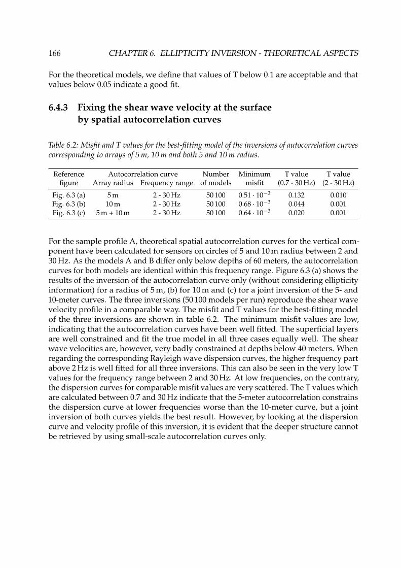
166 CHAPTER 6. ELLIPTICITY INVERSION - THEORETICAL ASPECTS

For the theoretical models, we define that values of T below 0.1 are acceptable and thatvalues below 0.05 indicate a good fit.

6.4.3 Fixing the shear wave velocity at the surfaceby spatial autocorrelation curves

Table 6.2: Misfit and T values for the best-fitting model of the inversions of autocorrelation curvescorresponding to arrays of 5 m, 10 m and both 5 and 10 m radius.

Reference Autocorrelation curve Number Minimum T value T valuefigure Array radius Frequency range of models misfit (0.7 - 30 Hz) (2 - 30 Hz)

Fig. 6.3 (a) 5 m 2 - 30 Hz 50 100 0.51 · 10−3 0.132 0.010Fig. 6.3 (b) 10 m 2 - 30 Hz 50 100 0.68 · 10−3 0.044 0.001Fig. 6.3 (c) 5 m + 10 m 2 - 30 Hz 50 100 0.64 · 10−3 0.020 0.001

For the sample profile A, theoretical spatial autocorrelation curves for the vertical com-ponent have been calculated for sensors on circles of 5 and 10 m radius between 2 and30 Hz. As the models A and B differ only below depths of 60 meters, the autocorrelationcurves for both models are identical within this frequency range. Figure 6.3 (a) shows theresults of the inversion of the autocorrelation curve only (without considering ellipticityinformation) for a radius of 5 m, (b) for 10 m and (c) for a joint inversion of the 5- and10-meter curves. The three inversions (50 100 models per run) reproduce the shear wavevelocity profile in a comparable way. The misfit and T values for the best-fitting modelof the three inversions are shown in table 6.2. The minimum misfit values are low,indicating that the autocorrelation curves have been well fitted. The superficial layersare well constrained and fit the true model in all three cases equally well. The shearwave velocities are, however, very badly constrained at depths below 40 meters. Whenregarding the corresponding Rayleigh wave dispersion curves, the higher frequency partabove 2 Hz is well fitted for all three inversions. This can also be seen in the very low Tvalues for the frequency range between 2 and 30 Hz. At low frequencies, on the contrary,the dispersion curves for comparable misfit values are very scattered. The T values whichare calculated between 0.7 and 30 Hz indicate that the 5-meter autocorrelation constrainsthe dispersion curve at lower frequencies worse than the 10-meter curve, but a jointinversion of both curves yields the best result. However, by looking at the dispersioncurve and velocity profile of this inversion, it is evident that the deeper structure cannotbe retrieved by using small-scale autocorrelation curves only.

6.4. TESTS ON THEORETICAL DATA 167

(a)

(b)

(c)

Figure 6.3: (a) Results for the inversion of the theoretical autocorrelation curve (left, with datapoints in black) for a ring with a 5 meter radius: Dispersion curves (center left), and shearwave (center right) velocity profiles. A zoom to the shallow structure of the shear wave velocityprofiles is displayed at right. All models generated during the inversion process with misfit valueslower than 1 are shown in the color of the respective misfit value. Darker curves are associatedwith higher misfit values, whereas lighter colors indicate the best-fitting models. The black linecorresponds to the actual soil model. (b) The same as (a), but for a ring with a radius of 10 meters.(c) The same for a joint inversion of the 5-meter-ring (autocorrelation curve top left) and the10-meter ring (autocorrelation curve bottom left).

168 CHAPTER 6. ELLIPTICITY INVERSION - THEORETICAL ASPECTS

6.4.4 Which parts of the ellipticity curve are necessaryfor the inversion process?

The deeper part of the structure can be fixed by using Rayleigh wave ellipticity measure-ments. In the following inversions, the theoretical autocorrelation curve for a radius of5 m (between 2 and 30 Hz) and the theoretical ellipticity curves of profiles A and B willbe inverted jointly. In order to determine which parts of the ellipticity curve carry theimportant information about the soil structure, different parts of the ellipticity curve willbe used for the inversion process and the results will be compared for both a model withand without singularities (peak and trough) in the ellipticity curve.

6.4.4.1 Model with a singularity in the ellipticity curve

Table 6.3: Parts of the autocorrelation and ellipticity curves used for the inversions and theassociated misfit and T values for the best-fitting models of joint inversions of autocorrelation andellipticity curves for model A.

Reference Autocorrelation curve Used frequency range Number Minimum T valuefigure Array radius Frequency range of the ellipticity curve of models misfit (0.7 - 30 Hz)

Fig. 6.4 (a) 5 m 2 - 30 Hz 0.2 - 0.65 Hz 100 100 8.5 · 10−3 0.241Fig. 6.4 (b) 5 m 2 - 30 Hz 0.7 - 2.0 Hz 100 100 15.4 · 10−3 0.043Fig. 6.4 (c) 5 m 2 - 30 Hz 0.2 - 2.0 Hz 150 200 30.2 · 10−3 0.140Fig. 6.4 (d) 5 m 2 - 30 Hz 0.7 - 4.0 Hz 150 200 21.2 · 10−3 0.087Fig. 6.4 (e) 5 m 2 - 30 Hz 0.7 - 1.7, 2.5 - 4.0 Hz 100 100 4.1 · 10−3 0.013Fig. 6.4 (f) 5 m 2 - 30 Hz 0.9 - 1.7, 2.5 - 4.0 Hz 100 100 3.9 · 10−3 0.016Fig. 6.4 (g) 5 m 2 - 30 Hz 0.9 - 1.7 Hz 100 100 7.0 · 10−3 0.154Fig. 6.4 (h) 10 m 2 - 30 Hz 0.9 - 1.7 Hz 100 100 1.1 · 10−3 0.030Fig. 6.4 (i) 5 m 2 - 30 Hz 0.7 - 4.0 Hz 150 200 35.7 · 10−3 0.093

Figure 6.4 (a) shows the results for an inversion of the left flank of the resonance peakonly, i.e. low-frequency ellipticity values between 0.2 and 0.65 Hz. The generated ellip-ticity curves are badly constrained above the peak frequency and the dispersion curvesexhibit a large variability over the whole frequency range. The true shear wave velocityprofile is not matched at all and the T value is large. However, the low minimum misfitvalue indicates that the used part of the ellipticity curve and the autocorrelation curveare well fitted.The inversion of the right flank of the ellipticity peak between 0.7 and 2 Hz (figure 6.4 (b))yields rather good results. Although only the right flank of the ellipticity peak is inverted,the left flank is well retrieved as well. Beyond the trough frequency, the ellipticity curve isnot well retrieved. The real dispersion curve is well retrieved and the shear wave velocityprofiles are well fitted as well. Unsurprisingly, the bedrock velocity is not retrieved.Combining both previous inversions by inverting the whole ellipticity peak (i.e. a fre-quency range from 0.2 to 2 Hz) gives an astonishing result (see figure 6.4 (c)). Althoughmore models have been generated in this case (150 200), the results are worse than for theinversion of the right flank only. The dispersion curves show a significant deviation from

6.4. TESTS ON THEORETICAL DATA 169

the true curve around 4.0 Hz. The shear wave velocity profile is not well constrained andthe bedrock depth underestimated. The comparatively large misfit value indicates thatthe inversion process is slowing down in the presence of very high ellipticity values andthe best model has not yet been found.An inversion of the part of the ellipticity curve from 0.7 to 4.0 Hz, including the right flankof the peak and the trough (figure 6.4 (d)), matches the ellipticity curve very well, also athigher frequencies. Here, 150 200 models have been generated as well, but the minimummisfit value is still relatively high, indicating that a prolongated search for better modelsmight have been successful. The T value of the best model proves the acceptable fit ofthe real dispersion curve, but the shear wave velocity profile’s discontinuity depths areunderestimated.In figure 6.4 (e), the same frequency range as in (d) was inverted, omitting ellipticitiesaround the trough frequency. The inverted frequency range lies between 0.7 and 1.7 andbetween 2.5 and 4.0 Hz. The minimum misfit and the associated T value are smaller thanin (d). The dispersion curve and the shear wave velocity profile are very well retrieved.The inversion is less time-consuming than in (d) and yields better results.In figure 6.4 (f), a smaller part of (e) was inverted, omitting ellipticity values exceeding 3.The frequency range of the inverted ellipticity data lies between 0.9 and 1.7 and between2.5 and 4.0 Hz. The inversion has misfit and T values comparable to (e).The same part of the right flank (0.9 - 1.7 Hz) without the data points at higher frequencieswas inverted in figure 6.4 (g). Despite the small misfit value, the T value is not acceptable.The ellipticity curve at frequencies above the trough is badly fitted. The dispersion curveand the velocity profile are badly retrieved as well. The deviation in the dispersion curvearound 4.0 Hz suggests that the overlap of the autocorrelation and ellipticity informationare not sufficient in this case.Therefore, in figure 6.4 (h), the autocorrelation for the 5-m ring has been replaced by the10-m ring autocorrelation curve, but the ellipticity data is the same as in (g). Here, themisfit and T values are very small, as the dispersion curve and the shear wave velocityprofile are very well retrieved.In real data measurements, the ellipticity trough is sometimes not retrieved due to contri-butions of Love waves or higher Rayleigh wave modes. Such effects are investigated infigure 6.4 (i), where an ellipticity curve with wrong data is inverted. The ellipticity partsused for inversion (e), i.e. the true ellipticity curve between 0.7 and 1.7 and between2.5 and 4.0 Hz, have been used. Instead of excluding the trough area, the data pointsbetween 1.7 and 2.5 Hz have been interpolated. The inversion succeeds in finding a soilmodel which exhibits a clear ellipticity peak, but no trough. The inversion result is stillacceptable and the T value comparable with the one of inversion (d), where the correctellipticity curve in the same frequency range was inverted. Nevertheless, inversion (e),where the data points between 2.5 and 4.0 Hz have been omitted, gives the best result.The theoretical ellipticity curve of model A exhibits a peak at 0.67 Hz and a trough at2.05 Hz. The parts of the ellipticity curve for the following inversions will be chosen inrelation with these two frequencies. Unless otherwise stated, the following results wereobtained after generating 100 100 soil models. The Rayleigh wave dispersion curve forfrequencies below the resonance frequency is dominated by the shear wave velocity inthe bedrock and the ellipticity curve is not sensitive to this velocity.

170 CHAPTER 6. ELLIPTICITY INVERSION - THEORETICAL ASPECTS

(a)

(b)

(c)

(d)

Figure 6.4: (a) Inversion results for joint inversions of the autocorrelation curve (left) and theellipticity curve (center left): dispersion curves (center right) and shear wave velocity profiles(right). For the inversion, the used data points are shown as black dots, the curves correspondingto the real model are shown as black lines: Inversion of the ellipticity curve (a) between 0.2 and0.65 Hz, (b) between 0.7 and 2 Hz, (c) between 0.2 and 2 Hz. (d) between 0.7 and 4 Hz.

6.4. TESTS ON THEORETICAL DATA 171

(e)

(f)

(g)

(h)

Figure 6.4: – continued. Inversion of the ellipticity curve (e) between 0.7 and 1.7 and 2.5 and4.0 Hz, (f) between 0.9 and 1.7 and 2.5 and 4.0 Hz, (g) between 0.9 and 1.7 Hz, (h) between 0.9and 1.7 Hz using the autocorrelation curve for the 10-m ring.

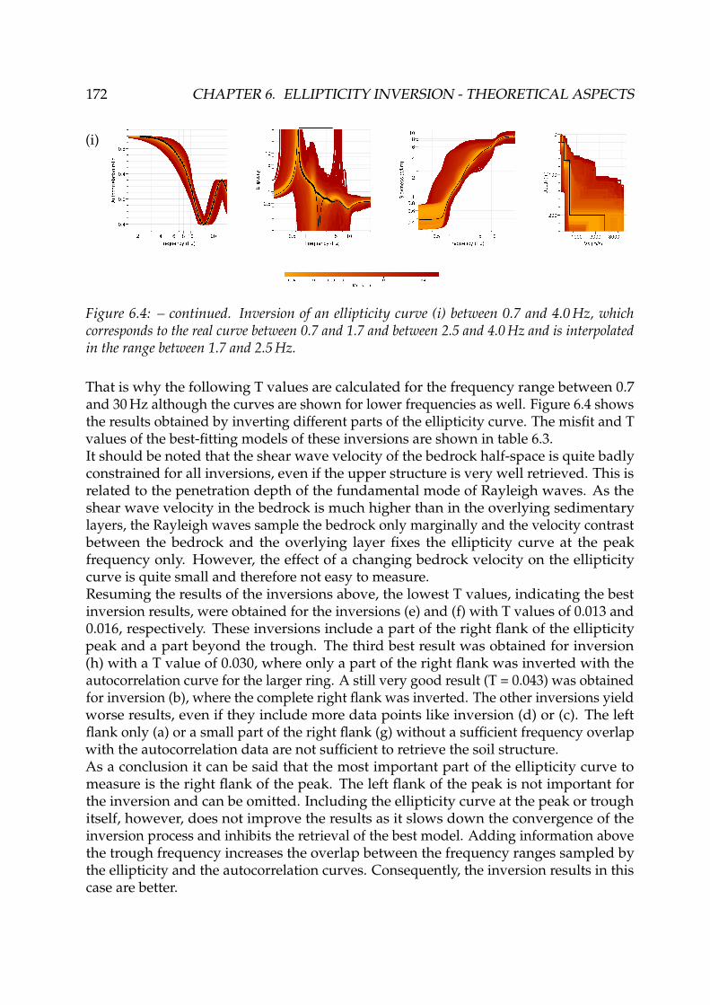
172 CHAPTER 6. ELLIPTICITY INVERSION - THEORETICAL ASPECTS

(i)

Figure 6.4: – continued. Inversion of an ellipticity curve (i) between 0.7 and 4.0 Hz, whichcorresponds to the real curve between 0.7 and 1.7 and between 2.5 and 4.0 Hz and is interpolatedin the range between 1.7 and 2.5 Hz.

That is why the following T values are calculated for the frequency range between 0.7and 30 Hz although the curves are shown for lower frequencies as well. Figure 6.4 showsthe results obtained by inverting different parts of the ellipticity curve. The misfit and Tvalues of the best-fitting models of these inversions are shown in table 6.3.It should be noted that the shear wave velocity of the bedrock half-space is quite badlyconstrained for all inversions, even if the upper structure is very well retrieved. This isrelated to the penetration depth of the fundamental mode of Rayleigh waves. As theshear wave velocity in the bedrock is much higher than in the overlying sedimentarylayers, the Rayleigh waves sample the bedrock only marginally and the velocity contrastbetween the bedrock and the overlying layer fixes the ellipticity curve at the peakfrequency only. However, the effect of a changing bedrock velocity on the ellipticitycurve is quite small and therefore not easy to measure.Resuming the results of the inversions above, the lowest T values, indicating the bestinversion results, were obtained for the inversions (e) and (f) with T values of 0.013 and0.016, respectively. These inversions include a part of the right flank of the ellipticitypeak and a part beyond the trough. The third best result was obtained for inversion(h) with a T value of 0.030, where only a part of the right flank was inverted with theautocorrelation curve for the larger ring. A still very good result (T = 0.043) was obtainedfor inversion (b), where the complete right flank was inverted. The other inversions yieldworse results, even if they include more data points like inversion (d) or (c). The leftflank only (a) or a small part of the right flank (g) without a sufficient frequency overlapwith the autocorrelation data are not sufficient to retrieve the soil structure.As a conclusion it can be said that the most important part of the ellipticity curve tomeasure is the right flank of the peak. The left flank of the peak is not important forthe inversion and can be omitted. Including the ellipticity curve at the peak or troughitself, however, does not improve the results as it slows down the convergence of theinversion process and inhibits the retrieval of the best model. Adding information abovethe trough frequency increases the overlap between the frequency ranges sampled bythe ellipticity and the autocorrelation curves. Consequently, the inversion results in thiscase are better.

6.4. TESTS ON THEORETICAL DATA 173

The best results for real data inversions can be expected if the whole right flank ismeasured accurately. If the complete flank cannot be measured, a part beyond the troughfrequency has to be included into the inversion process. However, if the trough frequencycannot be clearly measured, the ellipticity values in the questionable frequency range ofthe trough should be omitted.

6.4.4.2 Model without a singularity in the ellipticity curve

Table 6.4: Parts of the autocorrelation and ellipticity curves used for the inversions and theassociated misfit and T values for the best-fitting models of joint inversions of autocorrelation andellipticity curves for model B.

Figure Autocorrelation curve Ellipticity Number Minimum T valuereference Array radius Frequency range curve of models misfit (0.7 - 30 Hz)

Fig. 6.5 (a) 5 m 2 - 30 Hz 0.75 - 9.5 Hz 100 100 7.0 · 10−3 0.017Fig. 6.5 (b) 5 m 2 - 30 Hz 0.75 - 5.2 Hz 100 100 13.1 · 10−3 0.047Fig. 6.5 (c) 5 m 2 - 30 Hz 0.60 - 2.7 Hz 100 100 17.8 · 10−3 0.233

Model B does not exhibit an ellipticity singularity. The ellipticity curve shows a maximumof 1.71 at 0.73 Hz and a minimum of 0.36 at 9.44 Hz. Its ellipticity peak is broad andexhibits a sort of fine structure which is probably related to the different layer boundaries,but certainly not in a simple way. In order to determine which parts of the ellipticity curvehave to be included in the inversion process in this case, we performed joint inversionsof autocorrelation and ellipticity measurements. The theoretical autocorrelation curvefor a distance of 5 m was used jointly with different parts of the ellipticity curve of modelB. 100 100 models have been computed per inversion. The misfit and T values for thebest-fitting models are shown in table 6.4.Figure 6.5 (a) shows the results for an inversion of the right side of the broad ellipticitypeak between 0.75 and 9.5 Hz. The ellipticity curve is well fitted, the dispersion curveand the shear wave velocity profile are retrieved. This is also indicated by the low Tvalue.Inverting the right side of the ellipticity peak between 0.75 and 5.2 Hz yields good results(see figure 6.5 (b)). The dispersion curve is well retrieved, but slight uncertainties in theestimation of the shear wave velocity profile can be seen.Using the ellipticity values between 0.6 and 2.7 Hz only is not sufficient to find the correctsoil structure (figure 6.5 (c)). The ellipticity at higher frequencies is badly estimated andthe dispersion curve and velocity profile are badly fitted as well, although the minimummisfit value is in the same order as for the other inversions.These inversions prove that even in the case of an ellipticity which does not show a clearpeak or singularities, the ellipticity curve carries important information on the groundstructure and can be used to find the soil structure. The best results are obtained byinverting the complete right side of the ellipticity peak.

174 CHAPTER 6. ELLIPTICITY INVERSION - THEORETICAL ASPECTS

(a)

(b)

(c)

Figure 6.5: (a) Inversion results for joint inversions of the autocorrelation curve (left) and theellipticity curve (center left): dispersion curve (center right) and shear wave velocity profile(right). For the inversion used data points as black dots, the curves corresponding to the realmodel are shown as black lines: Inversion of the ellipticity curve (a) between 0.75 and 9.5 Hz, (b)between 0.75 and 5.2 Hz, (c) between 0.6 and 2.7 Hz.

6.4. TESTS ON THEORETICAL DATA 175

6.4.4.3 Joint inversion of dispersion and ellipticity curves

Table 6.5: Table of the misfit and T values for the best-fitting models of joint inversions of a part ofthe dispersion curve and a part of the ellipticity curve of model A.

Figure Dispersion Ellipticity Number Minimum T valuereference curve curve of models misfit (0.7 - 30 Hz)

Fig. 6.6 (a) 2 - 30 Hz 0.7 - 2.0 Hz 100 100 20.4 · 10−3 0.015Fig. 6.6 (b) 4 - 30 Hz 0.7 - 2.0 Hz 100 100 18.4 · 10−3 0.079Fig. 6.6 (c) 8 - 30 Hz 0.7 - 1.7, 2.5 - 4.0 Hz 100 100 4.1 · 10−3 0.019Fig. 6.6 (d) 10 - 30 Hz 0.7 - 1.7, 2.5 - 4.0 Hz 100 100 8.2 · 10−3 0.092

The previous subsections dealt with joint inversions of autocorrelation and ellipticitycurves. However, for an autocorrelation curve the frequency range where it really carriesinformation is connected to the descending flank of the plateau of the Bessel functionand therefore linked to its first root. Though, the exact frequency range where the auto-correlation curve carries information is not easy to determine. In the previous examples,the autocorrelation curve was used between 2 and 30 Hz. For a radius of 5 meters, thefirst zero-crossing of the autocorrelation occurs at 10 Hz, for the 10-meter ring it occursaround 7 Hz. As can be seen in figures 6.4 (g) and (h), it is evident that the 10-meterautocorrelation curve carries more information at low frequencies and constrains thevelocity profile to greater depths.SPAC is only one of the possible methods to measure Rayleigh wave dispersion curves.Another widespread method of measuring is MASW [Park et al., 1999, Socco and Strob-bia, 2004]. These active measurements yield high-frequency dispersion curves. Thecombination of existing MASW mesurements with ellipticity measurements obtainedusing a single station would be a simple way of extending the knowledge of the soilstructure to larger depths. It is clear that the joint inversion cannot succeed if the fre-quency ranges of the ellipticity and dispersion curves are too separated. Therefore, theobjective of this subsection is to determine how close they really have to be.In figure 6.6, the results of joint inversions of ellipticity and dispersion curves are shown.Each figure was obtained by generating 100 100 models. The minimum misfit and Tvalues of the inversions are shown in table 6.5. In figure 6.6 (a) and (b), the ellipticitydata correspond to those used in figure 6.4 (b), in 6.6 (c) and (d), the ellipticity data arethose of figure 6.4 (e). One could argue that the calculation of the T value for an inversionof dispersion curves is the same as the calculation of the misfit. If the ellipticity datawas not included in the inversion, this would be true. However, only a small part ofthe dispersion curve is used here and the remaining parts of the dispersion curve areconstrained by the ellipticity curve. Therefore, the T value is still appropriate to assessthe goodness of the inversion result.

176 CHAPTER 6. ELLIPTICITY INVERSION - THEORETICAL ASPECTS

(a)

(b)

(c)

(d)

Figure 6.6: (a) Inversion results for joint inversions of the ellipticity curve (left) and the dispersioncurve (center): resulting shear wave velocity profile (right). For the inversion used data pointsas black dots, the curves corresponding to the real model are shown as black lines: Inversion ofthe ellipticity curve between 0.7 and 2 Hz and the dispersion curve (a) between 2 and 30 Hz, (b)between 4 and 30 Hz, (c) between 6 and 30 Hz. Inversion of the ellipticity curve between 0.7 and1.7 Hz and between 2.5 and 4 Hz and the dispersion curve (d) between 8 and 30 Hz, (e) between10 and 30 Hz.

6.4. TESTS ON THEORETICAL DATA 177

The first two inversions (figures 6.6 (a) and (b)) show the results for inverting the elliptic-ity curve between 0.7 and 2 Hz with different parts of the dispersion curve. Combiningthe ellipticity information with the dispersion curve between 2 and 30 Hz yields thecorrect soil structure. The T value of this inversion is better than the one for the inversionof figure 6.4 (b), where the autocorrelation curve was inverted instead of the dispersioncurve. The correct dispersion curve is matched.By restricting the dispersion curve to the range between 6 and 30 Hz (figure 6.6 (b)) theresult degrades. The velocity profile is not well retrieved any more. The dispersioncurve is still acceptably fitted, but the T value is five times the value of (a), althoughthe minimum misfit is comparable. Omitting more dispersion curve data subsequentlyworsens the results.Using the same ellipticity data as in figure 6.4 (e), i.e. between 0.7 and 1.7 and between2.5 and 4 Hz, covers a wider frequency range. Consequently, the dispersion curve can belimited to higher frequencies. In this case, inverting the ellipticity curve jointly with thedispersion curve between 8 and 30 Hz is sufficient to retrieve the soil structure (figure 6.6(a)). The fit of the dispersion curve is very good with a low T value.However, using the dispersion curve between 10 and 30 Hz only (figure 6.6 (d)) gives aworse result. Although the inverted data are well fitted as well, the soil structure matchesbadly. The T value of the dispersion curve fit is still acceptable, but five times worse thanin the previous case.The examples above show that, in order to perform a successful joint inversion, thedistinct datasets do not necessarily need to have an overlap in the frequency domain.Combining ellipticity data below 4 Hz with a dispersion curve above 8 Hz retrieves thecorrect soil structure. However, a further increase of this gap deteriorates the resultsuntil the two distinctive data sets are not linked any more. Beyond that point, a suc-cessful inversion becomes impossible. Furthermore, this result shows that the ellipticityand dispersion curve carry information about the same superficial layers at differentfrequencies. Otherwise, it would be impossible to invert a high-frequency dispersioncurve measurement and a low-frequency ellipticity curve jointly, with both curves beingdefined in distinct, non-overlapping frequency ranges.

6.4.5 Inversion of erroneous ellipticity curves

The measurement of ellipticity curves can always be biased by systematic errors, intro-duced for example by a wrong estimation of the amount of Love waves or incompleteelimination of waves other than Rayleigh waves. In this subsection, the same autocor-relation curve as in the previous subsections will be inverted jointly with a wronglyestimated ellipticity curve of model A. As in subsection 6.4.4.1 the inversion of theellipticity curve parts between 0.7 and 1.7 and 2.5 and 4 Hz gave the best results, onlythese parts will be used for the inversion here. The inversion shown in figure 6.4 (e) willtherefore be taken as reference inversion.

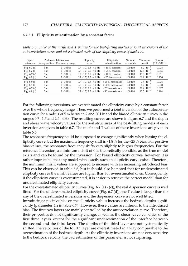
178 CHAPTER 6. ELLIPTICITY INVERSION - THEORETICAL ASPECTS

6.4.5.1 Ellipticity misestimation by a constant factor

Table 6.6: Table of the misfit and T values for the best-fitting models of joint inversions of theautocorrelation curve and misestimated parts of the ellipticity curve of model A.

Figure Autocorrelation curve Ellipticity Ellipticity Number Minimum T valuereference Array radius Frequency range curve misestimation of models misfit (0.7 - 30 Hz)

Fig. 6.7 (a) 5 m 2 - 30 Hz 0.7 - 1.7, 2.5 - 4.0 Hz + 10 % constant 100 100 6.2 · 10−3 0.028Fig. 6.7 (b) 5 m 2 - 30 Hz 0.7 - 1.7, 2.5 - 4.0 Hz + 25 % constant 100 100 12.5 · 10−3 0.055Fig. 6.7 (c) 5 m 2 - 30 Hz 0.7 - 1.7, 2.5 - 4.0 Hz + 40 % constant 100 100 15.9 · 10−3 0.051Fig. 6.7 (d) 5 m 2 - 30 Hz 0.7 - 1.7, 2.5 - 4.0 Hz - 25 % constant 100 100 60.9 · 10−3 0.150

Fig. 6.9 (a) 5 m 2 - 30 Hz 0.7 - 1.7, 2.5 - 4.0 Hz + 25 % maximum 100 100 7.4 · 10−3 0.026Fig. 6.9 (b) 5 m 2 - 30 Hz 0.7 - 1.7, 2.5 - 4.0 Hz + 50 % maximum 100 100 8.0 · 10−3 0.038Fig. 6.9 (c) 5 m 2 - 30 Hz 0.7 - 1.7, 2.5 - 4.0 Hz - 25 % maximum 100 100 26.4 · 10−3 0.097Fig. 6.9 (d) 5 m 2 - 30 Hz 0.7 - 1.7, 2.5 - 4.0 Hz - 50 % maximum 100 100 85.5 · 10−3 0.194

For the following inversions, we overestimated the ellipticity curve by a constant factorover the whole frequency range. Then, we performed a joint inversion of the autocorrela-tion curve for a radius of 5 m between 2 and 30 Hz and the biased ellipticity curves in theranges 0.7 - 1.7 and 2.5 - 4 Hz. The resulting curves are shown in figure 6.7 and the depthand shear wave velocity values for the soil structures of the best-fitting models of eachinversion are given in table 6.7. The misfit and T values of these inversions are given intable 6.6.The resonance frequency could be supposed to change significantly when biasing the el-lipticity curve, but the maximum frequency shift is - 1.8 % for the - 25 % bias. For positivebias values, the resonance frequency shifts very slightly to higher frequencies. For thereference inversion, a minimum misfit of 0 is theoretically possible, as the true modelexists and can be found by the inversion. For biased ellipticity curves, however, it israther improbable that any model with exactly such an ellipticity curve exists. Therefore,the minimum misfit values are supposed to increase with an increasing introduced bias.This can be observed in table 6.6, but it should also be noted that for underestimatedellipticity curves the misfit values are higher than for overestimated ones. Consequently,if the ellipticity curve is overestimated, it is easier to retrieve the correct model than forunderestimated ellipticity curves.For the overestimated ellipticity curves (Fig. 6.7 (a) - (c)), the real dispersion curve is wellfitted. For the underestimated ellipticity curve (Fig. 6.7 (d)), the T value is larger than forany of the overestimated inversions and the dispersion curve is not well fitted.Introducing a positive bias on the ellipticity values increases the bedrock depths signifi-cantly (parameter D4 in table 6.7). However, these values are inferior to the introducedbias. The first two layers are mainly controlled by the autocorrelation curve. Therefore,their properties do not significantly change, as well as the shear wave velocities of thefirst three layers, except for the significant underestimation of the interface betweenthe second and the third layer. The depths of the third layer are not systematicallyshifted, the velocities of the fourth layer are overestimated in a way comparable to theoverestimation of the bedrock depth. As the ellipticity inversions are not very sensitiveto the bedrock velocity, the bad estimation of this parameter is not surprising.

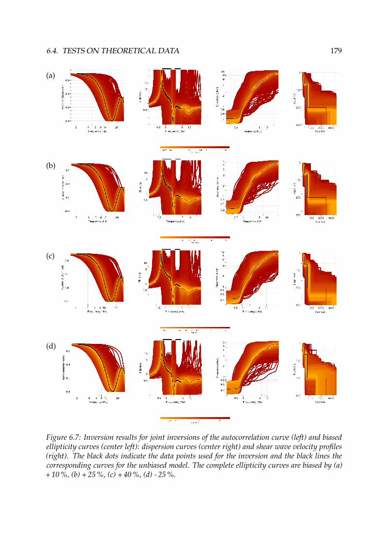
6.4. TESTS ON THEORETICAL DATA 179

(a)

(b)

(c)

(d)

Figure 6.7: Inversion results for joint inversions of the autocorrelation curve (left) and biasedellipticity curves (center left): dispersion curves (center right) and shear wave velocity profiles(right). The black dots indicate the data points used for the inversion and the black lines thecorresponding curves for the unbiased model. The complete ellipticity curves are biased by (a)+ 10 %, (b) + 25 %, (c) + 40 %, (d) - 25 %.

180 CHAPTER 6. ELLIPTICITY INVERSION - THEORETICAL ASPECTS

Overall, it can be stated that the superficial structure, mainly controlled by the autocorre-lation curve, is quite robust against overestimation of the ellipticity. The overestimation ofthe deeper structure, particularly the parameters of the layer directly above the bedrock,is still smaller than the bias on the real ellipticity curve.Introducing a negative bias of - 25 % on the ellipticity values, however, gives a differentresult. The velocity of the superficial layer stays constant, but every parameter from thefirst layer’s depth to the shear wave velocity of the fourth layer is shifted by approxi-mately - 10 % (ranging from - 7.0 to - 12.0 %). The bedrock depth is underestimated byonly - 3.9 %. The ellipticity underestimation also influences the superficial structure, butthe bias induced in the whole structure is far below the introduced ellipticity bias.The percental deviation of the bedrock depth D4, the mean velocity vSB and the shearwave travel time τSB between the surface and the bedrock depth are plotted as a functionof the percental ellipticity misestimation in figure 6.8. The travel time calculation is basedon the shear wave velocities and layer depths. The mean velocity is calculated as theratio between the bedrock depth and the travel time. The travel time values vary onlyslightly with varying ellipticity bias. The increasing travel-time for the underestimatedellipticity curve is against the trend of the overestimated ellipticity values. In any case,the variations of the travel time (maximum 5.7 %) are much lower than the introducedellipticity bias. The bedrock depth and mean velocity are more sensitive to the ellipticitymisestimation. The scaling of soil profiles itself does not change travel times, but velocityand depth parameters of the single layers, and do provide very close site reponses.

−60 −40 −20 0 20 40 60−30

−20

−10

0

10

20

30

Ellipticity bias [%]

Fin

al e

stim

atio

n bi

as [%

]

D4 for constant bias

vSB

for constant bias

τSB

for constant bias

D4 for variable bias

vSB

for variable bias

τSB

for variable bias

Figure 6.8: Percental deviation of bedrock depth D4, mean velocity vSB and shear wave traveltime τSB from the surface to the bedrock in function of the introduced bias on the ellipticitycurve. The results for a constant ellipticity misestimation are shown in dark color, for a variablemisestimation in light color. For the variable misestimation, the x-axis indicates the maximumellipticity deviation.

6.4. TESTS ON THEORETICAL DATA 181

6.4.5.2 Frequency-dependent ellipticity misestimation

For the following inversions, the autocorrelation and ellipticity curves are inverted overthe same frequency ranges as in the previous case, but the systematic error imposedon the ellipticity curve is frequency-dependent in the following way: At 0.7 Hz, theellipticity value is not biased. At 1.7 Hz and between 2.5 and 4 Hz, the bias equals + 25 %,+ 50 %, - 25 % and - 50 %. Between 0.7 and 1.7 Hz, the bias changes continuously. Theoverestimated cases are more representative for real ellipticity measurements than inthe previous inversions as low ellipticities are more susceptible to overestimations thanhigher ellipticity values because an overestimation of the horizontal displacement dueto Love waves has less impact if the horizontal Rayleigh wave displacement, and thusthe ellipticity, is high. The results are shown in figure 6.9 and the depth and shear wavevelocity values for the soil structures of the best-fitting models of each inversion aregiven in table 6.7. The minimum misfit and T values are given in table 6.6.Ellipticity over- and underestimations both yield positive resonance frequency shifts,although the relative error is very small for overestimated ellipticities and acceptable forunderestimated ellipticities.Adding a positive bias of maximum + 25 % leads to misestimations of single propertieslower than 10 %. In the case where the ellipticity curve is biased by at most + 50 %, themisestimation of the layer properties is lower than 17 %. In both cases, the dispersioncurve is still well fitted.Underestimating the ellipticity curves reveals a different picture. In both cases, thedispersion curve is not well retrieved. Except for the surface velocity, even the propertiesof the shallow layers are misestimated by over 10 %. The deeper layers are misestimatedby up to 17.5 % (-25 % bias) and 30.0 % (-50 % bias). In these two cases, yet the autocorre-lation curves do not seem perfectly fitted.The percental deviations of the bedrock depth, the mean velocity and the shear wavetravel time for frequency-dependent ellipticity misestimations are plotted in figure 6.8.Here, the travel times are even less biased than in the case of a constant ellipticity bias.The bedrock depths and mean velocities vary in a systematic way, but the slope of thecorresponding curves is larger for negative ellipticity misestimations. This is furtherevidence indicating that the ellipticity inversion is more robust against overestimatedellipticity values than against underestimated ones.

182 CHAPTER 6. ELLIPTICITY INVERSION - THEORETICAL ASPECTS

(a)

(b)

(c)

(d)

Figure 6.9: Inversion results for joint inversions of the autocorrelation curve (left) and biasedellipticity curves (center left): dispersion curves (center right) and shear wave velocity profiles(right). The black dots indicate the data points used for the inversion and the black lines thecorresponding curves for the unbiased model. The ellipticity curves are biased by maximum (a)+ 25 %, (b) + 50 %, (c) - 25 %, (d) - 50 %.

6.4. TESTS ON THEORETICAL DATA 183

Tabl

e6.

7:Ta

ble

ofth

ela

yers

’dep

ths

and

shea

rw

ave

velo

citie

sfo

rth

em

odel

sw

ithlo

wes

tmis

fitva

lues

resu

lting

from

bias

edin

vers

ions

.A

lso

show

nar

eth

etr

avel

-tim

efr

omth

esu

rfac

eto

the

bedr

ock

τ SB

and

the

aver

age

velo

city

v SB

=D

4/τ S

Bof

the

sedi

men

tary

laye

rs.T

here

fere

nce

mod

elis

the

inve

rsio

nsh

own

infig

ure

6.4

(e).

The

bias

edm

odel

sfo

rth

eco

nsta

ntbi

ases

of+

10%

,+25

%,+

40%

and

-25

%ar

esh

own

infig

ures

6.7

(a),

(b),

(c)a

nd(d

),re

spec

tive

ly.T

hebi

ased

mod

els

for

the

freq

uenc

y-de

pend

entb

iase

sof

+25

%,+

50%

,-25

%an

d-5

0%

max

imum

are

show

nin

figur

es6.

9(a

),(b

),(c

)and

(d),

resp

ectiv

ely.

The

give

npe

rcen

tage

valu

esin

dica

teth

ede

viat

ion

ofth

ebe

st-fi

ttin

gm

odel

s’va

lues

from

the

real

mod

elva

lues

.

Figu

reV

S1D

1V

S2D

2V

S3D

3V

S4D

4V

S5f 0

τ SB

v SB

refe

renc

e[m

/s]

[m]

[m/

s][m

][m

/s]

[m]

[m/

s][m

][m

/s]

[Hz]

[s]

[m/

s]

mod

el12

0.0

5.0

200.

020

.032

0.0

65.0

625.

020

0.0

2500

.00.

668

0.47

342

2.6

refe

renc

eFi

g.6.

4(e

)11

9.6

4.96

198.

719

.631

3.0

64.7

625.

919

7.3

2442

.50.

671

0.47

141

8.8

mod

el-0

.3%

-0.8

%-0

.7%

-2.0

%-2

.2%

-0.5

%+

0.1

%-1

.4%

-2.3

%+

0.4

%-0

.4%

-0.9

%

+10

%Fi

g.6.

7(a

)12

0.8

4.91

200.

719

.431

9.3

68.3

698.

321

4.7

3040

.20.

667

0.47

645

1.4

cons

tant

+0.

7%

-1.8

%+

0.4

%-3

.0%

-0.2

%+

5.1

%+

11.7

%+

7.4

%+

21.6

%-0

.1%

+0.

6%

+6.

8%

+25

%Fi

g.6.

7(b

)11

9.6

4.87

194.

817

.129

4.8

64.5

726.

722

3.1

3494

.70.

672

0.48

346

2.4

cons

tant

-0.3

%-2

.6%

-2.6

%-1

4.5

%-7

.9%

-0.8

%+

16.3

%+

11.6

%+

39.8

%+

0.6

%+

2.1

%+

9.4

%+

40%

Fig.

6.7

(c)

120.

84.

8720

0.7

18.3

319.

369

.680

2.7

250.

133

91.9

0.67

50.

493

507.

5co

nsta

nt+

0.7

%-2

.6%

+0.

4%

-8.5

%-0

.2%

+7.

1%

+28

.4%

+25

.1%

+35

.7%

+1.

0%

+4.

2%

+20

.1%

-25

%Fi

g.6.

7(d

)11

9.6

4.54

179.

918

.628

3.3

58.2

550.

019

2.2

1515

.00.

656

0.50

038

4.8

cons

tant

-0.3

%-9

.2%

-10.

1%

-7.0

%-1

1.5

%-1

0.5

%-1

2.0

%-3

.9%

-39.

4%

-1.8

%+

5.7

%-8

.9%

+25

%Fi

g.6.

9(a

)11

9.6

4.82

194.

818

.130

6.8

64.6

671.

121

2.5

2567

.10.

670

0.48

044

2.3

max

imum

-0.3

%-3

.6%

-2.6

%-9

.5%

-4.1

%-0

.6%

+7.

4%

+6.

3%

+2.

7%

+0.

3%

+1.

5%

+4.

7%

+50

%Fi

g.6.

9(b

)12

0.8

4.96

204.

718

.532

2.4

68.3

726.

723

3.3

2618

.70.

669

0.48

947

7.4

max

imum

+0.

7%

-0.8

%+

2.4

%-7

.5%

+0.

8%

-5.1

%+

16.3

%+

16.7

%+

4.7

%+

0.1

%+

3.4

%+

13.0

%-2

5%

Fig.

6.9

(c)

118.

44.

1917

4.6

17.6

283.

356

.452

3.3

165.

130

10.1

0.67

00.

457

361.

3m

axim

um-1

.3%

-16.

2%

-12.

7%

-12.

0%

-11.

5%

-13.

2%

-16.

3%

-17.

5%

+20

.4%

+0.

3%

-3.4

%-1

4.5

%-5

0%

Fig.

6.9

(d)

124.

54.

4515

3.4

16.0

261.

648

.143

7.5

140.

828

92.7

0.67

40.

446

315.

9m

axim

um+

3.8

%-1

1.0

%-2

3.3

%-2

0.0

%-1

8.3

%-2

6.0

%-3

0.0

%-2

9.6

%+

15.7

%+

0.9

%-5

.7%

-25.

2%

184 CHAPTER 6. ELLIPTICITY INVERSION - THEORETICAL ASPECTS

6.5 Conclusion

This paper showed the theoretical possibilities, constraints and limits of inversions in-cluding the Rayleigh wave ellipticity in order to retrieve the local soil structure. First ofall, it was shown that an inversion of an ellipticity curve must be performed jointly, e.g.with an autocorrelation or dispersion curve. The frequency ranges of both measurementsdo not necessarily have to overlap, but should be as close as possible. In the case ofan ellipticity curve with singularities, the ellipticity curve should be truncated in orderto exclude too high or too low values, which might strongly reduce the exploration ofthe complete parameter space. As the left flank of the ellipticity peak does not carryimportant information, the inversion should comprise only the frequency range abovethe peak frequency. If the ellipticity curve does not exhibit singularities, the completeright side of the peak which is, in general, broader than in the previous case has to beincluded in the inversion. For misestimated ellipticity curves, the induced errors in thesoil structure are, in general, smaller than the introduced bias (about half the originalbias).In the present paper, all ellipticity and autocorrelation curves were calculated theoreti-cally. For ellipticity curves obtained from real data measurements, a perfect measurementof the real ellipticity curve cannot be expected. Even if all contributions of other wavetypes are perfectly excluded, higher modes of Rayleigh waves can still bias the ellipticityestimation, especially at high frequencies. In the present study, these effects were disre-garded. The identification of such effects in the ellipticity curve, however, is impossiblein most cases. Therefore, it is advisable to limit the use of the ellipticity curve to the rightflank of the peak. Consequently, the station distance used for the autocorrelation mea-surements should be chosen as small as possible for a good resolution of the superficiallayers and in the same time as large as necessary for a good link between the frequencyranges of the ellipticity and autocorrelation curves. To estimate the correct array sizefor the autocorrelation measurements, preliminary information on the undergroundstructure have to be known or assumed (e.g. H/V resonance frequency, geology).Another problem with real data ellipticity curves is that the estimation of the propertiesof Rayleigh waves usually exploits the correlation between the vertical and the horizon-tal movement. Yet, at the singularities of the ellipticity curve, one of both componentsvanishes. Therefore, at those points, both components are not correlated any more. Con-sequently, at the trough frequency, the movement of Rayleigh and Love waves cannotbe distinguished any more (at least when using a single sensor) and the ellipticity willbe overestimated here. At the peak frequency, the vertical signal will be overestimatedin an analog way. Therefore, the ellipticity value will be underestimated here. Thus, itis advisable to exclude the ellipticity estimation around the singular values from theellipticity inversion.In the companion paper, the lessons learned in the present paper for the inversion ofellipticity curves will be used to invert real data measurements.

Chapter 7

Inversion of ellipticity curves -Application to real data measurements

In chapter 6, the theoretical aspects of the inversion of ellipticity curves have been pre-sented. It has been investigated which parts of the ellipticity curve are actually carryingthe information on the soil structure and which additional measurements are necessaryto make the inversion unambiguous. Furthermore, how misestimated ellipticity datainfluence the inversion result was shown. In this chapter, the lessons learned in chapter 6will be applied to real data measurements which have been performed during the Euro-pean NERIES project (2006-2010). The following text represents the article "Inversion ofRayleigh wave ellipticity measurements, Part II: Application to real data measurements"by Hobiger, Cornou, Di Giulio, Endrun, Renalier, Savvaidis, Bard, Hailemikael, Le Bihan,Ohrnberger, Theodulidis, and Wathelet, 2010b, which was submitted to Geophysical Jour-nal International.

Le chapitre 6 a présenté les aspects théoriques de l’inversion de courbes d’ellipticité. Il a étédéterminé quelles parts de la courbe d’ellipticité comportent les informations sur la structure dusol et quelles mesures additionnelles sont nécessaires afin de rendre l’inversion unique. En outre,l’influence de misestimations d’ellipticité sur le résultat d’inversion a été démontré. Dans lechapitre suivant, les leçons du chapitre 6 seront appliquées à des données réelles mesurées dansle cadre du projet européen NERIES (2006-2010). Le texte suivant représente l’article "Inversionof Rayleigh wave ellipticity measurements, Part II: Application to real data measurements" parHobiger, Cornou, Di Giulio, Endrun, Renalier, Savvaidis, Bard, Hailemikael, Le Bihan, Ohrnberger,Theodulidis, and Wathelet, 2010b, qui a été soumis à Geophysical Journal International.

185

186 CHAPTER 7. ELLIPTICITY INVERSION - REAL DATA

7.1 Abstract

Site effects can have a large impact on the damages occurring during earthquakes. There-fore, it is important to know the local soil structure in order to assess the seismic hazard.Established methods include borehole drilling and active reflection or refraction measure-ments. These measurements are, however, either expensive or not very appropriate forthe use in urban areas. Another way is to obtain the dispersion curves of surface wavesby measuring ambient seismic vibrations using arrays of seismic sensors. However, toensure a good depth coverage, the measurements have to be performed at several arraysizes or using a single array composed of a large number of stations. Therefore, suchmeasurements are time-consuming. A simple alternative is the use of Rayleigh waveellipticity, which can be measured by a single seismic sensor. Ellipticity as a functionof frequency is closely linked to the shear wave velocity profile. Though, the ellipticitycannot be inverted unambiguously because a scaling of the velocity profile does notchange the ellipticity curve. Therefore, additional measurements fixing the absolutevalues of the velocities at certain depths are necessary. Small scale SPAC or MASWmeasurements can provide this data. In a companion article, the theoretical aspects ofjoint inversions of ellipticity and SPAC or MASW measurements have been shown. Thisarticle applies the method to real data measurements collected at 14 different sites duringthe European NERIES project. It is found that the ellipticity inversion results are in goodagreement with dispersion curve measurements and that the determined Vs30 valuesagree with borehole measurements for most sites. Furthermore, the method can help inidentifying the mode of Rayleigh waves in dispersion curve measurements.

7.2 Introduction

The knowledge of the local soil structure is an important component of seismic hazardassessment as site effects can amplify ground motion and increase damages. Differentmethods permit the retrieval of the local soil properties, among them the drilling ofboreholes and seismic refraction or reflection measurements. These methods are quiteexpensive or hardly suitable for urban areas. Alternatively, the soil can be investigated bymeasurements which generate surface waves actively, e.g. by sledgehammering. As thehammering generates waves at high frequencies only, this method investigates the verysuperficial layers only [Socco and Strobbia, 2004]. Another way of measuring in urbanareas is to use ambient seismic vibrations which are generated by natural sources like theocean waves or by human activities like traffic or industry, depending on the frequencyrange. By deploying arrays of seismic sensors, the dispersion curves of Rayleigh andLove surface waves can be measured. In order to cover a large frequency band, how-ever, arrays of different sizes or a single array including many sensors have to be used[Wathelet, 2008]. Consequently, such measurements are time-consuming. By exploitingthe ellipticity of Rayleigh waves, the number of sensors needed for the measurementscan be reduced. The ellipticity indicates the ratio between the horizontal and the ver-tical movement of a Rayleigh wave and is a function of frequency. The possibility toconstrain the soil structure by ellipticity data was first shown by Boore and Toksöz [1969].

7.2. INTRODUCTION 187

A widespread technique used to characterize site effects is the H/V method which wasproposed by Nogoshi and Igarashi [1971] and promoted by Nakamura [1989]. Thismethod indicates the spectral ratio between the horizontal and the vertical components.If other wave types than Rayleigh waves did not contribute to the ambient noise spectra,the H/V curve would match the ellipticity curve. The exact composition of the noisewave field depends on the source characteristics of seismic noise and on the site structure[Bonnefoy-Claudet et al., 2008]. The main wave types are Rayleigh and Love waves, buttheir ratio is frequency-dependent or even time-dependent [Köhler et al., 2006, Endrun,2010]. As Love waves are only present on the horizontal components, the H/V ratio will,in general, misestimate ellipticity. Assuming an a priori proportion between Rayleighand Love waves, one can remove the Love wave contributions on the H/V ratio and useit as an ellipticity curve [Fäh et al., 2001, 2003]. Although the interpretation of H/V is stillcontroversial, previous studies have already shown the benefits of including H/V datato inversions of Rayleigh wave dispersion curves [for instance Scherbaum et al., 2003,Parolai et al., 2005, Picozzi et al., 2005, Arai and Tokimatsu, 2005]. Arai and Tokimatsu[2004] used H/V data to fix the exact depths of shallow layers where the shear wavevelocities were known by borehole measurements.Either the use of H/V curves is limited to the use of the resonance frequency only oradditional assumptions have to be made to correct other wave types’ contributionsif the whole curve is to be used. Newly developed methods exist which allow thedirect measurement of ellipticity curves. The RayDec method [Hobiger et al., 2009a]discriminates other waves than Rayleigh waves by statistical means for single seismicsensors. Poggi and Fäh [2010] propose a method using f-k analysis which can evenidentify higher modes using arrays of several seismic sensors.As scaling the depth and velocity properties of the soil structure by the same factor doesnot change the ellipticity curve [Scherbaum et al., 2003, companion paper], an inversionof ellipticity data alone will never yield the correct velocity profile. In order to fix theabsolute shear wave velocity values of the profile, additional measurements are needed.For this purpose, small scale spatial autocorrelation measurements using few seismicsensors [Aki, 1957] or MASW measurements [Park et al., 1999, Socco and Strobbia, 2004]can be used.A companion paper investigated the theoretical aspects of joint inversions of ellipticityand autocorrelation or dispersion curves in detail. It shows that the part of the ellipticitycurve which carries the important information is the right flank of the peak whetherthe ellipticity curve does exhibit a singularity or not. The exact ellipticity values at thepeak and trough frequencies of the curve are difficult to measure, but too high or too lowellipticity values can be omitted for the inversion without corrupting the results. Thefrequency ranges of the inverted ellipticity and autocorrelation curves do not necessarilyhave to overlap as long as the gap between them is not too large (see companion paper).If the ellipticity measurement is biased, the resulting errors on the final soil structureinversion results are, in general, smaller than the introduced bias.This article will focus on the application of the theory developed in the previous article.We invert the ellipticity curves for 14 sites investigated during the European NERIESproject.

188 CHAPTER 7. ELLIPTICITY INVERSION - REAL DATA

For a representative selection of five of them, the inversions will be shown in detail.SPAC measurements using all stations of the array and for a subset of stations only willbe jointly inverted with ellipticity curves for these sites. For the remaining sites, only themain results will be shown.

7.3 Measurement methodology

7.3.1 Ellipticity measurementsThe ellipticity measurements have been performed using the RayDec method [Hobigeret al., 2009a]. This method uses the data of a single 3-component seismic sensor to retrievethe ellipticity of Rayleigh waves. The algorithm is based on the random decrementtechnique which is commonly used to characterize the dynamic parameters of buildingsor other oscillatory systems. The 3-component signal is cut in small time windowsstarting at the positive zero-crossings of the vertical component. For each time window,the signal of the horizontal components is projected into the direction which maximizesthe correlation to the vertical component with a 90◦ phase shift which is typical ofRayleigh waves. Subsequently, the signals obtained in this way are stacked together andthe ratio between the horizontal and vertical movements is estimated by analyzing theenergy content of the vertical and horizontal stack. We will not describe the methodin more detail here, but refer the interested reader to the publication of Hobiger et al.[2009a].

7.3.2 Spatial autocorrelation measurements

As the ellipticity inversion cannot be successful without additional information, weneed to include further data in the inversion process. Aki [1957] introduced the spatialautocorrelation (SPAC) technique.

(a)

−10 −5 0 5 10

−5

0

5

Distance [m]

Dis

tanc

e [m

]

(b)

5 10 20

−0.5

0

0.5

1

Frequency [Hz]

Aut

ocor

rela

tion

ratio

8s−SPAC4s−SPAC

Figure 7.1: (a) Layout of the smallest seismic array deployed in Nestos. SPAC measurementswere performed using the correlations between the central and: all ring stations (8s-SPAC), thethree marked ring stations (4s-SPAC). (b) Results for 8s-SPAC and 4s-SPAC.

7.3. MEASUREMENT METHODOLOGY 189

This technique uses the correlation between different seismic sensors to retrieve thedispersion curve. However, the original layout imposed that the distances between eachstation pair are equal. Therefore, the seismic stations were to be deployed on a ringaround a central station. In addition, the number of seismic stations should be large toensure a wide coverage of azimuths for incoming waves. As such a layout is, due tospatial limitations, hardly feasible in urban areas, Bettig et al. [2001] further developpedthe spatial autocorrelation method by suppressing the need of equal distances. Themeasurement is now possible for rings with a certain thickness. In this way, SPACmeasurements are possible even for unsymmetric array layouts. The SPAC measurementspresented in this paper are obtained using this method. For the measurements performedduring the NERIES project, a total of 8 seismological stations [Earthdata acquisitionsystems equipped with 5s-Lennartz 3-component sensors, Endrun, 2010] were usedfor each array of sensors. One station served as central station whereas the other 7stations were deployed on a ring around it, more or less symmetric depending on localconstraints.Okada [2006] showed that an array layout with three ring stations surrounding a centralstation is sufficient for good results, independent of the azimuth distribution of theseismic noise field. This is illustrated in figure 7.1. An example array layout is shownin figure 7.1 (a), corresponding to one of the investigated sites (Nestos). The 7 ringstations have distances to the central station between 6.59 and 7.24 m. We used onehour of measurements recorded on all 8 stations simultaneously. A 7-station pair SPACmeasurement has been performed using only pairs consisting of the central and anyring station. The three marked stations on the ring build a good triangle around thecentral station and are between 7.09 and 7.24 m distant from it. The SPAC measurementsresulting of the correlation of these three stations with the central station are comparedto the 7-station SPAC in figure 7.1 (b). Both measurements yield qualitatively identicalresults, but the error bars are smaller when using more stations.Morikawa et al. [2004] suggested 2s-SPAC, a method using only two seismic stationsto perform SPAC measurements. In this way, the reference station is fixed whereas thesecond station changes its position during the measurement. This method presumes thatthe seismic noise wave field is stationary in time. Nevertheless, the focus of this paperis not to investigate the temporal stationarity of the wave field or the applicability ofthe 2s-SPAC method. However, the use of 2s-SPAC could further decrease the costs ofseismic surveys. In the following, we will show inversions of ellipticity curves measuredat the central station combined with SPAC measurements using all available stations aswell as for three station pairs only (i.e. the extreme cases).

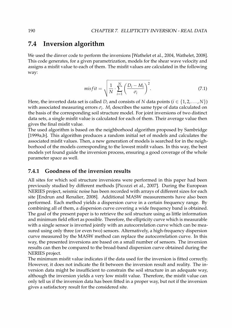
190 CHAPTER 7. ELLIPTICITY INVERSION - REAL DATA

7.4 Inversion algorithm

We used the dinver code to perform the inversions [Wathelet et al., 2004, Wathelet, 2008].This code generates, for a given parametrization, models for the shear wave velocity andassigns a misfit value to each of them. The misfit values are calculated in the followingway:

mis f it =

√√√√ 1N·

N

∑i=1

(Di −Mi

σi

)2

. (7.1)

Here, the inverted data set is called Di and consists of N data points (i ∈ {1, 2, . . . , N})with associated measuring errors σi. Mi describes the same type of data calculated onthe basis of the corresponding soil structure model. For joint inversions of two distinctdata sets, a single misfit value is calculated for each of them. Their average value thengives the final misfit value.The used algorithm is based on the neighborhood algorithm proposed by Sambridge[1999a,b]. This algorithm produces a random initial set of models and calculates theassociated misfit values. Then, a new generation of models is searched for in the neigh-borhood of the models corresponding to the lowest misfit values. In this way, the bestmodels yet found guide the inversion process, ensuring a good coverage of the wholeparameter space as well.

7.4.1 Goodness of the inversion results

All sites for which soil structure inversions were performed in this paper had beenpreviously studied by different methods [Picozzi et al., 2007]. During the EuropeanNERIES project, seismic noise has been recorded with arrays of different sizes for eachsite [Endrun and Renalier, 2008]. Additional MASW measurements have also beenperformed. Each method yields a dispersion curve in a certain frequency range. Bycombining all of them, a dispersion curve covering a wide frequency band is obtained.The goal of the present paper is to retrieve the soil structure using as little informationand minimum field effort as possible. Therefore, the ellipticity curve which is measurablewith a single sensor is inverted jointly with an autocorrelation curve which can be mea-sured using only three (or even two) sensors. Alternatively, a high-frequency dispersioncurve measured by the MASW method can replace the autocorrelation curve. In thisway, the presented inversions are based on a small number of sensors. The inversionresults can then be compared to the broad-band dispersion curve obtained during theNERIES project.The minimum misfit value indicates if the data used for the inversion is fitted correctly.However, it does not indicate the fit between the inversion result and reality. The in-version data might be insufficient to constrain the soil structure in an adequate way,although the inversion yields a very low misfit value. Therefore, the misfit value canonly tell us if the inversion data has been fitted in a proper way, but not if the inversiongives a satisfactory result for the considered site.

7.4. INVERSION ALGORITHM 191

In order to compare the results of our inversions to reference data, we can compare themeither to the borehole data or to the broad-band dispersion curves measured during theNERIES project. The borehole data gives the velocity profile of the site, but we haveno information about the goodness of these measurements or the associated error bars.Furthermore, it is difficult to compare two velocity profiles as it is not clear up to whichdepth the comparison should reach or how many layers should be considered. Moreover,some borehole measurements did not even reach the bedrock. Therefore, we chose tocompare our inversions to the direct dispersion curve measurements.In the first article, we defined a proximity value comparing the inverted and the theoreti-cal dispersion curves (which did not exhibit error bars) at N frequency samples in thefollowing way:

T =

√√√√ 1N

N

∑i=1

(smod( fi)− sinv( fi)

smod( fi)

)2

, (7.2)

where smod indicates the dispersion curve of the theoretical model and sinv the dispersioncurve of any model generated during the inversion process. Similarly to this definition,we define a proximity value which takes into account the measurement errors of thedirect dispersion curve measurements by:

P =

√√√√ 1N

N

∑i=1

(smeas( fi)− sinv( fi)

σ( fi)

)2

. (7.3)

Here, sinv( f ) indicates the dispersion curve for any inverted model and smeas( f ) thedispersion curve of the direct measurements with error bars σ( f ), both expressed interms of slowness. The comparison should range the same frequencies as the measureddispersion curve. In this way, P corresponds to the misfit value the profile would have ifwe had inverted the dispersion curve. For a model whose dispersion curve lies withinthe error range at all frequencies, the P value will be less than 1. Therefore, we will acceptinversions with P values below 1. As different models which fit the ellipticity data in acomparable way can exhibit quite different dispersion curves and therefore different Pvalues, it would be arbitrary to calculate the P value for the model with the smallest misfitvalue only. Therefore, we will calculate the P values for every model generated duringthe inversion process and deduce a mean P value for the models whose misfit values arenot more than 10 percent larger than the minimum misfit value. Nevertheless, there is nogeneral agreement on how to determine mean values for a model population. Therefore,we will consider the model with the minimum misfit value as being representative forthe population.

192 CHAPTER 7. ELLIPTICITY INVERSION - REAL DATA

7.4.2 Inversion strategyThe inversion strategy has to be adapted to the ellipticity curves. The spatial autocorre-lation curves can be inverted without ellipticity values to get a first idea of the shallowstructure, but this is not crucial for a successful inversion. As shown in the companionarticle, different parts of the ellipticity curve have to be inverted depending on whetherclear peaks can be seen in the ellipticity curve or not. Therefore, the first step consistsin looking at the ellipticity curve. If a clear peak can be seen, we will use its right flankfor the inversion. As the measurements of ellipticity are problematic at the singularitylocation because either the horizontal or the vertical displacement of Rayleigh wavesvanishes at these points, we will also omit very high or very low ellipticity values. Ofcourse, the threshold has to be chosen with respect to the given ellipticity curve, but asa rough guideline we can say that ellipticity values above 3 should not be taken intoaccount. Ellipticity values below 0.5 should be omitted as well. If the frequency ranges ofthe autocorrelation and ellipticity curves differ too much, additional information beyondthe trough frequency should be included for the ellipticity inversion. However, thetrough frequency is, in general, not well determined, and beyond this frequency, themeasured ellipticity curve can be affected by higher modes. Therefore, it is preferableto limit the ellipticity inversion to the right flank of the peak and to use a larger layoutfor the spatial autocorrelation measurements. By inverting the right flank alone, the fre-quency of the peak is poorly constrained. Therefore, after each inversion, the inversion’speak frequency has to be controlled. If it does not coincide with the measured frequency,including the left flank of the peak can help. The part of the left flank should range thesame ellipticity values as the right flank.If no clear peak can be seen in the ellipticity curve, there is no reason to omit very highor very low ellipticity values. In that case, a broader but smaller ellipticity peak can beusually seen and inverted completely.

7.5. APPLICATION TO REAL DATA MEASUREMENTS 193

7.5 Application to real data measurements

The inversion strategy described above has been applied to measured data obtainedduring the NERIES European project. We selected 14 (6 in Italy, 5 in Greece, 3 in Turkey)of the 20 sites originally investigated during this project. The locations of these sitesare shown in figure 7.2. The selection includes sites exhibiting clear ellipticity peaksand troughs as well as sites without singular ellipticities. For these sites, dispersioncurves from array and MASW measurements are in agreement and could be combinedeasily. This yields directly measured dispersion curves with which the ellipticity curveinversions can be compared.During the NERIES measurements, for each site ambient seismic vibrations have beenrecorded for three to four arrays of different sizes. Each array consists of a central stationsurrounded by a more or less perfect ring of seven seismometers. Additional MASWmeasurements have been performed as well. Using this data, it is possible to obtain abroad-band Rayleigh wave dispersion curve. In the following analysis, we will limit usto the use of the smallest array for each site. The ellipticity curve of the central station willbe used for the inversions and the surrounding stations will be used for additional spatialautocorrelation measurements. The array radii at the different sites lie between 5 and15 meters. The exact array layouts are shown in the separate analysis part for each site.Except for the three Turkish sites (Bolu, Düzce and Sakarya), for all sites independentborehole measurements are available which serve as a reference. For the Turkish sites,the reference measurements are former independent inversions of MASW measurements.Borehole measurements give the soil profile of a single point only, whereas broad-banddispersion curve measurements average over a larger part of the structure.Table 7.1 lists the selected sites and indicates their respective soil classification accordingto the European EC8 code, the bedrock depth determined by borehole measurementsand the size of the smallest seismic array used for the measurements.Figure 7.3 shows the ellipticity curves which were obtained for each station of the smallestarray for each analyzed site and compares them with the H/V curves for the same sitesand the theoretical ellipticity curves derived from the reference measurements. Almostall sites show qualitatively identical ellipticity curves for each seismic sensor indicatingthat the soil structure does not change significantly over small distances. However, somesites show identical ellipticity curves for all sensors in a certain frequency range anddifferent ellipticities at different frequencies (e.g. Norcia at low and high frequencies).The site of Knidi exhibits a completely atypical behavior with different ellipticity curvesfor each sensor. The peaks of Aigio and Buia (and Sturno) at 1.45 Hz can be identified asartificial peaks and are not related to the soil structure. Qualitatively, some sites exhibitvery clear ellipticity peaks (Nestos and Volvi), or even two clearly distinguished peakslike Colfiorito, where the second peak could correspond to the fundamental mode orto a mixture of higher modes. For other sites, the ellipticity curves show a dominantpeak which is however not singular (Aigio, Benevento, Bolu, Düzce, Korinthos, Norciaand Sakarya). Another set of sites exhibits a rather flat ellipticity curve (Bolu, Forlì andSturno), but even these curves carry important information on the soil structure. ForKnidi, no qualitative conclusions can be drawn as every station shows a different curvealthough the stations are located not farther away than 10 meters one from each other.

194 CHAPTER 7. ELLIPTICITY INVERSION - REAL DATA

Figure 7.2: Location of the NERIES sites used in this study.

Table 7.1: Table of investigated NERIES sites, including their respective classification after theEuropean EC8 code, the bedrock depth determined by borehole measurements (N/A indicates thatthe borehole did not reach the bedrock) and the radius of the smallest array of seismic sensors usedfor the NERIES measurements.

Site EC8 category Bedrock depth [m] Smallest array radius [m]

Aigio B 20 not usedBenevento B 130 7.14−9.48Bolu C N/A 7.56−9.29Buia C 48 9.32−11.50Colfiorito D 54 12.79−16.00Düzce C N/A 8.01−8.83Forlì C N/A 7.41−9.35Knidi E 16 7.13−8.59Korinthos C N/A 9.41−10.44Nestos C N/A 6.59−7.24Norcia B N/A 8.67−9.97Sakarya B N/A 11.83−13.67Sturno B N/A 8.15−8.77Volvi C 196 10.42−13.23

7.5. APPLICATION TO REAL DATA MEASUREMENTS 195

We cannot show the inversions performed for each site in detail here. Therefore, we willfocus on the results for some typical sites before giving an overview of the inversionresults for the other sites.

0.3 1 3 10 300.2

0.5

1

2

5

10

Frequency [Hz]

Elli

ptic

ity

Aigio

Central stationRing stationsStation near MASW profileraw H/VBorehole model

0.3 1 3 10 30 0.2

0.5

1

2

5

10

Frequency [Hz]

Elli

ptic

ity

Benevento

Central stationRing stationsraw H/VBorehole model

0.3 1 3 10 30 0.2

0.5

1

2

5

10

Frequency [Hz]

Elli

ptic

ity

Bolu

Central stationRing stationsraw H/VReference model

0.3 1 3 10 300.2

0.5

1

2

5

10

Frequency [Hz]

Elli

ptic

ity

Buia

Central stationRing stationsraw H/VBorehole model

0.3 1 3 10 300.2

0.5

1

2

5

10

Frequency [Hz]

Elli

ptic

ity

Colfiorito

Central station

Ring stations

raw H/V

Borehole model

0.3 1 3 10 30 0.2

0.5

1

2

5

10

Frequency [Hz]

Elli

ptic

ity

Duzce

Central stationRing stationsraw H/VReference model

0.3 1 3 10 300.2

0.5

1

2

5

10

Frequency [Hz]

Elli

ptic

ity

Forlı

Central stationRing stationsraw H/VBorehole model

0.3 1 3 10 300.2

0.5

1

2

5

10

Frequency [Hz]

Elli

ptic

ity

Knidi

Central stationRing stationsStation near boreholeraw H/VBorehole model

0.3 1 3 10 300.2

0.5

1

2

5

10

Frequency [Hz]

Elli

ptic

ity

Korinthos

Central stationRing stationsraw H/VBorehole model

0.3 1 3 10 300.2

0.5

1

2

5

10

Frequency [Hz]

Elli

ptic

ity

Nestos

Central stationRing stationsraw H/VBorehole model

0.3 1 3 10 300.2

0.5

1

2

5

10

Frequency [Hz]

Elli

ptic

ity

Norcia

Central stationRing stationsraw H/V

0.3 1 3 10 30 0.2

0.5

1

2

5

10

Frequency [Hz]

Elli

ptic

ity

Sakarya

Central stationRing stationsraw H/VReference model

0.3 1 3 10 300.2

0.5

1

2

5

10

Frequency [Hz]

Elli

ptic

ity

Sturno

Central stationRing stationsraw H/VBorehole model

0.3 1 3 10 300.2

0.5

1

2

5

10

Frequency [Hz]

Elli

ptic

ity

Volvi

Central stationRing stationsraw H/VBorehole model

Figure 7.3: Overview of the ellipticity curves measured with the RayDec technique for the stationsof the smallest array for each site. For comparison reasons, the corresponding raw H/V curves areshown as well as the ellipticity curve for the reference measurements. For Norcia, the low velocityzones of the borehole model did not allow the calculation of a theoretical ellipticity curve.

196 CHAPTER 7. ELLIPTICITY INVERSION - REAL DATA

We chose Volvi and Nestos as sites with a clear ellipticity peak and Colfiorito as its twopeaks are worth a more detailed investigation. Futhermore, Aigio will serve as an exam-ple for a joint inversion of ellipticity and MASW dispersion curve measurements, as localconstraints on the array layout do not allow to perform small-scale SPAC measurements.As a second site without a clear peak, the inversion of Korinthos will be presented.

7.5.1 Models with clear ellipticity peak

7.5.1.1 Volvi

The Euroseistest site located in Volvi, Greece, is a well-studied test site for seismicmeasurements [Raptakis et al., 1998]. The valley is filled by sediments up to a depth of200 meters. For the analysis presented here, we used the smallest array of sensors ofthe NERIES measurements. The relative positions of the individual sensors are shownin figure 7.4 (a). 8-station and 4-station spatial autocorrelation measurements wereperformed. The 8-station measurements were performed for seven pairs of stationswith distances between 10.42 and 13.23 m. The three station pairs used for the 4-stationmeasurement are located at distances between 12.86 and 15.41 m. A total of 45 minutesof seismic noise recordings were analyzed. The corresponding spatial autocorrelationcurves are shown in figure 7.4 (b) with their respective measurement errors. Althoughthe mean distances of the corresponding autocorrelation measurements differ slightly,both curves have the first root at the same frequency. At higher frequencies, both curvesdiffer, but are still in agreement considering the error bars. Due to the averaging overless station pairs, the autocorrelation curve’s error bars are larger for the 4-station casethan for the 8-station case by a factor of about 1.4. Nevertheless, both curves are verysimilar and similar inversion results can be expected for both inversions.The ellipticity curves for all seismic stations of the array are shown in figure 7.3. Allcurves exhibit a clear ellipticity peak at 0.73 Hz. The trough frequency seems to beat 4.35 Hz, but the ellipticity value of 0.5 would be quite large for the trough. Theellipticity for the borehole model which is also shown in the figure, is quite similar tothe measurements around the peak frequency, but has a trough at 1.76 Hz. At higherfrequencies, the measured curves are comparable to the borehole model. Figure 7.4 (c)shows the ellipticity curve for the central station which was obtained by cutting the signalinto five pieces of 9 minutes each, applying RayDec to each of them and averaging theresulting curves. The averaging generates error bars as well. As the ellipticity curves aresusceptible to misestimation both around the peak and around the trough frequencies,we disregard ellipticity values above 3.

Table 7.2: Table of the misfit and P values for the best-fitting models of joint inversions ofautocorrelation and ellipticity curves for the Volvi data set.

Figure Autocorrelation curve Ellipticity Number of layers Number Minimum P valuereference Stations Distance range Frequency range curve (incl. bedrock) of models misfit (0.65 - 28.0 Hz)

Fig. 7.4 (d) 8 10.42 - 13.23 m 2.7 - 20 Hz 0.40 - 0.62 Hz, 0.82 - 1.25 Hz 5 100 100 0.270 0.794± 0.038Fig. 7.4 (e) 4 12.86 - 15.41 m 2.7 - 20 Hz 0.40 - 0.62 Hz, 0.82 - 1.25 Hz 5 100 100 0.302 0.718± 0.041

7.5. APPLICATION TO REAL DATA MEASUREMENTS 197

(a)

−20 −15 −10 −5 0 5 10 15−15

−10

−5

0

5

10

15

Distance [m]

Dis

tanc

e [m

]

(b)

2 5 10 20

−0.5

0

0.5

1

Frequency [Hz]A

utoc

orre

latio

n ra

tio

8 stations4 stations (c)

0.3 1 3 10

0.5

1

2

3

5

Frequency [Hz]

Elli

ptic

ity

(d)

(e)

Figure 7.4: (a) Relative positions of the seismic sensors used for the study of Volvi. The stationpairs contributing to the spatial autocorrelation curves for the 8-station and the 4-station caseare also shown. (b) Spatial autocorrelation curves using 8 stations (7 station pairs, distancesbetween 10.42 and 13.23 m) and 4 stations (3 station pairs, distances between 12.86 and 15.41 m).The shaded areas indicate the measurement errors. The bold parts of the curves, delimited by thedashed lines, were used for the inversions. (c) Mean ellipticity and standard deviation obtainedby cutting the signal of the central station into five parts of 9 minutes each, applying RayDec andaveraging the results. The bold parts of the curve, delimited by the dashed lines, were used for theinversions. (d) and (e): Inversion results for joint inversions of the autocorrelation curve (left)and ellipticity curve (center left) for the Volvi data set. The black dots indicate the data pointsused for the inversion and the black lines the curves for the borehole model. Dispersion curve(center, with dispersion curve data from array measurements) and shear wave velocity profiles(center right, zoom on the shallow layers on the right): (d) using the 8-station SPAC measurement(e) using the 4-station SPAC measurement.

198 CHAPTER 7. ELLIPTICITY INVERSION - REAL DATA

Figure 7.5: Dispersion curves for Volvi: Best models of the inversion using the 8-station and4-station autocorrelation curves, the directly measured dispersion curve and the borehole model’sdispersion curve. The uncertainty region of the direct dispersion curve measurement is indicatedby the shaded area.

Beyond 1.25 Hz, the error bars are relatively large suggesting that the ellipticity estima-tion is unstable at that frequency. The same instability can be seen in figure 7.3 for theseismic stations on the ring as well. Therefore, we chose to invert the right flank of thepeak between 0.82 and 1.25 Hz only. However, an inversion of the right flank of the peakonly yields soil models with too low peak frequencies (below 0.6 Hz). Therefore, thepeak frequency has to be constrained as well. We could constrain it directly, but then it isnot obvious how this information has to be weighted compared to the other ellipticitydata. Therefore, it is simpler to constrain the peak frequency by including the left flankof the peak in the inversion process. Consequently, the parts of the ellipticity curve weused for the inversion process consist of the frequency ranges between 0.40 and 0.62 Hzand between 0.82 and 1.25 Hz.We inverted the ellipticity curve (Fig. 7.4 (c)) jointly with the spatial autocorrelationcurves (Fig. 7.4 (b)), parameterizing the soil structure as 4 homogeneous layers over-lying a homogeneous half-space. Figure 7.4 (d) shows the results obtained for usingthe 8-station autocorrelation curve, (e) the results for using the 4-station autocorrelationcurve. The autocorrelation and ellipticity curves are well fitted in both inversions (seetable 7.2). For both the 4-station and 8-station inversion, the borehole model’s dispersioncurve is overall quite well fitted, with major deviations at high and low frequencies. Theinverted shear wave velocity profiles are in agreement with the borehole model downto 120 meters of depth. The bedrock depth and subsequently the bedrock velocity areunderestimated.The P values given in table 7.2 are calculated using the direct dispersion curve measure-ment as smeas( f ) in equation (7.3). The dispersion curves are compared in figure 7.5,where for clarity reasons only the best-fitting model for each inversion is indicated. Thedispersion curves for all models generated in the inversion are shown in figure 7.4.

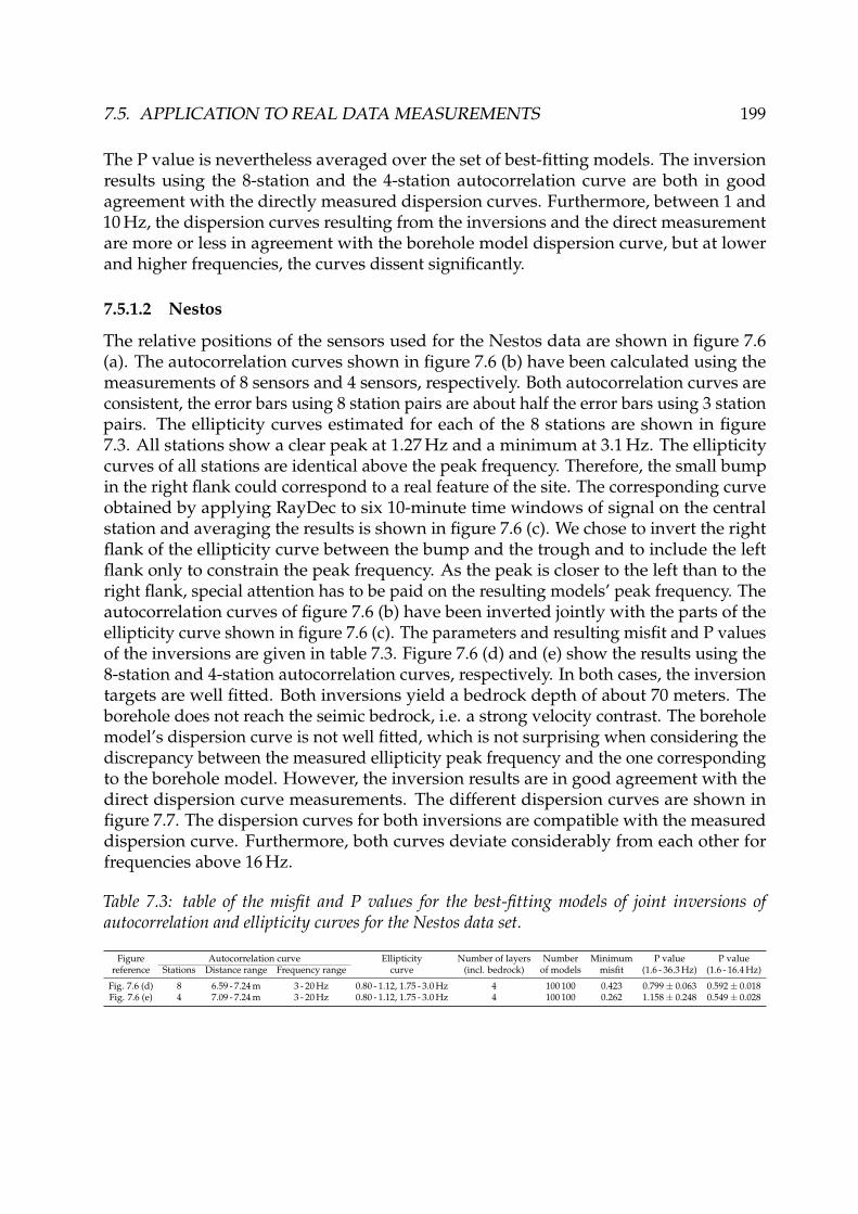
7.5. APPLICATION TO REAL DATA MEASUREMENTS 199

The P value is nevertheless averaged over the set of best-fitting models. The inversionresults using the 8-station and the 4-station autocorrelation curve are both in goodagreement with the directly measured dispersion curves. Furthermore, between 1 and10 Hz, the dispersion curves resulting from the inversions and the direct measurementare more or less in agreement with the borehole model dispersion curve, but at lowerand higher frequencies, the curves dissent significantly.

7.5.1.2 Nestos

The relative positions of the sensors used for the Nestos data are shown in figure 7.6(a). The autocorrelation curves shown in figure 7.6 (b) have been calculated using themeasurements of 8 sensors and 4 sensors, respectively. Both autocorrelation curves areconsistent, the error bars using 8 station pairs are about half the error bars using 3 stationpairs. The ellipticity curves estimated for each of the 8 stations are shown in figure7.3. All stations show a clear peak at 1.27 Hz and a minimum at 3.1 Hz. The ellipticitycurves of all stations are identical above the peak frequency. Therefore, the small bumpin the right flank could correspond to a real feature of the site. The corresponding curveobtained by applying RayDec to six 10-minute time windows of signal on the centralstation and averaging the results is shown in figure 7.6 (c). We chose to invert the rightflank of the ellipticity curve between the bump and the trough and to include the leftflank only to constrain the peak frequency. As the peak is closer to the left than to theright flank, special attention has to be paid on the resulting models’ peak frequency. Theautocorrelation curves of figure 7.6 (b) have been inverted jointly with the parts of theellipticity curve shown in figure 7.6 (c). The parameters and resulting misfit and P valuesof the inversions are given in table 7.3. Figure 7.6 (d) and (e) show the results using the8-station and 4-station autocorrelation curves, respectively. In both cases, the inversiontargets are well fitted. Both inversions yield a bedrock depth of about 70 meters. Theborehole does not reach the seimic bedrock, i.e. a strong velocity contrast. The boreholemodel’s dispersion curve is not well fitted, which is not surprising when considering thediscrepancy between the measured ellipticity peak frequency and the one correspondingto the borehole model. However, the inversion results are in good agreement with thedirect dispersion curve measurements. The different dispersion curves are shown infigure 7.7. The dispersion curves for both inversions are compatible with the measureddispersion curve. Furthermore, both curves deviate considerably from each other forfrequencies above 16 Hz.

Table 7.3: table of the misfit and P values for the best-fitting models of joint inversions ofautocorrelation and ellipticity curves for the Nestos data set.

Figure Autocorrelation curve Ellipticity Number of layers Number Minimum P value P valuereference Stations Distance range Frequency range curve (incl. bedrock) of models misfit (1.6 - 36.3 Hz) (1.6 - 16.4 Hz)

Fig. 7.6 (d) 8 6.59 - 7.24 m 3 - 20 Hz 0.80 - 1.12, 1.75 - 3.0 Hz 4 100 100 0.423 0.799± 0.063 0.592± 0.018Fig. 7.6 (e) 4 7.09 - 7.24 m 3 - 20 Hz 0.80 - 1.12, 1.75 - 3.0 Hz 4 100 100 0.262 1.158± 0.248 0.549± 0.028

200 CHAPTER 7. ELLIPTICITY INVERSION - REAL DATA

(a)

−10 −5 0 5

−5

0

5

Distance [m]

Dis

tanc

e [m

]

(b)

2 5 10 20

−0.5

0

0.5

1

Frequency [Hz]

Aut

ocor

rela

tion

ratio

8 stations4 stations (c)

0.5 1 2 5 10 20

0.5

1

2

3.5

5

10

Frequency [Hz]

Elli

ptic

ity

(d)

(e)

Figure 7.6: (a) Relative positions of the seismic sensors used for the study of Nestos. The stationpairs contributing to the spatial autocorrelation curves for the 8-station and the 4-station case arealso shown. (b) Spatial autocorrelation curves using 8 stations (8 station pairs, distances between6.59 and 7.24 m) and 4 stations (3 station pairs, distances between 7.09 and 7.24 m). The shadedareas indicate the measurement errors. The bold parts of the curves, delimited by the dashed lines,were used for the inversions. (c) Mean ellipticity and standard deviation obtained by cutting thesignal of the central station into six parts of 10 minutes each, applying RayDec and averaging theresults. The bold parts of the curve, delimited by the dashed lines, were used for the inversions.(d) and (e): Inversion results for joint inversions of the autocorrelation curve (left) and ellipticitycurve (center left) for the Nestos data set. The black dots indicate the data points used for theinversion and the black lines the curves for the borehole model. Dispersion curve (center, withdispersion curve data from array measurements) and shear wave velocity profiles (center right,zoom on the shallow layers on the right): (d) using the 8-station SPAC measurement (e) usingthe 4-station SPAC measurement.

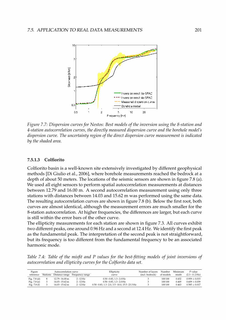
7.5. APPLICATION TO REAL DATA MEASUREMENTS 201

Figure 7.7: Dispersion curves for Nestos: Best models of the inversion using the 8-station and4-station autocorrelation curves, the directly measured dispersion curve and the borehole model’sdispersion curve. The uncertainty region of the direct dispersion curve measurement is indicatedby the shaded area.

7.5.1.3 Colfiorito

Colfiorito basin is a well-known site extensively investigated by different geophysicalmethods [Di Giulio et al., 2006], where borehole measurements reached the bedrock at adepth of about 50 meters. The locations of the seismic sensors are shown in figure 7.8 (a).We used all eight sensors to perform spatial autocorrelation measurements at distancesbetween 12.79 and 16.00 m. A second autocorrelation measurement using only threestations with distances between 14.03 and 15.62 m was performed using the same data.The resulting autocorrelation curves are shown in figure 7.8 (b). Below the first root, bothcurves are almost identical, although the measurement errors are much smaller for the8-station autocorrelation. At higher frequencies, the differences are larger, but each curveis still within the error bars of the other curve.The ellipticity measurements for each station are shown in figure 7.3. All curves exhibittwo different peaks, one around 0.96 Hz and a second at 12.4 Hz. We identify the first peakas the fundamental peak. The interpretation of the second peak is not straightforward,but its frequency is too different from the fundamental frequency to be an associatedharmonic mode.

Table 7.4: Table of the misfit and P values for the best-fitting models of joint inversions ofautocorrelation and ellipticity curves for the Colfiorito data set.

Figure Autocorrelation curve Ellipticity Number of layers Number Minimum P valuereference Stations Distance range Frequency range curve (incl. bedrock) of models misfit (2.3 - 11.2 Hz)

Fig. 7.8 (d) 8 12.79 - 16.00 m 2 - 12 Hz 0.50 - 0.83, 1.3 - 2.0 Hz 3 100 100 0.432 0.959± 0.015Fig. 7.8 (e) 3 14.03 - 15.62 m 2 - 12 Hz 0.50 - 0.83, 1.3 - 2.0 Hz 3 100 100 0.469 0.609± 0.039Fig. 7.8 (f) 3 14.03 - 15.62 m 2 - 12 Hz 0.50 - 0.83, 1.3 - 2.0, 3.5 - 10.0, 15.5 - 23.3 Hz 3 100 100 0.463 0.585± 0.017

202 CHAPTER 7. ELLIPTICITY INVERSION - REAL DATA

(a)

−20 −10 0 10 20

−10

0

10

Distance [m]

Dis

tanc

e [m

]

(b)

2 5 10 20

−0.5

0

0.5

1

Frequency [Hz]

Aut

ocor

rela

tion

ratio

8 stations4 stations

(c)

0.5 1 2 5 10 20

0.5

0.7

1

2

2.7

5

Frequency [Hz]

Elli

ptic

ity

(d)

(e)

(f)

Figure 7.8: (a) Relative positions of the seismic sensors used for the study of Colfiorito. The stationpairs contributing to the spatial autocorrelation curves for the 8-station and the 3-station caseare also shown. (b) Spatial autocorrelation curves using 8 stations (11 station pairs, distancesbetween 12.79 and 16.00 m) and 3 stations (3 station pairs, distances between 14.03 and 15.62 m).The shaded areas indicate the measurement errors. The bold parts of the curves, delimited by thedashed lines, were used for the inversions. (c) Mean ellipticity and standard deviation obtainedby cutting the signal of the central station into five parts of 9 minutes each, applying RayDec andaveraging the results. The bold parts of the curve, delimited by the dashed lines, were used for theinversions. For inversion (f), the dash-dotted part of the curve was also included in the inversion.(d) - (f): Inversion results for joint inversions of the autocorrelation curve (left) and ellipticitycurve (center left) for the Colfiorito data set. The black dots indicate the data points used for theinversion and the black lines the curves for the borehole model. Dispersion curve (center, withdispersion curve data from array measurements) and shear wave velocity profiles (center right,zoom on the shallow layers on the right): (d) using the 8-station SPAC measurement, (e) usingthe 3-station SPAC measurement, (f) using the 3-station SPAC measurement and including thesecond ellipticity peak.

7.5. APPLICATION TO REAL DATA MEASUREMENTS 203

Figure 7.9: Dispersion curves for Colfiorito: Best models of the inversion using the 8-station and3-station autocorrelation curves, the directly measured dispersion curve and the borehole model’sdispersion curve. The uncertainty region of the direct dispersion curve measurement is indicatedby the shaded area.

Therefore, we suggest that it is related to a small-scale resonance of superficial layers[Guéguen et al., 1998]. Figure 7.8 (c) shows the mean of the ellipticities obtained bycutting the signal of the central station into five pieces of 9 minutes each, applyingRayDec to them and averaging the results. The bold parts were used for the inversions.As the first peak is smaller than 3, we omitted ellipticity values above 2.7 Hz, in orderto allow for soil models with a singular peak. Here again, the left flank of the first peakserves to constrain the peak frequency only. Ellipticity values below 0.7 were omitted aswell, in order to leave the ellipticities around the trough unconstrained. For the inversionincluding the right peak, we used the same threshold values for both peaks.The given curves were inverted for models consisting of two homogeneous layers over ahomogeneous half-space. As this parameterization succeeds in retrieving a soil structureexplaining the measurements, we did not search for more complex parameterizations.The parameters and resulting misfit and P values of the inversions are given in table 7.4.In figures 7.8 (d) and (e), only the first peak has been inverted using the 8-station and the3-station autocorrelation curve, respectively. Both inversions give almost identical results.The respective autocorrelation and ellipticity curves are well fitted, the inversions yielda bedrock depth of about 42 meters. The resulting dispersion curves are in agreementwith the direct dispersion curve measurement. The 3-station inversion yields a better Pvalue than the 8-station inversion. Both the ellipticity measurement and the inversionresults are in contradiction with the borehole model. In figure 7.9, the dispersion curvesresulting from the inversion are compared to the borehole model’s and the directlymeasured curves.

204 CHAPTER 7. ELLIPTICITY INVERSION - REAL DATA

The indetermination of the resulting ellipticity curves at higher frequencies suggestedthat including the second ellipticity peak might improve the inversion. The resultinginversion obtained by using the second peak and attributing it to the fundamental modeare shown in figure 7.8 (f) for the 3-station autocorrelation curve only. The autocorrelationand ellipticity curves are still well fitted. The resulting dispersion curve exhibits apractically identical P value than without including the second peak. In figure 7.9,the inclusion of the second peak leaves the dispersion curve unchanged below 12 Hz,but changes it drastically above. The inversion algorithm models the second peak byintroducing a large velocity contrast between the first and the second layer. For thebest-fitting model, this leads to a first layer which is 75 cm thick with a velocity of40 m/s. The deeper layers are not affected by the second ellipticity peak. Finally, allinversions yield models which agree with the direct dispersion curve measurements.Including the second ellipticity peak does not significantly improve the inversion resultcompared with the direct dispersion curve measurements. This result is compatiblewith the presence of a very thin and very slow superficial layer, but as the inversionwithout the second peak yields comparable results without assuming such a layer, thishypothesis can neither be proven nor refuted. However, the attribution of the secondpeak to the fundamental Rayleigh wave mode would require that no higher modeswhich would alter the measurement were present in the wave field at all. AdditionalMASW measurements at high frequencies could help in identifying the nature of thesecond ellipticity peak.

7.5.2 Sites without clear ellipticity peak

7.5.2.1 Aigio

At Aigio, the array layout of the smallest ring was not adapted for small-scale spatialautocorrelation measurements and the next ring had a diameter of 30 meters. As wewant to show the possibility to retrieve the soil structure by small scale measurements,we decided to use the dispersion curve obtained by MASW measurements instead. Thisdispersion curve is shown in figure 7.10 (a). As the part of the curve between 12 and15 Hz is quite unstable, we use the curve between 15 and 28 Hz only. The ellipticity curveshown in figure 7.10 (b) was measured by the seismic station which was closest to theMASW profile. It is the mean curve for six 10-minute time windows of seismic noiserecordings. Calculating the apparent damping of the signal at 1.45 Hz identified theartificial origin of this peak. Therefore, the fundamental peak is the broad second peakwith an amplitude of 2 around 5 Hz. As the peak is broad, the complete peak between3.4 and 10.5 Hz was inverted.

Table 7.5: Table of the misfit and P values for the best-fitting models of joint inversions ofautocorrelation and ellipticity curves for the Aigio data set.

Figure Dispersion Ellipticity Number of layers Number Minimum P valuereference curve curve (incl. bedrock) of models misfit (7.3 - 28.5 Hz)

Fig. 7.10 (d) 15 - 28 Hz 3.4 - 10.5 Hz 4 100 100 0.144 0.506± 0.014

7.5. APPLICATION TO REAL DATA MEASUREMENTS 205

The high frequency of the ellipticity peak justifies the use of the high-frequency dispersioncurve above 15 Hz.The misfit and P values of the joint inversion of the dispersion and ellipticity data aregiven in table 7.5, the inversion results are shown in figure 7.10. Models consistingof three homogeneous layers overlying a half-space were necessary to correctly fit themeasurements. The inversion targets are well fitted, the dispersion curve disagreeswith the borehole model’s curve below 15 Hz. The directly measured dispersion curvewas obtained between 7.3 and 28.5 Hz. In this range, the curve is in good agreementwith the inversion result. Figure 7.10 (c) shows a comparison of the directly measured,borehole model and inverted dispersion curves. The shear wave velocity profiles matchthe borehole model quite well, except for the layer boundary which is given at 20 m bythe borehole and found at about 42 m by our inversions.

(a)

10 12 15 20 302

2.2

2.4

2.6

2.8

3

Frequency [Hz]

Slo

wne

ss [s

/km

]

(b)

1 2 5 10 20

0.5

1

2

3

Frequency [Hz]

Elli

ptic

ity

(c)

(d)

Figure 7.10: (a) Dispersion curve obtained by MASW measurements. The shaded area indicatesthe measurement errors. The bold part of the curve, delimited by the dashed lines, was usedfor the inversion. (b) Mean ellipticity and standard deviation obtained by cutting the signal ofstation next to the MASW measurements into six parts of 10 minutes each, applying RayDecand averaging the results. The shaded areas indicate the measurement errors. The bold part of thecurve, delimited by the dashed lines, was used for the inversion. (c) Dispersion curves for Aigio:Best models of the inversion, the directly measured dispersion curve and the borehole model’sdispersion curve. The uncertainty region of the direct dispersion curve measurement is indicatedby the shaded area. (d) Inversion results for joint inversions of the ellipticity curve (left, with datapoints) and dispersion curve (center left: data points with borehole model, center: with dispersioncurve data from array measurements) for the Aigio data set. The resulting shear wave velocityprofiles are shown on the right (center right: velocity profiles, right: zoom on the superficial 40meters). The black lines the curves for the borehole model.

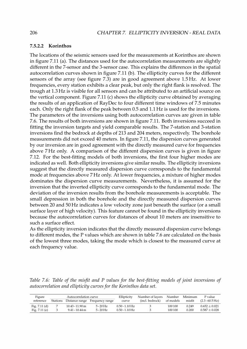
206 CHAPTER 7. ELLIPTICITY INVERSION - REAL DATA

7.5.2.2 Korinthos

The locations of the seismic sensors used for the measurements at Korinthos are shownin figure 7.11 (a). The distances used for the autocorrelation measurements are slightlydifferent in the 7-sensor and the 3-sensor case. This explains the differences in the spatialautocorrelation curves shown in figure 7.11 (b). The ellipticity curves for the differentsensors of the array (see figure 7.3) are in good agreement above 1.5 Hz. At lowerfrequencies, every station exhibits a clear peak, but only the right flank is resolved. Thetrough at 1.3 Hz is visible for all sensors and can be attributed to an artificial source onthe vertical component. Figure 7.11 (c) shows the ellipticity curve obtained by averagingthe results of an application of RayDec to four different time windows of 7.5 minuteseach. Only the right flank of the peak between 0.5 and 1.1 Hz is used for the inversions.The parameters of the inversions using both autocorrelation curves are given in table7.6. The results of both inversions are shown in figure 7.11. Both inversions succeed infitting the inversion targets and yield comparable results. The 7-station and 3-stationinversions find the bedrock at depths of 213 and 204 meters, respectively. The boreholemeasurements did not exceed 40 meters. In figure 7.11, the dispersion curves generatedby our inversion are in good agreement with the directly measured curve for frequenciesabove 7 Hz only. A comparison of the different dispersion curves is given in figure7.12. For the best-fitting models of both inversions, the first four higher modes areindicated as well. Both ellipticity inversions give similar results. The ellipticity inversionssuggest that the directly measured dispersion curve corresponds to the fundamentalmode at frequencies above 7 Hz only. At lower frequencies, a mixture of higher modesdominates the dispersion curve measurements. Nevertheless, it is assumed for theinversion that the inverted ellipticity curve corresponds to the fundamental mode. Thedeviation of the inversion results from the borehole measurements is acceptable. Thesmall depression in both the borehole and the directly measured dispersion curvesbetween 20 and 50 Hz indicates a low velocity zone just beneath the surface (or a smallsurface layer of high velocity). This feature cannot be found in the ellipticity inversionsbecause the autocorrelation curves for distances of about 10 meters are insensitive tosuch a surface effect.As the ellipticity inversion indicates that the directly measured dispersion curve belongsto different modes, the P values which are shown in table 7.6 are calculated on the basisof the lowest three modes, taking the mode which is closest to the measured curve ateach frequency value.

Table 7.6: Table of the misfit and P values for the best-fitting models of joint inversions ofautocorrelation and ellipticity curves for the Korinthos data set.

Figure Autocorrelation curve Ellipticity Number of layers Number Minimum P valuereference Stations Distance range Frequency range curve (incl. bedrock) of models misfit (2.3 - 60.5 Hz)

Fig. 7.11 (d) 7 10.43 - 11.90 m 5 - 20 Hz 0.50 - 1.10 Hz 3 100 100 0.249 0.652± 0.021Fig. 7.11 (e) 3 9.41 - 10.44 m 5 - 20 Hz 0.50 - 1.10 Hz 3 100 100 0.200 0.587± 0.028

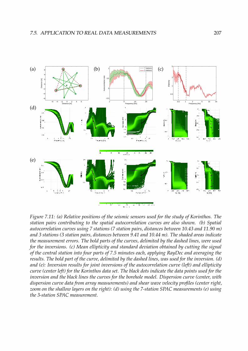
7.5. APPLICATION TO REAL DATA MEASUREMENTS 207

(a)

−6 −4 −2 0 2 4 6

−6

−4

−2

0

2

4

6

Distance [m]

Dis

tanc

e [m

]

(b)

2 5 10 20

−0.5

0

0.5

1

Frequency [Hz]A

utoc

orre

latio

n ra

tio

7 stations3 stations (c)

0.5 1 2 5 10 20

0.5

1

2

5

Frequency [Hz]

Elli

ptic

ity

(d)

(e)

Figure 7.11: (a) Relative positions of the seismic sensors used for the study of Korinthos. Thestation pairs contributing to the spatial autocorrelation curves are also shown. (b) Spatialautocorrelation curves using 7 stations (7 station pairs, distances between 10.43 and 11.90 m)and 3 stations (3 station pairs, distances between 9.41 and 10.44 m). The shaded areas indicatethe measurement errors. The bold parts of the curves, delimited by the dashed lines, were usedfor the inversions. (c) Mean ellipticity and standard deviation obtained by cutting the signalof the central station into four parts of 7.5 minutes each, applying RayDec and averaging theresults. The bold part of the curve, delimited by the dashed lines, was used for the inversion. (d)and (e): Inversion results for joint inversions of the autocorrelation curve (left) and ellipticitycurve (center left) for the Korinthos data set. The black dots indicate the data points used for theinversion and the black lines the curves for the borehole model. Dispersion curve (center, withdispersion curve data from array measurements) and shear wave velocity profiles (center right,zoom on the shallow layers on the right): (d) using the 7-station SPAC measurements (e) usingthe 3-station SPAC measurement.

208 CHAPTER 7. ELLIPTICITY INVERSION - REAL DATA

Figure 7.12: Dispersion curves for Korinthos: Best models of the inversion using the 8-stationand 3-station autocorrelation curves compared to the directly measured dispersion curve andthe borehole model’s dispersion curve. The uncertainty region of the direct dispersion curvemeasurement is indicated by the shaded area.

7.5. APPLICATION TO REAL DATA MEASUREMENTS 209

7.5.3 Inversion results for the other sites

Figure 7.13: Overview of the dispersion curves for the sites which are not treated in detail: Theresults for the best models resulting from joint inversions of ellipticity and autocorrelation curvesare compared with the dispersion curves obtained by direct measurements and the reference curves.

In the appendix, the inversions for the nine remaining sites are shown in detail. Figure7.13 compares the dispersion curves of the best-fitting models with the borehole modeldispersion curve as well as the direct dispersion curve measurements. The parametersof the respective inversions, among them the P values, are given in table 7.7. Except forForlì, P values below 1 could be achieved for all sites. For the sites of Buia, Knidi, Norciaand Sakarya, this can only be achieved by excluding areas of high frequency (above20 Hz, see table 7.7 for details) from the comparison. These frequencies are constrainedby the very superficial layers only, which are not well constrained by the data used forthe inversion. An autocorrelation curve which has its first root around 10 Hz does notinclude sufficient information on the shallowest layers. By including higher frequencymeasurements, e.g. MASW, in the inversion, these superficial layers could be constrainedin a better way.

210 CHAPTER 7. ELLIPTICITY INVERSION - REAL DATA

The ellipticity and autocorrelation measurements used for the inversions presented hereare not defined in that frequency range and therefore do not constrain the very superficiallayers. Consequently, it cannot be expected that our inversions fit the dispersion curvemeasurements at high frequencies and this part should not be compared. When neglect-ing high frequencies, for Benevento, Buia, Norcia, Sakarya and Sturno, a good agreementbetween the inversions and the direct measurements is given over the whole frequencyrange. For Bolu and Düzce, the fundamental mode resulting from the inversions andthe direct measurements diverge at frequencies below 5 Hz. However, looking at thehigher modes of the best model suggests that the direct measurement at these frequenciescorresponds to the first harmonic mode rather than to the fundamental one. In this way,the inversion of ellipticity curves can help to determine the modal nature of a measureddispersion curve.For Knidi, a comparison of the ellipticities of the individual sensors (see figure 7.3) al-ready indicated that the site is quite inhomogeneous and that a special attention has to bepaid for the inversion of ellipticity data. In fact, none of the stations of the smallest arrayshows a clear ellipticity peak, whereas the station near the borehole (which is locatedabout 40 meters west of the array) exhibits a clear peak. Consequently, the inversionresults are different depending on which ellipticity curve is used. The inversion of theellipticity of the station near the borehole is in better agreement with the dispersion curvethan the inversion using the ellipticity of the central station of the array (the autocorrela-tion information used in both inversions are identical). This could indicate that the deepstructure of the soil is different below the smallest array and that the soil structure atthe borehole is closer to the large-scale soil structure which is measured by the seismicarrays (the radius of the largest array measuring up to 140 meters).

Table 7.7: Table of the misfit and P values for the best-fitting models of joint inversions ofautocorrelation and ellipticity curves for the sites which are not shown in detail.

Site Autocorrelation curve Ellipticity Number Number Minimum P valueStations Distance range Frequency range curve of layers of models misfit Frequency range value

Benevento 6 7.14 - 9.48 m 6 - 25 Hz 2.0 - 19.1 Hz 3 100 100 0.386 1.7 - 26.4 Hz 0.696± 0.093

Bolu 8 7.56 - 9.29 m 3 - 20 Hz 0.4 - 4.0 Hz 4 100 100 0.247 1.7 - 30.3 Hz 0.691± 0.173

5.3 - 24.5 Hz 1.300± 0.008Buia 6 9.32 - 11.50 m 6 - 20 Hz 0.6 - 10.0 Hz 4 100 100 0.3185.3 - 20.4 Hz 0.631± 0.013

Düzce 7 8.01 - 8.83 m 6 - 20 Hz 0.5 - 2.7 Hz 4 100 100 0.406 1.7 - 40.0 Hz 0.537± 0.035

Forlì 7 7.41 - 9.35 m 3 - 20 Hz 0.7 - 10.0 Hz 3 100 100 0.415 3.1 - 31.9 Hz 1.173± 0.032

5.0 - 11.6 Hz 3.1 - 44.6 Hz 2.130± 0.044(central station)

3 100 100 0.2843.1 - 29.9 Hz 2.232± 0.044

Knidi 7 8.56 - 10.37 m 10 - 30 Hz6.4 - 11.6 Hz 3.1 - 44.6 Hz 1.198± 0.060

(station near borehole)3 100 100 0.420

3.1 - 29.9 Hz 0.508± 0.014

2.1 - 42.5 Hz 1.048± 0.098Norcia 7 8.67 - 9.97 m 8 - 35 Hz 1.0 - 20.1 Hz 3 100 100 0.5542.1 - 28.9 Hz 0.632± 0.164

2.8 - 36.3 Hz 1.064± 0.032Sakarya 7 11.89 - 13.67 m 8 - 25 Hz 3.0 - 5.4 Hz 3 100 100 0.4922.8 - 26.4 Hz 0.517± 0.021

Sturno 7 8.15 - 8.77 m 6 - 20 Hz 1.75 - 10.0 Hz 3 100 100 0.420 1.2 - 49.4 Hz 0.501± 0.021

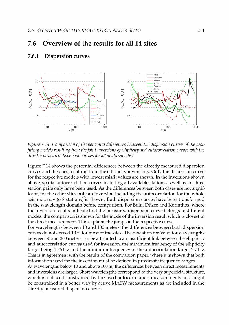
7.6. OVERVIEW OF THE RESULTS FOR ALL 14 SITES 211

7.6 Overview of the results for all 14 sites

7.6.1 Dispersion curves

10 100 1000

−20

0

20

λ [m]

(Vin

v/VD

C−

1) [%

]

Aigio

Benevento

Bolu

Buia

Colfiorito

Duzce

Forlı

10 100 1000

−20

0

20

λ [m]

(Vin

v/VD

C−

1) [%

]

Knidi

Korinthos

Nestos

Norcia

Sakarya

Sturno

Volvi

Figure 7.14: Comparison of the percental differences between the dispersion curves of the best-fitting models resulting from the joint inversions of ellipticity and autocorrelation curves with thedirectly measured dispersion curves for all analyzed sites.

Figure 7.14 shows the percental differences between the directly measured dispersioncurves and the ones resulting from the ellipticity inversions. Only the dispersion curvefor the respective models with lowest misfit values are shown. In the inversions shownabove, spatial autocorrelation curves including all available stations as well as for threestation pairs only have been used. As the differences between both cases are not signif-icant, for the other sites only an inversion including the autocorrelation for the wholeseismic array (6-8 stations) is shown. Both dispersion curves have been transformedin the wavelength domain before comparison. For Bolu, Düzce and Korinthos, wherethe inversion results indicate that the measured dispersion curve belongs to differentmodes, the comparison is shown for the mode of the inversion result which is closest tothe direct measurement. This explains the jumps in the respective curves.For wavelengths between 10 and 100 meters, the differences between both dispersioncurves do not exceed 10 % for most of the sites. The deviation for Volvi for wavelengthsbetween 50 and 300 meters can be attributed to an insufficient link between the ellipticityand autocorrelation curves used for inversion, the maximum frequency of the ellipticitytarget being 1.25 Hz and the minimum frequency of the autocorrelation target 2.7 Hz.This is in agreement with the results of the companion paper, where it is shown that bothinformation used for the inversion must be defined in proximate frequency ranges.At wavelengths below 10 and above 100 m, the differences between direct measurementsand inversions are larger. Short wavelengths correspond to the very superficial structure,which is not well constrained by the used autocorrelation measurements and mightbe constrained in a better way by active MASW measurements as are included in thedirectly measured dispersion curves.

212 CHAPTER 7. ELLIPTICITY INVERSION - REAL DATA

For large wavelengths, the bedrock velocity influences the dispersion curves. As hasbeen shown in the first paper on the theoretical aspects of ellipticity inversions, thisparameter is badly constrained by the ellipticity curve. A loss of agreement to the directmeasurements at these wavelengths is therefore not surprising.

7.6.2 Vs30 values

100 200 300 400 500 600 700 800100

200

300

400

500

600

700

Aigio

Benevento

Bolu

Buia

Colfiorito

DuzceForlı

Knidi

Korinthos

Nestos

Norcia

Sakarya

Sturno

Volvi

Vs30borehole

Vs3

0 inve

rsio

n

100 200 300 400 500 600 700100

200

300

400

500

600

700

Aigio

Benevento

Bolu

Buia

Colfiorito

Duzce

Forlı

Knidi

Korinthos

Nestos

Norcia

Sakarya

Sturno

Volvi

Vs30DC inversion

Vs3

0 Ell.

inve

rsio

n

Figure 7.15: Left: Comparison of the Vs30 values from borehole measurements (or referencemeasurements for Bolu, Düzce and Sakarya) with the values resulting from the joint inversionsof ellipticity and autocorrelation curves. The dotted lines indicate the limits of the EC8 classes.Right: Comparison of the Vs30 values obtained by inversion of a broad frequency-range dispersioncurve with the joint inversions of ellipticity and autocorrelation curves.

The Vs30 value indicates the mean shear wave velocity over the uppermost 30 meters.This value is used in the actual seismic codes for buildings. In the article on the theoreticalaspects of ellipticity inversion, it has been shown that the superficial layers are principallyconstrained by the autocorrelation curves. However, when measuring autocorrelationcurves, the ellipticity can be easily calculated using the same data without furthermeasurement efforts and be included in the inversion process. In this way, joint ellipticityand autocorrelation inversions represent an easier and cheaper way of measurementthan borehole measurements. In figure 7.15, the Vs30 values resulting from our ellipticityinversions are compared to the values obtained by borehole measurements (or referenceMASW measurements for Bolu, Düzce and Sakarya). For 9 of the 14 analyzed sites, bothvalues are in very good agreement. All the other sites are stiff or rock sites. At least forsoft sites, joint inversions involving ellipticity curves present a simple and cheap methodto characterize the soil structure.In figure 7.15, the Vs30 values resulting from our ellipticity inversions are also comparedto the Vs30 values which result from the inversion of broad-band dispersion curves [DiGiulio et al., 2010]. Except for some sites exhibiting a complicated soil structure, the Vs30values resulting from both inversions are in very good agreement.

7.7. CONCLUSION 213

7.7 Conclusion

In this article, it has been shown that joint inversions of ellipticity and spatial autocor-relation or dispersion curves yield soil structure models which are in good agreementwith direct dispersion curve measurements. Furthermore, using only a small number ofstations for the SPAC measurements yields results which are in complete agreement withmeasurements including more sensors. In this way, our method presents an easy andcheap way to investigate the soil structure. For 13 of the 14 investigated sites, P valuesbelow 1 can be found if high frequencies are disregarded. An inclusion of informationat high frequencies as obtained by MASW measurements could enhance the constraintof the shallowest structure. However, it can be disputed if the expected improvementsjustify the additional measurement effort. Nonetheless, the presented method is notcapable to determine the exact bedrock velocity.Furthermore, at some sites, the inversions can even help in identifying the fundamentaland harmonic Rayleigh wave modes in cases where the directly measured dispersioncurve, if regarded separately, could reasonably represent the fundamental mode overthe whole frequency range as well. For Buia, Düzce and Korinthos, the ellipticity curveinversions clearly suggest that, at low frequencies, the directly measured dispersioncurves are dominated by the first or second harmonic mode.Although the present study’s aim was not to determine Vs30 values, but to find thewhole soil structure, it yields very good agreements with borehole measurements formost of the sites. All sites with a worse consistency are stiff or rock sites. At least forsoft sites, the presented method can be very helpful for seismic hazard assessment. Asthe measurements can be performed quickly, a dense survey of a given area can beperformed in order to find small-scale irregularities.

Acknowledgments

We would like to thank all those who helped to perform the measurements:Mehmet Akif Alkan, Marios Anthimidis, Stéphane Drouet, Markus Gurk, Yıldız Iravul,Ioannis Kalogeras, Andreas Köhler, Armand Mariscal, Jean-Marc Nicole, Özgür TunaÖzmen, Carsten Riggelsen, Abdullah Sandıkkaya, Paula Teves-Costa, Bekir Tüzel, DanielVollmer and Ali Zeynel.

7.8. APPENDIX: INVERSION RESULTS FOR THE OTHER SITES IN DETAIL 215

7.8 Appendix:Inversion results for the other sites in detail

7.8.1 BeneventoThe Benevento measurements have been performed on a stiff site. The locations of theseismic sensors are shown in figure 7.16 (a). Six sensors forming eight station pairs havebeen used to calculate the autocorrelation curve (see figure 7.16 (b)). The ellipticity curve(figure 7.16 (c)) was obtained by using 55 minutes of seismic noise recordings of thecentral station (averaging five windows of eleven minutes). The peak at 10 Hz couldbe a singularity, but none of our inversions succeeded in fitting a singular peak to thispoint. Therefore, we take the peak as a flat peak and include it in the inversion processas a whole. In the frequency range between 2.0 and 19.1 Hz, which was used for theinversion, the ellipticity curves of the central station and the ring stations are in goodagreement.The parameters of the inversion are given in table 7.8, the results are shown in figure 7.16(e). The autocorrelation and ellipticity data are well fitted, the dispersion curve of theinversion is in qualitative agreement with the directly measured one (see figure 7.16 (d)).Both dispersion curves do not fit the borehole measurement.

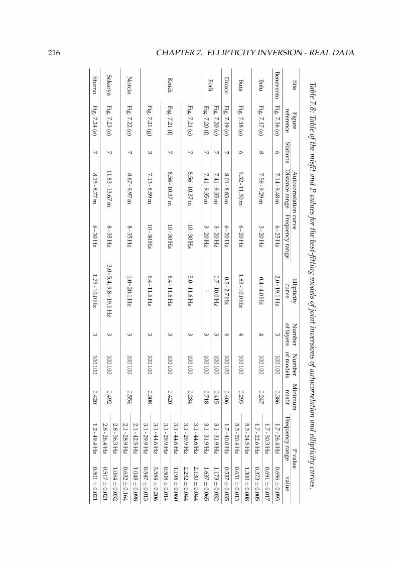
216 CHAPTER 7. ELLIPTICITY INVERSION - REAL DATA

Table7.8:Table

ofthem

isfitandP

valuesfor

thebest-fitting

models

ofjointinversionsofautocorrelation

andellipticity

curves.

SiteFigure

Autocorrelation

curveEllipticity

Num

berN

umber

Minim

umP

valuereference

StationsD

istancerange

Frequencyrange

curveoflayers

ofmodels

misfit

Frequencyrange

value

BeneventoFig.7.16

(e)6

7.14-9.48

m6

-25H

z2.0

-19.1H

z3

100100

0.3861.7

-26.4H

z0.696±

0.093

1.7-30.3

Hz

0.691±0.017

BoluFig.7.17

(e)8

7.56-9.29

m3

-20H

z0.4

-4.0H

z4

100100

0.2471.7

-22.6H

z0.373±

0.005

5.3-24.5

Hz

1.300±0.008

BuiaFig.7.18

(e)6

9.32-11.50

m6

-20H

z1.85

-10.0H

z4

100100

0.2935.3

-20.4H

z0.631±

0.013

Düzce

Fig.7.19(e)

78.01

-8.83m

6-20

Hz

0.5-2.7

Hz

4100

1000.406

1.7-40.0

Hz

0.537±0.035

Fig.7.20(e)

77.41

-9.35m

3-20

Hz

0.7-10.0

Hz

3100

1000.415

3.1-31.9

Hz

1.173±0.032

ForlìFig.7.20

(f)7

7.41-9.35

m3

-20H

z-

3100

1000.718

3.1-31.9

Hz

1.637±0.065

3.1-44.6

Hz

2.130±0.044

Fig.7.21(e)

78.56

-10.37m

10-30

Hz

5.0-11.6

Hz

3100

1000.284

3.1-29.9

Hz

2.232±0.044

3.1-44.6

Hz

1.198±0.060

Knidi

Fig.7.21(f)

78.56

-10.37m

10-30

Hz

6.4-11.6

Hz

3100

1000.420

3.1-29.9

Hz

0.508±0.014

3.1-44.6

Hz

3.584±0.206

Fig.7.21(g)

37.13

-8.59m

10-30

Hz

6.4-11.6

Hz

3100

1000.308

3.1-29.9

Hz

0.547±0.013

2.1-42.5

Hz

1.048±0.098

Norcia

Fig.7.22(e)

78.67

-9.97m

8-35

Hz

1.0-20.1

Hz

3100

1000.554

2.1-28.9

Hz

0.632±0.164

2.8-36.3

Hz

1.064±0.032

SakaryaFig.7.23

(e)7

11.83-13.67

m8

-35H

z3.0

-5.4,9.8-19.1

Hz

3100

1000.492

2.8-26.4

Hz

0.517±0.021

SturnoFig.7.24

(e)7

8.15-8.77

m6

-30H

z1.75

-10.0H

z3

100100

0.4201.2

-49.4H

z0.501±

0.021

7.8. APPENDIX: INVERSION RESULTS FOR THE OTHER SITES IN DETAIL 217

(a)

−4 −2 0 2 4

−2

0

2

4

Distance [m]

Dis

tanc

e [m

]

(b)

2 5 10 20

−0.5

0

0.5

1

Frequency [Hz]

Aut

ocor

rela

tion

ratio

(c)

0.5 1 2 5 10 20

0.5

1

2

3

Frequency [Hz]

Elli

ptic

ity

(d)

(e)

Figure 7.16: (a) Relative positions of the seismic sensors used for the study of Benevento. Thestation pairs contributing to the spatial autocorrelation curve are also shown. (b) Spatial autocor-relation curve using 6 stations (8 station pairs, distances between 7.14 and 9.48 m). The shadedarea indicates the measurement errors. The bold part of the curve, delimited by the dashed lines,was used for the inversion. (c) Mean ellipticity and standard deviation obtained by cutting thesignal of the central station into five parts of 11 minutes each, applying RayDec and averagingthe results. The bold part of the curve, delimited by the dashed lines, was used for the inversion.(d) Dispersion curves: Best models of the inversion compared to the directly measured dispersioncurve and the borehole model’s dispersion curve. The incertainty region of the direct dispersioncurve measurement is indicated by the shaded area. (e) Inversion results for joint inversions of theautocorrelation curve (left) and ellipticity curve (center left) for the Benevento data set. The blackdots indicate the data points used for the inversion and the black lines the curves for the boreholemodel. Dispersion curve (center right, with dispersion curve data from array measurements) andshear wave velocity profiles (right).

218 CHAPTER 7. ELLIPTICITY INVERSION - REAL DATA

7.8.2 BoluThe layout of the array of seismic sensors used for the Bolu measurements is shown infigure 7.17 (a). Six station pairs involving eight seismic sensors were used to calculatethe autocorrelation curve of figure 7.17 (b). The ellipticity curves of the different sensorsshown in figure 7.3 are in good mutual agreement below 5 Hz. The ellipticity curveshown in figure 7.17 (c) results from an averaging of four ten-minute windows of seismicnoise signals of the central station. As the ellipticity curve is rather flat, the bumpbetween 0.4 and 4.0 Hz is used for the inversion.Both the autocorrelation and the ellipticity curve are well fitted by the inversion (seetable 7.8 for the parameters and figure 7.17 (e) for the inversion results). The dispersioncurves obtained by the inversion are compatible with the directly measured ones atleast between 5 and 20 Hz, as can be seen in figure 7.17 (d). The higher modes forthe best inversion model are shown as well. At frequencies below 3 Hz, the inversionsuggests that the directly measured dispersion curve corresponds to the first harmonicmode rather than the fundamental one. According to this interpretation, the measureddispersion curve between 3 and 8 Hz would correspond to a mixture of the two lowestmodes. The calculation of the P value in table 7.8 is based on both modes, whichever isclosest to the data.

7.8. APPENDIX: INVERSION RESULTS FOR THE OTHER SITES IN DETAIL 219

(a)

−5 0 5 10

−5

0

5

Distance [m]

Dis

tanc

e [m

]

(b)

2 5 10 20

−0.5

0

0.5

1

Frequency [Hz]

Aut

ocor

rela

tion

ratio

(c)

0.5 1 2 5 10 20

0.5

1

2

3

Frequency [Hz]

Elli

ptic

ity

(d)

(e)

Figure 7.17: (a) Relative positions of the seismic sensors used for the study of Bolu. The stationpairs contributing to the spatial autocorrelation curve are also shown. (b) Spatial autocorrelationcurve using 8 stations (6 station pairs, distances between 7.56 and 9.29 m). The shaded areaindicates the measurement errors. The bold part of the curve, delimited by the dashed lines, wasused for the inversion. (c) Mean ellipticity and standard deviation obtained by cutting the signalof the central station into four parts of 10 minutes each, applying RayDec and averaging theresults. The bold part of the curve, delimited by the dashed lines, was used for the inversion. (d)Dispersion curves: Best models of the inversion compared to the directly measured dispersioncurve and the reference model’s dispersion curve. The uncertainty region of the direct dispersioncurve measurement is indicated by the shaded area. (e) Inversion results for joint inversions ofthe autocorrelation curve (left) and ellipticity curve (center left) for the Bolu data set. The blackdots indicate the data points used for the inversion and the black lines the curves for the referencemodel. Dispersion curve (center, with dispersion curve data from array measurements) and shearwave velocity profiles (center right, zoom on the shallow layers on the right).

220 CHAPTER 7. ELLIPTICITY INVERSION - REAL DATA

7.8.3 BuiaFor the Buia measurements, the autocorrelation curve (figure 7.18 (b)) was obtained byusing the seven station pairs indicated in figure 7.18 (a). The ellipticity curves of all ofthese stations show an artificial peak at 1.45 Hz (see figure 7.3). The second peak at 6.8 Hzis, despite its shape, not artificial, therefore we identify it as a soil feature and invert theellipticity curve for the central station between 1.85 and 10.0 Hz (see figure 7.18 (c)).For the inversion, the parameters are given in table 7.8 and the results in figure 7.18 (e).The autocorrelation and ellipticity data are well fitted. The dispersion curve resulting ofthe inversion is in good agreement with the direct measurement for frequencies below20 Hz (see figure 7.18 (d)). Above that frequency, the inversion results are not wellconstrained as the autocorrelation curve carries information between 6 and 20 Hz only.

7.8. APPENDIX: INVERSION RESULTS FOR THE OTHER SITES IN DETAIL 221

(a)

−6 −4 −2 0 2 4 6

−6

−4

−2

0

2

4

6

Distance [m]

Dis

tanc

e [m

]

(b)

2 5 10 20

−0.5

0

0.5

1

Frequency [Hz]

Aut

ocor

rela

tion

ratio

(c)

0.5 1 2 5 10 20

1

2

5

Frequency [Hz]

Elli

ptic

ity

(d)

(e)

Figure 7.18: (a) Relative positions of the seismic sensors used for the study of Buia. The stationpairs contributing to the spatial autocorrelation curves are also shown. (b) Spatial autocorrelationcurve using 6 stations (7 station pairs, distances between 9.32 and 11.50 m). The shaded areaindicates the measurement errors. The bold part of the curve, delimited by the dashed lines, wasused for the inversion. (c) Mean ellipticity and standard deviation obtained by cutting the signalof the central station into six parts of 10 minutes each, applying RayDec and averaging theresults. The bold part of the curve, delimited by the dashed lines, was used for the inversion. (d)Dispersion curves: Best models of the inversion compared to the directly measured dispersioncurve and the borehole model’s dispersion curve. The uncertainty region of the direct dispersioncurve measurement is indicated by the shaded area. (e) Inversion results for joint inversions ofthe autocorrelation curve (left) and ellipticity curve (center left) for the Buia data set. The blackdots indicate the data points used for the inversion and the black lines the curves for the boreholemodel. Dispersion curve (center right, with dispersion curve data from array measurements) andshear wave velocity profiles (right).

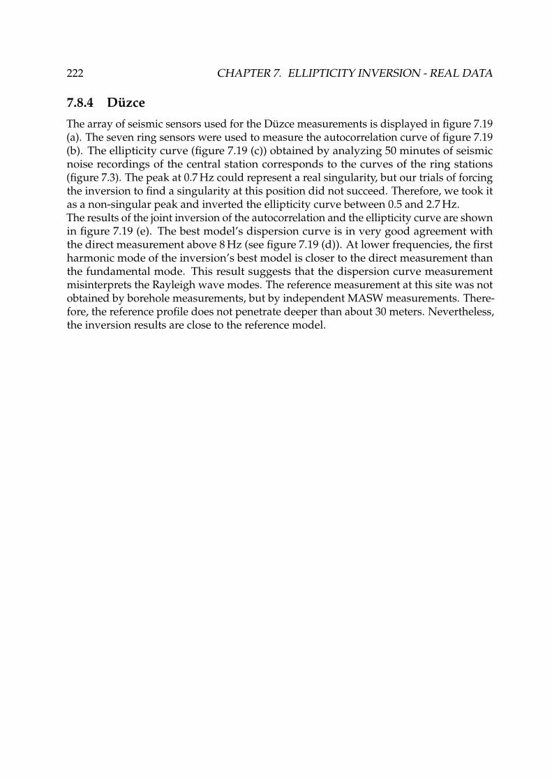
222 CHAPTER 7. ELLIPTICITY INVERSION - REAL DATA

7.8.4 DüzceThe array of seismic sensors used for the Düzce measurements is displayed in figure 7.19(a). The seven ring sensors were used to measure the autocorrelation curve of figure 7.19(b). The ellipticity curve (figure 7.19 (c)) obtained by analyzing 50 minutes of seismicnoise recordings of the central station corresponds to the curves of the ring stations(figure 7.3). The peak at 0.7 Hz could represent a real singularity, but our trials of forcingthe inversion to find a singularity at this position did not succeed. Therefore, we took itas a non-singular peak and inverted the ellipticity curve between 0.5 and 2.7 Hz.The results of the joint inversion of the autocorrelation and the ellipticity curve are shownin figure 7.19 (e). The best model’s dispersion curve is in very good agreement withthe direct measurement above 8 Hz (see figure 7.19 (d)). At lower frequencies, the firstharmonic mode of the inversion’s best model is closer to the direct measurement thanthe fundamental mode. This result suggests that the dispersion curve measurementmisinterprets the Rayleigh wave modes. The reference measurement at this site was notobtained by borehole measurements, but by independent MASW measurements. There-fore, the reference profile does not penetrate deeper than about 30 meters. Nevertheless,the inversion results are close to the reference model.

7.8. APPENDIX: INVERSION RESULTS FOR THE OTHER SITES IN DETAIL 223

(a)

−6 −4 −2 0 2 4 6

−4

−2

0

2

4

6

Distance [m]

Dis

tanc

e [m

]

(b)

2 5 10 20

−0.5

0

0.5

1

Frequency [Hz]

Aut

ocor

rela

tion

ratio

(c)

0.5 1 2 5 10 200.5

1

2

5

Frequency [Hz]

Elli

ptic

ity

(d)

(e)

Figure 7.19: (a) Relative positions of the seismic sensors used for the study of Düzce. The stationpairs contributing to the spatial autocorrelation curve are also shown. (b) Spatial autocorrelationcurve using 7 stations (7 station pairs, distances between 8.01 and 8.83 m). The shaded areaindicates the measurement errors. The bold part of the curve, delimited by the dashed lines, wasused for the inversion. (c) Mean ellipticity and standard deviation obtained by cutting the signalof the central station into five parts of 10 minutes each, applying RayDec and averaging theresults. The bold part of the curve, delimited by the dashed lines, was used for the inversion. (d)Dispersion curves: Best models of the inversion compared to the directly measured dispersioncurve and the reference model’s dispersion curve. The uncertainty region of the direct dispersioncurve measurement is indicated by the shaded area. (e) Inversion results for joint inversions ofthe autocorrelation curve (7-station measurement, left) and ellipticity curve (center left) for theDüzce data set. The black dots indicate the data points used for the inversion and the black linesthe curves for the reference model. Dispersion curve (center, with dispersion curve data fromarray measurements) and shear wave velocity profiles (center right, zoom on the shallow layerson the right).

224 CHAPTER 7. ELLIPTICITY INVERSION - REAL DATA

7.8.5 ForlìAt Forlì, all stations (see figure 7.20 (a) for the locations) exhibit a flat ellipticity curvewith values hardly exceeding 1. Nevertheless, the ellipticity curve has a bump around2 Hz. We invert the ellipticity curve calculated for 45 minutes of seismic noise for thecentral station of the array between 0.7 and 10.0 Hz (see figure 7.20 (c)) jointly with theautocorrelation curve calculated by using nine station pairs of the seven ring stations(figure 7.20 (b)).As the autocorrelation curve used for the inversion is defined in the same frequencyregion (3 - 20 Hz) as the ellipticity curve, one could argue that the both informations areredundant. Therefore, we performed a second inversion of the autocorrelation curveonly. The parameters of both inversions are given in table 7.8 and the respective resultsin figure 7.20 (e) and (f).It can be seen that the inclusion of the ellipticity information improves the inversionresult by further constraining the possible solutions and acting particularly on the deeperlayers. In figure 7.20 (d), the dispersion curves of the best models of both inversionsare compared to the measured dispersion curve. Above 5 Hz, both inversions’ resultsare identical. At lower frequencies, the inversion including the ellipticity data is veryclose to the measured dispersion curve, whereas the autocorrelation inversion deviatesconsiderably. This effect is reflected in the P values as well. At frequencies above 15 Hz,both inversions are in contradiction with the dispersion curve measurement, certainlybecause the autocorrelation curve does not sufficiently constrain the very superficiallayers. Therefore, the P values of both inversions do not go below 1.

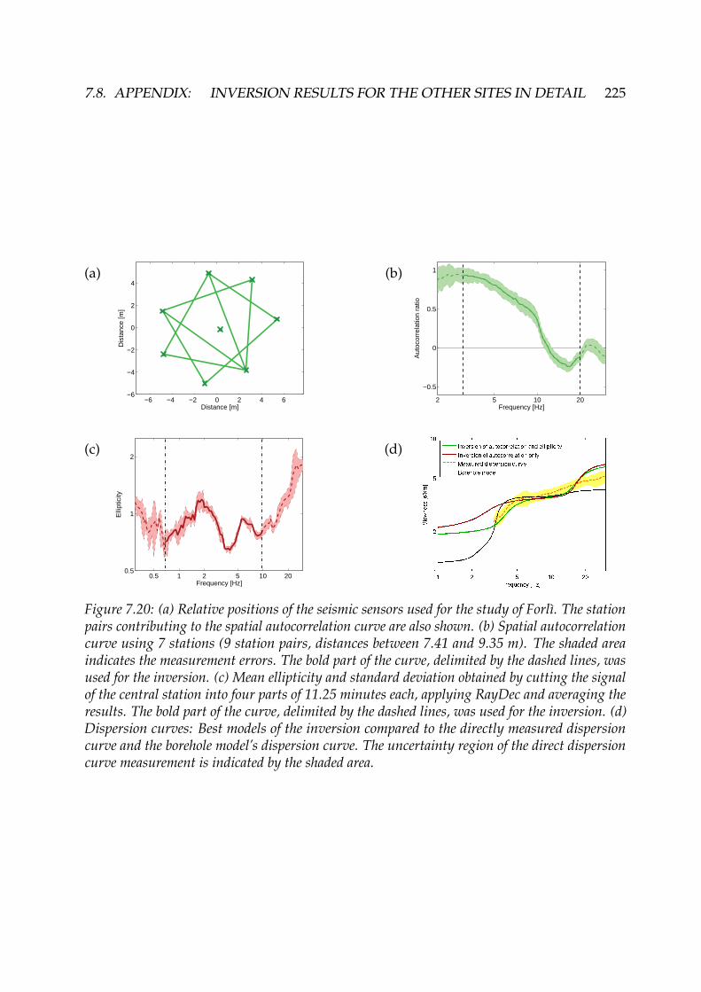
7.8. APPENDIX: INVERSION RESULTS FOR THE OTHER SITES IN DETAIL 225

(a)

−6 −4 −2 0 2 4 6−6

−4

−2

0

2

4

Distance [m]

Dis

tanc

e [m

]

(b)

2 5 10 20

−0.5

0

0.5

1

Frequency [Hz]A

utoc

orre

latio

n ra

tio

(c)

0.5 1 2 5 10 200.5

1

2

Frequency [Hz]

Elli

ptic

ity

(d)

Figure 7.20: (a) Relative positions of the seismic sensors used for the study of Forlì. The stationpairs contributing to the spatial autocorrelation curve are also shown. (b) Spatial autocorrelationcurve using 7 stations (9 station pairs, distances between 7.41 and 9.35 m). The shaded areaindicates the measurement errors. The bold part of the curve, delimited by the dashed lines, wasused for the inversion. (c) Mean ellipticity and standard deviation obtained by cutting the signalof the central station into four parts of 11.25 minutes each, applying RayDec and averaging theresults. The bold part of the curve, delimited by the dashed lines, was used for the inversion. (d)Dispersion curves: Best models of the inversion compared to the directly measured dispersioncurve and the borehole model’s dispersion curve. The uncertainty region of the direct dispersioncurve measurement is indicated by the shaded area.

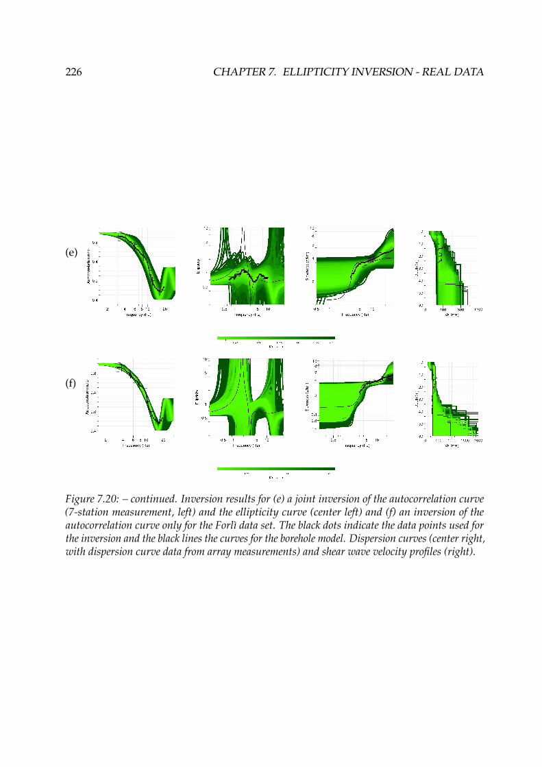
226 CHAPTER 7. ELLIPTICITY INVERSION - REAL DATA

(e)

(f)

Figure 7.20: – continued. Inversion results for (e) a joint inversion of the autocorrelation curve(7-station measurement, left) and the ellipticity curve (center left) and (f) an inversion of theautocorrelation curve only for the Forlì data set. The black dots indicate the data points used forthe inversion and the black lines the curves for the borehole model. Dispersion curves (center right,with dispersion curve data from array measurements) and shear wave velocity profiles (right).

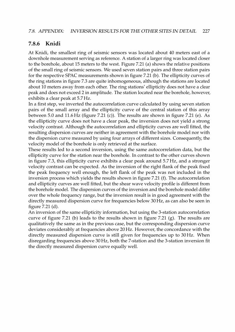
7.8. APPENDIX: INVERSION RESULTS FOR THE OTHER SITES IN DETAIL 227

7.8.6 KnidiAt Knidi, the smallest ring of seismic sensors was located about 40 meters east of adownhole measurement serving as reference. A station of a larger ring was located closerto the borehole, about 15 meters to the west. Figure 7.21 (a) shows the relative positionsof the small ring of seismic sensors. We used seven station pairs and three station pairsfor the respective SPAC measurements shown in figure 7.21 (b). The ellipticity curves ofthe ring stations in figure 7.3 are quite inhomogeneous, although the stations are locatedabout 10 meters away from each other. The ring stations’ ellipticity does not have a clearpeak and does not exceed 2 in amplitude. The station located near the borehole, however,exhibits a clear peak at 5.7 Hz.In a first step, we inverted the autocorrelation curve calculated by using seven stationpairs of the small array and the ellipticity curve of the central station of this arraybetween 5.0 and 11.6 Hz (figure 7.21 (c)). The results are shown in figure 7.21 (e). Asthe ellipticity curve does not have a clear peak, the inversion does not yield a strongvelocity contrast. Although the autocorrelation and ellipticity curves are well fitted, theresulting dispersion curves are neither in agreement with the borehole model nor withthe dispersion curve measured by using four arrays of different sizes. Consequently, thevelocity model of the borehole is only retrieved at the surface.These results led to a second inversion, using the same autocorrelation data, but theellipticity curve for the station near the borehole. In contrast to the other curves shownin figure 7.3, this ellipticity curve exhibits a clear peak around 5.7 Hz, and a strongervelocity contrast can be expected. As the inversion of the right flank of the peak fixedthe peak frequency well enough, the left flank of the peak was not included in theinversion process which yields the results shown in figure 7.21 (f). The autocorrelationand ellipticity curves are well fitted, but the shear wave velocity profile is different fromthe borehole model. The dispersion curves of the inversion and the borehole model differover the whole frequency range, but the inversion result is in good agreement with thedirectly measured dispersion curve for frequencies below 30 Hz, as can also be seen infigure 7.21 (d).An inversion of the same ellipticity information, but using the 3-station autocorrelationcurve of figure 7.21 (b) leads to the results shown in figure 7.21 (g). The results arequalitatively the same as in the previous case, but the corresponding dispersion curvedeviates considerably at frequencies above 20 Hz. However, the concordance with thedirectly measured dispersion curve is still given for frequencies up to 30 Hz. Whendisregarding frequencies above 30 Hz, both the 7-station and the 3-station inversion fitthe directly measured dispersion curve equally well.

228 CHAPTER 7. ELLIPTICITY INVERSION - REAL DATA

(a)

−6 −4 −2 0 2 4 6

−4

−2

0

2

4

6

Distance [m]

Dis

tanc

e [m

]

(b)

5 10 20

−0.5

0

0.5

1

Frequency [Hz]

Aut

ocor

rela

tion

ratio

7 stations3 stations

(c)

1 2 5 10 20

0.5

1

2

5

10

Frequency [Hz]

Elli

ptic

ity

Central stationnear borehole (d)

Figure 7.21: (a) Relative positions of the seismic sensors used for the study of Knidi. The stationpairs contributing to the spatial autocorrelation curves for the 7-station and the 3-station caseare also shown. The location of the borehole site 50 meters west of the array and of the stationnear the borehole (15 meters from the borehole) are not shown. (b) Spatial autocorrelation curvesusing 7 stations (7 station pairs, distances between 8.56 and 10.37 m) and 3 stations (3 stationpairs, distances between 7.13 and 8.59 m). The shaded areas indicate the measurement errors. Thebold parts of the curves, delimited by the dashed lines, were used for the inversion. The differentdistances of both measurements explain the shift between both curves. (c) Mean ellipticity andstandard deviation obtained by cutting the signal of the station near the borehole into four partsof 7.5 minutes each, applying RayDec and averaging the results. The bold parts of the curves,delimited by the dashed lines, were used for the inversions. (d) Dispersion curves for Knidi: Bestmodels of the inversion using the 7-station and 3-station autocorrelation curves compared to thedirectly measured dispersion curve and the borehole model’s dispersion curve. The uncertaintyregion of the direct dispersion curve measurement is indicated by the shaded area.

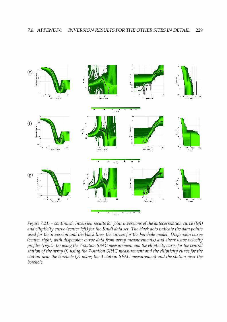
7.8. APPENDIX: INVERSION RESULTS FOR THE OTHER SITES IN DETAIL 229

(e)

(f)

(g)

Figure 7.21: – continued. Inversion results for joint inversions of the autocorrelation curve (left)and ellipticity curve (center left) for the Knidi data set. The black dots indicate the data pointsused for the inversion and the black lines the curves for the borehole model. Dispersion curve(center right, with dispersion curve data from array measurements) and shear wave velocityprofiles (right): (e) using the 7-station SPAC measurement and the ellipticity curve for the centralstation of the array (f) using the 7-station SPAC measurement and the ellipticity curve for thestation near the borehole (g) using the 3-station SPAC measurement and the station near theborehole.

230 CHAPTER 7. ELLIPTICITY INVERSION - REAL DATA

7.8.7 NorciaThe positions of the sensors of the seismic array used for the study of Norcia are given infigure 7.22 (a). The autocorrelation curve (figure 7.22 (b)) results from analyzing eightstation pairs using the ring stations. The different stations exhibit major differences inthe ellipticity curves below 1 Hz (figure 7.3). Around the peak frequency of 8 Hz, allstations exhibit virtually identical curves. As no inversion with an ellipticity singularityat that frequency could be found, we took the peak as a non-singular one. The ellipticitycurve in figure 7.22 (c) was obtained by analyzing 45 minutes of seismic noise recordedby the central station. A joint inversion of the autocorrelation and the ellipticity curvesyields the results shown in figure 7.22 (e). Although the ellipticity curve is not too wellfitted, the resulting dispersion curve (figure 7.22 (d)) is very close to the measured one,at least below 30 Hz.

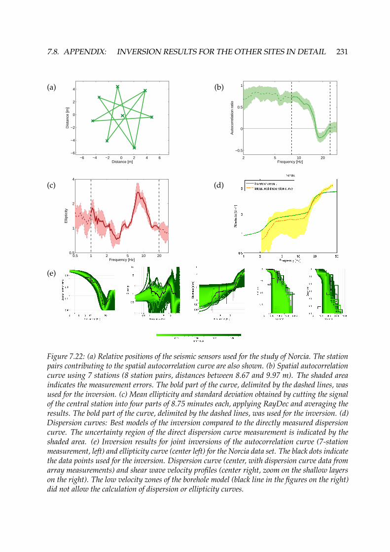
7.8. APPENDIX: INVERSION RESULTS FOR THE OTHER SITES IN DETAIL 231

(a)

−6 −4 −2 0 2 4 6−6

−4

−2

0

2

4

Distance [m]

Dis

tanc

e [m

]

(b)

2 5 10 20

−0.5

0

0.5

1

Frequency [Hz]

Aut

ocor

rela

tion

ratio

(c)

0.5 1 2 5 10 200.5

1

2

4

Frequency [Hz]

Elli

ptic

ity

(d)

(e)

Figure 7.22: (a) Relative positions of the seismic sensors used for the study of Norcia. The stationpairs contributing to the spatial autocorrelation curve are also shown. (b) Spatial autocorrelationcurve using 7 stations (8 station pairs, distances between 8.67 and 9.97 m). The shaded areaindicates the measurement errors. The bold part of the curve, delimited by the dashed lines, wasused for the inversion. (c) Mean ellipticity and standard deviation obtained by cutting the signalof the central station into four parts of 8.75 minutes each, applying RayDec and averaging theresults. The bold part of the curve, delimited by the dashed lines, was used for the inversion. (d)Dispersion curves: Best models of the inversion compared to the directly measured dispersioncurve. The uncertainty region of the direct dispersion curve measurement is indicated by theshaded area. (e) Inversion results for joint inversions of the autocorrelation curve (7-stationmeasurement, left) and ellipticity curve (center left) for the Norcia data set. The black dots indicatethe data points used for the inversion. Dispersion curve (center, with dispersion curve data fromarray measurements) and shear wave velocity profiles (center right, zoom on the shallow layerson the right). The low velocity zones of the borehole model (black line in the figures on the right)did not allow the calculation of dispersion or ellipticity curves.

232 CHAPTER 7. ELLIPTICITY INVERSION - REAL DATA

7.8.8 SakaryaThe location of the seismic sensors, the resulting autocorrelation curve using sevenpairs of these sensors and the ellipticity curve of the central station for 50 minutes ofmeasurements are shown in figure 7.23 (a) - (c). As it is unclear if the ellipticity peakis singular or not, we only constrain the left and right flanks of it. The inversion (seetable 7.8 for parameters) yields the results of figure 7.23 (e). A model with ellipticitysingularity explains the data in a better way than other models. When disregardingfrequencies above 25 Hz, the best model’s dispersion curve is in good agreement withthe directly measured one (figure 7.23 (d)).

7.8. APPENDIX: INVERSION RESULTS FOR THE OTHER SITES IN DETAIL 233

(a)

−6 −4 −2 0 2 4 6

−6

−4

−2

0

2

4

6

Distance [m]

Dis

tanc

e [m

]

(b)

2 5 10 20

−0.5

0

0.5

1

Frequency [Hz]

Aut

ocor

rela

tion

ratio

(c)

0.5 1 2 5 10 200.5

1

2.2

Frequency [Hz]

Elli

ptic

ity

(d)

(e)

Figure 7.23: (a) Relative positions of the seismic sensors used for the study of Sakarya. The stationpairs contributing to the spatial autocorrelation curve are also shown. (b) Spatial autocorrelationcurve using 7 stations (7 station pairs, distances between 11.89 and 13.67 m). The shaded areaindicates the measurement errors. The bold part of the curve, delimited by the dashed lines, wasused for the inversion. (c) Mean ellipticity and standard deviation obtained by cutting the signalof the central station into five parts of 10 minutes each, applying RayDec and averaging theresults. The bold part of the curve, delimited by the dashed lines, was used for the inversion. (d)Dispersion curves: Best models of the inversion compared to the directly measured dispersioncurve and the reference model’s dispersion curve. The uncertainty region of the direct dispersioncurve measurement is indicated by the shaded area. (e) Inversion results for joint inversions ofthe autocorrelation curve (7-station measurement, left) and ellipticity curve (center left) for theSakarya data set. The black dots indicate the data points used for the inversion and the black linesthe curves for the reference model. Dispersion curve (center right, with dispersion curve datafrom array measurements) and shear wave velocity profiles (right).

234 CHAPTER 7. ELLIPTICITY INVERSION - REAL DATA

7.8.9 SturnoThe ellipticity curves of Sturno (see figure 7.3) are quite heterogeneous at low frequenciesand exhibit a not very distinctive industrial peak at 1.45 Hz. Above that frequency, theellipticity curves are rather flat. The array of seismic sensors shown in figure 7.24 (a)yields the autocorrelation curve of figure 7.24 (b). Taking the ellipticity curves for allstations into account, we decided to invert the bump of the ellipticity curve of the centralstation above the industrial peak frequency (figure 7.24 (c)) which is calculated for 40minutes of data.Using the parameters of table 7.8, the joint inversion yields the results shown in figure7.24 (e). Both inversion targets are well fitted, the dispersion curve of the best modelis in very good agreement with the direct measurement (see figure 7.24 (d)), except forfrequencies above 40 Hz.

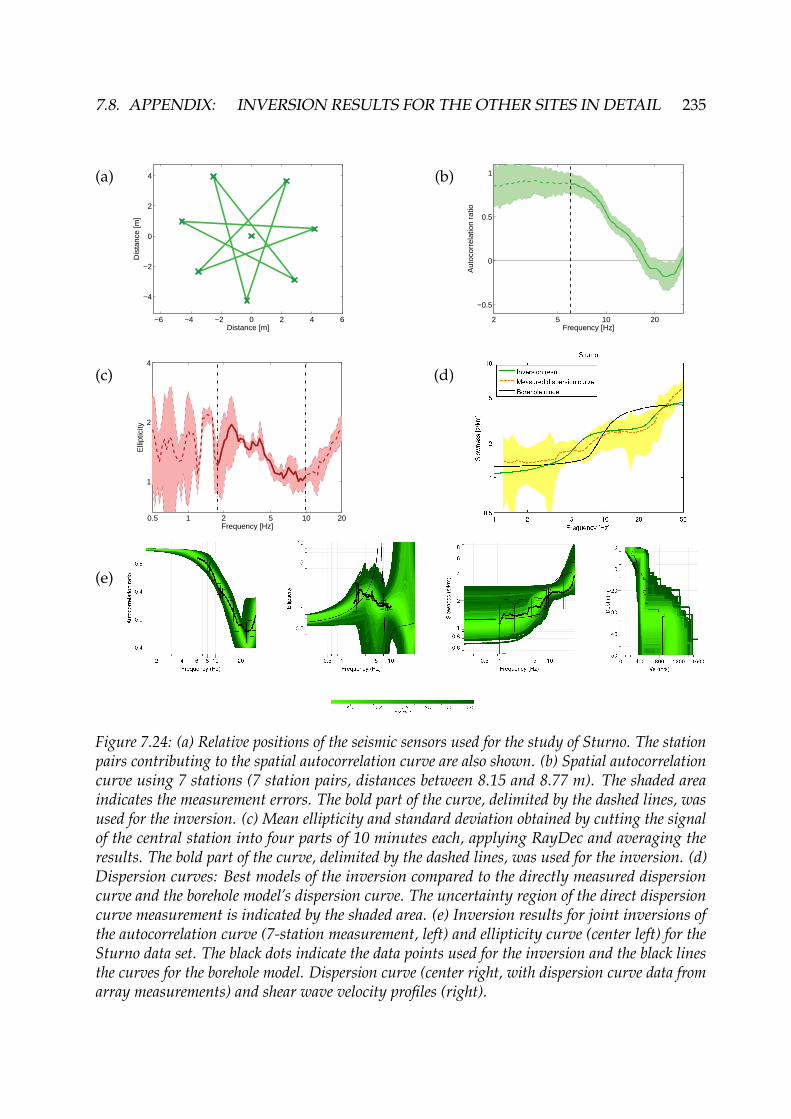
7.8. APPENDIX: INVERSION RESULTS FOR THE OTHER SITES IN DETAIL 235

(a)

−6 −4 −2 0 2 4 6

−4

−2

0

2

4

Distance [m]

Dis

tanc

e [m

]

(b)

2 5 10 20

−0.5

0

0.5

1

Frequency [Hz]

Aut

ocor

rela

tion

ratio

(c)

0.5 1 2 5 10 20

1

2

4

Frequency [Hz]

Elli

ptic

ity

(d)

(e)

Figure 7.24: (a) Relative positions of the seismic sensors used for the study of Sturno. The stationpairs contributing to the spatial autocorrelation curve are also shown. (b) Spatial autocorrelationcurve using 7 stations (7 station pairs, distances between 8.15 and 8.77 m). The shaded areaindicates the measurement errors. The bold part of the curve, delimited by the dashed lines, wasused for the inversion. (c) Mean ellipticity and standard deviation obtained by cutting the signalof the central station into four parts of 10 minutes each, applying RayDec and averaging theresults. The bold part of the curve, delimited by the dashed lines, was used for the inversion. (d)Dispersion curves: Best models of the inversion compared to the directly measured dispersioncurve and the borehole model’s dispersion curve. The uncertainty region of the direct dispersioncurve measurement is indicated by the shaded area. (e) Inversion results for joint inversions ofthe autocorrelation curve (7-station measurement, left) and ellipticity curve (center left) for theSturno data set. The black dots indicate the data points used for the inversion and the black linesthe curves for the borehole model. Dispersion curve (center right, with dispersion curve data fromarray measurements) and shear wave velocity profiles (right).

Chapter 8

Investigation of the seismological wavefield: Earthquake array measurements inCalifornia

This chapter investigates the seismological wave field generated by earthquakes. A dataset of 22 earthquakes recorded by the San Jose Dense Seismic Array in California isanalyzed using MUSIQUE. The array is located on the Evergreen Basin, near the easternedge of the Santa Clara Valley. The azimuthal energy distribution of the different eventsis compared, including for some events a comparison between the early arrivals andthe later signal. Furthermore, the energy repartition between Love and Rayleigh wavesis analyzed in different frequency ranges. Finally, the analysis results for the differentevents are combined to global dispersion and ellipticity curves of the basin.

Ce chapitre examinera le champ d’ondes sismique produit par des séismes. Un jeu de données de22 séismes enregistrés par un réseau de capteurs sismiques localisé à San Jose en Californie estanalysé avec MUSIQUE. Le réseau a été deployé sur le bassin d’Evergreen, proche de la frontièreest de la vallée de Santa Clara. La distribution d’énergie suivant l’azimut sera comparé pourles différents évènements, y inclus une comparaison entre les premières arrivées et les arrivéestardives pour quelques séismes. En outre, la répartition d’énergie entre les ondes de Love etles ondes de Rayleigh sera analysée pour différentes gammes de fréquence. Finalement, lesanalyses des différents évènements seront combinées pour déterminer des courbes de dispersionet d’ellipticité globales pour le bassin.

237

238 CHAPTER 8. INVESTIGATION OF THE SEISMOLOGICAL WAVE FIELD

8.1 Introduction

The topic of this chapter is the investigation of the seismological wave field generated byearthquakes. This analysis is performed using the MUSIQUE technique introduced in4.6. In the following, this technique will be applied to real data measurements obtainedby The San Jose Dense Seismic Array in California, a temporary array recording between1999 and 2004. The array is located near the eastern edge of the Santa Clara Valley, wheredeep sedimentary layers form the Evergreen Basin. The south-western edge of the SantaClara Valley is formed by the Cupertino basin, which is separated from the EvergreenBasin by a subsurface ridge. The geology of the Evergreen Basin is shown in figure 8.1.

Figure 8.1: (Left) Map showing the surficial geology [by Wentworth, 1997] of the Santa ClaraValley and the location of the San Jose Dense Seismic Array in the Evergreen Basin inside thevalley. In the zoom on the array (right), the array stations and the depth contour layers [byBrocher et al., 1997] of the Basin are shown in 500-m-intervals. The basin reaches a maximumdepth of about 8 km. Figure extracted from Frankel et al. [2001].

A previous study using data of the San Jose Dense Seismic Array was published byFrankel et al. [2001]. They found that the amplification of seismic waves is strongertowards the south-western edge of the Evergreen Basin. Furthermore, they observedpatterns of waves traveling across the array. For earthquakes located at the east, surfacewaves from the south follow the direct S-wave arrivals. Frankel et al. [2001] identifiedthese surface waves as Love waves which are probably generated by S-wave scatteringat the southern border of the Santa Clara Valley.Another study using the San Jose array was performed by Hartzell et al. [2003] whoinvestigated the site response for local and regional earthquakes and identified possiblewave scatterers in the valley. Hartzell et al. [2006] developed a detailed 3D velocitymodel of the Santa Clara Valley and showed the importance of surface waves for theground motion of sedimentary basins.

8.2. ARRAY SETUP AND BASIN MODEL 239

In a further study by Hartzell et al. [2010], it was shown that the maximum of amplifica-tion for the horizontal motion occurs at the southern edge of the basin, whereas it occursat the deepest parts for the vertical component. The authors suggest that this can eitherbe attributed to a different interaction of Love and Rayleigh waves with the basin shapeor that Love waves are more influenced by the lower shear wave velocity region at thesouth-western edge of the basin.Other studies investigated the same area without using the San Jose Dense Seismic Array.Fletcher et al. [2003] analyzed the data of a different array covering the whole Santa ClaraValley. They investigated the P- and S-wave arrival times from both local deep eventsand teleseismic events and found that the arrivals are delayed for stations located overthe Evergreen or Cupertino Basins, but arrive earlier for stations located on the ridgebetween both basins. Furthermore, they determined that the attenuation is larger at thebasins than on the ridge. Dolenc et al. [2005] used the same array recordings and showedthat the P-wave arrival time delays and amplification parameters for teleseismic eventsare correlated. Another study was done by Dolenc and Dreger [2005], which was basedon the same array but for microtremor records. This study indicates that the energy ofthe seismic noise recorded on the array is related to the wave height on the ocean andthat the H/V ratio for the different sensors is stable with time.The objective of our study is to perform a systematic analysis of the propagation ofsurface waves in the basin, not only for a single earthquake, but for a set of earthquakesin order to study the correlation between surface wave types (Love, Rayleigh) andearthquake characteristics (location, magnitude). Therefore, 22 regional earthquakes indistances between 4 and 600 km are selected and the repartition and azimuth angles ofLove and Rayleigh waves are investigated in different frequency ranges. Furthermore,we combine the data for the different events to obtain Love and Rayleigh wave dispersioncurves as well as Rayleigh wave ellipticity curves.

8.2 Array setup and basin model

In early 1999, the United States Geological Survey (USGS) deployed an array of Kinemet-rics K2 accelerometers, which recorded until May 2004. The different instruments wereoperated in triggered mode, i.e. did not record continuously, but only if the accelerationexceeds a predefined threshold. The array layout is shown in figure 8.2 (a) and the arrayresponse corresponding to the selected stations is shown in figure 8.2 (b). The P- andS-wave velocities along the profile marked in figure 8.2 (a) are indicated in figures 8.3 (a)and (b), respectively. Along this profile, the maximum depth of the sedimentary filling ofthe basin reaches up to 5 km. The velocity profiles were obtained using the USGS seismicvelocity model of the San Francisco Bay AreaI, which is based on the works of Brocher[2005] and Phelps et al. [2008]. Based on this model, the theoretical Rayleigh and Lovewave dispersion curves for the structure beneath the different array stations have beencalculated.

IVersion USGSBayAreaVM-08.3.0 of the model was used.This model is available at http://earthquake.usgs.gov/regional/nca/3Dgeologic/.

240 CHAPTER 8. INVESTIGATION OF THE SEISMOLOGICAL WAVE FIELD

(a)

−4 −2 0 2 4−4

−2

0

2

4

Distance [km]

Dis

tanc

e [k

m]

(b)

Figure 8.2: (a) Layout of the San Jose array. Only the marked stations have been used for thisstudy. The green line indicates the profile for which the shear and pressure wave velocities areindicated in figure 8.3. The dispersion and ellipticity curves for the station which is marked by thelarge green circle are shown in figure 8.3. (b) Theoretical array response for the array of selectedstations.

The south-western stations of the array are located on the border of the EvergreenBasin. Therefore, their dispersion curves are different from those of the central stations.Consequently, we used only the 25 seismic stations on the basin center for this study,which are indicated by the red circles in figure 8.2 (a). As the structure of the basinis rather homogeneous under these stations, their respective dispersion and ellipticitycurves are very similar as shown in figures 8.3 (c) and (d). The outliers are located onthe edges of the used array configuration. To give an example, the dispersion curvesfor the station marked by a green circle in figure 8.2 (a) are shown in figure 8.3 (e) andthe ellipticity curve is shown in figure 8.3 (f). As the velocity contrast of the model isnot very pronounced, the group slownesses of both surface wave types do not show adistinct Airy phase. Furthermore, the theoretical ellipticity curve for the fundamentalmode does not exhibit a singularity. Consequently, the motion of this mode should beretrograde at all frequencies. As the motion of the first harmonic mode is prograde, bothmodes should be distinguishable by their particle motion.

8.2. ARRAY SETUP AND BASIN MODEL 241

(a)0 2 4 6 8

6

4

2

Distance [km]

Dep

th [k

m]

NESW

VP [k

m/s

]0

1

2

3

4

5(b)

0 2 4 6 8

6

4

2

Distance [km]

Dep

th [k

m]

SW NE

VS [k

m/s

]

0

0.5

1

1.5

2

2.5

3

(c)

0.05 0.1 0.2 0.5

0.5

1

2

Frequency [Hz]

Slo

wne

ss [s

/km

]

Rayleigh wavesLove waves (d)

0.05 0.1 0.2 0.5

1

10

Frequency [Hz]

Elli

ptic

ity

(e)

0.05 0.1 0.2 0.5

0.5

1

2

Frequency [Hz]

Slo

wne

ss [s

/km

]

Rayleigh waves, fund. modeRayleigh waves, harm. modesLove waves, fund. modeLove waves, harm. modesRayleigh waves, group slownessLove waves, group slowness

(f)

0.05 0.1 0.2 0.5

1

10

Frequency [Hz]

Elli

ptic

ity

fundamental modefirst harmonic mode

Figure 8.3: (a) Pressure wave and (b) shear wave velocity profiles according to the basin modelalong the cross section indicated by the dashed line in figure 8.2 (a). (c) Dispersion curves for thefundamental Rayleigh and Love wave modes calculated for the basin model at all used stations. (d)Fundamental Rayleigh wave mode ellipticity curve calculated at all used stations. (e) Dispersioncurve for phase and group slownesses of Rayleigh and Love waves calculated for the basin modelat the central station marked in figure 8.2 (a). (f) Rayleigh wave ellipticity curve calculated forthe basin model at the same station.

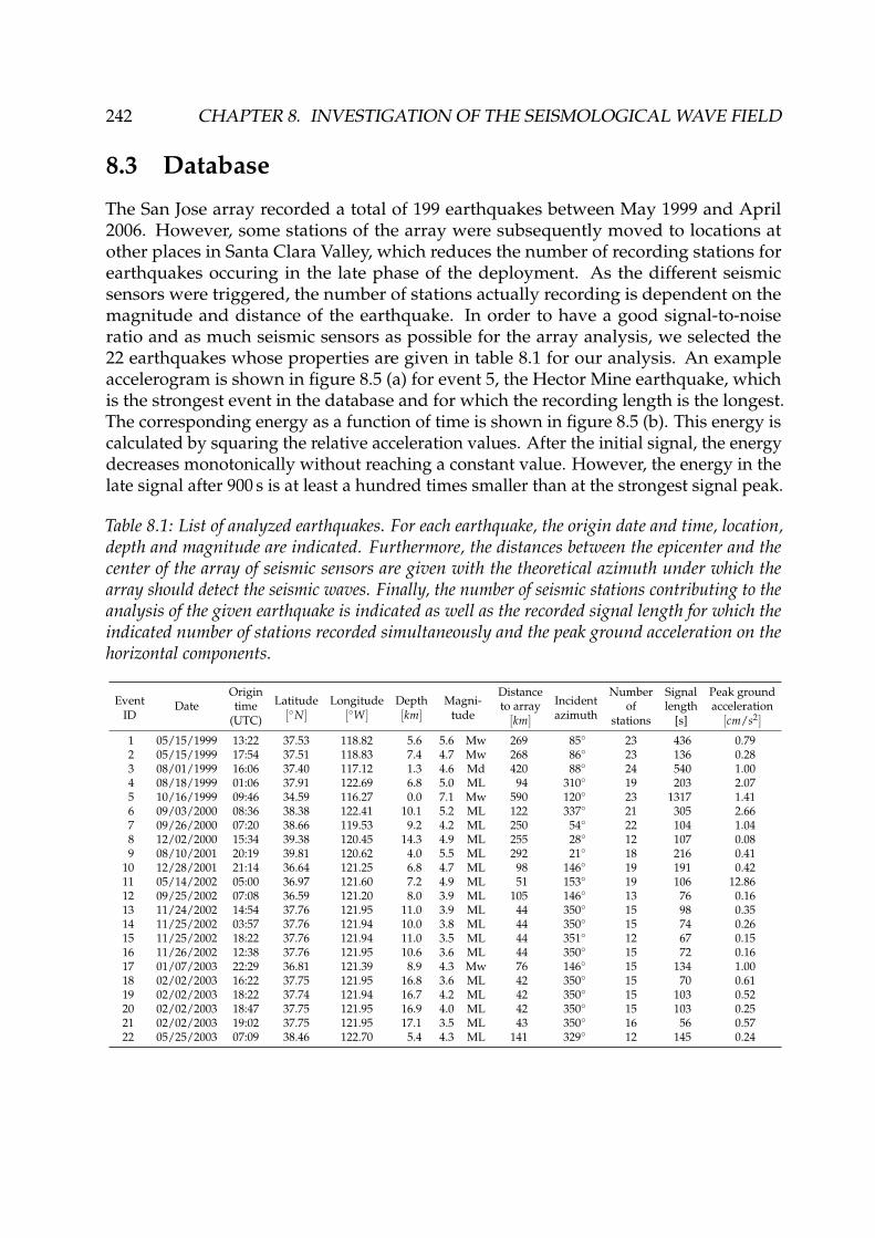
242 CHAPTER 8. INVESTIGATION OF THE SEISMOLOGICAL WAVE FIELD

8.3 Database

The San Jose array recorded a total of 199 earthquakes between May 1999 and April2006. However, some stations of the array were subsequently moved to locations atother places in Santa Clara Valley, which reduces the number of recording stations forearthquakes occuring in the late phase of the deployment. As the different seismicsensors were triggered, the number of stations actually recording is dependent on themagnitude and distance of the earthquake. In order to have a good signal-to-noiseratio and as much seismic sensors as possible for the array analysis, we selected the22 earthquakes whose properties are given in table 8.1 for our analysis. An exampleaccelerogram is shown in figure 8.5 (a) for event 5, the Hector Mine earthquake, whichis the strongest event in the database and for which the recording length is the longest.The corresponding energy as a function of time is shown in figure 8.5 (b). This energy iscalculated by squaring the relative acceleration values. After the initial signal, the energydecreases monotonically without reaching a constant value. However, the energy in thelate signal after 900 s is at least a hundred times smaller than at the strongest signal peak.

Table 8.1: List of analyzed earthquakes. For each earthquake, the origin date and time, location,depth and magnitude are indicated. Furthermore, the distances between the epicenter and thecenter of the array of seismic sensors are given with the theoretical azimuth under which thearray should detect the seismic waves. Finally, the number of seismic stations contributing to theanalysis of the given earthquake is indicated as well as the recorded signal length for which theindicated number of stations recorded simultaneously and the peak ground acceleration on thehorizontal components.

Origin Distance Number Signal Peak groundEvent Date time Latitude Longitude Depth Magni- to array Incident of length acceleration

ID (UTC) [◦N] [◦W] [km] tude [km] azimuth stations [s] [cm/s2]

1 05/15/1999 13:22 37.53 118.82 5.6 5.6 Mw 269 85◦ 23 436 0.792 05/15/1999 17:54 37.51 118.83 7.4 4.7 Mw 268 86◦ 23 136 0.283 08/01/1999 16:06 37.40 117.12 1.3 4.6 Md 420 88◦ 24 540 1.004 08/18/1999 01:06 37.91 122.69 6.8 5.0 ML 94 310◦ 19 203 2.075 10/16/1999 09:46 34.59 116.27 0.0 7.1 Mw 590 120◦ 23 1317 1.416 09/03/2000 08:36 38.38 122.41 10.1 5.2 ML 122 337◦ 21 305 2.667 09/26/2000 07:20 38.66 119.53 9.2 4.2 ML 250 54◦ 22 104 1.048 12/02/2000 15:34 39.38 120.45 14.3 4.9 ML 255 28◦ 12 107 0.089 08/10/2001 20:19 39.81 120.62 4.0 5.5 ML 292 21◦ 18 216 0.41

10 12/28/2001 21:14 36.64 121.25 6.8 4.7 ML 98 146◦ 19 191 0.4211 05/14/2002 05:00 36.97 121.60 7.2 4.9 ML 51 153◦ 19 106 12.8612 09/25/2002 07:08 36.59 121.20 8.0 3.9 ML 105 146◦ 13 76 0.1613 11/24/2002 14:54 37.76 121.95 11.0 3.9 ML 44 350◦ 15 98 0.3514 11/25/2002 03:57 37.76 121.94 10.0 3.8 ML 44 350◦ 15 74 0.2615 11/25/2002 18:22 37.76 121.94 11.0 3.5 ML 44 351◦ 12 67 0.1516 11/26/2002 12:38 37.76 121.95 10.6 3.6 ML 44 350◦ 15 72 0.1617 01/07/2003 22:29 36.81 121.39 8.9 4.3 Mw 76 146◦ 15 134 1.0018 02/02/2003 16:22 37.75 121.95 16.8 3.6 ML 42 350◦ 15 70 0.6119 02/02/2003 18:22 37.74 121.94 16.7 4.2 ML 42 350◦ 15 103 0.5220 02/02/2003 18:47 37.75 121.95 16.9 4.0 ML 42 350◦ 15 103 0.2521 02/02/2003 19:02 37.75 121.95 17.1 3.5 ML 43 350◦ 16 56 0.5722 05/25/2003 07:09 38.46 122.70 5.4 4.3 ML 141 329◦ 12 145 0.24

8.3. DATABASE 243

Figure 8.4: Map showing the epicenters of the analyzed earthquakes with respect to the location ofthe San Jose array. The diameter of the circles indicates the magnitude of the respective earthquake.

244 CHAPTER 8. INVESTIGATION OF THE SEISMOLOGICAL WAVE FIELD

(a) (b)

0 250 500 750 1000 125010

3

104

105

106

107

108

109

Time [s]

Ene

rgy

VerticalEastNorth

Figure 8.5: (a) Relative accelerogram for the three components of the station marked in figure 8.2(a) recorded during event 5. (b) The corresponding energy of the signal as a function of time. Thevertical lines delimitate the early signal including the first arrivals and the late signal which areboth used in the following.

8.4 Data processing

The signal recordings for each of the events shown in table 8.1 have been analyzed inthe following way. The signals of those of the 25 stations marked by a red circle infigure 8.2 (a) which recorded the event (i.e. for which the signal was strong enough totrigger the recording) form the array recording. The number of array stations whichrecorded the respective event is also given in table 8.1. The signals have been analyzedusing MUSIQUE (see section 4.6) for 50 different frequency values between 0.05 and0.5 Hz, using a logarithmic frequency scale. This frequency range was chosen using thebasin model’s dispersion curves (figure 8.3 (e)) in combination with the array response(figure 8.2 (b)). According to both information, the dispersion curve can be best retrievedbetween 0.1 and 0.5 Hz. Below 0.1 Hz, however, the recordings for most events are ofvery low energy.The actual signal processing was performed as described in the following. The signalsare prefiltered using a Chebyshev filter with a bandwidth of 0.1 times the respectivefrequency. For example, analyzing the signal at 0.2 Hz, the signal is filtered between0.19 and 0.21 Hz. Then, the signals are cut in time windows of three periods length.For each time window, the wave vector, i.e. azimuth and slowness, of the dominantsignal is determined using the classical MUSIC algorithm. Then, the signal is projectedin the identified azimuth direction to separate the transverse and radial components.The energy contents of the three components are calculated using the squared absolutevalues of the Fourier transform for 5 frequency values around the analyzed frequency.Based on the energy of the respective components, the algorithm identifies Love waves(if the transverse energy exceeds the sum of the radial and vertical energies) and possibleRayleigh waves (in the opposite case). If the wave is identified as a possible Rayleighwave, its polarization parameters are estimated by using quaternion-MUSIC.

8.5. AZIMUTHAL ENERGY DISTRIBUTION 245

The final Rayleigh wave identification is based on the estimation of the phase differenceϕ: For 45◦ < ϕ < 135◦, the wave is identified as retrograde Rayleigh wave, for 225◦ <ϕ < 315◦ as prograde wave and for other values, it is left unclassified.

8.5 Azimuthal energy distribution

8.5.1 Comparison between the the early and late signals

According to table 8.1, there are four earthquakes (events 1, 3, 5 and 6) for which therecorded signal duration is significantly longer than three minutes. The beginning ofthe record for these events is clearly dominated by the arrival of direct waves fromthe earthquake. Once these waves have left the array, the signal will exhibit featureslinked to the basin structure. Therefore, analyzing the beginning and end of these signalsindependently can teach us on the basin structure from its effects on the seismologicalwave field. Phillips and Aki [1986] and Riepl et al. [1998] suggested that the beginning ofthe coda of earthquake data starts at about two times the shear wave travel time from theearthquake to the array. To be in the safe range, in our investigation of the early arrivals,the early signal ends at about 1.5 times the shear wave travel time. Due to the use ofaccelerometers, for most events, the signals are of very low energy at low frequencies(around 0.1 Hz).

8.5.1.1 Event 1

In figure 8.6, the energy distribution with respect to the incident angle for event 1 isplotted for Rayleigh and Love waves in different frequency ranges. The energy distribu-tion for the first 75 seconds of signal is indicated in figure 8.6 (a), for the signal after 200seconds in figure 8.6 (b). The relative energy distributions of Rayleigh and Love waveswhich are indicated by the respective diagrams are normalized in such way that the sumof the total energies of Love and Rayleigh waves over all frequency ranges equals 1. Inthe figure below, it is indicated which part of the total energy in the respective frequencyrange is carried by the identified Love and Rayleigh waves.In all frequency ranges, the main first Love wave arrivals are principally oriented in thetheoretical azimuth direction, i.e. arriving under an azimuth of 85◦. The small deviationsto the north can be explained by wave refraction on the eastern basin edge. Actually, thenorth-western to south-eastern orientation of the basin refracts waves arriving from theeast by some degrees to the south, so that the array detects them from a direction shiftedto the north.

At frequencies below 0.2 Hz, Rayleigh waves arrive principally from the theoreticalazimuth, but their amplitude is very low. At higher frequencies, they are still arrivingfrom eastern directions, but are more scattered than Love waves.In the late arrivals, the Love wave energy is slightly larger than the Rayleigh wave energy.Nevertheless, the energy content in the first signal (the first 75 s) is ten times higher thanin this late signal (after 200 s). At all frequencies, a dominant Love wave contributionarriving from the south can be seen, with minor contributions from other directions.

246 CHAPTER 8. INVESTIGATION OF THE SEISMOLOGICAL WAVE FIELD

This signal from the south has already been observed by Frankel et al. [2001] whoattributed it to a scattered Love wave. The scatterer could either be a large rock formationlocated south of the array or the southern basin edge. For Rayleigh waves, the energydistribution is rather inhomogeneous, but at lower frequencies (below 0.3 Hz), wavesarrive principally from the north-west, whereas the principal direction is south-east forhigher frequencies.

8.5.1.2 Event 3

Event 3 is located at the same azimuth (88◦), but in a larger distance than event 1. Theazimuthal energy distribution for this event is shown in figure 8.7 both for the first 110seconds of signal (a) and for the signal after 250 seconds (b). Both Love and Rayleighwaves arrive principally from the theoretical azimuth. Between 0.2 and 0.3 Hz, however,the Love wave arrival is dominated by the southern direction. For the late signal arrivals,a large part of energy is still arriving from the main azimuth. Between 0.15 and 0.2 Hz,however, both wave types are arriving under a large variety of azimuths. In the nextfrequency band between 0.2 and 0.3 Hz, Love waves exhibit three principal azimuths:north, the theoretical azimuth and south.

8.5.1.3 Event 5

Event 5 represents the Hector Mine earthquake, with a magnitude of 7.1 the largestrecorded earthquake in the data set. With a recording length of 22 minutes, it representsthe longest record, too. The earthquake was located at a theoretical azimuth of 120◦.In figure 8.8, the azimuthal energy distributions of the first 180 seconds of signal aswell as for the signal after 900 seconds are shown for different frequency ranges. In thebeginning of the signal, waves are mainly arriving from south-eastern directions, butslightly shifted from the theoretical azimuth. At low frequencies (below 0.15 Hz), Lovewaves arrive under azimuths slightly shifted to the north, whereas for higher frequencies,a large amount of Love wave energy is arriving from the south. This azimuth was alreadydominant for the late arrivals of event 1. For Rayleigh waves, no systematic behaviorcan be observed.In the late arrivals, smaller amounts of Love waves can be observed from differentazimuths, but the main energy contribution is associated to the frequency range between0.15 and 0.2 Hz, where the waves are mainly arriving from the east, and to the frequencyrange between 0.2 and 0.3 Hz, where the waves are principally arriving from the south.Here again, Rayleigh waves are more scattered with a multitude of azimuths, but themain energy arrives from southern to south-eastern directions.

8.5. AZIMUTHAL ENERGY DISTRIBUTION 247

8.5.1.4 Event 6

The last event of longer duration is event 6, located under an azimuth of 337◦, i.e. inthe north of the Santa Clara Valley. The azimuthal energy distributions associated tothe first 50 seconds of this signal as well as for the signal after 150 seconds are shownin figure 8.9. In the early signal, the energy is concentrated around the theoretical az-imuth. Nevertheless, most of the Love waves are arriving under azimuths which aresystematically shifted, e.g. around 0◦ for the frequency range between 0.2 and 0.4 Hz.These waves could be direct waves which have been reflected once or multiple timesat the basin borders. Rayleigh waves are of very low energy below 0.4 Hz. Above thatfrequency, most of the energy is arriving from the direct azimuth.For the late signal, the azimuthal energy distribution is wider with more azimuths in-volved, but no energy arrives from south-eastern directions. However, the most energeticLove wave arrival in this signal part is associated to azimuths centered around thetheoretical azimuth. For Rayleigh waves, the energy distribution is wider and morewaves arrive from azimuths different from the main azimuth.

248 CHAPTER 8. INVESTIGATION OF THE SEISMOLOGICAL WAVE FIELD

(a) Event 1 - first 75 s of signal

0

30

60

90

120

150

180

210

240

270

300

330

0.05 − 0.10 Hz

RayleighLove

0

30

60

90

120

150

180

210

240

270

300

330

0.10 − 0.15 Hz

RayleighLove

0

30

60

90

120

150

180

210

240

270

300

330

0.15 − 0.20 Hz

RayleighLove

0.05 0.1 0.15 0.2 0.3 0.4 0.50

0.1

0.2

0.3

Frequency range [Hz]

Ene

rgy

RayleighLove

0

30

60

90

120

150

180

210

240

270

300

330

0.20 − 0.30 Hz

RayleighLove

0

30

60

90

120

150

180

210

240

270

300

330

0.30 − 0.40 Hz

RayleighLove

0

30

60

90

120

150

180

210

240

270

300

330

0.40 − 0.50 Hz

RayleighLove

0.05 0.1 0.15 0.2 0.3 0.4 0.50

20

40

60

80

100

Frequency range [Hz]

Iden

tifie

d en

ergy

[% o

f tot

al e

nerg

y]

(b) Event 1 - signal after 200 s

0

30

60

90

120

150

180

210

240

270

300

330

0.05 − 0.10 Hz

RayleighLove

0

30

60

90

120

150

180

210

240

270

300

330

0.10 − 0.15 Hz

RayleighLove

0

30

60

90

120

150

180

210

240

270

300

330

0.15 − 0.20 Hz

RayleighLove

0.05 0.1 0.15 0.2 0.3 0.4 0.50

0.1

0.2

Frequency range [Hz]

Ene

rgy

RayleighLove

0

30

60

90

120

150

180

210

240

270

300

330

0.20 − 0.30 Hz

RayleighLove

0

30

60

90

120

150

180

210

240

270

300

330

0.30 − 0.40 Hz

RayleighLove

0

30

60

90

120

150

180

210

240

270

300

330

0.40 − 0.50 Hz

RayleighLove

0.05 0.1 0.15 0.2 0.3 0.4 0.50

20

40

60

80

100

Frequency range [Hz]

Iden

tifie

d en

ergy

[% o

f tot

al e

nerg

y]

Figure 8.6: Azimuthal energy distribution for different frequency ranges for (a) the first 75 s ofsignal of event 1 and (b) the signal after 200 s, i.e. after all direct waves have passed the array(bottom). The blue dot indicates the theoretical azimuth of the event. For clarity reasons, thecurves for Rayleigh and Love waves are normalized by their respective maxima. The figure ontop at the right side indicates the relative energy distribution of both wave types in the respectivefrequency bands. The figure below indicates the percentage of the total energy in the respectivefrequency range which is carried by identified Love and Rayleigh waves.

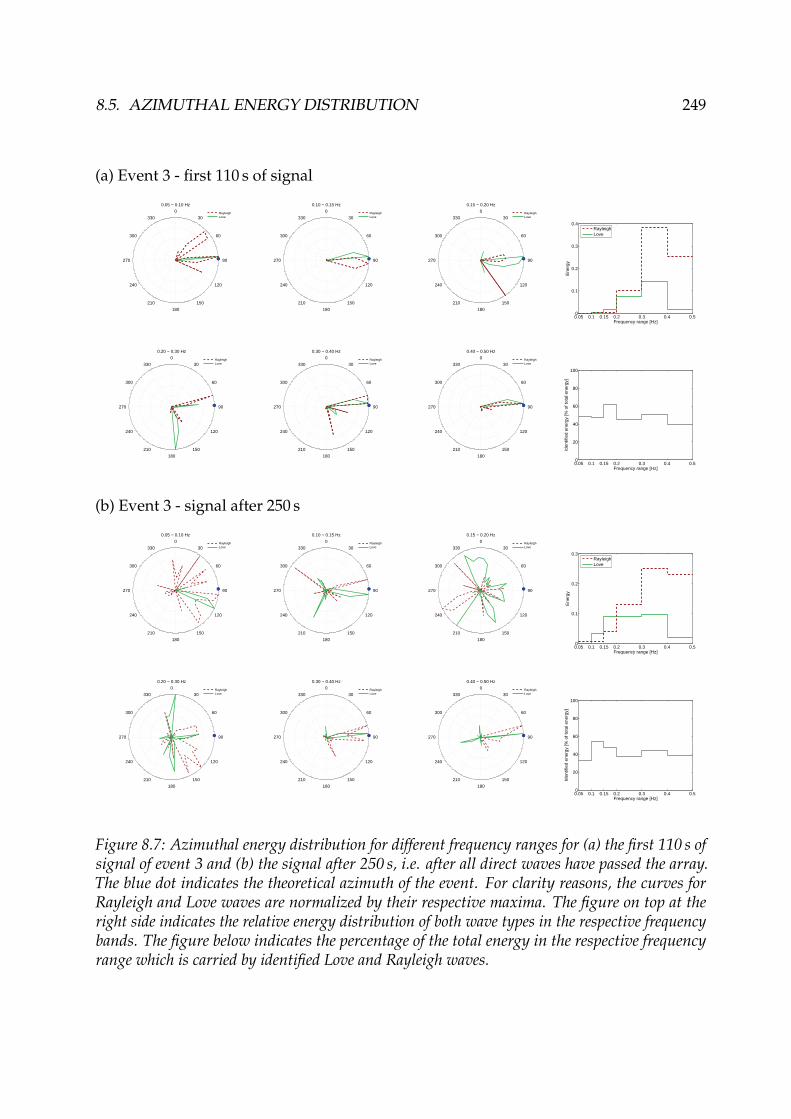
8.5. AZIMUTHAL ENERGY DISTRIBUTION 249

(a) Event 3 - first 110 s of signal

0

30

60

90

120

150

180

210

240

270

300

330

0.05 − 0.10 Hz

RayleighLove

0

30

60

90

120

150

180

210

240

270

300

330

0.10 − 0.15 Hz

RayleighLove

0

30

60

90

120

150

180

210

240

270

300

330

0.15 − 0.20 Hz

RayleighLove

0.05 0.1 0.15 0.2 0.3 0.4 0.50

0.1

0.2

0.3

0.4

Frequency range [Hz]

Ene

rgy

RayleighLove

0

30

60

90

120

150

180

210

240

270

300

330

0.20 − 0.30 Hz

RayleighLove

0

30

60

90

120

150

180

210

240

270

300

330

0.30 − 0.40 Hz

RayleighLove

0

30

60

90

120

150

180

210

240

270

300

330

0.40 − 0.50 Hz

RayleighLove

0.05 0.1 0.15 0.2 0.3 0.4 0.50

20

40

60

80

100

Frequency range [Hz]

Iden

tifie

d en

ergy

[% o

f tot

al e

nerg

y]

(b) Event 3 - signal after 250 s

0

30

60

90

120

150

180

210

240

270

300

330

0.05 − 0.10 Hz

RayleighLove

0

30

60

90

120

150

180

210

240

270

300

330

0.10 − 0.15 Hz

RayleighLove

0

30

60

90

120

150

180

210

240

270

300

330

0.15 − 0.20 Hz

RayleighLove

0.05 0.1 0.15 0.2 0.3 0.4 0.50

0.1

0.2

0.3

Frequency range [Hz]

Ene

rgy

RayleighLove

0

30

60

90

120

150

180

210

240

270

300

330

0.20 − 0.30 Hz

RayleighLove

0

30

60

90

120

150

180

210

240

270

300

330

0.30 − 0.40 Hz

RayleighLove

0

30

60

90

120

150

180

210

240

270

300

330

0.40 − 0.50 Hz

RayleighLove

0.05 0.1 0.15 0.2 0.3 0.4 0.50

20

40

60

80

100

Frequency range [Hz]

Iden

tifie

d en

ergy

[% o

f tot

al e

nerg

y]

Figure 8.7: Azimuthal energy distribution for different frequency ranges for (a) the first 110 s ofsignal of event 3 and (b) the signal after 250 s, i.e. after all direct waves have passed the array.The blue dot indicates the theoretical azimuth of the event. For clarity reasons, the curves forRayleigh and Love waves are normalized by their respective maxima. The figure on top at theright side indicates the relative energy distribution of both wave types in the respective frequencybands. The figure below indicates the percentage of the total energy in the respective frequencyrange which is carried by identified Love and Rayleigh waves.

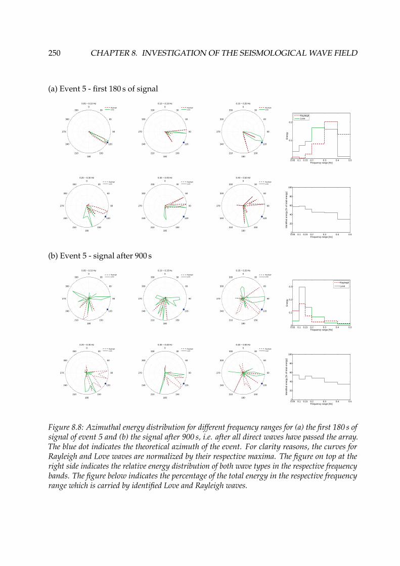
250 CHAPTER 8. INVESTIGATION OF THE SEISMOLOGICAL WAVE FIELD

(a) Event 5 - first 180 s of signal

0

30

60

90

120

150

180

210

240

270

300

330

0.05 − 0.10 Hz

RayleighLove

0

30

60

90

120

150

180

210

240

270

300

330

0.10 − 0.15 Hz

RayleighLove

0

30

60

90

120

150

180

210

240

270

300

330

0.15 − 0.20 Hz

RayleighLove

0.05 0.1 0.15 0.2 0.3 0.4 0.50

0.1

0.2

Frequency range [Hz]

Ene

rgy

RayleighLove

0

30

60

90

120

150

180

210

240

270

300

330

0.20 − 0.30 Hz

RayleighLove

0

30

60

90

120

150

180

210

240

270

300

330

0.30 − 0.40 Hz

RayleighLove

0

30

60

90

120

150

180

210

240

270

300

330

0.40 − 0.50 Hz

RayleighLove

0.05 0.1 0.15 0.2 0.3 0.4 0.50

20

40

60

80

100

Frequency range [Hz]

Iden

tifie

d en

ergy

[% o

f tot

al e

nerg

y]

(b) Event 5 - signal after 900 s

0

30

60

90

120

150

180

210

240

270

300

330

0.05 − 0.10 Hz

RayleighLove

0

30

60

90

120

150

180

210

240

270

300

330

0.10 − 0.15 Hz

RayleighLove

0

30

60

90

120

150

180

210

240

270

300

330

0.15 − 0.20 Hz

RayleighLove

0.05 0.1 0.15 0.2 0.3 0.4 0.50

0.1

0.2

0.3

Frequency range [Hz]

Ene

rgy

Rayleigh

Love

0

30

60

90

120

150

180

210

240

270

300

330

0.20 − 0.30 Hz

RayleighLove

0

30

60

90

120

150

180

210

240

270

300

330

0.30 − 0.40 Hz

RayleighLove

0

30

60

90

120

150

180

210

240

270

300

330

0.40 − 0.50 Hz

RayleighLove

0.05 0.1 0.15 0.2 0.3 0.4 0.50

20

40

60

80

100

Frequency range [Hz]

Iden

tifie

d en

ergy

[% o

f tot

al e

nerg

y]

Figure 8.8: Azimuthal energy distribution for different frequency ranges for (a) the first 180 s ofsignal of event 5 and (b) the signal after 900 s, i.e. after all direct waves have passed the array.The blue dot indicates the theoretical azimuth of the event. For clarity reasons, the curves forRayleigh and Love waves are normalized by their respective maxima. The figure on top at theright side indicates the relative energy distribution of both wave types in the respective frequencybands. The figure below indicates the percentage of the total energy in the respective frequencyrange which is carried by identified Love and Rayleigh waves.

8.5. AZIMUTHAL ENERGY DISTRIBUTION 251

(a) Event 6 - first 50 s of signal

0

30

60

90

120

150

180

210

240

270

300

330

0.05 − 0.10 Hz

Rayleigh 0

30

60

90

120

150

180

210

240

270

300

330

0.10 − 0.15 Hz

Rayleigh 0

30

60

90

120

150

180

210

240

270

300

330

0.15 − 0.20 Hz

RayleighLove

0.05 0.1 0.15 0.2 0.3 0.4 0.50

0.1

0.2

0.3

0.4

0.5

Frequency range [Hz]

Ene

rgy

RayleighLove

0

30

60

90

120

150

180

210

240

270

300

330

0.20 − 0.30 Hz

RayleighLove

0

30

60

90

120

150

180

210

240

270

300

330

0.30 − 0.40 Hz

RayleighLove

0

30

60

90

120

150

180

210

240

270

300

330

0.40 − 0.50 Hz

RayleighLove

0.05 0.1 0.15 0.2 0.3 0.4 0.50

20

40

60

80

100

Frequency range [Hz]

Iden

tifie

d en

ergy

[% o

f tot

al e

nerg

y]

(b) Event 6 - signal after 150 s

0

30

60

90

120

150

180

210

240

270

300

330

0.05 − 0.10 Hz

Rayleigh 0

30

60

90

120

150

180

210

240

270

300

330

0.10 − 0.15 Hz

RayleighLove

0

30

60

90

120

150

180

210

240

270

300

330

0.15 − 0.20 Hz

RayleighLove

0.05 0.1 0.15 0.2 0.3 0.4 0.50

0.1

0.2

0.3

0.4

Frequency range [Hz]

Ene

rgy

RayleighLove

0

30

60

90

120

150

180

210

240

270

300

330

0.20 − 0.30 Hz

RayleighLove

0

30

60

90

120

150

180

210

240

270

300

330

0.30 − 0.40 Hz

RayleighLove

0

30

60

90

120

150

180

210

240

270

300

330

0.40 − 0.50 Hz

RayleighLove

0.05 0.1 0.15 0.2 0.3 0.4 0.50

20

40

60

80

100

Frequency range [Hz]

Iden

tifie

d en

ergy

[% o

f tot

al e

nerg

y]

Figure 8.9: Azimuthal energy distribution for different frequency ranges for (a) the first 50 s ofsignal of event 6 and (b) the signal after 150 s, i.e. after all direct waves have passed the array.The blue dot indicates the theoretical azimuth of the event. For clarity reasons, the curves forRayleigh and Love waves are normalized by their respective maxima. The figure on top at theright side indicates the relative energy distribution of both wave types in the respective frequencybands. The figure below indicates the percentage of the total energy in the respective frequencyrange which is carried by identified Love and Rayleigh waves.

252 CHAPTER 8. INVESTIGATION OF THE SEISMOLOGICAL WAVE FIELD

8.5.2 Temporal Love wave azimuth evolutionIn figures 8.6, 8.7 and 8.8, a large amount of Love waves arriving from the south wasidentified. The main frequency range of these arrivals lies between 0.15 and 0.3 Hz.Therefore, the temporal evolution of the azimuth of Love waves in this frequency rangeis shown in figure 8.10 for the events 1, 5 and 6. Figure 8.6 indicated that the early Lovewave field is dominated by arrivals from the theoretical azimuth direction, whereas thelate wave field is dominated by arrivals from the south. This effect can also be seenin figure 8.10. In all analyzed frequency bands, the first arrivals come approximatelyfrom the direct azimuth, slightly deviated to the north. Later arrivals are dominated bywaves arriving at azimuths of 180◦. For frequencies between 0.25 and 0.30 Hz, both mainazimuths are not well separated, i.e. arrivals from 180◦ are directly following arrivalsfrom 90◦ and vice versa.For event 5, due to the length of the signal, a lot more time windows have been analyzed.Between 0.15 and 0.20 Hz, waves arrive under all azimuths between 60 and 180◦ duringthe whole signal length. In the next frequency range (0.20 - 0.25 Hz), two principalazimuths at 90◦ and 160◦ can be identified, but waves arrive as well from azimuthsbetween these two values. In the frequency range between 0.25 and 0.30 Hz, finally,waves arrive almost exclusively from two distinct directions, 90◦ and 180◦. The firstarrivals in these frequency range are not coming from the direct azimuth, but fromsouthern directions. However, in all frequency ranges, the azimuthal energy distributiondoes not change much with time. Towards the end of the signal, some low-energyarrivals from azimuths different from the two main directions can be seen.For events 1 and 5, the deviation of the direct arrivals (75◦ instead of 85◦ for event 1, 90◦

instead of 120◦ for event 5) can be explained by refraction of the direct waves at the basinborders. The arrivals from the south in both events can be explained by a large scattererlocated at the south. This result has already been found by Frankel et al. [2001].For event 6, the theoretical azimuth is 337◦ and the source is located in north of the SantaClara Valley. For the frequency range between 0.15 and 0.20 Hz, the main Love waveazimuth is about 270◦. However, the very first arrivals are in the theoretical azimuth. Thesame can be observed for larger frequencies (0.20 - 0.25 Hz), but another part of the signalis arriving with azimuths around 0◦. In the frequency range from 0.25 to 0.30 Hz, finally,the main part of the energy is arriving under azimuths around 0◦, including the firstarrival. Some later energy is arriving from 270◦, too. Here again, the principal energydistribution is rather constant in time. These results can be explained by the location ofthe source in the approximate extension of the basin. Waves originating at the sourceare reflected at the lateral basin borders. The array detects these waves as arrivals fromlarger or lower azimuth values.

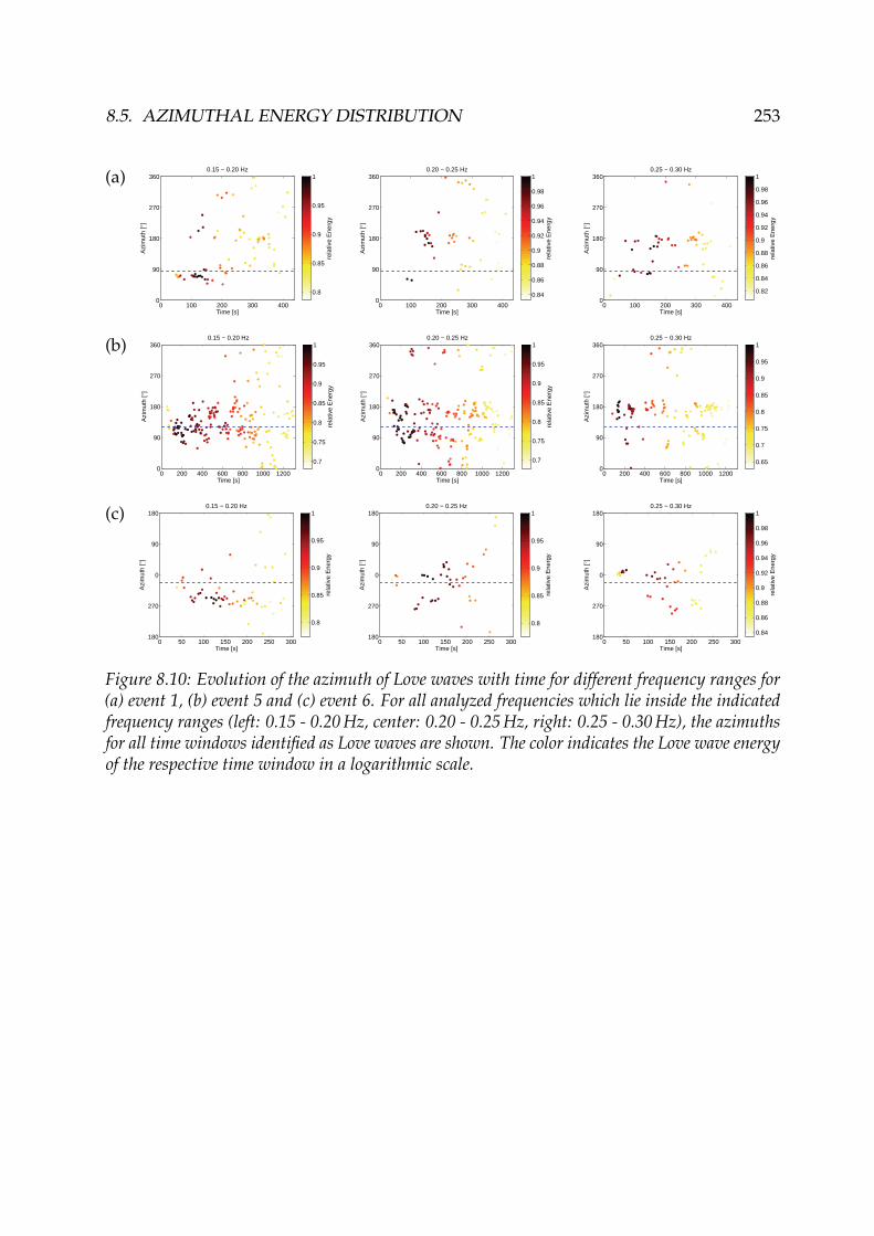
8.5. AZIMUTHAL ENERGY DISTRIBUTION 253

(a)

0 100 200 300 4000

90

180

270

360

Time [s]

Azi

mut

h [°

]

0.15 − 0.20 Hz

rela

tive

Ene

rgy

0.8

0.85

0.9

0.95

1

0 100 200 300 4000

90

180

270

360

Time [s]

Azi

mut

h [°

]

0.20 − 0.25 Hz

rela

tive

Ene

rgy

0.84

0.86

0.88

0.9

0.92

0.94

0.96

0.98

1

0 100 200 300 4000

90

180

270

360

Time [s]

Azi

mut

h [°

]

0.25 − 0.30 Hz

rela

tive

Ene

rgy

0.82

0.84

0.86

0.88

0.9

0.92

0.94

0.96

0.98

1

(b)

0 200 400 600 800 1000 12000

90

180

270

360

Time [s]

Azi

mut

h [°

]

0.15 − 0.20 Hz

rela

tive

Ene

rgy

0.7

0.75

0.8

0.85

0.9

0.95

1

0 200 400 600 800 1000 12000

90

180

270

360

Time [s]

Azi

mut

h [°

]

0.20 − 0.25 Hz

rela

tive

Ene

rgy

0.7

0.75

0.8

0.85

0.9

0.95

1

0 200 400 600 800 1000 12000

90

180

270

360

Time [s]

Azi

mut

h [°

]

0.25 − 0.30 Hz

0.65

0.7

0.75

0.8

0.85

0.9

0.95

1

(c)

0 50 100 150 200 250 300180

270

0

90

180

Time [s]

Azi

mut

h [°

]

0.15 − 0.20 Hz

rela

tive

Ene

rgy

0.8

0.85

0.9

0.95

1

0 50 100 150 200 250 300180

270

0

90

180

Time [s]

Azi

mut

h [°

]

0.20 − 0.25 Hz

rela

tive

Ene

rgy

0.8

0.85

0.9

0.95

1

0 50 100 150 200 250 300180

270

0

90

180

Time [s]

Azi

mut

h [°

]

0.25 − 0.30 Hz

rela

tive

Ene

rgy

0.84

0.86

0.88

0.9

0.92

0.94

0.96

0.98

1

Figure 8.10: Evolution of the azimuth of Love waves with time for different frequency ranges for(a) event 1, (b) event 5 and (c) event 6. For all analyzed frequencies which lie inside the indicatedfrequency ranges (left: 0.15 - 0.20 Hz, center: 0.20 - 0.25 Hz, right: 0.25 - 0.30 Hz), the azimuthsfor all time windows identified as Love waves are shown. The color indicates the Love wave energyof the respective time window in a logarithmic scale.

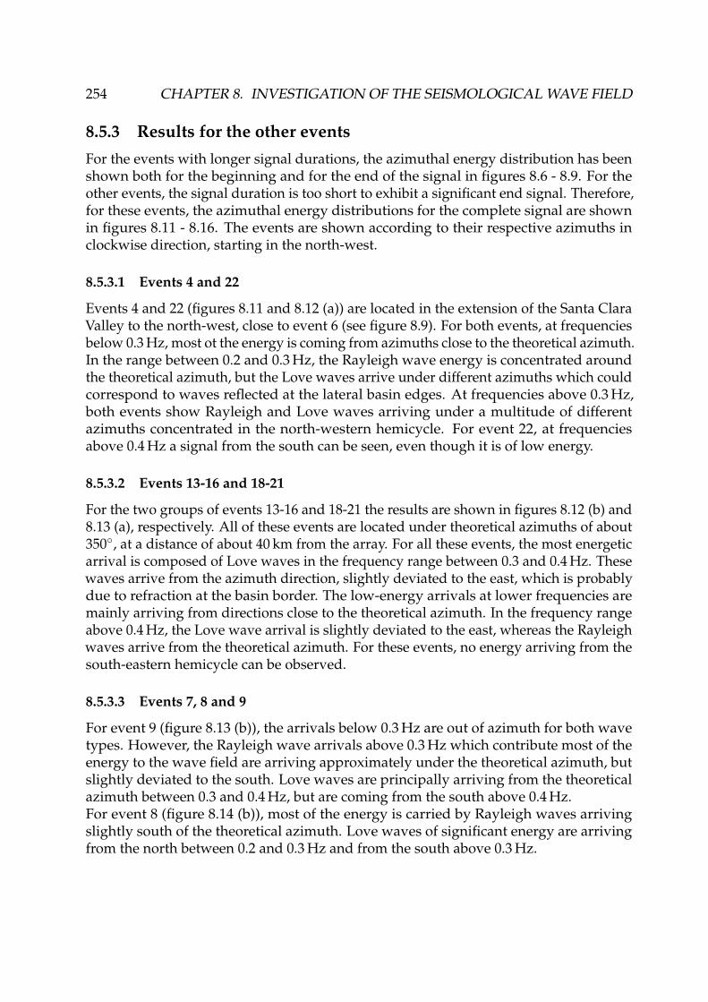
254 CHAPTER 8. INVESTIGATION OF THE SEISMOLOGICAL WAVE FIELD

8.5.3 Results for the other eventsFor the events with longer signal durations, the azimuthal energy distribution has beenshown both for the beginning and for the end of the signal in figures 8.6 - 8.9. For theother events, the signal duration is too short to exhibit a significant end signal. Therefore,for these events, the azimuthal energy distributions for the complete signal are shownin figures 8.11 - 8.16. The events are shown according to their respective azimuths inclockwise direction, starting in the north-west.

8.5.3.1 Events 4 and 22

Events 4 and 22 (figures 8.11 and 8.12 (a)) are located in the extension of the Santa ClaraValley to the north-west, close to event 6 (see figure 8.9). For both events, at frequenciesbelow 0.3 Hz, most ot the energy is coming from azimuths close to the theoretical azimuth.In the range between 0.2 and 0.3 Hz, the Rayleigh wave energy is concentrated aroundthe theoretical azimuth, but the Love waves arrive under different azimuths which couldcorrespond to waves reflected at the lateral basin edges. At frequencies above 0.3 Hz,both events show Rayleigh and Love waves arriving under a multitude of differentazimuths concentrated in the north-western hemicycle. For event 22, at frequenciesabove 0.4 Hz a signal from the south can be seen, even though it is of low energy.

8.5.3.2 Events 13-16 and 18-21

For the two groups of events 13-16 and 18-21 the results are shown in figures 8.12 (b) and8.13 (a), respectively. All of these events are located under theoretical azimuths of about350◦, at a distance of about 40 km from the array. For all these events, the most energeticarrival is composed of Love waves in the frequency range between 0.3 and 0.4 Hz. Thesewaves arrive from the azimuth direction, slightly deviated to the east, which is probablydue to refraction at the basin border. The low-energy arrivals at lower frequencies aremainly arriving from directions close to the theoretical azimuth. In the frequency rangeabove 0.4 Hz, the Love wave arrival is slightly deviated to the east, whereas the Rayleighwaves arrive from the theoretical azimuth. For these events, no energy arriving from thesouth-eastern hemicycle can be observed.

8.5.3.3 Events 7, 8 and 9

For event 9 (figure 8.13 (b)), the arrivals below 0.3 Hz are out of azimuth for both wavetypes. However, the Rayleigh wave arrivals above 0.3 Hz which contribute most of theenergy to the wave field are arriving approximately under the theoretical azimuth, butslightly deviated to the south. Love waves are principally arriving from the theoreticalazimuth between 0.3 and 0.4 Hz, but are coming from the south above 0.4 Hz.For event 8 (figure 8.14 (b)), most of the energy is carried by Rayleigh waves arrivingslightly south of the theoretical azimuth. Love waves of significant energy are arrivingfrom the north between 0.2 and 0.3 Hz and from the south above 0.3 Hz.

8.5. AZIMUTHAL ENERGY DISTRIBUTION 255

For event 7 (figure 8.14 (b)), the dominant Rayleigh wave arrivals are exactly in thetheoretical azimuth direction for all frequencies above 0.15 Hz. The Love wave arrivalsare more scattered, but the most energetic Love waves in the range from 0.2 to 0.4 Hz arecoming from the south. The arrival of Rayleigh waves from the exact theoretical azimuthmight be explained by the fact that the theoretical azimuth is perpendicular to the basinedge. Therefore, the waves pass the border without being deviated.

8.5.3.4 Events 2

Most Love wave arrivals for event 2 (figure 8.15 (a)) arrive from the theoretical azimuthdirection with slight differences, but a large part of waves in the frequency range between0.3 and 0.4 Hz is arriving from the south as well. Rayleigh waves, which are dominatingthe wave field, are mainly incident from angles north of the theoretical azimuth.

8.5.3.5 Events 10/12, 11 and 17

For the combination of events 10 and 12, which are located to the south-east, the mainLove wave arrivals are coming from south-eastern directions (figure 8.15 (b)), but de-viated to the north. The main Rayleigh wave arrivals are associated to the theoreticalazimuth.For event 17 (figure 8.16 (a)), the only significant part of Love waves between 0.2 and0.3 Hz comes from the east, whereas Rayleigh waves are mainly associated to the theoret-ical azimuth.The main Love wave arrival of event 11 (figure 8.16 (b)) is associated to southern andsouth-eastern directions, but in the frequency range between 0.3 and 0.4 Hz, Love wavescome from the east. For the higher-energy arrivals of Rayleigh waves above 0.2 Hz, thedeviation from the theoretical azimuth increases with frequency. Between 0.2 and 0.3 Hz,the waves arrive from about 130◦, between 0.3 and 0.4 Hz from 120◦ and above 0.4 Hzfrom about 90◦.

8.5.4 Summary

The events can be divided into two principal groups, events arriving from the northand events arriving from the east. For events arriving from the north (i.e. events 4, 6, 8and 9, 13 through 16, 18 through 22), the wave energy is confined to the north-westernhemicycle and no energy is arriving from south-eastern directions, except for Love wavearrivals from the south, which can be seen for almost all of these events in the frequencyrange between 0.4 and 0.5 Hz. Furthermore, evidence for Love and Rayleigh wavereflections at the lateral basin edges has been found that leads to significant deviations ofthe wave arrivals.

256 CHAPTER 8. INVESTIGATION OF THE SEISMOLOGICAL WAVE FIELD

For events arriving from the south (i.e. events 1, 2, 3, 5, 10 through 12 and 17), themain Love wave arrivals are only slightly deviated from the theoretical azimuth. Forall events, Love waves arriving from the south can be seen, both in the early and latesignals. In contrast to the northern events, where arrivals from the south occured above0.4 Hz, these waves are present over the whole frequency, with a maximum contributionbetween 0.2 and 0.3 Hz. As waves already arrive from this azimuth the very beginningof the signals, these waves could be associated to primary surface or shear waves. TheRayleigh wave arrivals are more scattered for these events.Because its theoretical azimuth is perpendicular to the basin border, event 7 represents aspecial case. In this case, the Rayleigh waves arrive mainly from the direct azimuth, butLove waves are more scattered and arrive predominantly from the south between 0.2and 0.4 Hz.

Event 4

0

30

60

90

120

150

180

210

240

270

300

330

0.05 − 0.10 Hz

Rayleigh 0

30

60

90

120

150

180

210

240

270

300

330

0.10 − 0.15 Hz

RayleighLove

0

30

60

90

120

150

180

210

240

270

300

330

0.15 − 0.20 Hz

RayleighLove

0.05 0.1 0.15 0.2 0.3 0.4 0.50

0.1

0.2

0.3

0.4

0.5

Frequency range [Hz]

Ene

rgy

RayleighLove

0

30

60

90

120

150

180

210

240

270

300

330

0.20 − 0.30 Hz

RayleighLove

0

30

60

90

120

150

180

210

240

270

300

330

0.30 − 0.40 Hz

RayleighLove

0

30

60

90

120

150

180

210

240

270

300

330

0.40 − 0.50 Hz

RayleighLove

0.05 0.1 0.15 0.2 0.3 0.4 0.50

20

40

60

80

100

Frequency range [Hz]

Iden

tifie

d en

ergy

[% o

f tot

al e

nerg

y]

Figure 8.11: Azimuthal energy distribution for different frequency ranges for event 4. The bluedot indicates the theoretical azimuth of the events. For clarity reasons, the curves for Rayleighand Love waves are normalized by their respective maxima. The figure on top at the right sideindicates the relative energy distribution of both wave types in the respective frequency bands.The figure below indicates the percentage of the total energy in the respective frequency rangewhich is carried by identified Love and Rayleigh waves.

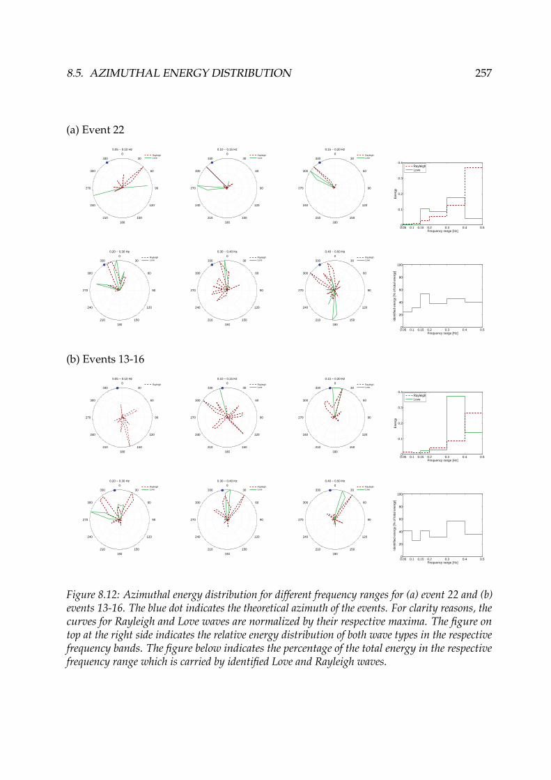
8.5. AZIMUTHAL ENERGY DISTRIBUTION 257

(a) Event 22

0

30

60

90

120

150

180

210

240

270

300

330

0.05 − 0.10 Hz

RayleighLove

0

30

60

90

120

150

180

210

240

270

300

330

0.10 − 0.15 Hz

RayleighLove

0

30

60

90

120

150

180

210

240

270

300

330

0.15 − 0.20 Hz

RayleighLove

0.05 0.1 0.15 0.2 0.3 0.4 0.50

0.1

0.2

0.3

0.4

Frequency range [Hz]

Ene

rgy

RayleighLove

0

30

60

90

120

150

180

210

240

270

300

330

0.20 − 0.30 Hz

RayleighLove

0

30

60

90

120

150

180

210

240

270

300

330

0.30 − 0.40 Hz

RayleighLove

0

30

60

90

120

150

180

210

240

270

300

330

0.40 − 0.50 Hz

RayleighLove

0.05 0.1 0.15 0.2 0.3 0.4 0.50

20

40

60

80

100

Frequency range [Hz]

Iden

tifie

d en

ergy

[% o

f tot

al e

nerg

y]

(b) Events 13-16

0

30

60

90

120

150

180

210

240

270

300

330

0.05 − 0.10 Hz

Rayleigh 0

30

60

90

120

150

180

210

240

270

300

330

0.10 − 0.15 Hz

RayleighLove

0

30

60

90

120

150

180

210

240

270

300

330

0.15 − 0.20 Hz

RayleighLove

0.05 0.1 0.15 0.2 0.3 0.4 0.50

0.1

0.2

0.3

0.4

Frequency range [Hz]

Ene

rgy

RayleighLove

0

30

60

90

120

150

180

210

240

270

300

330

0.20 − 0.30 Hz

RayleighLove

0

30

60

90

120

150

180

210

240

270

300

330

0.30 − 0.40 Hz

RayleighLove

0

30

60

90

120

150

180

210

240

270

300

330

0.40 − 0.50 Hz

RayleighLove

0.05 0.1 0.15 0.2 0.3 0.4 0.50

20

40

60

80

100

Frequency range [Hz]

Iden

tifie

d en

ergy

[% o

f tot

al e

nerg

y]

Figure 8.12: Azimuthal energy distribution for different frequency ranges for (a) event 22 and (b)events 13-16. The blue dot indicates the theoretical azimuth of the events. For clarity reasons, thecurves for Rayleigh and Love waves are normalized by their respective maxima. The figure ontop at the right side indicates the relative energy distribution of both wave types in the respectivefrequency bands. The figure below indicates the percentage of the total energy in the respectivefrequency range which is carried by identified Love and Rayleigh waves.

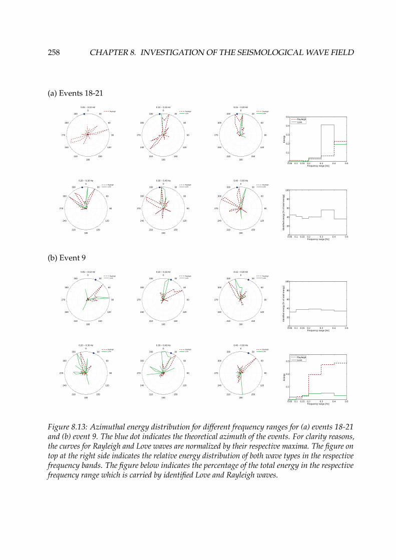
258 CHAPTER 8. INVESTIGATION OF THE SEISMOLOGICAL WAVE FIELD

(a) Events 18-21

0

30

60

90

120

150

180

210

240

270

300

330

0.05 − 0.10 Hz

Rayleigh 0

30

60

90

120

150

180

210

240

270

300

330

0.10 − 0.15 Hz

RayleighLove

0

30

60

90

120

150

180

210

240

270

300

330

0.15 − 0.20 Hz

RayleighLove

0.05 0.1 0.15 0.2 0.3 0.4 0.50

0.1

0.2

0.3

0.4

0.5

Frequency range [Hz]

Ene

rgy

RayleighLove

0

30

60

90

120

150

180

210

240

270

300

330

0.20 − 0.30 Hz

RayleighLove

0

30

60

90

120

150

180

210

240

270

300

330

0.30 − 0.40 Hz

RayleighLove

0

30

60

90

120

150

180

210

240

270

300

330

0.40 − 0.50 Hz

RayleighLove

0.05 0.1 0.15 0.2 0.3 0.4 0.50

20

40

60

80

100

Frequency range [Hz]

Iden

tifie

d en

ergy

[% o

f tot

al e

nerg

y]

(b) Event 9

0

30

60

90

120

150

180

210

240

270

300

330

0.05 − 0.10 Hz

RayleighLove

0

30

60

90

120

150

180

210

240

270

300

330

0.10 − 0.15 Hz

RayleighLove

0

30

60

90

120

150

180

210

240

270

300

330

0.15 − 0.20 Hz

RayleighLove

0.05 0.1 0.15 0.2 0.3 0.4 0.50

20

40

60

80

100

Frequency range [Hz]

Iden

tifie

d en

ergy

[% o

f tot

al e

nerg

y]

0

30

60

90

120

150

180

210

240

270

300

330

0.20 − 0.30 Hz

RayleighLove

0

30

60

90

120

150

180

210

240

270

300

330

0.30 − 0.40 Hz

RayleighLove

0

30

60

90

120

150

180

210

240

270

300

330

0.40 − 0.50 Hz

RayleighLove

0.05 0.1 0.15 0.2 0.3 0.4 0.50

0.1

0.2

0.3

Frequency range [Hz]

Ene

rgy

RayleighLove

Figure 8.13: Azimuthal energy distribution for different frequency ranges for (a) events 18-21and (b) event 9. The blue dot indicates the theoretical azimuth of the events. For clarity reasons,the curves for Rayleigh and Love waves are normalized by their respective maxima. The figure ontop at the right side indicates the relative energy distribution of both wave types in the respectivefrequency bands. The figure below indicates the percentage of the total energy in the respectivefrequency range which is carried by identified Love and Rayleigh waves.

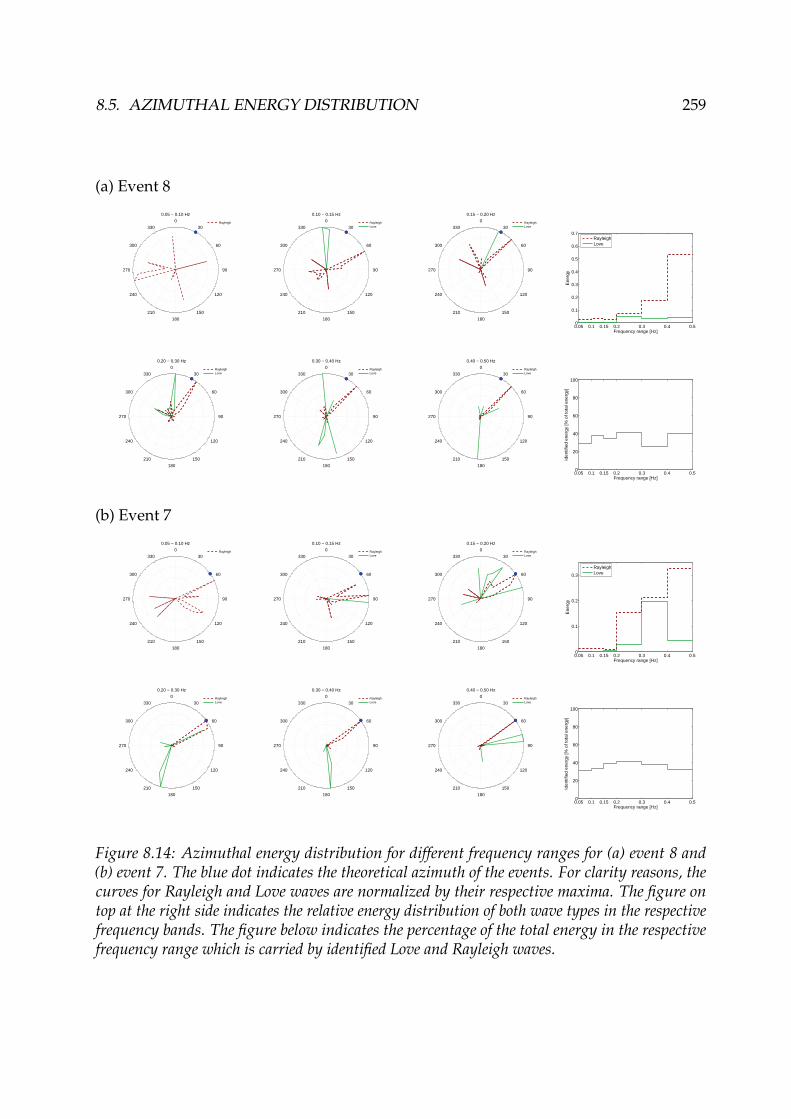
8.5. AZIMUTHAL ENERGY DISTRIBUTION 259

(a) Event 8

0

30

60

90

120

150

180

210

240

270

300

330

0.05 − 0.10 Hz

Rayleigh 0

30

60

90

120

150

180

210

240

270

300

330

0.10 − 0.15 Hz

RayleighLove

0

30

60

90

120

150

180

210

240

270

300

330

0.15 − 0.20 Hz

RayleighLove

0.05 0.1 0.15 0.2 0.3 0.4 0.50

0.1

0.2

0.3

0.4

0.5

0.6

0.7

Frequency range [Hz]

Ene

rgy

RayleighLove

0

30

60

90

120

150

180

210

240

270

300

330

0.20 − 0.30 Hz

RayleighLove

0

30

60

90

120

150

180

210

240

270

300

330

0.30 − 0.40 Hz

RayleighLove

0

30

60

90

120

150

180

210

240

270

300

330

0.40 − 0.50 Hz

RayleighLove

0.05 0.1 0.15 0.2 0.3 0.4 0.50

20

40

60

80

100

Frequency range [Hz]

Iden

tifie

d en

ergy

[% o

f tot

al e

nerg

y]

(b) Event 7

0

30

60

90

120

150

180

210

240

270

300

330

0.05 − 0.10 Hz

Rayleigh 0

30

60

90

120

150

180

210

240

270

300

330

0.10 − 0.15 Hz

RayleighLove

0

30

60

90

120

150

180

210

240

270

300

330

0.15 − 0.20 Hz

RayleighLove

0.05 0.1 0.15 0.2 0.3 0.4 0.50

0.1

0.2

0.3

Frequency range [Hz]

Ene

rgy

RayleighLove

0

30

60

90

120

150

180

210

240

270

300

330

0.20 − 0.30 Hz

RayleighLove

0

30

60

90

120

150

180

210

240

270

300

330

0.30 − 0.40 Hz

RayleighLove

0

30

60

90

120

150

180

210

240

270

300

330

0.40 − 0.50 Hz

RayleighLove

0.05 0.1 0.15 0.2 0.3 0.4 0.50

20

40

60

80

100

Frequency range [Hz]

Iden

tifie

d en

ergy

[% o

f tot

al e

nerg

y]

Figure 8.14: Azimuthal energy distribution for different frequency ranges for (a) event 8 and(b) event 7. The blue dot indicates the theoretical azimuth of the events. For clarity reasons, thecurves for Rayleigh and Love waves are normalized by their respective maxima. The figure ontop at the right side indicates the relative energy distribution of both wave types in the respectivefrequency bands. The figure below indicates the percentage of the total energy in the respectivefrequency range which is carried by identified Love and Rayleigh waves.

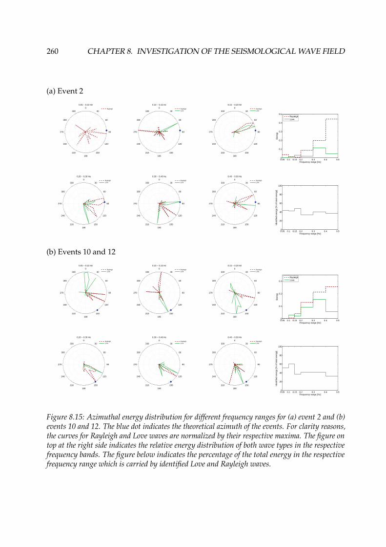
260 CHAPTER 8. INVESTIGATION OF THE SEISMOLOGICAL WAVE FIELD

(a) Event 2

0

30

60

90

120

150

180

210

240

270

300

330

0.05 − 0.10 Hz

Rayleigh 0

30

60

90

120

150

180

210

240

270

300

330

0.10 − 0.15 Hz

RayleighLove

0

30

60

90

120

150

180

210

240

270

300

330

0.15 − 0.20 Hz

RayleighLove

0.05 0.1 0.15 0.2 0.3 0.4 0.50

0.1

0.2

0.3

0.4

0.5

Frequency range [Hz]

Ene

rgy

RayleighLove

0

30

60

90

120

150

180

210

240

270

300

330

0.20 − 0.30 Hz

RayleighLove

0

30

60

90

120

150

180

210

240

270

300

330

0.30 − 0.40 Hz

RayleighLove

0

30

60

90

120

150

180

210

240

270

300

330

0.40 − 0.50 Hz

RayleighLove

0.05 0.1 0.15 0.2 0.3 0.4 0.50

20

40

60

80

100

Frequency range [Hz]

Iden

tifie

d en

ergy

[% o

f tot

al e

nerg

y]

(b) Events 10 and 12

0

30

60

90

120

150

180

210

240

270

300

330

0.05 − 0.10 Hz

RayleighLove

0

30

60

90

120

150

180

210

240

270

300

330

0.10 − 0.15 Hz

RayleighLove

0

30

60

90

120

150

180

210

240

270

300

330

0.15 − 0.20 Hz

RayleighLove

0.05 0.1 0.15 0.2 0.3 0.4 0.50

0.1

0.2

0.3

Frequency range [Hz]

Ene

rgy

RayleighLove

0

30

60

90

120

150

180

210

240

270

300

330

0.20 − 0.30 Hz

RayleighLove

0

30

60

90

120

150

180

210

240

270

300

330

0.30 − 0.40 Hz

RayleighLove

0

30

60

90

120

150

180

210

240

270

300

330

0.40 − 0.50 Hz

RayleighLove

0.05 0.1 0.15 0.2 0.3 0.4 0.50

20

40

60

80

100

Frequency range [Hz]

Iden

tifie

d en

ergy

[% o

f tot

al e

nerg

y]

Figure 8.15: Azimuthal energy distribution for different frequency ranges for (a) event 2 and (b)events 10 and 12. The blue dot indicates the theoretical azimuth of the events. For clarity reasons,the curves for Rayleigh and Love waves are normalized by their respective maxima. The figure ontop at the right side indicates the relative energy distribution of both wave types in the respectivefrequency bands. The figure below indicates the percentage of the total energy in the respectivefrequency range which is carried by identified Love and Rayleigh waves.

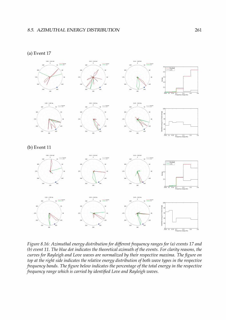
8.5. AZIMUTHAL ENERGY DISTRIBUTION 261

(a) Event 17

0

30

60

90

120

150

180

210

240

270

300

330

0.05 − 0.10 Hz

RayleighLove

0

30

60

90

120

150

180

210

240

270

300

330

0.10 − 0.15 Hz

RayleighLove

0

30

60

90

120

150

180

210

240

270

300

330

0.15 − 0.20 Hz

RayleighLove

0.05 0.1 0.15 0.2 0.3 0.4 0.50

0.1

0.2

0.3

0.4

0.5

Frequency range [Hz]

Ene

rgy

RayleighLove

0

30

60

90

120

150

180

210

240

270

300

330

0.20 − 0.30 Hz

RayleighLove

0

30

60

90

120

150

180

210

240

270

300

330

0.30 − 0.40 Hz

RayleighLove

0

30

60

90

120

150

180

210

240

270

300

330

0.40 − 0.50 Hz

RayleighLove

0.05 0.1 0.15 0.2 0.3 0.4 0.50

20

40

60

80

100

Frequency range [Hz]

Iden

tifie

d en

ergy

[% o

f tot

al e

nerg

y]

(b) Event 11

0

30

60

90

120

150

180

210

240

270

300

330

0.05 − 0.10 Hz

RayleighLove

0

30

60

90

120

150

180

210

240

270

300

330

0.10 − 0.15 Hz

RayleighLove

0

30

60

90

120

150

180

210

240

270

300

330

0.15 − 0.20 Hz

RayleighLove

0.05 0.1 0.15 0.2 0.3 0.4 0.50

0.1

0.2

0.3

Frequency range [Hz]

Ene

rgy

RayleighLove

0

30

60

90

120

150

180

210

240

270

300

330

0.20 − 0.30 Hz

RayleighLove

0

30

60

90

120

150

180

210

240

270

300

330

0.30 − 0.40 Hz

RayleighLove

0

30

60

90

120

150

180

210

240

270

300

330

0.40 − 0.50 Hz

RayleighLove

0.05 0.1 0.15 0.2 0.3 0.4 0.50

20

40

60

80

100

Frequency range [Hz]

Iden

tifie

d en

ergy

[% o

f tot

al e

nerg

y]

Figure 8.16: Azimuthal energy distribution for different frequency ranges for (a) events 17 and(b) event 11. The blue dot indicates the theoretical azimuth of the events. For clarity reasons, thecurves for Rayleigh and Love waves are normalized by their respective maxima. The figure ontop at the right side indicates the relative energy distribution of both wave types in the respectivefrequency bands. The figure below indicates the percentage of the total energy in the respectivefrequency range which is carried by identified Love and Rayleigh waves.

262 CHAPTER 8. INVESTIGATION OF THE SEISMOLOGICAL WAVE FIELD

8.6 Energy repartition between Love and Rayleigh waves

The energy repartition between the different surface wave types is given for each eventin table 8.2. The indicated energies are the total energies for all 50 analyzed frequenciesin the range between 0.05 and 0.50 Hz. We decided in the MUSIQUE code to identifythe signal of a time window as Love wave if the transverse energy in the respective timewindow is dominant. The Love wave energy indicated in the table corresponds to thesummed transverse energies of all time windows which have been attributed to Lovewaves. The radial and vertical energies of these windows are also included in the table.These latter energies correspond to the less energetic waves in the signal, which caninclude Love or Rayleigh waves arriving under different azimuths. The energy of these"wrong" components is, by construction of the method, always smaller than the energy ofthe components corresponding to the identified wave. For the values given in the table,in average, the energies not corresponding to the identified dominant wave type carryabout two-thirds of the energy corresponding to the identified wave type (i.e. in average,the radial and vertical components of the windows identified as Love waves carry about67 % of the energy of the respective transverse components). For the Rayleigh waves, thesignal energy is carried by the radial and vertical components, whereas the transversecomponent is composed by inferior wave contributions.The energy repartition between the different wave types varies largely for the differentevents. The proportion of Love waves ranges from 4.5 % (event 8) to 30.9 % (event 19),with an average of 17.4 %. The retrograde Rayleigh wave proportion is quite stable forthe different events, taking values from 7.0 to 12.8 %, whereas the prograde Rayleighwave proportion is more variable, accounting for 5.4 to 25.2 % of the energy. The un-classified waves contribute between 25.0 and 40.5 % to the total energy, but, in fact, alsothe contributions of the components not corresponding to the identified polarization ofeach time window are not attributed to a wave type. The energy repartition betweenclassified Love and Rayleigh waves is indicated in the table as well.The last column of the table indicates the proportion of Love wave energy which isarriving from the south (with azimuths between 150◦ and 210◦). This proportion is alsorepresented in function of the theoretical earthquake azimuth in figure 8.17. For eventslocated north of the array, this proportion ranges from 0 to 12.8 %. For events locatedin the north-east, the proportion is rather high, with values of 12.4 % (event 9), 30.1 %(event 8) and the highest proportion of all events is observed for event 7 with 76.8 % ofthe Love wave energy arriving from the south. For events located at the east, about 30 %of the Love wave energy comes from the south. Finally, for events located south-east ofthe array, 31.0 to 58.7 % of the Love wave energy is incident from southern directions.

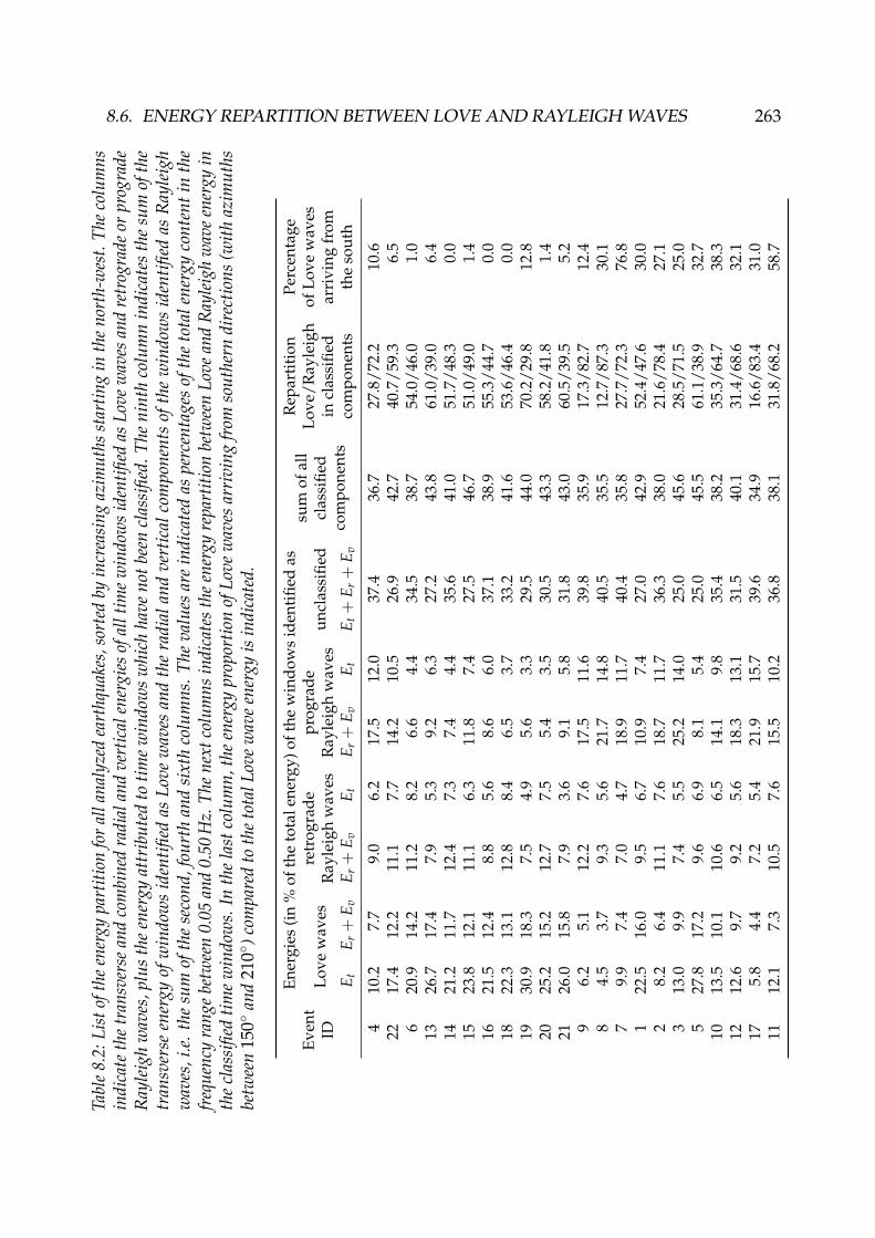
8.6. ENERGY REPARTITION BETWEEN LOVE AND RAYLEIGH WAVES 263Ta

ble

8.2:

List

ofth

een

ergy

part

ition

for

alla

naly

zed

eart

hqua

kes,

sort

edby

incr

easi

ngaz

imut

hsst

artin

gin

the

nort

h-w

est.

The

colu

mns

indi

cate

the

tran

sver

sean

dco

mbi

ned

radi

alan

dve

rtic

alen

ergi

esof

allt

ime

win

dow

sid

entifi

edas

Love

wav

esan

dre

trog

rade

orpr

ogra

deR

ayle

igh

wav

es,p

lus

the

ener

gyat

trib

uted

totim

ew

indo

ws

whi

chha

veno

tbee

ncl

assi

fied.

The

nint

hco

lum

nin

dica

tes

the

sum

ofth

etr

ansv

erse

ener

gyof

win

dow

sid

enti

fied

asLo

vew

aves

and

the

radi

alan

dve

rtic

alco

mpo

nent

sof

the

win

dow

sid

enti

fied

asR

ayle

igh

wav

es,i

.e.t

hesu

mof

the

seco

nd,f

ourt

han

dsi

xth

colu

mns

.The

valu

esar

ein

dica

ted

aspe

rcen

tage

sof

the

tota

lene

rgy

cont

enti

nth

efr

eque

ncy

rang

ebe

twee

n0.

05an

d0.

50H

z.Th

ene

xtco

lum

nsin

dica

tes

the

ener

gyre

part

ition

betw

een

Love

and

Ray

leig

hw

ave

ener

gyin

the

clas

sifie

dtim

ew

indo

ws.

Inth

ela

stco

lum

n,th

een

ergy

prop

ortio

nof

Love

wav

esar

rivi

ngfr

omso

uthe

rndi

rect

ions

(with

azim

uths

betw

een

150◦

and

210◦

)com

pare

dto

the

tota

lLov

ew

ave

ener

gyis

indi

cate

d.

Ener

gies

(in

%of

the

tota

lene

rgy)

ofth

ew

indo

ws

iden

tifie

das

Rep

arti

tion

Perc

enta

geEv

ent

retr

ogra

depr

ogra

desu

mof

all

Love

/Ray

leig

hof

Love

wav

esID

Love

wav

esR

ayle

igh

wav

esR

ayle

igh

wav

esun

clas

sifie

dcl

assi

fied

incl

assi

fied

arri

ving

from

E tE r

+E v

E r+

E vE t

E r+

E vE t

E t+

E r+

E vco

mpo

nent

sco

mpo

nent

sth

eso

uth

410

.27.

79.

06.

217

.512

.037

.436

.727

.8/

72.2

10.6

2217

.412

.211

.17.

714

.210

.526

.942

.740

.7/

59.3

6.5

620

.914

.211

.28.

26.

64.

434

.538

.754

.0/

46.0

1.0

1326

.717

.47.

95.

39.

26.

327

.243

.861

.0/

39.0

6.4

1421

.211

.712

.47.

37.

44.

435

.641

.051

.7/

48.3

0.0

1523

.812

.111

.16.

311

.87.

427

.546

.751

.0/

49.0

1.4

1621

.512

.48.

85.

68.

66.

037

.138

.955

.3/

44.7

0.0

1822

.313

.112

.88.

46.

53.

733

.241

.653

.6/

46.4

0.0

1930

.918

.37.

54.

95.

63.

329

.544

.070

.2/

29.8

12.8

2025

.215

.212

.77.

55.

43.

530

.543

.358

.2/

41.8

1.4

2126

.015

.87.

93.

69.

15.

831

.843

.060

.5/

39.5

5.2

96.

25.

112

.27.

617

.511

.639

.835

.917

.3/

82.7

12.4

84.

53.

79.

35.

621

.714

.840

.535

.512

.7/

87.3

30.1

79.

97.

47.

04.

718

.911

.740

.435

.827

.7/

72.3

76.8

122

.516

.09.

56.

710

.97.

427

.042

.952

.4/

47.6

30.0

28.

26.

411

.17.

618

.711

.736

.338

.021

.6/

78.4

27.1

313

.09.

97.

45.

525

.214

.025

.045

.628

.5/

71.5

25.0

527

.817

.29.

66.

98.

15.

425

.045

.561

.1/

38.9

32.7

1013

.510

.110

.66.

514

.19.

835

.438

.235

.3/

64.7

38.3

1212

.69.

79.

25.

618

.313

.131

.540

.131

.4/

68.6

32.1

175.

84.

47.

25.

421

.915

.739

.634

.916

.6/

83.4

31.0

1112

.17.

310

.57.

615

.510

.236

.838

.131

.8/

68.2

58.7

264 CHAPTER 8. INVESTIGATION OF THE SEISMOLOGICAL WAVE FIELD

300 0 60 120 1800

20

40

60

80

Love

wav

es a

rriv

ing

from

the

sout

h [%

]

Azimuth [°]

Figure 8.17: Proportion of Love wave energy arriving from southern directions (azimuths between150◦ and 210◦) in function of the theoretical azimuth for all analyzed earthquakes.

In figure 8.18, the energy repartition between Love, retrograde and prograde Rayleighwaves is shown in different frequency ranges for all analyzed events. Some events whichare closely located and exhibit similar behavior have been grouped together for clarityreasons. A strong peak of the Love wave energy can be seen for frequencies between0.15 and 0.20 Hz for all events except event 5 and the group of events 18-21. For event5, the strongest magnitude event in the dataset, however, the Love wave energy is verystrong in the whole low-frequency range. The two groups of events 13-16 and 18-21both show very energetic Love waves between 0.3 and 0.4 Hz. With distances of 44 kmand 42 km, respectively, these events are the closest to the array. For the other events, itmight be that Love waves have been generated in this frequency range, but are alreadyattenuated when arriving at the array. Nevertheless, a smaller Love wave energy peakat these frequencies can be seen for events 22, 6, 7, 1 and 2, which are all located underazimuths between 329◦ and 86◦.For retrograde Rayleigh waves, no specific behavior can be observed, for some eventsthe energy content is almost constant with frequency (events 13-16, 3 and 5), while forother events the amount of energy changes strongly with frequency (e.g. events 4, 18-21,7), without following a systematic scheme.Prograde Rayleigh waves are strongest at higher frequencies for most events. Accordingto the basin model, the fundamental Rayleigh wave mode is retrograde at all frequencies.Therefore, prograde Rayleigh waves correspond to the first harmonic mode, whichdoes not exist below 0.17 Hz. Consequently, prograde Rayleigh waves found at lowerfrequencies are probably misidentified. The peak of prograde Rayleigh waves observedfor events 18-21 in the range between 0.15 and 0.20 Hz is not visible for other events.

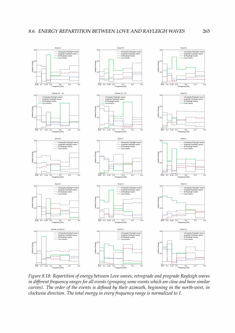
8.6. ENERGY REPARTITION BETWEEN LOVE AND RAYLEIGH WAVES 265

0.05 0.1 0.15 0.2 0.3 0.4 0.50

0.2

0.4

0.6

Frequency [Hz]

rela

tive

Ene

rgy

Event 4

retrograde Rayleigh wavesprograde Rayleigh wavesall Rayleigh wavesLove waves

0.05 0.1 0.15 0.2 0.3 0.4 0.50

0.2

0.4

0.6

Frequency [Hz]

rela

tive

Ene

rgy

Event 22

retrograde Rayleigh wavesprograde Rayleigh wavesall Rayleigh wavesLove waves

0.05 0.1 0.15 0.2 0.3 0.4 0.50

0.2

0.4

0.6

Frequency [Hz]

rela

tive

Ene

rgy

Event 6

retrograde Rayleigh wavesprograde Rayleigh wavesall Rayleigh wavesLove waves

0.05 0.1 0.15 0.2 0.3 0.4 0.50

0.2

0.4

0.6

Frequency [Hz]

rela

tive

Ene

rgy

Events 13 − 16

retrograde Rayleigh wavesprograde Rayleigh wavesall Rayleigh wavesLove waves

0.05 0.1 0.15 0.2 0.3 0.4 0.50

0.2

0.4

0.6

Frequency [Hz]

rela

tive

Ene

rgy

Events 18 − 21

retrograde Rayleigh wavesprograde Rayleigh wavesall Rayleigh wavesLove waves

0.05 0.1 0.15 0.2 0.3 0.4 0.50

0.2

0.4

0.6

Frequency [Hz]

rela

tive

Ene

rgy

Event 9

retrograde Rayleigh wavesprograde Rayleigh wavesall Rayleigh wavesLove waves

0.05 0.1 0.15 0.2 0.3 0.4 0.50

0.2

0.4

0.6

Frequency [Hz]

rela

tive

Ene

rgy

Event 8

retrograde Rayleigh wavesprograde Rayleigh wavesall Rayleigh wavesLove waves

0.05 0.1 0.15 0.2 0.3 0.4 0.50

0.2

0.4

0.6

Frequency [Hz]

rela

tive

Ene

rgy

Event 7

retrograde Rayleigh wavesprograde Rayleigh wavesall Rayleigh wavesLove waves

0.05 0.1 0.15 0.2 0.3 0.4 0.50

0.2

0.4

0.6

Frequency [Hz]

rela

tive

Ene

rgy

Event 1

retrograde Rayleigh wavesprograde Rayleigh wavesall Rayleigh wavesLove waves

0.05 0.1 0.15 0.2 0.3 0.4 0.50

0.2

0.4

0.6

Frequency [Hz]

rela

tive

Ene

rgy

Event 2

retrograde Rayleigh wavesprograde Rayleigh wavesall Rayleigh wavesLove waves

0.05 0.1 0.15 0.2 0.3 0.4 0.50

0.2

0.4

0.6

Frequency [Hz]

rela

tive

Ene

rgy

Event 3

retrograde Rayleigh wavesprograde Rayleigh wavesall Rayleigh wavesLove waves

0.05 0.1 0.15 0.2 0.3 0.4 0.50

0.2

0.4

0.6

Frequency [Hz]

rela

tive

Ene

rgy

Event 5

retrograde Rayleigh wavesprograde Rayleigh wavesall Rayleigh wavesLove waves

0.05 0.1 0.15 0.2 0.3 0.4 0.50

0.2

0.4

0.6

Frequency [Hz]

rela

tive

Ene

rgy

Events 10 and 12

retrograde Rayleigh wavesprograde Rayleigh wavesall Rayleigh wavesLove waves

0.05 0.1 0.15 0.2 0.3 0.4 0.50

0.2

0.4

0.6

Frequency [Hz]

rela

tive

Ene

rgy

Event 17

retrograde Rayleigh wavesprograde Rayleigh wavesall Rayleigh wavesLove waves

0.05 0.1 0.15 0.2 0.3 0.4 0.50

0.2

0.4

0.6

Frequency [Hz]

rela

tive

Ene

rgy

Event 11

retrograde Rayleigh wavesprograde Rayleigh wavesall Rayleigh wavesLove waves

Figure 8.18: Repartition of energy between Love waves, retrograde and prograde Rayleigh wavesin different frequency ranges for all events (grouping some events which are close and have similarcurves). The order of the events is defined by their azimuth, beginning in the north-west, inclockwise direction. The total energy in every frequency range is normalized to 1.

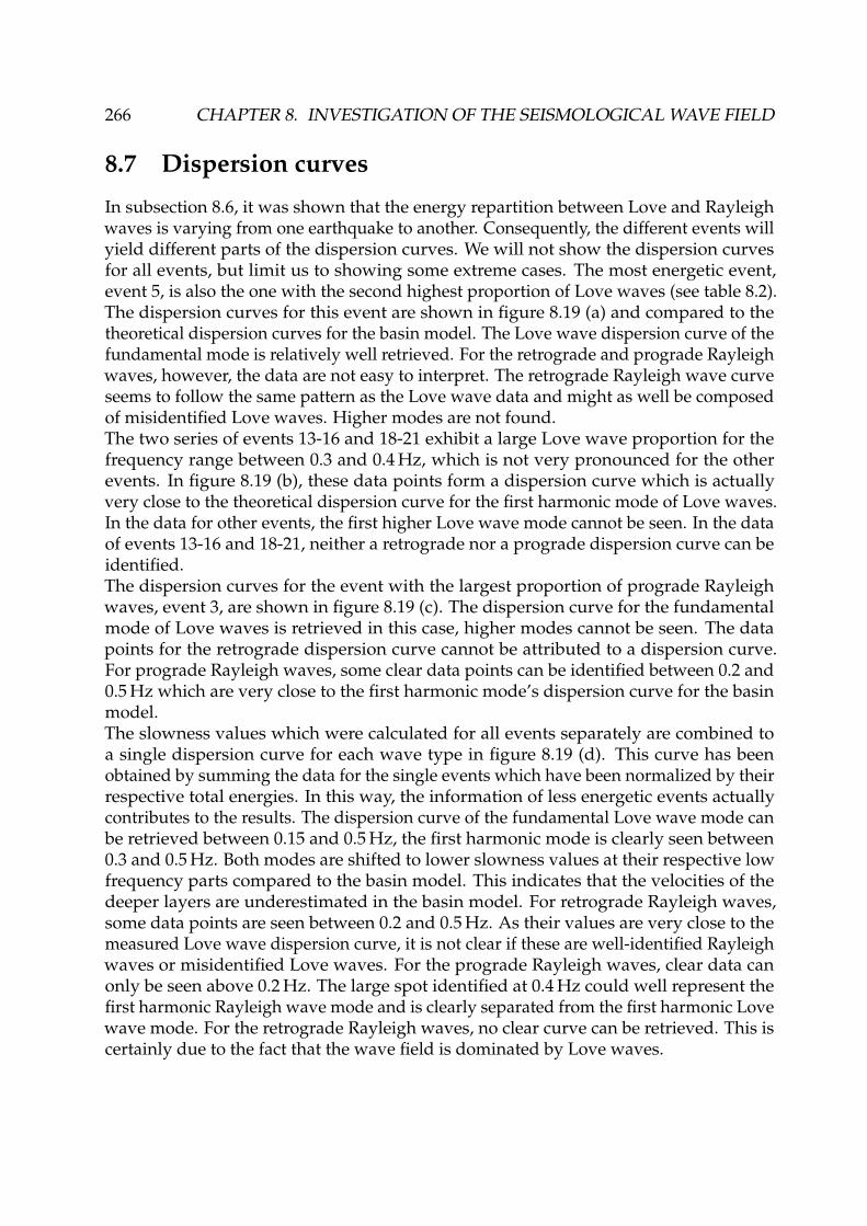
266 CHAPTER 8. INVESTIGATION OF THE SEISMOLOGICAL WAVE FIELD

8.7 Dispersion curves

In subsection 8.6, it was shown that the energy repartition between Love and Rayleighwaves is varying from one earthquake to another. Consequently, the different events willyield different parts of the dispersion curves. We will not show the dispersion curvesfor all events, but limit us to showing some extreme cases. The most energetic event,event 5, is also the one with the second highest proportion of Love waves (see table 8.2).The dispersion curves for this event are shown in figure 8.19 (a) and compared to thetheoretical dispersion curves for the basin model. The Love wave dispersion curve of thefundamental mode is relatively well retrieved. For the retrograde and prograde Rayleighwaves, however, the data are not easy to interpret. The retrograde Rayleigh wave curveseems to follow the same pattern as the Love wave data and might as well be composedof misidentified Love waves. Higher modes are not found.The two series of events 13-16 and 18-21 exhibit a large Love wave proportion for thefrequency range between 0.3 and 0.4 Hz, which is not very pronounced for the otherevents. In figure 8.19 (b), these data points form a dispersion curve which is actuallyvery close to the theoretical dispersion curve for the first harmonic mode of Love waves.In the data for other events, the first higher Love wave mode cannot be seen. In the dataof events 13-16 and 18-21, neither a retrograde nor a prograde dispersion curve can beidentified.The dispersion curves for the event with the largest proportion of prograde Rayleighwaves, event 3, are shown in figure 8.19 (c). The dispersion curve for the fundamentalmode of Love waves is retrieved in this case, higher modes cannot be seen. The datapoints for the retrograde dispersion curve cannot be attributed to a dispersion curve.For prograde Rayleigh waves, some clear data points can be identified between 0.2 and0.5 Hz which are very close to the first harmonic mode’s dispersion curve for the basinmodel.The slowness values which were calculated for all events separately are combined toa single dispersion curve for each wave type in figure 8.19 (d). This curve has beenobtained by summing the data for the single events which have been normalized by theirrespective total energies. In this way, the information of less energetic events actuallycontributes to the results. The dispersion curve of the fundamental Love wave mode canbe retrieved between 0.15 and 0.5 Hz, the first harmonic mode is clearly seen between0.3 and 0.5 Hz. Both modes are shifted to lower slowness values at their respective lowfrequency parts compared to the basin model. This indicates that the velocities of thedeeper layers are underestimated in the basin model. For retrograde Rayleigh waves,some data points are seen between 0.2 and 0.5 Hz. As their values are very close to themeasured Love wave dispersion curve, it is not clear if these are well-identified Rayleighwaves or misidentified Love waves. For the prograde Rayleigh waves, clear data canonly be seen above 0.2 Hz. The large spot identified at 0.4 Hz could well represent thefirst harmonic Rayleigh wave mode and is clearly separated from the first harmonic Lovewave mode. For the retrograde Rayleigh waves, no clear curve can be retrieved. This iscertainly due to the fact that the wave field is dominated by Love waves.

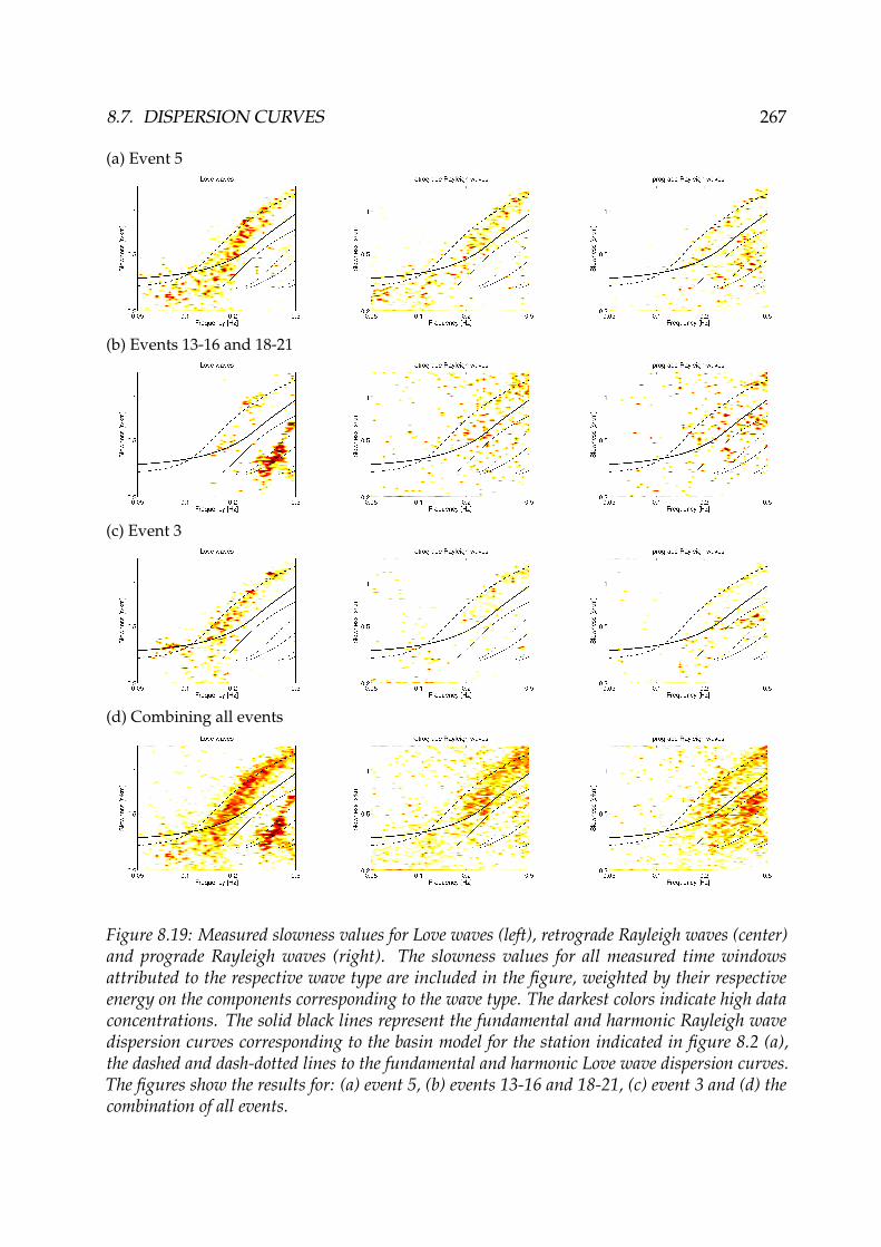
8.7. DISPERSION CURVES 267

(a) Event 5

(b) Events 13-16 and 18-21

(c) Event 3

(d) Combining all events

Figure 8.19: Measured slowness values for Love waves (left), retrograde Rayleigh waves (center)and prograde Rayleigh waves (right). The slowness values for all measured time windowsattributed to the respective wave type are included in the figure, weighted by their respectiveenergy on the components corresponding to the wave type. The darkest colors indicate high dataconcentrations. The solid black lines represent the fundamental and harmonic Rayleigh wavedispersion curves corresponding to the basin model for the station indicated in figure 8.2 (a),the dashed and dash-dotted lines to the fundamental and harmonic Love wave dispersion curves.The figures show the results for: (a) event 5, (b) events 13-16 and 18-21, (c) event 3 and (d) thecombination of all events.

268 CHAPTER 8. INVESTIGATION OF THE SEISMOLOGICAL WAVE FIELD

An alternative way of analyzing the data without taking Love waves into account is to usethe vertical component of the signals only. However, the polarization characteristics ofthe waves, i.e. the retrograde or prograde sense of motion as well as the ellipticity, cannotbe retrieved in this case. Figure 8.20 (a) shows the combination of the retrograde andprograde Rayleigh wave dispersion curves of figure 8.19 (d). The resulting dispersioncurve which is obtained by averaging the results of analyzing the vertical component ofthe signal only for all events is shown in figure 8.20 (b). The data form a large cloud ofpoints which spans the theoretical dispersion curves for the basin model’s fundamentaland first harmonic Rayleigh wave modes. It cannot be determined to which mode thedata points correspond or if they correspond to a mixture of both modes. However, thecloud of points is clearly distinguished from the Love wave dispersion curve measuredin figure 8.19 (d). This suggests that the retrograde Rayleigh wave dispersion curve offigure 8.19 (d) is actually biased by Love waves. Nevertheless, the prograde Rayleighwave of figure 8.19 (d) is not retrieved in figure 8.20 (b) either. It might be masked by thelarge cloud of points or be biased to lower slowness values by the harmonic Love wavemode.

(a) (b)

Figure 8.20: Measured slowness values for both Rayleigh wave types, averaged for all events.The slowness values for all measured time windows attributed to Rayleigh waves are includedin the figure, weighted by their respective energy on the radial and vertical components. Thedarkest colors indicate high data concentrations. The solid black lines represent the fundamentaland harmonic Rayleigh wave dispersion curves corresponding to the basin model for the stationindicated in figure 8.2 (a), the dashed and dash-dotted lines to the fundamental and harmonicLove wave dispersion curves. (a) shows the combination of the results for retrograde and progradeRayleigh waves shown in figure 8.19 (d). (b) was obtained analyzing the vertical componentsonly and thus eliminating any Love wave contributions.

8.8. ELLIPTICITY CURVES 269

8.8 Ellipticity curves

The ellipticity curves estimated by MUSIQUE using the results of all events togetherare shown in figure 8.21 for retrograde and prograde Rayleigh waves. The retrogradeellipticity curve is badly estimated and no ellipticity curve can be identified. For theprograde Rayleigh waves, a scattered ellipticity curve is retrieved, which can be at-tributed to the first harmonic mode. Below about 0.18 Hz, very few prograde waves areidentified compared to the higher frequency part. According to the basin model, the firstharmonic mode does not exist below 0.17 Hz. Actually, the retrieved ellipticity valuesare in good agreement with the first harmonic mode. This is a further indication thatthe fundamental mode does not exhibit a singularity. If such a singularity existed, themotion of the fundamental mode Rayleigh waves would be prograde for the frequenciesof the right flank of the peak, which would certainly bias the ellipticity estimation of thefirst harmonic mode.

Figure 8.21: Measured ellipticity values for retrograde Rayleigh waves (left) and progradeRayleigh waves (right) for considering all events together. The ellipticity values for all measuredtime windows attributed to the respective wave type are included in the figure, weighted by theirrespective amplitude. The darkest colors indicate high data concentrations. The solid black linerepresents the ellipticity curve of the fundamental mode and the dashed line of the first harmonicmode of Rayleigh waves corresponding to the basin model for the station indicated in figure 8.2(a).

270 CHAPTER 8. INVESTIGATION OF THE SEISMOLOGICAL WAVE FIELD

As it is based on statistics, a direct application of RayDec on earthquake signals would notmake sense because large energy arrivals which do not consist of Rayleigh waves couldnever be compensated. However, for event 5, the recording length of 22 minutes allowsthe application of the method to the late signal (see figure 8.5). We used the last sevenminutes of signal (starting 900 seconds after the signal beginning). The results of applyingRayDec, DELFI and H/V to this signal are shown in figure 8.22. The ellipticity curveestimations are rather instable, showing many little peaks for all methods. Nevertheless,the results suggest lower peak frequencies than predicted by the basin model. Thismodel predicts a value of 0.20 Hz, whereas RayDec and DELFI find a value of 0.18 Hzand H/V a value of 0.16 Hz. However, the signal is still quite short for an analysis at suchlow frequencies and the signal energy is still decreasing over the whole signal duration.At least RayDec supposes the signal amplitude to be quite stationary in time, which isnot the case here. Furthermore, the presence of the first harmonic Rayleigh wave modeabove 0.17 Hz is supposed to bias the estimation of the fundamental mode’s ellipticity.The three methods used here, however, are not able to distinguish between retrogradeand prograde waves or different modes and will yield a mixed estimation if more than asingle mode are present.

0.05 0.1 0.2 0.5

1

10

Frequency [Hz]

Elli

ptic

ity

basin model, fundamental modebasin model, first harmonic modeRayDecDELFIH/V

Figure 8.22: Ellipticity curves measured on the late signal of event 5 (seconds 900 to 1317) usingRayDec, DELFI and H/V.

8.9. CONCLUSION 271

8.9 Conclusion

This study investigated the seismological wave field generated by regional earthquakesin the Evergreen Basin, California, using MUSIQUE. In addition to the determination ofwave azimuth and velocity, the technique allows the identification of Love, retrogradeand prograde Rayleigh waves. The basin response to an earthquake depends on thelocation of the event. The azimuthal energy distribution is clearly different for wavesincident from north-western or south-eastern directions. In both cases, the energy at thearray is almost exclusively arriving from the respective hemicycle, with an importantexception. A large part of the Love wave energy arrives from the south, even for northernearthquakes. The extreme case is event 7, for which over 75 % of Love waves arrive fromthe south, i.e. an azimuth which is about 120◦ different from the direct connecting line.Frankel et al. [2001] already found evidence for a large Love wave scatterer located southof the array and attributed it either to a rock formation or to the southern basin edge.Apart from these southern Love waves, Love waves arrive under azimuths which areslightly deviated from the theoretical earthquake azimuths. The deviations are likelyto be explained by refraction of incident waves at the lateral borders of the basin. Ingeneral, we find that Rayleigh waves are more scattered and arrive under a multitude ofdifferent azimuths. As a detailed model of the San Francisco Bay Area exists, numericalsimulations could help to better understand the propagation patterns and to identify themost important wave scatterers.By analyzing the energy partition between Love and Rayleigh waves, we found largedifferences between the different earthquakes. The attributed Love wave energy rangesfrom about 5 to 30 %, whereas the retrograde Rayleigh wave energy is quite stable, takingvalues between 7 and 13 %. Between 5 and 25 % of the energy have been attributed toprograde Rayleigh waves, the total attributed energy constituting about 40 % of the totalsignal energy for all events. We identify prograde Rayleigh waves as the first harmonicmode. For the events located the closest to the array (about 40 km), the first harmonicLove wave mode can be found. For the other events, no such waves of significantamplitude can be identified. They might be produced as well during these earthquakes,but attenuated on their way to the array or this might be a feature attributed to thespecial location of these earthquakes.By combining the information of all earthquakes, we succeeded in retrieving the Lovewave dispersion curves for the fundamental and the first higher mode. The dispersioncurve found for retrograde Rayleigh waves is very close to the measured Love wavedispersion curve and could be biased by Love waves as well, particularly becausethe curve is completely different from the curve obtained by analyzing the verticalcomponents of the signal only. Furthermore, no ellipticity curve is found for these waves.For prograde Rayleigh waves, however, it is possible to identify the dispersion curveand assign an ellipticity curve.The inter-sensor spacing of the array limits the upper frequency limit of our analysis.Furthermore, the structure of the basin is not homogeneous under the total array size.Therefore, a smaller, but denser array located in the central part of the array would allowthe study of the higher-frequency part of incident waves. This might help to increase theunderstanding of the mechanisms of the Santa Clara Valley.

272 CHAPTER 8. INVESTIGATION OF THE SEISMOLOGICAL WAVE FIELD

AcknowledgmentsWe would like to thank Arthur Frankel and David Carver for kindly providing the dataand Arthur Rodgers for supplying the data of the San Francisco Bay Area model and forfruitful discussions.

Conclusion

Ellipticity measurement and inversion using single-station methodsA part of this work focused on the development of new methods allowing the charac-terization of surface waves. Two methods, DELFI and RayDec, have been designed toestimate the ellipticity of Rayleigh waves from single-sensor measurements.The first method, DELFI, tries to retrieve this property by fitting ellipses to parts of thesignal. If Rayleigh and Love waves are well separated in the signal, the method givesreliable results. However, if both wave types are present in the signal at the same time,the Love wave contributions lead to a misestimation of the ellipticity.The second method, RayDec, uses statistical properties to suppress other wave typesthan Rayleigh waves. The technique is especially adapted for the application to ambientseismic vibration measurements.

Ellipticity inversionThe ellipticity curve can be inverted in order to retrieve the local soil structure (i.e.the S-wave velocity profile). However, as the ellipticity function is not unambigious,additional information has to be included in the inversion process, e.g. small-scale SPACmeasurements or MASW measurements. The requirements and limits for such inversionshave been investigated for theoretical data. The main results are that the right flank ofthe ellipticity peak and the peak frequency itself carry all important information on thestructure. The left flank can be included in the inversion to better fix the peak frequency.The actual velocity values can be fixed both by SPAC or MASW measurements, but thefrequency range of this additional information should be close to the frequency range ofthe ellipticity curve used for inversion. Furthermore, it was shown that the errors on thesoil structure model induced by a misestimation of the ellipticity curve are about halfthe original misestimation. Nevertheless, the soil structure can only be retrieved downto the bedrock depth, as the absolute value of the shear wave velocity in the bedrock isbadly constrained.

Application to real data setsThe inversion scheme developed using the theoretical data has then been applied tomeasurements of ambient seismic vibrations performed during the European NERIESproject (2006-2010), where RayDec was used to measure the ellipticity. The results for 14different well-known sites, for which borehole measurements exist, show that the jointinversion of ellipticity and small-scale SPAC data are in good agreement with broad-banddispersion curve measurements.

275

276 CONCLUSION

No significant differences between the use of SPAC including larger (up to 8) or smaller(down to 3) numbers of sensors could be found. In this way, our method presentsan easier and cheaper way for the investigation of the soil structure than using arraynoise measurements. For some sites, the directly measured dispersion curves are indisagreement with the fundamental Rayleigh wave mode of the models obtained byellipticity inversion, but in good agreement with the first or second harmonic modesfor the same models. Considering the measured dispersion curve alone, however, itis difficult to decide which mode is actually measured. In these cases, an ellipticityinversion can help in identifying the correct mode. Another result of the analysis isthat, at least for soft sites, the Vs30 parameter obtained by joint ellipticity inversionsis in agreement with borehole measurements and can be helpful for seismic hazardassessment.

Investigation of wave field polarization parameters

MUSIQUEThe third method developed during this thesis work, MUSIQUE, is the combinationof two different MUSIC algorithms. The first algorithm, "classical" MUSIC, is a well-established method which has already been successfully applied to seismic measure-ments. The second algorithm, quaternion-MUSIC, is a rather new development in signalprocessing and has never been applied to real seismic data before. This code is limitedto two-component signals. Certainly, the use of quaternions increases the mathematicaland computational complexity of the method, but it allows the simultaneous use oftwo components and therefore the estimation of the polarization between these twocomponents. This finally extends the field of possible applications of array techniquesby discriminating between Love and Rayleigh waves. The additional benefit of usingquaternion-MUSIC is the identification of the retrograde or prograde sense of motionand the estimation of ellipticity. In this way, MUSIQUE estimates the contributions ofLove and Rayleigh waves to the wave field and characterizes the respective properties.

Biquaternion-MUSICA further aspect of the work was linked to biquaternion-MUSIC, an even more complexmethod which could, in theory, be applied to four-dimensional signals. Therefore, usingthis method, the three components of the seismic signal could be processed togetherin order to retrieve their respective polarization properties. Nevertheless, we foundthat the method cannot work in simple special cases, e.g. a purely two-dimensionalsignal. Modifications to the code might improve its performances and make the methodapplicable to complex real data measurements. However, each type of seismic wavesis always confined to a maximum of two different directions and can be characterizedusing quaternion-MUSIC.

CONCLUSION 277

Application of MUSIQUEIn tests on synthetic seismic data, MUSIQUE proved its ability to separate not only Lovefrom Rayleigh waves, but also retrograde from prograde Rayleigh waves. Furthermore,the respective ellipticities have been well retrieved.The application of MUSIQUE to seismological data measured by a dense accelerom-eter array located in the Santa Clara Valley, California, identified wave types whichcontributed about 40 % to the total signal energy. The diffracted surface wave field isespecially dominated by Love waves generated at the southern valley edge. Combin-ing all earthquakes, the dispersion curves of the fundamental and first harmonic Lovewave modes could be retrieved. Although it was possible to identify the dispersionand ellipticity curves of the first harmonic Rayleigh wave mode, the phase velocityestimations of the fundamental Rayleigh wave mode seem to be largely contaminated byLove wave contributions. Nevertheless, this data set appeared not to be the best suitedfor testing all the potentials of MUSIQUE because the fundamental Rayleigh wave modedoes not exhibit a singularity and therefore does not change its sense of motion. In thissense, this site cannot be considered as a school test site for the method. Furthermore,the analysis is restricted to a limited frequency range due to the array geometry. Anapplication of the method to other dense seismic array measurements might fully exploitall of its capabilities. The potential of the method might be fully tested by applying it tosimulations of the propagation of seismic waves in sediment-filled basins.

Perspectives

The joint inversion of ellipticity curves as presented in this work is a very promisingtechnique. However, further tests are needed to proof its applicability to seismic hazardassessment at sites for which noise data are already available (e.g. Beirut, alpine valleys).

A possible perspective of analyzing array measurements using MUSIQUE could be theapplication to other sites, but the number of available array measurements of high qualitywith a small enough array size is limited. Nevertheless, the method could be furthertested on synthetic signals generated for precise basin simulations as the San FranciscoBay Area model, the Euroseistest site in Volvi, Greece, or the Grenoble basin in France.A main objective of such investigations would consist in identifying if a systematiccorrelation between structure properties as the basin geometry or velocity profiles andthe wave type, i.e. Love and Rayleigh wave, exists.

Furthermore, it should be possible to still improve the method so that more than thedominant wave can be identified. Such an algorithm could for example be composed bya first identification of the dominant wave, followed by a subtraction of the respectivesignal from the recordings. Then, the properties of the second wave could be estimated,again followed by a subtraction of the respective signal and so on. Of course, misestima-tions in the different algorithm steps would accumulate for the weaker signal parts, butthis way of doing should allow the identification of the main wave contributions.

CONCLUSION 279

Mesures d’ellipticité à l’aide de méthodes monocapteurs et inversion

Une partie de ce manuscrit était centrée sur le développement de nouvelles méthodes permettantla caractérisation d’ondes de surface. Deux méthodes, DELFI et RayDec, ont été conçues pourestimer l’ellipticité d’ondes de Rayleigh à partir d’enregistrements d’un seul capteur.La première méthode, DELFI, cherche à retrouver cette propriété en ajustant des ellipses à desparties du signal. Si les ondes de Love et les ondes de Rayleigh sont bien séparées dans le signal,cette méthode donne des résultats fiables. Cependant, si les deux types d’ondes coexistenten même temps, les contributions des ondes de Love engendrent une mauvaise estimation del’ellipticité.La deuxième méthode, RayDec, profite de propriétés statistiques pour supprimer les ondes qui nesont pas des ondes de Rayleigh. La technique est particulièrement adaptée aux enregistrementsde vibrations sismiques ambiantes.

Inversion d’ellipticitéUne courbe d’ellipticité peut être inversée afin de retrouver la structure locale du sol (c’est-à-direle profil de vitesse des ondes de cisaillement). Comme l’ellipticité n’est pas une fonction unique,des informations complémentaires doivent être inclues dans l’inversion, par exemple des mesuresSPAC ou MASW pour contraindre les vitesses en surface. Les conditions et limites de cesinversions ont été évaluées pour des données théoriques. Les résultats principaux sont que leflanc droit du pic d’ellipticité et la fréquence du pic elle-même comportent toutes les informationsnécessaires sur la structure. Le flanc gauche du pic, quant à lui, peut être utilisé dans l’inversionpour mieux fixer la fréquence du pic. Les valeurs de vitesse réelles peuvent être fixées soit pardes données de mesures SPAC, soit par des mesures MASW, mais les bandes de fréquence deces informations complémentaires doivent être proches des gammes de fréquence de la courbed’ellipticité inversée. En plus, il a été montré que les erreurs sur la structure du sol induits pardes erreurs d’estimation de la courbe d’ellipticité ne représentent qu’à peu près la moitié del’erreur d’estimation originale. Quoi qu’il en soit, la structure du sol ne peut être retrouvé quejusqu’à la profondeur du bedrock, les valeurs absolues de la vitesse des ondes de cisaillementdans le bedrock étant mal contraintes.

280 CONCLUSION

Application aux données réellesLe schéma d’inversion développé à l’aide des données théoriques a ensuite été appliqué à desmesures de vibrations sismiques ambiantes effectuées dans le cadre du projet européen NERIES(2006-2010), utilisant RayDec pour mesurer les courbes d’ellipticité. Les résultats pour 14 sitesbien connus, où des mesures de référence par méthode en forage existent, montrent que lesinversions conjointes de courbes d’ellipticité et de courbes SPAC à petite échelle sont en bonaccord avec des mesures de dispersion large-bande. En plus, aucune différence significative entrel’utilisation d’un plus grand nombre (jusqu’à 8) ou d’un plus petit nombre (jusqu’à 3) de capteurspour les mesures SPAC n’a pu être identifiée. Notre méthode d’inversion représente donc unealternative plus simple et moins coûteuse pour estimer la structure en vitesse que des mesurespar réseaux. Pour quelques sites, à basse fréquence, la courbe de dispersion mesurée directementest en désaccord avec la courbe pour le mode fondamental des ondes de Rayleigh obtenue parinversion d’ellipticité, mais en bon accord avec le premier ou le second mode harmonique. Dansces cas, l’inversion de la courbe d’ellipticité peut aider à identifier les différents modes d’ondesde Rayleigh présents dans les courbes de dispersion mesurées. Un autre résultat de l’analyse estque les paramètres Vs30 déterminés par inversion de l’ellipticité sont en bon accord avec lesmesures en forage.

Investigation des paramètres de polarisation d’un champ d’ondes

MUSIQUELa troisième méthode développée dans le cadre du travail présenté, MUSIQUE, représente la com-binaison de deux algorithmes distincts de MUSIC. Le premier de ceux-ci, la version «classique »de MUSIC, est une méthode bien établie qui a déjà été appliquée à des mesures sismiques avecsuccès. Le deuxième algorithme, MUSIC quaternionique, représente un développement plutôtrécent en traitement du signal et n’avait jamais été appliqué à des mesures sismiques auparavant.Certainement, l’utilisation de quaternions augmente la complexité mathématique, mais permetd’utiliser deux composantes différentes en même temps et par conséquent l’estimation de lapolarisation entre ces deux composantes. Ainsi, les applications possibles de techniques enréseau sont étendues par la discrimination entre ondes de Love et de Rayleigh. Le bénéficecomplémentaire de l’utilisation de MUSIC quaternionique est l’identification du sens de rota-tion retrograde ou prograde du mouvement et l’estimation de l’ellipticité. De cette manière,MUSIQUE évalue les contributions des ondes de Love et de Rayleigh au champ d’ondes etcaractérise leurs propriétés.

MUSIC biquaternioniqueUn autre aspect de ce travail était lié à MUSIC biquaternionique, une méthode encore pluscomplexe qui pourrait, en théorie, être appliquée à des signaux à quatre dimensions. Parconséquent, avec cette méthode les trois composantes du signal sismique pourraient être traitéessimultanément afin de retrouver les propriétés de polarisation entre elles. Quoi qu’il en soit,nous avons trouvé que cette méthode échouait dans des cas spéciaux simples, par exemple pourdes signaux purement bidimensionnels. Le code pourrait éventuellement être amélioré pourl’appliquer à des données réelles complexes. Néanmoins, chaque type d’ondes de surface étanttoujours confiné au maximum à deux directions différentes, il peut être caractérisé par MUSICquaternionique.

CONCLUSION 281

Application de MUSIQUEDans des tests avec des données sismiques synthétiques, MUSIQUE a confirmé sa capacité dedistinguer non seulement entre ondes de Loves et ondes de Rayleigh, mais aussi entre ondesde Rayleigh rétrogrades et progrades. En plus, les courbes d’ellipticité associées ont été biendéterminées. En l’appliquant à des données sismiques mesurées par un réseau d’accéléromètreslocalisé dans la vallée de Santa Clara en Californie, MUSIQUE a identifié des ondes représentantenviron 40% de l’énergie totale des signaux. Le champ d’ondes de surface diffractées est dominépar des ondes de Love générées aux bords méridionaux du bassin. En combinant tous les séismesanalysés, les courbes de dispersion du mode fondamental ainsi que du premier mode harmoniqueont été trouvées pour les ondes de Love. Bien que les courbes de dispersion et d’ellipticitédu premier mode harmonique des ondes de Rayleigh aient pu être identifiées, les estimationsde vitesses de phase pour le mode fondamental semblent être largement contaminées par descontributions d’ondes de Love. Par ailleurs, ce jeu de données n’est probablement pas le meilleurpour tester toutes les capacités de MUSIQUE car le mode fondamental des ondes de Rayleigh n’apas de singularité et ne change pas de sens de rotation. Dans ce sens, ce site ne représente pasun site d’école pour la méthode. En outre, la géométrie du réseau limite la bande de fréquencequi peut être analysée. L’ensemble des capacités de la méthode pourrait éventuellement êtremieux testé en l’applicant à d’autres mesures de réseaux sismiques et à des simulations de lapropagation d’ondes sismiques à l’intérieur de bassins sédimentaires.

Perspectives

L’inversion conjointe de courbes d’ellipticité telle que présentée dans ce manuscrit est unetechnique prometteuse. Néanmoins, des tests plus approfondis sont nécessaires pour démon-trer son applicabilité à l’estimation de l’aléa sismique. Ces tests pourraient être faits pourdes sites où des données de bruit sismique sont déjà disponibles (p. ex. Beyrouth, vallées alpines).

Une perspective possible d’analyse de données de réseaux par MUSIQUE pourrait être l’applicationà d’autres sites, avec un nombre d’enregistrements sismologiques de qualité et suffisant et lesgéométries des réseaux adaptées. Néanmoins, la méthode pourrait être testée sur des signauxsynthétiques générés par des simulations précises de bassins sédimentaires telles qu’elles existentpour la région de la baie de San Francisco, le site Euroseistest à Volvi en Grèce ou le bassin deGrenoble en France. Un objectif majeur de ces investigations serait la recherche de corrélationssystématiques entre propriétés du bassin telles que la géométrie, les profils de vitesse et lacomposition du champ d’ondes, c’est-à-dire la recherche d’effets caractéristiques pour les ondesde Love ou de Rayleigh.

Finalement, il devrait être possible d’améliorer la méthode afin que plusieurs ondes puissentêtre identifiées en même temps. Une réalisation possible d’un tel algorithme comporteraitl’identification de l’onde dominante, suivi par une soustraction du signal identifié des enreg-istrements. Après, les propriétés de la seconde onde pourraient être évaluées, à nouveau suivipar une soustraction du signal identifié et ainsi de suite. Bien sûr, les erreurs d’estimation desdifférents étapes de l’algorithme s’accumuleraient pour les parties les plus faibles du signal, maiscette démarche devrait au moins permettre l’identification des contributions majeures du champd’ondes.

Appendix A

EUSIPCO paper

The following article ("Rayleigh wave ellipticity estimation from ambient seismic noiseusing single and multiple vector-sensor techniques" by Hobiger, Le Bihan, Cornou, andBard 2009b) was presented at the European Signal Processing Conference (EUSIPCO)2009 in Glasgow (UK). It gives a concise overview of the methods DELFI (see section2.3), RayDec (see section 2.4 and MUSIQUE (see section 4.6). It should be noted thatthe DELFI and MUSIQUE algorithms in the text correspond to early versions of therespective codes.

Le texte suivant a été présenté à l’EUSIPCO (European Signal Processing Conference) 2009 àGlasgow (Royaume-Uni) sous le titre "Rayleigh wave ellipticity estimation from ambient seismicnoise using single and multiple vector-sensor techniques", [Hobiger, Le Bihan, Cornou, and Bard,2009b]. Il donne une vue d’ensemble concise des méthodes DELFI (cf. section 2.3), RayDec(cf. section 2.4) et MUSIQUE (cf section 4.6). Les algorithmes DELFI et MUSIQUE présentésdans le texte suivant représentent des versions antérieures des codes présentés dans les sectionsrespectives.

283

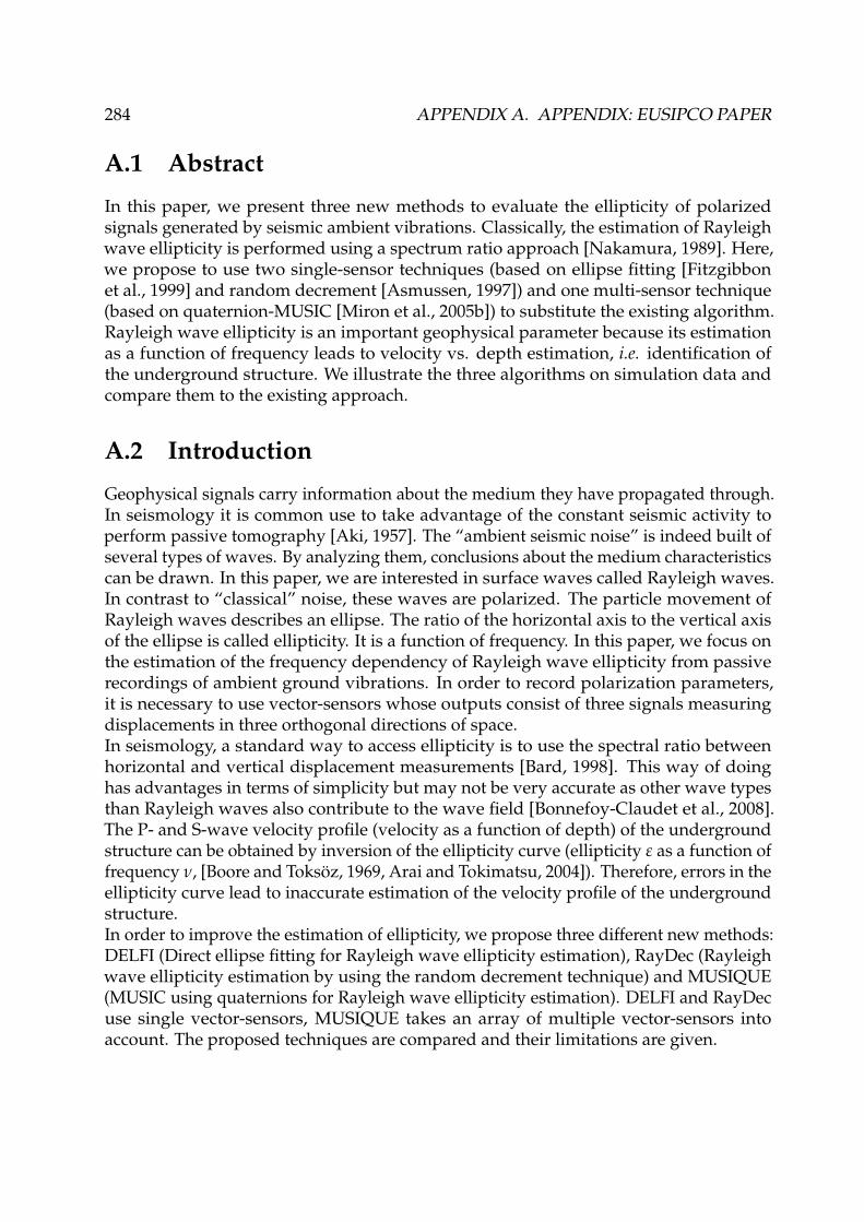
284 APPENDIX A. APPENDIX: EUSIPCO PAPER

A.1 Abstract

In this paper, we present three new methods to evaluate the ellipticity of polarizedsignals generated by seismic ambient vibrations. Classically, the estimation of Rayleighwave ellipticity is performed using a spectrum ratio approach [Nakamura, 1989]. Here,we propose to use two single-sensor techniques (based on ellipse fitting [Fitzgibbonet al., 1999] and random decrement [Asmussen, 1997]) and one multi-sensor technique(based on quaternion-MUSIC [Miron et al., 2005b]) to substitute the existing algorithm.Rayleigh wave ellipticity is an important geophysical parameter because its estimationas a function of frequency leads to velocity vs. depth estimation, i.e. identification ofthe underground structure. We illustrate the three algorithms on simulation data andcompare them to the existing approach.

A.2 Introduction

Geophysical signals carry information about the medium they have propagated through.In seismology it is common use to take advantage of the constant seismic activity toperform passive tomography [Aki, 1957]. The “ambient seismic noise” is indeed built ofseveral types of waves. By analyzing them, conclusions about the medium characteristicscan be drawn. In this paper, we are interested in surface waves called Rayleigh waves.In contrast to “classical” noise, these waves are polarized. The particle movement ofRayleigh waves describes an ellipse. The ratio of the horizontal axis to the vertical axisof the ellipse is called ellipticity. It is a function of frequency. In this paper, we focus onthe estimation of the frequency dependency of Rayleigh wave ellipticity from passiverecordings of ambient ground vibrations. In order to record polarization parameters,it is necessary to use vector-sensors whose outputs consist of three signals measuringdisplacements in three orthogonal directions of space.In seismology, a standard way to access ellipticity is to use the spectral ratio betweenhorizontal and vertical displacement measurements [Bard, 1998]. This way of doinghas advantages in terms of simplicity but may not be very accurate as other wave typesthan Rayleigh waves also contribute to the wave field [Bonnefoy-Claudet et al., 2008].The P- and S-wave velocity profile (velocity as a function of depth) of the undergroundstructure can be obtained by inversion of the ellipticity curve (ellipticity ε as a function offrequency ν, [Boore and Toksöz, 1969, Arai and Tokimatsu, 2004]). Therefore, errors in theellipticity curve lead to inaccurate estimation of the velocity profile of the undergroundstructure.In order to improve the estimation of ellipticity, we propose three different new methods:DELFI (Direct ellipse fitting for Rayleigh wave ellipticity estimation), RayDec (Rayleighwave ellipticity estimation by using the random decrement technique) and MUSIQUE(MUSIC using quaternions for Rayleigh wave ellipticity estimation). DELFI and RayDecuse single vector-sensors, MUSIQUE takes an array of multiple vector-sensors intoaccount. The proposed techniques are compared and their limitations are given.

A.3. RAYLEIGH WAVE ELLIPTICITY IN SEISMOLOGY 285

A.3 Rayleigh wave ellipticity in seismology

First, we introduce the term of Rayleigh wave ellipticity as understood in seismology.After briefly recalling the underlying physics, we present the signals we will use todetermine the ellipticity.

A.3.1 Surface waves and underground structureFour main wave types are important in seismology. P- and S-waves represent pressureand shear body waves, respectively. Rayleigh and Love waves are surface waves, i.e.they propagate along the earth’s surface. Their energy decreases as 1/r compared to 1/r2

for body waves where r is the distance to an earthquake hypocenter. Therefore surfacewaves are important for seismic hazard assessment.Love waves are transverse waves which are confined to the surface layer. Rayleighwaves, which are also called “ground roll”, are waves with a vertical and a horizontalcomponent. The movement of a particle under the influence of a Rayleigh wave describesan ellipse in the plane formed by the vertical axis and the wave propagation direction.At the surface of homogeneous halfspaces, the movement of the fundamental mode isretrograde, i.e. the horizontal movement advances the vertical movement by π/2 inphase. Prograde movement corresponds to a phase difference of −π/2.The underground structure of the earth’s surface is in general not homogeneous but con-sists of different sedimentary layers superposing the bedrock. Every layer has differentmechanical properties, e.g. P- and S-wave velocities. The properties of Rayleigh wavesare closely related to the underground structure. An important polarization parameterof Rayleigh waves is the ellipticity ε. It is a function of frequency ν. Figure A.1 shows arealistic model of the P- and S-wave velocity profile of an underground structure and thecorresponding ε(ν)-curve. Inversion techniques exist allowing the underground P- andS-wave velocity profiles to be derived from the ε(ν)-curve of the Rayleigh waves [Araiand Tokimatsu, 2004].The knowledge of the soil structure of a given site is important in order to estimate theground motion and the associated risk for buildings in the case of an earthquake.

A.3.2 Sensors and arrays

In seismology, the earth’s movements are recorded using vector-sensors called geophones.Such sensors are made of three co-located sensors recording the ground motion in threeorthogonal directions. As a result, the output signal is a 3D vector-valued time-series. Byconvention, the three sensors are aligned in north-south, east-west and vertical direction.A number of vector-sensors can be arranged to form an array. Thus, this configurationenables the measurement of the azimuth and velocity of incoming waves. In the follow-ing, the east-west signal of the vector-sensor will be denoted by x(t), the north-southsignal by y(t) and the vertical signal by z(t).

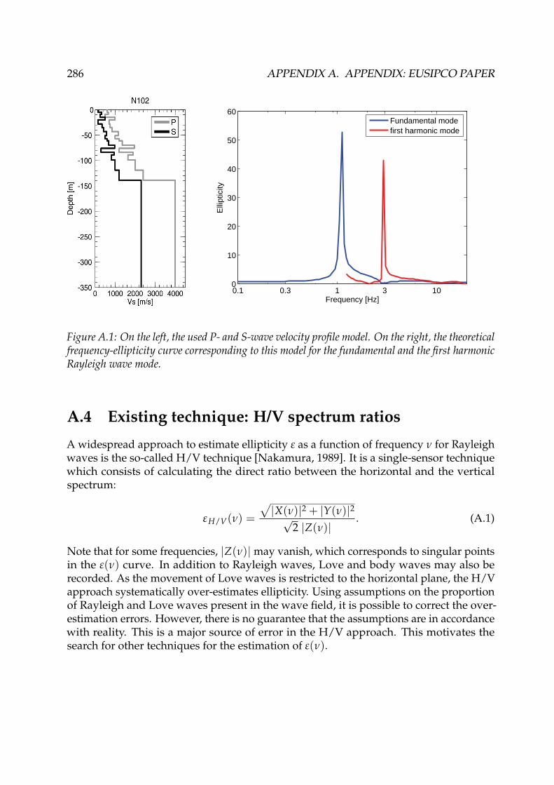
286 APPENDIX A. APPENDIX: EUSIPCO PAPER

0.1 0.3 1 3 100

10

20

30

40

50

60

Frequency [Hz]

Elli

ptic

ity

Fundamental modefirst harmonic mode

Figure A.1: On the left, the used P- and S-wave velocity profile model. On the right, the theoreticalfrequency-ellipticity curve corresponding to this model for the fundamental and the first harmonicRayleigh wave mode.

A.4 Existing technique: H/V spectrum ratios

A widespread approach to estimate ellipticity ε as a function of frequency ν for Rayleighwaves is the so-called H/V technique [Nakamura, 1989]. It is a single-sensor techniquewhich consists of calculating the direct ratio between the horizontal and the verticalspectrum:

εH/V(ν) =√|X(ν)|2 + |Y(ν)|2√

2 |Z(ν)|. (A.1)

Note that for some frequencies, |Z(ν)|may vanish, which corresponds to singular pointsin the ε(ν) curve. In addition to Rayleigh waves, Love and body waves may also berecorded. As the movement of Love waves is restricted to the horizontal plane, the H/Vapproach systematically over-estimates ellipticity. Using assumptions on the proportionof Rayleigh and Love waves present in the wave field, it is possible to correct the over-estimation errors. However, there is no guarantee that the assumptions are in accordancewith reality. This is a major source of error in the H/V approach. This motivates thesearch for other techniques for the estimation of ε(ν).

A.5. SINGLE-SENSOR APPROACH 287

A.5 Single-sensor approach

In this section, we present two approaches to perform ellipticity estimation using thesignal recorded on a single three-component vector-sensor. Their performances will beillustrated in Section A.7.

A.5.1 Direct ellipse fitting (DELFI)

Consider the vector-valued signal ~s(t) describing the movement of a soil particle in3D space with time, given as ~s(t) = [x(t) y(t) z(t)]T taking values in R3. First, ~s(t)is band-pass filtered around a frequency ν with bandwidth dν. Then, the followingprocessing is performed independently for each frequency.The filtered signal is cut in blocks of time length T = 1/ν. The total length of the signalis assumed to be much longer than T. Each time-window consists thus of N = T/dtsamples where dt is the sampling period. The three-component signal of one time-window is noted Sw = [Xw Yw Zw]T and is of dimension 3 × N. The polarizationof Rayleigh waves is confined to a vertical plane, in opposition to the movement ofnoise signals which lie in 3D space. In order to project the signal Sw onto a verticalplane, we use the covariance matrix Cw built by the two horizontal components byCw = [Xw Yw]T[Xw Yw].The Eigenvalue Decomposition (EVD) of Cw gives access to its eigenvalues λ1 andλ2 (ranked in increasing order, i.e. λ1 < λ2) and associated eigenvectors ~u1 and ~u2.The eigenvectors are normal vectors to two orthogonal vertical planes. The associatedeigenvalues are the sums of the squared distances between the data points and therespective planes.The 2D plane where the signal~sw(t) is mostly confined is the one orthogonal to ~u1 asit is associated to the smallest eigenvalue λ1, i.e. the corresponding plane is spannedby the eigenvector ~u2 and the vertical unit vector. The horizontal components of thetime-window signal Sw are then projected onto an axis to build a horizontal signal Hwby Hw = [Xw Yw] ·~u2. The 2D signal is then built by S′w = [Hw Zw]T.Finally, the ellipticity measurement is performed using a modified version of the ellipsefitting algorithm proposed by Fitzgibbon et al. [Fitzgibbon et al., 1999]. The modificationsof the algorithm ensure that the axes of the ellipse are in horizontal and vertical directions.The algorithm yields the horizontal axis hw, the vertical axis vw and a parameter d2

windicating the actual sum of squared distances between the data points and the fittedellipse.The ellipticity ε(ν) is calculated by averaging the found horizontal and vertical axes ofall signal blocks for the corresponding frequency using the distance parameter d2

w asweighting factor:

εDELFI(ν) = ∑ hw/d2w

∑ vw/d2w

. (A.2)

The only free parameter of the method is dν.

288 APPENDIX A. APPENDIX: EUSIPCO PAPER

A.5.2 Random decrement (RayDec)

The random decrement technique is commonly used to characterize dynamic parametersof buildings [Dunand, 2005, Michel et al., 2008]. It is classically applied to one-component(scalar valued) signals. We propose a three-component version of this technique in orderto estimate ε(ν).The following processing is performed independently for each frequency. First, the threecomponents of~s(t) are filtered in a frequency range of bandwidth dν around a centralfrequency ν. The filtered components are called xν(t), yν(t) and zν(t).The next step is to search for the times τi where the signal sign changes from negativeto positive on the vertical component (zν(τi) ≤ 0, zν(τi + dt) > 0). For each of these τi asignal block of length ∆ is stored on all three components. The number of buffered blocksthus depends on the analyzed signal itself. In order to compensate the natural π/2 phaseshift, i.e. 1/(4ν) in time, between the vertical and horizontal component signals of aRayleigh wave, a phase shift is applied to xν and yν. The buffered signals then are:

zν,b,i(t) = zν(τi + t),xν,b,i(t) = xν(τi − 1

4ν + t),yν,b,i(t) = yν(τi − 1

4ν + t).(A.3)

for 0 ≤ t ≤ ∆. Index i specifies the change of sign position while index b stands forbuffered. The east-west and north-south components, namely xν,b,i(t) and yν,b,i(t), ofevery buffered signal~sν,b,i(t) are then projected onto a single axis to build a horizontalcomponent in the following way:

hν,b,i(t) = sin ϑi · xν,b,i(t) + cos ϑi · yν,b,i(t). (A.4)

The azimuth angle ϑi is chosen to maximize the correlation C(ϑi) =∫ ∆

0 zν,b,i(t) · hν,b,i(t)dtbetween the vertical signal zν,b,i(t) and the horizontal signal hν,b,i(t). The azimuth angleϑi is thus obtained by

ϑi = tan−1

(∫ ∆0 zν,b,i(t) · xν,b,i(t)dt∫ ∆0 zν,b,i(t) · yν,b,i(t)dt

). (A.5)

From the two possible ϑi ∈ [0◦, 360◦[ satisfying equation (A.5) we choose the one leadingto a positive correlation. At this point, the method does not distinguish between progradeand retrograde particle motion as prograde Rayleigh waves are treated as retrogradewaves arriving from the opposite azimuth.Although the angle ϑi maximizes the correlation, zν,b,i(t) and hν,b,i(t) can still be weaklycorrelated. Therefore, a correlation factor defined by

cν,b,i =

∫ ∆0 zν,b,i(t) · hν,b,i(t)dt√∫ ∆

0 z2ν,b,i(t)dt ·

∫ ∆0 h2

ν,b,i(t)dt(A.6)

A.6. MULTIPLE-SENSOR APPROACH (MUSIQUE) 289

is used as weighting factor in the summation of the signals zν,b,i(t) and hν,b,i(t) :

zν,s(t) = ∑i

c2ν,b,i · zν,b,i(t) (A.7)

hν,s(t) = ∑i

c2ν,b,i · hν,b,i(t). (A.8)

Finally, the ellipticity is obtained by

εRayDec(ν) =

√√√√∫ ∆0 h2

ν,s(t)dt∫ ∆0 z2

ν,s(t)dt. (A.9)

Repeated execution of this algorithm over the whole frequency range yields the frequency-ellipticity curve. The length of the buffered signal ∆ and the width of the frequency filterdν can be chosen arbitrarily.

A.6 Multiple-sensor approach (MUSIQUE)

In this section, we propose a way to take advantage of array measurements. The proposedapproach is based on MUSIC algorithm and uses two of its versions: “classical” MUSICto perform wave identification and “quaternion” MUSIC for ellipticity estimation. Thearray consists of NS three-component sensors. The NS time sample records are cutinto blocks of NT = nP/(ν dt) data points each, where nP is the number of periodscorresponding to the frequency ν in the block and dt the sampling period. The cut timesamples are stored in three NS × NT data matrices Si(t) with i = 1 for vertical, i = 2 foreast−west and i = 3 for north− south component. Fourier transform of these three datamatrices yields the three matrices Si(ν) of dimensions NS × NT.

A.6.1 First step: Azimuth estimationThe first step of our approach is to perform a “classical” MUSIC to identify the azimuthand velocity of an incoming wave. Note that this is a narrow-band MUSIC of bandwidthdν. Therefore, the spectral matrix is computed. Each one-component spectral matrixMi(ν) ∈ CNS×NS is given by Mi(ν) = Si(ν)S†

i (ν). Then, the total sample covariancematrix M(ν) ∈ CNS×NS is obtained by M(ν) = ∑3

i=1 Mi(ν).The Nbig biggest eigenvalues of the matrix M(ν) are identified to belong to the signalsubspace and the other (NS − Nbig) to the noise subspace. It should be noted that due tothe later performed projection into a plane the technique can only yield reliable results ifthe wave field is dominated by one wave and therefore Nbig = 1. The noise subspaceG(ν) ∈ CNS×(NS−Nbig) is hence built using the associated eigenvectors.An incident Rayleigh wave with azimuth ϑ and phase velocity c is assumed. Theassociated wave vector is thus ~κ(ϑ) = [− sin ϑ − cos ϑ 0]T and the time-delay vector~δ(ν, ϑ, c) ∈ RNS×1 is given by

~δ(ν, ϑ, c) =2πν

cR~κ(ϑ), (A.10)

290 APPENDIX A. APPENDIX: EUSIPCO PAPER

where R ∈ RNS×3 is the matrix of the positions of the array sensors and c the wavevelocity. This leads to the steering vector ~fl(ν, ϑ, c) = exp (−i~δ(ν, ϑ, c))/

√NS. The

MUSIC functional F(ν, ϑ, c) is finally given by:

F(ν,ϑ,c) =1

~γ†(ν,ϑ,c)G(ν)G†(ν)~γ(ν,ϑ,c). (A.11)

A grid search is performed in order to find the set of parameters (ϑ0, c0) maximizing thisfunctional.Now, as the movement of Rayleigh waves is confined to a plane spanned by the wavevector and the vertical axis, the original signals are projected into the vertical planespanned by the wave vector just found. This means that the original vertical signal isleft unchanged and the two horizontal signals are rotated using ϑ0. The new signal Sp(t)consists of two matrices, Sp1(t) and Sp2(t), as it is confined to a 2D plane (instead of 3components). It is obtained from the original signal by:

Sp1(t) = S1(t) (A.12)

Sp2(t) = − sin ϑ0 · S2(t)− cos ϑ0 · S3(t). (A.13)

Fourier transforms of Sp1(t) and Sp2(t) give the matrices Sp1(ν) and Sp2(ν). Now thatthe signals are confined in the propagation plane of the Rayleigh wave, we can proceedto the estimation of ellipticity.

A.6.2 Second step: Ellipticity estimation

The second step of our approach consists in using a quaternion MUSIC algorithmto estimate the polarization parameters of the identified wave. Miron et al. [2006]demonstrated its ability to perform polarization estimation. Therefore, we first build aquaternion valued data matrix Sq(ν) ∈HNS×NT in the frequency domain [Miron et al.,2006]:

Sq(ν) = <(Sp1(ν)) + i · <(Sp2(ν)) + j · =(Sp1(ν)) + k · =(Sp2(ν)), (A.14)

where i, j and k are the three quaternion imaginary units [Ward, 1997]. The quaternionvalued spectral matrix Mq(ν) is given by Mq(ν) = Sq(ν) S†

q(ν). Here again, the noisesubspace Gq(ν) is built by the (NS − Nbig) eigenvectors corresponding to the smallesteigenvalues, where Nbig is the same number of sources as defined in the first step. Inagreement with Miron et al. [2006], the quaternion steering vector is given by:

~γq(ν,ρ,ϕ) = [cos(ρ) + i sin(ρ)ejϕ]e−j~δ(ν,ϑ0,c0)/√

NS (A.15)

where ρ and ϕ are the polarization parameters of the wave and ~δ(ν, ϑ0, c0) is the arraydelay vector given by equation (A.10) with ϑ = ϑ0 and c = c0. The ellipticity ε is the ratioof the amplitudes of horizontal and vertical motion, i.e.

εMUSIQUE = sin ρ/ cos ρ = tan ρ. (A.16)

A.7. SIMULATION 291

ϕ is the phase difference between the horizontal and the vertical signal. Note that weomitted the ν dependency of ρ and ϕ in eq. (A.15), but it should not be forgotten that theirvalues depend on ν. A grid search yields the set of parameters (ρ0, ϕ0) that maximizesthe quaternion MUSIC functional

Fq(ν,ρ,ϕ) =1

~γ†q(ν,ρ,ϕ)Gq(ν)G†

q(ν)~γq(ν,ρ,ϕ))(A.17)

Instead of using the parameter ρ to describe the ellipticity ε of the wave, it is possible touse ellipticity itself. However, as ellipticity values are in principle not limited, one wouldhave to perform the parameter search for 0 ≤ ε ≤ ∞. Therefore, it is advantageous tolimit the search to 0 ≤ ρ ≤ π/2 and to define ellipticity by equation (A.16). The phasedifference ϕ is searched in the intervall [0, 2π[. For a retrograde Rayleigh wave, the phasedifference will be found around π/2, for a prograde Rayleigh wave it will be about 3π/2.The preceding processing is performed for every signal block of length NT. For eachfrequency ν, the ellipticities of the signal blocks are averaged using the reciprocal valueof the difference of ϕ from the the theoretical phase difference (π/2 for retrograde, 3π/2for prograde) and the signal energy of the signal block as weighting factors. In this way,the ellipticity curve ε(ν) is estimated.The performances of the proposed multiple-sensor method are presented in the nextsection.

A.7 Simulation

In order to show the performances of the three proposed algorithms, we applied themto a set of synthetic seismic ambient vibrations. Model N102 of an international blindtest benchmark [Cornou et al., 2009] was used as underground structure. The P- andS-wave velocity profiles of the model, as well as the associated theoretical frequency-ellipticity curve, are shown in figure A.1. 620 seconds of synthetic ambient vibrationswere simulated as follows. Signal sources were modeled by forces with random orien-tation and amplitude located 0.5 m below the surface [Moczo and Kristek, 2002]. Theforces were distributed randomly in time and space. The time function of each sourcewas a delta-like signal with a flat Fourier frequency-amplitude spectrum between 0.1and 20 Hz. The associated wave field was computed by using the wavenumber-basedtechnique of Hisada [Hisada, 1994, 1995] and contains all body and surface wave types.As the goal of this investigation is the Rayleigh wave ellipticity as a function of frequency,Love and body waves can be considered as “noise”. However, the signal-to-noise ratiois unknown and the robustness of the methods under different signal-to-noise ratioscannot be investigated. As the signal generation mimics the generation of real seismicambient vibrations this case can though be considered realistic.The recordings were simulated for sixty seismic sensors. Their spatial distribution isshown in figure A.2. The noise sources distribution covered all possible azimuths anddistances up to around 1200 m from the origin. Therefore, every seismic sensor representsa different set of data. As the underground structure is the same at every point of themodel, the theoretical ellipticity is the same for each sensor.

292 APPENDIX A. APPENDIX: EUSIPCO PAPER

−500 −250 0 250 500

−400

−200

0

200

Distance [m]

Dis

tanc

e [m

]

Figure A.2: Layout of the sixty sensors forming ten seven-sensor arrays. Some stations belong toseveral arrays.

For H/V, DELFI and RayDec, the sixty sensors were used independently. To testMUSIQUE, ten arrays of seven sensors each were formed, some sensors belongingto several arrays. The Rayleigh wave ellipticity estimations of the three presented newmethods and the classical H/V technique are shown in figure A.3 in comparison to thetheoretical ellipticity curve of the model.The used free parameters are: for DELFI, dν = 0.2ν; for RayDec, dν = 0.2ν and ∆ = 10/ν;for MUSIQUE, dν = 0.2ν and nP = 10.The H/V technique overestimates ellipticity considerably, especially at frequencies aboveand below the peak frequency. Compared to H/V, DELFI only improves the peakfrequency estimation. As it works on the raw signals, it does not eliminate Love andbody waves and therefore its results are close to H/V results. The RayDec curve is veryclose to the theoretical curve over the whole analyzed frequency range. RayDec is astatistical method which averages over a large number of time-windows to efficientlyeliminate other wave types than Rayleigh waves. That is why its results are very closeto the theoretical curve. For MUSIQUE, the results are in good agreement with theoryover the whole frequency range, but compared to RayDec, the error bars are larger.However, MUSIQUE does not suppress Love and body waves but also shows goodresults in identifying ellipticity. As the curve is the average for ten arrays, its resultscould propably be better with more arrays or more signal analysed. Optimisation of thearray layouts (array aperture and geometry) could also improve the results.

A.7. SIMULATION 293

0.5 1 2 50

5

10

15

20

Elli

ptic

ity

Frequency [Hz]

MODELH/V

0.5 1 2 50

5

10

15

20

Elli

ptic

ity

Frequency [Hz]

MODELDELFI

0.5 1 2 50

5

10

15

20

Elli

ptic

ity

Frequency [Hz]

MODELRAYDEC

0.5 1 2 50

5

10

15

20

Elli

ptic

ity

Frequency [Hz]

MODELMUSIQUE

Figure A.3: Rayleigh wave ellipticity curves obtained by analyzing 620 seconds of syntheticseismic ambient vibrations by H/V, DELFI, RayDec and MUSIQUE techniques in comparison tothe theoretical ellipticity curve of the model. For H/V, DELFI and RayDec, the average curvesof 60 sensors are shown with the corresponding error range. For MUSIQUE, the average curvewith error margin for ten arrays is shown.

In testing the methods, we have stated that RayDec requires a minimum signal length ofsome minutes to give stable results. DELFI and MUSIQUE, in contrast, do not requirea minimum signal length and are thus applicable to non-stationary wave trains asproduced in earthquakes. As MUSIQUE uses array measurements, it also gives anestimate of the azimuth and wave velocity. Therefore, it is also possible to distinguishbetween prograde and retrograde Rayleigh wave movement. DELFI and RayDec donot give the wave velocity and give two possible azimuths. Therefore, they cannotdistinguish between prograde and retrograde Rayleigh waves.

294 APPENDIX A. APPENDIX: EUSIPCO PAPER

A.8 Conclusion

The three new methods have been succesfully applied to synthetic noise data and haveproven their ability to estimate the frequency-ellipticity curves of Rayleigh waves. Thefurther work is to quantify the differences between the results of the method and thetheory and to test the methods on other simulation data. Completing those tasks wouldvalidate the applicability of the proposed methods to real seismic data.

Acknowledgments

Noise synthetics were performed at the Service Commun de Calcul Intensif (SCCI) ofGrenoble observatory, France (OSUG). This work is supported by the NERIES Europeanproject and the ANR QSHA project.

Bibliography

K. Aki. Space and time spectra of stationary stochastic waves, with special reference tomicrotremors. Bull. Earthquake Res. Inst. Tokyo Univ., 35:415–456, 1957.

K. Aki and P. G. Richards. Quantitative Seismology. University Science Books, 2 edition,2002.

H. Arai and K. Tokimatsu. S-wave velocity profiling by inversion of microtremor H/Vspectrum. Bull. Seismol. Soc. Am., 94:53–63, 2004.

H. Arai and K. Tokimatsu. S-wave velocity profiling by joint inversion of microtremordispersion curve and horizontal-to-vertical (H/V) spectrum. Bull. Seismol. Soc. Am., 95:1766–1778, 2005. doi: 10.1785/0120040243.

H. Arai and K. Tokimatsu. Evaluation of local site effects based on microtremor H/Vspectra. In The Effects of Surface Geology on Seismic Motion. Balkema, Rotterdam, 1998.

J. C. Asmussen. Modal analysis based on the random decrement technique. PhD thesis,University of Aalborg, 1997.

M. W. Asten and J. D. Henstridge. Array estimators and the use of microseisms forreconnaissance of sedimentary basins. Geophysics, 49:1828–1837, 1984. doi: 10.1190/1.1441596.

P.-Y. Bard. Microtremor measurements: a tool for site effect estimation? In SecondInternational Symposium on the Effects of Surface Geology on seismic motion, Yokohama,December 1-3, 1998, volume 3, pages 1251–1279. Balkema, 1998.

T. Bardainne, P. Gaillot, N. Dubos-Sallée, J. Blanco, and G. Sénéchal. Characterization ofseismic waveforms and classification of seismic events using chirplet atomic decompo-sition. Example from the Lacq gas field (Western Pyrenees, France). Geophys. J. Int.,166:699–718, 2006. doi: 10.1111/j.1365-246X.2006.03023.x.

C. Beauval, P.-Y. Bard, P. Moczo, and J. Kristek. Quantification of frequency-dependentlenghtening of seismic ground-motion duration due to local geology: Applications tothe Volvi area (Greece). Bull. Seismol. Soc. Am., 93:371–385, 2003.

B. Bettig, P.-Y. Bard, F. Scherbaum, J. Riepl, F. Cotton, C. Cornou, and D. Hatzfeld. Anal-ysis of dense array noise measurements using the modified spatial auto-correlationmethod (SPAC): application to the Grenoble area. Boll. Geof. Teor. Appl., 42:281–304,2001.

295

296 BIBLIOGRAPHY

S. Bonnefoy-Claudet. Nature du bruit de fond sismique : implications pour les études des effetsde site. PhD thesis, Université Joseph Fourier Grenoble, 2004.

S. Bonnefoy-Claudet, C. Cornou, P.-Y. Bard, F. Cotton, P. Moczo, J. Kristek, and D. Fäh.H/V ratio: a tool for site effects evaluation. Results from 1-D noise simulations. Geophys.J. Int., 167:827–837, 2006. doi: 10.1111/j.1365-246X.2006.03154.x.

S. Bonnefoy-Claudet, A. Köhler, C. Cornou, M. Wathelet, and P.-Y. Bard. Effects ofLove waves on microtremor H/V ratio. Bull. Seismol. Soc. Am., 98:288–300, 2008. doi:10.1785/0120070063.

D. M. Boore and M. N. Toksöz. Rayleigh wave particle motion and crustal structure. Bull.Seismol. Soc. Am., 59:331–346, 1969.

M. Born and E. Wolf. Principles of Optics. Cambridge University Press, 7th edition, 1999.

J. L. Brenner. Matrices of quaternions. Pacific J. Math., 1:329–335, 1951.

T. M. Brocher. Compressional and shear wave velocity versus depth in the San FranciscoBay Area, California: Rules for USGS Bay Area velocity model 05.0.0. U.S. GeologicalSurvey Open-File Report 2005-1317 Version 1.0, 2005.

T. M. Brocher. Compressional and shear-wave velocity versus depth relations for commonrock types in Northern California. Bull. Seismol. Soc. Am., 98:950–968, 2008. doi:10.1785/0120060403.

T. M. Brocher, E. E. Brabb, R. D. Catchings, G. S. Fuis, T. E. Fumal, R. C. Jachens, A. S.Jayko, R. E. Kayen, R. J. McLaughlin, T. Parsons, M. J. Rymer, R. G. Stanley, and C. M.Wentworth. A crustal-scale 3-D seismic velocity model for the San Francisco Bay area,California. Eos Trans. AGU, 78:F435, 1997.

I. N. Bronstein, K. A. Semendjajew, G. Musiol, and H. Mühlig. Taschenbuch der Mathematik.Verlag Harri Deutsch, 2001.

C. Brosseau. Fundamentals of Polarized Light: A Statistical Optics Approach. Wiley-Interscience, 1998.

J. Capon. High-resolution frequency-wavenumber spectrum analysis. Proc. IEEE, 57:1408–1418, 1969.

I. Cho, T. Tada, and Y. Shinozaki. Assessing the applicability of the spatial autocorrelationmethod: A theoretical approach. J. Geophys. Res., 113:B06307, 2008. doi: 10.1029/2007JB005245.

J. J. Christensen and J. Hald. Beamforming. Technical report, Brüel & Kjær, 2004.

C. Cornou. Traitement d’antenne et imagerie sismique dans l’agglomération grenobloise (Alpesfrançaises) : implications pour les effets de site. PhD thesis, Université Joseph FourierGrenoble, 2002.

BIBLIOGRAPHY 297

C. Cornou, P.-Y. Bard, and M. Dietrich. Contribution of dense array analysis to theidentification and quantification of basin-edge induced waves, part I: Methodology.Bull. Seismol. Soc. Am., 93:2604–2623, 2003a.

C. Cornou, P.-Y. Bard, and M. Dietrich. Contribution of dense array analysis to theidentification and quantification of basin-edge induced waves, part II: Application toGrenoble basin (French Alps). Bull. Seismol. Soc. Am., 93:2624–2648, 2003b.

C. Cornou, M. Ohrnberger, D. M. Boore, K. Kudo, and P.-Y. Bard. Derivation of structuralmodels from ambient vibration array recordings: Results from an international blindtest. In Proc. 3rd Int. Symp. on the Effects of Surface Geology on Seismic Motion, Grenoble,30 August - 01 September, 2006, volume 2, pages 1127–1217. LCPC Editions, 2009.

K. De Meersman, M. van der Baan, and J.-M. Kendall. Signal extraction and automatedpolarization analysis of multicomponent array data. Bull. Seismol. Soc. Am., 96:2415–2430, 2006.

G. Di Giulio, C. Cornou, M. Ohrnberger, M. Wathelet, and A. Rovelli. Deriving wavefieldcharacteristics and shear-velocity profiles from two-dimensional small-aperture arraysanalysis of ambient vibrations in a small-size alluvial basin, Colfiorito, Italy. Bull.Seismol. Soc. Am., 96:1915–1933, 2006. doi: 10.1785/0120060119.

G. Di Giulio, A. Savvaidis, N. Theodulidis, M. Ohrnberger, B. Endrun, M. Wathelet,C. Cornou, F. Renalier, and P.Y. Bard. Inversion of surface wave dispersion at Europeanstrong motion sites using a multi-model parameterization and an information-theoreticapproach. In Proc. 14th European Conference on Earthquake Engineering, 30 August - 03September 2010, Ohrid, Republic of Macedonia, 2010.

D. Dolenc and D. Dreger. Microseisms observations in the Santa Clara Valley, California.Bull. Seismol. Soc. Am., 95:1137–1149, 2005. doi: 10.1785/0120040060.

D. Dolenc, D. Dreger, and S. Larsen. Basin structure influences on the propagation ofteleseismic waves in the Santa Clara Valley, California. Bull. Seismol. Soc. Am., 95:1120–1136, 2005. doi: 10.1785/0120040059.

F. Dunand. Pertinence du bruit de fond sismique pour la caractérisation dynamique et l’aide audiagnostic sismique des structures de génie civil. PhD thesis, Université Joseph FourierGrenoble, 2005.

B. Endrun. Love wave contribution to the ambient vibration H/V amplitude peakobserved with array measurements. J. Seismol., 2010. doi: 10.1007/s10950-010-9191-x.

B. Endrun and F. Renalier. Report on in-situ measurements at the 20 selected sites.NERIES deliverable JRA4 D2, available at http://www.neries-eu.org, 2008.

B. Endrun, M. Ohrnberger, and A. Savvaidis. On the repeatability and consistency ofthree-component ambient vibration array measurements. Bull. Earthquake Eng., 8:535–570, 2010. doi: 10.1007/s10518-009-9159-9.

298 BIBLIOGRAPHY

D. Fäh, F. Kind, and D. Giardini. A theoretical investigation of average H/V ratios.Geophys. J. Int., 145:535–549, 2001.

D. Fäh, F. Kind, and D. Giardini. Inversion of local S-wave velocity structures fromaverage H/V ratios, and their use for the estimation of site-effects. Journal of Seismology,7:449–467, 2003.

D. Fäh, G. Stamm, and H.-B. Havenith. Analysis of three-component ambient vibrationarray measurements. Geophys. J. Int., 172:199–213, 2008. doi: 10.1111/j.1365-246X.2007.03625.x.

D. Fäh, M. Wathelet, M. Kristekova, H. Havenith, B. Endrun, G. Stamm, V. Poggi,J. Burjanek, and C. Cornou. Using ellipticity information for site characterisation.NERIES deliverable JRA4 D4, available at http://www.neries-eu.org, 2009.

E. H. Field. Spectral amplification in a sediment-filled valley exhibiting clear basin-edge-induced waves. Bull. Seismol. Soc. Am., 86:991–1005, 1996.

A. W. Fitzgibbon, M. Pilu, and R. B. Fisher. Direct least-squares fitting of ellipses. IEEETrans. Pattern Analysis and Machine Intelligence, 21:476–480, 1999.

J. B. Fletcher, J. Boatwright, and A. G. Lindh. Wave propagation and site response in theSanta Clara Valley. Bull. Seismol. Soc. Am., 93:480–500, 2003.

E. A. Flinn. Signal analysis using rectilinearity and direction of particle motion. Proc.IEEE, 53:1874–1876, 1965.

A. Frankel, D. Carver, E. Cranswick, T. Bice, R. Sell, and S. Hanson. Observations ofbasin ground motions from a dense seismic array in San Jose, California. Bull. Seismol.Soc. Am., 91:1–12, 2001.

S. Gaffet, C. Larroque, A. Deschamps, and F. Tressols. A dense array experiment for theobservation of waveform perturbations. Soil Dynamics and Earthquake Engineering, 17:475–484, 1998.

A. V. Gorbatikov, M. Yu. Stepanova, and G. E. Korablev. Microseismic field affected bylocal geological heterogeneities and microseismic sounding of the medium. Izvestiya,Physics of the Solid Earth, 44:577–592, 2007. doi: 10.1134/S1069351308070082.

P. Gouédard, C. Cornou, and P. Roux. Phase-velocity dispersion curves and small-scalegeophysics using noise correlation slantstack technique. Geophys. J. Int., 172:971–981,2008. doi: 10.1111/j.1365-246X.2007.03654.x.

A. Grandi, A. Mazzotti, and E. Stucchi. Multicomponent velocity analysis with quater-nions. Geophysical Prospecting, 55:761–777, 2007. doi: 10.1111/j.1365-2478.2007.00657.x.

P. Guéguen, J.-L. Chatelain, B. Guillier, H. Yepes, and J. Egred. Site effect and damagedistribution in Pujili (Ecuador) after the 28 March 1996 earthquake. Soil Dynamics andEarthquake Engineering, 17:329–334, 1998.

BIBLIOGRAPHY 299

E. Haghshenas, P.-Y. Bard, N. Theodulidis, and SESAME WP04 team. Empirical evalu-ation of microtremor H/V spectral ratio. Bulletin of Earthquake Engineering, 6:75–108,2008.

W. R. Hamilton. On quaternions, or on a new system of imagineries in algebra. TheLondon, Edinburgh and Dublin Philosophical Magazine and Journal of Science, 1844-50.

W. R. Hamilton. On the geometrical interpretation of some results obtained by calculationwith biquaternions. Proc. of the Royal Irish Academy, 5:388–390, 1853.

D. G. Harkrider. Surface waves in multilayered elastic media, I. Rayleigh and Lovewaves from buried sources in a multilayered elastic half-space. Bull. Seismol. Soc. Am.,54:627–679, 1964.

D. G. Harkrider and D. L. Anderson. Computation of surface wave dispersion formultilayered anisotropic media. Bull. Seismol. Soc. Am., 52:321–332, 1962.

S. Hartzell, D. Carver, R. A. Williams, S. Harmsen, and A. Zerva. Site response, shallowshear-wave velocity, and wave propagation at the san jose, california, dense seismicarray. Bull. Seismol. Soc. Am., 93:443–464, 2003. doi: 10.1785/0120020080.

S. Hartzell, S. Harmsen, R. A. Williams, D. Carver, A. Frankel, G. Choy, P.-C. Liu, R. C.Jachens, T. M. Brocher, and C. M. Wentworth. Modeling and validation of a 3D velocitystructure for the Santa Clara Valley, California, for seismic-wave simulations. Bull.Seismol. Soc. Am., 96:1851–1881, 2006. doi: 10.1785/0120050243.

S. Hartzell, L. Ramirez-Guzman, D. Carver, and P. Liu. Short baseline variations in siteresponse and wave-propagation effects and their structural causes: Four examples inand around the Santa Clara Valley, California. Bull. Seismol. Soc. Am., 100:2264–2286,2010. doi: 10.1785/0120090278.

Y. Hisada. An efficient method for computing Green’s functions for a layered halfspacewith sources and receivers at close depths. Bull. Seismol. Soc. Am., 84:1456–1472, 1994.

Y. Hisada. An efficient method for computing Green’s functions for a layered halfspacewith sources and receivers at close depths (part 2). Bull. Seismol. Soc. Am., 85:1080–1093,1995.

M. Hobiger, P.-Y. Bard, C. Cornou, and N. Le Bihan. Single station determination ofRayleigh wave ellipticity by using the random decrement technique (RayDec). Geophys.Res. Lett., 36:L14303, 2009a. doi: 10.1029/2009GL038863.

M. Hobiger, N. Le Bihan, C. Cornou, and P.-Y. Bard. Rayleigh wave ellipticity estimationfrom ambient seismic noise using single and multiple vector-sensor techniques. In17th European Signal Processing Conference, Glasgow, UK, 24-28 August, 2009, 2009b.

M. Hobiger, C. Cornou, P.-Y. Bard, N. Le Bihan, and M. Wathelet. Inversion of Rayleighwave ellipticity measurements, Part I: Theoretical aspects. submitted to Geophys. J.Int., 2010a.

300 BIBLIOGRAPHY

M. Hobiger, C. Cornou, G. Di Giulio, B. Endrun, F. Renalier, A. Savvaidis, P.-Y. Bard,S. Hailemikael, N. Le Bihan, M. Ohrnberger, N. Theodulidis, and M. Wathelet. In-version of Rayleigh wave ellipticity measurements, Part II: Application to real datameasurements. submitted to Geophys. J. Int., 2010b.

C. I. Huerta, J. M. Roesset, and K. H. Stokoe. Evaluation of the random decrementmethod for in-situ soil properties. In The Effects of Surface Geology on Seismic Motion,pages 749–756. Balkema, Rotterdam, 1998.

A. Jurkevics. Polarization analysis of three-component array data. Bull. Seismol. Soc. Am.,78:1725–1743, 1988.

I. L. Kantor and A. S. Solodovnikov. Hypercomplex Numbers. Springer-Verlag, 1989.

H. Kawase. The cause of the damage belt in Kobe: "the basin-edge effect", constructiveinterference of the direct S-wave with the basin-induced diffracted/Rayleigh waves.Seism. Res. Lett., 67:25–34, 1996.

H. Kawase and K. Aki. A study on the response of a soft basin for incident S, P, andRayleigh waves with special reference to the long duration observed in Mexico City.Bull. Seismol. Soc. Am., 79:1361–1382, 1989.

A. Köhler, M. Ohrnberger, and F. Scherbaum. The relative fraction of Rayleigh andLove waves in ambient vibration wavefields at different European sites. In Proc. 3rdInt. Symp. on the Effects of Surface Geology on Seismic Motion, Grenoble, 30 August - 01September, 2006, volume 1, pages 351–360, 2006.

A. Köhler, M. Ohrnberger, F. Scherbaum, M. Wathelet, and C. Cornou. Assessing thereliability of the modified three-component spatial autocorrelation technique. Geophys.J. Int., 168:779–796, 2007. doi: 10.1111/j.1365-246X.2006.03253.x.

K. Konno and T. Ohmachi. Ground-motion characteristics estimated from spectral ratiobetween horizontal and vertical components of microtremor. Bull. Seismol. Soc. Am.,88:228–241, 1998.

R. T. Lacoss, E. J. Kelly, and M. N. Toksöz. Estimation of seismic noise structure usingarrays. Geophysics, 34:21–38, 1969.

J.-L. Lacoume, P.-O. Amblard, and P. Comon. Statistiques d’ordre supérieur pour le traitementdu signal. Masson, 1997.

T. Lay and T. C. Wallace. Modern Global Seismology. Academic Press, 1995.

N. Le Bihan and J. Mars. Singular value decomposition of quaternion matrices: A newtool for vector-sensor signal processing. Signal Processing, 84:1177–1199, 2004.

B. LeBrun, D. Hatzfeld, and P.-Y. Bard. Site effect study in urban area: Experimentalresults in Grenoble (France). Pure appl. geophys., 158:2543–2557, 2001.

BIBLIOGRAPHY 301

H. C. Lee. Eigenvalue and canonical forms of matrices with quaternion coefficients. Proc.of the Royal Irish Academy, 52:253–261, 1949.

J. Lermo and F. J. Chávez-García. Are microtremors useful in site response evaluation?Bull. Seismol. Soc. Am., 84:1350–1364, 1994.

P. G. Malischewsky and F. Scherbaum. Love’s formula and H/V-ratio (ellipticity) ofrayleigh waves. Wave motion, 40:57–67, 2004.

S. Marcos, editor. Les méthodes à haute résolution - traitement d’antenne et analyse spectrale.Editions HERMES, 1998.

J. Max and J.-L. Lacoume. Méthodes et techniques de traitement du signal et applications auxmesures physiques - 1. Principes généraux et méthodes classiques. Masson, 5 edition, 1996.

C. Michel, P. Guéguen, and P.-Y. Bard. Dynamic parameters of structures extracted fromambient vibration measurements: An aid for the seismic vulnerability assessment ofexisting buildings in moderate seismic hazard regions. Soil Dynamics and EarthquakeEngineering, 28:593–604, 2008.

S. Miron. Méthodes multilinéaires et hypercomplexes en traitement d’antenne multicomposantehaute résolution. PhD thesis, INP Grenoble, 2005.

S. Miron, N. Le Bihan, and J. Mars. Vector-sensor MUSIC for polarized seismic sourceslocalization. EURASIP J. Appl. Signal Process., pages 74–84, 2005a.

S. Miron, N. Le Bihan, and J. I. Mars. High resolution vector-sensor array processingusing quaternions. In IEEE International Conference on Statistical Signal Processing,Bordeaux, France, 2005, 2005b.

S. Miron, N. Le Bihan, and J. Mars. Quaternion-MUSIC for vector-sensor array processing.IEEE Trans. Signal Process., 54:1218–1229, 2006.

P. Moczo and J. Kristek. FD code to generate noise synthetics. Sesame report D02.09,available at http://SESAME-FP5.obs.ujf-grenoble.fr, 2002.

J. F. Montalbetti and E. R. Kanasewich. Enhancement of teleseismic body phases with apolarization filter. Geophys. J. R. astr. Soc., 21:119–129, 1970.

M. L. Moran and D. G. Albert. Source location and tracking capability of a small seismicarray. Technical report, CRREL, 1996.

H. Morikawa, S. Sawada, and J. Akamatsu. A method to estimate phase velocities ofRayleigh waves using microseisms simultaneously observed at two sites. Bull. Seismol.Soc. Am., 94:961–976, 2004.

Y. Nakamura. A method for dynamic characteristics estimation of subsurface usingmicrotremor on the ground surface. Quarterly reports of the Railway Technical ResearchInstitute Tokyo, 30:25–33, 1989.

302 BIBLIOGRAPHY

M. Nogoshi and T. Igarashi. On the amplitude characteristics of microtremor (part 2). J.Seism. Soc. Japan, 24:26–40, 1971. in Japanese with English abstract.

H. Okada. Theory of efficient array observations of microtremors with special referenceto the SPAC method. Exploration Geophysics, 37:73–85, 2006.

C. B. Park, R. D. Miller, and J. Xia. Multichannel analysis of surface waves. Geophysics,64:800–808, 1999.

S. Parolai, M. Picozzi, S. M. Richwalski, and C. Milkereit. Joint inversion of phasevelocity dispersion and H/V ratio curves from seismic noise recordings using a geneticalgorithm, considering higher modes. Geophys. Res. Lett., 32:L01303, 2005. doi: 10.1029/2004GL021115.

G. A. Phelps, R. W. Graymer, R. C. Jachens, D. A. Ponce, R. W. Simpson, and C. M.Wentworth. Three-dimensional geologic map of the Hayward Fault zone, San FranciscoBay region, California. U.S. Geological Survey Scientific Investigations Map 3045,http://pubs.usgs.gov/sim/3045/, 2008.

W. S. Phillips and K. Aki. Site amplification of coda waves from local earthquakes incentral California. Bull. Seismol. Soc. Am., 76:627–648, 1986.

M. Picozzi, S. Parolai, and S. M. Richwalski. Joint inversion of H/V ratios and dispersioncurves from seismic noise: Estimating the S-wave velocity of bedrock. Geophys. Res.Lett., 32:L11308, 2005. doi: 10.1029/2005FL022878.

M. Picozzi, F. Sabetta, N. Theodulidis, S. Zacharopoulos, A. Savvaidis, P.-Y. Bard,C. Cornou, P. Guéguen, D. Fäh, I. Kalogeras, S. Akkar, D. Rinaldis, and G. Tanir-can. Selected sites and available information. NERIES deliverable JRA4 D1, availableat http://www.neries-eu.org, 2007.

A. Plešinger, M. Hellweg, and D. Seidl. Interactive high-resolution polarization analysisof broad-band seismograms. Geophysics, 59:129–139, 1986.

V. Poggi and D. Fäh. Estimating Rayleigh wave particle motion from three-componentarray analysis of ambient vibrations. Geophys. J. Int., 180:251–267, 2010. doi: 10.1111/j.1365-246X.2009.04402.x.

D. Raptakis, N. Theodulidis, and K. Pitilakis. Data analysis of the Euroseistest strongmotion array in Volvi (Greece): Standard and Horizontal-to-Vertical spectral ratiotechniques. Earthquake Spectra, 14:203–224, 1998.

F. Renalier. Caractérisation sismique de sites hétérogènes à partir de méthodes actives et passives :variations latérales et temporelles. PhD thesis, Université Joseph Fourier Grenoble, 2010.

F. Renalier and B. Endrun. Comparative analysis of classical measurements and newlydeveloped methods. NERIES deliverable JRA4 D6, available at http://www.neries-eu.org, 2009.

BIBLIOGRAPHY 303

J. Riepl, P.-Y. Bard, D. Hatzfeld, C. Papaioannou, and S. Nechtschein. Detailed evaluationof site-response estimation methods across and along the sedimentary valley of Volvi(EURO-SEISTEST). Bull. Seismol. Soc. Am., 88:488–502, 1998.

O. Rodrigues. Des lois géométriques qui régissent les déplacements d’un système solidedans l’espace, et de la variation des coordonnées provenant de ces déplacements con-sidérés indépendamment des causes qui peuvent les produire. Journal de mathématiquespures et appliquées, pages 380–440, 1840.

S. Rost and E. J. Garnero. Array seismology advandes research into Earth’s interior. EOS,85:301,305–306, 2004.

S. Rost and C. Thomas. Array seismology: Methods and applications. Rev. Geophys., 40:1008, 2002. doi: 10.1029/2000RG000100.

A. Rovelli, L. Scognamiglio, F. Marra, and A. Caserta. Edge-diffracted 1-sec surfacewaves observed in a small-size intramountain basin (Colfiorito, central Italy). Bull.Seismol. Soc. Am., 91:1851–1866, 2001.

M. Sambridge. Geophysical inversion with a neighbourhood algorithm - I. Searching aparameter space. Geophys. J. Int., 138:479–494, 1999a.

M. Sambridge. Geophysical inversion with a neighbourhood algorithm - II. Appraisingthe ensemble. Geophys. J. Int., 138:727–746, 1999b.

F. Scherbaum, F. K. Hinzen, and M. Ohrnberger. Determination of shallow shear wavevelocity profiles in the Cologne, Germany area using ambient vibrations. Geophys. J.Int., 152:597–612, 2003.

M. Schimmel and J. Gallart. The use of instantaneous polarization attributes for seismicsignal detection and image enhancement. Geophys. J. Int., 155:653–668, 2003.

R. O. Schmidt. Multiple emitter location and signal parameter estimation. IEEE Trans.Antennas and Propagation, 34:276–280, 1986.

F. Schwab and L. Knopoff. Surface wave dispersion computations. Bull. Seismol. Soc. Am.,60:321–344, 1970.

O. Sèbe. Déconvolution aveugle et sismologie : estimation de la source sismique et des effets desite. PhD thesis, Université Joseph Fourier Grenoble, 2004.

J. L. Sexton, A. J. Rudman, and J. Mead. Ellipticity of Rayleigh waves recorded in theMidwest. Bull. Seismol. Soc. Am., 67:369–382, 1977.

N. M. Shapiro, M. Campillo, L. Stehly, and M. H. Ritzwoller. High-resolution surface-wave tomography from ambient seismic noise. Science, 307:1615–1618, 2005. doi:10.1126/science.1108339.

L. V. Socco and C. Strobbia. Surface-wave method for near-surface characterization: atutorial. Near Surface Geophysics, 2:165–185, 2004.

304 BIBLIOGRAPHY

D. B. Sweetser. Doing physics with quaternions. http://quaternions.com, 2005.

T. Tada, I. Cho, and Y. Shinozaki. New circular-array microtremor techniques to inferLove-wave phase velocities. Bull. Seismol. Soc. Am., 99:2912–2926, 2009. doi: 10.1785/0120090014.

T. Tanimoto and L. Rivera. Prograde Rayleigh wave particle motion. Geophys. J. Int., 162:399–405, 2005. doi: 10.1111/j.1365-246X.2005.02481.x.

M. E. Taylor. Noncommutative Harmonic Analysis. American Mathematical Society, 1986.

Y. Tian. Matrix theory over the complex quaternion algebra. ArXiv Mathematics e-prints,2000.

K. Tokimatsu. Geotechnical site characterization using surface waves. In EarthquakeGeotechnical Engineering, pages 1333–1368. Balkema, Rotterdam, 1997.

K. Tokimatsu, S. Wakai, and H. Arai. Three-dimensional soil stratification using surfacewaves in microtremors. In Geotechnical Site Characterization, pages 537–542. Balkema,Rotterdam, 1998.

J. E. Vidale. Complex polarization analysis of particle motion. Bull. Seismol. Soc. Am., 76:1393–1405, 1986.

V. D. Vrabie, N. Le Bihan, and J. I. Mars. Multicomponent wave separation usingHOSVD/unimodal-ICA subspace method. Geophysics, 71:V133–V143, 2006. doi:10.1190/1.2335.387.

G. S. Wagner. Resolving diversely polarized, superimposed signals in three-componentseismic array data. Geophys. Res. Lett., 23:1837–1840, 1996.

G. S. Wagner. Regional wave propagation in southern California and Nevada: Observa-tions from a three-component seismic array. J. Geophys. Res., 102:8285–8311, 1997.

J. P. Ward. Quaternions and Cayley Numbers: Algebra and Applications. Kluwer AcademicPublishers, 1997.

M. Wathelet. An improved neighborhood algorithm: Parameter conditions and dynamicscaling. Geophys. Res. Lett., 35:L09301, 2008. doi: 10.1029/2008GL033256.

M. Wathelet. Array recordings of ambient vibrations: surface-wave inversion. PhD thesis,Université de Liège, 2005.

M. Wathelet, D. Jongmans, and M. Ohrnberger. Surface wave inversion using a directsearch algorithm and its application to ambient vibration measurements. Near SurfaceGeophysics, 2:211–221, 2004.

M. Wathelet, D. Jongmans, and M. Ohrnberger. Direct inversion of spatial autocorrelationcurves with the neighborhood algorithm. Bull. Seismol. Soc. Am., 95:1787–1800, 2005.

BIBLIOGRAPHY 305

M. Wathelet, D. Jongmans, M. Ohrnberger, and S. Bonnefoy-Claudet. Array performancesfor ambient vibrations on a shallow structure and consequences over VS inversion. J.Seismol., 12:1–19, 2008.

G. S. Watson. Statistics on spheres. Wiley-Interscience, 1983.

C. M. Wentworth. Geologic materials of the San Francisco Bay region. U.S. GeologicalSurvey Open-File Report 97-744, part 5, 1997.

J. W. Woods and P. R. Lintz. Plane waves at small arrays. Geophysics, 38:1023–41, 1973.doi: 10.1190/1.1440393.

A. Zerva and O. Zhang. Estimation of signal characteristics in seismic ground motions.Probabilistic Eng. Mech., 11:229–242, 1996.

F. Zhang. Quaternions and matrices of quaternions. Linear Algebra and its Applications,251:21–57, 1997.

Polarisation des ondes de surface :Caractérisation, inversion et application à l’étude de l’aléa sismique

L’aléa sismique d’un site donné peut être largement influencé par des effets de site. Afin d’évaluer ceseffets, la structure locale du sous-sol ainsi que les propriétés du champ d’onde doivent être étudiées.Les ondes de surface (ondes de Love et de Rayleigh) s’avèrent utiles, leurs propriétés (courbes dedispersion, ellipticité des ondes de Rayleigh) étant directement liées à la structure du sous-sol. Leparamètre clé pour l’identification du type d’onde est la polarisation. Dans la première partie de lathèse, de nouvelles méthodes pour l’estimation de paramètres de polarisation d’ondes de surface sontdéveloppées. Deux méthodes, DELFI et RayDec, estiment l’ellipticité des ondes de Rayleigh à partird’enregistrements d’un seul capteur sismique. La troisième méthode, MUSIQUE, est basée sur laméthode MUSIC et utilise les enregistrements multi-composantes de réseaux sismiques afin de distinguerondes de Love et ondes de Rayleigh et d’estimer leurs propriétés. Dans la deuxième partie de la thèse,une étude théorique de l’inversion de courbes d’ellipticité montre quelles parties de ces courbes véhiculentles informations importantes sur la structure du sol et comment l’inversion peut être améliorée. Leschéma d’inversion résultant est alors testé en l’appliquant à des données réelles mesurées pour 14 siteseuropéens. Finalement, 22 séismes enregistrés par un réseau de capteurs dans la vallée de Santa Claraen Californie sont analysés par MUSIQUE. La répartition azimutale, les courbes de dispersion, la courbed’ellipticité et les énergies des différents types d’ondes sont analysées et soulignent l’importance desondes de surface diffractées dans le champ d’ondes enregistré.

Mots-clés :sismologie - ondes de surface - analyse de polarisation - ellipticité des ondes de Rayleigh - effets de site

Polarization of surface waves:Characterisation, inversion and application to seismic hazard assessment

The seismic hazard of a given site can be largely influenced by site effects. In order to estimate theseeffects, the local soil structure and the wave field properties have to be investigated. This can bedone using surface waves (Love and Rayleigh waves) since their properties (dispersion curves, Rayleighwave ellipticity) are closely linked to the soil structure. The key parameter for the correct wave typeidentification is the polarization. In a first part of this thesis, three new methods to estimate thepolarization parameters of surface waves have been developed. Two methods, DELFI and RayDec,estimate the Rayleigh wave ellipticity using the recordings of a single seismic station. The third method,MUSIQUE, is a further developed version of the MUSIC algorithm, and uses seismic array recordingsto discriminate between Love and Rayleigh waves and estimate their respective properties. In thesecond part of the thesis, a theoretical investigation of the inversion of ellipticity curves shows whichparts of an ellipticity curve carry the important information on the soil structure and by which meansthe inversion can be disambiguated. The developed inversion scheme is then tested on real datameasurements obtained at 14 different European sites. Finally, the seismological wave field in theCalifornian Santa Clara valley is investigated applying MUSIQUE to seismic array recordings for 22earthquakes. The azimuthal energy repartition between the different wave types is investigated and therespective dispersion curves as well as the Rayleigh wave ellipticity curve are estimated. This studyoutlines the importance of diffracted surface waves in the recorded wave field.

Keywords: seismology - surface waves - polarization analysis - Rayleigh wave ellipticity - site effects