doi.org/10.26434/chemrxiv.7035881.v1

Polarizable Drude Model with s-type Gaussian or Slater Charge Densityfor General Molecular Mechanics Force FieldsMohammad Ghahremanpour, Paul J. van Maaren, Carl Caleman, Geoffrey Hutchison, David van der Spoel

Submitted date: 31/08/2018 • Posted date: 03/09/2018Licence: CC BY-NC-ND 4.0Citation information: Ghahremanpour, Mohammad; van Maaren, Paul J.; Caleman, Carl; Hutchison, Geoffrey;van der Spoel, David (2018): Polarizable Drude Model with s-type Gaussian or Slater Charge Density forGeneral Molecular Mechanics Force Fields. ChemRxiv. Preprint.

Submitted manuscript that describes derivation of atomic polarization and exponents for Gaussian or Slaterdistribution functions to describe polarizable atoms in force fields. Parameters are provided based on theGeneral Amber Force Field, for H, C, N, O, F, P, S, Cl, Br, I.

File list (1)

download fileview on ChemRxivdistributed_charges.pdf (3.41 MiB)

Polarizable Drude Model with s-type Gaussian

or Slater Charge Density for General Molecular

Mechanics Force Fields

Mohammad Mehdi Ghahremanpour,† Paul J. van Maaren,† Carl

Caleman,‡ Geoffrey R. Hutchison,¶ and David van der Spoel∗,†

†Uppsala Center for Computational Chemistry, Department of Cell and Molecular Biology,

Uppsala University, Husargatan 3, Box 596, SE-75124 Uppsala, Sweden

‡Department of Physics and Astronomy, Uppsala University, Box 516, SE-75120 Uppsala,

Sweden and Center for Free-Electron Laser Science, Deutsches Elektronen-Synchrotron,

DE-22607 Hamburg, Germany

¶Department of Chemistry, University of Pittsburgh, Pittsburgh Pennsylvania 15260, United

States

E-mail: david.vanderspoel@icm.uu.se

Abstract

Gas phase electric properties of molecules can be computed routinely using wave func-

tion methods or the density functional theory (DFT). However, these methods remain com-

putationally expensive for high-throughput screening of the vast chemical space of virtual

compounds. Therefore, empirical force fields are a more practical choice in many cases, par-

ticularly since force field methods allow routinely predicting of physicochemical properties in

the condensed phases. This work presents Drude polarizable models, to increase the physical

realism in empirical force fields, where the core particle is treated as a point charge and the

1

Drude particle is treated either as a 1s-Gaussian or a ns-Slater (n = 1, 2, 3) charge density.

Systematic parametrization to large high quality quantum chemistry data obtained from the

open access Alexandria Library (https://doi.org/10.5281/zenodo.1004711) ensures the trans-

ferability of these parameters. The dipole moments and isotropic polarizabilities of the isolated

molecules predicted by the proposed Drude models are in agreement with experiment with ac-

curacy similar to DFT calculations at the B3LYP/aug-cc-pVTZ level of theory. The results

show that the inclusion of explicit polarization into the models reduces the root mean square

deviation with respect to DFT calculations of the predicted dipole moments of 152 dimers and

clusters by more than 50%. Finally, we show that the accuracy of the electrostatic interaction

energy of the water dimers can be improved systematically by the introduction of polarizable

smeared charges as a model for charge penetration.

Keywords: Alexandria Force Field, GROMACS, Drude Oscillators, Smeared Charge Models,

Generalized Amber Force Field

Abbreviations: DFT: Density Functional Theory, PC: Point Charge, PPC: Polarizable Point

Charge, PGC: Polarizable Gaussian Charge, PSC: Polarizable Slater Charge

INTRODUCTION

Prediction of physicochemical properties of arbitrary compounds is central in molecular engineer-

ing. Electrostatic interactions along with charge polarization and the possibility of charge pene-

tration, overlapping of electron densities at close distances, are crucial to understand the electric

properties of molecules.1,2 The explicit inclusion of polarization into empirical force fields through

polarizable point charges has improved the classical description of molecular electrostatics.1,3–7

However, there is an inherent problem with the point charge model, which is the singularity at

short distance. This is known to cause the so called polarization catastrophe at short distances,8

particularly in condensed-phase simulations. A remedy for the polarization catastrophe was de-

vised by Thole who proposed damping the electrostatic forces at close interatomic distances.9,10

This is needed because the Coulomb potential varies rapidly as a function of distance for point

2

charges, especially at short distances, which makes it necessary to perform molecular dynamics

(MD) simulations using very short time steps to conserve energy.11 The point charge model also

fails to account for charge penetration12 and therefore, more elaborate functional forms may be

needed to describe all electrostatic effects in MD simulations.

Hall et al. modeled atomic partial charges by spherical Gaussian functions in molecular me-

chanics (MM) calculations already by 1986.13,14 They showed that by using one point charge com-

bined with at least one diffuse Gaussian function on each atom a realistic molecular electrostatic

potential (MEP) can be obtained, in agreement with quantum mechanical (QM) calculations.13

Later, Rappé and Goddard modeled partial atomic charges by normalized valence Slater s-orbitals

to shield the interaction between charge densities in MD simulations.15 Despite these early at-

tempts, treating partial atomic charges as smeared (screened) charges in empirical force fields has

until recently not received much consideration because of both limited computational resources

and due to most force fields being parameterized for point charges. However, there is no funda-

mental problem to solve the Coulomb integral for smeared charges in molecular mechanics, in

particular for Gaussian distributions.16 Smeared charges have been used, for instance, to improve

the quality of the fit to the electrostatic potential on a grid around a carbon monoxide and water

dimers compared to the point multipole expansion.17

The inclusion of charge penetration effects through smeared charge models is a natural step

to higher accuracy in molecular mechanics force fields. It was shown, for instance, to increase

the accuracy of multipole electrostatic energies used to calculate the interaction energy of homo-

and hetero- dimers.12 In another example, a model with an explicit energy term for charge pen-

etration was developed to reproduce the experimental interaction energies in CO2 clusters.18 The

contribution of charge penetration to the electrostatic energy of a system is likely larger in the con-

densed phases than the gas phase, since short distances are sampled more, particularly at room- or

higher temperatures. Accounting for the charge penetration effect in MM force fields also yields

more accurate interactions between QM orbitals and MM partial charges in electronically embed-

ded QM/MM2 and MM calculations with screened charges produce more accurate electrostatics

3

than QM/MM calculations with point charges.19 Polarizable smeared charges have been devel-

oped based on the charge-on-spring approach to model carbon dioxide,20 alkali-halides,21 and

water.22–24 An induced dipole polarization model has been developed for interacting Gaussian s-

and p-orbitals25 and compared to the damped Thole model.9 It was found that the Gaussian model

yields more accurate molecular isotropic polarizabilities than the Thole model.25 These studies

altogether show advantages of screened charges over the point charge model, however, they have

only been applied to either specific compounds or small sets of molecules. Therefore, parametriza-

tion of transferable spherical charge densities is addressed here.

The objective of this paper is to provide a systematic platform to derive transferable exponents

of polarizable atom-centered s-type Gaussian and Slater density functions as well as atomic polar-

izabilities for use in empirical force fields. These parameters are derived based on the Alexandria

library of optimized molecular geometries and electronic properties.26,27 Uncertainties in the or-

bital exponents and atomic polarizabilities are determined using the Bayesian formalism and the

bootstrapping regression model, respectively. This will allow to quantify uncertainties due to force

field parameters in predictions from e.g. MD simulations.28 In a previous study, Slater charge den-

sities were directly fitted to a reference molecular electron density.29 Therein, the Minimal Basis

Iterative Stockholder (MBIS) was proposed to circumvent the problems of the partitioning of an

electron density into pro-atom densities.29 In other work, electrostatic interaction energies were

used for fitting parameters of Slater-type functions.12 In the present work, the Gaussian and Slater

functions are parametrized to reproduce molecular dipole moments and electrostatic potentials.

The dipole moment is the first moment of the electron density and the molecular electrostatic po-

tential is linked to the electron density through the Poisson equation.30 MEP is also an informative

quantity in itself that is related, for instance, to the reactive behavior of a molecule.13,30 Therefore,

we have implemented an ESP fitting algorithm,31 despite it’s known shortcomings,32 in combina-

tion with a number of other tools in order to parameterize polarizable Gaussian- and Slater-type

charge models.

4

THEORY

Slater Charge Density

The wave function of the outermost spherical Slater orbital is given by

ψn(r) =

√(2ζ)2n+1

4π(2n)!rn−1e−ζr (1)

where n is the highest principal quantum number of the element and ζ is the orbital exponent

determining the diffuseness of the charge density. The distribution of atomic partial charges in

MM force fields can be described by the charge density, which is the square of the wave function

(Eqn. 1). Using this, the Coulomb integral can be written as:33,34

Jij(r) ∼∫ ∫

|ψn(ri)|2qiqj|ri − rj|

|ψm(rj)|2dridrj (2)

where ψn and ψm are the Slater wave functions of atoms i and j with quantum numbers n and m

and with partial charges qi and qj , respectively. Eqn. 2 has a finite limit as r → 0, hence, it is well

behaved at small values of r and it monotonously decreases for all n. Several methods17,35 have

been developed to evaluate Eqn. 2. Hentschke gives the following analytical solution:34

Jij(r) =1

4πε0

qiqj|ri − rj|

4ζ2n+1i ζ2m+1

j

(2n)!(2m)!

∂2n−2∂2m−2

∂ζ2n−2i ∂ζ2m−2

j

1

ζ3i ζ3j[

1−(3ζ2i − ζ2j )ζ4j

(ζi − ζj)3(ζi + ζj)3e−2ζirij −

(ζ2i − 3ζ2j )ζ4i(ζi − ζj)3(ζi + ζj)3

e−2ζjrij

−ζiζ

4j

(ζi − ζj)2(ζi + ζj)2rije

−2ζirij − ζ4i ζj(ζi − ζj)2(ζi + ζj)2

rije−2ζjrij

] (3)

Eqn. 3 was implemented in a Mathematica program from which C++ code was generated for

the analytical computation of Jij and its analytical derivatives with respect to r, which are neces-

sary for computing forces. Due to the nature of Eqn. 3, there are many terms with large powers,

5

particularly for n > 3. Thus, the equations have to be implemented using the arbitrary precision

arithmetic library “Class Library for Numbers” (http://www.ginac.de/CLN/) to avoid numerical

instabilities. However, an arbitrary high precision significantly increases the computational cost to

analytically solve Eqn. 3, which will lead to a poor exploration of the parameter space when opti-

mizing the Slater exponents. Therefore, we used a Slater 3s orbital rather than the valence Slater

s-orbital for the elements of the 4th and the 5th rows of the periodic table. This approximation

allows using a double precision implementation to solve Eqn. 3 without numerical instabilities.

Gaussian Charge Density

Gaussian-type orbitals have the form:

ψ (r) =

(2ξ

π

) 34

e−ξr2

(4)

where ξ determines the diffuseness of the orbital. The probability (electron) density function is the

square of Eqn. 4, which is used here to describe the distribution of atomic partial charges in order

to reduce the computational complexity compared to the Slater wave function:

ρ (r) =

(2ξ

π

) 32

e−2ξr2 (5)

Note that the unit of the ξ is nm−2 while the unit of ζ in Eqn. 1 is nm−1. In order to make the

units comparable, Eqn. 5 is rearranged as:36

ρ (r) =

(β2

π

) 32

e−β2r2 (6)

where β =√

2ξ. The solution of the Coulomb integral of two interacting 1s-Gaussian charge

densities can then be written as:

Jij(r) =1

4πε0

qiqj|ri − rj|

erf(βijrij) (7)

6

where

βij =βiβj√β2i + β2

j

. (8)

Note that for i = j, βii = βi/√

2 and that the Gaussian interaction function is well behaved as r → 0.

Polarizability

The classical Drude oscillator formalism is used to explicitly take polarizability into account in

the Alexandria force field that is under development. Drude oscillators have extensively been

explained elsewhere3,4,37–44 and have been compared to other approaches for the inclusion of elec-

tronic polarizability into force fields.45–47 In this formalism, an atom is represented as a two-particle

system—a core particle that is connected to a Drude particle by a harmonic spring. A massless

Drude particle is often referred to as a shell3,4,10,37,48 and is not necessarily located at the core, it

can also be used, for instance, to model bonding orbitals.3 The charge of the atom (qa) is the sum

of the positive charge on the core (qc) and the charge on the shell (qs) which is chosen to be nega-

tive to represent the electron cloud. The atomic self-polarization energy (Uaself ) is expressed as the

harmonic energy between the core and the shell:

Uaself =

1

2kd2 (9)

where d is the core-shell distance under the influence of the electric field induced by other

atoms and k is the force constant of the spring defined as

k =qs

2

αa(10)

where αa is the atomic polarizability. k is sometimes set to the same constant for all core-shell

pairs rand qs is then tuned to achieve an appropriate αa.49 In this scenario, the atomic polarizability

is defined by the partial charge of the shell particle, which is not a physical observable. Therefore,

we prefer to derive αa from experimental molecular polarizability because it is a physical observ-

7

able. Based on Lorentz’s additive law of optical refractivity,50 the molecular mean polarizability

(αm) can be approximated by the sum of the atomic polarizabilities:51

αm =N∑i

αai (11)

The additive law has been tested by measuring the refractive index of proteins that is indeed

equal to the sum of amino-acid polarizabilities.52 The electronic polarizabilities of the nucleic acid

bases also follow the atomic polarizability additive law.53 Bosque and Sales derived an empiri-

cal formula relating molecular polarizability at 589 nm frequency to the atomic polarizability as

following:

αm = 0.32 +N∑i

αai (12)

where αai was derived for the elements54 by applying the law of additivity to decompose molec-

ular polarizability into atomic polarizabilities. It should be noted that it was pointed outed already

100 years ago that the simple additivity law may not work in all cases.50 It may, for instance, break

down on conjugated molecules with multiple double bonds, which have also been shown to be

challenging for high level quantum mechanical methods.55

Having polarizable atoms, the molecular polarizability tensor (αm) can be calculated. This

yields the proportionality between the strength of an applied electric field and the change in the

electric dipole moment vector induced by the electric field:

∆µ = αmE (13)

The isotropic molecular polarizability can then be calculated as the average of the trace of the

αm tensor as follows:53,56

αm =1

3

(αmxx + αmyy + αmzz

). (14)

8

Due to interactions between polarizable atoms, that molecular polarizability obtained from Eqn. 14

is not the same as the additive sum of the atomic polarizabilities (Eqn. 11)

DATABASE

The Alexandria library has recently been introduced27 to facilitate systematic development of force

field models. It is a database of quantum-chemical calculations of molecular thermochemistry57 as

well as molecular optimized geometry, electrostatic potential map, electric moments and the po-

larizability tensor at the B3LYP/aug-cc-pVTZ level of theory.58–64 The library, that can be down-

loaded from Zenodo,26,27 contains metals, inorganic, and organic compounds. Here, we limit our-

selves to molecules containing atoms of biological interests (H, C, N, O, P, S) and halogens (F, Cl,

Br, I) that are present in many drug-like molecules.

For testing the charge models derived here, several benchmark sets were used. Molecular

homo- and hetero-dimers available from the Binding Energy Database (http://begdb.com)

were downloaded in order to examine the methodology more rigorously by predicting dipoles of

the dimers and comparing them to DFT calculations. The sets of dimers used are summarized in

Table 1. S66 dataset contains dimers of biomolecule-related compounds,65,66 X40 includes dimers

of halogen compounds,67 SHBC contains dimers having halogen bonds.68 The water dataset con-

sists of water clusters, from 2 to 10 molecules .69

Table 1: Overview of clusters used for testing dipoles.

Set Description Number ReferenceSHBC Halogen bonding 6 68

S66 Biomolecule-related 66 65,66

X40 Organic halogen 40 67

Water Water clusters 40 69

9

METHODS

Generation of Atom Types

In order to derive transferable parameters that can be used in molecular simulations, atom types

must be determined in all compounds. For this purpose we used the Open Babel software70 that

uses SMiles ARbitrary Target Specification (SMARTS) patterns71 to generate atom types for the

Generalized Amber Force Field.72 The atom types generated by Open Babel were compared to

results from the Antechamber software, version 1673 and using this comparison the SMARTS def-

initions were “debugged”. Although Antechamber in general should be considered authoritative,

there are some difficult cases where the software is inconsistent with the paper.72 For these cases

the SMARTS patterns in Open Babel (available in version 2.4.1 or later) were modified to repro-

duce the published definitions.

ESP-fitting with Drude Models

The Electrostatic Potential (ESP) fitting algorithm was implemented to work with Drude models.

The algorithm fits the atomic partial charges to reproduce the quantum mechanical electrostatic po-

tential at a series of points around the molecule.31,74 This boils down to, in principle, a constrained

least-squares fitting procedure that can be written in matrix notation:75

J

V

[ q ] =

uv

(15)

Because we have m grid points and n polarizable atoms, J is the m × n Coulomb matrix whose

elements, Jij , are computed from the distance between atoms j in the molecule and the grid points

i around the molecule (rij) using the kernel of Coulomb’s law derived in Eqn. 3 or Eqn. 7, or, for

point charges Jij =1

4πε0rij. The vector u stores the quantum mechanical electrostatic potentials

at each grid point. V is an k × n matrix appended to J containing k linear equations to fulfill k

10

constraints encoded in vector v that is appended to u on the right-hand side of the equation. The

constraints are imposed to ensure that the charges on symmetrically equivalent atoms (e.g. methyl

groups) are equal and that the sum of partial charges equals the total charge of the molecule (QT ).

For instance, in the example below, the charges on atoms 1 and 3 are constrained to be equal to the

charge on atoms 2, and n, respectively.

J c11 J c12 J c13 · · · J c1n

J c21 J c22 J c23 · · · J c2n...

...... . . . ...

J cm1 J cm2 J cm3 · · · J cmn

V p11 V p

12 V p13 · · · V p

1n

V p21 −V p

22 0 · · · 0

......

... . . . ...

0 0 V pk3 · · · −V p

kn

qc1

qc2

qc3...

qcn

=

φ1 − Js1

φ2 − Js2...

φm − Jsm

QT −∑n

j qsj

0

...

0

(16)

In Eqn. 16, φi is the quantum mechanical electrostatic potential on the grid point i, J cijqcj is the

electrostatic potential on the grid point i produced by the charge qcj on the core of atom j, and Jsi is

the electrostatic potential on grid point i produced by all the shell particles. V pij is a weighting factor

penalizing the fit to ensure that the constraints encoded in vector v are satisfied. To simplify the

fitting procedure we only varied qcj , which means that the contributions of the shells are constant

terms in the linear equations of matrix J ; hence, they were moved to the vector u on the right-hand

side of Eqn. 15. The value of qs was set to -1 for hydrogen atoms and to -2 for the other supported

elements. Eqn. 16 can be abbreviated as:

Aq = b (17)

11

and it can be solved by the singular value decomposition (SVD) algorithm. We then compute the

goodness of fit from:

χ2 = (Aq − b)2 (18)

Because the shell particles contribute to the right-hand side of Eqn. 17, the charge generating

algorithm must be combined with the optimization of the polarizable shell positions. This can be

solved iteratively (Fig. 1).

Fit qci to ESP

Shell Minimization

Compute χ2

χ2 ≤ ε?

Stop

no

yes

Figure 1: Flowchart of the self-consistent algorithm for fitting electrostatic potentials with a Drudemodel. Shell minimization indicates performing an energy minimization of the shell particle posi-tions in the field of the fixed core particles in order to ensure that the force on every shell particle iszero at every iteration. Minimization of the position of the shell particles is carried out by softwarefrom the GROMACS package.76

Fitting Atomic Polarizabilities

The SVD algorithm was applied to derive atomic polarizabilities from experimental molecular po-

larizabilities based on Eqn. 11. A more detailed description of the fitting procedure follows from

the matrix equation:

12

a1,ha a1,hp a1,c1 · · · a1,i

a2,ha a2,hp a2,c1 · · · a2,i...

...... . . . ...

......

... . . . ...

ak,ha ak,hp ak,c1 · · · ak,i

αaha

αahp...

αai

=

αm1

αm2......

αmk

(19)

where ai,ha is the occurrence of polarizability type ha in molecule i, αahp is the polarizability value

of hp and αmi is the isotropic polarizability of molecule i. Here, the αax are derived for the GAFF

atom types.72 Similar GAFF atom types were lumped together to reduce the number of parameters.

In doing so, 64 GAFF atom types for H, C, N, O, P, S and halogens (F, Cl, Br, I) were combined to

17 groups, each of which represents a “polarizability type” in the Alexandria force field (Table 2).

Table 2: Alexandria polarizability types.

Polarizability type GAFF atom types72

ha h1, h2, h3, h4, h5, ha, hchp hn, ho, hp, hsc1 c1c2 c, c2, cc, cd, cg, cp, cq, ce, cf, cu, cv, czca cac3 c3, cx, cyn n, n1, n2, n3, n4, nc, nd, ne, nhna na, nbno noo o, oh, osf fp2 p2, p3, pb, pc, pe, px, pyp4 p4, p5s s, s4, s6, sh, ss, sx, sycl clbr bri i

A bootstrapping regression model77 was used to calculate the uncertainty in αa by generating

1000 bootstrapped samples. For each bootstrapped sample, k molecules were selected randomly

with replacement from the original sample to solve Eqn. 19. A histogram of bootstrap means was

13

then created for each αa. This histogram provided an estimate of the optimum value of αa and how

much it varies across samples.

Parametrizing s-type Charge Densities

The statistical machine learning approach we used to parametrize the Gaussian and Slater density

functions is inspired by the Bayesian formalism which allows to propagate the uncertainty in the

model coming from the static model parameters. A probability distribution was defined in the

parameter space given the choice of model (M) and data (D) as follows:78,79

p (Θ|M,D) ∝ exp

[−E(Θ)

T

](20)

where Θ denotes the vector of parameters, T is the effective “temperature" that is in principle the

weighting of different parameter sets, and E(Θ) is the loss function:

E(Θ) = ΩX2 + Λ (21)

where X2 is the vector of residuals in the least squares form weighted by vector Ω. Here, the

components ofX2 were the residual of the components of the molecular dipole moments (χ2µ) and

of the electrostatic potentials (χ2φ):

χ2µ =

1

3N

N∑i

3∑j

(µMMij − µQMij

)2(22)

χ2φ =

1

NK

N∑i

K∑j

(φMMij − φQMij

)2(23)

where N is the number of molecules and K is the number of electrostatic potential grids (note that

N K). Different Ω vectors were used at different stages of the optimization to improve the

performance of the fitting. For the final step of the optimization, Ωµ was set to 100 and Ωφ was set

to 1. Λ in Eqn. 21 is a l2-norm regularizer that discourages overfitting. It restrains the optimization

14

to search in a region of the parameter space confined by hyperparameters L and U as the lower and

upper bounds, respectively. It is given by:

Λ =1

2

[∑i

(θi − L)2HL(−θi) +

∑i

(θi − U)2HU

(θi)

](24)

where H denotes the Heaviside function. The hyperparameters L and U are chosen by scrutiny

of our initial guess of the values of parameter ζ that were optimized previously,19 except Iodine.

Initial values for Iodine were guessed based on the value for Bromine.19 Similarly, different sets

of initial values were randomly chosen for β. After the trust region was found for each parameter,

a box-constrained optimization was performed to fine-tune each parameter in its trust region.

A Metropolis-Hastings (MH) algorithm combined with Simulated Annealing (SA) was devel-

oped in-house to explore the posterior distribution of parameters by minimizing the loss func-

tion under the conditions explained above. The optimization protocol was applied to 10 replicas

randomly generated as the training sets. Each replica contained about 500 compounds of the

Alexandria library. The optimum value and the uncertainty for each parameter is then respectively

obtained by calculating the average and standard deviation over the replicas.

Computational Details

Dipole moments of the dimers at the B3LYP/aug-cc-pVTZ level of theory were calculated by

the Gaussian package80 (version 16) and have been described earlier.26,27 The Psi4 open source

package81 was used to calculate the electrostatic interaction energy of the water dimer at differ-

ent separation distances based on the Symmetry-Adapted Perturbation Theory (SAPT).82 These

calculations were done at the SAPT2+/aug-cc-pVTZ level.83 The dipole moments and the electro-

static interaction energy of the dimers using the Alexandria charge models were computed with

the GROMACS package76 (version 2018). Table look-up was used to interpolate electrostatic in-

teractions in GROMACS with a table spacing of 0.002 nm.76 The interaction of atom i with atoms

i + 1 and i + 2, that are covalently bonded were excluded. The 1-4 intramolecular interactions

15

were included but not scaled.

RESULTS

Previous studies typically examined the accuracy of force fields in reproducing just the magnitude

of the dipole vector and the isotropic polarizability of molecules,6,84,85 in part due to lack of ex-

perimental data. Although there have been studies using the dipole moment and the polarizability

along the molecular axes for specific compounds like water,4 there does not seem to exist any large

dataset of components of the dipole vector or the polarizability tensor. No large-scale data set of

the molecular quadrupole tensors appears to exist either. Therefore, we have assessed the transfer-

ability of the atomic polarizabilities and the orbital exponents by benchmarking not only the total

dipole moment and the isotropic polarizability but also the components of the dipole vector and

the diagonal elements of the polarizability and quadrupole tensors to the density functional the-

ory calculations from the Alexandria library.26,27 Then, the performance of the charge models was

evaluated by computing the dipole vector of homo- and hetero-dimers as well as water clusters and

comparing the results to DFT calculations. Finally, the charge models were validated by comput-

ing the electrostatic interaction energy of a water dimer at different distances along the hydrogen

bond-breaking coordinate and comparing the energies to quantum chemistry results.

Optimized Parameters

Here, we present the optimum value and the uncertainty in the polarizability and the exponent of

the Gaussian and Slater charge densities obtained for the Alexandria polarizability types (Table 2).

The water oxygen (ow) and hydrogen (hw), shown in Tables 3 and 4, are defined separately in this

work for both atom- and polarizability type.

Table 3 lists the optimal value of atomic polarizabilities and compares them to other studies.

The initial polarizability value of hw and ow was taken from a previous study.25 Some experiment-

ing led to the finding that a 1% increase in the ow polarizability yielded different charges in the

16

ESP fitting that, in combination, yielded very accurate electrostatic energies and also reproduced

the experimental isotropic polarizability of 1.44 (Å3) for water.86 Although manual tinkering with

the parameters is not reproducible per se, there are uncertainties in the ESP as well, because it

depends on the level of theory chosen and, in addition, there is no statistics for the ow and hw atom

types since they occur in water only. Other polarizability values were obtained from the decom-

position procedure explained above. The Alexandria polarizability values are in good agreement

with the atomic hybrid polarizabilities (Ahp) which are the refined values of the atomic hybrid

components (Ahc).87 The Ahp values depend on both the identity and the hybridization state of

a particular atom, which is similar to the concept of force field atom types. On the other hand,

the Alexandria polarizabilities differ slightly from those determined by Bosque and Sales for the

elements.54 The results suggest that the polarizability of the elements depends on the hybridiza-

tion state and the chemical environment. For instance, the hypervalent phosphorous (p4) is less

polarizable than its sp2 and sp3 hybridizations shown as p2 in Table 3. Bootstrapped distributions

are plotted in Fig. 2 showing the uncertainty in the optimal value of atomic polarizabilities. The

obtained distributions are relatively unimodal for all polarizability types listed in Table 3, except

for p2, which is slightly left-skewed. The small standard deviations of the distributions imply a low

uncertainty in the atomic polarizabilities, due to the number and the type of molecules for which

experimental polarizability was accessible.

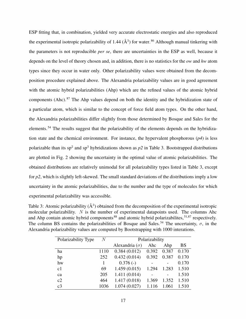
Table 3: Atomic polarizability (Å3) obtained from the decomposition of the experimental isotropicmolecular polarizability. N is the number of experimental datapoints used. The columns Ahcand Ahp contain atomic hybrid components88 and atomic hybrid polarizabilites,51,87 respectively.The column BS contains the polarizabilities of Bosque and Sales.54 The uncertainty, σ, in theAlexandria polarizability values are computed by Bootstrapping with 1000 interations.

Polarizability Type N PolarizabilityAlexandria (σ) Ahc Ahp BS

ha 1110 0.384 (0.012) 0.392 0.387 0.170hp 252 0.432 (0.014) 0.392 0.387 0.170hw 1 0.376 (-) - - 0.170c1 69 1.459 (0.015) 1.294 1.283 1.510ca 205 1.411 (0.014) - - 1.510c2 464 1.417 (0.018) 1.369 1.352 1.510c3 1036 1.074 (0.027) 1.116 1.061 1.510

17

Polarizability Type N PolarizabilityAlexandria (σ) Ahc Ahp BS

na 28 0.863 (0.078) - - 1.050n 147 0.928 (0.023) 1.077 0.964 1.050no 14 1.657 (0.063) - - 1.050ow 1 0.689 (-) - - 0.570o 420 0.565 (0.010) 0.780 0.637 0.570f 68 0.415 (0.016) 0.527 0.296 0.220p4 7 2.214 (0.060) - - 2.480p2 8 3.044 (0.314) - - 2.480s 71 2.932 (0.041) 3.056 3.000 2.990cl 105 2.307 (0.013) 2.357 2.315 2.160br 42 3.441 (0.023) 3.541 3.013 3.290i 17 5.459 (0.090) 5.573 5.415 5.450

0 1 2 3 4 5 6α(Å3)

Rel

ativ

e Fr

eque

ncy

(a.u

.)

ha

o

hp

f

na

n c3

ca c2

c1

no

cl

sp4

p2

br

i

Figure 2: Distribution of atomic polarizabilities. Each distribution was obtained from bootstrap-ping with 1000 iterations. At each iteration, a sample of experimental molecular polarizabilitieswas built randomly with replacement to perform singular value decomposition.

The optimized exponents of Gaussian and Slater density functions are given in Table 4. In these

models, the charge on the core is treated as a point charge and the charge on the shell is treated as

a smeared charge in accord with chemical intuition. The exponent of the valance Slater s-orbital

is optimized for all the atom types, except for bromine and iodine. For these atoms, a Slater 3s

orbital is optimized rather than the valence orbital (See THEORY).

18

Table 4: The optimized exponent for the polarizable Gaussian and Slater s-type orbitals representedby β and ζ in nm−1, rescpectively. Slater 3s orbital has been optimized rather than the valenceSlater s-orbital for Bromine and Iodine (See THEORY).

Polarizability Type β(σ) ζ(σ)ha 12.05 (0.04) 21.39 (0.08)hp 11.81 (0.08) 22.03 (0.33)hw 11.08 (0.01) 16.81 (0.01)c1 9.43 (0.22) 23.34 (0.41)c2 9.74 (0.05) 23.68 (0.17)ca 9.58 (0.03) 23.36 (0.06)c3 12.12 (0.01) 32.88 (0.01)n 10.18 (0.11) 24.88 (0.28)na 11.25 (0.89) 24.39 (0.41)no 9.28 (0.13) 22.82 (0.54)o 11.30 (0.11) 28.86 (0.50)ow 19.31 (0.16) 42.28 (0.01)f 11.75 (0.07) 29.28 (0.33)p2 7.60 (0.08) 20.64 (0.02)p4 7.45 (0.41) 20.64 (0.21)s 7.80 (0.09) 23.77 (0.28)cl 9.70 (0.17) 27.44 (0.19)br 8.96 (1.85) 22.11 (0.76)i 7.68 (0.78) 22.88 (0.39)

Atomic Charges

Fig. 3 displays histograms of the atomic partial charges generated using electrostatic potential

fitting for 2070 molecules from the Alexandria library. The generated charges are chemically

intuitive for most of the atom types. For instances, the charges assigned to oxygen are negative in

most molecules, except for special cases such as (the positive) nitronium ion, nitrosyl bromide, N-

oxonitramide, where oxygen has a small positive charge. However, the algorithm often generates a

negative charge for hydrogens that are connected to aliphatic carbons, denoted by ha atom type in

Fig. 3 and the distribution for carbon atoms are unreasonably wide as well. This is indeed a known

problem of the ESP-fitting algorithm in general which leads to buried atoms, away from the ESP

grid points, becoming a sync for the fitting algorithm, since they contribute little to the ESP.32

19

-1 -0.5 0 0.5 1

ha

-1 -0.5 0 0.5 1

hp

-1 -0.5 0 0.5 1

c1

-1 -0.5 0 0.5 1

ca

-1 -0.5 0 0.5 1

c2

-1 -0.5 0 0.5 1

c3

-1 -0.5 0 0.5 1

na

-1 -0.5 0 0.5 1

n

-1 -0.5 0 0.5 1

no

-1 -0.5 0 0.5 1

o

-1 -0.5 0 0.5 1

f

-1 -0.5 0 0.5 1

p4

-1 -0.5 0 0.5 1

p2

-1 -0.5 0 0.5 1

s

-1 -0.5 0 0.5 1q (e)

cl

-1 -0.5 0 0.5 1q (e)

br

-1 -0.5 0 0.5 1q (e)

i

Figure 3: Histogram of atomic partial charges.

Molecular Polarizability

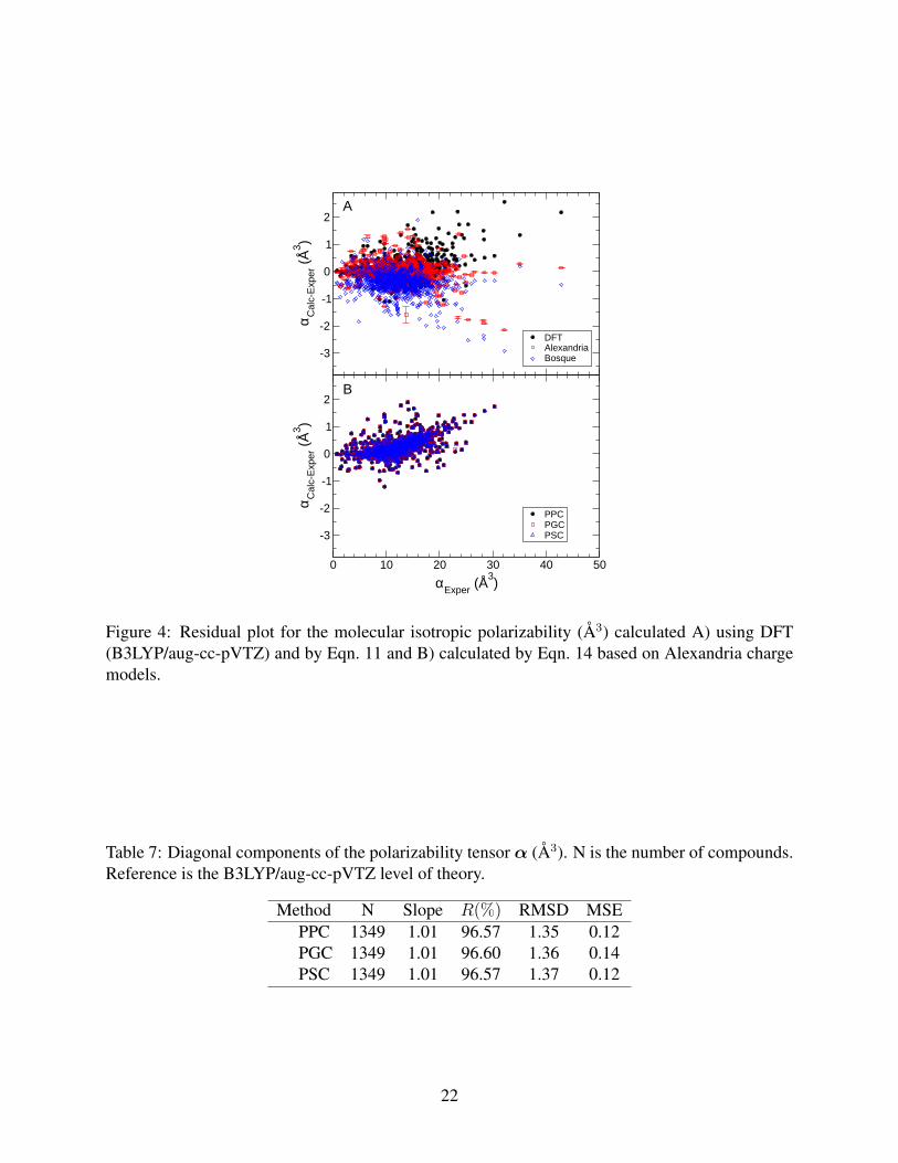
The obtained atomic polarizabilities were evaluated by computing molecular isotropic polarizabil-

ities using Eqn. 11 (Fig. 4A). Table 5 shows that the additive approach used in Alexandria results

in slightly lower RMSD than B3LYP/aug-cc-pVTZ. This can be explained, in part, by the fact

that B3LYP/aug-cc-pVTZ overestimates the dipole polarizability of conjugated molecules such as

tetracene, phenazine, and chrysene due to the presence of delocalized π-electron clouds. The di-

agnosis of the polarizability of delocalized electron densities is beyond the scope of this paper and

has been discussed in detail elsewhere.53,55,89–91 The additive approach is ignorant of the electron

delocalization due to being a simple linear fit, and thus, results in a lower RMSD (0.30 Å3) than

for B3LYP/aug-cc-PVTZ (0.37 Å3). However, it cannot be determined how well the additive ap-

proach works for compounds outside the training set. The results also indicate that Alexandria has

lower RMSD for the molecular isotropic polarizabilities than for Bosque et al.54 (RMSD = 0.58

Å3) (Table 5). This can be explained by the fact the Alexandria has more polarizability types than

20

elements.

The polarizability tensor was computed for all compounds using Eqn. 13 by applying electric

fields with a strength of 10 Vnm−1 in the x, y and z directions and optimizing the shell positions.

The non-additive isotropic polarizability was then calculated using Eqn. 14 and compared to exper-

imental data (Fig. 4B). The RMSD values obtained for the Alexandria charge models are very close

to the RMSD value for B3LYP/aug-cc-pVTZ (Table 6). The MSE values show that the systematic

errors correspond to less than 2% of the average α. The diagonal elements of the polarizability

tensor were compared to the B3LYP calculations (Table 7). Aromatic, conjugated, and annelated

compounds were excluded from the statistics for reasons outlined above. The statistics show a

good agreement between the Alexandria polarizable charge models and the B3LYP/aug-cc-pVTZ

level of theory, even though the RMSD is slightly larger than for the isotropic (the average of the

diagonal components) polarizability.

Table 5: Isotropic polarizability α (Å3) calculated using Eqn. 11 and quantum-mechanically(B3LYP/aug-cc-pVTZ). N is the number of molecules. Reference is experimental data.92,93

Method N slope R(%) RMSD MSEDFT 1168 1.025 99.70 0.37 0.04Alexandria 1168 0.993 99.77 0.30 0.00Bosque 1168 0.982 99.55 0.58 -0.40

Table 6: Isotropic polarizability α (Å3) calculated using Eqn. 14 and quantum-mechanically(B3LYP/aug-cc-pVTZ). N is the number of compounds. Reference is experimental data.92,93

Method N Slope R(%) RMSD MSEDFT 1150 1.01 99.70 0.36 0.05PPC 1150 1.03 99.80 0.46 0.28PGC 1150 1.02 99.80 0.46 0.28PSC 1150 1.02 99.80 0.45 0.27

21

-3

-2

-1

0

1

2

α Cal

c-Ex

per (Å

3 )

DFTAlexandriaBosque

0 10 20 30 40 50αExper (Å

3)

-3

-2

-1

0

1

2

α Cal

c-Ex

per (Å

3 )

PPCPGCPSC

A

B

Figure 4: Residual plot for the molecular isotropic polarizability (Å3) calculated A) using DFT(B3LYP/aug-cc-pVTZ) and by Eqn. 11 and B) calculated by Eqn. 14 based on Alexandria chargemodels.

Table 7: Diagonal components of the polarizability tensor α (Å3). N is the number of compounds.Reference is the B3LYP/aug-cc-pVTZ level of theory.

Method N Slope R(%) RMSD MSEPPC 1349 1.01 96.57 1.35 0.12PGC 1349 1.01 96.60 1.36 0.14PSC 1349 1.01 96.57 1.37 0.12

22

Dipole and Quadrupole Moments of Isolated Molecules

Table 8 compares the predicted total dipole moment to experimental data for rigid molecules only,

as the impact of the vibrational averaging over the accessible conformations of flexible molecules

is expected to be significant. “Rigid molecules” were those determined to have no rotatable bonds.

The RMSD and MSE values indicate that the predicted accuracy for total dipole moments by

Alexandria polarizable charges is the same as that for B3LYP/aug-cc-pVTZ level of theory. The

scattering of residuals obtained from this comparison is homogenous, indicating that the error in

predicting the total dipole moment is not systematic (Fig. 5). Due to the lack of experimental data,

the accuracy of the Alexandria charge models in computing the components of the dipole vector

and the diagonal elements of the quadruple tensor was evaluated by comparing to the B3LYP calcu-

lations (Table 9). Here, the comparison is carried out for all molecules, both rigid and flexible. The

results display that the dipole components along the x, y and z directions predicted by Alexandria

charge models are in excellent agreement with the B3LYP calculations. The quadrupole tensor

components (Table 10), on the other hand, are underestimated in comparison to DFT, while the

RMSD values are consistent with previous studies.94

Table 8: Total dipole moment µ (Debye). N is the number of compounds. Reference is experimen-tal data.92,93

Method N Slope R(%) RMSD MSEDFT 478 1.05 98.10 0.30 0.08PPC 478 1.05 98.10 0.31 0.10PGC 478 1.04 97.70 0.32 0.09PSC 478 1.04 98.00 0.31 0.08

Table 9: Components of the dipole vector µ (Debye). N is the number of compounds. Referenceis the B3LYP/aug-cc-pVTZ level of theory.

Method N Slope R(%) RMSD MSEPPC 1349 0.98 99.70 0.16 0.00PGC 1349 0.98 99.70 0.15 0.00PSC 1349 0.98 99.67 0.17 0.00

23

Table 10: Diagonal components of the quadrupole tensor θ (Buckingham). N is the number ofcompounds. Reference is the B3LYP/aug-cc-pVTZ level of theory.

Method N Slope R(%) RMSD MSEPPC 1349 1.55 96.73 2.23 -0.05PGC 1349 1.55 96.53 2.25 -0.06PSC 1349 1.55 95.77 2.32 -0.06

0 1 2 3 4 5 6 7µExperiment (Debye)

-1.5

-1

-0.5

0

0.5

1

1.5

µ Cal

c-Ex

perim

ent (D

ebye

)

DFTPPCPGCPSC

Figure 5: Residual plot of total molecular dipole moment (Debye) from DFT (B3LYP/aug-cc-pVTZ) and Alexandria charge models.

24

Dipole Moment of Dimers and Clusters

The Alexandria polarizable charge models were validated by computing the components of the

dipole vector for different sets of homo- and hetero-dimers of common organic molecules and

water clusters up to 10 monomers (Table 1). We also carried out the same calculations with fixed

point charges without polarization (derived from an ESP fit and denoted here by PC) because this

is widely used in empirical force fields such as GAFF,72 OPLS (Optimized Potential for Liquid

Simulations),95 and CGenFF (CHARMM General Force Field).96

The total RMSD from DFT dipole moments decreases going from the fixed point charge model

to polarizable charges by more than 50% (Table 11). The scattering of the residuals indicates that

the error is random for the polarizable charges, while it is systematic for the fixed point charge

(Fig. 6).

The results show that the polarizable point charge is as accurate as the polarizable smeared

charges in predicting the dipole moments of the dimers at the equilibrium geometry. For the water

clusters, the RMSD was found to be 0.07 and 0.04 (Debye) for the PC and PPC models respectively.

In contrast, for popular fixed-charge models such as TIP3P97 or SPC/E,98 which have monomer

dipoles of the order of 2.3 Debye instead of the experimental 1.85 Debye, a dimer dipole moment of

3.8 (Debye) is found for the water dimer,4,84 which deviates significantly from 2.4 to 2.7 (Debye)

measured experimentally.99 Fig. 7 shows the total dipole moment of a water dimer at different

separations along the hydrogen bond-breaking coordinates. Both PC and PPC fail to reproduce the

dipole moment at short distances, while PGC and PSC are in good agreement with the B3LYP/aug-

cc-pVTZ level of theory. The RMSD averaged over 191 conformations of the water dimer is 0.40

for PC, 0.24 for PPC, and ∼0.04 (Debye) for both PGC and PSC. However, further evaluations of

other properties of water clusters, e.g. the vibrational spectra100 and exchange repulsion101 would

be needed to scrutinize the effect of the water atomic charge distributions more rigorously.

The performance of the Alexandria charge models was also compared for different non-covalent

interactions stabilizing homo- and hetero-dimer of organic compounds (Table 12). Consistently,

the polarizable charges displayed a better performance than the PC. The results also exhibit that the

25

RMSD value obtained for the halogen bond and halogen-π interactions are higher than the other

types of interactions for all the charge models compared in Table 12.

Table 11: Root-mean square deviation for Alexandria charge models from QM dipole vector µcomponents (Debye) at the B3LYP/aug-cc-pVTZ level of theory.

Model S66 X40 SHBC Water TotalPC 0.21 0.29 0.18 0.07 0.20PPC 0.05 0.17 0.12 0.04 0.08PGC 0.06 0.17 0.11 0.05 0.09PSC 0.06 0.16 0.11 0.06 0.09

Table 12: Root-mean square deviation for Alexandria charge models from QM dipole vector µcomponents (Debye) at the B3LYP/aug-cc-pVTZ level of theory for specific interactions. N is thenumber of dimers

Interaction N PC PPC PGC PSCπ − π 6 0.10 0.01 0.03 0.02Halogen-π 4 0.41 0.24 0.25 0.23OH-π 4 0.16 0.12 0.11 0.11Halogen bond 20 0.23 0.29 0.20 0.23Hydrogen bond 10 0.49 0.12 0.12 0.11Dispersion 4 0.15 0.13 0.13 0.13Induction 4 0.06 0.05 0.05 0.05T-Shaped Aromatic Dimers 4 0.26 0.05 0.01 0.03

26

-8 -6 -4 -2 0 2 4 6 8µ Electronic (Debye)

-2

-1

0

1

2

µ Cal

c-El

ectro

nic (D

ebye

)

PCPPCPGCPSC

Figure 6: Residual plot of the components of the dipole vector obtained for homo- and hetero-dimers and water clusters using Alexandria charge models.

0.1 0.15 0.2 0.25 0.3 0.35 0.4 0.45 0.5O---H Distance (nm)

2

2.5

3

3.5

4

4.5

5

5.5

6

µ (D

ebye

)

DFTPCPPCPGCPSC

Figure 7: Total dipole moment (Debye) for water dimer.

27

Electrostatic Interaction Energy of Water Dimer

Fig. 8 plots the electrostatic component of the interaction energy (Eelec) for the water dimer along

the hydrogen bond-breaking coordinate using SAPT2+/aug-cc-pVTZ and the Alexandria charge

models. The O · · · H distance is varied from 0.12 to 0.5 nm. Our quantum calculations find Eelec

to be -33.11 kJ/mol at the equilibrium distance (0.196 nm) in the aug-cc-pVTZ basis, which is

consistent with -30.25, -34.01 and -35.18 (kJ/mol) reported in other studies at different high levels

of theory.12,102,103 The variation between these values somehow reflects the uncertainty in quantum

chemistry methods in computing intermolecular interaction energies due to different levels of the-

ory. We find Eelec to be -17.93 for PC, -25.06 for PPC, -31.65 for PGC, and -32.58 (kJ/mol) for

PSC at the equilibrium geometry. The RMSD averaged over 191 conformations of the water dimer

is 24.62 for PC, 18.15 for PPC, 1.93 for PGC, and 1.60 (kJ/mol) for PSC. This shows that the devi-

ation from the SAPT2+ electrostatic interaction energy systematically decreases with increasingly

realistic charge models, in agreement with previous studies.12,94

0.1 0.15 0.2 0.25 0.3 0.35 0.4 0.45 0.5O--H Distance (nm)

-400

-350

-300

-250

-200

-150

-100

-50

0

E ele

c (kJ/

mol

)

SAPT2+PCPPCPGCPSC

Figure 8: Electrostatic interaction energy (kJ/mol) for water dimer.

28

DISCUSSION

The importance of using polarization and damped (smeared) Coulomb interactions in molecular

mechanics force fields has been pointed out in a number of previous studies.2,8,9,12,17,19 However,

modeling of molecular polarizability requires a description of the atomic polarizability, which

cannot be determined experimentally.50 Using smeared charge models such as Gaussian and Slater

s-type atomic orbitals also require determining the exponents of the orbitals. As a result, atomic po-

larizabilities and orbital exponents expand the parameter space of empirical force fields somewhat,

by two parameters per atom. In order for force fields to be transferable it is therefore important to

validate that these parameters can be determined by the atom type alone, which is what we attempt

in this paper. It is possible that the introduction of more accurate physics in the molecular models

will reduce the need for having so many atom types as if common in most force fields, but this

remains to be determined.

The most widely used Drude polarizable force field is likely polarizable CHARMM.6,42,104 It

treats atomic partial charges as point charges. The sign of the charge is chosen to be positive on the

core—representing the nucleus—and negative on the Drude—representing the electron cloud—to

be intuitively consistent. In order to reduce the number of shell particles and to avoid the polar-

ization catastrophe, polarizable CHARMM assigns polarizability only to non-hydrogen atoms and

damps the electrostatic 1-2 and 1-3 pair interactions.6,42,104 To compensate for this, polarizabilities

are scaled down by 15%,42 but in addition anisotropic polarizabilities are used for oxygen atoms in

e.g. carbonyl groups,104 as introduced for water early on.4 It has been shown though, that assigning

polarizability to hydrogens improves the description of the water polarization and allows to use the

full molecular polarizability rather than scaling it down.105 Moreover, the atomic polarizability of

0.432 and 0.384 Å3 obtained in this study for polar and non polar hydrogens, respectively, sug-

gest that hydrogens contribute significantly to the molecular polarizability. The AMOEBA force

field assigns a polarizability of 0.496 Å3 to hydrogens7 which is similar to our values. Drude

polarizable Gaussian charges have been developed for specific organic molecules such as carbon

dioxide20 and water.24 In these models, some shells have a positive charge and some others have

29

a negative charge and all the cores are neutral, which is counter-intuitive. Rappé and Goddard

applied the fluctuating charge method to describe polarizability of Slater charge densities.15 The

major problem with the fluctuating charge method is that it does not describe the out-of-plane

polarization.1 To circumvent this shortcoming, Donchev et al. parametrized a Drude model with

Slater charges on a small set of monomers and dimers.94 Other Slater charge models are, to our

knowledge, non-polarizable.2,12,17,19,29 Therefore, the main goal in this paper was to build a Drude

model with s-type Gaussian and Slater density functions. We attempted to provide a general and

robust platform to determine the values of atomic polarizabilities and to optimize the exponent of

1s-Gaussian and ns-Slater (n = 1, 2, 3) orbitals for H, C, N, O, P, S and halogens (F, Cl, Br, I) to

be transferable among organic molecules.

Analysis of the polarizabilities, dipoles, and quadrupoles obtained for the large number of

molecules used in this study strongly suggests that the atomic polarizabilities and the exponents

of the spherical Gaussian and Slater density functions are transferable among the molecules used

and are likely to be transferable beyond the Alexandria library. We found that both the addi-

tive (Eqn. 11) and the non-additive (Eqn. 14) approaches to calculating the molecular isotropic

polarizability yielded results in agreement with the reference data for the molecules used. This

conclusion, however, is not entirely general because the non-additive effects of conjugated chains

with multiple double bonds was not addressed in this work, mainly due to systematic errors in

the applied density functional theory method.55 A recently developed approach to decompose the

linear response properties into additive and cooperative contributions can be used to quantify the

non-additive effects in the polarizability of conjugated chains.106

Evaluation of the charge models on dimers and complexes showcases the poor performance

of the point charge model in predicting the dipole vector of the homo- and hetero-dimer of or-

ganic molecules. The explicit inclusion of the charge polarization decreased the RMSD from the

B3LYP/aug-cc-pVTZ calculations by∼50% (Table 11). A similar improvement can be anticipated

for simulating the liquid phase, however, the error may accumulate and/or cancel accross multiple

interacting dimers in the liquid phase. Polarizable charges significantly decreased the deviation

30

from the components of the dipole vector calculated at the B3LYP/aug-cc-pVTZ level of theory

for dimers stabilized by hydrogen bonding and π − π stacking, which are the main non-covalent

interactions stabilizing secondary and tertiary structures of nucleic acids. However, in the case of

halogen bonding, the RMSD is relatively high even though the RMSD obtained for the polarizable

charges was much smaller than the fixed point charge (Table 12). Halogen bonding is important

in molecular recognition, because about half of the drugs or drug-like compounds contain fluo-

rine and chlorine.107,108 Therefore, the presented polarizable models need to be improved further

to describe the “σ hole” in halogen bonds. One possible solution is to go beyond atomic centers

through off-center virtual sites.104 Among the widely used force fields, OPLS was first to explicitly

treat the “σ hole” in halogen bonds by defining a massless virtual site (X-site) carrying a positive

charge on Cl, Br, and I.109 Similar extensions were introduced into the CHARMM Generalized

Force Field110 and the Polarizable CHARMM force field.85

We found that the polarizable point charge is as accurate as the polarizable Gaussian and Slater

charges for reproducing the dipole vector and the diagonal elements of the polarizability- and

quadrupole tensors of the isolated molecules in the gas phase. This is consistent with the fact

that the interactions at short intramolecular distances are excluded in our force field calculations

to attenuate the quantum mechanical effect. In order to study the charge penetration effect at

short distances, the electrostatic interaction energy and the total dipole moment were calculated

for 191 conformations of a water dimer at separation distances from 0.12 to 0.5 nm. Consistent

with previous studies,12,17 we find that the polarizable point charge fails to describe both the dipole

moment (Fig. 7) and the electrostatic energy (Fig. 8) at very short distances. The results also

showed that, although all the polarizable charges accurately predicted the dipole moment of the

water dimer at equilibrium geometry, the PPC model deviated from the reference electrostatic

energy of the equilibrium geometry by as much as 8.05 (kJ/mol), while the deviation was 1.46

(kJ/mol) for PGC and 0.53 (kJ/mol) for PSC. This suggests that the charge penetration effect is

needed in addition to the charge polarization to yield accurate electrostatic energies even at the

equilibrium distance.

31

In summary, the atomic polarizabilities and the exponents of the s-type Gaussian and Slater

density functions presented in this work reproduce electrostatic properties for molecules of the

Alexandria library and are likely transferable to other compounds with similar chemistries. Al-

though, the Alexandria polarizable point charge is accurate enough to be used for prediction of

the isotropic polarizability and dipole moments of organic molecules in the gas phase, this work

strongly suggests that the atomic partial charges in molecular dynamics simulations should be

treated as smeared charges to produce accurate electrostatic energies, particularly when simulating

the condensed phase.

32

Acknowledgments

The Swedish research council is acknowledged for financial support to DvdS (grant 2013-5947)

and for a grant of computer time (SNIC2016/34-44) through the High Performance Computing

Center North in Umeå, Sweden. The Helmholtz Association through the Center for Free-Electron

Laser Science at DESY is acknowledged as well.

Graphical TOC Entry

H2O

2-ψ

Gaussian Slater

References

(1) Cieplak, P.; Dupradeau, F.-Y.; Duan, Y.; Wang, J. J. Phys. Condens. Matter 2009, 21,

333102.

(2) Wang, B.; Truhlar, D. G. J. Chem. Theory Comput. 2010, 6, 3330–3342.

(3) Jordan, P. C.; van Maaren, P. J.; Mavri, J.; van der Spoel, D.; Berendsen, H. J. C. J. Chem.

Phys. 1995, 103, 2272–2285.

(4) van Maaren, P. J.; van der Spoel, D. J. Phys. Chem. B. 2001, 105, 2618–2626.

(5) Ren, P.; Ponder, J. W. J. Comput. Chem. 2002, 23, 1497–1506.

(6) Anisimov, V. M.; Lamoureux, G.; Vorobyov, I. V.; Huang, N.; Roux, B.; MacKerell,

Jr., A. D. J. Chem. Theory Comput. 2005, 1, 153–168.

33

(7) Ponder, J. W.; Wu, C.; Ren, P.; Pande, V. S.; Chodera, J. D.; Schnieders, M. J.; Haque, I.;

Mobley, D. L.; Lambrecht, D. S.; DiStasio Jr., R. A.; Head-Gordon, M.; Clark, G. N. I.;

Johnson, M. E.; Head-Gordon, T. J. Phys. Chem. B 2010, 114, 2549–2564.

(8) Ahlström, P.; Wallqvist, A.; Engström, S.; Jönsson, B. Mol. Phys. 1989, 68, 563–581.

(9) Thole, B. T. Chem. Phys. 1981, 59, 341–345.

(10) Lindan, P. J. D. Mol Simul 1995, 14, 303–312.

(11) Allen, M. P.; Tildesley, D. J. Computer Simulation of Liquids, 2nd ed.; Oxford Science

Publications: Oxford, 2017.

(12) Wang, Q.; Rackers, J. A.; He, C.; Qi, R.; Narth, C.; Lagardere, L.; Gresh, N.; Ponder, J. W.;

Piquemal, J.-P.; Ren, P. J. Chem. Theory Comput. 2015, 11, 2609–2618.

(13) Hall, G. G.; Tsujinaga, K. Theor. Chim. Acta. 1986, 69, 425–436.

(14) Hall, G. G.; Smith, C. M. Theor. Chim. Acta. 1986, 69, 71–81.

(15) Rappé, A. K.; Goddard III, W. A. J. Phys. Chem. 1991, 95, 3358–3363.

(16) Kiss, P. T.; Sega, M.; Baranyai, A. J. Chem. Theory Comput. 2014, 10, 5513–5519.

(17) Öhrn, A.; Hermida-Ramon, J. M.; Karlström, G. J. Chem. Theory Comput. 2016, 12, 2298–

2311.

(18) Wang, F.-F.; Kumar, R.; Jordan, K. D. Theor. Chem. Acc. 2012, 131, 1132.

(19) Wang, B.; Truhlar, D. G. J. Chem. Theory Comput. 2014, 10, 4480–4487.

(20) Jiang, H.; Moultos, O. A.; Economou, I. G.; Panagiotopoulos, A. Z. J. Phys. Chem. B 2016,

120, 984–994.

(21) Kiss, P. T.; Baranyai, A. J. Chem. Phys. 2014, 141, 114501.

34

(22) Baranyai, A.; Kiss, P. T. J. Chem. Phys. 2010, 133, 144109.

(23) Baranyai, A.; Kiss, P. T. J. Chem. Phys. 2011, 135, 234110.

(24) Kiss, P. T.; Baranyai, A. J. Chem. Phys. 2012, 137, 84506–84508.

(25) Elking, D.; Darden, T.; Woods, R. J. J. Comput. Chem. 2007, 28, 1261–1274.

(26) Ghahremanpour, M. M.; van Maaren, P.; van der Spoel, D. Alexandria Library [Data set].

Zenodo. 2017; http://doi.org/10.5281/zenodo.1004711.

(27) Ghahremanpour, M. M.; van Maaren, P. J.; van der Spoel, D. Sci. Data 2018, 5, 180062.

(28) Cailliez, F.; Pernot, P. J. Chem. Phys. 2011, 134, 054124.

(29) Verstraelen, T.; Vandenbrande, S.; Heidar-Zadeh, F.; Vanduyfhuys, L.; Van Speybroeck, V.;

Waroquier, M.; Ayers, P. W. J. Chem. Theory Comput. 2016, 12, 3894–3912.

(30) Murray, J. S.; Politzer, P. Wiley Interdiscip. Rev. Comput. Mol. Sci. 2011, 1, 153–163.

(31) Besler, B. H.; Merz Jr., K. M.; Kollman, P. A. J. Comput. Chem. 1990, 11, 431–439.

(32) Sigfridsson, E.; Ryde, U. J. Comput. Chem. 1998, 19, 377–395.

(33) Rick, S. W.; Stuart, S. J.; Berne, B. J. J. Chem. Phys. 1994, 101, 6141–6156.

(34) Hentschke, R.; Aydt, E. M.; Fodi, B.; Schöckelmann, E. Molekulares Modellieren mit Kraft-

feldern; Bergische Universität Wuppertal: Wuppertal, Germany, 2004.

(35) Guseinov, I. I. J. Phys. B: Atom. Molec. Phys. 1970, 3, 1399.

(36) Elking, D. M.; Cisneros, G. A.; Piquemal, J.-P.; Darden, T. A.; Pedersen, L. G. J. Chem.

Theory Comput. 2010, 6, 190–202.

(37) Dick, B. G.; Overhauser, A. W. Phys. Rev. 1958, 112, 90–103.

35

(38) Saint-Martin, H.; Hernández-Cobos, J.; Bernal-Uruchurtu, M. I.; Ortega-Blake, I.; Berend-

sen, H. J. C. J. Chem. Phys. 2000, 113, 10899–10912.

(39) Lamoureux, G.; Roux, B. J. Phys. Chem. 2003, 119, 3025–3039.

(40) Geerke, D. P.; van Gunsteren, W. F. J. Chem. Theory Comput. 2007, 3, 2128–2137.

(41) Lopes, P. E. M.; Lamoureux, G.; Roux, B.; MacKerell, Jr., A. D. J. Phys. Chem. B. 2007,

111, 1.

(42) Lopes, P. E. M.; Huang, J.; Shim, J.; Luo, Y.; Li, H.; Roux, B.; MacKerell, J., Alexander D.

J. Chem. Theory Comput 2013, 9, 5430–5449.

(43) Lemkul, J.; Roux, B.; van der Spoel, D.; MacKerell, A. J. Comput. Chem. 2015, 36, 1473–

1479.

(44) Albaugh, A.; Head-Gordon, T. J. Chem. Theory Comput. 2017, 13, 5207–5216.

(45) Huang, J.; Simmonett, A. C.; Pickard IV, F. C.; MacKerell Jr., A. D.; Brooks, B. R. J. Chem.

Phys. 2017, 147, 161702.

(46) Li, A.; Voronin, A.; Fenley, A. T.; Gilson, M. K. J. Phys. Chem. B 2016, 120, 8668–8684.

(47) Chialvo, A. A.; Moucka, F.; Vlcek, L.; Nezbeda, I. J. Phys. Chem. B 2015, 119, 5010–5019.

(48) Lindan, P. J. D.; Gillan, M. J. J. Phys.: Condens. Matter 1993, 5, 1019–1030.

(49) Lemkul, J. A.; Huang, J.; Roux, B.; MacKerell, A. D. Chem. Rev. 2016, 116, 4983–5013.

(50) Silberstein, L. Philos. Mag. 1917, 33, 92–128.

(51) Kang, Y. K.; Jhon, M. S. Theor. Chem. Acc. 1982, 61, 41–48.

(52) McMeekin, T. L.; Groves, M. L.; Wilensky, M. Biochem. Biophys. Res. Commun. 1962, 7,

151–160.

36

(53) Alparone, A. Chem. Phys. 2013, 410, 90 – 98.

(54) Bosque, R.; Sales, J. J. Chem. Inf. Comput. Sci. 2002, 42, 1154–1163.

(55) Limacher, P. A.; Mikkelsen, K. V.; Lüthi, H. P. J. Chem. Phys. 2009, 130, 194114.

(56) Alipour, M. J. Phys. Chem. A 2014, 118, 5333–5342.

(57) Ghahremanpour, M. M.; van Maaren, P. J.; Ditz, J.; Lindh, R.; van der Spoel, D. J. Chem.

Phys. 2016, 145, 114305.

(58) Hohenberg, P.; Kohn, W. Phys. Rev. 1964, 136, B864–B871.

(59) Becke, A. D. Phys. Rev. A 1988, 38, 3098–3100.

(60) Lee, C.; Yang, W.; Parr, R. G. Phys. Rev. B 1988, 37, 785–789.

(61) Becke, A. D. J. Chem. Phys. 1993, 98, 5648–5652.

(62) Kendall, R. A.; Dunning, Jr., T. H.; Harrison, R. J. J. Chem. Phys. 1992, 96, 6796–6806.

(63) Woon, D. E.; Dunning, Jr., T. H. J. Chem. Phys. 1993, 99, 1914–1929.

(64) Woon, D. E.; Dunning, Jr., T. H. J. Chem. Phys. 1993, 98, 1358–1371.

(65) Rezác, J.; Riley, K. E.; Hobza, P. J. Chem. Theory Comput. 2011, 7, 2427–2438.

(66) Rezác, J.; Riley, K. E.; Hobza, P. J. Chem. Theory Comput. 2014, 10, 1359–1360.

(67) Rezác, J.; Riley, K. E.; Hobza, P. J. Chem. Theory Comput. 2012, 8, 4285–4292.

(68) Riley, K. E.; Hobza, P. J. Chem. Theory Comput. 2008, 4, 232–242.

(69) Temelso, B.; Archer, K. A.; Shields, G. C. J. Phys. Chem. A. 2011, 115, 12034–12046.

(70) O’Boyle, N. M.; Banck, M.; James, C. A.; Morley, C.; Vandermeersch, T.; Hutchison, G. R.

J. Cheminf. 2011, 3, 33.

37

(71) SMARTS - A Language for Describing Molecular Patterns.

http://www.daylight.com/dayhtml/doc/theory/theory.smarts.html, 2008.

(72) Wang, J.; Wolf, R. M.; Caldwell, J. W.; Kollman, P. A.; Case, D. A. J. Comput. Chem. 2004,

25, 1157–1174.

(73) Case, D. et al. AMBER 2016. 2016; University of California, San Francisco.

(74) Bayly, C. I.; Cieplak, P.; Cornell, W. D.; Kollman, P. A. J. Phys. Chem. 1993, 97, 10269–

10280.

(75) Cerutti, D. S.; Swope, W. C.; Rice, J. E.; Case, D. A. J. Chem. Theory Comput. 2014, 10,

4515–4534.

(76) Pronk, S.; Páll, S.; Schulz, R.; Larsson, P.; Bjelkmar, P.; Apostolov, R.; Shirts, M. R.;

Smith, J. C.; Kasson, P. M.; van der Spoel, D.; Hess, B.; Lindahl, E. Bioinformatics 2013,

29, 845–54.

(77) Freedman, D. A. Ann. Stat. 1981, 9, 1218–1228.

(78) Frederiksen, S. L.; Jacobsen, K. W.; Brown, K. S.; Sethna, J. P. Phys. Rev. Lett. 2004, 93,

165501.

(79) Mortensen, J. J.; Kaasbjerg, K.; Frederiksen, S. L.; Nørskov, J. K.; Sethna, J. P.; Jacob-

sen, K. W. Phys. Rev. Lett. 2005, 95, 216401.

(80) Frisch, M. J. et al. Gaussian 16 Revision A.03. 2016; Gaussian Inc. Wallingford CT.

(81) M., T. J. et al. Wiley Interdiscip. Rev. Comput. Mol. Sci. 2, 556–565.

(82) Jeziorski, B.; Moszynski, R.; Szalewicz, K. Chem. Rev. 1994, 94, 1887–1930.

(83) Parker, T. M.; Burns, L. A.; Parrish, R. M.; Ryno, A. G.; Sherrill, C. D. J. Chem. Phys. 2014,

140, 094106.

38

(84) Yu, W.; Lopes, P. E. M.; Roux, B.; MacKerell, Jr., A. D. J. Chem. Phys. 2013, 138, 34508.

(85) Lin, F.-Y.; MacKerell, A. D. J. Chem. Theory Comput. 2018, 14, 1083–1098.

(86) Moelwyn-Hughes, E. A. Physical chemistry, 2nd ed.; Pergamon Press, New York, 1964.

(87) Miller, K. J. J. Am. Chem. Soc. 1990, 112, 8542–8553.

(88) Miller, K. J.; Savchik, J. A. J. Am. Chem. Soc. 1979, 101, 7206–7213.

(89) Rustagi, K.; Ducuing, J. Opt. Commun. 1974, 10, 258 – 261.

(90) Huzak, M.; Deleuze, M. S. J. Chem. Phys. 2013, 138, 024319.

(91) Champagne, B.; Perpête, E. A.; van Gisbergen, S. J. A.; Baerends, E.-J.; Snijders, J. G.;

Soubra-Ghaoui, C.; Robins, K. A.; Kirtman, B. J. Chem. Phys. 1998, 109, 10489–10498.

(92) Lide, D. R. CRC Handbook of Chemistry and Physics 90th edition; CRC Press: Cleveland,

Ohio, 2009.

(93) Rowley, R. L.; Wilding, W. V.; Oscarson, J. L.; Yang, Y.; Giles, N. F. Data Compilation of

Pure Chemical Properties (Design Institute for Physical Properties; American Institute for

Chemical Engineering: New York, 2012.

(94) Donchev, A. G.; Ozrin, V. D.; Subbotin, M. V.; Tarasov, O. V.; Tarasov, V. I. Proc. Natl.

Acad. Sci. U.S.A. 2005, 102, 7829–7834.

(95) Harder, E. et al. J. Chem. Theory Comput. 2016, 12, 281–296.

(96) Vanommeslaeghe, K.; Hatcher, E.; Acharya, C.; Kundu, S.; Zhong, S. J. Comput. Chem.

2010, 31, 671–690.

(97) Jorgensen, W. L. J. Am. Chem. Soc. 1981, 103, 335–340.

(98) Berendsen, H. J. C.; Grigera, J. R.; Straatsma, T. P. J. Phys. Chem. 1987, 91, 6269–6271.

39

(99) Gregory, J. K.; Clary, D. C.; Liu, K.; Brown, M. G.; Saykally, R. J. Science 1997, 275,

814–817.

(100) Jordan, K. D.; Sen, K. Chemical Modelling; The Royal Society of Chemistry, 2017; Vol. 13;

pp 105–131.

(101) Kumar, R.; Wang, F.-F.; Jenness, G. R.; Jordan, K. D. J. Chem. Phys. 2010, 132, 014309.

(102) Glendening, E. D. J. Phys. Chem. A 2005, 109, 11936–11940.

(103) Su, P.; Li, H. J. Chem. Phys. 2009, 131, 014102.

(104) Harder, E.; Anisimov, V. M.; Vorobyov, I. V.; Lopes, P. E. M.; Noskov, S. Y.; MacK-

erell, A. D.; Roux, B. J. Chem. Theory Comput. 2006, 2, 1587–1597.

(105) Schropp, B.; Tavan, P. J. Phys. Chem. B 2008, 112, 6233–6240.

(106) Lambrecht, E., Daniel; Berquist 2018; https://doi.org/10.26434/chemrxiv.

5773968.v1.

(107) Metrangolo, P.; Neukirch, H.; Pilati, T.; Resnati, G. Acc. Chem. Res. 2005, 38, 386–395.

(108) Lu, Y.; Liu, Y.; Xu, Z.; Li, H.; Liu, H.; Zhu, W. Exp. Op. Drug Disc. 2012, 7, 375–383.

(109) Jorgensen, W. L.; Schyman, P. J. Chem. Theory Comput. 2012, 8, 3895–3901.

(110) Soteras-Gutiérrez, I.; Lin, F. Y.; Vanommeslaeghe, K.; Lemkul, J. A.; Armacost, K. A.;

Brooks III, C. L.; MacKerell Jr., A. D. Bioorg. Med. Chem. 2016, 24, 4812âLŠ4825.

40

download fileview on ChemRxivdistributed_charges.pdf (3.41 MiB)