Embed Size (px)
Citation preview
Pointer Analysis – Part I
Mayur Naik
Intel Research, Berkeley
CS294 Lecture
March 17, 2009
Pointer Analysis
• Answers which pointers may point to which memory locations
• Lies at the heart of many program optimization and verification problems
• Problem is undecidable
• But many conservative approximations exist
• Continues to be active area of research
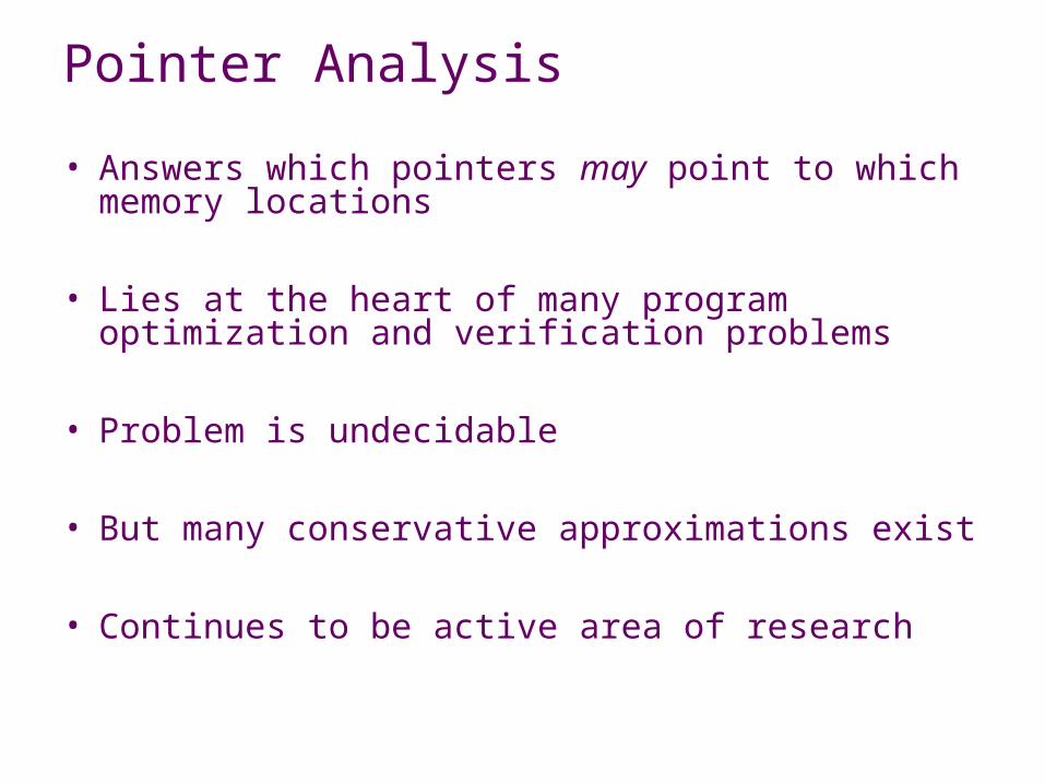
Example Java Programclass Link<T> { T data; Link<T> next;}
class List<T> { T tail; void append(T c) { Link<T> k = new Link<T>(); k.data = c; Link<T> t = this.tail; if (
t.next = k; this.tail = k; }}
t != null)
static void main() { String[] a = new String[] { “a1”, “a2” }; String[] b = new String[] { “b1”, “b2” }; List<String> l; l = new List<String>(); for ( String v1 = a[i]; l.append(v1); } print(l); l = new List<String>(); for ( String v2 = b[i]; l.append(v2); } print(l);}
int i = 0; i < a.length; i++) {
int i = 0; i < b.length; i++) {

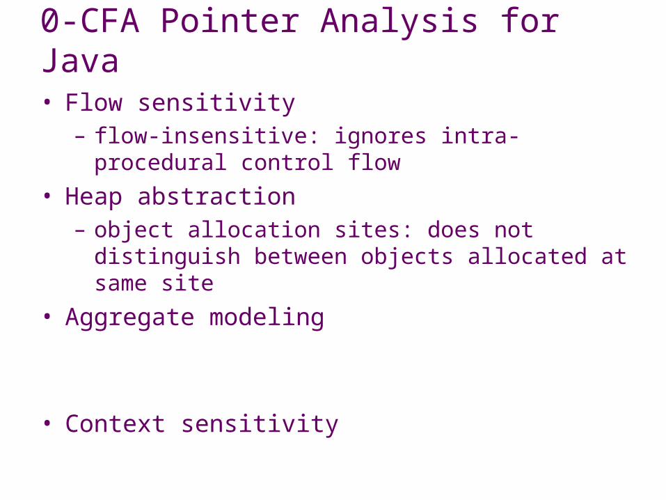
• Flow sensitivity– flow-insensitive: ignores intra-procedural control flow
• Heap abstraction
• Aggregate modeling
• Context sensitivity
0-CFA Pointer Analysis for Java
static void main() { String[] a = new String[] { “a1”, “a2” } String[] b = new String[] { “b1”, “b2” } List<String> l l = new List<String>() for ( String v1 = a[ ] l.append(v1) } l = new List<String>() for ( String v2 = b[ ] l.append(v2) }}
;
;
*
int i = 0; i < a.length; i++) {
int i = 0; i < b.length; i++) {
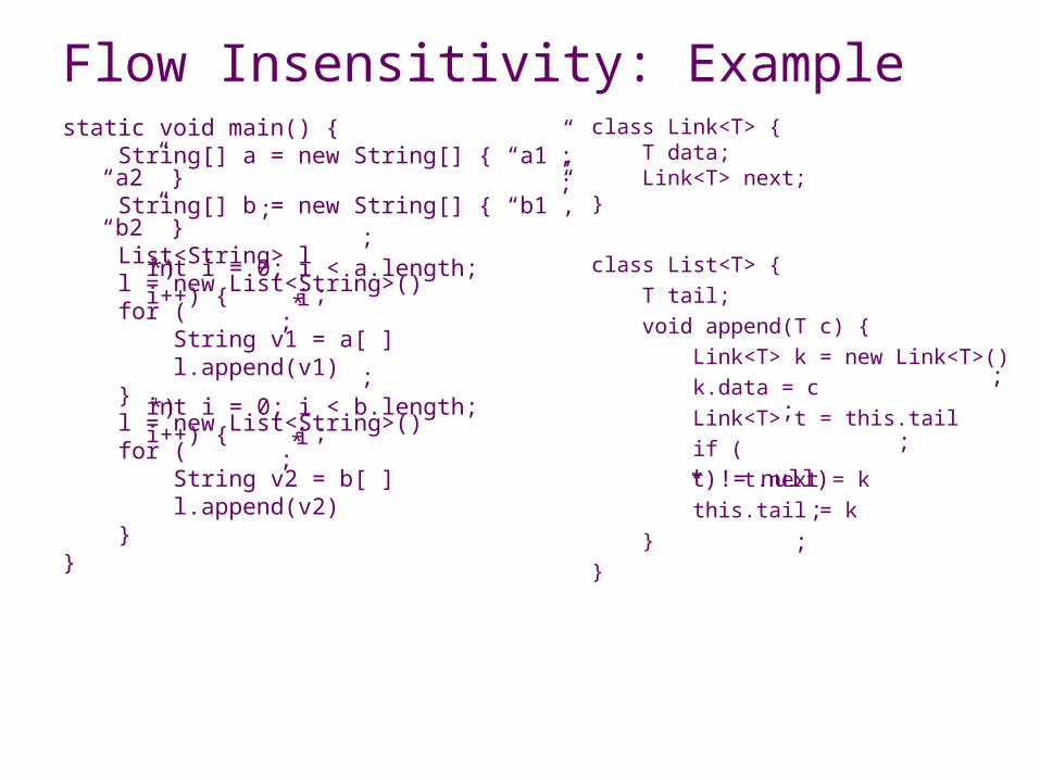
Flow Insensitivity: Exampleclass Link<T> { T data; Link<T> next;}
class List<T> { T tail; void append(T c) { Link<T> k = new Link<T>() k.data = c Link<T> t = this.tail if ( t.next = k this.tail = k }}
;
;
;
;;
;
;
;;
;
*)
*)
t != null)*)
i
i
*
;
;

class List<T> { T tail; void append(T c) { Link<T> k = new Link<T>() k.data = c Link<T> t = this.tail t.next = k this.tail = k }}
static void main() { String[] a = new String[] { “a1”, “a2” }
String[] b = new String[] { “b1”, “b2” }
List<String> l
l = new List<String>() String v1 = a[*]
l.append(v1) l = new List<String>() String v2 = b[*]
l.append(v2)}
Flow Insensitivity: Example

static void main() { String[] a = new String[] { “a1”, “a2” }
String[] b = new String[] { “b1”, “b2” }
List<String> l
l = new List<String>() String v1 = a[*]
l.append(v1) l = new List<String>() String v2 = b[*]
l.append(v2)}
Call Graph (Base Case): Example
Code deemed reachable so far …
class List<T> { T tail; void append(T c) { Link<T> k = new Link<T>() k.data = c Link<T> t = this.tail t.next = k this.tail = k }}
• Flow sensitivity– flow-insensitive: ignores intra-procedural control flow
• Heap abstraction– object allocation sites: does not distinguish between
objects allocated at same site
• Aggregate modeling
• Context sensitivity
0-CFA Pointer Analysis for Java

static void main() { String[] a = new String[] { “a1”, “a2” }
String[] b = new String[] { “b1”, “b2” }
List<String> l
l = new List<String>() String v1 = a[*]
l.append(v1) l = new List<String>() String v2 = b[*]
l.append(v2)}
Heap Abstraction: Example
class List<T> { T tail; void append(T c) { Link<T> k = new Link<T>() k.data = c Link<T> t = this.tail t.next = k this.tail = k }}
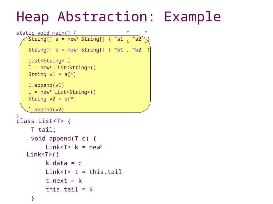
static void main() { String[] a = new1 String[] { “a1”, “a2” }
String[] b = new2 String[] { “b1”, “b2” }
List<String> l
l = new3 List<String>() String v1 = a[*]
l.append(v1) l = new4 List<String>() String v2 = b[*]
l.append(v2)}
Heap Abstraction: Example
class List<T> { T tail; void append(T c) { Link<T> k = new5 Link<T>() k.data = c Link<T> t = this.tail t.next = k this.tail = k }}
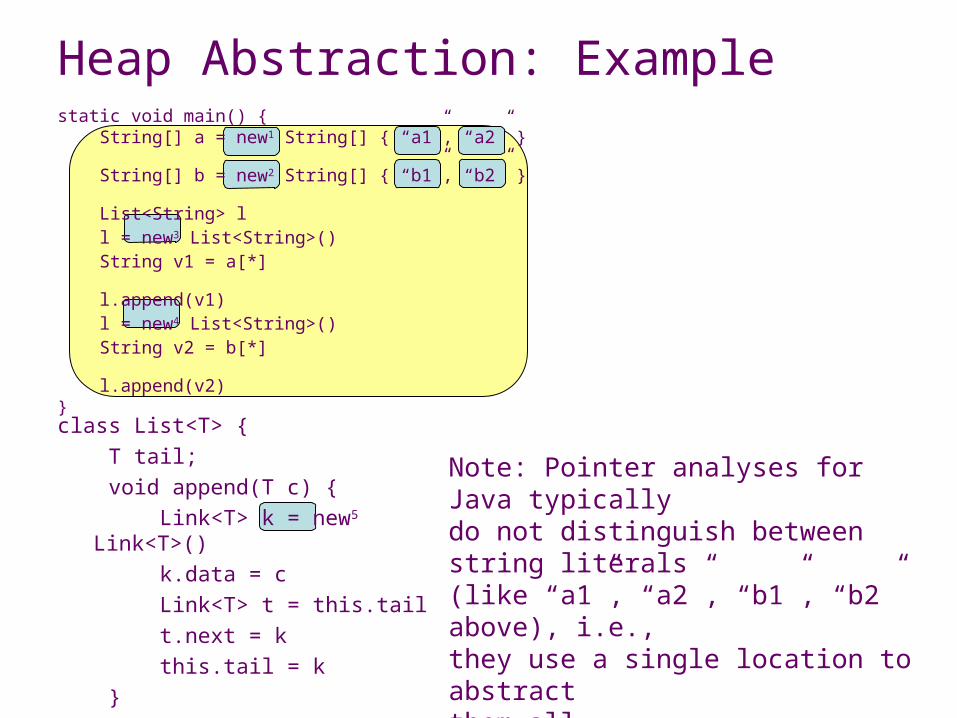
Heap Abstraction: Example
class List<T> { T tail; void append(T c) { Link<T> k = new5 Link<T>() k.data = c Link<T> t = this.tail t.next = k this.tail = k }}
Note: Pointer analyses for Java typicallydo not distinguish between string literals(like “a1”, “a2”, “b1”, “b2” above), i.e.,they use a single location to abstractthem all
static void main() { String[] a = new1 String[] { “a1”, “a2” }
String[] b = new2 String[] { “b1”, “b2” }
List<String> l
l = new3 List<String>() String v1 = a[*]
l.append(v1) l = new4 List<String>() String v2 = b[*]
l.append(v2)}
v = newi …
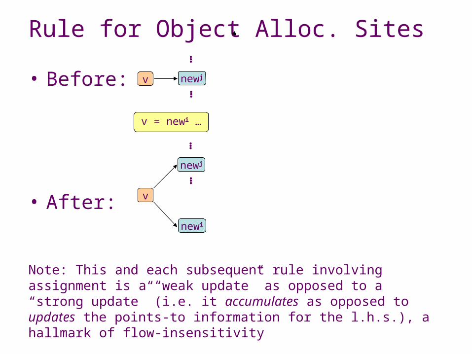
Rule for Object Alloc. Sites
• Before:
• After:
Note: This and each subsequent rule involving assignment is a “weak update” as opposed to a “strong update” (i.e. it accumulates as opposed to updates the points-to information for the l.h.s.), a hallmark of flow-insensitivity
v newj
……
v
newi
newj
……

Rule for Object Alloc. Sites: Examplestatic void main() { String[] a = new1 String[] { “a1”, “a2” }
String[] b = new2 String[] { “b1”, “b2” }
List<String> l
l = new3 List<String>() String v1 = a[*]
l.append(v1) l = new4 List<String>() String v2 = b[*]
l.append(v2)}class List<T> { T tail; void append(T c) { Link<T> k = new5 Link<T>() k.data = c Link<T> t = this.tail t.next = k this.tail = k }}
l
new4new3
new1
ba
new2

• Flow sensitivity– flow-insensitive: ignores intra-procedural control flow
• Heap abstraction– object allocation sites: does not distinguish between
objects allocated at same site
• Aggregate modeling– does not distinguish between elements of same array– field-sensitive for instance fields
• Context sensitivity
0-CFA Pointer Analysis for Java
v1.f = v2
v1
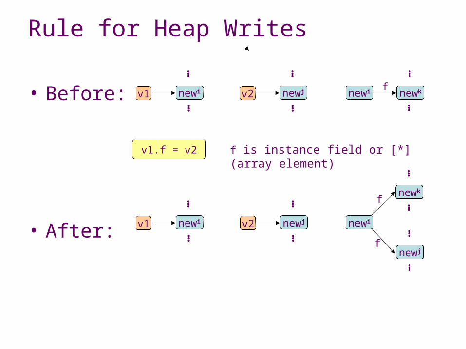
Rule for Heap Writes
• Before:
• After:
newi
……
v2 newj
……
v2 newj
……
newknewi
……
newi
f
newj
newk
……
……v1 newi
…… f
f
f is instance field or [*] (array element)

Rule for Heap Writes: Examplestatic void main() { String[] a = new1 String[] { “a1”, “a2” }
String[] b = new2 String[] { “b1”, “b2” }
List<String> l
l = new3 List<String>() String v1 = a[*]
l.append(v1) l = new4 List<String>() String v2 = b[*]
l.append(v2)}class List<T> { T tail; void append(T c) { Link<T> k = new5 Link<T>() k.data = c Link<T> t = this.tail t.next = k this.tail = k }}
l
new4new3
new1
ba
new2
[*]
[*]
“a1”
“a2”
[*]
[*]“b2”
“b1”

v1 = v2.f
v1
Rule for Heap Reads
• Before:
• After:
newi
v1
newk
newi
……
……
……
v2 newj
……
v2 newj
……
newknewj
……
f
newknewj
……
f
f is instance field or [*] (array element)
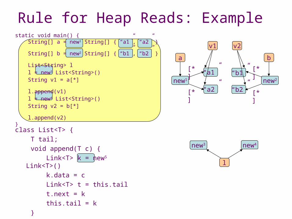
Rule for Heap Reads: Examplestatic void main() { String[] a = new1 String[] { “a1”, “a2” }
String[] b = new2 String[] { “b1”, “b2” }
List<String> l
l = new3 List<String>() String v1 = a[*]
l.append(v1) l = new4 List<String>() String v2 = b[*]
l.append(v2)}class List<T> { T tail; void append(T c) { Link<T> k = new5 Link<T>() k.data = c Link<T> t = this.tail t.next = k this.tail = k }}
l
new4new3
new1
ba
new2
[*]
[*]
“a1”
“a2”
[*]
[*]“b2”
“b1”
v1 v2

• Flow sensitivity– flow-insensitive: ignores intra-procedural control flow
• Heap abstraction– object allocation sites: does not distinguish between
objects allocated at same site
• Aggregate modeling– field-sensitive for instance fields– does not distinguish between elements of same array
• Context sensitivity– context-insensitive: ignores inter-procedural control
flow, analyzing each function in a single context
0-CFA Pointer Analysis for Java
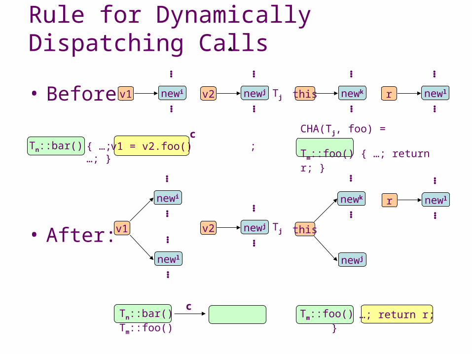
CHA(Tj, foo) =
Tm::foo() { …; return r; }v1 = v2.foo()
Rule for Dynamically Dispatching Calls
• Before:
• After: v1
newl
newi
v1 newi
……
……
……
v2 newj
……
v2 newj
……
this newk
……
r newl
……
Tj
Tj
r newl
……
this
newj
newk
……
{ …; ; …; }
Tn::bar() Tm::foo()
c
c
Tn::bar()
Tm::foo() { }…; return r;
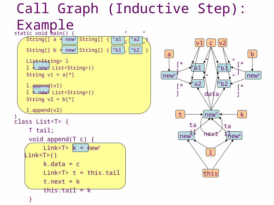
Call Graph (Inductive Step): Example
l
new4new3
new1
ba
new2
[*]
[*]
“a1”
“a2”
[*]
[*]“b2”
“b1”
v1 v2
static void main() { String[] a = new1 String[] { “a1”, “a2” }
String[] b = new2 String[] { “b1”, “b2” }
List<String> l
l = new3 List<String>() String v1 = a[*]
l.append(v1) l = new4 List<String>() String v2 = b[*]
l.append(v2)}class List<T> { T tail; void append(T c) { Link<T> k = new5 Link<T>() k.data = c Link<T> t = this.tail t.next = k this.tail = k }}
c
this
new5 k
data
tailtail
t
next

Classifying Pointer Analyses
• Heap abstraction
• Alias representation
• Aggregate modeling
• Flow sensitivity
• Context sensitivity
• Compositionality
• Adaptivity

Heap Abstraction
• Single node for entire heap– Cannot distinguish between heap-directed pointers – Popular in stack-directed pointer analyses for C
• Object allocation sites (“0-CFA”)– Cannot distinguish between objects allocated at same site– Predominant pointer analysis for Java
• String of call sites (“k-CFA with heap specialization/cloning”)– Distinguishes between objects allocated at same site using
finitely many strings of call sites– Predominant heap-directed pointer analysis for C
• Strings of object allocation sites in object-oriented languages(“k-object-sensitivity”)– Distinguishes between objects allocated at same site using
finitely many strings of object allocation sites

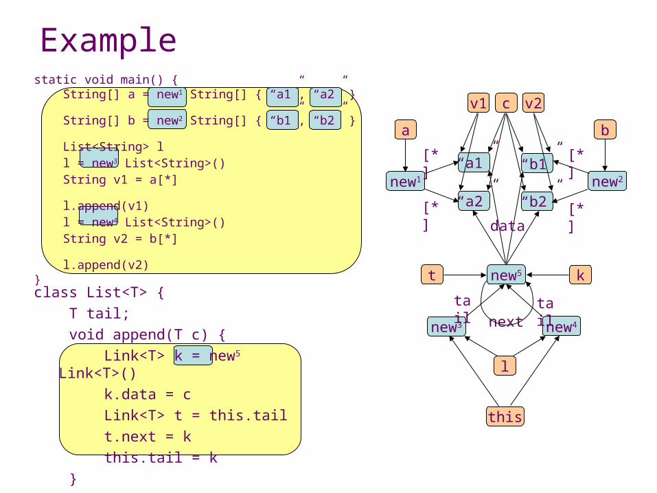
Example
l
new4new3
new1
ba
new2
[*]
[*]
“a1”
“a2”
[*]
[*]“b2”
“b1”
v1 v2
static void main() { String[] a = new1 String[] { “a1”, “a2” }
String[] b = new2 String[] { “b1”, “b2” }
List<String> l
l = new3 List<String>() String v1 = a[*]
l.append(v1) l = new4 List<String>() String v2 = b[*]
l.append(v2)}class List<T> { T tail; void append(T c) { Link<T> k = new5 Link<T>() k.data = c Link<T> t = this.tail t.next = k this.tail = k }}
c
this
new5 k
data
tailtail
t
next
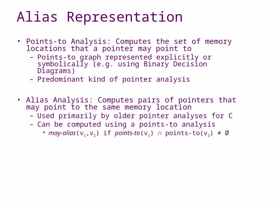
Alias Representation
• Points-to Analysis: Computes the set of memory locations that a pointer may point to– Points-to graph represented explicitly or symbolically (e.g.
using Binary Decision Diagrams)– Predominant kind of pointer analysis
• Alias Analysis: Computes pairs of pointers that may point to the same memory location– Used primarily by older pointer analyses for C– Can be computed using a points-to analysis
• may-alias(v1,v2) if points-to(v1) ∩ points-to(v2) ≠ Ø

Aggregate Modeling
• Arrays– Single field ([*]) representing all array elements– Cannot distinguish between elements of same array– Array dependence analysis used in parallelizing compilers
is capable of making such distinctions
• Records/Structs– Field-insensitive/field-independent: merge all fields of each
abstract record object– Field-based: merge each field of all record objects– Field-sensitive: model each field of each abstract record
object (most precise)

Flow Sensitivity
• Flow-insensitive– Ignores intra-procedural control-flow (i.e. order of
statements within a function)– Computes one solution for whole program or per function– Usually combined with Static Single Assignment (SSA)
transformation to get limited flow sensitivity– Two kinds:
• Steensgaard’s or equality-based: almost linear time• Anderson’s or subset-based: cubic time
• Flow-sensitive– Computes one solution per program point– More precise but less scalable

Example
l
new4new3
new1
ba
new2
[*]
[*]
“a1”
“a2”
[*]
[*]“b2”
“b1”
v1 v2
static void main() { String[] a = new1 String[] { “a1”, “a2” }
String[] b = new2 String[] { “b1”, “b2” }
List<String> l
l = new3 List<String>() String v1 = a[*]
l.append(v1) l = new4 List<String>() String v2 = b[*]
l.append(v2)}class List<T> { T tail; void append(T c) { Link<T> k = new5 Link<T>() k.data = c Link<T> t = this.tail t.next = k this.tail = k }}
c
this
new5 k
data
tailtail
t
next
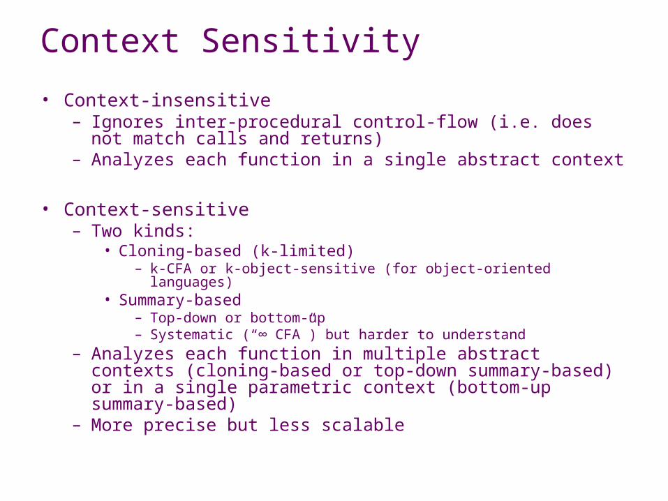
Context Sensitivity
• Context-insensitive– Ignores inter-procedural control-flow (i.e. does not match calls
and returns)– Analyzes each function in a single abstract context
• Context-sensitive– Two kinds:
• Cloning-based (k-limited)– k-CFA or k-object-sensitive (for object-oriented languages)
• Summary-based– Top-down or bottom-up– Systematic (“∞ CFA”) but harder to understand
– Analyzes each function in multiple abstract contexts (cloning-based or top-down summary-based) or in a single parametric context (bottom-up summary-based)
– More precise but less scalable
Example
l
new4new3
new1
ba
new2
[*]
[*]
“a1”
“a2”
[*]
[*]“b2”
“b1”
v1 v2
static void main() { String[] a = new1 String[] { “a1”, “a2” }
String[] b = new2 String[] { “b1”, “b2” }
List<String> l
l = new3 List<String>() String v1 = a[*]
l.append(v1) l = new4 List<String>() String v2 = b[*]
l.append(v2)}class List<T> { T tail; void append(T c) { Link<T> k = new5 Link<T>() k.data = c Link<T> t = this.tail t.next = k this.tail = k }}
c
this
new5 k
data
tailtail
t
next

Compositionality
• Whole-program– Cannot analyze open programs (e.g. libraries)– Predominant kind of pointer analysis
• Compositional/modular– Can analyze program fragments
• Missing callers (does not need “harness”)• Missing callees (does not need “stubs”)
– Solution is parameterized to accommodate unknown facts from the missing parts
– Solution is instantiated to yield less parameterized (or fully instantiated) solution when missing parts are encountered
– Parameterization harder in presence of dynamic dispatching• Existing approaches rely on call graph computed by a whole-
program analysis but can be highly imprecise– Open problem

Adaptivity
• Non-adaptive– Computes exhaustive solution of fixed precision regardless of
client
• Demand-driven– Computes partial solution, depending upon a query from a
client, but of fixed precision
• Client-driven– Computes exhaustive solution but can use different precision
in different parts of the solution, depending upon client
• Iterative/Refinement-based– Starts with an imprecise solution and refines it in successive
iterations depending upon client


![UCB CS294-88: Declarative Design [0.2cm] Chisel Overviewinst.eecs.berkeley.edu/~cs294-88/sp13/lectures/chisel-review.pdf · UCB CS294-88: Declarative Design Chisel Overview Jonathan](https://img.dokumen.tips/doc/110x75/60417694dde8db15be43b6a8/ucb-cs294-88-declarative-design-02cm-chisel-cs294-88sp13lectureschisel-reviewpdf.jpg)