POINT-LIKE BOUNDING CHAINS IN OPEN GROMOV-WITTENTHEORY

JAKE P. SOLOMON AND SARA B. TUKACHINSKY

Abstract. We use A∞ algebras to define open Gromov-Witten invariants with bothboundary and interior constraints, associated to a Lagrangian submanifold L ⊂ X ofarbitrary dimension. The boundary constraints are bounding chains, which are shown tobehave like points. The interior constraints are classes in the cohomology of X relative to L.We show the invariants satisfy analogs of the axioms of closed Gromov-Witten theory.

Our definition of invariants depends on the vanishing of a series of obstruction classes.One way to show vanishing is to impose certain cohomological conditions on L. Alternatively,if there exists an anti-symplectic involution fixing L, then part of the obstructions vanish apriori, and weaker cohomological conditions suffice to guarantee vanishing of the remainingobstructions. In particular, our definition generalizes both Welschinger’s and Georgieva’sreal enumerative invariants.

Contents

1. Introduction 21.1. Statement of results 21.2. Context 91.3. Outline 111.4. Acknowledgments 121.5. General notation 122. A∞ structures 122.1. Construction 122.2. Properties 142.3. Pseudoisotopies 163. Classification of bounding pairs 203.1. Additional notation 203.2. Existence of bounding chains 213.3. Gauge equivalence of bounding pairs 244. Real bounding pairs 284.1. Preliminaries 284.2. The real spin case 304.3. The case of Georgieva 355. Superpotential 365.1. Invariance under pseudoisotopy 365.2. Properties of bounding chains 375.3. Axioms of OGW 44

Date: Sep. 2019.2010 Mathematics Subject Classification. 53D45, 53D37 (Primary) 14N35, 14N10, 53D12 (Secondary).Key words and phrases. A∞ algebra, bounding chain, open Gromov-Witten invariant, Lagrangian submanifold,Gromov-Witten axiom, J-holomorphic, stable map, superpotential.

1

arX

iv:1

608.

0249

5v2

[m

ath.

SG]

5 S

ep 2

019

5.4. Relaxed relative de Rham complex 485.5. Comparison with Welschinger invariants 505.6. The case of Georgieva 50References 53

1. Introduction

Over a decade ago Welschinger [45–47] defined invariants that count real spheres withconjugation invariant configurations of point constraints in real symplectic manifolds ofcomplex dimensions 2 and 3. These invariants were subsequently related to counts ofJ-holomorphic disks with boundary and interior point constraints [37]. The problem ofextending the definition to higher dimensions has attracted much attention. Georgieva [18]solved the problem in odd dimensions in the absence of boundary constraints. We generalizeWelschinger’s invariants with both boundary and interior constraints to all dimensions usingthe language of A∞ algebras and bounding chains. Moreover, our definition does not requirea real structure.

1.1. Statement of results.

1.1.1. A∞ algebras. To formulate our results, we recall relevant notation from [39]. Consider asymplectic manifold (X,ω) of complex dimension n, and a connected, Lagrangian submanifoldL with relative spin structure s = sL. Let J be an ω-tame almost complex structure on X.Denote by µ : H2(X,L)→ Z the Maslov index. Denote by A∗(L) the ring of differential formson L with coefficients in R. Let Π = ΠL be the quotient of H2(X,L;Z) by a possibly trivialsubgroup SL contained in the kernel of the homomorphism ω ⊕ µ : H2(X,L;Z) → R ⊕ Z.Thus the homomorphisms ω, µ, descend to Π. Denote by β0 the zero element of Π. We usea Novikov ring Λ which is a completion of a subring of the group ring of Π. The precisedefinition follows. Denote by T β the element of the group ring corresponding to β ∈ Π, soT β1T β2 = T β1+β2 . Then,

Λ =

∞∑i=0

aiTβi

∣∣∣∣ai ∈ R, βi ∈ Π, ω(βi) ≥ 0, limi→∞

ω(βi) =∞

.

A grading on Λ is defined by declaring T β to be of degree µ(β). Denote also

Λ+ =

∞∑i=0

aiTβi ∈ Λ

∣∣∣∣ ω(βi) > 0 ∀i

.

We use a family of A∞ structures on A∗(L) ⊗ Λ following [12, 14], based on the resultsof [39]. Let Mk+1,l(β) be the moduli space of genus zero J-holomorphic open stable mapsu : (Σ, ∂Σ)→ (X,L) of degree [u∗([Σ, ∂Σ])] = β ∈ Π with one boundary component, k + 1boundary marked points, and l interior marked points. The boundary points are labeledaccording to their cyclic order. The space Mk+1,l(β) carries evaluation maps associated to

boundary marked points evbβj :Mk+1,l(β)→ L, j = 0, . . . , k, and evaluation maps associated

to interior marked points eviβj :Mk+1,l(β)→ X, j = 1, . . . , l.We assume that all J-holomorphic genus zero open stable maps with one boundary

component are regular, the moduli spaces Mk+1,l(β; J) are smooth orbifolds with corners,2

and the evaluation maps evbβ0 are proper submersions. Examples include (CP n,RP n) with thestandard symplectic and complex structures or, more generally, flag varieties, Grassmannians,and products thereof. See [39, Example 1.4, Remark 1.5]. Throughout the paper we fix aconnected component J of the space of ω-tame almost complex structures satisfying ourassumptions. All almost complex structures are taken from J . The results and arguments ofthe paper extend to general target manifolds with arbitrary ω-tame almost complex structuresif we use the virtual fundamental class techniques of [12,13,15–17]. Alternatively, it shouldbe possible to use the polyfold theory of [22–25,34]. The relative spin structure s determinesan orientation on the moduli spaces Mk+1,l(β) as in [14, Chapter 8].

Let s, t0, . . . , tN , be formal variables with deg s = 1− n. For m > 0 denote by Am(X,L)differential m-forms on X that vanish on L, and denote by A0(X,L) functions on X that areconstant on L. The exterior differential d makes A∗(X,L) into a complex. Alternatively, one

can consider the complex A∗(X,L) of forms on X with vanishing integral over L as explainedin Section 5.4. Set

R := Λ[[s, t0, . . . , tN ]], Q := R[t0, . . . , tN ],

C := A∗(L)⊗R, and D := A∗(X,L)⊗Q,

where ⊗ is understood as the completed tensor product. For an R-algebra Υ, write

H∗(X,L; Υ) := H∗(A∗(X,L)⊗Υ, d).

Observe that

H∗(X,L; Υ) '(H0(L;R)⊕H>0(X,L;R)

)⊗Υ, H∗(X,L;Q) = H∗(D).

The gradings on C,D, and H∗(X,L;Q), take into account the degrees of s, tj, Tβ, and the

degree of differential forms. Given a graded module M , we write Mj or (M)j for the degree jpart. Let

R+ := RΛ+ / R, IR := 〈s, t0, . . . , tN〉+R+ / R, IQ := 〈t0, . . . , tN〉 / Q,

be the ideals generated by the formal variables.Let γ ∈ IQD be a closed form with degD γ = 2. For example, given closed differential

forms γj ∈ A∗(X,L) for j = 0, . . . , N, take tj of degree 2− |γj| and γ :=∑N

j=0 tjγj. Definestructure maps

mγk : C⊗k −→ C

by

mγk(α1, . . . , αk) :=

= δk,1 · dα1 + (−1)∑kj=1 j(|αj |+1)+1

∑β∈Πl≥0

T β1

l!evbβ0 ∗(

l∧j=1

(eviβj )∗γ ∧k∧j=1

(evbβj )∗αj).

The push-forward (evbβ0 )∗ is defined by integration over the fiber; it is well-defined because

evbβ0 is a proper submersion. The condition γ ∈ IQD ensures that the infinite sum converges.Intuitively, γ should be thought of as interior constraints, while αj are boundary constraints.Then the output is a cochain on L that is “Poincare dual” to the image of the boundaries of

3

disks that satisfy the given constraints. In [39], as summarized in Proposition 2.1 below, weshow that (C, mγ

kk≥0) is an A∞ algebra. Furthermore, define

mγ−1 :=

∑β∈Πl≥0

1

l!T β∫M0,l(β)

l∧j=1

(eviβj )∗γ.

1.1.2. Bounding pairs and the superpotential. Our strategy is to extract OGW invariantsfrom the superpotential. For us, the superpotential is a function on the space of (weak)bounding pairs:

Definition 1.1. A bounding pair with respect to J is a pair (γ, b) where γ ∈ IQD is closedwith degD γ = 2 and b ∈ IRC with degC b = 1, such that∑

k≥0

mγk(b⊗k) = c · 1, c ∈ IR, degR c = 2. (1)

In this situation, following [14], b is called a bounding chain for mγ.

The standard superpotential is given by

Ω(γ, b) := ΩJ(γ, b) := (−1)n(∑k≥0

1

(k + 1)〈mγ

k(b⊗k), b〉+ mγ

−1

).

Intuitively, Ω counts J-holomorphic disks with constraints γ in the interior and b on the bound-ary. Modification is necessary in order to avoid J-holomorphic disks the boundary of whichcan degenerate to a point, forming a J-holomorphic sphere. We say that a monomial elementof R is of type D if it has the form a T βs0tj00 · · · t

jNN with a ∈ R and β ∈ Im(H2(X;Z)→ Π).

In the present paper, the superpotential is defined by

Ω(γ, b) := ΩJ(γ, b) := ΩJ(γ, b)− all monomials of type D in ΩJ .

Definition 3.10 gives a notion of gauge equivalence between a bounding pair (γ, b) with respectto J and a bounding pair (γ′, b′) with respect to another almost complex structure J ′. Let ∼denote the resulting equivalence relation.

Theorem 1 (Invariance of the super-potential). If (γ, b) ∼ (γ′, b′), then ΩJ(γ, b) = ΩJ ′(γ′, b′).

To obtain invariants from Ω, we must understand the space of gauge equivalence classes ofbounding pairs. Assume n > 0. Define a map

% : bounding pairs/ ∼ −→ (IQH∗(X,L;Q))2 ⊕ (IR)1−n

by

%([γ, b]) :=

([γ] ,

∫L

b

). (2)

We prove in Lemma 3.13 that % is well defined.

Theorem 2 (Classification of bounding pairs – rational cohomology spheres). AssumeH∗(L;R) = H∗(Sn;R). Then % is bijective.

4

Remark 1.2. Theorem 2 says that a bounding chain is determined up to equivalence by itspart that has degree n in A∗(L). In general, the degree n part of b must be “corrected” bynon-closed forms of lower degrees in order to solve equation (1). The degree n part is amultiple of a form that represents the Poincare dual of a point. In this sense the boundingchains of Theorem 2 are point-like.

In the presence of an anti-symplectic involution, the assumptions on L can be relaxed. Areal setting is a quadruple (X,L, ω, φ) where φ : X → X is an anti-symplectic involutionsuch that L ⊂ fix(φ). Throughout the paper, whenever we discuss a real setting, we fix aconnected subset Jφ ⊂ J consisting of J ∈ J such that φ∗J = −J. All almost complexstructures of a real setting are taken from Jφ. If we use virtual fundamental class techniques,we can treat any ω-tame almost complex structure J satisfying φ∗J = −J. Whenever wediscuss a real setting, we take SL ⊂ H2(X,L;Z) with Im(Id +φ∗) ⊂ SL, so φ∗ acts onΠL = H2(X,L;Z)/SL as − Id . Also, the formal variables ti have even degree. We denote

by Hevenφ (X,L;R) (resp. Heven

φ (X;R)) the direct sum over k of the (−1)k-eigenspace of φ∗

acting on H2k(X,L;R) (resp. H2k(X;R)). Note that the Poincare duals of φ-invariant almost

complex submanifolds of X disjoint from L belong to Hevenφ (X,L;R). Extend the action of

φ∗ to Λ, Q,R,C, and D, by taking

φ∗T β = (−1)µ(β)/2T β, φ∗ti = (−1)deg ti/2ti, φ∗s = −s. (3)

Elements a ∈ Λ, Q,R,C,D, and pairs thereof are called real if

φ∗a = −a. (4)

For a group Z on which φ∗ acts, let Z−φ∗ ⊂ Z denote the elements fixed by −φ∗. Let

%φ : real bounding pairs/ ∼ −→ (IQH∗(X,L;Q))−φ∗

2 ⊕ (IR)1−n

be given by the same formula as %. Then, we obtain the following variant of Theorem 2.

Theorem 3 (Classification of bounding pairs – real spin case). Suppose (X,L, ω, φ) is a realsetting, s is a spin structure, and n 6≡ 1 (mod 4). Moreover,

• if n ≡ 3 (mod 4), assume H i(L;R) ' H i(Sn;R) for i ≡ 0, 3 (mod 4);• if n ≡ 2 (mod 4), assume H i(L;R) ' H i(Sn;R) for i 6≡ 1 (mod 4);• if n ≡ 0 (mod 4), assume H i(L;R) ' H i(Sn;R) for i 6≡ 2 (mod 4).

Then %φ is bijective.

Remark 1.3. In the special cases when n = 2, 3, the cohomological assumption is alwayssatisfied. This explains the significance of dimensions 2 and 3 in Welschinger’s work [46,47].See Theorem 5 for a comparison of Welschinger’s invariants with the invariants of the presentwork.

Remark 1.4. In an earlier version of this paper in the case n ≡ 3 (mod 4), we used three-typical bounding chains instead of real bounding chains. Lemma 4.8 shows the two notionsare equivalent.

1.1.3. Open Gromov-Witten invariants and axioms. When the hypothesis of either Theorem 2or 3 is satisfied, we define open Gromov-Witten invariants as follows. In the case of Theorem 3,take SL containing Im(Id +φ∗). In the case of Theorem 2 (resp. Theorem 3) let WL =

5

H∗(X,L;R) (resp. WL = Hevenφ (X,L;R)). Fix Γ0, . . . ,ΓN , a basis of WL, set deg tj = 2−|Γj|,

and take

Γ :=N∑j=0

tjΓj ∈ (IQH∗(X,L;Q))2.

By Theorem 2 (resp. Theorem 3), choose (γ, b) such that

%([γ, b]) = (Γ, s) (resp. %φ([γ, b]) = (Γ, s)). (5)

By Theorem 1, the superpotential Ω = Ω(γ, b) is independent of the choice of (γ, b).

Definition 1.5. The open Gromov-Witten invariants of (X,L),

OGWβ,k = OGWLβ,k : W⊗l

L → R,are defined by setting

OGWβ,k(Γi1 , . . . ,Γil) := the coefficient of T β in ∂ti1 · · · ∂til∂ksΩ|s=0,tj=0

and extending linearly to general input.

It is not hard to see these invariants are independent of the choice of basis Γj. Also, it isnot hard to see that the invariants arising from Theorem 2 and Theorem 3 coincide whenboth hypotheses are satisfied. Write γ =

∑Nj=0 tjγj with γj ∈ A∗(X,L), so [γj] = Γj. The

invariant OGWβ,k(Γi1 , . . . ,Γil) counts configurations of disks that collectively have degreeβ, k boundary point-constraints, and interior constraints γi1 , . . . , γil . Figure 1 illustratesa configuration that may contribute to OGWβ,3(Γ1,Γ2,Γ3,Γ4,Γ5,Γ6). The notation bj, βj,comes from a decomposition b =

∑j T

βjbj with bj ∈ A∗(L)[[s, t0, . . . , tN ]]. The illustrationshows cycles that intuitively represent the “Poincare duals” of the non-closed differentialforms bj.

Remark 1.6. When n is even, it follows that deg s = 1− n is odd, so s2 = 0. Thus, for k > 1,we have OGWβ,k = 0. In work in progress, the definition of the invariants OGWβ,k for n evenis modified so that they take non-zero values for k > 1.

Theorem 4 (Axioms of the OGW invariants). The invariants OGW defined above have thefollowing properties. Let Aj ∈ WL for j = 1, . . . , l.

(1) (Degree) OGWβ,k(A1, . . . , Al) = 0 unless

n− 3 + µ(β) + k + 2l = kn+l∑

j=1

|Aj|. (6)

(2) (Symmetry) For any permutation σ ∈ Sl,

OGWβ,k(A1, . . . , Al) = (−1)sσ(A) OGWβ,k(Aσ(1) . . . , Aσ(l)), (7)

where sσ(A) :=∑

i>jσ(i)<σ(j)

degAσ(i) · degAσ(j).

(3) (Unit / Fundamental class)

OGWβ,k(1, A1, . . . , Al−1) =

−1, (β, k, l) = (β0, 1, 1),

0, otherwise.(8)

6

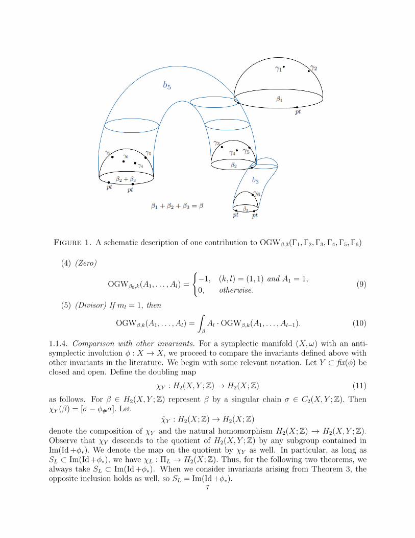
Figure 1. A schematic description of one contribution to OGWβ,3(Γ1,Γ2,Γ3,Γ4,Γ5,Γ6)

(4) (Zero)

OGWβ0,k(A1, . . . , Al) =

−1, (k, l) = (1, 1) and A1 = 1,

0, otherwise.(9)

(5) (Divisor) If ml = 1, then

OGWβ,k(A1, . . . , Al) =

∫β

Al ·OGWβ,k(A1, . . . , Al−1). (10)

1.1.4. Comparison with other invariants. For a symplectic manifold (X,ω) with an anti-symplectic involution φ : X → X, we proceed to compare the invariants defined above withother invariants in the literature. We begin with some relevant notation. Let Y ⊂ fix(φ) beclosed and open. Define the doubling map

χY : H2(X, Y ;Z)→ H2(X;Z) (11)

as follows. For β ∈ H2(X, Y ;Z) represent β by a singular chain σ ∈ C2(X, Y ;Z). ThenχY (β) = [σ − φ#σ]. Let

χY : H2(X;Z)→ H2(X;Z)

denote the composition of χY and the natural homomorphism H2(X;Z) → H2(X, Y ;Z).Observe that χY descends to the quotient of H2(X, Y ;Z) by any subgroup contained inIm(Id +φ∗). We denote the map on the quotient by χY as well. In particular, as long asSL ⊂ Im(Id +φ∗), we have χL : ΠL → H2(X;Z). Thus, for the following two theorems, wealways take SL ⊂ Im(Id +φ∗). When we consider invariants arising from Theorem 3, theopposite inclusion holds as well, so SL = Im(Id +φ∗).

7

The following theorem relates Welschinger’s invariants [46,47] to the invariants OGWβ,k

associated with a real setting (X,L, ω, φ). For d ∈ H2(X;Z), l ∈ Z≥0, write

kd,l =c1(X)(d)− 2(n− 1)l + n− 3

2.

For n = 2, 3, and either kd,l ≥ 1 or d /∈ Im χL, denote byWd,l Welschinger’s invariant countingreal rational J-holomorphic curves in (X,φ) of degree d with real locus in L passing throughkd,l real points and l pairs of φ-conjugate points. Although [47] does not allow the casekd,l = 0 and d /∈ Im χL, the definition extends without modification. Recall from Remark 1.3that when n = 2, 3, the hypothesis of Theorem 3 is always satisfied, so the invariants OGWβ,k

are defined.

Theorem 5 (Comparison with Welschinger’s invariants). Suppose n = 2 or 3. Let A ∈H2nφ (X,L;R) be the Poincare dual of a point. Let d ∈ H2(X;Z), l ∈ Z≥0, such that if n = 3,

then either kd,l ≥ 1 or d /∈ Im χL, and if n = 2, then kd,l = 1. Then,∑χL(β)=d

OGWβ, kd,l(A⊗l) = ±21−l · Wd, l.

Remark 1.7. When n = 2, the hypothesis kd,l = 1 is necessary. Indeed, by Remark 1.6, theopen Gromov-Witten invariants OGWβ,k vanish whenever k > 1, but it is shown in [29,30]that Welschinger’s invariants Wd,l do not generally vanish when kd,l > 1. On the other hand,the modified invariants mentioned in Remark 1.6 coincide with Welschinger’s invariants alsofor kd,l > 1 when n = 2.

The following theorem relates the invariants of Georgieva [18] for (X,ω, φ) to the invariantsOGWL

β,k : W⊗lL → R associated to the components L ⊂ fix(φ). The invariants OGWL

β,k

may arise from either Theorem 2 or Theorem 3 depending on which hypothesis is satisfiedby L. The group ΠL and the vector space WL are taken accordingly. Assume (X,ω, φ) isadmissible in the sense of [18], choose a φ-orienting structure as in [18], and let sL be theassociated relative spin structure for the component L ⊂ fix(φ). Recall that sL determinesa class wsL ∈ H2(X;Z/2Z) such that w2(TL) = i∗wsL . Let A ⊂ H2(X;Q) denote thecomplement of the image of χfix(φ) composed with the natural map H2(X;Z)→ H2(X;Q).

For d ∈ A and Aj ∈ H∗(X;R), let OGWGeorgievad,0,l (A1, . . . , Al) denote the invariant of [18].

Let Wφ denote H∗(X;R)−φ∗

if the hypothesis of Theorem 2 holds for each componentL ⊂ fix(φ). Otherwise, let Wφ denote Heven

φ (X;R)−φ∗

= ⊕m oddH2m(X;R)−φ

∗. The natural

map H∗(X,L;R)−φ∗ → H∗(X;R)−φ

∗is an isomorphism by the long exact sequence of the

pair (X,L). So, we identify Wφ with a subspace of WL for each component L ⊂ fix(φ).

Theorem 6 (Comparison with Georgieva’s invariants). Suppose (X,ω, φ) is admissible in thesense of [18], and the hypothesis of either Theorem 2 or Theorem 3 holds for each component

L ⊂ fix(φ). Assume that µ(β)2

+wsL(χL(β)) ≡ 0 (mod 2) for all components L ⊂ fix(φ) andall β ∈ ΠL. Then, for d ∈ A and Aj ∈ Wφ, we have∑

χL(β)=d,L⊂fix(φ)

OGWLβ,0(A1, . . . , Al) = 21−l OGWGeorgieva

d,0,l (A1, . . . , Al).

8

Remark 1.8. Theorem 6 does not generalize if we replace Wφ with H∗(X;R) or Hevenφ (X;R).

Indeed, the invariants OGWGeorgievad,0,l (A1, . . . , Al) are known to vanish if there is a j such that

φ∗Aj = Aj. However, the invariants OGWLβ,0 do not generally vanish as shown in [40].

Remark 1.9. On the other hand, when L satisfies the hypothesis of Theorem 3 but notof Theorem 2, the invariants OGWL

β,k(A1, . . . , Al) are defined only for A1, . . . , Al ⊂ H∗φ(X)

whereas the invariants OGWGeorgievaβ,0,l (A1, . . . , Al) are defined for A1, . . . , Al ∈ H∗(X). In

Section 5.6 we show how to use the superpotential to recover the invariants OGWGeorgievaβ,0,l

in this case as well using a classification result for a modified notion of real bounding pairsgiven in Section 4.3.

1.2. Context.

1.2.1. The symmetry approach. Several existing approaches utilize symmetries to define openinvariants in certain cases. Katz-Liu [32] and Liu [35] use an S1 action. Using anti-symplecticinvolutions, Cho [8] and Solomon [37], both in dimensions 2 and 3, define open invariantsthat generalize Welschinger’s real enumerative invariants [46,47]. Georgieva [18] uses anti-symplectic involutions to treat higher dimensions in the absence of boundary constraints. Asimilar result can be deduced from [37].

1.2.2. The superpotential. The problem of defining open Gromov-Witten invariants withoutusing symmetries has a long history. The idea of using the superpotential to define holomorphicdisk counting invariants goes back to [50]. Subsequently, the superpotential has been discussedwidely in the physics literature [21, 33, 42–44]. It is explained in [36, Section 0.4] that theinvariants of [37] in the Calabi-Yau setting can be extracted from a critical value of thesuperpotential. The use of bounding chains along with the superpotential to define invariantswas suggested by Joyce [31, Section 6.2].

1.2.3. Vanishing Maslov class. Fukaya [13] uses the superpotential and bounding chainsto define open Gromov-Witten invariants for a Lagrangian submanifold L with vanishingMaslov class in a Calabi-Yau threefold. In the Maslov zero setting, the grading on Λ is trivial.Moreover, when dimL = 3, Maslov zero disks have expected dimension zero. So, boundary andinterior constraints as well as the corresponding variables ti and s are irrelevant. Consequently,it is natural to take R = Λ and the degree 1 elements of C are necessarily 1-forms. Also,bounding chains are necessarily strong, that is, the constant c of equation (1) vanishes. Strongbounding chains are critical points of the superpotential. So, the superpotential is constanton each connected component (in an appropriate non-Archimedean sense) of the space ofbounding chains. Thus, if one can identify a connected component of the space of boundingchains, evaluating the superpotential at any point therein will give the same invariant. Infavorable situations, there may be only one connected component.

There are several other works in the Maslov zero setting, which should be related to that ofFukaya [13]. Aganagic-Ekholm-Ng-Vafa [2] define open Gromov-Witten invariants for knots,and Ekholm-Shende [10] construct open Gromov-Witten invariants valued in skeins. Cho [9]defines an invariant function similar to the superpotential on Hochschild cycles. Iacovinodefines a superpotential counting “multi-curves” in Calabi-Yau threefolds [26,27]. He thenrephrases his construction in the language of obstruction theory [28].

9

1.2.4. Non-vanishing Maslov class. When the Maslov class of the Lagrangian submanifoldL ⊂ X does not vanish, strong bounding chains generally do not exist. Rather, one mustconsider weak bounding chains [14] as we do in the present article. Weak bounding chainsare not critical points of the superpotential. So, the value of the superpotential depends onthe precise choice of bounding chain, as opposed to its connected component in the Maslovzero case. On the other hand, the fact that weak bounding chains are not critical pointsmeans that the superpotential can give rise to larger families of invariants. Indeed, if onecan find a canonically parameterized family of bounding chains on which to evaluate thesuperpotential, one obtains a parameterized family of invariants. The parameter k in theinvariants OGWβ,k(·) of the present work arises in this way from the s dependence of b.

Fukaya-Oh-Ohta-Ono [17] study a potential function on the space of weak boundingchains, which is essentially the derivative of the superpotential discussed here, in the contextof Lagrangian tori in compact toric manifolds. They recover quantum cohomology, orequivalently, closed Gromov-Witten theory, as the Jacobian ring of the potential. However,there does not seem to be a canonical parameterization of the space of weak bounding chainsin that context, so it is not clear how to extract a numerical invariant by evaluating thesuperpotential on a bounding chain. Nonetheless, Fukaya [13, Section 8.3] thinks it likelythe superpotential approach can be used to recover the invariants of [37, 46, 47]. The presentpaper confirms the superpotential approach does in fact recover these invariants and moreover,extends them to arbitrary odd dimension.

1.2.5. The present work. Theorems 2 and 3 allow us to choose canonical bounding chainson which the superpotential can be evaluated to obtain invariants. Theorems 5 and 6 showthe invariants obtained from the superpotential recover the invariants of Welschinger [46, 47]and Georgieva [18]. In particular, Theorem 5 shows that bounding chains play the role ofboundary point constraints, Poincare dual to n-forms, contrary to the intuition from theCalabi-Yau case where bounding chains are 1-forms.

The proof of Theorem 3 clarifies the importance of anti-symplectic involution symmetryin defining invariants. Namely, such an involution forces part of the obstructions to theexistence and uniqueness of bounding chains to vanish. The fact that not all obstructions areforced to vanish explains why the symmetry approach only works in low dimensions [46,47]or in the absence of boundary constraints [18]. The cohomological hypothesis of Theorem 3is used to deal with the obstructions that are not forced to vanish by symmetry.

The present work explains why boundary constraints in the open Gromov-Witten invariantsof [8,37,46,47] could only be points and not arbitrary cycles. Indeed, to construct a canonicalfamily of bounding chains, we use the map % (2), which integrates bounding chains over L.The proof in Lemma 3.13 that % is invariant under gauge equivalence makes crucial use ofthe top degree property of A∞ pseudoisotopies, Proposition 2.19. In particular, integratingover any cycle on L apart from the fundamental class would not give a well-defined map.As explained in Remark 1.2, it follows from the definition of % that our canonical family ofbounding chains is point-like. Even if we suppose there exists a canonical family of boundingchains involving more parameters than %, it is shown in Remark 4.16 of [40] that genericallythe superpotential only depends on the parameters of %.

Theorem 4 shows that the superpotential invariants, despite their abstract definition, satisfysimple axioms analogous to those of closed Gromov-Witten theory. To prove Theorem 4,Definition 5.1 formulates properties of bounding chains analogous to the fundamental class

10

and divisor axioms. Under the assumptions of Theorem 2 (resp. Theorem 3), Proposition 5.2(resp. Proposition 5.3) shows that any gauge equivalence class of bounding chains has arepresentative that satisfies these axioms.

It is known [5–7] that Welschinger’s invariants for (CP 3,RP 3), and thus also the invariantsOGWβ,k(·) of the present paper, are non-zero for many choices of β, interior constraints,and both k = 0 and k > 0. It is known [11, 19] that Georgieva’s invariants and thus alsoOGWβ,0(·) are non-zero for (CP n,RP n) with n > 3 odd and various choices of β and interiorconstraints. In [40], we give recursive formulas that completely determine the invariantsOGWβ,k(·) in the case (X,L) = (CP n,RP n) with n odd. In particular, these invariants areshown to be non-zero for many choices of β and interior constraints even when both n > 3and k > 0. Furthermore, the invariants OGWβ,0(A1, . . . , Al) are shown to be non-zero inmany cases even when φ∗Aj = Aj for one or more j, whereas the invariants of Georgieva [18]vanish.

1.2.6. Future plans. Work in progress proves an analogue of Theorem 2 under the weakercohomological assumption that the restriction map Hm(X;R)→ Hm(L;R) is surjective for0 < m < n. As mentioned in Remark 1.6, work in progress modifies the definition of theinvariants OGWβ,k in even dimensions so they no longer vanish when k > 1. Theorem 5extends accordingly as mentioned in Remark 1.7. Another work in progress extends thedefinition of the invariants so that L need not be orientable. Furthermore, we plan to applythe techniques of the present paper to the non-compact Calabi-Yau setting studied in [20]and [1].

1.2.7. Related work. Welschinger [48,49] corrects disk bubbling by taking into account linkingnumbers, thus obtaining invariants in dimensions 2 and 3. We expect this approach is closelyrelated to the present paper. Another related approach is being developed by Tessler [41].

Netser Zernik [51, 52] follows an approach closely related to the present work to defineequivariant open Gromov-Witten invariants and give an equivariant localization formula forthem.

Biran-Cornea [3] define an invariant of Lagrangian 2-tori counting disks of a given degreethrough three points. The invariant arises as the discriminant of a quadratic form associatedto the Lagrangian quantum product. Biran-Membrez [4] define a related invariant for evendimensional Lagrangian spheres. Cho [9] gives an example of an open Gromov-Witteninvariant for the Clifford torus in CP 2. It would be interesting to find a connection betweenany of these invariants and those of the present paper.

1.3. Outline. In Section 2 we quote some results from [39] that will be useful in the othersections. This includes the construction of the A∞ structure in Section 2.1 using q operators,properties of the q operators in Section 2.2, and the notion of pseudoisotopies between twoA∞ structures in Section 2.3.

Section 3 contains results concerning bounding pairs, most notably a construction ofbounding pairs in Section 3.2 and a construction of gauge equivalences of bounding pairsin Section 3.3. Together, these two sections prove Theorem 2, as detailed in the end ofSection 3.3.

Section 4 deals with the real setting. After establishing signs of conjugation in Section 4.1,we move to proving Theorem 3 in Section 4.2. Section 4.3 proves a classification result for a

11

modified notion of real bounding pairs, which leads to an interpretation of the invariants ofGeorgieva [18] in terms of the superpotential.

Section 5 concerns the superpotential and the open Gromov-Witten invariants OGWβ,k

derived from it. In Section 5.1 we show the superpotential is invariant under pseudoisotopyproving Theorem 1. In Section 5.2 we construct bounding chains with properties reminiscentof the Gromov-Witten axioms. Section 5.3 proves the axioms of the open Gromov-Witteninvariants OGWβ,k, that is, Theorem 4. Section 5.4 shows how to adapt the proofs of

Theorems 1-4 to the complex A∗(X,L) in place of A∗(X,L). The complex A∗(X,L) plays animportant role in [40]. Section 5.5 compares the invariants OGWβ,k with those of Welschingerproving Theorem 5. Section 5.6 applies the superpotential to the modified real boundingpairs of Section 4.3 to obtain open Gromov-Witten invariants under assumptions similar tothose of Georgieva [18]. These invariants are related to both Georgieva’s invariants and theinvariants OGWβ,k. The proof of Theorem 6 follows.

1.4. Acknowledgments. The authors would like to thank M. Abouzaid, D. Auroux, P. Ge-orgieva, D. Joyce, T. Kimura, E. Kosloff, M. Liu, L. Polterovich, E. Shustin, I. Smith, G. Tian,and A. Netser Zernik, for helpful conversations. The authors were partially supported byERC starting grant 337560 and ISF Grant 1747/13. The first author was partially supportedby ISF Grant 569/18. The second author was partially supported by the Canada ResearchChairs Program and NSF grant No. DMS-163852.

1.5. General notation.We write I := [0, 1] for the closed unit interval.Use i to denote the inclusion i : L → X. By abuse of notation, we also use i for

Id×i : I × L→ I ×X. The meaning in each case should be clear from the context.Denote by pt the map (from any space) to a point.Whenever a tensor product is written, we mean the completed tensor product.Write A∗(L;R) for A∗(L)⊗R. Similarly, A∗(X;R) and A∗(X,L;R) stand for A∗(X)⊗R

and A∗(X,L)⊗R, respectively.Given α, a homogeneous differential form with coefficients in R, denote by |α| the degree

of the differential form, ignoring the grading of R.For a possibly non-homogeneous α, denote by (α)j the form that is the part of degree j in

α. In particular, |(α)j| = j. Contrariwise, for a graded module M , the notation Mj or (M)jstands for the degree j part of the module, which in the present context involves degrees offorms as well as degrees of variables.

Let Υ′ be an R-vector space, Υ′′ = R, Q, or Λ, and let Υ = Υ′ ⊗ Υ′′. For x ∈ Υ andλ ∈ Υ′′, denote by [λ](x) ∈ Υ′ the coefficient of λ in x.

2. A∞ structures

In this section we recall definitions and results from [39]. The notation, as well as sign andorientation conventions, are the same as in [39], except that we have added the variable s toR (but not to Q).

2.1. Construction. Throughout this work (X,ω) is a symplectic manifold, L ⊂ X is aconnected Lagrangian submanifold with relative spin structure s, and J is an ω-tame almostcomplex structure. Let dimRX = 2n. Write β0 := 0 ∈ Π.

12

A J-holomorphic genus-0 open stable map to (X,L) of degree β ∈ Π with one boundarycomponent, k + 1 boundary marked points, and l interior marked points, is a quadruple(Σ, u, ~z, ~w) as follows. The domain Σ is a genus-0 nodal Riemann surface with boundaryconsisting of one connected component. The map

u : (Σ, ∂Σ)→ (X,L)

is continuous, J-holomorphic on each irreducible component of Σ, and [u∗([Σ, ∂Σ])] = β. Themarked points are denoted by

~z = (z0, . . . , zk), ~w = (w1, . . . , wl),

with zj ∈ ∂Σ, wj ∈ int(Σ), distinct. The labeling of the marked points zj respects the cyclicorder given by the orientation of ∂Σ induced by the complex orientation of Σ. Stability meansthat if Σi is an irreducible component of Σ, then either u|Σi is non-constant, or the combinednumber of marked points and nodal points on Σi is at least 3. An isomorphism of open stablemaps (Σ, u, ~z, ~w) and (Σ′, u′, ~z′, ~w′) is a homeomorphism θ : Σ→ Σ′, biholomorphic on eachirreducible component, such that

u = u′ θ, z′j = θ(zj), j = 0, . . . , k, w′j = θ(wj), j = 1, . . . , l.

Let Mk+1,l(β) =Mk+1,l(β; J) denote the moduli space of J-holomorphic genus zero openstable maps to (X,L) of degree β with one boundary component, k + 1 boundary markedpoints, and l internal marked points. Let the evaluation maps

evbβj :Mk+1,l(β)→ L, j = 0, . . . , k,

eviβj :Mk+1,l(β)→ X, j = 1, . . . , l,

be given by evbβj ((Σ, u, ~z, ~w)) = u(zj) and eviβj ((Σ, u, ~z, ~w)) = u(wj). We may omit thesuperscript β when the omission does not create ambiguity.

We assume that Mk+1,l(β) is a smooth orbifold with corners and that evbβ0 is a propersubmersion. The results and arguments of the paper extend to general target manifolds witharbitrary ω-tame almost complex structures if we use the virtual fundamental class techniquesof [12, 13, 15–17]. Alternatively, it should be possible to use the polyfold theory of [22–25,34].The relative spin structure s determines an orientation on Mk+1,l(β) as in [14, Chapter 8].

For all β ∈ Π, k, l ≥ 0, (k, l, β) 6∈ (1, 0, β0), (0, 0, β0), define

qβk, l : C⊗k ⊗ A∗(X;Q)⊗l −→ C

by

qβk,l(α1 ⊗ · · · ⊗ αk; γ1 ⊗ · · · ⊗ γl) := (−1)ε(α)(evbβ0 )∗

(l∧

j=1

(eviβj )∗γj ∧k∧j=1

(evbβj )∗αj

)with

ε(α) :=k∑j=1

j(degαj + 1) + 1.

The push-forward (evb0)∗ is defined by integration over the fiber; it is well-defined because

evb0 is a proper submersion. The case qβ0,0 is understood as −(evbβ0 )∗1. Define also qβ00,0 := 013

and qβ01,0(α) := dα. Set

q k, l :=∑β∈Π

T βqβk, l.

Furthermore, for l ≥ 0, (l, β) 6= (1, β0), (0, β0), define

qβ−1,l : A∗(X;Q)⊗l −→ Q

by

qβ−1,l(γ1 ⊗ · · · ⊗ γl) :=

∫M0,l(β)

l∧j=1

(eviβj )∗γj,

define qβ0−1,1 := 0, qβ0−1,0 := 0, and set

q−1,l(γ1 ⊗ · · · ⊗ γl) :=∑β∈Π

T βqβ−1,l(γ1 ⊗ · · · ⊗ γl).

Lastly, define similar operations using spheres,

q∅,l : A∗(X;Q)⊗l −→ A∗(X;Q),

as follows. For β ∈ H2(X;Z) let Ml+1(β) be the moduli space of genus zero J-holomorphicstable maps with l + 1 marked points indexed from 0 to l, representing the class β. Denoteby evβj :Ml+1(β)→ X the evaluation map at the j-th marked point. Assume that all the

moduli spacesMl+1(β) are smooth orbifolds and evβ0 is a submersion. Let $ : H2(X;Z)→ Πdenote the projection. For l ≥ 0, (l, β) 6= (1, 0), (0, 0), set

qβ∅,l(γ1, . . . , γl) := (evβ0 )∗(∧lj=1(evβj )∗γj), q0∅,1 := 0, q0

∅,0 := 0,

q∅,l(γ1, . . . , γl) :=∑

β∈H2(X)

T$(β)qβ∅,l(γ1, . . . , γl).

Fix a closed form γ ∈ IQD with degD γ = 2. Define maps on C by

mβ,γk (⊗kj=1αj) =

∑l

1

l!T βqβk, l(⊗

kj=1αj; γ

⊗l), mγk(⊗

kj=1αj) =

∑l

1

l!q k, l(⊗kj=1αj; γ

⊗l),

for all k ≥ −1, l ≥ 0. In particular, note that mγ−1 ∈ R.

Proposition 2.1 (A∞ relations [39, Proposition 2.7]). The operations mγkk≥0 define an

A∞ structure on C. That is,∑k1+k2=k+1

1≤i≤k1

(−1)∑i−1j=1(degαj+1)mγ

k1(α1, . . . , αi−1,m

γk2

(αi, . . . , αi+k2−1), αi+k2 , . . . , αk) = 0.

2.2. Properties. Denote by 〈 , 〉 the signed Poincare pairing

〈ξ, η〉 := (−1)deg η

∫L

ξ ∧ η. (12)

14

Proposition 2.2 (Linearity [39, Proposition 3.1]). The q operators are multilinear in thesense that for a ∈ R we have

qβk,l(α1, . . . , αi−1, a · αi, . . . , αk; γ1, . . . , γl) =

= (−1)deg a·(i+

∑i−1j=1 degαj+

∑lj=1 deg γj

)a · qβk,l(α1, . . . , αk; γ1, . . . , γl),

and for a ∈ Q we have

qβk,l(α1, . . . , αk; γ1, . . . , a · γi, . . . , γl) = (−1)deg a·∑i−1j=1 deg γja · qβk,l(α1, . . . , αk; γ1, . . . , γl),

andqβ∅,l(γ1, . . . , a · γi, . . . , γl) = (−1)deg a·

∑i−1j=1 deg γja · qβ∅,l(γ1, . . . , γl).

In addition, the pairing 〈 , 〉 defined by (12) is R-bilinear in the sense that

〈a.α1, α2〉 = a〈α1, α2〉, 〈α1, a.α2〉 = (−1)deg a·(1+degα1)a〈α1, α2〉.

Proposition 2.3 (Unit of the algebra [39, Proposition 3.2]). Fix f ∈ A0(L)⊗R, α1, . . . , αk ∈C, and γ1, . . . , γl ∈ A∗(X;Q). Then

qβk+1,l(α1, . . . , αi−1, f, αi, . . . , αk;⊗lr=1γr) =

=

df, (k + 1, l, β) = (1, 0, β0),

(−1)deg ff · α1, (k + 1, l, β) = (2, 0, β0), i = 1,

(−1)degα1(deg f+1)f · α1, (k + 1, l, β) = (2, 0, β0), i = 2,

0, otherwise.

In particular, 1 ∈ A0(L) is a strong unit for the A∞ operations mγ :

mγk+1(α1, . . . , αi−1, 1, αi, . . . , αk) =

0, k ≥ 2 or k = 0,

α1, k = 1, i = 1,

(−1)degα1α1, k = 1, i = 2.

Proposition 2.4 (Cyclic structure [39, Proposition 3.3]). For any α1, . . . , αk+1 ∈ C andγ1, . . . , γl ∈ A∗(X;Q),

〈q k, l(α1, . . ., αk; γ1, . . . γl), αk+1〉 =

(−1)(degαk+1+1)∑kj=1(degαj+1) · 〈q k, l(αk+1, α1, . . . , αk−1; γ1, . . . , γl), αk〉.

In particular, (C, mγkk≥0) is a cyclic A∞ algebra for any γ.

Proposition 2.5 (Degree of structure maps [39, Proposition 3.5]). For γ1, . . . , γl ∈ D2,k ≥ 0, the map

q k, l( ; γ1, . . . , γl) : C⊗k −→ C

is of degree 2− k.

Proposition 2.6 (Symmetry [39, Proposition 3.6]). Let k ≥ −1. For any permutationσ ∈ Sl,

q k, l(α1, . . . , αk; γ1, . . . , γl) = (−1)sσ(γ)q k, l(α1, . . . , αk; γσ(1), . . . , γσ(l)),

where sσ(γ) :=∑

i>jσ(i)<σ(j)

deg γσ(i) · deg γσ(j) (mod 2).

15

Proposition 2.7 (Fundamental class [39, Proposition 3.7]). For k ≥ 0,

qβk, l(α1, . . . , αk; 1, γ1, . . . , γl−1) =

−1, (k, l, β) = (0, 1, β0),

0, otherwise.

Furthermore,qβ−1,l(1, γ1, . . . , γl−1) = 0.

Proposition 2.8 (Energy zero [39, Proposition 3.8]). For k ≥ 0,

qβ0k, l(α1, . . . , αk; γ1, . . . , γl) =

dα1, (k, l) = (1, 0),

(−1)degα1α1 ∧ α2, (k, l) = (2, 0),

−γ1|L, (k, l) = (0, 1),

0, otherwise.

Furthermore,qβ0−1,l(γ1, . . . , γl) = 0.

Proposition 2.9 (Divisors [39, Proposition 3.9]). Assume γ1 ∈ A2(X,L)⊗Q, dγ1 = 0, andthe map H2(X,L;Z)→ Q given by β 7→

∫βγ1 descends to Π. Then

qβk, l(⊗kj=1αj;⊗lj=1γj) =

(∫β

γ1

)· qβk,l−1(⊗kj=1αj;⊗lj=2γj)

for k ≥ −1.

Proposition 2.10 (Top degree [39, Proposition 3.12]). Suppose

(k, l, β) 6∈ (1, 0, β0), (0, 1, β0), (2, 0, β0).Then (qβk, l(α; γ))n = 0 for all lists α, γ.

Remark 2.11. Proposition 2.2 shows the operations mγ are multilinear. Proposition 2.4 showsthe A∞ algebra (C,mγ) is cyclic. Proposition 2.3 shows unitality of (C,mγ) in the usualsense, and Proposition 2.10 shows an analog of unitality for mγ

0 . Thus, (C,mγ, 〈 , 〉, 1) is acyclic unital A∞ algebra in the sense of [39, Definition 1.1].

2.3. Pseudoisotopies. Set

C := A∗(I × L;R), D := A∗(I ×X, I × L;Q), R := A∗(I;R). (13)

We construct a family of A∞ structures on C. Let Jtt∈I be a path in J from J = J0 toJ ′ = J1. For each β, k, l, set

Mk+1,l(β) := (t, u, ~z, ~w) | (u, ~z, ~w) ∈Mk+1,l(β; Jt).We have evaluation maps

evbj : Mk+1,l(β) −→ I × L, j ∈ 0, . . . , k,

evbj(t, u, ~z, ~w) := (t, u(zj)),

and

evij : Mk+1,l(β) −→ I ×X, j ∈ 1, . . . , l

evij(t, u, ~z, ~w) := (t, u(wj)).

16

It follows from the assumption on J that all Mk+1,l(β) are smooth orbifolds with corners,

and evb0 is a proper submersion.

Example 2.12. In the special case when Jt = J = J ′ for all t ∈ I, we have Mk+1,l(β) =

I ×Mk+1,l(β; J). The evaluation maps in this case are evbj = Id×evbj and evij = Id×evij.

Let

p : I × L −→ I, pM : Mk+1,l(β) −→ I

denote the projections.Define

qβk,l : C⊗k ⊗ A∗(I ×X;Q)⊗l −→ C, k, l ≥ 0,

by

qβ0=01,0 (α) = dα, qβk,l(⊗

kj=1αj;⊗lj=1γj) := (−1)ε(α)(evb0)∗(∧lj=1evi

∗j γj ∧ ∧kj=1evb

∗j αj),

α, αj ∈ A∗(I × L), γj ∈ A∗(I ×X).

Define

qβ−1,l : A∗(I ×X;Q)l −→ A∗(I;Q), l ≥ 0,

by

qβ−1,l(⊗lj=1γj) := (pM)∗ ∧lj=1 evi

∗j γj.

As before, denote the sum over β by

qk,l(⊗kj=1αj;⊗lj=1γj) :=∑β∈Π

T β qβk,l(⊗kj=1αj;⊗lj=1γj),

q−1,l(⊗lj=1γj) :=∑β∈Π

T β q−1,l(γl).

Lastly, define similar operations using spheres,

q∅,l : A∗(I ×X;Q)⊗l −→ A∗(I ×X;R),

as follows. For β ∈ H2(X;Z) let

Ml+1(β) := (t, u, ~w) | (u, ~w) ∈Ml+1(β; Jt).For j = 0, . . . , l, let

evβj : Ml+1(β)→ I ×X,evβj (t, u, ~w) := (t, u(wj)),

be the evaluation maps. Assume that all the moduli spaces Ml+1(β) are smooth orbifoldsand ev0 is a submersion. For l ≥ 0, (l, β) 6= (1, 0), (0, 0), set

qβ∅,l(γ1, . . . , γl) := (evβ0 )∗(∧lj=1(evβj )∗γj),

and define q0∅,1 := 0, q0

∅,0 := 0, and

q∅,l(γ1, . . . , γl) :=∑

β∈H2(X)

T$(β)qβ∅,l(γ1, . . . , γl).

17

Write also

GW :=∑l≥0

1

l!p∗i∗q∅,l(γ).

Define a pairing on C:

〈〈 , 〉〉 : C⊗ C −→ R, 〈〈ξ, η〉〉 := (−1)deg ηp∗(ξ ∧ η).

Note that

〈〈ξ, η〉〉 = (−1)deg ηp∗(ξ∧η) = (−1)deg η+deg η·deg ξp∗(η∧ξ) = (−1)(deg η+1)(deg ξ+1)+1〈〈η, ξ〉〉. (14)

For each closed γ ∈ IQD with degD γ = 2, define structure maps

mγk : C⊗k −→ C

by

mγk(⊗

kj=1αj) :=

∑l

1

l!qk,l(⊗kj=1αj; γ

⊗l),

and define

mγ−1 :=

∑l

1

l!q−1,l(γ

⊗l) ∈ A∗(I;R).

Proposition 2.13 (A∞ structure [39, Proposition 4.5]). The maps mγ define an A∞ structureon C. That is,∑

k1+k2=k+1k1,k2≥0

(−1)∑i−1j=1(deg αj+1)mγ

k1(α1, . . . , αi−1, m

γk2

(αi, . . . , αi+k2−1), αi+k2 , . . . , αk) = 0

for all αj ∈ C.

Proposition 2.14 (Linearity [39, Proposition 4.6]). The operations q are R-multilinear inthe sense that for f ∈ R,

qβk,l(α1, . . . , αi−1, f.αi, . . . , αk; γ1, . . . , γl) =

= (−1)deg f ·(i+

∑i−1j=1 deg αj+

∑lj=1 deg γj

)f.qβk,l(α1, . . . , αk; γ1, . . . , γl) + δ1,k · df.α1,

and for f ∈ A∗(I;Q),

qβk,l(α1, . . . , αk; γ1, . . . , f.γi, . . . , γl) = (−1)deg f ·∑i−1j=1 deg γjf.qβk,l(α1, . . . , αk; γ1, . . . , γl),

and

qβ∅,l(γ1, . . . , f.γi, . . . , γl) = (−1)deg f ·∑i−1j=1 deg γjf.qβ∅,l(γ1, . . . , γl).

In addition, the pairing 〈〈 , 〉〉 is R-bilinear in the sense that

〈〈f.α1, α2〉〉 = f〈〈α1, α2〉〉, 〈〈α1, f.α2〉〉 = (−1)deg f ·(1+deg α1)f〈〈α1, α2〉〉.18

Proposition 2.15 (Unit of the algebra [39, Proposition 4.10]). Fix f ∈ A0(I × L) ⊗ R,α1, . . . , αk ∈ C, and γ1, . . . , γl ∈ A∗(I ×X;Q). Then

qβk+1,l(α1, . . . , αi−1, f, αi, . . . , αk;⊗lr=1γr) =

=

df, (k + 1, l, β) = (1, 0, β0),

(−1)deg f · α2, (k + 1, l, β) = (2, 0, β0), i = 1,

(−1)deg α1(deg f+1)f · α1, (k + 1, l, β) = (2, 0, β0), i = 2,

0, otherwise.

In particular, 1 ∈ A0(I × L) is a strong unit for the A∞ operations mγ:

mγk+1(α1, . . . , αi−1, 1, αi, . . . , αk) =

0, k + 1 ≥ 3 or k + 1 = 1,

α1, k + 1 = 2, i = 1,

(−1)deg α1α1, k + 1 = 2, i = 2.

Proposition 2.16 (Cyclic structure [39, Proposition 4.11]). The q are cyclic with respect tothe inner product 〈〈 , 〉〉. That is,

〈〈qk,l(α1, . . . , αk; γ1, . . . γl), αk+1〉〉 =

= (−1)(deg αk+1+1)∑kj=1(deg αj+1) · 〈〈q k, l(αk+1, α1, . . . , αk−1; γ1, . . . , γl), αk〉〉+ δ1,k · d〈〈α1, α2〉〉.

In particular, (C, mγkk≥0) is a cyclic A∞ algebra for any γ.

Proposition 2.17 (Degree of structure maps [39, Proposition 4.12]). For γ1, . . . , γl ∈ D2,k ≥ 0, the map

qk,l( ; γ1, . . . , γl) : C⊗k −→ C

is of degree 2− k in C.

Proposition 2.18 (Energy zero [39, Proposition 4.15]). For k ≥ 0,

qβ0k,l(α1, . . . , αk; γ1, . . . , γl) =

dα1, (k, l) = (1, 0),

(−1)deg α1α1 ∧ α2, (k, l) = (2, 0),

−γ1|L, (k, l) = (0, 1),

0, otherwise.

Furthermore,

qβ0−1,l(γ1, . . . , γl) = 0.

Proposition 2.19 (Top degree [39, Proposition 4.17]). Suppose

(k, l, β) 6∈ (1, 0, β0), (0, 1, β0), (2, 0, β0).

Then (qβk,l(α; γ))n+1 = 0 for all lists α, γ.

The other properties formulated for the usual q-operators also hold for q. Namely, thereare analogs for Propositions 2.6, 2.7, 2.9. The next results relate the cyclic A∞ structure onC to the one on C. It will be useful in Section 5.1. For any t ∈ I and M = L,X, denote byjt : M → I ×M the inclusion p 7→ (t, p). Denote by qtk, l the q-operators associated to thecomplex structure Jt.

19

Lemma 2.20 (Pseudoisotopy [39, Lemma 4.7]). For t ∈ I, we have

j∗t qk,l(α1, . . . , αk; γ1, . . . , γl) = qtk, l(j∗t α1, . . . , j

∗t αk; j

∗t γ1, . . . , j

∗t γl).

Lemma 2.21 ( [39, Lemma 4.9]). For any ξ, η ∈ A∗(I × L),

(−1)deg ξ+deg η+n

∫I

d〈〈ξ, η〉〉 = 〈j∗1 ξ, j∗1 η〉 − 〈j∗0 ξ, j∗0 η〉.

Using the cyclic structure 〈〈 , 〉〉, the A∞ relations can be rephrased so the case k = −1 fitsmore uniformly.

Proposition 2.22 (Unified A∞ relations on an isotopy [39, Proposition 4.20]). For k ≥ 0,

d〈〈mγk(α1, . . . , αk), αk+1〉〉 =

=∑

k1+k2=k+1k1≥1,k2≥0

1≤i≤k1

(−1)ν(α;k1,k2,i)〈〈mγk1

(αi+k2 , . . . , αk+1, α1, . . . , αi−1), mγk2

(αi, . . . , αk2+i−1)〉〉

with

ν(α; k1, k2, i) :=i−1∑j=1

(deg αj + 1) +k+1∑

j=i+k2

(deg αj + 1)( ∑

m 6=j1≤m≤k+1

(deg αm + 1) + 1)

+ 1

For k = −1,

dmγ−1 = −1

2〈〈mγ

0 , mγ0〉〉+ GW.

Write mγ′ for operations defined using the almost complex structure J ′ and a closed formγ′ ∈ IQD with degD γ

′ = 2.

Remark 2.23. Propositions 2.14, 2.15, 2.16, 2.17, and 2.19, show that (C, mγ, 〈〈 , 〉〉, 1) is acyclic unital A∞ algebra. Set γ = j∗0 γ and γ′ = j∗1 γ. By Lemma 2.20 the algebra (mγ, 〈〈 , 〉〉, 1)is a pseudoisotopy from (mγ, 〈 , 〉, 1) to (mγ′ , 〈 , 〉, 1) in the sense of [39, Definition 1.3].

3. Classification of bounding pairs

3.1. Additional notation. For the purposes of this section, we arrange the elements of Πthat are represented by J-holomorphic curves into a countable list as follows. By Gromovcompactness, for each fixed value E the set

ΠE := β | ω(β) ≤ E,M3,0(β) 6= ∅is finite. Thus we can order Π∞ as a list β0, β1, . . . , where i < j implies ω(βi) ≤ ω(βj). Thenotation β0 is consistent with the one used above.

In addition, abbreviate

T (C) :=⊕k≥0

C⊗k

and for x ∈ C,ex = 1⊕ x⊕ (x⊗ x)⊕ (x⊗ x⊗ x)⊕ . . . ∈ T (C).

Moreover, definemγ : T (C)→ C

20

by

mγ =⊕k≥0

mγk.

Define a valuation

ν : R −→ R≥0,

by

ν

(∞∑j=0

ajTβjskj

N∏a=0

tlaja

)= inf

jaj 6=0

(ω(βj) + kj +

N∑a=0

laj

).

Let Υ = Υ′ ⊗R where Υ′ = A∗(L),R. Any element α ∈ Υ can be written as

α =∞∑i=0

λiαi, αi ∈ Υ′, λi = T βiskiN∏a=0

tlaia , limiν(λi) =∞. (15)

Note that

λ ∈ IR ⇐⇒ ν(λ) > 0.

Denote by FE the filtration on R defined by ν. That is,

λ ∈ FER ⇐⇒ ν(λ) > E.

Abbreviate FEC = FER · C and FEC = FER · C.

Definition 3.1. A multiplicative submonoid G ⊂ R is sababa if it can be written as a list

G = ±λ0 = ±T β0 ,±λ1,±λ2, . . . (16)

such that i < j ⇒ ν(λi) ≤ ν(λj).

For j = 1, . . . ,m, and elements αj =∑

i λijαij ∈ Υ decomposed as in (15), denote byG(α1, . . . , αm) the multiplicative monoid generated by ±T β | β ∈ Π∞, tjNj=0, and λiji,j .

Lemma 3.2. For α1, . . . , αm ∈ IR, the monoid G(α1, . . . , αm) is sababa.

Proof. It is enough to prove that for any fixed E ∈ R there are only finitely many elementsλ ∈ G := G(α1, . . . , αm) with ν(λ) ≤ E.

Decompose αj =∑

i λijαij as in (15). By definition of convergence in Υ, the set

GE := λij | ν(λij) ≤ E ∪ T β | β ∈ ΠE ∪ tjNj=0

is finite. Each λ ∈ GE is either the identity element T β0 or has positive valuation. So, the set

GE := λ ∈ G | ν(λ) ≤ E

is finite.

For α1, . . . , αm ∈ IR write the image of G = G(αjj) under ν as the sequence ν(G) =EG

0 = 0, EG1 , E

G2 , . . . with EG

i < EGi+1. Let κGi ∈ Z≥0 be the largest index such that

ν(λκGi ) = EGi . In future we omit G from the notation and simply write Ei, κi, since G will be

fixed in each instance and no confusion should occur.

3.2. Existence of bounding chains.21

3.2.1. Statement. Recall the notion of a bounding pair (γ, b) given in Definition 1.1. It is ourobjective to prove the following result.

Proposition 3.3. Assume H i(L;R) = 0 for i 6= 0, n. Then for any closed γ ∈ (IQD)2 andany a ∈ (IR)1−n there exists a bounding chain b for mγ such that

∫Lb = a.

The proof of Proposition 3.3 is given in Section 3.2.4 based on the obstruction theorydeveloped below. See [14].

3.2.2. Obstruction chains. Fix a sababa multiplicative monoid G = λj∞j=0 ⊂ R ordered asin (16). Let l ≥ 0. Suppose we have b(l) ∈ C with degC b(l) = 1, G(b(l)) ⊂ G, and

mγ(eb(l)) ≡ c(l) · 1 (mod FElC), c(l) ∈ (IR)2. (17)

Define the obstruction chains oj ∈ A∗(L) for j = κl + 1, . . . , κl+1 by

oj := [λj](mγ(eb(l))). (18)

Lemma 3.4. |oj| = 2− deg λj.

Proof. Recall that degC b(l) = 1 and that by Proposition 2.5 we have degC mγk = 2− k. So,

degC mγ(eb(l)) = 2.

In particular, deg λjoj = 2 and |oj| = 2− deg λj.

Lemma 3.5. doi = 0.

Proof. By the A∞ relations and assumption (17),

0 =mγ(eb(l) ⊗mγ(eb(l))⊗ eb(l))

≡mγ(eb(l) ⊗ c(l) · 1⊗ eb(l)) +

κl+1∑i=κl+1

mγ(eb(l) ⊗ λioi ⊗ eb(l)) (mod FEl+1C).

The first summand in the second row vanishes by the unit property, Proposition 2.3. Applythe energy zero property, Proposition 2.8, to compute

0 ≡κl+1∑i=κl+1

mγ(eb(l) ⊗ λioi ⊗ eb(l)) ≡κl+1∑i=κl+1

mβ0,γ1 (λioi) =

κl+1∑i=κl+1

(−1)deg λiλidoi (mod FEl+1C).

Lemma 3.6. If deg λj = 2, then oj = cj · 1 for some cj ∈ R. If deg λj 6= 2, then oj ∈ A>0(L).

Proof. If deg λj = 2, Lemma 3.4 implies |oj| = 0. By Lemma 3.5, in this case oj = cj · 1 forsome cj ∈ R. Otherwise, oj ∈ A>0(L).

Lemma 3.7. If deg λj = 2− n and (db(l))n = 0, then oj = 0.

Proof. Since deg λj = 2 − n, it follows that |oj| = n. Thus, oj =([λj](m

γ(eb(l))))n. Since

deg b(l) = 1, γ|L = 0, Propositions 2.10 and 2.8 give

(mγ(eb(l)))n = (qβ00,1(γ) + qβ01,0(b(l)) + qβ02,0(b(l), b(l)))n = (−i∗γ + db(l) − b(l) ∧ b(l))n = 0.

Therefore oj = 0. 22

3.2.3. Bounding modulo FEl+1C.

Lemma 3.8. Suppose for all j ∈ κl + 1, . . . , κl+1 such that deg λj 6= 2, there exist bj ∈A1−deg λj(L) such that (−1)deg λjdbj = −oj. Then

b(l+1) := b(l) +∑

κl+1≤j≤κl+1deg λj 6=2

λjbj

satisfies

mγ(eb(l+1)) ≡ c(l+1) · 1 (mod FEl+1C), c(l+1) ∈ (IR)2.

Proof. Without loss of generality, assume that [λj](c(l)) = 0 for all j = κl + 1, . . . , κl+1. UseProposition 2.8 and Lemma 3.6 to deduce

mγ(eb(l+1)) ≡∑

κl+1≤j≤κl+1deg λj 6=2

mγ,β01 (λjbj) + mγ(eb(l))

≡∑

κl+1≤j≤κl+1deg λj 6=2

(−1)deg λjλjdbj +∑

κl+1≤j≤κl+1

λjoj + c(l) · 1

=∑

κl+1≤j≤κl+1deg λj=2

λjcj · 1 + c(l) · 1 (mod FEl+1C).

The lemma now follows with

c(l+1) =∑

κl+1≤j≤κl+1deg λj=2

λjcj + c(l) ∈ (IR)2.

Lemma 3.9. Let ζ ∈ IRC. Then mγ(eζ) ≡ 0 (mod FE0C).

Proof. By the energy zero property, Proposition 2.8,

mγ(eζ) ≡ mβ0,γ0 + mβ0,γ

1 (ζ) + mβ0,γ2 (ζ, ζ) = −γ|L + dζ − ζ ∧ ζ ≡ 0 (mod FE0C).

3.2.4. Construction.

Proof of Proposition 3.3. Fix a ∈ (IR)1−n and γ ∈ (IQD)2. Write G(a) in the form of a listas in (16).

Take b0 ∈ An(L) any representative of the Poincare dual of a point, and let b(0) := a · b0.By Lemma 3.9, the chain b(0) satisfies

mγ(eb(0)) ≡ 0 = c(0) · 1 (mod FE0C), c(0) = 0.

Moreover,∫Lb(0) = a, db(0) = 0, and degC b(0) = n+ 1− n = 1.

Proceed by induction. Suppose we have b(l) ∈ C with degC b(l) = 1, G(b(l)) ⊂ G(a), and

(db(l))n = 0,

∫L

b(l) = a, mγ(eb(l)) ≡ c(l) · 1 (mod FElC), c(l) ∈ (IR)2.

23

Define the obstruction chains oj by (18). By Lemma 3.5, we have doj = 0, and by Lemma 3.4we have oj ∈ A2−deg λj(L). To apply Lemma 3.8, it is necessary to choose forms bj ∈A1−deg λj (L) such that (−1)deg λjdbj = −oj for all j ∈ κl + 1, . . . , κl+1 such that deg λj 6= 2.If deg λj = 2 − n, Lemma 3.7 gives oj = 0, so we choose bj = 0. If 2 − n < deg λj < 2,then 0 < |oj| < n. So, the cohomological assumption on L implies [oj] = 0 ∈ H∗(L;R),and we choose bj such that (−1)deg λjdbj = −oj. For other possible values of deg λj, degreeconsiderations imply oj = 0, so we choose bj = 0.

Lemma 3.8 now guarantees that b(l+1) := b(l) +∑

κl+1≤j≤κl+1deg λj 6=2

λjbj satisfies

mγ(eb(l+1)) ≡ c(l+1) · 1 (mod FEl+1C), c(l+1) ∈ (IR)2.

Since bj = 0 when deg λj = 2 − n, 1 − n, it follows that (db(l+1))n = (db(l))n = 0 and∫Lb(l+1) =

∫Lb(l) = a.

Thus, the inductive process gives rise to a convergent sequence b(l)∞l=0 where b(l) isbounding modulo FElC. Taking the limit as l goes to infinity, we obtain

b = limlb(l), degC b = 1,

∫L

b = a, mγ(eb) = c · 1, c = limlc(l) ∈ (IR)2.

3.3. Gauge equivalence of bounding pairs. In the following we use the notation ofSection 2.3. As in Remark 2.23, write mγ′ for operations defined using the almost complexstructure J ′ and a closed form γ′ ∈ IQD with degD γ

′ = 2. Recall also the definition (13) ofR = A∗(I;R). Denote by π : I ×X → X the projection.

Definition 3.10. We say a bounding pair (γ, b) with respect to J is gauge equivalentto a bounding pair (γ′, b′) with respect to J ′, if there exist a path Jt in J from J to J ′,

γ ∈ (IQD)2, and b ∈ (IRC)1 such that

j∗0 γ = γ, j∗1 γ = γ′, dγ = 0,

j∗0 b = b, j∗1 b = b′,

mγ(eb) = c · 1, c ∈ (IRR)2, dc = 0. (19)

In this case, we say that (mγ, b) is a pseudoisotopy from (mγ, b) to (mγ′ , b′) and write(γ, b) ∼ (γ′, b′). In the special case Jt = J = J ′, γ = γ′, and γ = π∗γ, we say b is gaugeequivalent to b′ as a bounding chain for mγ.

Remark 3.11. Suppose (mγ, b) is a pseudoisotopy from (mγ, b) to (mγ′ , b′) with mγ(eb) = c · 1,mγ′(eb

′) = c′ · 1, and mγ(eb) = c · 1. The assumption dc = 0 implies c = c + f(t) dt with c

constant. Lemma 2.20 implies

j∗0mγ(eb) = mγ(eb), j∗1m

γ(eb) = mγ′(eb′).

Therefore, c = j∗0 c = c = j∗1 c = c′.

We first prove that the map % given by (2) is well defined.

Lemma 3.12. Let M be a manifold with ∂M = ∅ and let ξ ∈ A∗(I ×M) such that dξ = 0.Then

[j∗0 ξ] = [j∗1 ξ] ∈ H∗(M).24

Proof. Without loss of generality, suppose ξ is homogeneous. Apply the generalized Stokes’theorem [39, Proposition 2.3] to the projection pM : I ×M →M to obtain

d(pM∗ ξ) = (−1)dimM+1+|ξ|(j∗1 ξ − j∗0 ξ).

Lemma 3.13. Assume n > 0. If (γ, b) ∼ (γ′, b′), then [γ] = [γ′] and∫Lb =

∫Lb′.

Proof. By definition of gauge equivalence, there exists a form γ ∈ IQD with dγ = 0 such thatj∗0 γ = γ and j∗1 γ = γ′. Lemma 3.12 therefore implies that [γ] = [γ′].

Choose b as in the definition of gauge equivalence. Then equation (19) implies∫L

b′ −∫L

b =

∫∂(I×L)

b =

∫I×L

db =

∫I×L

(c · 1−

∑(k,l,β)6=(1,0,β0)

qβk,l(bk; γl)

)n+1

.

Since n > 0, we have (c)n+1 = 0. Since deg b = 1 and γ|I×L = 0, Proposition 2.19, andProposition 2.18 imply that the right hand side vanishes, so

∫Lb′ =

∫Lb.

Proposition 3.14. Assume H i(L;R) = 0 for i 6= 0, n. Let (γ, b) be a bounding pair withrespect to J and let (γ′, b′) be a bounding pair with respect to J ′ such that %([γ, b]) = %([γ′, b′]).Then (γ, b) ∼ (γ′, b′).

The proof of Proposition 3.14 is given toward the end of the section based on the constructiondetailed in the following.

Lemma 3.15. Hj(I × L, ∂(I × L);R) ' Hj−1(L;R).

Proof. Abbreviate M := I ×L. Observe that M deformation retracts to L, and ∂M ' LtL.Substituting this in the long exact sequence

· · · → Hj−1(∂M)→ Hj(M,∂M)→ Hj(M)→ Hj(∂M)→ · · ·and using the injectivity of Hj(M)→ Hj(∂M), we see that for all j,

Hj(M,∂M) 'Coker(Hj−1(M)→ Hj−1(∂M)

)'Coker

(Hj−1(L)→ Hj−1(L)⊕2

)' Hj−1(L).

Lemma 3.16. Suppose α ∈ A1(I × L), α|∂(I×L) = 0, and dα = 0. Then, there existsη ∈ A0(I × L), η|∂(I×L) = 0, such that dη = α + r dt for some r ∈ R.

Proof. By Lemma 3.15, we have H1(I×L, ∂(I×L);R) = R, so it is generated by the class [dt].Consequently, there exists r ∈ R such that [α + r dt] = 0 ∈ H1(I × L, ∂(I × L);R). Thus,there exists η ∈ A0(I × L) such that dη = α + r dt and η|∂(I×L) = 0.

Fix a sababa multiplicative monoid G ⊂ R ordered as in (16). Suppose γ ∈ (IQD)2 is

closed. Let l ≥ 0, and suppose we have b(l−1) ∈ C such that G(b(l−1)) ⊂ G and degC b(l−1) = 1.If l ≥ 1, assume in addition that

mγ(eb(l−1)) ≡ c(l−1) · 1 (mod FEl−1C), c(l−1) ∈ (IRR)2, dc(l−1) = 0.

Define the obstruction chains oj ∈ A∗(I × L) by

oj := [λj](mγ(eb(l−1))), j = κl−1 + 1, . . . , κl. (20)

25

Lemma 3.17. doj = 0.

The proof is by an argument similar to that of Lemma 3.5.

Lemma 3.18. |oj| = 2− deg λj.

The proof is similar to that of Lemma 3.4.

Lemma 3.19. If deg λj = 1− n and (db(l−1))n+1 = 0, then oj = 0.

Proof. By definition,

(oj)n+1 =(

[λj](mγ(eb(l−1)))

)n+1

.

By Propositions 2.19 and 2.18,

(mγ(eb(l−1)))n+1 = (qβ00,1(γ) + qβ01,0(b(l−1)) + qβ02,0(b(l−1), b(l−1)))n+1 =

= (−i∗γ + db(l−1) − b(l−1) ∧ b(l−1))n+1 = 0.

Therefore (oj)n+1 = 0.

Lemma 3.20. Let i = 0 or i = 1. Write

b(l−1) = j∗i b(l−1), γ = j∗i γ.

Suppose

mγ(eb(l−1)) ≡ c(l) · 1 (mod FElC), c(l) ∈ (IR)2.

If deg λj 6= 2, then j∗i oj = 0. If deg λj = 2, then oj = cj · 1 with cj = [λj](c(l)).

Proof. It follows from Lemma 3.18 and Lemma 3.17 that if deg λj = 2, then oj = cj · 1 forsome constant cj ∈ R. Lemma 2.20 implies

j∗i oj = j∗i [λj](mγ(eb(l−1))) = [λj](m

γ(eb(l−1))) = [λj](c(l) · 1).

Since deg c(l) = 2, in the case deg λj = 2, we have cj = [λj](c(l)), and otherwise j∗i oj = 0.

Lemma 3.21. Suppose for all j ∈ κl−1 + 1, . . . , κl such that deg λj 6= 2, there exist

bj ∈ A1−deg λj(I × L) such that (−1)deg λjdbj = −oj + cj dt with cj ∈ R. Then

b(l) := b(l−1) +∑

κl−1+1≤j≤κldeg λj 6=2

λj bj

satisfies

mγ(eb(l)) ≡ c(l) · 1 (mod FElC), c(l) ∈ (IRR)2, dc(l) = 0.26

Proof. Without loss of generality, assume that [λj ](c(l−1)) = 0 for all j = κl−1 + 1, . . . , κl. UseProposition 2.18 and Lemma 3.20 to deduce

mγ(eb(l)) ≡∑

κl−1+1≤j≤κldeg λj 6=2

mγ,β01 (λj bj) + mγ(eb(l−1))

≡∑

κl−1+1≤j≤κldeg λj 6=2

(−1)deg λjλjdbj +∑

κl−1+1≤j≤κl

λj oj + c(l−1) · 1

=∑

κl−1+1≤j≤κldeg λj=1

λj cjdt+∑

κl−1+1≤j≤κldeg λj=2

λj cj · 1 + c(l−1) · 1 (mod FElC).

The lemma now follows with

c(l) =∑

κl−1+1≤j≤κldeg λj=1

λj cjdt+∑

κl−1+1≤j≤κldeg λj=2

λj cj + c(l−1) ∈ (IRR)2.

Proof of Proposition 3.14. We construct a pseudoisotopy (mγ, b) from (mγ, b) to (mγ′ , b′). LetJtt∈I be a path from J to J ′ in J . Let ξ ∈ (IQD)1 be such that

γ′ − γ = dξ

and defineγ := γ + t(γ′ − γ) + dt ∧ ξ ∈ (IQD)2.

Then

dγ = dt ∧ ∂t(γ + t(γ′ − γ))− dt ∧ dξ = 0,

j∗0 γ = γ, j∗1 γ = γ′, i∗γ = 0.

We now move to constructing b. Write G(b, b′) in the form of a list as in (16). Since∫Lb′ =

∫Lb, there exists η ∈ IRC such that G(η) ⊂ G(b, b′), |η| = n−1, and dη = (b′)n−(b)n.

Writeb(−1) := b+ t(b′ − b) + dt ∧ η ∈ C.

Then

(db(−1))n+1 = dt ∧ (b′ − b)n − dt ∧ dη = 0,

j∗0 b(−1) = b, j∗1 b(−1) = b′.

Let l ≥ 0. Assume by induction that we have constructed b(l−1) ∈ C with degC b(l−1) = 1,

G(b(l−1)) ⊂ G(b, b′), such that

(db(l−1))n+1 = 0, j∗0 b(l−1) = b, j∗1 b(l−1) = b′,

and if l ≥ 1, then

mγ(eb(l−1)) ≡ c(l−1) · 1 (mod FEl−1C), c(l−1) ∈ (IRR)2, dc(l−1) = 0.

Define the obstruction chains oj by (20). By Lemma 3.18 we have oj ∈ A2−deg λj(I × L),by Lemma 3.17 we have doj = 0, and by Lemma 3.20 we have oj|∂(I×L) = 0 whenever

27

deg λj 6= 2. To apply Lemma 3.21, it is necessary to choose forms bj ∈ A1−deg λj(I × L) such

that (−1)deg λjdbj = −oj + cj dt, cj ∈ R, for j ∈ κl + 1, . . . , κl+1 such that deg λj 6= 2. If

deg λj = 1−n, Lemma 3.19 implies that oj = 0, so we choose bj = 0. If deg λj = 1, Lemma 3.16

gives bj such that (−1)deg λjdbj = −oj + cj dt, cj ∈ R, and bj|∂(I×L) = 0. If 1−n < deg λj < 1,then 1 < |oj| < n+ 1. So, the cohomological assumption on L and Lemma 3.15 imply that

[oj] = 0 ∈ H∗(I × L, ∂(I × L);R). Thus, we choose bj such that (−1)deg λjdbj = −oj and

bj|∂(I×L) = 0. For other possible values of deg λj, degree considerations imply oj = 0, so we

choose bj = 0. By Lemma 3.21, the form

b(l) := b(l−1) +∑

κl−1+1≤j≤κldeg λj 6=2

λj bj

satisfies

mγ(eb(l)) ≡ c(l) · 1 (mod FElC), c(l) ∈ (IRR)2, dc(l) = 0.

Since we have chosen bj = 0 when deg λj = 1− n, it follows that

(db(l))n+1 = (db(l−1))n+1 = 0.

Since bj|∂(I×L) = 0 for all j ∈ κl + 1, . . . , κl+1 such that deg λj 6= 2, we have

j∗0 b(l) = j∗0 b(l−1) = b, j∗1 b(l) = j∗1 b(l−1) = b′.

Taking the limit b = liml b(l), we obtain a bounding chain for mγ that satisfies j∗0 b = b and

j∗1 b = b′. So, (mγ, b) is a pseudoisotopy from (mγ, b) to (mγ′ , b′).

We are now ready to prove the classification result for bounding chains.

Proof of Theorem 2. Surjectivity of % is guaranteed by Proposition 3.3, and injectivity byProposition 3.14.

4. Real bounding pairs

4.1. Preliminaries. Let φ : X → X be an anti-symplectic involution, that is, φ∗ω = −ω.Let L ⊂ fix(φ) and J ∈ Jφ. In particular, φ∗J = −J . For the entire Section 4, we takeSL ⊂ H2(X,L;Z) with Im(Id +φ∗) ⊂ SL, so φ∗ acts on ΠL = H2(X,L;Z)/SL as − Id . Also,

we take deg tj ∈ 2Z for all j = 0, . . . , N . Denote by φβ the involution induced on Mk+1,l(β),defined as follows. Given a nodal Riemann surface with boundary Σ with complex structurej, denote by Σ a copy of Σ with the complex structure −j. Denote by ψΣ : Σ → Σ theanti-holomorphic map given by the identity map on points. Then

φβ [u : (Σ, ∂Σ)→ (X,L), ~z = (z0, z1, . . . , zk), ~w = (w1, . . . , wl)] :=

= [φ u ψΣ, (ψ−1Σ (z0), ψ−1

Σ (zk), . . . , ψ−1Σ (z1)), (ψ−1

Σ (w1), . . . , ψ−1Σ (wl))].

Thus, for [u : (Σ, ∂Σ)→ (X,L), ~z, ~w] ∈Mk+1,l(β), recalling the choice of Π, we have

[(φ u ψΣ)∗[Σ, ∂Σ]] = [−φ∗u∗[Σ, ∂Σ]] = −φ∗β = β.28

Therefore, φβ indeed acts on Mk+1,l(β). For σ ∈ Sk and α = (α1, . . . , αk) with αj ∈ C, let

s[1]σ (α) =

∑i<j

σ(i)>σ(j)

(degασ(i) + 1)(degασ(j) + 1).

Let τ ∈ Sk denote the permutation (k, k − 1, . . . , 1).

Proposition 4.1. Let α = (α1, . . . , αk) with αj ∈ A∗(L) and let η1, . . . , ηl ∈ A∗(X). Then

qβk, l(α1, . . . , αk; η1, . . . , ηl) = (−1)sgn(φβ)+s[1]τ (α)+

k(k−1)2 qβk, l(αk, . . . , α1;φ∗η1, . . . , φ

∗ηl).

Proof. First compute the contribution to the change on the differential form level.

(evb0)∗(∧kj=1evb∗jαk+1−j ∧ ∧lj=1evi

∗jφ∗ηj) =

= (evb0)∗(∧kj=1(evbk+1−j φβ)∗αk+1−j ∧ ∧lj=1(evij φβ)∗ηj)

= (evb0)∗φ∗β(∧kj=1evb

∗k+1−jαk+1−j ∧ ∧lj=1evi

∗jηj)

= (−1)sgn(φβ)+

∑i<j

τ(i)>τ(j)

|ατ(i)||ατ(j)|

(evb0)∗(∧kj=1evb∗jαj ∧ ∧lj=1evi

∗jηj).

Now compute the sign coming from the definition of the q-operators.

ε(αk, . . . , α1) =k∑j=1

j(|αk+1−j|+ 1) + 1 =k∑j=1

(k + 1− j)(|αj|+ 1) + 1 ≡

≡ (k + 1)k∑j=1

(|αj|+ 1) + ε(α) ≡ (k + 1)k∑j=1

|αj|+ k(k + 1) + ε(α) ≡

≡ (k + 1)k∑j=1

|αj|+ ε(α) (mod 2).

Since

s[1]τ (α) =

∑i<j

τ(i)>τ(j)

|ατ(i)||ατ(j)|+∑i<j

τ(i)>τ(j)

(|ατ(i)|+ |ατ(j)|) + sgn(τ)

=∑i<j

τ(i)>τ(j)

|ατ(i)||ατ(j)|+k∑i=1

(k − 1)|αi|+k(k − 1)

2

≡∑i<j

τ(i)>τ(j)

|ατ(i)||ατ(j)|+ (k + 1)k∑j=1

|αj|+k(k − 1)

2(mod 2),

the result follows.

Recall that the relative spin structure s on L determines a class ws ∈ H2(X;Z/2Z) suchthat w2(TL) = i∗ws. Recall also the definition of the doubling map χ : Π → H2(X;Z)from (11).

29

Proposition 4.2 (Sign of conjugation on the moduli space). The sign of the involution

φβ :Mk+1,l(β)→Mk+1,l(β) is given by

sgn(φβ) ≡ µ(β)

2+ ws(χ(β)) + k + l + 1 +

k(k − 1)

2(mod 2).

Proof. Denote byMSk+1,l(β) the moduli space of J-holomorphic stable maps u : (D2, ∂D2)→

(X,L) of degree β ∈ Π with k + 1 unordered boundary points and l interior marked points.Thus, Mk+1,l(β) is an open and closed subset of MS

k+1,l(β). The space MSk+1,l(β) carries a

natural orientation induced by the spin structure on L as in [14, Chapter 8] or [37, Chapter 5].Denote by

ϕσ :MSk+1,l(β) −→MS

k+1,l(β)

the diffeomorphism corresponding to relabeling boundary marked points by a permutationσ ∈ Sk+1. The orientation of MS

k+1,l(β) changes by (−1)sgn(σ) under ϕσ.Let

φSβ :MSk+1,l(β) −→MS

k+1,l(β)

be given by

φSβ [u : (Σ, ∂Σ)→ (X,L), ~z = (z0, z1, . . . , zk), ~w = (w1, . . . , wl)] :=

= [φ u ψΣ, (ψ−1Σ (z0), ψ−1

Σ (z1), . . . , ψ−1Σ (zk)), (ψ

−1Σ (w1), . . . , ψ−1

Σ (wl))].

By [37, Proposition 5.1], the sign of φS is given by

sgn(φSβ) ≡ µ(β)

2+ ws(χ(β)) + k + l + 1 (mod 2).

The additional summand (n+ 1)k(k−1)2

in the sign of Proposition 5.1 of [37] arises from thetwisting of the orientation of the moduli space MS

k+1,l(β) that results from Definition 3.2

of [37]. Thus it is not relevant here. Let σ = (0, k, k− 1, . . . , 1) ∈ Sk+1. Then sgn(σ) = k(k−1)2

and φβ = ϕσ φSβ |Mk+1,l(β).

Corollary 4.3. Let α = (α1, . . . , αk) with αj ∈ C and let η1, . . . , ηl ∈ A∗(X;Q). Then

φ∗qβk, l(α1, . . . , αk; η1, . . . , ηl) =

= (−1)µ(β)2

+ws(χ(β))+l+k+1+s[1]τ (α)qβk, l(φ

∗αk, . . . , φ∗α1;φ∗η1, . . . , φ

∗ηl).

Proof. Combine Propositions 2.2, 4.1, and 4.2.

4.2. The real spin case. Recall the action of φ∗ on Λ, Q,R,C,D, defined in equation (3)and the definition of real elements (4).

Proposition 4.4. Suppose the relative spin structure s on L is in fact a spin structure, andγ ∈ IQD is real. Then, for all α = (α1, . . . , αk) with αj ∈ C, we have

φ∗mγk(α1, . . . , αk) = (−1)1+k+s

[1]τ (α)mγ

k(φ∗αk, . . . , φ

∗α1).30

Proof. Since s is a spin structure, ws = 0. Using Corollary 4.3 and the fact that γ is real, wecalculate

φ∗mγk(α1, . . . , αk) =

∑β∈Π, l≥0

(−1)µ(β)2T β

l!φ∗qβk, l(α1, . . . , αk; γ

⊗l)

=∑

β∈Π, l≥0

(−1)k+1+l+s[1]τ (α)T

β

l!qβk, l(φ

∗αk, . . . , φ∗α1; (φ∗γ)⊗l)

=∑

β∈Π, l≥0

(−1)k+1+s[1]τ (α)T

β

l!qβk, l(φ

∗αk, . . . , φ∗α1; γ⊗l)

= (−1)1+k+s[1]τ (α)mγ

k(φ∗αk, . . . , φ

∗α1).

Lemma 4.5. Suppose s is a spin structure and γ ∈ IQD, b ∈ C, are real with deg b = 1.Then mγ

k(b⊗k) is real.

Proof. Since deg b = 1, it follows that s[1]τ (b, . . . , b) = 0. So, by Proposition 4.4, we have

φ∗mγk(b⊗k) = (−1)1+k+s

[1]τ (b,...,b)mγ

k((φ∗b)⊗k) = −mγ

k(b⊗k).

Remark 4.6. It is instructive to compare Proposition 4.4 and Lemma 4.5 above to Theorem 5.1and Lemma 6.6 of [38] respectively. In the terminology of [38], Proposition 4.4 says that theA∞ algebra (C,mγ) is φ∗ self-dual.

Lemma 4.7. Suppose n 6≡ 1 (mod 4). An element a ∈ R is real if and only if deg a ≡ 2 or1− n (mod 4).

Proof. Recall that φ∗ti = −ti if and only if deg ti ≡ 2 (mod 4). Moreover, φ∗s = −s anddeg s = 1− n. In particular, when n is even, s2 = 0, and when n is odd, since n 6≡ 1, we havedeg s = 2. The lemma follows.

Lemma 4.8. Suppose α ∈ C is real with degα = d and n 6≡ 1 (mod 4). Write

α =∑i

fiαi

where 0 6= fi ∈ R and αi ∈ A∗(L). Then, |αi| ≡ d− 2 or d− 1 + n (mod 4).

Proof. Since φ∗ acts trivially on forms on L and α is real, it follows that fi is real for all i.Since degα = d, it follows from Lemma 4.7 that

degαi = d− deg fi ≡ d− 2 or d− 1 + n (mod 4).

Proposition 4.9. Suppose s is a spin structure, n 6≡ 1 (mod 4), and Hk(L;R) = 0 fork ≡ 0, n + 1 (mod 4), k 6= 0, n. Then for any real closed γ ∈ (IQD)2 and any a ∈ (IR)1−n,there exists a real bounding chain b for mγ such that

∫Lb = a.

31

Proof. Fix a ∈ (IR)1−n and a real γ ∈ (IQD)2. Write G(a) in the form of a list as in (16).Take b0 ∈ An(L) any representative of the Poincare dual of a point, and let b(0) := a · b0.

By Lemma 3.9, the chain b(0) satisfies

mγ(eb(0)) ≡ 0 = c(0) · 1 (mod FE0C), c(0) = 0.

Moreover,∫Lb(0) = a, db(0) = 0, degC b(0) = n+ 1− n = 1, and Lemma 4.7 implies b(0) is real.

Proceed by induction. Suppose we have a real b(l) ∈ C with degC b(l) = 1, G(b(l)) ⊂ G(a),and

(db(l))n = 0,

∫L

b(l) = a, mγ(eb(l)) ≡ c(l) · 1 (mod FElC), c(l) ∈ (IR)2.

Define obstruction chains oj by (18). By Lemma 3.5, we have doj = 0, and by Lemma 3.4 wehave oj ∈ A2−deg λj(L). To apply Lemma 3.8, it is necessary to choose forms bj ∈ A1−deg λj

such that (−1)deg λjdbj = −oj for j ∈ κl + 1, . . . , κl+1 such that deg λj 6= 2. If λj is notreal, Lemma 4.5 implies that oj = 0, so we choose bj = 0. If deg λj = 2 − n, Lemma 3.7implies oj = 0, so we choose bj = 0. If λj is real, then Lemma 4.7 implies |oj| ≡ 0 or 1 + n(mod 4). If 2 − n < deg λj < 2, then 0 < |oj| < n. So, the cohomological assumption onL implies [oj] = 0 ∈ H∗(L;R), and we choose bj such that (−1)deg λjdbj = −oj. For otherpossible values of deg λj, degree considerations imply oj = 0, so we choose bj = 0.

Lemma 3.8 now guarantees that b(l+1) := b(l) +∑

κl+1≤j≤κl+1deg λj 6=2

λjbj satisfies

mγ(eb(l+1)) ≡ c(l+1) · 1 (mod FElC), c(l+1) ∈ (IR)2.

Since bj = 0 when λj is not real and when deg λj = 2− n, 1− n, it follows that b(l+1) is realand satisfies

(db(l+1))n = (db(l))n = 0,

∫L

b(l+1) =

∫L

b(l) = a.

Thus, the inductive process gives rise to a convergent sequence b(l)∞l=0 where b(l) is realand bounding modulo FElC. Taking the limit as l goes to infinity, we obtain

b = limlb(l), degC b = 1,

∫L

b = a, mγ(eb) = c · 1, c = limlc(l) ∈ (IR)2.

Proposition 4.9 can be simplified in the case n = 2, 3.

Proposition 4.10. If n = 2 or 3, and γ ∈ (IQD)2 is real and closed, any form b ∈An(L)⊗ (IR)1−n is a real bounding chain for mγ.

Proof. Since dimL ≤ 3, it follows that s is a spin structure. Lemma 4.7 implies that b is real.Since deg b = 1, it follows from Lemma 4.5 that mγ(eb) is real and from Proposition 2.5 thatdegmγ(eb) = 2. So, Lemma 4.8 implies

mγ(eb) = f ∈ A0(L)⊗ (IR)2.32

By Propositions 2.1 and 2.3,

dmγ(eb) = −∑

(k1,β)6=(1,β0)

mγ,βk1

(b⊗(i−1) ⊗mγk2

(b⊗k2)⊗ b⊗(k1−i)) =

= −∑

(k1,β) 6=(1,β0)

mγ,βk1

(b⊗(i−1) ⊗ f ⊗ b⊗(k1−i)) = (−1)deg ff · (b− b) = 0.

Therefore,

mγ(eb) = c · 1, c ∈ (IR)2.

The proofs of the following proposition and lemma are similar to those of Proposition 4.4and Lemma 4.5 respectively.

Proposition 4.11. Suppose the relative spin structure s on L is in fact a spin structure,and γ ∈ IQD is real. Then, for all α = (α1, . . . , αk) with αj ∈ C, we have

φ∗mγk(α1, . . . , αk) = (−1)1+k+s

[1]τ (α)mγ

k(φ∗αk, . . . , φ

∗α1).

Lemma 4.12. Suppose s is a spin structure and γ ∈ IQD, b ∈ C, are real with deg b = 1.

Then mγk(b⊗k) is real.

Proposition 4.13. Suppose s is a spin structure, n 6≡ 1 (mod 4), and Hk(L;R) = 0 fork ≡ 3, n (mod 4), k 6= 0, n. Let (γ, b) be a bounding pair with respect to J and let (γ′, b′)be a bounding pair with respect to J ′, both real, such that %φ([γ, b]) = %φ([γ′, b′]). Then(γ, b) ∼ (γ′, b′).

Proof. We construct a pseudoisotopy (mγ, b) from (mγ, b) to (mγ′ , b′). Let Jtt∈[0,1] be a pathfrom J to J ′ in Jφ. Choose a real ξ ∈ IQD with degD ξ = 1 such that

γ′ − γ = dξ

and define

γ := γ + t(γ′ − γ) + dt ∧ ξ ∈ D.

Then,

dγ = dt ∧ ∂t(γ + t(γ′ − γ))− dt ∧ dξ = 0,

j∗0 γ = γ, j∗1 γ = γ′, i∗γ = 0.

Moreover, γ is real and degD γ = 2.We now move to constructing b. Write G(b, b′) in the form of a list as in (16). Since∫

Lb′ =

∫Lb, there exists η ∈ IRC such that |η| = n− 1 and dη = (b′)n − (b)n. Write

b(−1) := b+ t(b′ − b) + dt ∧ η ∈ C.

Then

(db(−1))n+1 = dt ∧ (b′ − b)n − dt ∧ dη = 0,

j∗0 b(−1) = b, j∗1 b(−1) = b′.

33

Let l ≥ 0. Assume by induction that we have constructed b(l−1) ∈ C with degC b = 1,

G(b(l−1)) ⊂ G(b, b′), such that

(db(l−1))n+1 = 0, j∗0 b(l−1) = b, j∗1 b(l−1) = b′,

and if l ≥ 1, then

mγ(eb(l−1)) ≡ c(l−1) · 1 (mod FEl−1C), c(l−1) ∈ (IRR)2, dc(l−1) = 0.

Define the obstruction chains oj by (20). By Lemma 3.18 we have oj ∈ A2−deg λj(I × L),by Lemma 3.17 we have doj = 0, and by Lemma 3.20 we have oj|∂(I×L) = 0 whenever

deg λj 6= 2. To apply Lemma 3.21, it is necessary to choose forms bj ∈ A1−deg λj(I × L) such

that (−1)deg λjdbj = −oj + cj dt, cj ∈ R, for j ∈ κl−1 +1, . . . , κl such that deg λj 6= 2. If λj is

not real, Lemma 4.12 implies that oj = 0, so we choose bj = 0. If deg λj = 1− n, Lemma 3.19

implies that oj = 0, so again we choose bj = 0. If deg λj = 1, Lemma 3.16 gives bj such that

−dbj = −oj + cj dt, cj ∈ R, and bj|∂(I×L) = 0. If λj is real, then Lemma 4.7 implies |oj| ≡ 0or 1 + n (mod 4). If 1 − n < deg λj < 1, then 1 < |oj| < n + 1. So, the cohomologicalassumption on L and Lemma 3.15 imply that [oj] = 0 ∈ H∗(I × L, ∂(I × L);R). Thus, we

choose bj such that (−1)deg λjdbj = −oj and bj|∂(I×L) = 0. For other possible values of deg λj,

degree considerations imply oj = 0, so we choose bj = 0.Lemma 3.21 now guarantees that

b(l) := b(l−1) +∑

κl−1+1≤j≤κldeg λj 6=2

λj bj

satisfies

mγ(eb(l)) ≡ c(l) · 1 (mod FElC), c(l) ∈ (IRR)2, dc(l) = 0.

Since bj = 0 when λj is not real and when deg λj = 1 − n, it follows that b(l) is real andsatisfies

(db(l))n+1 = (db(l−1))n+1 = 0.

Since bj|∂(I×L) = 0 for all j ∈ κl + 1, . . . , κl+1 such that deg λj 6= 2, we have

j∗0 b(l) = j∗0 b(l−1) = b, j∗1 b(l) = j∗1 b(l−1) = b′.

Taking the limit b = liml b(l), we obtain a real bounding chain for mγ that satisfies j∗0 b = b

and j∗1 b = b′. So, (mγ, b) is a pseudoisotopy from (mγ, b) to (mγ′ , b′).

We now move to the proof of the main results of this section.

Proof of Theorem 3. The cohomological conditions are equivalent to H i(L,R) ' H i(Sn,R)for i ≡ 0, 3, n, n + 1 (mod 4). Thus, surjectivity is guaranteed by Proposition 4.9 andinjectivity is given by Proposition 4.13.

34

4.3. The case of Georgieva. This section explores the classification of bounding pairs ina real setting under different assumptions. The results are used in Section 5.6 to expressGeorgieva’s invariants in terms of the superpotential.

Let ΠG = ΠGL = H2(X,L;Z)/ Im(Id +φ∗). Let ΛG, QG, RG, CG, DG,CG, and DG, be

defined similarly to Λ, Q,R,C,D,C and D, but with the variables T , t1, . . . , tNG , s, in placeof T, t1, . . . , tN , s, and with the trivial φ∗ action,

φ∗T β = T β, φ∗ti = ti, φ∗s = s.

Since the action of φ∗ on A∗(L) is also trivial, the real condition φ∗a = −a for a ∈ CG impliesa = 0. Let

%Gφ : real bounding pairs/ ∼ −→ (IQH∗(X;QG))−φ∗

2

be given by

%Gφ (γ, 0) = [γ].

Note that %Gφ is well defined by Lemma 3.12. Then, we obtain the following variant ofTheorem 2.

Proposition 4.14 (Classification of bounding pairs – the case of Georgieva). Suppose

(X,L, ω, φ) is a real setting and µ(β)2

+ ws(β) ≡ 0 (mod 2) for all β ∈ ΠG. Then %Gφ isbijective.

The proof is given at the end of the section based on the following lemmas.

Lemma 4.15. Suppose µ(β)2

+ ws(β) ≡ 0 (mod 2) for all β ∈ ΠG, and γ ∈ IQGDG is real.Then, for all α = (α1, . . . , αk) with αj ∈ CG, we have

φ∗mγk(α1, . . . , αk) = (−1)1+k+s

[1]τ (α)mγ

k(αk, . . . , α1).

The proof is similar to Proposition 4.4.

Corollary 4.16. Suppose µ(β)2

+ ws(β) ≡ 0 (mod 2) for all β ∈ ΠG and γ ∈ IQGDG is real.Then mγ

0 = 0. In particular, (γ, 0) is a bounding pair.

Lemma 4.17. Suppose µ(β)2

+ ws(β) ≡ 0 (mod 2) for all β ∈ ΠG and γ ∈ IQGDG is real.Then, for all α = (α1, . . . , αk) with αj ∈ CG, we have

φ∗mγk(α1, . . . , αk) = (−1)1+k+s

[1]τ (α)mγ

k(αk, . . . , α1).

The proof is again similar to Proposition 4.4.

Corollary 4.18. Suppose µ(β)2

+ ws(β) ≡ 0 (mod 2) for all β ∈ ΠG and γ ∈ IQGDG is real.

Then mγ0 = 0. In particular, (γ, 0) is a bounding pair.

Lemma 4.19. Suppose µ(β)2

+ ws(β) ≡ 0 (mod 2) for all β ∈ ΠG. Let (γ, b) be a boundingpair with respect to J and let (γ′, b′) be a bounding pair with respect to J ′, both real, such that%Gφ ([γ, 0]) = %Gφ ([γ′, 0]). Then (γ, 0) ∼ (γ′, 0).

The proof is a simplified version of Proposition 4.13, as follows.35

Proof. Let Jtt∈[0,1] be a path from J to J ′ in Jφ. Let ξ ∈ (IQGDG)1 be real such that

γ′ − γ = dξ

and define

γ := γ + t(γ′ − γ) + dt ∧ ξ ∈ (IQGDG)2.

Then γ is real and satisfies

dγ = dt ∧ ∂t(γ + t(γ′ − γ))− dt ∧ dξ = 0,

j∗0 γ = γ, j∗1 γ = γ′, i∗γ = 0.

Thus, by Corollary 4.18, (mγ, 0) is a pseudoisotopy from (mγ, 0) to (mγ′ , 0).

Proof of Proposition 4.14. For Γ ∈ (IQGH∗(X;QG))−φ∗

2 , choose a real representative γ. Then,γ|L = 0, so γ ∈ DG. Surjectivity follows from Corollary 4.16. Injectivity follows fromLemma 4.19.

5. Superpotential

Denote

Λc :=

∑i

T βiai ∈ Λ∣∣ βi ∈ Im(H2(X;Z)→ Π)

.

Define a map of Λc[[t0, . . . , tN ]]-modules

D : R −→ Λc[[t0, . . . , tN ]]

by D(Θ) =∑

(type-D summand in Θ). In other words,

D(Θ) =∑

λ=Tβ∏Nj=1 t

rjj

β∈Im(H2(X;Z)→Π)

λ[λ](Θ).

Recall the definition of the superpotential:

Ω(s, t) = Ω(s, t)−D(Ω), Ω(s, t) = (−1)n(∑k≥0

1

k + 1〈mγ

k(bk), b〉+ mγ

−1

).

5.1. Invariance under pseudoisotopy.

Proof of Theorem 1. If n = 0, we have Π = β0. The energy zero property, Proposition 2.18,

gives Ω(γ, b) = 0, and the theorem is a tautology. So, we may assume n > 0. Let γ and b beas in the definition of gauge equivalence, Definition 3.10. Recall from [39, Remark 2.4] thatStokes’ theorem for differential forms with coefficients in a graded ring comes with a sign,∫

M

dξ = (−1)dimM+|ξ|+1

∫∂M

ξ.

36

Using this, Lemma 2.20, Lemma 2.21, and Proposition 2.22,

ΩJ ′(γ′, b′)− ΩJ(γ, b) = (−1)n

(∑k≥0

1

k + 1

(〈mγ′

k (b′⊗k), b′〉 − 〈mγk(b⊗k), b〉

)+ mγ′

−1 −mγ−1

)=(−1)n+n+1

(pt∗∑k≥0

1

k + 1d〈〈mγ

k(b⊗k), b〉〉+ pt∗dm

γ−1

)=pt∗

∑k1+k2=k+1

k≥0,k1≥1,k2≥0

k1

k + 1· 〈〈mγ

k1(b⊗k1), mγ

k2(b⊗k2)〉〉+ pt∗

1

2〈〈mγ

0 , mγ0〉〉 − pt∗GW.

We may relax the limit of summation to k1 ≥ 0 since k1 multiplies the summands. Inter-changing the summation indices k1 and k2 and using the symmetry of the pairing (14), wecontinue

=pt∗1

2

∑k1+k2=k+1k,k1,k2≥0

k1

k + 1· 〈〈mγ

k1(b⊗k1), mγ

k2(b⊗k2)〉〉+

+ pt∗1

2

∑k1+k2=k+1k,k1,k2≥0

k2

k + 1· 〈〈mγ

k1(b⊗k1), mγ

k2(b⊗k2)〉〉+ pt∗

1

2〈〈mγ

0 , mγ0〉〉 − pt∗GW

=pt∗1

2

∑k1,k2≥0

〈〈mγk1

(b⊗k1), mγk2

(b⊗k2)〉〉 − pt∗GW.

By the Maurer-Cartan equation (19), we have

=pt∗1

2〈〈c · 1, c · 1〉〉 − pt∗GW.

Using n > 0 and the bilinearity of 〈〈·, ·〉〉 over R from Proposition 2.14, we conclude

=− pt∗GW.

Since D(GW ) = GW, it follows that

ΩJ ′(γ′, b′)− ΩJ(γ, b) = ΩJ ′(γ

′, b′)− ΩJ(γ, b)−D(

ΩJ ′(γ′, b′)− ΩJ(γ, b)

)= 0.

5.2. Properties of bounding chains. In what follows, we restrict our attention to γ ∈ IQDof the form γ =

∑Nj=0 tjγj with γj ∈ A∗(X,L) as in Section 1.1.3. Without loss of generality,

assume γ0 = 1. In order to prove the axioms of Theorem 4 we first formulate parallelproperties for bounding chains.

Let Υ = Υ′ ⊗ R where Υ′ = A∗(L),R. Fix a sababa monoid G = ±λj∞j=1 indexedas in (16). Let b ∈ Υ such that G(b) ⊂ G. Write b =

∑∞j=0 λjbj with bj ∈ Υ′. For

λ = ±T βsk∏N

m=0 tlmm , define

γi(λ) :=

∫β

γi, `i(λ) := li, ∀i ∈ 0, . . . , N.

In particular, γi(λ) = 0 if deg γi 6= 2. Each j ∈ 0, . . . , N defines a map

j : Z≥0 → Z≥0 ∪ 37

as follows. For r such that ∂tjλr ∈ G(b), define j(r) by ∂tjλr = `j(λr)λj(r). Otherwise, setj(r) = . Define also λ = 1 and b = 0.

Definition 5.1. With the preceding notation, we say b satisfies the unit property moduloFElΥ if

`0(λj)bj = 0, (21)

for all j ≤ κl. We say b satisfies the divisor property modulo FElΥ if for any i with |γi| = 2,

`i(λj)bj = γi(λj) · bi(j), (22)

for all j ≤ κl. We say b satisfies the unit (resp. divisor) property if it satisfies the unit (resp.divisor) property modulo FElΥ for all l.

Proposition 5.2. Assume H i(L;R) = 0 for i 6= 0, n, and let b be a bounding chain for mγ

such that∫Lb ∈ R satisfies the unit and divisor properties. Then there exists a bounding

chain b′, gauge equivalent to b, that satisfies the unit and the divisor properties.

Proposition 5.3. In a real setting, assume L is spin, γ is real, and H i(L;R) = 0 for i ≡ 3, n(mod 4), i 6= 0, n. Let b be a real bounding chain for mγ such that

∫Lb ∈ R satisfies the unit

and divisor properties. Then there exists a real bounding chain b′, gauge equivalent to b, thatsatisfies the unit and the divisor properties.

The simultaneous proof of Propositions 5.2 and 5.3 is given at the end of this section. Ituses induction on l to construct b′(l), a bounding chain for mγ modulo FElC, together with

b(l), a pseudoisotopy modulo FElC from b to b′(l). The proof is based on the following lemmas.We refer to the situation where L is spin and belongs to a real setting as the real spin case.

Fix a sababa monoid G indexed as in (16). Let γ ∈ (IQD)2 with dγ = 0. Let l ≥ 0.Assume we have b′(l−1) ∈ C with degC b

′(l−1) = 1, G(b′(l−1)) ⊂ G, and if l ≥ 1, then

mγ(eb′(l−1)) ≡ c′(l−1) · 1 (mod FEl−1C), c′(l−1) ∈ (IR)2. (23)

Write b′(l−1) =∑κl−1

j=0 λjb′j + υ with υ ≡ 0 (mod FEl−1C). For j = κl−1 + 1, . . . , κl, set

o′j := [λj](mγ(eb

′(l−1))). (24)

Lemma 5.4. Assume dυ = 0. If b′(l−1) satisfies the divisor property modulo FEl−1C, then

`i(λj)o′j = −(−1)deg λjγi(λj)db

′i(j) ∀j ∈ κl−1 + 1, . . . , κl, deg λj 6= 2.

If b′(l−1) satisfies the unit property modulo FEl−1C, then

`0(λj)o′j = 0, ∀j ∈ κl−1 + 1, . . . , κl, λj 6= t0.

In particular, `0(λj)o′j = 0 if deg λj 6= 2.

Proof. For λ, λi1 , . . . , λim ∈ R such that∏m

j=1 λij = ±λ, define sλ(∏m

j=1 λij) by∏m

j=1 λij =

(−1)sλ(

∏mj=1 λij )λ. Write

∏1j=m λij for the product taken in reverse order, that is,

∏1j=m λij =

38

λim · · ·λi1 . Abbreviate

s1 := sλj(T β1∏

m=k

λzm

1∏h=l

tih), s2 := sλj(T β1∏

m=k

λzm

0∏j=N

trjj ),

s′1 := s1 +k∑

m=1

deg λzm , s′2 := s2 +k∑

m=1

deg λzm .

Note that s2 satisfies s2 = sλj(T β∏1

m=k λzmtrii

∏j 6=i t

rjj ) = sλi(j)(T β

∏1m=k λzmt

ri−1i

∏j 6=i t

rjj ).

By Propositions 2.2, 2.8, and 2.6, compute

`i(λj) · o′j = `i(λj) ·∑

k,l,β 6=β0Tβ

∏1m=k λzm

∏1h=l tih=

=(−1)s1λj

1

l!(−1)s

′1qβk, l(⊗

km=1b

′zm ;⊗lh=1γih) + `i(λj)[λj](dυ)

=∑

k,l,β 6=β0∑Nm=0 rm=l

Tβ∏1m=k λzm

∏0j=N t

rjj =

=(−1)s2λj

(−1)s′2(ri +

k∑a=1

`i(λza)) ·N∏m=1

1

rm!qβk, l(⊗

km=1b

′zm ;⊗Nm=0γ

⊗rmm )

=∑

k,l,β 6=β0∑Nm=0 rm=l

Tβ∏1m=k λzm

∏0j=N t

rjj =

=(−1)s2λj

(−1)s′2ri ·

N∏m=1

1

rm!qβk, l(⊗

km=1b

′zm ;⊗Nm=0γ

⊗rmm )+

+∑

k,l,β 6=β0∑Nm=0 rm=l

Tβ∏1m=k λzm

∏0j=N t

rjj =

=(−1)s2λj

(−1)s′2 ·

k∑a=1

N∏m=1

1

rm!qβk, l(⊗

a−1m=1b

′zm ⊗ `i(λza)b

′za ⊗⊗

km=a+1b

′zm ;⊗Nm=0γ

⊗rmm ).

(25)

For i such that |γi| = 2, apply the divisor property, Proposition 2.9, to the first summandand the assumption on bj to the second summand to obtain

`i(λj) · o′j =∑

k,l,β 6=β0∑Nm=1 rm=l

Tβ∏1m=k λzm

∏0j=N t

rjj =

=(−1)s2λj

(−1)s′2γi(T

β)1

(ri − 1)!

∏m 6=i

1

rm!qβk,l−1(⊗km=1b

′zm ; γ

⊗(ri−1)i ⊗⊗m6=iγ⊗rmm )+

+∑

k,l,β 6=β0∑Nm=1 rm=l

Tβ∏1m=k λzm

∏0j=N t

rjj =

=(−1)s2λj

k∑a=1

(−1)s′2γi(λza)

N∏m=0

1

rm!qβk, l(⊗

a−1m=1b

′zm ⊗ b

′i(za) ⊗⊗km=a+1b

′zm ;⊗Nm=0γ

⊗rmm )

39

=∑

k,l,β 6=β0∑Nm=0 rm=l

Tβ∏1m=k λzm

∏0j=N t

rjj =(−1)s2λi(j)

(−1)s′2γi(T

β)N∏m=0

1

rm!qβk, l(⊗

km=1b

′zm ;⊗Nm=0γ

⊗rmm )+

+∑

k,l,β 6=β0∑Nm=0 rm=l

Tβ∏1m=k λzm

∏0j=N t

rjj =(−1)s2λi(j)

(−1)s′2

k∑a=1

γi(λza)N∏m=0

1

rm!qβk, l(⊗

km=1b

′zm ;⊗Nm=0γ

⊗rmm )

=∑

k,l,β 6=β0∑Nm=0 rm=l

Tβ∏1m=k λzm

∏0j=N t

rjj =(−1)s2λi(j)

(−1)s′2γi(T

β

k∏a=1

λza)N∏m=0

1

rm!qβk, l(⊗

km=1b

′zm ;⊗Nm=0γ

⊗rmm )

=γi(λj) · [λi(j)](mγ(eb′(l−1))−mγ,β0(eb

′(l−1))).

By equation (23), Proposition 2.8, and the assumption 2 6= deg λj = deg λi(j), the lastexpression equals −(−1)deg λjγi(λj) · dbi(j), as required.

Now consider equation (25) with i = 0. By the induction hypothesis the last sum vanishes.Proposition 2.7 then gives

`0(λj)o′j = qβ00,1(1) · δ = −1 · δ,

where δ = 1 if λj = t0 and δ = 0 otherwise. In particular, `0(λj)o′j = 0 unless deg λj = 2.

Lemma 5.5. Assume υ ∈ An(L) ⊗ R and b′(l−1) satisfies the unit and divisor properties

modulo FEl−1C. In addition, assume (b′(l−1))n satisfies the unit and divisor properties. For

j ∈ κl−1+1, . . . , κl such that deg λj 6= 2, suppose [o′j ] = 0. Then there exist b′j ∈ A1−deg λj (L)

such that (−1)deg λjdb′j = −o′j and b′(l) := b′(l−1) +∑

κl−1+1≤j≤κldeg λj 6=2

λjb′j satisfies the unit and

divisor properties modulo FElC. Moreover, we can take b′j = 0 when deg λj = 1 − n, so(b′(l))n

=(b′(l−1)

)n. In the real spin case, if b′(l−1) is real, then we can take b′j = 0 when λj is

not real, so b′(l) is real.

Proof. Let j ∈ κl−1 + 1, . . . , κl. If deg λj > 2 or deg λj < 2 − n, then for degree reasonso′j = 0, so we choose b′j = 0. The case 2− n ≤ deg λj < 2 is treated in several steps as follows.

If `0(λj) 6= 0, then Lemma 5.4 gives o′j = 0. So, we choose b′j = 0, and thus, `0(λj)b′j = 0.

For all i with |γi| = 2, we claim that `i(λj)b′j = γi(λj) · b′i(j). Indeed, `0(λi(j)) 6= 0 and

ν(λi(j)) ≤ El−1, so the assumption that b′(l−1) satisfies the unit and divisor properties modulo

FEl−1C implies that b′i(j) = 0.

If `0(λj) = 0 but there exists i0 with |γi0| = 2 such that `i0(λj) > 0, then Lemma 5.4implies

o′j = −(−1)deg λjγi0(λj)

`i0(λj)· db′i0(j).

Take

b′j :=1

`i0(λj)γi0(λj)

γi0(λj)

`i0(λj)· b′i0(j).

40

Clearly, `0(λj)b′j = 0. We claim that `i(λj)b

′j = γi(λj) · b′i(j) for all i with |γi| = 2. Indeed,

for i = i0, this is immediate. For i 6= i0, since ν(λi0(j)) ≤ El−1 and we have assumed b′(l−1)

satisfies the divisor property modulo FEl−1C, it follows that

`i(λj)b′j =

γi0(λj)

`i0(λj)`i(λj)b

′i0(j) =

γi0(λj)

`i0(λj)`i(λi0(j))b

′i0(j) =

=γi0(λj)

`i0(λj)γi(λi0(j))b

′i(i0(j)) = γi(λi0(j))

γi0(λi(j))

`i0(λi(j))b′i0(i(j)) = γi(λi0(j))b

′i(j) = γi(λj)b

′i(j).

In the real spin case, if λj is not real, then b′j = 0. Indeed, since |γi| = 2, it follows that λi(j)is also not real. So, the assumption that b′(l−1) is real implies that b′i(j) = 0.

It remains to consider the case that for all i with |γi| = 2 and for i = 0 we have `i(λj) = 0.Let b′j be any form that satisfies −(−1)deg λjdb′j = o′j. Clearly, `0(λj)b

′j = 0. Also, for all i

with |γi| = 2, we have i(j) = , so both sides of the equation `i(λj)b′j = γi(λj) · b′i(j) vanish.

In the real spin case, if λj is not real, Lemma 4.5 guarantees that o′j = 0, so we choose b′j = 0.Given the above choices of b′j, we claim that b′(l) satisfies the unit and divisor properties

modulo FElC and is real in the real spin case. Indeed, it suffices to prove this claimfor

(b′(l))m

= 0 with m = 0, . . . , n. Since b′j = 0 for all j ∈ κl−1 + 1, . . . , κl such that

deg λj = 1 − n, it follows that(b′(l))n

=(b′(l−1)

)n. So

(b′(l))n

satisfies the unit and divisor

properties and in the real spin case is real. On the other hand, for m 6= n since (v)m = 0, wehave

(b′(l))m

=(∑

0≤j≤κldeg λj 6=2

λjb′j

)m. For each j with 2− n ≤ deg λj < 2, we have shown that

`0(λj)b′j = 0 and `i(λj)b

′j = γi(λj) · b′i(j) for all i such that |γi| = 2. Thus

(b′(l))m

satisfies the

unit and divisor properties. In the real spin case, we have also shown that b′j = 0 whenever

λj is not real. So,(b′(l))m

is real.

Continue with b′(l−1) and o′j as above. Suppose we are given b′j such that (−1)deg λjdb′j = −o′jfor j ∈ κl−1 +1, . . . , κl with deg λj 6= 2, and b′j = 0 for j with deg λj = 1−n. In the real spincase, assume b′j = 0 for all j such that λj is not real. Let b be a bounding chain for mγ withG(b) ⊂ G. Recall that we write π : I ×X → X for the projection, and let γ = π∗γ ∈ (IQD)2.

Finally, suppose we are given b(l−1) ∈ C such that degC b(l−1) = 1, G(b(l−1)) ⊂ G, and

(db(l−1))n+1 = 0, j∗0 b(l−1) = b, j∗1 b(l−1) = b′(l−1).

If l ≥ 1, assume

mγ(eb(l−1)) ≡ c(l−1) · 1 (mod FEl−1C), c(l−1) ∈ (IRR)2, dc = 0.

Let oj be the obstruction chains for b(l−1) defined by (20). In the real spin case, suppose also

that b, b′(l−1), and b(l−1) are real.

Lemma 5.6. Assume H i(L;R) = 0 for i 6= 0, n. Alternatively, in the real spin case, assumeH i(L;R) = 0 for i ≡ 3, n (mod 4), i 6= 0, n. Then, for j ∈ κl−1 + 1, . . . , κl with deg λj 6= 2,

there exist bj ∈ A1−deg λj(I × L) such that

(−1)deg λjdbj = −oj + cjdt, cj ∈ R, j∗0 bj = 0, j∗1 bj = b′j.

Moreover, we can take bj = 0 when deg λj = 1− n. In the real spin case, we can take bj = 0for all j such that λj is not real.

41

Proof. For j ∈ κl−1 + 1, . . . , κl with deg λj 6= 2, define Oj ∈ A2−deg λj(I × L) by

Oj := to′j − (−1)deg λjdt ∧ b′j.Then

dOj = dt ∧ o′j + tdo′j + (−1)deg λjdt ∧ db′j = 0,

andj∗0Oj = 0, j∗1Oj = o′j. (26)

For j such that deg λj = 1 − n, we claim that Oj = 0. Indeed, o′j = 0 for degree reasonsand b′j = 0 by assumption. In the real spin case, for j such that λj is not real, we claimthat Oj = 0. Indeed, b′j = 0 by assumption, and o′j = 0 by Lemma 4.5 together with theassumption that b′(l−1) is real. Set

oj := oj −Oj.

By Lemma 3.17,doj = doj − dOj = 0.

Lemma 2.20, Lemma 3.20 and equation (26) imply

oj|∂(I×L) = 0.

In the real spin case, if λj is not real, we claim that oj = 0. Indeed, in this case we showed

above that Oj = 0, and Lemma 4.12 together with the assumption that b(l−1) is real gives

oj = 0. So, we take bj = 0. If λj is real, then Lemma 4.7 implies |oj| ≡ 0 or 1 + n (mod 4).If deg λj = 1− n, we claim that oj = 0. Indeed, in this case we showed above that Oj = 0,

and Lemma 3.19 implies that oj = 0. So, we choose bj = 0. If deg λj = 1, Lemma 3.16

gives bj such that −dbj = −oj + cj dt, cj ∈ R, and bj|∂(I×L) = 0. If 1 − n < deg λj < 1,then 1 < |oj| < n+ 1. So, the cohomological assumption on L and Lemma 3.15 guarantee

the existence of bj ∈ A1−deg λj(I × L) such that (−1)deg λjdbj = −oj and bj|∂(I×L) = 0. Take

bj := bj + tb′j. Then

j∗0 bj = 0, j∗1 bj = b′j,

(−1)deg λjdbj = −oj + cjdt− to′j + (−1)deg λjdt ∧ b′j = −oj −Oj + cjdt = −oj + cjdt.

For j such that deg λj = 1−n, we chose bj = 0 and assumed b′j = 0, so bj = 0. In the real spin

case, for j such that λj is not real, we chose bj = 0 and assumed b′j = 0, so again, bj = 0.

Proof of Propositions 5.2- 5.3. Take γ := π∗γ. Write G(b) in the form of a list as in (16).Let b ∈ An(L) be any representative of the Poincare dual of a point in L, and write a =

∫Lb.

Setb′(−1) := b′−1 := a · b.

Then degC b′(−1) = 1, and db′(−1) = 0. It follows from the assumption on

∫Lb that b′(−1) satisfies

the unit and divisor properties and that in the real spin case b′(−1) is real.

Choose η ∈ IR · (An−1(L)⊗R) with G(η) ⊂ G(b), real in the real spin case, such that

dη = b′(−1) − (b)n

and defineb(−1) := b+ t(b′(−1) − b) + dt ∧ η.

42

Then

(db(−1))n+1 = dt ∧ (b′(−1) − b)n − dt ∧ dη = 0,

j∗0 b(−1) = b, j∗1 b(−1) = b′(−1),

and in the real spin case b(−1) is real.Proceed by induction. Let l ≥ 0. Assume we have constructed b′(l−1) ∈ C, real in the real

spin case, satisfying the unit and divisor properties modulo FEl−1C, such that

degC b′(l−1) = 1, G(b′(l−1)) ⊂ G(b),

(b′(l−1)

)n

= (b′(−1))n,

and if l ≥ 1,

mγ(eb′(l−1)) ≡ c′(l−1) · 1 (mod FEl−1C), c′(l−1) ∈ (IR)2.

Additionally, assume we have constructed b(l−1), real in the real spin case, with degC b(l−1) = 1,

G(b(l−1)) ⊂ G(b), such that

(db(l−1))n+1 = 0, j∗0 b(l−1) = b, j∗1 b(l−1) = b′(l−1),

and if l ≥ 1,

mγ(eb(l−1)) ≡ c(l−1) · 1 (mod FEl−1C), c(l−1) ∈ (IRR)2, dc = 0.

For j ∈ κl−1 + 1, . . . , κl, define the obstruction chains o′j and oj as in (24) and (20)respectively. For j such that deg λj 6= 2, apply Lemma 3.17, Lemma 3.20, and Lemma 2.20,to deduce

doj = 0, j∗0 oj = 0, j∗1 oj = o′j.

So, Lemma 3.12 implies [o′j] = 0. By Lemma 5.5 there exist b′j ∈ A1−deg λj(L) such that

b′(l) := b′(l−1) +∑

κl−1+1≤j≤κldeg λj 6=2

λjb′j

satisfies the unit and divisor properties modulo FElC, is real in the real spin case, and

(−1)deg λjdb′j = −o′j,(b′(l))n

= (b′(−1))n, G(b′(l)) ⊂ G(b).

By Lemma 3.8, we have

mγ(eb′(l)) ≡ c′(l) · 1 (mod FElC), c′(l) ∈ (IR)2.

By Lemma 5.6, there exist bj ∈ A1−deg λj(I × L) such that

(−1)deg λjdbj = −oj + cjdt, j∗0 bj = 0, j∗1 bj = b′j.

Moreover, bj = 0 when deg λj = 1 − n, and in the real spin case, bj = 0 unless λj is real.

Thus, b(l) := b(l−1) +∑

κl−1+1≤j≤κldeg λj 6=2

λj bj satisfies

(db(l))n+1 = (db(l−1))n+1 = 0, j∗0 b(l) = b, j∗1 b(l) = b′(l), G(b(l)) ⊂ G(b),

is real in the real spin case, and by Lemma 3.21,

mγ(eb(l)) ≡ c(l) · 1 (mod FElC), c(l) ∈ (IRR)2, dc = 0.43

The limit chain b′ = liml b′(l) satisfies the unit and divisor properties and is real in the real

spin case. Furthermore, (mγ, b = liml b(l)) is a pseudoisotopy from (γ, b) to (γ, b′).

5.3. Axioms of OGW. Recall that

OGWβ,k(Γi1 , . . . ,Γil) = [T β](∂ti1 · · · ∂til∂ksΩ|s=tj=0).

In order to prove Theorem 4, we need the following lemmas.

Lemma 5.7. For all j ∈ 0, . . . , N,∂tj D = D ∂tj .

For any Θ ∈ R,D(λ[λ](Θ)) = λ[λ](D(Θ)).

Proof. The first statement holds because

∂tjD(Θ) =∑

λ=Tβ∏Nj=1 t

rjj

β∈Im(H2(X;Z)→Π)

∂tjλ · [λ](Θ) = D(∂tjΘ).

The second holds because, if λ = T β∏N

j=1 trjj for β ∈ Im(H2(X;Z)→ Π), then

D(λ[λ](Θ)) = λ ([λ](Θ)) = λ ([λ](D(Θ))) .

Otherwise both sides of the equation vanish.

Lemma 5.8. The superpotential is homogeneous of degree 3− n.

Proof. First consider summands of the form 1k+1〈mγ

k(b⊗k), b〉. It follows from Proposition 2.5

that degC mγk = 2− k. Thus, since degC b = 1, we have

degR〈mγk(b⊗k), b〉 = degC mγ

k(b⊗k) + degC b− dimL = (2− k + k) + 1− n = 3− n.

Now consider summands that come in mγ−1. Recall that degC γ = 2. Therefore,

degR Tβ

∫M0,l(β)

∧lj=1evi∗jγ =µ(β) + 2l − dimM0,l(β)

=µ(β) + 2l − (n− 3 + µ(β) + 2l)

=3− n.

The following lemma plays the role of the energy zero axiom at the level of bounding chainsand their associated potentials c.

Lemma 5.9. Let (γ, b) be a bounding pair with mγ(eb) = c · 1. Then d([T β0 ](b)) = 0 and[T β0 ](c) = 0.

Proof. On the one hand, keeping in mind that degC b = 1 and γ|L = 0, Proposition 2.8 gives

d([T β0 ](b)) = [T β0 ](−γ|L + db− b ∧ b) =

= [T β0 ](qβ00,1(γ) + qβ01,0(b) + qβ02,0(b, b)) = [T β0 ](mγ(eb)) = [T β0 ](c · 1).

On the other hand, db ∈ A≥1(L)⊗R while c · 1 ∈ A0(L)⊗R. Therefore, d[T β0 ](b) = 0 and[T β0 ](c) = 0.

44

We are now ready to prove the axioms of the OGW invariants, as stated in the introduction.

Proof of Theorem 4. It is enough to prove the statements for the constraints A1, . . . , Al,chosen from among the basis elements Γ0, . . . ,ΓN . Assume without loss of generality that

Γ0 = 1 ∈ H0(X,L;Q) (resp. 1 ∈ H0φ(X,L;Q) in the real case). Recall that in the definition

of OGW, we use a bounding chain b that satisfies∫Lb = s. In particular,

∫Lb satisfies the

unit and divisor properties.

(1) By Lemma 5.8 the superpotential Ω is homogeneous of degree 3 − n. Taking the

derivative ∂ti1 · · · ∂til∂ksΩ reduces the degree by k(1− n) +

∑lj=1(2− |γij |), and taking

out T β further reduces degree by µ(β). The only monomials that don’t vanish aftersubstituting s = tj = 0 are those of degree zero. So, in order for OGWβ,k(γi1 , . . . , γil)to be nonzero it is necessary that

0 =3− n−(k(1− n) +

l∑j=1

(2− |γij |) + µ(β))

= 3− n− µ(β)− k − 2l + kn+l∑

j=1

|γij |,

as required.(2) This is an immediate consequence the definition since partial derivatives are graded

commutative.(3) Under the hypothesis of Theorem 2 (resp. Theorem 3), Proposition 5.2 (resp. Propo-

sition 5.3) says we may assume b satisfies the unit property. So, by Propositions 2.6and 2.7,

(−1)n∂t0Ω =∑k,l

1

l!(k + 1)〈∂t0q k, l(b⊗k; γ⊗l), b〉+ ∂t0m

γ−1

=∑k,l

1

(l − 1)!(k + 1)〈q k, l(b⊗k; 1⊗ γ⊗l−1), b〉+ 0

=− 〈T β0 · 1, b〉 = (−1)n+1T β0∫L

b = (−1)n+1T β0s.

Lemma 5.7 implies that ∂t0D(Ω) = D(∂t0Ω) = D(T β0s) = 0, so

∂t0Ω = ∂t0Ω = −T β0s.

Therefore, for any multi-index J , we have ∂J∂t0Ω|s=tj=0 6= 0 only if J = s, and inthis case

∂J∂t0Ω|s=tj=0 = −T β0 ,as required.

(4) Abbreviate ζ = [T β0 ](b). Observe that∫L

ζ = [T β0 ]

(∫L

b

)= s.

45

So, by Proposition 2.8 and Lemma 5.9,

(−1)n[T β0 ](Ω) =∑k,l

1

l!(k + 1)〈qβ0k, l(ζ

⊗k; γ⊗l), ζ〉

=1

2〈qβ01,0(ζ), ζ〉+ 〈qβ00,1(t0 · 1), ζ〉+

1

3〈qβ02,0(ζ, ζ), ζ〉

=1

2〈dζ, ζ〉 − 〈t0 · 1, ζ〉 −

1

3〈ζ ∧ ζ, ζ〉

=0 + (−1)n+1t0s− 0 = (−1)n+1t0s.

Lemma 5.7 implies [T β0 ](D(Ω)) = 0, so

[T β0 ](Ω) = [T β0 ](Ω) = −t0s.

Therefore, [T β0 ](∂JΩ|s=tj=0) 6= 0 only if J = t0, s, and in this case the resultinginvariant takes the value −1.

(5) Without loss of generality, assume Al = γi with |γi| = 2. Under the hypothesis ofTheorem 2 (resp. Theorem 3), Proposition 5.2 (resp. Proposition 5.3) says we mayassume b satisfies the divisor property. By a calculation similar to (25) with

s2 := sλj(T β1∏

m=k+1

λzm

0∏j=N

trjj ), s′2 := s2 +

k+1∑m=1

deg λzm ,

we find that for each j ∈ Z≥0,

`i(λj) · [λj](Ω) =∑k,l,β∑N

m=0 rm=l

Tβ∏1m=k+1 λzm

∏0j=N t

rjj =(−1)s2λj

(−1)s′2ri

N∏m=1

1

rm!

1

k + 1〈qβk, l(⊗

km=1bzm ;⊗Nm=0γ

⊗rmm ), bzk+1

〉+

+∑k,l,β∑N

m=0 rm=l

Tβ∏1m=k+1 λzm

∏0j=N t

rjj =(−1)s2λj

(−1)s′2

N∏m=1

1

rm!

k∑a=1

1

k + 1·

〈qβk, l(⊗a−1m=1bzm ⊗ `i(λza)bza ⊗⊗km=a+1bzm ;⊗Nm=0γ

⊗rmm ), bzk+1

〉+

+∑k,l,β∑N

m=0 rm=l

Tβ∏1m=k+1 λzm

∏0j=N t

rjj =(−1)s2λj

(−1)s′2

N∏m=1

1

rm!

1

k + 1〈qβk, l(⊗

km=1bzm ;⊗Nm=0γ

⊗rmm ), `i(λzk+1

)bzk+1〉

+∑l,β∑N

m=0 rm=l

Tβ∏0j=N t

rjj =(−1)s2λj

(−1)s′2ri

N∏m=1

1

rm!qβ−1,l(⊗

Nm=0γ

⊗rmm )

46

By Proposition 2.9 and the divisor property for b, we continue

=∑k,l,β∑N

m=0 rm=l

Tβ∏1m=k+1 λzm

∏0j=N t

rjj =

=(−1)s2λj

(−1)s′2·

· γi(T β)1

(ri − 1)!

∏m 6=i

1

rm!

1

k + 1〈qβk, l(⊗

km=1bzm ; γ

⊗(ri−1)i ⊗m6=i γ⊗rmm ), bzk+1

〉+

+∑k,l,β∑N

m=0 rm=l

Tβ∏1m=k+1 λzm

∏0j=N t

rjj =

=(−1)s2λj

(−1)s′2

k∑a=1

γi(λza)N∏m=0

1

rm!

1

k + 1·

· 〈qβk, l(⊗a−1m=1bzm ⊗ bi(za) ⊗⊗km=a+1bzm ;⊗Nm=0γ

⊗rmm ), bzk+1

〉+

+∑k,l,β∑N

m=0 rm=l

Tβ∏1m=k+1 λzm

∏0j=N t

rjj =

=(−1)s2λj

(−1)s′2γi(λzk+1

)N∏m=0

1

rm!

1

k + 1〈qβk, l(⊗

km=1bzm ;⊗Nm=0γ

⊗rmm ), bi(zk+1)〉+

+∑l,β∑N

m=0 rm=l

Tβ∏0j=N t

rjj =

=(−1)s2λj

(−1)s′2γi(T

β)1

(ri − 1)!

∏m6=i

1

rm!qβ−1,l(γ

⊗(ri−1)i ⊗m 6=i γ⊗rmm )

=γi(λj)∑k,l,β∑N

m=0 rm=l

Tβ∏1m=k+1 λzm

∏0j=N t

rjj =

=(−1)s2λi(j)

(−1)s′2

N∏m=0

1

rm!

1

k + 1〈qβk, l(⊗

km=1bzm ;⊗Nm=0γ

⊗rmm ), bzk+1

〉+

+ γi(λj)∑l,β∑N

m=0 rm=l

Tβ∏0j=N t

rjj =(−1)s2λi(j)

(−1)s′2

N∏m=0

1

rm!qβ−1,l(⊗

Nm=0γ

⊗rmm )

=γi(λj) · [λi(j)](Ω).

Using the fact that ∂tiλj = `i(λj)λi(j), Lemma 5.7, and the preceding computation

for Ω, we have

`i(λj)λi(j)[λj](D(Ω)) =∂ti

(λj[λj](D(Ω))

)=∂tiD(λj[λj](Ω))

=D(∂ti(λj[λj](Ω))

)47

=D(`i(λj)λi(j)[λj](Ω)

)=D

(λi(j)γi(λj)[λi(j)](Ω)

)=γi(λj)λi(j)[λi(j)]D(Ω).

It follows that

`i(λj) · [λj](Ω) = γi(λj) · [λi(j)](Ω).

Thus, writing λj = T βsk∏N

m=0 trmm ,

OGWβ,k(⊗Nm=0Γ⊗rmm ) =k!N∏m=0

rm

=k!(ri − 1)!∏m6=i

rm! · `i(λj)[λj](Ω)

=γi(λj) · k!(ri − 1)!∏m6=i

rm

=

∫β

γi ·OGWβ,k(⊗m 6=i = Γ⊗rmm ⊗ Γ⊗ri−1i ).

5.4. Relaxed relative de Rham complex. Define subcomplexes A∗(X,L) ⊂ A∗(X) and

A∗(I ×X, I × L) ⊂ A∗(I ×X), by

A∗(X,L) :=

η ∈ A∗(X)

∣∣∣∣ ∫L

i∗η = 0

,

A∗(I ×X, I × L) :=

η ∈ A∗(I ×X)

∣∣∣∣ p∗(Id×i)∗η = 0

.

Abbreviate H∗(X,L;R) := H∗(A∗(X,L), d). The inclusion of the underlying complexes

induces a map h : H∗(X,L;R) → H∗(X,L;R). In a real setting, let Hevenφ (X,L;R) de-

note the direct sum over k of the (−1)k-eigenspace of φ∗ acting on H2k(X,L;R). Let

hφ : Hevenφ (X,L;R)→ Heven

φ (X,L;R) denote the induced map.

Lemma 5.10.

(1) If H∗(L;R) ' H∗(Sn), then h : H∗(X,L;R)∼−→ H∗(X,L;R).

(2) In a real setting, if Hj(L;R) ' Hj(Sn;R) for j ≡ 0, 3, n, n + 1 (mod 4), then

hφ : Hevenφ (X,L;R)

∼−→ Hevenφ (X,L;R).

Proof. Define the graded vector spaces H∗(L) and R[−n] by

Hj(L) =

0, j = 0,

Hj(L), j > 0,R[−n]j =

0, j 6= n,

R, j = n.48

We have a commuting diagram of long exact sequences

· · · // Hj−1(L) //

∫L

Hj(X,L) //

h

Hj(X) //

∼

Hj(L) //

∫L

Hj+1(X,L) //

h

· · ·

· · · // R[−n]j−1 // Hj(X,L) // Hj(X) // R[−n]j // Hj+1(X,L) // · · ·(27)

(1) By assumption, the map∫L

: Hj(L)→ R[−n] is an isomorphism. By the five lemma,h is an isomorphism.

(2) Note that H∗(L) and R[−n] are φ∗ invariant. In particular, the eigenspaces of (−1)under the φ∗ action for both groups is 0.

Let j ≡ 2 (mod 4) and consider the eigenspaces of (−1) in diagram (27). We get

0 //

Hjφ(X,L) //

hj

Hjφ(X) //

∼

0

0 // Hj

φ(X,L) // Hjφ(X) // 0.

In particular, this implies Hjφ(X,L) ' Hj

φ(X,L).Let j ≡ 0 (mod 4) and consider the eigenspaces of (+1) in diagram (27). By

assumption on H∗(L), the cohomology Hj(L) = 0 unless j = n. In either case,

the map∫L

: Hj(L) → R[−n]j is an isomorphism. Similarly, Hj−1(L) = 0 unless

j = n+ 1, and∫L

: Hj−1(L)→ R[−n]j−1 is an isomorphism. Thus, we get

Hj−1(X)φ∗ //

∼

Hj−1(L) //

∼

Hjφ(X,L) //

hj

Hjφ(X) //

∼

Hj(L)

∼

Hj−1(X)φ∗ // R[−n]j−1 // Hj

φ(X,L) // Hjφ(X) // R[−n]j.

By the five lemma, this implies Hjφ(X,L) ' Hj

φ(X,L).

In [39, Section 4.2.13] we remark that for γ ∈ (IQA∗(X,L))2 with dγ = 0, the triple(mγ

kk≥0, 〈 , 〉, 1) is a cyclic unital A∞ structure on C. Moreover, given closed γ, γ′ ∈(IQA∗(X,L))2 with [γ] = [γ′] ∈ H∗(X,L), there exists a cyclic unital pseudoisotopy mγ from

mγ to mγ′ with γ ∈ A∗(I ×X, I × L).

The results in this paper similarly extend to the case when γ is taken in A∗(X,L;Q) ratherthan A∗(X,L;Q). Specifically, the proof of Theorem 1 holds verbatim. Theorems 2 and 3

hold as well. One replaces H∗ with H∗ in the ranges of % resp. %φ. However, Lemma 5.10implies that under the hypothesis of Theorem 2 (resp. Theorem 3) the range of % (resp.%φ) is, in fact, unchanged up to canonical isomorphism. The only difference in the proofsof Theorems 2 and 3 is in Lemmas 3.7 and 3.19. In the case of Lemma 3.7, the conclusionbecomes that oj is exact. Indeed,

∫L(γ)n =

∫Lγ = 0 implies that [(i∗γ)n] = 0 ∈ Hn(L)⊗R.

49

Therefore,

(mγ(eb(l)))n = (qβ00,1(γ) + qβ01,0(b(l)) + qβ02,0(b(l), b(l)))n = (−i∗γ + db(l))n

is exact. The same argument applies in the case of Lemma 3.19 with the conclusion that ojis exact. Likewise, the proof of Lemma 3.13 carries through and % (resp. %φ) is well defined.

Finally, to justify the relaxed version of Theorem 4, let Γ be as in Section 1.1.3 and consider

a relaxed bounding pair (γ, b) ∈ IQA(X,L;Q)⊕ IDC with ([γ], b) = (Γ, s). By Theorem 2(resp. Theorem 3), there exists a bounding pair (γ′, b′) ∈ IQD ⊕ IRC with %(γ′, b′) = (Γ, s)(resp. %φ(γ′, b′) = (Γ, s)). By Theorem 4, the invariants arising from Ω(γ′, b′) satisfy theopen Gromov-Witten axioms. On the other hand, by the relaxed version of Theorem 2(resp. Theorem 3), we have (γ, b) ∼ (γ′, b′) in the relaxed sense. So, the relaxed version ofTheorem 1 gives Ω(γ, b) = Ω(γ′, b′).

5.5. Comparison with Welschinger invariants.

Proof of Theorem 5. Assume without loss of generality that [γN ] = A. Abbreviate k = kd,l.By Proposition 4.10 we may choose b = s · b where b is a representative of the Poincare dualof a point. Recall that if n = 2, then k ≤ 1, so sk 6= 0. By definition,

OGWβ,k(γ⊗lN ) =k!l! · [T βsktlN ](Ω)

=k!l!

(1

l!k〈qβk−1,l(b

⊗(k−1); γ⊗lN ), b〉)

=− (k − 1)!

(∫Mk,l(β)

∧lj=1(evij)∗γN ∧ ∧k−1

j=0(evbj)∗b

).

Denote by MSk,l(β) the moduli space of genus zero J-holomorphic open stable maps

u : (Σ, ∂Σ)→ (X,L) of degree β ∈ Π with one boundary component, k unordered boundary

points, and l interior marked points. It comes with evaluation maps evbβj : MSk,l(β) →

L, j = 1, . . . , k, and eviβj : MSk,l(β) → X, j = 1, . . . , l. The space MS

k,l(β) carries anatural orientation induced by the spin structure on L as in [14, Chapter 8] and [37].The diffeomorphism of MS

k,l(β) corresponding to relabeling boundary marked points by apermutation σ ∈ Sk preserves or reverses orientation depending on sgn(σ). So, in both casesabove,

OGWβ,k(γ⊗lN ) = −

∫MS

k,l(β)

∧lj=1(evij)∗γN ∧ ∧kj=1(evbj)

∗b.

Thus, the theorem follows from [37, Theorem 1.8]: The factor of 21−l arises from twoindependent sources. First, as explained in [37, Theorem 1.8], each real holomorphic spherecorresponds to two holomorphic disks. This gives a factor of 2. Second, each interior constraintγN is Poincare dual to the homology class of point. On the other hand, Welschinger [45,47]considers constraints that are pairs of conjugate points, and thus represent twice the homologyclass of a point. This gives an additional factor of 2−l.

5.6. The case of Georgieva.50

5.6.1. Superpotential invariants. Suppose the hypothesis of Proposition 4.14 is satisfied. LetWG = H∗(X;R)−φ

∗. Fix Γ0, . . . , ΓNG , a basis of WG, set deg tj = 2− |Γj|, and take

Γ :=NG∑j=0

tjΓj.

By Proposition 4.14, choose a real bounding pair (γ, 0) such that

%Gφ ([γ, 0]) = Γ. (28)

By Theorem 1, the superpotential Ω = Ω(γ, 0) is independent of the choice of (γ, 0). Theassociated open Gromov-Witten invariants

OGWG,Lβ,k : W⊗l

G −→ R

are defined by setting

OGWG,Lβ,k (Γi1 , . . . , Γil) := the coefficient of T β in ∂ti1 · · · ∂til∂

ksΩ|s=0,tj=0

and extending linearly to general input. Observe that for k > 0 the invariant OGWG,Lβ,k

vanishes since ∂sΩ = 0.

5.6.2. Comparison with Georgieva’s invariants.

Proposition 5.11. Suppose (X,ω, φ) is admissible in the sense of [18], choose a φ-orientingstructure, and let sL be the associated relative spin structure for the component L ⊂ fix(φ).

Assume that µ(β)2

+ wsL(χL(β)) ≡ 0 (mod 2) for all components L ⊂ fix(φ) and all β ∈ ΠGL .

For d ∈ A and Aj ∈ WG, we have∑χL(β)=d,L⊂fix(φ)

OGWG,Lβ,0 (A1, . . . , Al) = 21−l OGWGeorgieva

d,0,l (A1, . . . , Al).

Proof. Without loss of generality, assume Aj = Γij for j = 1, . . . , l. Let γj ∈ A∗(X;QG)−φ∗

be such that γ =∑N

j=0 tj γj and thus, [γj] = Γj. By definition,

OGWG,Lβ,0 (⊗lj=1Γij) = [T β](∂ti1 · · · ∂tilΩ(γ, 0))|s=0,tj=0.

Since d ∈ A, for each β such that χL(β) = d, we have β 6∈ Im(H2(X;Z)→ Π) and therefore

T β ti1 · · · til is not of type D. Thus,

OGWG,Lβ,0 (⊗lj=1Γij) = qβ−1,l(⊗

lj=1γij) =

∫M0,l(β)

∧lj=1evi∗j γij .

Summing, we obtain,∑χL(β)=d,L⊂fix(φ)

OGWG,Lβ,0 (⊗lj=1Γij) =

∑χL(β)=d,L⊂fix(φ)

∫M0,l(β)

∧lj=1evi∗j γij . (29)

It follows from [18, Lemma 7.3] that the orientation of the moduli spaces used in defining

OGWGeorgievad,0,l is the one arising from the relative spin structures sL. Hence, the right hand

side of (29) is readily seen to agree with the definition of [18], up to a factor of 21−l. The51

factor 21−l comes from the decorations ± introduced in [18, Section 3] for all interior markedpoints with the exception of the first.

5.6.3. Comparison of superpotential invariants. Fix a component L ⊂ fix(φ). Let s be anarbitrary relative spin structure on L. Take ΠL and WL as usual according to whether Lsatisfies the hypothesis of Theorem 2 or Theorem 3. Let q : ΠL → ΠG

L denote the naturalmap. Let WL

φ denote H∗(X;R)−φ∗

(resp. Hevenφ (X;R)−φ

∗) in the case that L satisfies the

hypothesis of Theorem 2 (resp. Theorem 3). Similarly to Section 1.1.4, identify WLφ with a

subspace of WL.

Proposition 5.12. Suppose L and s satisfy the hypotheses of Proposition 4.14 and eitherTheorem 2 or Theorem 3. For β ∈ ΠG

L and A1, . . . , Al ∈ WLφ , we have∑

q(β)=β

OGWβ,0(A1, . . . , Al) = OGWGβ,0

(A1, . . . , Al). (30)

Proof. Let Γ0, . . . ,ΓN ,Γ, and (γ, b) be as in the beginning of Section 1.1.3. Without loss ofgenerality, suppose Γ0, . . . ,ΓM , form a basis for WL

φ , and assume Aj = Γij for j = 1, . . . , l.Let

Γ′ =M∑j=0

tjΓj.

Let ρR : R→ R denote the Λ-algebra homomorphism given by

ρR(s) = 0, ρR(tj) =

tj, j = 0, . . . ,M,

0, j = M + 1, . . . , N.

Let ρQ : Q→ Q denote the homomorphism obtained by restricting ρR to Q ⊂ R and denoteby

ρC : C → C, ρD : D → D, ρH : H∗(X,L;Q)→ H∗(X,L;Q),

the induced module homomorphisms. These homomorphisms commute with the action of φ∗.Thus, the map (γ, b) 7→ (ρD(γ), ρC(b)) preserves bounding pairs as well as the real condition.Also, ρH(Γ) = Γ′. It follows from equation (5) that in the case that L satisfies the hypothesisof Theorem 2 (resp. Theorem 3),

%([ρD(γ), ρC(b)]) = (Γ′, 0) (resp. %φ([ρD(γ), ρC(b)]) = (Γ′, 0)).

On the other hand, let Γ0, . . . , ΓNG , Γ, and (γ, 0) be as in Section 5.6.1. Assume without

loss of generality that Γ0, . . . , ΓM , coincide with Γ0, . . . ,ΓM , and thus form a basis of Wφ.Also, since the sum on the left hand side of equation (30) is independent of Π, we assumewithout loss of generality that Π = ΠG, so q : Π→ ΠG is the identity map. Let ρGR : RG → Rdenote the homomorphism given by

ρGR(T β) = T β, ρGR(s) = 0, ρGR(tj) =

tj, j = 0, . . . ,M,

0, j = M + 1, . . . , NG.

Let ρGQ : QG → Q denote the homomorphism obtained by restricting ρR to QG ⊂ RG anddenote by

ρGD : DG → D, ρGH : H∗(X;QG)−φ∗ → H∗(X,L;Q)−φ

∗,

52

the induced module homomorphisms. These homomorphisms commute with the action of φ∗.Thus, the map (γ, 0) 7→ (ρGD(γ), 0) preserves bounding pairs as well as the real condition.

Also, ρGH(Γ) = Γ′. It follows from equation (28) that in the case that L satisfies the hypothesisof Theorem 2 (resp. Theorem 3),

%([ρGD(γ), 0]) = (Γ′, 0) (resp. %φ([ρGD(γ), 0]) = (Γ′, 0) ).

Thus, Theorem 2 (resp. Theorem 3) implies that

(ρC(γ), ρD(b)) ∼ (ρGD(γ), 0),

and Theorem 1 gives

ρR(Ω(γ, b)) = Ω(ρD(γ), ρC(b)) = Ω(ρGD(γ), 0) = ρGR(Ω(γ, 0)).

The desired result follows by taking derivatives on both sides of the preceding equation.

Proof of Theorem 6. Combine Propositions 5.11 and 5.12.

References

[1] M. Aganagic and C. Vafa, Mirror Symmetry, D-Branes and Counting Holomorphic Discs, arXiv e-prints(2000), arXiv:hep-th/0012041.

[2] M. Aganagic, T. Ekholm, L. Ng, and C. Vafa, Topological strings, D-model, and knot contact homology,Adv. Theor. Math. Phys. 18 (2014), no. 4, 827–956.

[3] P. Biran and O. Cornea, Lagrangian topology and enumerative geometry, Geom. Topol. 16 (2012), no. 2,963–1052, doi:10.2140/gt.2012.16.963.

[4] P. Biran and C. Membrez, The Lagrangian cubic equation, Int. Math. Res. Not. IMRN (2016), no. 9,2569–2631, doi:10.1093/imrn/rnv192.

[5] E. Brugalle and P. Georgieva, Pencils of quadrics and Gromov-Witten-Welschinger invariants of CP3,Math. Ann. 365 (2016), no. 1-2, 363–380, doi:10.1007/s00208-016-1398-x.

[6] E. Brugalle and G. Mikhalkin, Enumeration of curves via floor diagrams, C. R. Math. Acad. Sci. Paris345 (2007), no. 6, 329–334, doi:10.1016/j.crma.2007.07.026.

[7] E. Brugalle and G. Mikhalkin, Floor decompositions of tropical curves: the planar case, Proceedings ofGokova Geometry-Topology Conference 2008, Gokova Geometry/Topology Conference (GGT), Gokova,2009, pp. 64–90.

[8] C.-H. Cho, Counting real J-holomorphic discs and spheres in dimension four and six, J. Korean Math.Soc. 45 (2008), no. 5, 1427–1442, doi:10.4134/JKMS.2008.45.5.1427.

[9] C.-H. Cho, On the counting of holomorphic discs in toric Fano manifolds, Adv. Geom. 13 (2013), no. 2,191–210, doi:10.1515/advgeom-2012-0041.

[10] T. Ekholm and V. Shende, Skeins on Branes, arXiv e-prints (2019), arXiv:1901.08027.[11] M. Farajzadeh Tehrani, Counting genus-zero real curves in symplectic manifolds, Geom. Topol. 20 (2016),

no. 2, 629–695, Part II jointly authored with Aleksey Zinger, doi:10.2140/gt.2016.20.629.[12] K. Fukaya, Cyclic symmetry and adic convergence in Lagrangian Floer theory, Kyoto J. Math. 50 (2010),

no. 3, 521–590, doi:10.1215/0023608X-2010-004.[13] K. Fukaya, Counting pseudo-holomorphic discs in Calabi-Yau 3-folds, Tohoku Math. J. (2) 63 (2011),

no. 4, 697–727, doi:10.2748/tmj/1325886287.[14] K. Fukaya, Y.-G. Oh, H. Ohta, and K. Ono, Lagrangian intersection Floer theory: anomaly and

obstruction. Parts I,II, AMS/IP Studies in Advanced Mathematics, vol. 46, American MathematicalSociety, Providence, RI; International Press, Somerville, MA, 2009.

[15] K. Fukaya, Y.-G. Oh, H. Ohta, and K. Ono, Lagrangian Floer theory on compact toric manifolds, I,Duke Math. J. 151 (2010), no. 1, 23–174, doi:10.1215/00127094-2009-062.

[16] K. Fukaya, Y.-G. Oh, H. Ohta, and K. Ono, Lagrangian Floer theory on compact toric manifolds II: bulkdeformations, Selecta Math. (N.S.) 17 (2011), no. 3, 609–711, doi:10.1007/s00029-011-0057-z.

53

[17] K. Fukaya, Y.-G. Oh, H. Ohta, and K. Ono, Lagrangian Floer theory and mirror symmetry on compacttoric manifolds, Asterisque (2016), no. 376, vi+340.

[18] P. Georgieva, Open Gromov-Witten disk invariants in the presence of an anti-symplectic involution, Adv.Math. 301 (2016), 116–160, doi:10.1016/j.aim.2016.06.009.

[19] P. Georgieva and A. Zinger, Enumeration of real curves in CP2n−1 and a Witten-Dijkgraaf-Verlinde-Verlinde relation for real Gromov-Witten invariants, Duke Math. J. 166 (2017), no. 17, 3291–3347,doi:10.1215/00127094-2017-0023.

[20] R. Gopakumar and C. Vafa, On the gauge theory/geometry correspondence, Adv. Theor. Math. Phys. 3(1999), no. 5, 1415–1443, doi:10.4310/ATMP.1999.v3.n5.a5.

[21] M. Herbst, C.-I. Lazaroiu, and W. Lerche, Superpotentials, A∞ relations and WDVV equations foropen topological strings, J. High Energy Phys. (2005), no. 2, 071, 53 pp. (electronic), doi:10.1088/1126-6708/2005/02/071.

[22] H. Hofer, K. Wysocki, and E. Zehnder, A general Fredholm theory. I. A splicing-based differentialgeometry, J. Eur. Math. Soc. (JEMS) 9 (2007), no. 4, 841–876, doi:10.4171/JEMS/99.

[23] H. Hofer, K. Wysocki, and E. Zehnder, A general Fredholm theory. II. Implicit function theorems, Geom.Funct. Anal. 19 (2009), no. 1, 206–293, doi:10.1007/s00039-009-0715-x.

[24] H. Hofer, K. Wysocki, and E. Zehnder, A general Fredholm theory. III. Fredholm functors and polyfolds,Geom. Topol. 13 (2009), no. 4, 2279–2387, doi:10.2140/gt.2009.13.2279.

[25] H. Hofer, K. Wysocki, and E. Zehnder, Integration theory on the zero sets of polyfold Fredholm sections,Math. Ann. 346 (2010), no. 1, 139–198, doi:10.1007/s00208-009-0393-x.

[26] V. Iacovino, Open Gromov-Witten theory on Calabi-Yau three-folds I, arXiv e-prints (2009), arXiv:0907.5225.

[27] V. Iacovino, Open Gromov-Witten theory on Calabi-Yau three-folds II, arXiv e-prints (2009), arXiv:0908.0393.

[28] V. Iacovino, Obstruction classes and Open Gromov-Witten invariants, arXiv e-prints (2011), arXiv:1108.3313.

[29] I. Itenberg, V. Kharlamov, and E. Shustin, New cases of logarithmic equivalence of Welschingerand Gromov-Witten invariants, Tr. Mat. Inst. Steklova 258 (2007), no. Anal. i Osob. Ch. 1, 70–78,doi:10.1134/S0081543807030078.

[30] I. V. Itenberg, V. M. Kharlamov, and E. I. Shustin, Logarithmic equivalence of the Welschinger andthe Gromov-Witten invariants, Uspekhi Mat. Nauk 59 (2004), no. 6(360), 85–110, doi:10.1070/

RM2004v059n06ABEH000797.[31] D. Joyce, Kuranishi homology and Kuranishi cohomology, arXiv e-prints (2007), arXiv:0707.3572.[32] S. Katz and C.-C. M. Liu, Enumerative geometry of stable maps with Lagrangian boundary conditions

and multiple covers of the disc, Adv. Theor. Math. Phys. 5 (2001), no. 1, 1–49.[33] C. I. Lazaroiu, String field theory and brane superpotentials, J. High Energy Phys. (2001), no. 10, Paper

18, 40, doi:10.1088/1126-6708/2001/10/018.[34] J. Li and K. Wehrheim, A∞ structures from Morse trees with pseudoholomorphic disks, preprint.[35] C.-C. M. Liu, Moduli of J-Holomorphic Curves with Lagrangian Boundary Conditions and Open Gromov-

Witten Invariants for an S1-Equivariant Pair, arXiv e-prints (2002), arXiv:math/0210257.[36] R. Pandharipande, J. Solomon, and J. Walcher, Disk enumeration on the quintic 3-fold, J. Amer. Math.

Soc. 21 (2008), no. 4, 1169–1209, doi:10.1090/S0894-0347-08-00597-3.[37] J. P. Solomon, Intersection theory on the moduli space of holomorphic curves with Lagrangian boundary

conditions, arXiv e-prints (2006), arXiv:math/0606429.[38] J. P. Solomon, Involutions, obstructions and mirror symmetry, arXiv e-prints (2018), arXiv:1810.07027.[39] J. P. Solomon and S. B. Tukachinsky, Differential forms, Fukaya A∞ algebras, and Gromov-Witten

axioms, arXiv e-prints (2016), arXiv:1608.01304.[40] J. P. Solomon and S. B. Tukachinsky, Relative quantum cohomology, arXiv e-prints (2019), arXiv:

1906.04795.[41] R. Tessler, in preparation.[42] A. Tomasiello, A-infinity structure and superpotentials, J. High Energy Phys. (2001), no. 9, Paper 30, 9,

doi:10.1088/1126-6708/2001/09/030.

54

[43] C. Vafa, Extending mirror conjecture to Calabi-Yau with bundles, Commun. Contemp. Math. 1 (1999),no. 1, 65–70, doi:10.1142/S0219199799000043.

[44] J. Walcher, Opening mirror symmetry on the quintic, Comm. Math. Phys. 276 (2007), no. 3, 671–689,doi:10.1007/s00220-007-0354-8.

[45] J.-Y. Welschinger, Enumerative invariants of stongly semipositive real symplectic six-manifolds, arXive-prints (2005), arXiv:math/0509121.

[46] J.-Y. Welschinger, Invariants of real symplectic 4-manifolds and lower bounds in real enumerativegeometry, Invent. Math. 162 (2005), no. 1, 195–234, doi:10.1007/s00222-005-0445-0.

[47] J.-Y. Welschinger, Spinor states of real rational curves in real algebraic convex 3-manifolds and enumer-ative invariants, Duke Math. J. 127 (2005), no. 1, 89–121, doi:10.1215/S0012-7094-04-12713-7.

[48] J.-Y. Welschinger, Open Gromov-Witten invariants in dimension six, Math. Ann. 356 (2013), no. 3,1163–1182, doi:10.1007/s00208-012-0883-0.

[49] J.-Y. Welschinger, Open Gromov-Witten invariants in dimension four, J. Symplectic Geom. 13 (2015),no. 4, 1075–1100, doi:10.4310/JSG.2015.v13.n4.a8.

[50] E. Witten, Chern-Simons gauge theory as a string theory, The Floer memorial volume, Progr. Math.,vol. 133, Birkhauser, Basel, 1995, pp. 637–678.

[51] A. Zernik, Equivariant A-infinity algebras for nonorientable Lagrangians, arXiv e-prints (2015), arXiv:1512.04507.

[52] A. N. Zernik, Fixed-point Localization for RP2m ⊂ CP2m, arXiv e-prints (2017), arXiv:1703.02950.

Institute of Mathematics, Hebrew University, Givat Ram, Jerusalem, 91904, IsraelE-mail address: jake@math.huji.ac.il

School of Mathematics, Institute for Advanced Study, Princeton, 08540, USAE-mail address: sarabt1@gmail.com

55