Embed Size (px)
Citation preview

Instituto de Engenharia de Sistemas e Computadores de CoimbraInstitute of Systems Engineering and Computers
INESC - Coimbra
Maria Clara RochaLuis C. Dias
POC - Partially Ordered Clustering:an agglomerative algorithm
No. 7 2011
ISSN: 1645-2631
Instituto de Engenharia de Sistemas e Computadores de CoimbraINESC - Coimbra
Rua Antero de Quental, 199; 3000-033 Coimbra; Portugalwww.inescc.pt
1

POC - Partially Ordered Clustering:
an agglomerative algorithm
Maria Clara Rocha,∗† Luis C. Dias†‡
Abstract
In the field of multicriteria decision aid, considerable attention has been paid to supervised classi-fication problems where the purpose is to assign alternatives into predefined ordered classes. In theseapproaches, often referred to as sorting methods, it is usually assumed that categories are either knowna priori or can be identified by the decision maker. On the other hand, when the objective is to identifygroups (clusters) of alternatives sharing similar characteristics, the problem is known as a clustering prob-lem, also called an unsupervised learning problem. Recently, some multicriteria clustering procedureshave been proposed aiming to discover data structures with totally ordered categories from a multicri-teria perspective. Here, we propose an agglomerative clustering method based on a valued outrankingrelation. We suggest a method for regrouping alternatives into partially ordered classes. The model isbased on the quality of partition that reflects the percentage of pairs of alternatives that are compatiblewith a decision-maker’s preferences.
Keywords: Multi-criteria decision aiding (MCDA), Sorting problem, Clustering, ELECTRE, Ag-glomerative algorithm
1 Introdution
The general definition of classification is the assignment of a finite set of alternatives (actions, ob-jects, projects,...) into predefined ordered classes (categories, groups). There are several more specificterms often used to refer to this form of decision making problem. The most common ones are Dis-crimination, Classification and Sorting. The first two terms are commonly used by statisticians aswell as by scientists of the artificial intelligence field (neural networks, machine learning, etc.). Theterm “sorting” has been established by MCDA researchers refer to problems where the groups aredefined in a ordinal way (Doumpos and Zopounidis, 2002). The definition of the groups does notonly provide a simple description of the alternatives, but it also incorporates additional preferentialinformation, which could be of interest to the decision making context. For simplicity reasons, thegeneral term “classification” is used and distinction between sorting and classification is made onlywhen necessary.
Another widely referenced technique for the resolution of several practical problems is Clustering.It is important to emphasize the difference between classification and clustering: in classificationproblems the groups are defined a priori, whereas in clustering the objective is to identify groups(clusters) of alternatives sharing similar characteristics. In other words, in classification problems
∗Escola Superior de Tecnologia da Saude de Coimbra, Instituto Politecnico de Coimbra, Rua 5 de Outubro, S.Martinho do Bispo, Ap. 7006, 3040-162 Coimbra, Portugal, email: [email protected].
†INESC Coimbra, R. Antero de Quental 199, 3000-033 Coimbra, Portugal.‡Faculdade de Economia, Universidade de Coimbra, Av. Dias da Silva 165, 3004-512 Coimbra, Portugal, email:
2
the analyst knows in advance what the results of the analysis should look like, while in clusteringthe analyst tries to organize the knowledge embodied in a data sample in the most appropriate wayaccording to some similarity measure (Doumpos and Zopounidis, 2002).
Recently, some multicriteria clustering procedures have been proposed aiming to discover datastructures from a multicriteria perspective (De Smet and Montano, 2004; Figueira, De Smet andBrans, 2004; Nemery and De Smet, 2005; Fernandez et al., 2010). Such works aim to not only detectgroups with similar actions, but detecting also the preference relations between groups found. It isthe definition of similarity that makes these methods original, which is based on binary relations ofpreference between actions. In this work, we used the preferences structure defined by the decisionmaker to quantify the similarity measure. We propose a new measure of similarity: two groupsare the more similar, the higher the quality of the partition gained from joining these groups, i.ethe lower the number of violations of the relations of Preference, and Indifference Incomparabilitybetween actions classified. To evaluate the quality of the partition a principle will be used whichprohibits the existence of incomparable alternatives within the same class, indifferent alternativesbelonging to incomparable classes and alternatives strictly preferred to other ones belonging to worseclasses.
The work developed to address the multicriteria clustering problematic has mainly focused, sofar, on the assignment of alternatives to totally ordered categories. However, there is a varietyof real world problems where many alternatives are not comparable. For example, on a medicaldiagnostic the patient can be better or worse regarding another patient and in agreement withhis symptoms, however, they can have incomparable diseases. These cases can lead to a partialorder of the categories: one category can be better or worse than other categories, but can also beincomparable to other categories.
Specifically, we are interested in multicriteria clustering problems involving preferences from a de-cision maker to sort a set of alternatives considering multicriteria models with partial order structureand not necessarily totally ordered. Our proposed method is based on valued outranking relationsand an agglomerative hierarchical clustering method.
This paper is organized as follows. Section 2 briefly describes the agglomerative hierarchicalclustering algorithm. In the next section will introduce the basic notation and definitions aboutpreference structures. Section 4 introduces the notation that will be used and presents definitions ofsupport for a preference structure. Transitivity of a partition is addressed in Section 5 and assignmentrules of alternatives are studied in Section 6. Definitions of support for measures to merged classesare presented in Section 7. Section 8 presents the proposed extension of agglomerative clusteringmethod, which is illustrated using two examples in the next section. Some concluding remarks arepresented in Section 10.
2 Agglomerative hierarchical clustering algorithm
Traditionally, cluster analysis algorithms can be classified as hierarchical (which require the elabora-tion of a tree hierarchy) or as non-hierarchical(or partitional) (which do not require the elaborationof a tree, assigning alternatives to clusters after the number of groups to be formed is specified). Inthis work, we will use an hierarchical algorithm.
Hierarchical algorithms can still be divided into agglomerative and divisive (Jain and Dubes,1988; Kaufman and Rousseeuw, 1990). Agglomerative clustering starts with all clusters with a singlealternative and recursively merges two or more clusters. Divisive clustering starts with a single clusterwith all the alternatives and then recursively partitions the clusters until a stopping criterion is met
3

(frequently when the number of clusters becomes the target that had been fixed a priori). In general,for hierarchical methods, groups are represented by a bi-dimensional diagram named dendrogramor tree diagram. In this diagram, each branch represents an alternative, while the root representsthe group of all alternatives. Several hierarchical algorithms have been developed such as SLINK(Sibson,1973), COBWEB (Fisher,1987), CURE (Ghua et al.,1998) and CHAMELEON (Karypis etal., 1999). In this work, we will use Agglomerative hierarchical clustering.
In general, the agglomerative hierarchical methods using a standard algorithm, as described inAlgorithm 1.
Algorithm 1 - Agglomerative hierarchical clustering scheme
s=0 (stage)
1. Initial clustering with n groups containing an element in each group and
a similarity matrix D between all pairs of groups;
2. While there exist at least two groups do
determine the two groups C i and Cj such that similarity is maximum;
merge these groups C i and Cj to form a new group Cr = C i ∪ Cj;
determine the similarities between Cr and the remaining groups
s← s+ 1
end while.
The difference between the methods occurs in the definition of similarity between groups which isdefined according to each method. Conventional clustering measures similarity based on geometricdistances or related metrics. The importance of a preference closeness measure with concern to prefe-rence similarity oriented problems, i.e, the importance of incorporating decision-maker’s preferencesin multicriteria cluster analysis was firstly pointed-out by De Smet and Montano Guzman (2004).Their basic idea is that all objects inside the same cluster are similar in the sense that they arepreferred, indifferent and incomparable to more or less the same objects. Other proposals concerningmulticriteria preference clustering are found in Figueira et al. (2004), Nemery and De Smet(2005),Fernandez et al.(2010).
In this paper, we present an extension of the agglomerative hierarchical algorithm to the multi-criteria framework. We are interested in obtaining a structure that can be partially ordered and notnecessarily totally ordered.
3 Preference structures
A comparison of the alternatives is the main component in any decision problem, which can be madebetween existing alternatives or between standards and fictitious alternatives.
4
According to Roy and Bouyssou (1993), a model of preferences considers the following relations:Preference (P), Indifference (I) and Incomparability (R), resulting from the comparison between twoalternatives ai and aj. Such relations satisfy the following conditions:
∀ai, aj ∈ A
aiPaj =⇒ aj 6 Paj : P is asymmetricaiPaj ∧ ajPak ⇒ aiPak : P is transitiveaiIai : I is reflexiveaiIaj =⇒ ajIaj : I is symmetricaiIaj ∧ ajIak ⇒ aiIak : I is transitiveai 6 Rai : R is not reflexiveaiRaj =⇒ ajRaj : R is symmetric
(1)
Definition 3.1. (Vincke, 1992) The relations {P, I, R} constitute a preference structure of A if it
satisfies the condition (1) and if, given any two alternatives ai, aj of A, only one of the following
properties holds: aiPaj, ajPai, aiIaj or aiRaj.
The application of multicriteria tools, including outranking methods (Electre family of methods(Roy, 1991) and Promethee (Brans and Vincke, 1985) are typical examples), and the concepts ofmodeling preferences define relations {P, I, R} between any two alternatives of A. Note that theoutranking methods define the relation of incomparability R. When we apply other methods, AHP(Saaty, 1980,1996) or Utility Theory (Keeney and Raiffa,1993) for example, the relation R remainsempty and the comparison between pairs of alternatives is restricted to relations P and I.
Many of the outranking methods, as the name suggests, are based on the outranking relationbetween pairs of alternatives (ai, aj), which corresponds to meeting the Preference and Indifferencerelations. Be given the outranking relation S. For all pairs of alternatives (ai, aj) ∈ A, ai S aj meansthat “ai is at least as good as aj”, i.e., aiPaj or aiIaj .
There are four different situations that can result when comparing two alternatives ai and aj :
aiSaj ∧ aj 6 Sai ⇐⇒ aiPaj (ai is preferable to aj);
ajSai ∧ ai 6 Saj ⇐⇒ ajPai (aj is preferable to ai); (2)
aiSaj ∧ ajSai ⇐⇒ aiIaj (ai is indifferent to aj);
ai 6 Saj ∧ aj 6 Sai ⇐⇒ aiRaj (ai is incomparable to aj).
The outranking relation used by methods such as ELECTRE III (Roy, 1978) and ELECTRETRI (Roy, 1993; Yu, 1992), is here defined as in the variant proposed by Mousseau and Dias (2004).Alternatives are compared as pairs, and for each ordered pair (ai, at), a credibility degree S(ai, at) iscomputed,indicating the degree to which ai outranks at. To do this, one may start by computing ofsingle-criterion concordance indices cj(ai, at) and single-criterion discordance indices dj(ai, at). Let∆j(ai, at) denote the advantage of ai over at:
∆j(ai, at) =
{
gj(ai)− gj(at) if gj is to maximizegj(at)− gj(ai) if gj is to minimize
(3)
5

cj(ai, at) can be written as follows:
cj(ai, at) =
1 if ∆j ≥ −qj0 if ∆j < −pjpj+∆j
pj−qjotherwise
(4)
The concordance is maximum, when the alternative ai is better than at or worse but for a smalldifference (up to qj). It is minimum, when this difference becomes less than pj . Finally, when ai isworse than at, the concordance begins to decrease gradually between 1 and 0, as the difference infavor of at is becoming increasingly greater than qj and closer to pj.
A global concordance index c(ai, at) is computed by aggregating the n single-criterion concordanceindices obtained before. It represents the level of majority among the criteria in favor of the conclusionthat ai outranks at. The computation c(ai, at) takes into account a vector of criteria weights. Eachof these weights ks (s = 1, ..., n) can be interpreted as the voting power of the respective criterion.c(ai, at) can be written as follows:
C(ai, at) =
n∑
s=1
kscs(ai, at)
n∑
s=1
ks
(5)
Moreover,the single-criterion discordance index dj(ai, at) indicates the degree to which the j-thcriterion (j = 1, ..., n) disagrees with the conclusion that ai outranks at. This index is computed takinginto account the difference of performances on the criterion considered, as well as two thresholds:discordance uj and veto vj (pj ≤ uj ≤ vj) (Mousseau and Dias, 2004).
dj(ai, at) =
0 if −∆j ≤ uj−∆j−uj
vj−ujif uj < −∆j ≤ vj
1 if −∆j > vj
(6)
The computation of the discordance index requires the specification of an additional parameter,the veto threshold vj . Conceptually, the veto threshold represents the smallest difference betweenthe performance of an alternative ai and the performance of an alternative at on criterion gj, abovewhich the criterion vetoes the outranking character of the alternative ai over the at.
Once the concordance and discordance indices are set as described above, the next stage of theprocess is to combine the two indices to compute an overall outranking degree of an alternative aiover an alternative at. One possibility proposed by (Mousseau and Dias, 2004) is:
S(ai, at) = C(ai, at).[1− dmax(ai, at)]. (7)
with
dmax(ai, at) = maxj∈{1,...,n}
dj(ai, at). (8)
6
The credibility index provides the means to decide whether ai outranks at (aiSat) or not. Theoutranking relation is considered to hold if S(ai, at) ≥ λ. The cut-off point λ is defined by a decisionmaker, such that it ranges between 0.5 and 1.
4 Preference Structure proposed
Let A={a1, ...am} denote a set of alternatives represented by a vector of evaluations on n criteria.Let G={g1(.), ..., gn(.)} denote the set of criteria functions, such that gt(ai) indicates the evaluation(performance) of the i-th alternative according to the t-th criterion. A partition of A in k categoriesP={C1, C2, ..., Ck} is defined as follows:
• C i 6= ∅, i = 1, ..., k
• A= ∪i=1,...,kCi
• C i ∩ Cj = ∅, i 6= j.
Formally, a classification with partially ordered categories is defined among the categories: a cate-gory can be higher or lower ranked in comparison with some categories, whereas it can be consideredincomparable with other different categories.
The structure of preferences of the partition obtained in each stage of Algorithm 1 is (≻,⊥,≈)where “C i ≻ Cj” denotes that class C i is better than class Cj, “C i ⊥ Cj” denotes that class C i isincomparable to Cj and “C i ≈ Cj” denotes those classes C i and Cj are indifferent.
The key idea to build the preference structure in each stage of Algorithm 1, is to evaluate theoutranking relation τ between two classes. Given any two classes, C i, Cj ∈ P, let C iτCj denote “theclass C i is at least as good as class Cj ”, i.e, C i ≻ Cj or C i ≈ Cj.
There are four different situations that can result when comparing two classes C i and Cj :
CjτC i ∧ C i 6 τCj ⇐⇒ Cj ≻ C i (Cj is better than C i)C iτCj ∧ Cj 6 τC i ⇐⇒ C i ≻ Cj (C i is better than Cj)C iτCj ∧ CjτC i ⇐⇒ C i ≈ Cj (C i is indifferent to Cj)C i 6 τCj ∧ Cj 6 τC i ⇐⇒ C i ⊥ Cj (C i is incomparable to Cj)
(9)
The outranking relation between classes is defined as follows : classes are compared as pairs, andfor each pair (C i, Cj), a credibility degree sij (definition 4.1) is computed indicating the degree towhich C i outranks Cj . The outranking relation is considered to hold if the outrank degree is at least50% (definition 4.2).
Definition 4.1. Let C i, Cj ∈ Ps, with ni and nj the number of alternatives of C i and Cj respectively.
The outranking degree of C i on Cj is
sij =
∑
as∈Ci
∑
at∈Cj
s(as, at)
ni×nj, with s(as, at) =
1 if asSat
0 otherwise.
7

The outranking degree sij between pair of classes (C i, Cj) indicates the proportion of pairs ofalternatives (as, at) ∈ (C i, Cj) that indicate as outranks at.
Definition 4.2. Let (C i, Cj) ∈ Ps × Ps. We say that C i outranks Cj (C iτCj) iff the outranking
degree of C i on Cj is at least 0.5, i.e, sij ≥ 0.5.
Example 4.1. Let P= {C1, C2, C3, C4, C5} be a partition whose outranking degrees are presented
in Table1.
C1 C2 C3 C4 C5
C1 0 0.3333 0.2000 0.1333 0.1000
C2 0.3333 0 0.6 0 0.1250
C3 0.4000 0.5833 0 0.3333 0.3750
C4 0.4667 0.4222 0 0 0.5833
C5 0.4000 0.9167 0 0 0
Table 1: Outrank degree sij of Ci on Cj , i,j=1,...,5
The resulting preference structure is shown in Figure1.
C4
��
C1
C5
��
C3
}}||||||||
C2
==||||||||
Figure 1: Final Partition
The purpose of this model is to obtain a final partition such that the structure of preferences doesnot have the relation “≈”, i.e., there are no indifferent classes. This is achieved by a re-evaluationof the partition obtained, as shown in Section 5. A final partially ordered partition, with a structureof preferences (≻,⊥), can be defined as follows:
• C i ≻ Cj ⇒ Cj 6≻ C i : ≻ is asymmetric
• C i ≻ Cj ∧ Cj ≻ Ck ⇒ C i ≻ Ck : ≻ is transitive
• C i ⊥ Cj ⇒ Cj ⊥ C i : ⊥ is symetric
• C i ⊥ Cj ∨ C i ≻ Cj ∨ Cj ≻ C i : ≈ is empty
8
5 Transitivity of partition
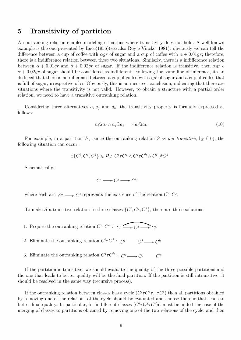
An outranking relation enables modeling situations where transitivity does not hold. A well-knownexample is the one presented by Luce(1956)(see also Roy e Vincke, 1981): obviously we can tell thedifference between a cup of coffee with αgr of sugar and a cup of coffee with α + 0.01gr; therefore,there is a indifference relation between these two situations. Similarly, there is a indifference relationbetween α + 0.01gr and α + 0.02gr of sugar. If the indifference relation is transitive, then αgr eα + 0.02gr of sugar should be considered as indifferent. Following the same line of inference, it candeduced that there is no difference between a cup of coffee with αgr of sugar and a cup of coffee thatis full of sugar, irrespective of α. Obviously, this is an incorrect conclusion, indicating that there aresituations where the transitivity is not valid. However, to obtain a structure with a partial orderrelation, we need to have a transitive outranking relation.
Considering three alternatives ai,aj and ak, the transitivity property is formally expressed asfollows:
aiℑaj ∧ ajℑak =⇒ aiℑak (10)
For example, in a partition Ps, since the outranking relation S is not transitive, by (10), thefollowing situation can occur:
∃{C i, Cj, Ck} ∈ Ps: CiτCj ∧ CjτCk ∧ C i 6 τCk
Schematically:
C i // Cj // Ck
where each arc C i // Cj represents the existence of the relation C iτCj.
To make S a transitive relation to three classes {C i, Cj, Ck}, there are three solutions:
1. Require the outranking relation C iτCk : C i //''
Cj // Ck
2. Eliminate the outranking relation C iτCj : C i Cj // Ck
3. Eliminate the outranking relation CjτCk : C i // Cj Ck
If the partition is transitive, we should evaluate the quality of the three possible partitions andthe one that leads to better quality will be the final partition. If the partition is still intransitive, itshould be resolved in the same way (recursive process).
If the outranking relation between classes has a cycle (C iτCjτ...τC i) then all partitions obtainedby removing one of the relations of the cycle should be evaluated and choose the one that leads tobetter final quality. In particular, for indifferent classes (C iτCjτC i)it must be added the case of themerging of classes to partitions obtained by removing one of the two relations of the cycle, and then
9

choose the best partition in terms of quality obtained.
Example
C1
��
C2
}}||||||||
��C3 C4
}}||||||||
C5
==||||||||
Figure 2: Preferred structure of P
Consider the partition P={C1, C2, C3, C4, C5} and the preference structure presented in Figure2.
In this structure there are two problems: the intransitivity of (C2, C4, C5) and a indifference ofpair (C4, C5). To solve the problem, and starting with indifference, there are three possible solutions:S1, S2 and S3 (Figure 3).
S1 S2 S3
C1
��
C2
}}||||||||
��
C1
��
C2
}}||||||||
��
C1
��
C2
zzuuuuuuuuuu
��
C3 C4
}}||||||||
C3 C4 C3 C4 ∪ C5
C5 C5
==||||||||
Figure 3: Possible solutions for intransitive partition Ps
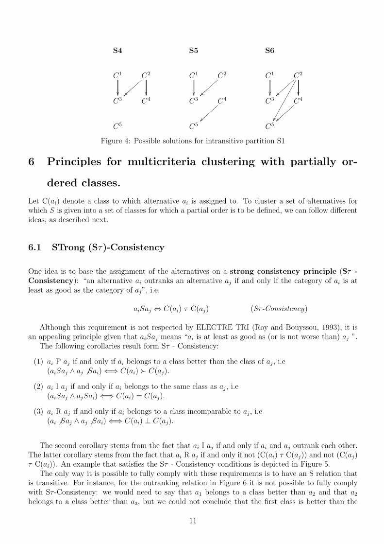
S2 and S3 are transitive partitions, but S1 does not verify the transitivity property. Now, apply-ing the same rule to S1 obtain transitive partitions S4, S5 and S6 (Figure 4).
Finally, we should evaluate the quality of the seven possible transitive partitions and the one thatleads to better quality will be the final partition.
10
S4 S5 S6
C1
��
C2
}}||||||||
��
C1
��
C2
}}||||||||
C1
��
C2
}}||||||||
��
��
C3 C4 C3 C4
}}||||||||
C3 C4
}}||||||||
C5 C5 C5
Figure 4: Possible solutions for intransitive partition S1
6 Principles for multicriteria clustering with partially or-
dered classes.
Let C(ai) denote a class to which alternative ai is assigned to. To cluster a set of alternatives forwhich S is given into a set of classes for which a partial order is to be defined, we can follow differentideas, as described next.
6.1 STrong (Sτ)-Consistency
One idea is to base the assignment of the alternatives on a strong consistency principle (Sτ -Consistency): “an alternative ai outranks an alternative aj if and only if the category of ai is atleast as good as the category of aj”, i.e.
aiSaj ⇔ C(ai) τ C(aj) (Sτ -Consistency)
Although this requirement is not respected by ELECTRE TRI (Roy and Bouyssou, 1993), it isan appealing principle given that aiSaj means “ai is at least as good as (or is not worse than) aj ”.
The following corollaries result form Sτ - Consistency:
(1) ai P aj if and only if ai belongs to a class better than the class of aj , i.e(aiSaj ∧ aj 6 Sai)⇐⇒ C(ai) ≻ C(aj).
(2) ai I aj if and only if ai belongs to the same class as aj , i.e(aiSaj ∧ ajSai)⇐⇒ C(ai) = C(aj).
(3) ai R aj if and only if ai belongs to a class incomparable to aj, i.e(ai 6 Saj ∧ aj 6 Sai)⇐⇒ C(ai) ⊥ C(aj).
The second corollary stems from the fact that ai I aj if and only if ai and aj outrank each other.The latter corollary stems from the fact that ai R aj if and only if not (C(ai) τ C(aj)) and not (C(aj)τ C(ai)). An example that satisfies the Sτ - Consistency conditions is depicted in Figure 5.
The only way it is possible to fully comply with these requirements is to have an S relation thatis transitive. For instance, for the outranking relation in Figure 6 it is not possible to fully complywith Sτ -Consistency: we would need to say that a1 belongs to a class better than a2 and that a2belongs to a class better than a3, but we could not conclude that the first class is better than the
11

Figure 5: Illustration of Sτ - Consistency
latter since a1 and a3 would be required to be in incomparable classes. Hence, we will next suggestless stringent forms of consistency.
Figure 6: Impossible to comply with Sτ - Consistency
6.2 Forms of Sτ-Consistency relaxed
Sτ -Consistency requires consistency from S to τ and vice-versa. Relaxing the Sτ -Consistency, weget two weak forms, which we call S-Consistency and τ -Consistency, resulting from splitting thetwo-way principle of equivalence into two one-way principles. We will first discuss these two formsof relaxation, and then we will introduce a third type of relaxation, which we call SSτ -Consistency,based on a different rationale.
A. S-Consistency
Considering S-Consistency, we base the assignment of the alternatives on the principle “if analternative ai outranks an alternative aj then the category of ai must be at least as good as thecategory of aj”, i.e.
aiSaj ⇒ C(ai) τ C(aj) (S-Consistency)
The following corollaries result form S-Consistency (proof omitted):
(1) if ai P aj then ai must belong to a class at least as better than the class of aj , i.e(aiSaj ∧ aj 6 Sai) =⇒ C(ai)τC(aj).
12
(2) if ai I aj then ai must belong the same class as aj , i.e(aiSaj ∧ ajSai) =⇒ C(ai) = C(aj).
(3) if ai R aj then ai and aj could belong to any class.
The third corollary stems from the fact that if none of the alternatives outranks the other, thennothing can be concluded.
Given a partial order of classes, the S-Consistency principle can be rephrased as stating that “al-ternatives belonging to a given category cannot be outranked by any alternative belonging to a loweror incomparable category, and cannot outrank any alternative belonging to a higher or incomparablecategory”, i.e.,
( C(ai) 6 τC(aj)⇒ ai 6 Saj) ⇐⇒ [(C(aj) ≻ C(ai) ∨ C(ai) ⊥ C(aj))⇒ ai 6 Saj ]
As a consequence, we obtain the three following corollaries:
(4) if C(ai) is better than C(aj) then we can have ai P aj or aj R ai.
(5) if C(ai) is incomparable to C(aj) then must have ai R aj.
(6) if C(ai) = C(aj) then we can have ai P aj, ai I aj, or even ai R aj.
In accordance with the principle S-Consistency, the following inconsistencies should not occur:
(1) aiPaj ∧ (C(aj) ≻ C(ai) ∨ C(aj) ⊥ C(ai)) (S-Inconsistencies)
(2) aiIaj ∧ (C(ai) ≻ C(aj) ∨ C(aj) ≻ C(ai) ∨ C(aj) ⊥ C(ai))
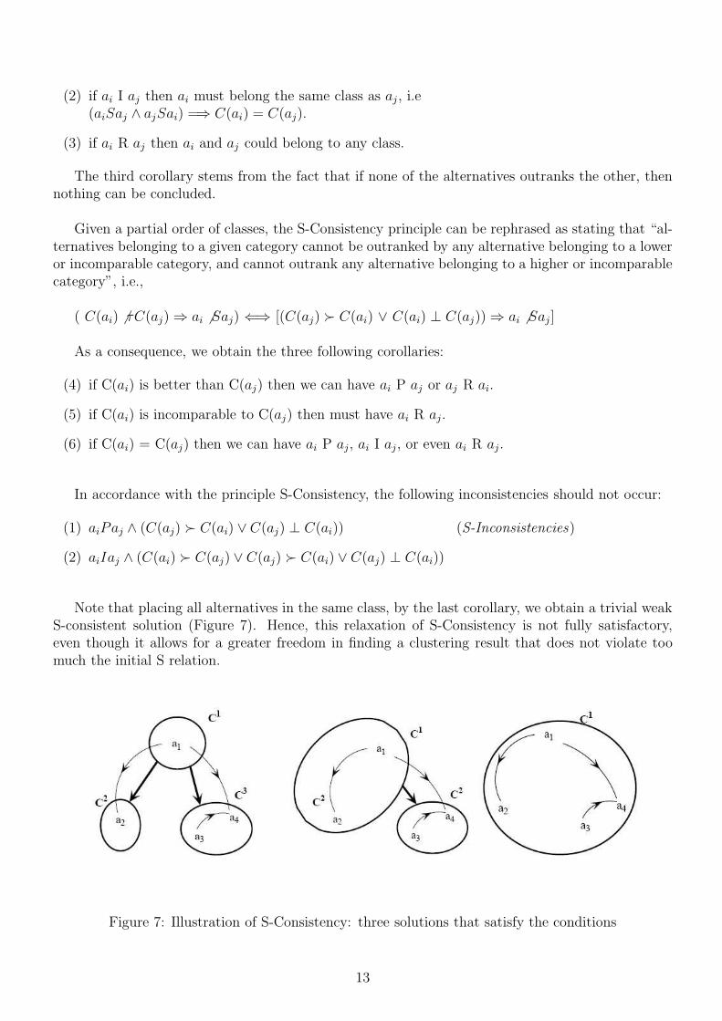
Note that placing all alternatives in the same class, by the last corollary, we obtain a trivial weakS-consistent solution (Figure 7). Hence, this relaxation of S-Consistency is not fully satisfactory,even though it allows for a greater freedom in finding a clustering result that does not violate toomuch the initial S relation.
Figure 7: Illustration of S-Consistency: three solutions that satisfy the conditions
13

Note that, if there exists a cycle in the outranking relation (aiSajSakS...Sai), then S-Consistencyalso implies that all the alternatives involved in the cycle must be placed in the same category. Thisfollows the philosophy of ELECTRE I and this is the principle proposed by Rocha and Dias (2008)for an interactive algorithm for ordinal classification.
B. τ - Consistency
Considering τ - Consistency, we base the assignment of the alternatives on the principle “ if thecategory of ai is at least as good as the category of aj then the alternative ai outranks the alternativeaj ”:
C(ai) τ C(aj) ⇒ ai S aj ( τ - Consistency)
The following corollaries result form τ -Consistency:
(1) if C(ai) is better than C(aj) then we can have ai P aj or ai I aj .
(2) if C(ai) is incomparable to C(aj) we can have ai P aj , aj P ai, ai R aj, or even ai I aj .
(3) if C(ai) = C(aj) then we must have ai I aj .
The τ -Consistency principle can be rephrased as stating that “alternatives that do not outrank ano-ther alternatives, belong to a lower or incomparable category than that of the latter”, i.e.,
(ai 6 Saj ⇒ C(ai) 6 τC(aj)) ⇐⇒ [(ai 6 Saj)⇒ (C(aj) ≻ C(ai) ∨ C(ai) ⊥ C(aj))]
As a consequence, we obtain the three following corollaries:
(4) if ai P aj then ai must belong to a class either incomparable or better than the class of aj .
(5) if ai I aj then ai and aj can belong to any class.
(6) if ai R aj then ai and aj must belong to incomparable classes.
In accordance with the principle τ -Consistency, the following inconsistencies can occur:
• aiPaj ∧ (C(aj) ≻ C(ai) ∨ C(aj) = C(ai)) (τ -Inconsistencies)
• aiRaj ∧ (C(aj) = C(ai) ∨ C(ai) ≻ C(aj) ∨ C(aj) ≻ C(ai))
Note that, by corollary 2, if each class has only one alternative and the classes are declared allincomparable then this would be a τ -Consistent solution. Again, this relaxation of Sτ -Consistency isnot fully satisfactory, even though it allows for a greater freedom in finding a clustering result thatdoes not violate too much the initial S relation.
C. Semi-STrong (SSτ) - Consistency
Table 2 summarizes what has been discussed so far. Given two alternatives ai and aj belongingto classes C(ai) and C(aj), it shows the possible combinations that are inconsistent according to
14
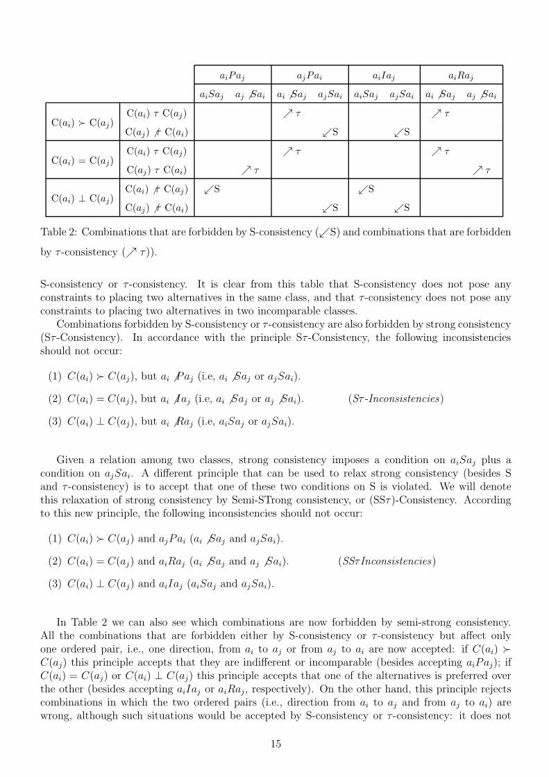
aiPaj ajPai aiIaj aiRaj
aiSaj aj 6 Sai ai 6 Saj ajSai aiSaj ajSai ai 6 Saj aj 6 Sai
C(ai) ≻ C(aj)C(ai) τ C(aj) ր τ ր τ
C(aj) 6 τ C(ai) ւS ւS
C(ai) = C(aj)C(ai) τ C(aj) ր τ ր τ
C(aj) τ C(ai) ր τ ր τ
C(ai) ⊥ C(aj)C(ai) 6 τ C(aj) ւS ւS
C(aj) 6 τ C(ai) ւS ւS
Table 2: Combinations that are forbidden by S-consistency (ւS) and combinations that are forbidden
by τ -consistency (ր τ)).
S-consistency or τ -consistency. It is clear from this table that S-consistency does not pose anyconstraints to placing two alternatives in the same class, and that τ -consistency does not pose anyconstraints to placing two alternatives in two incomparable classes.
Combinations forbidden by S-consistency or τ -consistency are also forbidden by strong consistency(Sτ -Consistency). In accordance with the principle Sτ -Consistency, the following inconsistenciesshould not occur:
(1) C(ai) ≻ C(aj), but ai 6 Paj (i.e, ai 6 Saj or ajSai).
(2) C(ai) = C(aj), but ai 6 Iaj (i.e, ai 6 Saj or aj 6 Sai). (Sτ -Inconsistencies)
(3) C(ai) ⊥ C(aj), but ai 6 Raj (i.e, aiSaj or ajSai).
Given a relation among two classes, strong consistency imposes a condition on aiSaj plus acondition on ajSai. A different principle that can be used to relax strong consistency (besides Sand τ -consistency) is to accept that one of these two conditions on S is violated. We will denotethis relaxation of strong consistency by Semi-STrong consistency, or (SSτ)-Consistency. Accordingto this new principle, the following inconsistencies should not occur:
(1) C(ai) ≻ C(aj) and ajPai (ai 6 Saj and ajSai).
(2) C(ai) = C(aj) and aiRaj (ai 6 Saj and aj 6 Sai). (SSτInconsistencies)
(3) C(ai) ⊥ C(aj) and aiIaj (aiSaj and ajSai).
In Table 2 we can also see which combinations are now forbidden by semi-strong consistency.All the combinations that are forbidden either by S-consistency or τ -consistency but affect onlyone ordered pair, i.e., one direction, from ai to aj or from aj to ai are now accepted: if C(ai) ≻C(aj) this principle accepts that they are indifferent or incomparable (besides accepting aiPaj); ifC(ai) = C(aj) or C(ai) ⊥ C(aj) this principle accepts that one of the alternatives is preferred overthe other (besides accepting aiIaj or aiRaj, respectively). On the other hand, this principle rejectscombinations in which the two ordered pairs (i.e., direction from ai to aj and from aj to ai) arewrong, although such situations would be accepted by S-consistency or τ -consistency: it does not
15
accept indifferent alternatives in incomparable classes (which τ -consistency accepts), and it does notaccept incomparable alternatives the same class (which S-consistency accepts).
In this paper, we present an extension of the agglomerative hierarchical algorithm to the multicri-teria framework, based on the (SSτ)-Consistency, which seems to be the best principle for groupingalternatives into partially ordered classes, given a possibly intransitive outranking relation S.
7 Measure of similarity between classes
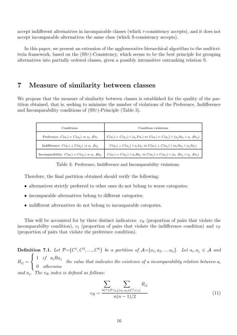
We propose that the measure of similarity between classes is established for the quality of the par-tition obtained, that is, seeking to minimize the number of violations of the Preference, Indifferenceand Incomparability conditions of (SSτ)-Principle (Table 3).
Conditions Condition violations
Preference: C(ai) ≻ C(aj) ⇒ aj 6 Pai C(ai) ≻ C(aj ) ∧ (ajPai) ⇔ C(ai) ≻ C(aj ) ∧ (ajSai ∧ ai 6 Saj)
Indifference: C(ai) ⊥ C(aj ) ⇒ ai 6 Iaj C(ai) ⊥ C(aj) ∧ aiIaj ⇔ C(ai) ⊥ C(aj ) ∧ (aiSaj ∧ ajSai)
Incomparability: C(ai) = C(aj ) ⇒ ai 6 Raj C(ai) = C(aj) ∧ aiRaj ⇔ C(ai) = C(aj) ∧ (ai 6 Saj ∧ aj 6 Sai)
Table 3: Preference, Indifference and Incomparability violations.
Therefore, the final partition obtained should verify the following:
• alternatives strictly preferred to other ones do not belong to worse categories;
• incomparable alternatives belong to different categories;
• indifferent alternatives do not belong to incomparable categories.
This will be accounted for by three distinct indicators: vR (proportion of pairs that violate theincomparability condition), vI (proportion of pairs that violate the indifference condition) and vP(proportion of pairs that violate the preference condition).
Definition 7.1. Let P={C1, C2, ...., Ck} be a partition of A={a1, a2, ..., an}. Let ai, aj ∈ A and
Rij =
1 if aiRaj
0 otherwisethe value that indicates the existence of a incomparability relation between ai
and aj. The vR index is defined as follows:
vR =
∑
∀Ct∈P
∑
(i,j):ai,aj∈Ct,i<j
Rij
n(n− 1)/2(11)
16
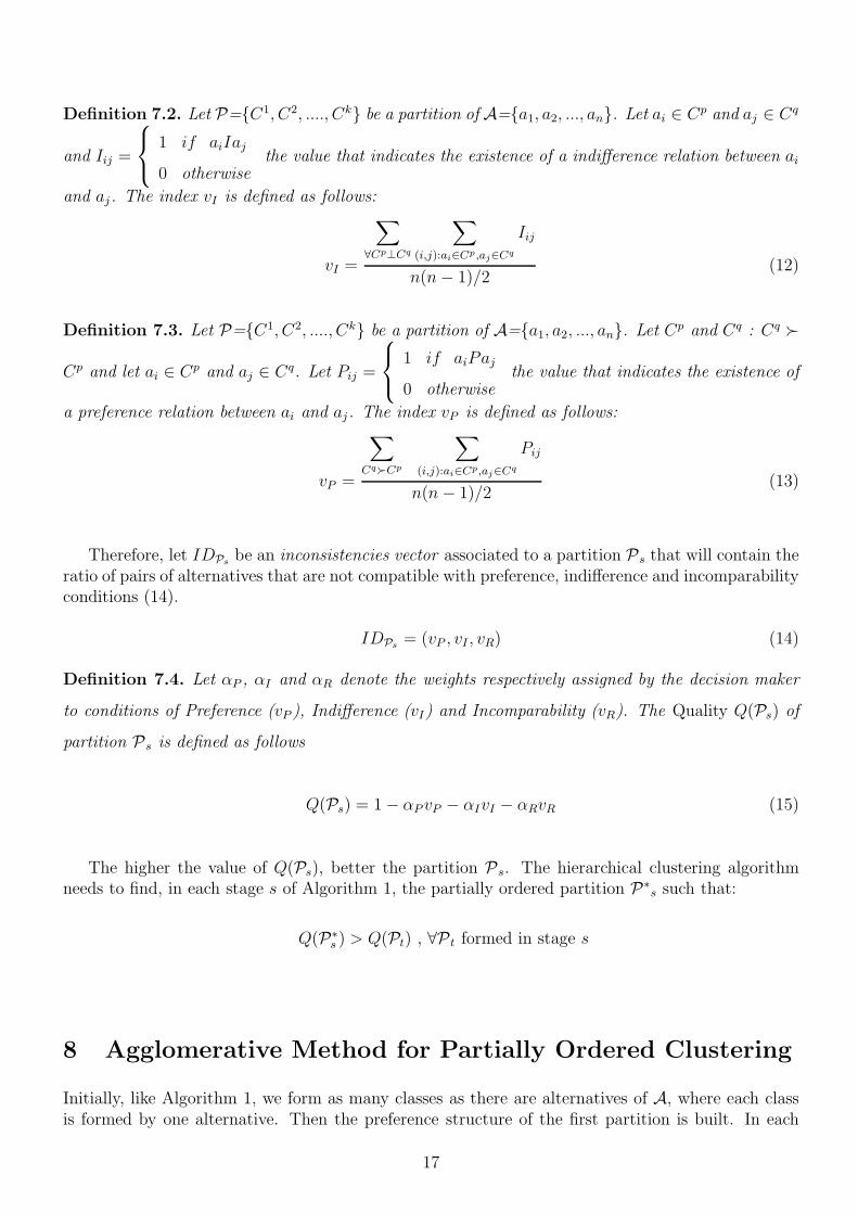
Definition 7.2. Let P={C1, C2, ...., Ck} be a partition of A={a1, a2, ..., an}. Let ai ∈ Cp and aj ∈ Cq
and Iij =
1 if aiIaj
0 otherwisethe value that indicates the existence of a indifference relation between ai
and aj. The index vI is defined as follows:
vI =
∑
∀Cp⊥Cq
∑
(i,j):ai∈Cp,aj∈Cq
Iij
n(n− 1)/2(12)
Definition 7.3. Let P={C1, C2, ...., Ck} be a partition of A={a1, a2, ..., an}. Let Cp and Cq : Cq ≻
Cp and let ai ∈ Cp and aj ∈ Cq. Let Pij =
1 if aiPaj
0 otherwisethe value that indicates the existence of
a preference relation between ai and aj. The index vP is defined as follows:
vP =
∑
Cq≻Cp
∑
(i,j):ai∈Cp,aj∈Cq
Pij
n(n− 1)/2(13)
Therefore, let IDPsbe an inconsistencies vector associated to a partition Ps that will contain the
ratio of pairs of alternatives that are not compatible with preference, indifference and incomparabilityconditions (14).
IDPs= (vP , vI , vR) (14)
Definition 7.4. Let αP , αI and αR denote the weights respectively assigned by the decision maker
to conditions of Preference (vP ), Indifference (vI) and Incomparability (vR). The Quality Q(Ps) of
partition Ps is defined as follows
Q(Ps) = 1− αP vP − αIvI − αRvR (15)
The higher the value of Q(Ps), better the partition Ps. The hierarchical clustering algorithmneeds to find, in each stage s of Algorithm 1, the partially ordered partition P∗
s such that:
Q(P∗s ) > Q(Pt) , ∀P t formed in stage s
8 Agglomerative Method for Partially Ordered Clustering
Initially, like Algorithm 1, we form as many classes as there are alternatives of A, where each classis formed by one alternative. Then the preference structure of the first partition is built. In each
17
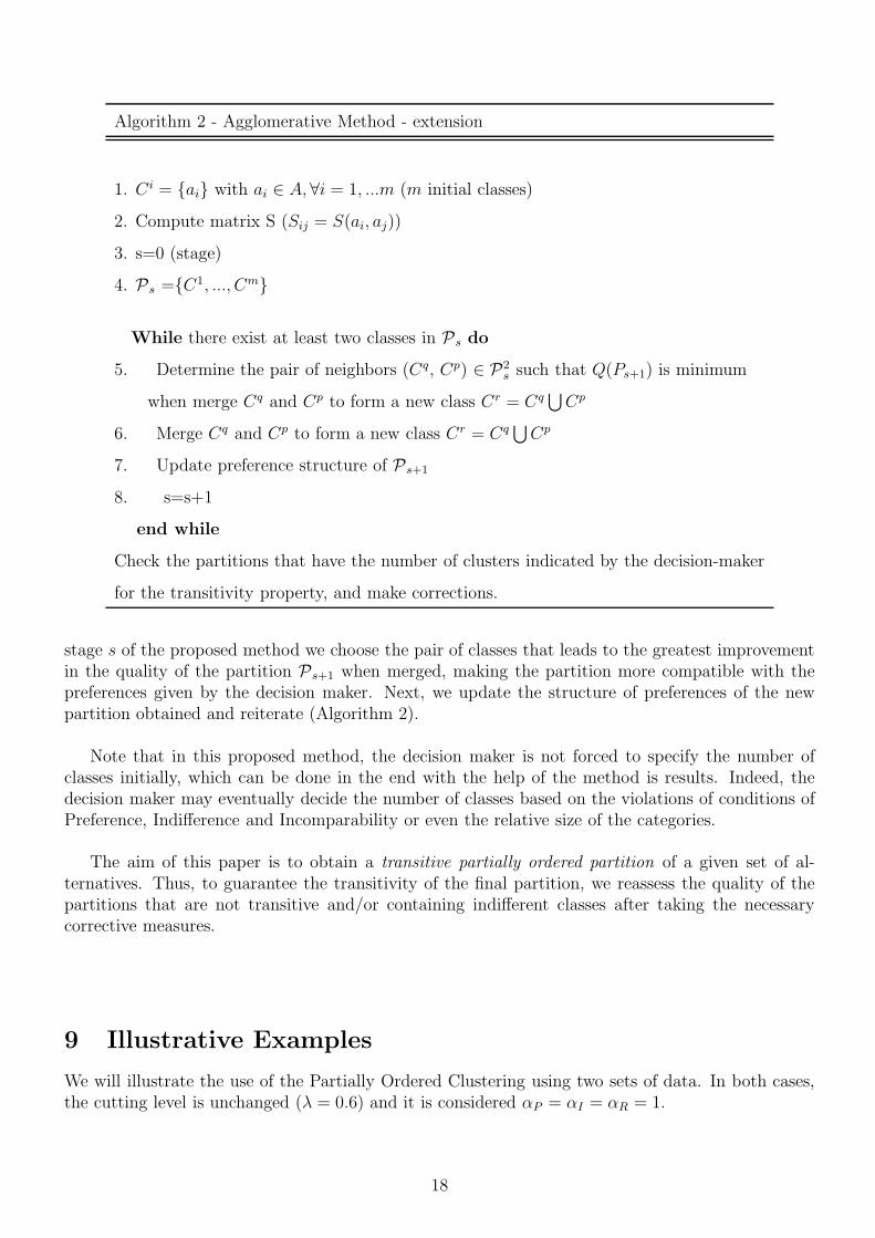
Algorithm 2 - Agglomerative Method - extension
1. C i = {ai} with ai ∈ A, ∀i = 1, ...m (m initial classes)
2. Compute matrix S (Sij = S(ai, aj))
3. s=0 (stage)
4. Ps ={C1, ..., Cm}
While there exist at least two classes in Ps do
5. Determine the pair of neighbors (Cq, Cp) ∈ P2s such that Q(Ps+1) is minimum
when merge Cq and Cp to form a new class Cr = Cq⋃
Cp
6. Merge Cq and Cp to form a new class Cr = Cq⋃
Cp
7. Update preference structure of Ps+1
8. s=s+1
end while
Check the partitions that have the number of clusters indicated by the decision-maker
for the transitivity property, and make corrections.
stage s of the proposed method we choose the pair of classes that leads to the greatest improvementin the quality of the partition Ps+1 when merged, making the partition more compatible with thepreferences given by the decision maker. Next, we update the structure of preferences of the newpartition obtained and reiterate (Algorithm 2).
Note that in this proposed method, the decision maker is not forced to specify the number ofclasses initially, which can be done in the end with the help of the method is results. Indeed, thedecision maker may eventually decide the number of classes based on the violations of conditions ofPreference, Indifference and Incomparability or even the relative size of the categories.
The aim of this paper is to obtain a transitive partially ordered partition of a given set of al-ternatives. Thus, to guarantee the transitivity of the final partition, we reassess the quality of thepartitions that are not transitive and/or containing indifferent classes after taking the necessarycorrective measures.
9 Illustrative Examples
We will illustrate the use of the Partially Ordered Clustering using two sets of data. In both cases,the cutting level is unchanged (λ = 0.6) and it is considered αP = αI = αR = 1.
18

9.1 First example
Let us consider in a first example the data from an application for sorting stocks listed in the AthensStock Exchange (Hurson and Zopounidis, 1997), namely 20 alternatives from the commercial sector,which were evaluated on 6 criteria (Table 1). The criteria names are not relevant here, therefore wewill note only that all criteria are to be maximized, except g3(.), where the lower the values, the better.
g1 g2 g3 g4 g5 g6 g1 g2 g3 g4 g5 g6
a0 0,82 0,45 0,26 -4,7 -100 0,45 a10 0,8 0,58 0,62 13,7 34,6 1,54
a1 0,41 0,63 0,03 2,28 -20 2,04 a11 1,23 0,37 0,64 8,97 45,9 0,96
a2 0,57 0,2 0,1 6,08 -33,3 1,08 a12 0,24 0,28 0,73 -1,75 0 0,72
a3 0,24 0,02 0,08 2,41 -53,5 0,62 a13 0,26 0,65 0,58 4,88 7,14 0,9
a4 0 0,46 0,62 5,04 -76,5 3,02 a14 1,1 0,76 0,54 0,29 0 0,73
a5 0,93 0,02 0,14 2,82 6,38 0,72 a15 1,79 0,55 0,73 5,88 -100 2,69
a6 0,01 0,69 0,77 7,55 -40 3,23 a16 1,02 1,06 0,82 5,5 6,38 0,73
a7 0,86 0,86 0,86 4,28 3,71 0,57 a17 1,32 1,12 0,94 12,06 -61 2,69
a8 2,16 0,6 0,12 2,11 56,3 0,51 a18 1,36 0,04 1,02 1,79 110 2,31
a9 1,24 0,12 0,62 11,65 12,5 1,17 a19 0,57 0,17 0,23 -11,5 0 0,52
Table 4: Evaluations on six criteria for 20 stocks.
We will use the original values (Hurson and Zopounidis, 1997) for the indifference and preferencethresholds (Table 3), but we will use veto thresholds that are not as tight as the original ones. Thisoccurs, in this particular example, because the original values for the veto thresholds led to manyveto situations, which would imply having in the results either a large number of violations or a largenumber of categories. We used λ =0.6 and uj = pj .
g1 g2 g3 g4 g5 g6
qj 0,05 0,05 0 0,1 8,72 0,05
pj 0,25 0,2 0,2 0,5 10 0,25
vj 20 10 10 100 180 2,75
Table 5: Indifference, preference and veto thresholds.
Since the original data set (Hurson and Zopounidis, 1997) does not indicate any information aboutcriteria importance, all criteria are considered to have the same weight, i.e., ki = 1/6, i ∈ {1, ..., 6}.
Evaluating the set of these 20 alternatives based on their performance, criteria thresholds andweights, of the 190 pairs of alternatives studied (n(n−1)
2, n = 20), 121 (63.7%) verified the relation
of Preference, 8 (4.2%) verified the relation of Indifference and 61 (32.1%) verified the relation ofIncomparability.
As we can see in Figure 8, only for partitions with at least 12 classes we get a final qualityQ*=100%, which, given the number of alternatives, may be not a satisfactory solution. Consideringthat the decision maker is only interested in solutions with less than 7 classes (which is reasonabletaking into account that |A| =20), the results obtained by applying Algorithm 2, are shown in Table6.
In this example, all partitions are transitive. If the decision maker chooses k=5 classes as a goodsolution (the quality does not improve significantly from 5 classes), we obtain a partition with aquality of 97.37% resulting from 0% of violations of the Preference conditions, 0.53% of Indifferenceand 1.58% of Incomparability, with
• C1 = {a1, a2, a4, a7, a19},
19

0 1 2 3 4 5 6 7 8 9 10 11 12 13 1488
90
92
94
96
98
100
nr. classes
Qua
lity
(%)
Figure 8: Partition quality as a function of the number of classes (Example 1).
k Transitivity Quality Inconsistences vector Structure
6 X 97.89 (0 0 0.0211 ) © © 22© **© **© // ©
5 X 97.37 (0 0.0053 0.0211) © © 22© **© // ©
4 X 96.32 (0 0.0053 0.0316) © © **© // ©
3 X 94.21 (0 0.0053 0.0526) © © // ©
2 X 88.95 (0 0.0053 0.1053) © ©
1 X 67.89 (0 0 0.3211 )
Table 6: Partitions Quality with SSτ -Consistency
• C2 = {a3, a6, a8, a13, a14, a20},
• C3 = {a5, a18},
• C4 = {a9, a11, a16} and
• C5 = {a10, a12, a15, a17}.
From the outranking degrees between classes (Table 7) we obtained the partially ordered andtransitive partition presented in Figure 9.
20

C1 C2 C3 C4 C5
C1 0 0.3333 0.2000 0.1333 0.1000
C2 0.3333 0 0 0 0.1250
C3 0.4000 0.5833 0 0.3333 0.3750
C4 0.4667 0.7222 0 0 0.5833
C5 0.4000 0.9167 0 0 0
Table 7: Outranking degree sij within (C i, Cj), i=1..5
C1 C4
��
C3
��
C5
��
C2
Figure 9: Final Partition
9.2 Second example
We will now present a second example with more alternatives to sort. We will use an example fromYu (1992), referring to the evaluation of 100 alternatives to be sorted, based on their performanceson 7 criteria to be minimized.
We will consider as fixed the weights, indifference, preference, discordance, and veto thresholdsassociated with each criterion, indicated in Table 5. We allow for discordance to occur, although wehave chosen values for uj and vj that do not allow veto situations to occur frequently when comparingthe alternatives.
g1 g2 g3 g4 g5 g6 g7
qj 0.65 1.7 1.7 1.7 1.7 1.7 2.3
pj 1.31 3.45 3.45 3.45 3.45 3.45 4.7
uj 1.95 10.4 10.4 10.4 10.4 10.5 18.7
vj 1.95 100 100 100 100 100 18.7
kj 0.24 0.12 0.12 0.12 0.12 0.12 0.16
Table 8: Thresholds and weights associated with the criteria.
Evaluating the set of alternatives based on their performance, weights, criteria thresholds (with
vj and λ = 0.6), of the 4950 pairs of alternatives studied (n(n−1)2
, n = 100), 2967 (59.9%) verify therelation of Preference, 364 (7.4%) verify the relation of Indifference, and 1619 (32.7%) verify therelation of Incomparability.
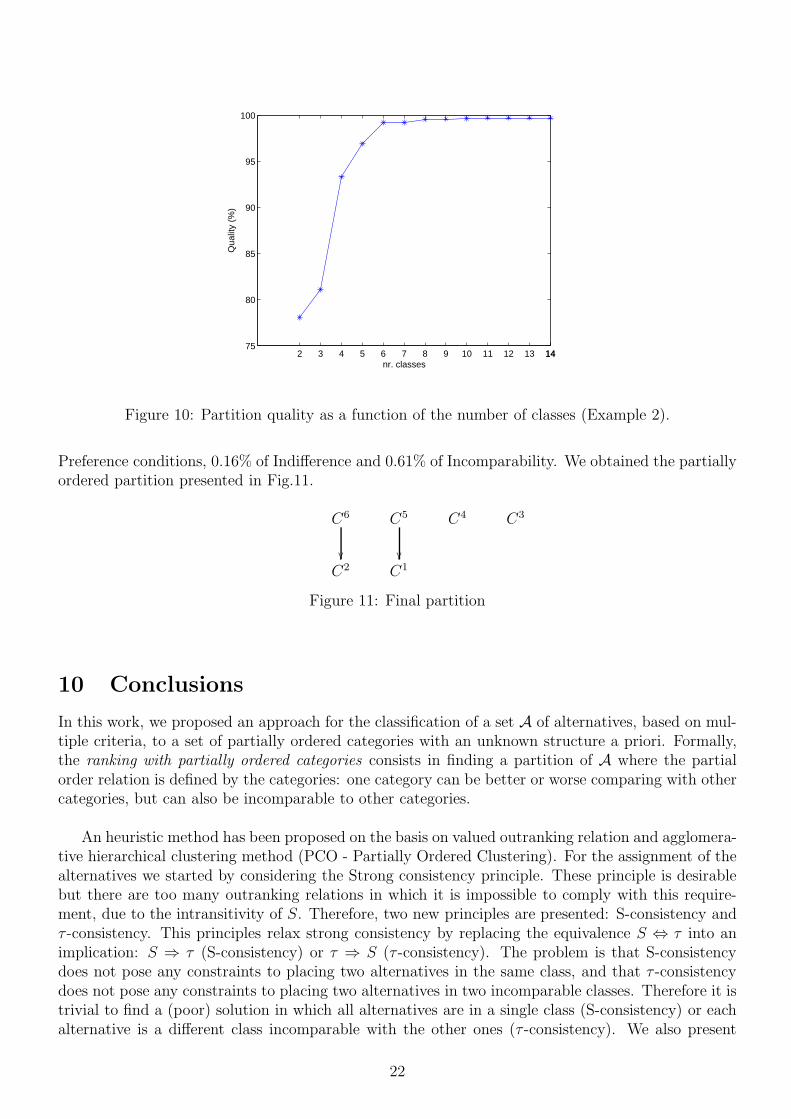
Considering that the decision maker is interested only in solutions with less than 8 classes, theresults of the merged classes that cause the better quality of the partition are presented in Table 9.Figure 10 depicts how the number of classes impacts on partition quality. As we can see, a goodsolution can be k = 6 because the quality of the partitions with more than 6 classes is not significantlybetter .
In this example, all partitions are transitive. If the decision maker chooses k=6 classes as agood solution, we obtain a partition with a quality of 99.23% resulting from 0% of violations of the
21
2 3 4 5 6 7 8 9 10 11 12 13 141475
80
85
90
95
100
nr. classes
Qua
lity
(%)
Figure 10: Partition quality as a function of the number of classes (Example 2).
Preference conditions, 0.16% of Indifference and 0.61% of Incomparability. We obtained the partiallyordered partition presented in Fig.11.
C6
��
C5
��
C4 C3
C2 C1
Figure 11: Final partition
10 Conclusions
In this work, we proposed an approach for the classification of a set A of alternatives, based on mul-tiple criteria, to a set of partially ordered categories with an unknown structure a priori. Formally,the ranking with partially ordered categories consists in finding a partition of A where the partialorder relation is defined by the categories: one category can be better or worse comparing with othercategories, but can also be incomparable to other categories.
An heuristic method has been proposed on the basis on valued outranking relation and agglomera-tive hierarchical clustering method (PCO - Partially Ordered Clustering). For the assignment of thealternatives we started by considering the Strong consistency principle. These principle is desirablebut there are too many outranking relations in which it is impossible to comply with this require-ment, due to the intransitivity of S. Therefore, two new principles are presented: S-consistency andτ -consistency. This principles relax strong consistency by replacing the equivalence S ⇔ τ into animplication: S ⇒ τ (S-consistency) or τ ⇒ S (τ -consistency). The problem is that S-consistencydoes not pose any constraints to placing two alternatives in the same class, and that τ -consistencydoes not pose any constraints to placing two alternatives in two incomparable classes. Therefore it istrivial to find a (poor) solution in which all alternatives are in a single class (S-consistency) or eachalternative is a different class incomparable with the other ones (τ -consistency). We also present
22
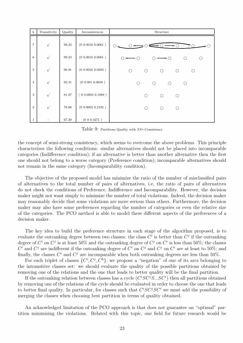
k Transitivity Quality Inconsistences Structure
7√
99.23 (0 0.0016 0.0061 ) © © ©oojj // 22,,© // © © ©
6√
99.23 (0 0.0016 0.0061 ) © ©oo © // © © ©
5√
96.91 (0 0.0016 0.0293 ) © © © © ©
4√
93.31 (0 0.001 0.0659 ) © © © ©
3√
81.07 ( 0 0.0004 0.1889 ) © © ©
2√
78.06 (0 0.0002 0.2192 ) © © ©
1 - 67.29 (0 0 0.3271 )
Table 9: Partitions Quality with SSτ -Consistency
the concept of semi-strong consistency, which seems to overcome the above problems. This principlecharacterizes the following conditions: similar alternatives should not be placed into incomparablecategories (Indifference condition); if an alternative is better than another alternative then the firstone should not belong to a worse category (Preference condition); incomparable alternatives shouldnot remain in the same category (Incomparability condition).
The objective of the proposed model has minimize the ratio of the number of misclassified pairsof alternatives to the total number of pairs of alternatives, i.e, the ratio of pairs of alternativesdo not check the conditions of Preference, Indifference and Incomparability. However, the decisionmaker might not want simply to minimize the number of total violations. Indeed, the decision makermay reasonably decide that some violations are more serious than others. Furthermore, the decisionmaker may also have some preferences regarding the number of categories or even the relative sizeof the categories. The PCO method is able to model these different aspects of the preferences of adecision maker.
The key idea to build the preference structure in each stage of the algorithm proposed, is toevaluate the outranking degree between two classes: the class C i is better than Cj if the outrankingdegree of C i on Cj is at least 50% and the outranking degree of Cj on C i is less than 50%; the classesC i and Cj are indifferent if the outranking degree of C i on Cj and Cj on C i are at least to 50%; andfinally, the classes C i and Cj are incomparable when both outranking degrees are less than 50%.
For each triplet of classes {C i, Cj, Ck}, we propose a “negation” of one of its arcs belonging tothe intransitive classes set: we should evaluate the quality of the possible partitions obtained byremoving one of the relations and the one that leads to better quality will be the final partition.
If the outranking relation between classes has a cycle (C iSCjS...SC i) then all partitions obtainedby removing one of the relations of the cycle should be evaluated in order to choose the one that leadsto better final quality. In particular, for classes such that C iSCjSC i we must add the possibility ofmerging the classes when choosing best partition in terms of quality obtained.
An acknowledged limitation of the PCO approach is that does not guarantee an “optimal” par-tition minimizing the violations. Related with this topic, one field for future research would be
23
the development of optimization approaches to match the preferences of a decision maker. Thecomparisons with other ways for multicriteria clustering is another field for future research.
References
[1] Brans, J.P, Vincke, Ph (1985).A preference ranking organization method. Management Science31(6):647-656.
[2] De Smet, Y., Montano, G.L. (2004). Towards multicriteria clustering: an extension of the k-means algorithm. European Journal of Operational Research 158(2) : 390-398
[3] Dias, L.C., C. Lamboray (2010), Extensions of the prudence principle to exploit a valued out-ranking relation, European Journal of Operational Research, Vol. 201, No. 3, 828-837.
[4] Doumpos, M., Zopounidis, C. (2002), Multicriteria Decision Aid Classification Methods, KluwerAcademic Publishers, Dordrecht.
[5] Fernandez E., Navarro J., Bernal S. (2010). Handling multicriteria preferences in cluster analysis.European Journal of Operational Research 202 : 819-827.
[6] Figueira, J., De Smet, Y., Brans, JP (2004). Promethee for MCDA Classification and Sortingproblems: Promethee TRI and Promethee CLUSTER. Technical Report TR/SMG/2004-02.Universite Libre de Bruxelles.
[7] Fisher, D. (1987). Knowledge acquisition via incremental conceptual clustering. Machine Learn-ing, 2, 139-172.
[8] Guha, S., Rastogi, R., and Shim, K. (1998). CURE: An efficient clustering algorithm for largedatabases. In Proceedings of the ACM SIGMOD Conference, 73-84, Seattle, WA.
[9] Jain, A.K., Dubes, R.C. (1988). Algorithms for Clustering Data. Prentice-Hall advanced refer-ence series. Prentice-Hall,Inc., Upper Saddle River, NJ.
[10] Karypis, G., Han, E.H., Kumar, V. (1999). CHAMELEON: A hierarchical clustering algorithmusing dynamic modeling, COMPUTER, 32, 68-75.
[11] Kaufman, L., Rousseeuw, P. (1990). Finding Groups in Data : An introduction to ClusterAnalysis. John Wiley and Sons, New York.
[12] Keeney, R. L., Raiffa, H. (1993), Decisions with multiple objectives: preferences and valuetradeoff, Cambridge University Press, Cambridge.
[13] Mousseau, V., Dias, L. (2004), Valued outranking relations in ELECTRE providing manageabledisaggregation procedures. European Journal of Operational Research,156(2),467-482.
[14] Mousseau, V., Slowinski, R. (1998), Inferring an ELECTRE-TRI model from assignement ex-amples. Journal of Global Optimization 12(2), 157-174.
[15] Nemery,P.;De Smet, Y.(2005). Multicriteria Ordered Clustering. Technical ReportTR/SMG/2005-003, SMG, Universit Libre de Bruxelles, 2005.
[16] Roy B. (1978), ELECTRE III: Un algorithme de classements fonde sur une representation flouedes preferences de criteres multiples. Cahiers du CERO, 20(1):3-24.
24
[17] Roy B., Bouyssou D. (1993), Aide multicritere a la decision : Methodes et cas. Economica,Paris.
[18] Roy B.(1991), The outranking approach and the foundations of ELECTRE methods. Theoryand Decision 31, 49-73.
[19] Roy B., Bouyssou D. (1993), Aide multicritre la dcision : Mthodes et cas. Economica, Paris.
[20] Saaty, T.L.(1980), The analytic hierarchy process, McGraw-Hill, New York.
[21] Saaty, T.L.(1996), Decision making with dependence and feedback: the analytic network process.RWS Publications, Pittsburg.
[22] Sibson, R. (1973). SLINK: An optimally efficient algorithm for the single link cluster method.Computer Journal, 16, 30-34.
[23] Vincke, P.(1992). Multicriteria Decision-Aid. New York: J.Wiley.
[24] Yu, W.(1992), Aide multicritre la dcision dans le cadre de la problmatique du tri: concepts,mthodes et applications. Doctoral dissertation, Universit Paris-Dauphine.
25