Poblano v1.0: A Matlab Toolbox for Gradient-Based Optimizationprod.sandia.gov/techlib/access-control.cgi/2010/101422.pdf · Gradient-Based Optimization ... a Matlab toolbox for solving

SANDIA REPORTSAND2010-1422SAND2010-XXXXUnlimited ReleasePrinted March 2010

Poblano v1.0: A Matlab Toolbox forGradient-Based Optimization

Daniel M. Dunlavy, Tamara G. Kolda, and Evrim Acar

Prepared bySandia National LaboratoriesAlbuquerque, New Mexico 87185 and Livermore, California 94550

Sandia is a multiprogram laboratory operated by Sandia Corporation,a Lockheed Martin Company, for the United States Department of Energy’sNational Nuclear Security Administration under Contract DE-AC04-94-AL85000.

Approved for public release; further dissemination unlimited.

Issued by Sandia National Laboratories, operated for the United States Department of Energyby Sandia Corporation.

NOTICE: This report was prepared as an account of work sponsored by an agency of the UnitedStates Government. Neither the United States Government, nor any agency thereof, nor anyof their employees, nor any of their contractors, subcontractors, or their employees, make anywarranty, express or implied, or assume any legal liability or responsibility for the accuracy,completeness, or usefulness of any information, apparatus, product, or process disclosed, or rep-resent that its use would not infringe privately owned rights. Reference herein to any specificcommercial product, process, or service by trade name, trademark, manufacturer, or otherwise,does not necessarily constitute or imply its endorsement, recommendation, or favoring by theUnited States Government, any agency thereof, or any of their contractors or subcontractors.The views and opinions expressed herein do not necessarily state or reflect those of the UnitedStates Government, any agency thereof, or any of their contractors.

Printed in the United States of America. This report has been reproduced directly from the bestavailable copy.

Available to DOE and DOE contractors fromU.S. Department of EnergyOffice of Scientific and Technical InformationP.O. Box 62Oak Ridge, TN 37831

Telephone: (865) 576-8401Facsimile: (865) 576-5728E-Mail: [email protected] ordering: http://www.osti.gov/bridge

Available to the public fromU.S. Department of CommerceNational Technical Information Service5285 Port Royal RdSpringfield, VA 22161

Telephone: (800) 553-6847Facsimile: (703) 605-6900E-Mail: [email protected] ordering: http://www.ntis.gov/help/ordermethods.asp?loc=7-4-0#online

DE

PA

RT

MENT OF EN

ER

GY

• • UN

IT

ED

STATES OFA

M

ER

IC

A

2

SAND2010-1422XXXXUnlimited Release

Printed March 2010

Poblano v1.0: A Matlab Toolbox for Gradient-Based

Optimization

Daniel M. DunlavyComputer Science & Informatics Department

Sandia National Laboratories, Albuquerque, NM 87123-1318Email: [email protected]

Tamara G. Kolda and Evrim AcarInformation and Decision Sciences Department

Sandia National LaboratoriesLivermore, CA 94551-9159

Email: [email protected], [email protected]

Abstract

We present Poblano v1.0, a Matlab toolbox for solving gradient-based unconstrained optimizationproblems. Poblano implements three optimization methods (nonlinear conjugate gradients, limited-memory BFGS, and truncated Newton) that require only first order derivative information. In thispaper, we describe the Poblano methods, provide numerous examples on how to use Poblano, and presentresults of Poblano used in solving problems from a standard test collection of unconstrained optimizationproblems.

3

http://www.cs.sandia.gov/~dmdunla/

http://csmr.ca.sandia.gov/~tgkolda

http://csmr.ca.sandia.gov/~eacart

Acknowledgments

We thank Dianne O’Leary for providing the Matlab translation of the MINPACK implementation of theMore-Thuente line search. This product includes software developed by the University of Chicago, as Op-erator of Argonne National Laboratory. This work was fully supported by Sandia’s Laboratory DirectedResearch & Development (LDRD) program.

4

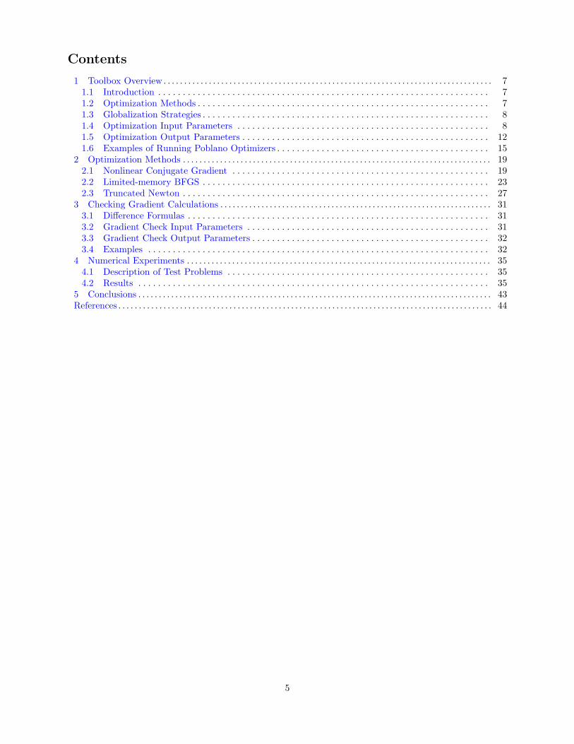
Contents

1 Toolbox Overview . . . . . . . . . . . . . . . . . . . . . . . . . . . . . . . . . . . . . . . . . . . . . . . . . . . . . . . . . . . . . . . . . . . . . . . . . . . . . . . . 71.1 Introduction . . . . . . . . . . . . . . . . . . . . . . . . . . . . . . . . . . . . . . . . . . . . . . . . . . . . . . . . . . . . . . . . . . . 71.2 Optimization Methods . . . . . . . . . . . . . . . . . . . . . . . . . . . . . . . . . . . . . . . . . . . . . . . . . . . . . . . . . . . 71.3 Globalization Strategies . . . . . . . . . . . . . . . . . . . . . . . . . . . . . . . . . . . . . . . . . . . . . . . . . . . . . . . . . . 81.4 Optimization Input Parameters . . . . . . . . . . . . . . . . . . . . . . . . . . . . . . . . . . . . . . . . . . . . . . . . . . . 81.5 Optimization Output Parameters . . . . . . . . . . . . . . . . . . . . . . . . . . . . . . . . . . . . . . . . . . . . . . . . . . 121.6 Examples of Running Poblano Optimizers . . . . . . . . . . . . . . . . . . . . . . . . . . . . . . . . . . . . . . . . . . . 15

2 Optimization Methods . . . . . . . . . . . . . . . . . . . . . . . . . . . . . . . . . . . . . . . . . . . . . . . . . . . . . . . . . . . . . . . . . . . . . . . . . . . 192.1 Nonlinear Conjugate Gradient . . . . . . . . . . . . . . . . . . . . . . . . . . . . . . . . . . . . . . . . . . . . . . . . . . . . 192.2 Limited-memory BFGS . . . . . . . . . . . . . . . . . . . . . . . . . . . . . . . . . . . . . . . . . . . . . . . . . . . . . . . . . . 232.3 Truncated Newton . . . . . . . . . . . . . . . . . . . . . . . . . . . . . . . . . . . . . . . . . . . . . . . . . . . . . . . . . . . . . . 27

3 Checking Gradient Calculations . . . . . . . . . . . . . . . . . . . . . . . . . . . . . . . . . . . . . . . . . . . . . . . . . . . . . . . . . . . . . . . . . . 313.1 Difference Formulas . . . . . . . . . . . . . . . . . . . . . . . . . . . . . . . . . . . . . . . . . . . . . . . . . . . . . . . . . . . . . 313.2 Gradient Check Input Parameters . . . . . . . . . . . . . . . . . . . . . . . . . . . . . . . . . . . . . . . . . . . . . . . . . 313.3 Gradient Check Output Parameters . . . . . . . . . . . . . . . . . . . . . . . . . . . . . . . . . . . . . . . . . . . . . . . . 323.4 Examples . . . . . . . . . . . . . . . . . . . . . . . . . . . . . . . . . . . . . . . . . . . . . . . . . . . . . . . . . . . . . . . . . . . . . 32

4 Numerical Experiments . . . . . . . . . . . . . . . . . . . . . . . . . . . . . . . . . . . . . . . . . . . . . . . . . . . . . . . . . . . . . . . . . . . . . . . . . . 354.1 Description of Test Problems . . . . . . . . . . . . . . . . . . . . . . . . . . . . . . . . . . . . . . . . . . . . . . . . . . . . . 354.2 Results . . . . . . . . . . . . . . . . . . . . . . . . . . . . . . . . . . . . . . . . . . . . . . . . . . . . . . . . . . . . . . . . . . . . . . . 35

5 Conclusions . . . . . . . . . . . . . . . . . . . . . . . . . . . . . . . . . . . . . . . . . . . . . . . . . . . . . . . . . . . . . . . . . . . . . . . . . . . . . . . . . . . . . . 43References . . . . . . . . . . . . . . . . . . . . . . . . . . . . . . . . . . . . . . . . . . . . . . . . . . . . . . . . . . . . . . . . . . . . . . . . . . . . . . . . . . . . . . . . . . . 44

5

Tables

1 Optimization method input parameters for controlling amount of information displayed. . . . . 82 Optimization method input parameters for controlling iteration termination. . . . . . . . . . . . . . . 93 Optimization method input parameters for controlling what information is saved for each

iteration. . . . . . . . . . . . . . . . . . . . . . . . . . . . . . . . . . . . . . . . . . . . . . . . . . . . . . . . . . . . . . . . . . . . . . . 94 Optimization method input parameters for controlling line search methods. . . . . . . . . . . . . . . . 95 Output parameters returned by all Poblano optimization methods. . . . . . . . . . . . . . . . . . . . . . . 126 Additional trace output parameters returned by all Poblano optimization methods if requested. 127 Conjugate direction updates available in Poblano. . . . . . . . . . . . . . . . . . . . . . . . . . . . . . . . . . . . . 198 Method specific parameters for Poblano’s ncg optimization method. . . . . . . . . . . . . . . . . . . . . . 209 Method specific parameters for Poblano’s lbfgs optimization method. . . . . . . . . . . . . . . . . . . . 2410 Method specific parameters for Poblano’s tn optimization method. . . . . . . . . . . . . . . . . . . . . . . 2811 Difference formulas available in Poblano for checking user-defined gradients. . . . . . . . . . . . . . . . 3112 Input parameters for Poblano’s gradientcheck function. . . . . . . . . . . . . . . . . . . . . . . . . . . . . . . 3113 Output parameters generated by Poblano’s gradientcheck function. . . . . . . . . . . . . . . . . . . . . 3214 Results of ncg using PR updates on the More, Garbow, Hillstrom test collection. Errors

greater than 10−8 are highlighted in bold, indicating that a solution was not found within thespecified tolerance. . . . . . . . . . . . . . . . . . . . . . . . . . . . . . . . . . . . . . . . . . . . . . . . . . . . . . . . . . . . . . . 37

15 Parameter changes that lead to solutions using ncg with PR updates on the More, Garbow,Hillstrom test collection. . . . . . . . . . . . . . . . . . . . . . . . . . . . . . . . . . . . . . . . . . . . . . . . . . . . . . . . . . 37

16 Results of ncg using HS updates on the More, Garbow, Hillstrom test collection. Errorsgreater than 10−8 are highlighted in bold, indicating that a solution was not found within thespecified tolerance. . . . . . . . . . . . . . . . . . . . . . . . . . . . . . . . . . . . . . . . . . . . . . . . . . . . . . . . . . . . . . . 38

17 Parameter changes that lead to solutions using ncg with HS updates on the More, Garbow,Hillstrom test collection. . . . . . . . . . . . . . . . . . . . . . . . . . . . . . . . . . . . . . . . . . . . . . . . . . . . . . . . . . 38

18 Results of ncg using FR updates on the More, Garbow, Hillstrom test collection. Errorsgreater than 10−8 are highlighted in bold, indicating that a solution was not found within thespecified tolerance. . . . . . . . . . . . . . . . . . . . . . . . . . . . . . . . . . . . . . . . . . . . . . . . . . . . . . . . . . . . . . . 39

19 Parameter changes that lead to solutions using ncg with FR updates on the More, Garbow,Hillstrom test collection. . . . . . . . . . . . . . . . . . . . . . . . . . . . . . . . . . . . . . . . . . . . . . . . . . . . . . . . . . 39

20 Results of lbfgs on the More, Garbow, Hillstrom test collection. Errors greater than 10−8

are highlighted in bold, indicating that a solution was not found within the specified tolerance. 4021 Parameter changes that lead to solutions using lbfgs on the More, Garbow, Hillstrom test

collection. . . . . . . . . . . . . . . . . . . . . . . . . . . . . . . . . . . . . . . . . . . . . . . . . . . . . . . . . . . . . . . . . . . . . . 4022 Results of tn on the More, Garbow, Hillstrom test collection. Errors greater than 10−8 are

highlighted in bold, indicating that a solution was not found within the specified tolerance. . . 4123 Parameter changes that lead to solutions using tn on the More, Garbow, Hillstrom test collection. 41

6

1 Toolbox Overview

Poblano is a toolbox of large-scale algorithms for nonlinear optimization. The algorithms in Poblano requireonly first-order derivative information (e.g., gradients for scalar-valued objective functions).

1.1 Introduction

Poblano optimizers find local minimizers of scalar-valued objective functions taking vector inputs. Specifi-cally, the problems solved by Poblano optimizers are of the following form:

minxf(x), where f : RN → R

The gradient of the objective function, ∇f(x), is required for all Poblano optimizers. The optimizers convergeto a stationary point, x∗, where

∇f(x∗) ≈ 0

A line search satisfying the strong Wolfe conditions is used to guarantee global convergence of the Poblanooptimizers.

1.2 Optimization Methods

The following methods for solving the problem in (1.1) are available in Poblano. See §2 for detailed descrip-tions of the methods.

• Nonlinear conjugate gradient method (ncg) [9]

– Uses Fletcher-Reeves, Polak-Ribiere, and Hestenes-Stiefel conjugate direction updates– Restart strategies based on number of iterations or orthogonality of gradients across iterations– Steepest descent method is a special case

• Limited-memory BFGS method (lbfgs) [9]

– Uses a two-loop recursion for approximate Hessian-gradient products

• Truncated Newton method (tn) [1]

– Uses finite differencing for approximate Hessian-vector products

1.2.1 Calling a Poblano Optimizer

All Poblano methods are called using the name of the method along with two required arguments and oneor more optional arguments. The required arguments are 1) a handle to the function being minimized, and2) the initial guess of the solution (as a scalar or column vector). For example, the following is a call to thencg method to minimize the example1 function distributed with Poblano starting with an initial guess ofx = π/4 and using the default ncg parameters.

>> ncg(@example1, pi/4);

Parameterize functions can be optimized using Poblano as well. For such functions, the function handle canbe used to specify the function parameters. For example, Poblano’s example1 function takes an optionalscalar parameter as follows:

7

>> ncg(@(x) example1(x,3), pi/4);

Functions taking vectors as inputs can be optimized using Poblano as well. For functions which can takeinput vectors of arbitrary sizes (e.g., Matlab functions such as sin, fft, etc.), the size of the initial guess (asa scalar or column vector) determines the size of the problem to be solved. For example, Poblano’s example1function can take as input a vector (in this case a vector in R3) as follows:

>> ncg(@(x) example1(x,3), [pi/5 pi/4 pi/3]’);

The optional arguments are input parameters specifying how the optimization method is to be run (see §1.4for details about the input parameters.)

1.3 Globalization Strategies

• Line search methods

– More-Thuente cubic interpolation line search (cvsrch) [8]

1.4 Optimization Input Parameters

Input parameters are passed to the different optimization methods using Matlab inputParser objects.Some parameters are shared across all methods and others are specific to a particular method. Below aredescriptions of the shared input parameters and examples of how to set and use these parameters in theminimization methods. The Poblano function poblano params is used by the optimization methods to setthe input parameters.

Display Parameters. The following parameters control the information that is displayed during a run ofa Poblano optimizer.

Parameter Description Type DefaultDisplay Controls amount of printed output char ’iter’

’iter’: Display information every iteration’final’: Display information only after final iteration’off’: Do not display any information

Table 1: Optimization method input parameters for controlling amount of information displayed.

The per iteration information displayed contains the iteration number (Iter), total number of functionevaluations performed thus far (FuncEvals), the function value at the current iterate (F(X)), and the normof the gradient at the current iterate scaled by the problem size (||G(X)||/N). After the final iteration isperformed, the total iteration and function evaluations, along with the function value and scaled gradientnorm at the solution found is displayed. Below is an example of the information displayed using the defaultparameters.

Iter FuncEvals F(X) ||G(X)||/N------ --------- ---------------- ----------------

0 1 0.70710678 2.121320341 14 -0.99998885 0.014164972 16 -1.00000000 0.00000147

8

Stopping Criteria Parameters. The following parameters control the stopping criteria of the optimiza-tion methods.

Parameter Description Type DefaultMaxIters Maximum number of iterations allowed int 100MaxFuncEvals Maximum number of function evaluations allowed int 100StopTol Gradient norm stopping tolerance, i.e., the method stops when the

norm of the gradient is less than StopTol times the number ofvariables

double 10−5

RelFuncTol Relative function value change stopping tolerance, i.e., the methodstops when the relative change of the function value from oneiteration to the next is less than RelFuncTol

double 10−6

Table 2: Optimization method input parameters for controlling iteration termination.

Trace Parameters. The following parameters control the information that is saved and output for eachiteration.

Parameter Description Type DefaultTraceX Flag to save a history of the current best point at each

iterationboolean false

TraceFunc Flag to save a history of the function values of the current bestpoint at each iteration

boolean false

TraceRelFunc Flag to save a history of the relative difference between thefunction values of the best point at the current and previousiterantions (‖F (Xk)− F (Xk−1)‖/‖F (Xk−1)‖) at each iteration

boolean false

TraceGrad Flag to save a history of the gradients of the current best pointat each iteration

boolean false

TraceGradNorm Flag to save a history of the norm of the gradients of thecurrent best point at each iteration

boolean false

TraceFuncEvals Flag to save a history of the number of function evaluationsperformed at each iteration

boolean false

Table 3: Optimization method input parameters for controlling what information is saved for each iteration.

Line Search Parameters. The following parameters control the behavior of the line search method usedin the optimization methods.

Parameter Description Type DefaultLineSearch xtol Stopping tolerance for minimum change in input

variabledouble 10−15

LineSearch ftol Stopping tolerance for sufficient decrease condition double 10−4

LineSearch gtol Stopping tolerance for directional derivative condition double 10−2

LineSearch stpmin Minimum step size allowed double 10−15

LineSearch stpmax Maximum step size allowed double 1015

LineSearch maxfev Maximum number of iterations allowed int 20LineSearch initialstep Initial step to be taken in the line search double 1

Table 4: Optimization method input parameters for controlling line search methods.

9

1.4.1 Default Parameters

The default input parameters are returned using the sole input of ’defaults’ to one of the Poblano opti-mization methods:

>> ncg_default_params = ncg(’defaults’);>> lbfgs_default_params = lbfgs(’defaults’);>> tn_default_params = tn(’defaults’);

1.4.2 Method Specific Parameters

The parameters specific to each particular optimization method are described later in the following tables:

• Nonlinear conjugate gradient (ncg): Table 8

• Limited-memory BFGS (lbfgs): Table 9

• Truncated Newton (tn): Table 10

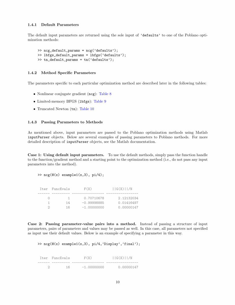
1.4.3 Passing Parameters to Methods

As mentioned above, input parameters are passed to the Poblano optimization methods using MatlabinputParser objects. Below are several examples of passing parameters to Poblano methods. For moredetailed description of inputParser objects, see the Matlab documentation.

Case 1: Using default input parameters. To use the default methods, simply pass the function handleto the function/gradient method and a starting point to the optimization method (i.e., do not pass any inputparameters into the method).

>> ncg(@(x) example1(x,3), pi/4);


0 1 0.70710678 2.121320341 14 -0.99998885 0.014164972 16 -1.00000000 0.00000147

Case 2: Passing parameter-value pairs into a method. Instead of passing a structure of inputparameters, pairs of parameters and values may be passed as well. In this case, all parameters not specifiedas input use their default values. Below is an example of specifying a parameter in this way.

>> ncg(@(x) example1(x,3), pi/4,’Display’,’final’);


2 16 -1.00000000 0.00000147

10

Case 3: Passing input parameters as fields in a structure. Input parameters can be passed as fieldsin a structure. Note, though, that since each optimization method uses method specific parameters, it issuggested to start from a structure of the default parameters for a particular method. Once the structure ofdefault parameters has been created, the individual parameters (i.e., fields in the structure) can be changed.Below is an example of this for the ncg method.

>> params = ncg(’defaults’);>> params.MaxIters = 1;>> ncg(@(x) example1(x,3), pi/4, params);


0 1 0.70710678 2.121320341 14 -0.99998885 0.01416497

Case 4: Using parameters from one run in another run. One of the outputs returned by thePoblano optimization methods is the inputParser object of the input parameters used in that run. Thatobject contains a field called Results, which can be passed as the input parameters to another run. Forexample, this is helpful when running comparisons of methods where only one parameter is changed. Shownbelow is such an example, where default parameters are used in one run, and the same parameters with justa single change are used in another run.

>> out = ncg(@(x) example1(x,3), pi./[4 5 6]’);>> params = out.Params.Results;>> params.Display = ’final’;>> ncg(@(x) example1(x,3), pi./[4 5 6]’, params);


0 1 2.65816330 0.771680961 7 -0.63998759 0.788695702 11 -0.79991790 0.606938193 14 -0.99926100 0.038438274 16 -0.99999997 0.000237395 18 -1.00000000 0.00000000


5 18 -1.00000000 0.00000000

11

1.5 Optimization Output Parameters

Each of the optimization methods in Poblano outputs a single structure containing fields described in Table 5.

Parameter Description TypeX Final iterate vector, doubleF Function value at X doubleG Gradient at X vector, doubleParams Input parameters used for the minimization method (as parsed Matlab

inputParser object)struct

FuncEvals Number of function evaluations performed intIters Number of iterations performed (see individual optimization routines for

details on what each iteration consists of)int

ExitFlag Termination flag, with one of the following values int0 : scaled gradient norm < StopTol input parameter)1 : maximum number of iterations exceeded2 : maximum number of function values exceeded3 : relative change in function value < RelFuncTol input parameter4 : NaNs found in F, G, or ||G||

Table 5: Output parameters returned by all Poblano optimization methods.

1.5.1 Optional Trace Output Parameters

Additional output parameters returned by the Poblano optimization methods are presented in Table 6.The histories (i.e., traces) of different variables and parameters at each iteration are returned as outputparameters if the corresponding input parameters are set to true (see §1.4 for more details on the inputparameters).

Parameter Description TypeTraceX History of X (iterates) matrix, doubleTraceFunc History of the function values of the iterates vector, doubleTraceRelFunc History of the relative difference between the function values at the

current and previous iteratesvector, double

TraceGrad History of the gradients of the iterates matrix, doubleTraceGradNorm History of the norm of the gradients of the iterates vector, doubleTraceFuncEvals History of the number of function evaluations performed at each

iterationvector, int

Table 6: Additional trace output parameters returned by all Poblano optimization methods if requested.

12

1.5.2 Example Output of Optimization Methods

The following example shows the output produced when the default input parameters are used.

>> out = ncg(@(x) example1(x,3), pi/4)


0 1 0.70710678 2.121320341 14 -0.99998885 0.014164972 16 -1.00000000 0.00000147

out =Params: [1x1 inputParser]

ExitFlag: 0X: 70.6858F: -1.0000G: -1.4734e-06

FuncEvals: 16Iters: 2

The following example presents an example where a method terminates before convergence (due to a limiton the number of iterations allowed).

>> out = ncg(@(x) example1(x,3), pi/4, ’Display’, ’final’, ’MaxIters’, 1)


1 14 -0.99998885 0.01416497


ExitFlag: 1X: 70.6843F: -1.0000G: -0.0142


The following shows the ability to save traces of the different information for each iteration.

>> out = ncg(@(x) example1(x,3), rand(3,1),’TraceX’,true,’TraceFunc’,true, ...’TraceRelFunc’,true,’TraceGrad’,true,’TraceGradNorm’,true,’TraceFuncEvals’,true)


0 1 0.92763793 1.637364131 5 -2.71395809 0.72556878

13

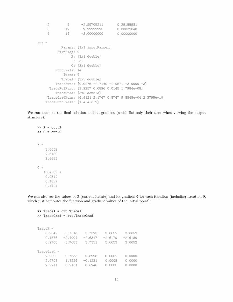
2 9 -2.95705211 0.291559813 12 -2.99999995 0.000328484 14 -3.00000000 0.00000000


ExitFlag: 0X: [3x1 double]F: -3G: [3x1 double]

FuncEvals: 14Iters: 4TraceX: [3x5 double]

TraceFunc: [0.9276 -2.7140 -2.9571 -3.0000 -3]TraceRelFunc: [3.9257 0.0896 0.0145 1.7984e-08]

TraceGrad: [3x5 double]TraceGradNorm: [4.9121 2.1767 0.8747 9.8545e-04 2.3795e-10]TraceFuncEvals: [1 4 4 3 2]

We can examine the final solution and its gradient (which list only their sizes when viewing the outputstructure):

>> X = out.X>> G = out.G

X =3.6652-2.61803.6652

G =1.0e-09 *0.05120.18390.1421

We can also see the values of X (current iterate) and its gradient G for each iteration (including iteration 0,which just computes the function and gradient values of the initial point):

>> TraceX = out.TraceX>> TraceGrad = out.TraceGrad

TraceX =0.9649 3.7510 3.7323 3.6652 3.66520.1576 -2.4004 -2.6317 -2.6179 -2.61800.9706 3.7683 3.7351 3.6653 3.6652

TraceGrad =-2.9090 0.7635 0.5998 0.0002 0.00002.6708 1.8224 -0.1231 0.0008 0.0000-2.9211 0.9131 0.6246 0.0006 0.0000

14

1.6 Examples of Running Poblano Optimizers

To solve a problem using Poblano, the following steps are performed:

• Step 1: Create M-file for objective and gradient. An M-file which takes a vector as input andprovides a scalar function value and gradient vector (the same size as the input) must be provided tothe Poblano optimizers.

• Step 2: Call the optimizer. One of the Poblano optimizers is called, taking an anonymous functionhandle to the function to be minimized, a starting point, and an optional set of optimizer parametersas inputs.

The following examples of functions are provided with Poblano.

1.6.1 Example 1: Multivariate Sum

The following example is a simple multivariate function, f1 : RN → R, that can be minimized using Poblano:

f1(x) =N∑

n=1

sin(axi)

(∇f1(x))i = a cos(axi) , i = 1, . . . , N

where a is a scalar parameter.

Listed below are the contents of the example1.m M-file distributed with the Poblano code. This is anexample of a self-contained function requiring a vector of independent variables and an optional scalar inputparameter for a.

function [f,g]=example1(x,a)if nargin < 2, a = 1; endf = sum(sin(a*x));g = a*cos(a*x);

The following presents a call to the ncg optimizer using the default parameters (see §2.1 for more details)along with the output of Poblano. By default, at each iteration Poblano displays the number of functionevaluations (FuncEvals), the function value at the current iterate (F(X)), and the Euclidean norm of thescaled gradient at the current iterate (||G(X)||/N, where N is the size of X) for each iteration. The output ofPoblano optimizers is a Matlab structure containing the solution. The structure of the output is describedin detail in §1.5.

>> out = ncg(@(x) example1(x,3), pi/4)


0 1 0.70710678 2.121320341 14 -0.99998885 0.014164972 16 -1.00000000 0.00000147

15


ExitFlag: 0X: 70.6858F: -1.0000G: -1.4734e-06


1.6.2 Example 2: Matrix Decomposition

The following example is a more complicated function involving matrix variables. As the Poblano methodsrequire scalar functions with vector inputs, variable matrices must be reshaped into vectors first. Theproblem in this example is to find a rank-k decomposition, UV T, of a m×n matrix, A, which minimizes theFrobenius norm of the fit of the decomposition to the matrix. More formally,

f2 =12‖A− UV T‖2F

∇Uf2 = −(A− UV T)V

∇V f2 = −(A− UV T)TU

where A ∈ Rm×n is a matrix with rank ≥ k, U ∈ Rm×k, and V ∈ Rn×k. This problem can be solved usingPoblano by providing an M-file that computes the function and gradient shown above but that takes U andV as input in vectorized form.

Listed below are the contents of the example2.m M-file distributed with the Poblano code. Note that theinput Data is required and is a structure containing the matrix to be decomposed, A, and the desired rank,k. This example also illustrates how the vectorized form of the factor matrices, U and V , are converted tomatrix form for the function and gradient computations.

function [f,g]=example2(x,Data)% Data setup[m,n] = size(Data.A);k = Data.rank;U = reshape(x(1:m*k),m,k);V = reshape(x(m*k+1:m*k+n*k),n,k);

% Function value (residual)AmUVt = Data.A-U*V’;f = 0.5*norm(AmUVt,’fro’)^2;

% First derivatives computed in matrix formg = zeros((m+n)*k,1);g(1:m*k) = -reshape(AmUVt*V,m*k,1);g(m*k+1:end) = -reshape(AmUVt’*U,n*k,1);

Included with Poblano are two helper functions and which can be used to generate problems instancesalong with starting points (example2 init.m) and extract the factors U and V from a solution vector(example2 extract.m). We show an example of their use below.

16

>> randn(’state’,0);>> m = 4; n = 3; k = 2;>> [x0,Data] = example2_init(m,n,k)>> out = ncg(@(x) example2(x,Data), x0, ’RelFuncTol’, 1e-16, ’StopTol’, 1e-8, ...

’MaxFuncEvals’,1000,’Display’,’final’)

x0 =-0.588316543014189

2.1831858181971-0.1363958830865960.113931313520811.06676821135919

0.0592814605236053-0.095648405483669-0.8323494636500220.29441081639264-1.33618185793780.7143245518189521.62356206444627

-0.6917757017022870.857996672828263

Data =rank: 2

A: [4x3 double]


29 67 0.28420491 0.00000001


ExitFlag: 0X: [14x1 double]F: 0.284204907556308G: [14x1 double]


17

Extracting the factors from the solution, we see that we have found a solution, since the the Euclidean normof the difference between the matrix and the approximate solution is equal to the the k+ 1 singular value ofA [4, Theorem 2.5.3].

>> [U,V] = example2_extract(4,3,2,out.X);>> norm_diff = norm(Data.A-U*V’)>> sv = svd(Data.A);>> sv_k_plus_1 = sv(k+1)

norm_diff =0.753929582330216

sv_k_plus_1 =0.753929582330215

18

2 Optimization Methods

2.1 Nonlinear Conjugate Gradient

Nonlinear conjugate gradient (NCG) methods [9] are used to solve unconstrained nonlinear optimizationproblems. They are extensions of the conjugate gradient iterative method for solving linear systems adaptedto solve unconstrained nonlinear optimization problems.

The Poblano function for the nonlinear conjugate gradient methods is called ncg.

2.1.1 Method Description

The general steps of NCG methods are given below in high-level pseudo-code:

1. Input: x0, a starting point2. Evaluate f0 = f(x0), g0 = ∇f(x0)3. Set p0 = −g0, i = 04. while ‖gi‖ > 05. Compute a step length αi and set xi+1 = xi + αipi

6. Set gi = ∇f(xi+1)7. Compute βi+1

8. Set pi+1 = −gi+1 + βi+1pi

9. Set i = i+ 110. end while11. Output: xi ≈ x∗

Conjugate direction updates. The computation of βi+1 in Step 7 above leads to different NCG methods.The update methods for βi+1 available in Poblano are listed in Table 7. Note that the special case of βi+1 = 0leads to the steepest descent method [9], which is available in Poblano by specifying this update using theinput parameter described in Table 8.

Update Type Update Formula

Fletcher-Reeves [3] βi+1 =gT

i+1−gi+1

gTi gi

Polak-Ribiere [12] βi+1 =gT

i+1(gi+1−gi)gT

i gi

Hestenes-Stiefel [5] βi+1 =gT

i+1(gi+1−gi)pT

i (gi+1−gi)

Table 7: Conjugate direction updates available in Poblano.

Negative update coefficients. In cases where the update coefficient is negative, i.e., βi+1 < 0, it is setto 0 to avoid directions that are not descent directions [9].

19

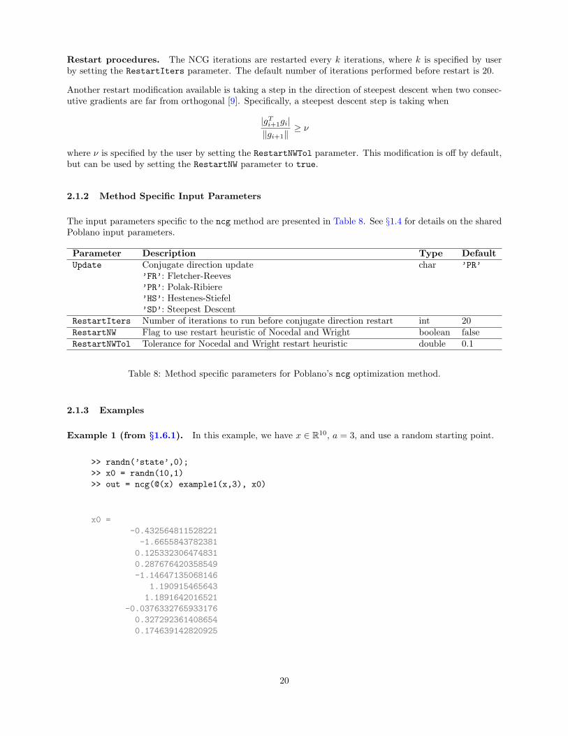
Restart procedures. The NCG iterations are restarted every k iterations, where k is specified by userby setting the RestartIters parameter. The default number of iterations performed before restart is 20.

Another restart modification available is taking a step in the direction of steepest descent when two consec-utive gradients are far from orthogonal [9]. Specifically, a steepest descent step is taking when

|gTi+1gi|‖gi+1‖

≥ ν

where ν is specified by the user by setting the RestartNWTol parameter. This modification is off by default,but can be used by setting the RestartNW parameter to true.

2.1.2 Method Specific Input Parameters

The input parameters specific to the ncg method are presented in Table 8. See §1.4 for details on the sharedPoblano input parameters.

Parameter Description Type DefaultUpdate Conjugate direction update char ’PR’

’FR’: Fletcher-Reeves’PR’: Polak-Ribiere’HS’: Hestenes-Stiefel’SD’: Steepest Descent

RestartIters Number of iterations to run before conjugate direction restart int 20RestartNW Flag to use restart heuristic of Nocedal and Wright boolean falseRestartNWTol Tolerance for Nocedal and Wright restart heuristic double 0.1

Table 8: Method specific parameters for Poblano’s ncg optimization method.

2.1.3 Examples

Example 1 (from §1.6.1). In this example, we have x ∈ R10, a = 3, and use a random starting point.

>> randn(’state’,0);>> x0 = randn(10,1)>> out = ncg(@(x) example1(x,3), x0)

x0 =-0.432564811528221-1.66558437823810.1253323064748310.287676420358549-1.14647135068146

1.1909154656431.1891642016521

-0.03763327659331760.3272923614086540.174639142820925

20


0 1 1.80545257 0.738111141 5 -4.10636797 0.545641692 8 -5.76811976 0.520396183 12 -7.62995880 0.254438874 15 -8.01672533 0.063290925 20 -9.51983614 0.285717596 25 -9.54169917 0.278200837 28 -9.99984082 0.005352718 30 -10.00000000 0.00000221


ExitFlag: 0X: [10x1 double]F: -9.99999999997292G: [10x1 double]


Example 2 (from §1.6.2). In this example, we compute a rank-4 approximation to a 4×4 Pascal matrix(generated using the Matlab function pascal(4)). The starting point is random vector. Note that in theinterest of space, Poblano is set to display only the final iteration is this example.

>> m = 4; n = 4; k = 4;>> Data.rank = k;>> Data.A = pascal(m);>> randn(’state’,0);>> x0 = randn((m+n)*k,1);>> out = ncg(@(x) example2(x,Data), x0, ’Display’, ’final’)


39 101 0.00005424 0.00136338


ExitFlag: 2X: [32x1 double]F: 5.42435362453638e-05G: [32x1 double]


The fact that out.ExitFlag>0 indicates that the method did not converge to the specified tolerance (i.e.,the default StopTol input parameter value of 10−5). From Table 5, we see that this exit flag indicates thatthe maximum number of function evaluations was exceeded. Increasing the number of maximum numbersof function evaluations and iterations allowed, the optimizer converges to a solution within the specifiedtolerance.

21

>> out = ncg(@(x) example2(x,Data), x0, ’MaxIters’,1000, ...’MaxFuncEvals’,10000,’Display’,’final’)


76 175 0.00000002 0.00000683




Verifying the solution, we see that we find a matrix decomposition which fits the matrix with very smallrelative error (given the stopping tolerance of 10−5 used by the optimizer).

>> [U,V] = example2_extract(m,n,k,out.X);>> norm(Data.A-U*V’)/norm(Data.A)

ans =5.48283898063955e-06

22

2.2 Limited-memory BFGS

Limited-memory quasi-Newton methods [9] are a class of methods that compute and/or maintain simple,compact approximations of the Hessian matrices of second derivatives, which are used determining searchdirections. Poblano includes the limited-memory BFGS (L-BFGS) method, a variant of these methods whoseHessian approximations are based on the BFGS method (see [2] for more details).

The Poblano function for the L-BFGS method is called lbfgs.


The general steps of L-BFGS methods are given below in high-level pseudo-code [9]:

1. Input: x0, a starting point; M > 0, an integer2. Evaluate f0 = f(x0), g0 = ∇f(x0)3. Set p0 = −g0, γ0 = 1, i = 04. while ‖gi‖ > 05. Choose an initial Hessian approximation: H0

i = γiI6. Compute a step direction pi = −r using TwoLoopRecursion method7. Compute a step length αi and set xi+1 = xi + αipi

8. Set gi = ∇f(xi+1)9. if i > M10. Discard vectors {si−m, yi−m} from storage11. end if12. Set and store si = xi+1 − xi and yi = gi+1 − gi

13. Set i = i+ 114. end while15. Output: xi ≈ x∗

Computing the step direction. In Step 6 in the above method, the computation of the step directionis performed using the following method (assume we are at iteration i) [9]:

TwoLoopRecursion1. q = gi

2. for k = i− 1, i− 2, . . . , i−m3. ak = (sT

k q)/(yTk sk)

4. q = q − akyk

5. end for6. r = H0

i q7. for k = i−m, i−m+ 1, . . . , i− 18. b = (yT

k r)/(yTk sk)

9. r = r + (ak − b)sk

10. end for11. Output: r = Higi


The input parameters specific to the lbfgs method are presented in Table 9. See §1.4 for details on theshared Poblano input parameters.

23

Parameter Description Type DefaultM Limited memory parameter (i.e., number of vectors s and y to store

from previous iterations)int 5

Table 9: Method specific parameters for Poblano’s lbfgs optimization method.

2.2.3 Examples

Below are the results of using the lbfgs method in Poblano to solve example problems solved using the ncgmethod in §2.1.3. Note the different methods leads to slightly different solutions and a different number offunction evaluations.

Example 1. In this example, we have x ∈ R10 and a = 3, and use a random starting point.

>> randn(’state’,0);>> x0 = randn(10,1)>> out = lbfgs(@(x) example1(x,3), x0)

x0 =-0.432564811528221-1.66558437823810.1253323064748310.287676420358549-1.14647135068146

1.1909154656431.1891642016521

-0.03763327659331760.3272923614086540.174639142820925


0 1 1.80545257 0.738111141 5 -4.10636797 0.545641692 9 -5.78542020 0.518847773 12 -6.92220212 0.415453404 15 -7.59202813 0.297102315 18 -7.95865922 0.259900996 21 -8.18606788 0.224571337 24 -9.21285389 0.354684228 27 -9.68427296 0.232331429 30 -9.83727919 0.1693695810 32 -9.91014546 0.1261921211 35 -9.94394171 0.1001207512 37 -9.96737038 0.0764545413 39 -9.99998661 0.0015526414 40 -10.00000000 0.0000273915 42 -10.00000000 0.00000010

24


ExitFlag: 0X: [10x1 double]F: -9.99999999999995G: [10x1 double]


Example 2. In this example, we compute a rank 2 approximation to a 4 × 4 Pascal matrix (generatedusing the Matlab function pascal(4)). The starting point is a random vector.

>> m = 4; n = 4; k = 4;>> Data.rank = k;>> Data.A = pascal(m);>> randn(’state’,0);>> x0 = randn((m+n)*k,1);>> out = lbfgs(@(x) example2(x,Data), x0, ’Display’, ’final’)


46 100 0.00000584 0.00032464




As for the ncg method, the fact that out.ExitFlag>0 indicates that the method did not converge tothe specified tolerance (i.e., the default StopTol input parameter value of 10−5). Since the maximumnumber of function evaluations was exceeded, we can increasing the number of maximum numbers of functionevaluations and iterations allowed, and the optimizer converges to a solution within the specified tolerance.

>> out = lbfgs(@(x) example2(x,Data), x0, ’MaxIters’,1000, ...’MaxFuncEvals’,10000,’Display’,’final’)


67 143 0.00000000 0.00000602

25






ans =2.54707192131722e-06

For Example 2, we see that lbfgs requires slightly fewer function evaluations than ncg to solve the problem(143 versus 175). Performance of the different methods in Poblano is dependent on both the method andthe particular parameters chosen. Thus, it is recommended that several test runs on smaller problems areperformed initially using the different methods to help decide which method and set of parameters worksbest for a particular class of problems.

26

2.3 Truncated Newton

Truncated Newton (TN) methods for minimization are Newton methods in which the Newton direction isonly approximated at each iteration (thus reducing computation). Furthermore, the Poblano implementationof the truncated Newton method does not require an explicit Hessian matrix in the computation of theapproximate Newton direction (thus reducing storage requirements).

The Poblano function for the truncated Newton method is called tn.


The general steps of the TN method in Poblano is given below in high-level pseudo-code [1]:

1. Input: x0, a starting point; N > 0, an integer; η02. Evaluate f0 = f(x0), g0 = ∇f(x0)3. Set i = 04. while ‖gi‖ > 05. Compute the conjugate gradient stopping tolerance, ηi

6. Compute pi by solving ∇2f(xi)p = −gi using a linear conjugate gradient (CG) method7. Compute a step length αi and set xi+1 = xi + αipi

8. Set gi = ∇f(xi+1)9. Set i = i+ 110. end while11. Output: xi ≈ x∗

Notes

• In Step 5, the linear conjugate gradient (CG) method stopping tolerance is allowed to change at eachiteration. The input parameter CGTolType determines how ηi is computed.

• In Step 6

– One of Matlab’s CG methods is used to solve for pi: symmlq (designed for symmetric indefinitesystems) or pcg (the classical CG method for symmetric positive definite systems). The inputparameter CGSolver controls the choice of CG method to use.

– The maximum number of CG iterations, N , is specified using the input parameter CGIters.

– The CG method stops when ‖ − gi −∇2f(xi)pi‖ ≤ ηi‖gi‖ .

– In the CG method, matrix-vector products involving ∇2f(xi) times a vector v are approximatedusing the following finite difference approximation [1]:

∇2f(xi)v ≈∇f(xi + σv)−∇f(xi)

σ

The difference step, σ, is specified using the input parameter HessVecFDStep. The computationof the finite difference approximation is performed using the hessvec fd provided with Poblano.

27


The input parameters specific to the tn method are presented in Table 10. See §1.4 for details on the sharedPoblano input parameters.

Parameter Description Type DefaultCGIters Maximum number of conjugate gradient iterations allowed int 5CGTolType CG stopping tolerance type used char ’quadratic’

’quadratic’: ‖R‖/‖G‖ < min(0.5, ‖G‖)’superlinear’: ‖R‖/‖G‖ < min(0.5,

√‖G‖)

’fixed’: ‖R‖ < CGTolR is the residual and G is the gradient

CGTol CG stopping tolerance when CGTolType is ’fixed’ double 1e-6HessVecFDStep Hessian vector product finite difference step double 10−10

0 : Use iterate-based step: 10−8(1 + ‖X‖2)> 0 : Fixed value to use at the difference step

CGSolver Matlab CG method used to solve for search direction string ’symmlq’’symmlq’: symmetric LQ method [11]’pcg’: classical CG method [5]

Table 10: Method specific parameters for Poblano’s tn optimization method.

2.3.3 Examples

Below are the results of using the tn method in Poblano to solve example problems solved using the ncgmethod in §2.1.3 and lbfgs method in §2.2.3.

Example 1. In this example, we have x ∈ R10 and a = 3, and use a random starting point.

>> randn(’state’,0);>> x0 = randn(10,1)>> out = tn(@(x) example1(x,3), x0)

x0 =-0.432564811528221-1.66558437823810.1253323064748310.287676420358549-1.14647135068146

1.1909154656431.1891642016521

-0.03763327659331760.3272923614086540.174639142820925

28


0 1 1.80545257 0.73811114tn: line search warning = 0

1 10 -4.10636797 0.545641692 18 -4.21263331 0.41893997

tn: line search warning = 03 28 -7.18352472 0.365475464 34 -8.07095085 0.11618518

tn: line search warning = 05 41 -9.87251163 0.150574766 46 -9.99999862 0.000497537 50 -10.00000000 0.00000000


ExitFlag: 0X: [10x1 double]F: -10G: [10x1 double]


Note that in this example the More-Thuente line search in tn method displays a warning during iterations1, 3 and 5, indicating that the norm of the search direction is nearly 0. In those cases, the steepest descentdirection is used for the search direction during those iterations.

Example 2. In this example, we compute a rank 2 approximation to a 4 × 4 Pascal matrix (generatedusing the Matlab function pascal(4)). The starting point is a random vector.

>> m = 4; n = 4; k = 4;>> Data.rank = k;>> Data.A = pascal(m);>> randn(’state’,0);>> x0 = randn((m+n)*k,1);>> out = tn(@(x) example2(x,Data), x0, ’Display’, ’final’)


16 105 0.00013951 0.00060739




29

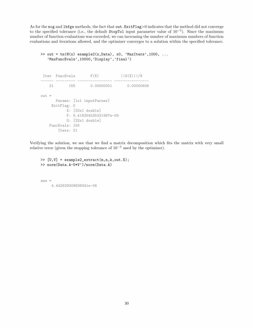
As for the ncg and lbfgs methods, the fact that out.ExitFlag>0 indicates that the method did not convergeto the specified tolerance (i.e., the default StopTol input parameter value of 10−5). Since the maximumnumber of function evaluations was exceeded, we can increasing the number of maximum numbers of functionevaluations and iterations allowed, and the optimizer converges to a solution within the specified tolerance.

>> out = tn(@(x) example2(x,Data), x0, ’MaxIters’,1000, ...’MaxFuncEvals’,10000,’Display’,’final’)


21 155 0.00000001 0.00000606






ans =4.442629309639341e-06

30

3 Checking Gradient Calculations

Analytic gradients can be checked using finite difference approximations. The Poblano functiongradientcheck computes the gradient approximations and compares the results to the analytic gradientusing a user-supplied objective function/gradient M-file. The user can choose one of several difference for-mulas as well as the difference step used in the computations.

3.1 Difference Formulas

The difference formulas for approximating the gradients in Poblano are listed in Table 11. For more detailson the different formulas, see [9].

Formula Type Formula

Forward Differences∂f

∂xi(x) ≈ f(x+ hei)− f(x)

h

Backward Differences∂f

∂xi(x) ≈ f(x)− f(x− hei)

h

Centered Differences∂f

∂xi(x) ≈ f(x+ hei)− f(x− hei)

2h

Note: ei is a vector the same size as x with a 1 in element i and zeros elsewhere,

and h is a user-defined parameter.

Table 11: Difference formulas available in Poblano for checking user-defined gradients.

The type of finite differences to use is specified using the DifferenceType input parameter, and the valueof h is specified using the DifferenceStep input parameter. For a detailed discussion on the impact of thechoice of h on the quality of the approximation, see [10].

3.2 Gradient Check Input Parameters

The input parameters available for the gradientcheck function are presented in Table 12.

Parameter Description Type DefaultDifferenceType Difference formula to use char ’forward’

’forward’: gi = (f(x+ hei)− f(x))/h’backward’: gi = (f(x)− f(x− hei))/h’centered’: gi = (f(x+ hei)− f(x− hei))/(2h)

DifferenceStep Value of h in difference formulae double 10−8

Table 12: Input parameters for Poblano’s gradientcheck function.

31

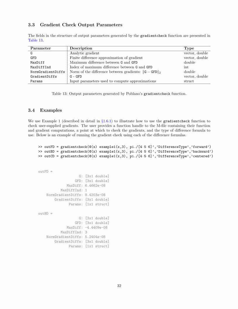
3.3 Gradient Check Output Parameters

The fields in the structure of output parameters generated by the gradientcheck function are presented inTable 13.

Parameter Description TypeG Analytic gradient vector, doubleGFD Finite difference approximation of gradient vector, doubleMaxDiff Maximum difference between G and GFD doubleMaxDiffInd Index of maximum difference between G and GFD intNormGradientDiffs Norm of the difference between gradients: ‖G− GFD‖2 doubleGradientDiffs G - GFD vector, doubleParams Input parameters used to compute approximations struct

Table 13: Output parameters generated by Poblano’s gradientcheck function.

3.4 Examples

We use Example 1 (described in detail in §1.6.1) to illustrate how to use the gradientcheck function tocheck user-supplied gradients. The user provides a function handle to the M-file containing their functionand gradient computations, a point at which to check the gradients, and the type of difference formula touse. Below is an example of running the gradient check using each of the difference formulas.

>> outFD = gradientcheck(@(x) example1(x,3), pi./[4 5 6]’,’DifferenceType’,’forward’)>> outBD = gradientcheck(@(x) example1(x,3), pi./[4 5 6]’,’DifferenceType’,’backward’)>> outCD = gradientcheck(@(x) example1(x,3), pi./[4 5 6]’,’DifferenceType’,’centered’)

outFD =G: [3x1 double]

GFD: [3x1 double]MaxDiff: 6.4662e-08

MaxDiffInd: 1NormGradientDiffs: 8.4203e-08

GradientDiffs: [3x1 double]Params: [1x1 struct]

outBD =G: [3x1 double]

GFD: [3x1 double]MaxDiff: -4.4409e-08



32

outCD =G: [3x1 double]

GFD: [3x1 double]MaxDiff: 2.0253e-08



Note the different gradients produced using the various differencing formulas:

>> format long>> [outFD.G outFD.GFD outBD.GFD outCD.GFD]

ans =-2.121320343559642 -2.121320408221550 -2.121320319403708 -2.121320363812629-0.927050983124842 -0.927051013732694 -0.927050969323773 -0.9270509915282330.000000000000000 -0.000000044408921 0.000000044408921 0

33

This page intentionally left blank.

34

4 Numerical Experiments

To demonstrate the performance of the Poblano methods, we present results of runs of the different methodsin this section. All experiments were performed using Matlab 7.9 on a Linux Workstation (RedHat 5.2) with2 Quad-Core Intel Xeon 3.0GHz processors and 32GB RAM.

4.1 Description of Test Problems

The test problems used in the experiments presented here are from the More, Garbow, and Hillstromcollection, which is described in detail in [7]. The Matlab code used for these problems is provided as partof the SolvOpt optimization software [6], available at http://www.kfunigraz.ac.at/imawww/kuntsevich/solvopt/. There are 34 test problems in this collection.

4.2 Results

Results in this section are for optimization runs using the default parameters, with the exception of the stop-ping criteria parameters, which were changed to allow more computation and find more accurate solutions.The parameters changed from their default values are as follows:

params.Display = ’off’params.MaxIters = 20000;params.MaxFuncEvals = 50000;params.RelFuncTol = 1e-16;params.StopTol = 1e-12;

For all of the results presented in this section, the function value computed by the Poblano methods isdenoted by F ∗, the solution is denoted by F ∗, and the error is |F ∗ − F ∗|/max{1, |F ∗|}. The “solutions”are those reported as having the lowest function values throughout the literature. A survey of the problemcharacteristics, along with known local optimizers can be found on the SolvOpt web site (http://www.kfunigraz.ac.at/imawww/kuntsevich/solvopt/results.html).

For this test collection, we say the problem is solved if the error as defined above is less than 10−8. We seethat the Poblano methods solve most of the problems using the default input parameters, but have difficultywith a few that require particular parameter settings. Specifically, the initial step size in the line searchmethod appears to be the most sensitive parameter across all of the methods. More investigation into theeffective use of this parameter for other problem classes is planned for future work. Below are more detailsof the results for the different Poblano methods.

4.2.1 Nonlinear Conjugate Gradient Methods

The results of the tests for the ncg method using Polak-Ribiere (PR) conjugate direction updates are pre-sented in Table 14. Note that several problems (3, 6, 10, 11, 17, 20, 27 and 31) were not solved using theparameters listed above. With more testing, specifically with different values of the initial step size used inthe line search (specified using the LineSearch initialstep parameter) and the number of iterations toperform before restarting the conjugate directions using a step in the steepest direction (specified using theRestartIters parameter), solutions to all problems except #10 were found. Table 15 presents parameterchoices leading to successful runs of the ncg method using PR conjugate direction updates.

The results of the tests for the ncg method using Hestenes-Stiefel (HS) conjugate direction updates arepresented in Table 16. Again, several problems (3, 6, 10, 11 and 31) were not solved using the parameters

35

http://www.kfunigraz.ac.at/imawww/kuntsevich/solvopt/


http://www.kfunigraz.ac.at/imawww/kuntsevich/solvopt/results.html

http://www.kfunigraz.ac.at/imawww/kuntsevich/solvopt/results.html

listed above. Table 17 presents parameter choices leading to successful runs of the ncg method using HSconjugate direction updates. Note that we did not find parameters to solve problem #10 with this methodeither.

Finally, the results of the tests for the ncg method using Fletcher-Reeves (FR) conjugate direction updatesare presented in Table 18. We see that even more problems (3, 6, 10, 11, 17, 18, 20 and 31) were not solvedusing the parameters listed above. Table 19 presents parameter choices leading to successful runs of the ncgmethod using FR conjugate direction updates. Note that we did not find parameters to solve problem #10with this method either.

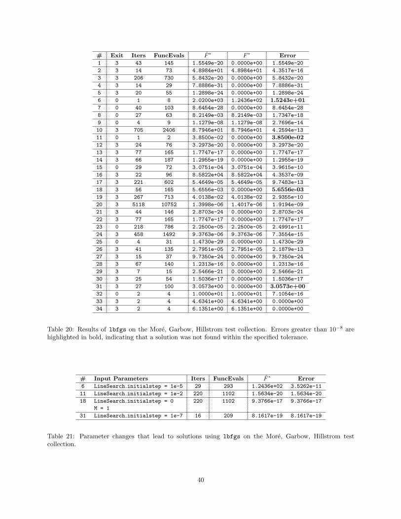
4.2.2 Limited Memory BFGS Method

The results of the tests for the lbfgs method are presented in Table 20. Compared to the ncg methods,fewer problems (3, 6 and 31) were not solved using the parameters listed above with the lbfgs method.Most notably, lbfgs was able to solve problem #10, illustrating that some problems are better suited to thedifferent Poblano methods. With more testing, specifically with different values of the initial step size usedin the line search (specified using the LineSearch initialstep parameter), solutions to all problems werefound. Table 21 presents parameter choices leading to successful runs of the lbfgs method.

4.2.3 Truncated Newton Method

The results of the tests for the tn method are presented in Table 22. Note that several problems (10, 11, 20and 31) were not solved using this method. However, problem #6 was solved (which was not solved usingany of the other Poblano methods), again illustrating that some problems are better suited to tn than theother Poblano methods. With more testing, specifically with different values of the initial step size usedin the line search (specified using the LineSearch initialstep parameter), solutions to all problems werefound, with the exception of problem #10. Table 23 presents parameter choices leading to successful runsof the tn method.

36

# Exit Iters FuncEvals F ∗ F ∗ Error

1 3 20 90 1.3972e-18 0.0000e+00 1.3972e-18

2 3 11 71 4.8984e+01 4.8984e+01 5.8022e-16

3 3 3343 39373 6.3684e-07 0.0000e+00 6.3684e-07

4 3 14 126 1.4092e-21 0.0000e+00 1.4092e-21

5 3 12 39 1.7216e-17 0.0000e+00 1.7216e-17

6 0 1 8 2.0200e+03 1.2436e+02 1.5243e+01

7 3 53 158 5.2506e-18 0.0000e+00 5.2506e-18

8 3 28 108 8.2149e-03 8.2149e-03 1.2143e-17

9 0 5 14 1.1279e-08 1.1279e-08 2.7696e-14

10 3 262 1232 9.5458e+04 8.7946e+01 1.0844e+03

11 0 1 2 3.8500e-02 0.0000e+00 3.8500e-02

12 0 15 62 3.9189e-32 0.0000e+00 3.9189e-32

13 3 129 352 1.5737e-16 0.0000e+00 1.5737e-16

14 3 47 155 2.7220e-18 0.0000e+00 2.7220e-18

15 3 58 165 3.0751e-04 3.0751e-04 3.9615e-10

16 3 34 168 8.5822e+04 8.5822e+04 4.3537e-09

17 3 3122 7970 5.5227e-05 5.4649e-05 5.7842e-07

18 3 1181 2938 2.1947e-16 0.0000e+00 2.1947e-16

19 3 381 876 4.0138e-02 4.0138e-02 2.9355e-10

20 3 14842 30157 1.4233e-06 1.4017e-06 2.1546e-08

21 3 20 90 6.9775e-18 0.0000e+00 6.9775e-18

22 3 129 352 1.5737e-16 0.0000e+00 1.5737e-16

23 0 90 415 2.2500e-05 2.2500e-05 2.4991e-11

24 3 142 520 9.3763e-06 9.3763e-06 7.4196e-15

25 3 5 27 7.4647e-25 0.0000e+00 7.4647e-25

26 3 47 144 2.7951e-05 2.7951e-05 2.1878e-13

27 3 2 8 8.2202e-03 0.0000e+00 8.2202e-03

28 3 79 160 1.4117e-17 0.0000e+00 1.4117e-17

29 3 7 16 9.1648e-19 0.0000e+00 9.1648e-19

30 3 30 75 1.0410e-17 0.0000e+00 1.0410e-17

31 3 41 97 3.0573e+00 0.0000e+00 3.0573e+00

32 0 2 5 1.0000e+01 1.0000e+01 0.0000e+00

33 3 2 5 4.6341e+00 4.6341e+00 0.0000e+00

34 3 2 5 6.1351e+00 6.1351e+00 0.0000e+00

Table 14: Results of ncg using PR updates on the More, Garbow, Hillstrom test collection. Errors greaterthan 10−8 are highlighted in bold, indicating that a solution was not found within the specified tolerance.

# Input Parameters Iters FuncEvals F ∗ Error

3 LineSearch initialstep = 1e-5 19 152 9.9821e-09 9.9821e-09

RestartIters = 40

6 LineSearch initialstep = 1e-5 19 125 1.2436e+02 3.5262e-11

RestartIters = 40


RestartIters = 40



RestartIters = 50

27 LineSearch initialstep = 0.5 11 38 1.3336e-25 1.3336e-25


Table 15: Parameter changes that lead to solutions using ncg with PR updates on the More, Garbow,Hillstrom test collection.

37


1 3 20 89 1.0497e-16 0.0000e+00 1.0497e-16

2 3 10 69 4.8984e+01 4.8984e+01 2.9011e-16

3 2 4329 50001 4.4263e-08 0.0000e+00 4.4263e-08

4 3 9 83 1.3553e-18 0.0000e+00 1.3553e-18

5 3 12 39 4.3127e-19 0.0000e+00 4.3127e-19

6 0 1 8 2.0200e+03 1.2436e+02 1.5243e+01

7 3 27 98 1.8656e-20 0.0000e+00 1.8656e-20

8 3 25 92 8.2149e-03 8.2149e-03 1.2143e-17

9 3 5 31 1.1279e-08 1.1279e-08 2.7696e-14

10 3 49 332 1.0856e+05 8.7946e+01 1.2334e+03

11 0 1 2 3.8500e-02 0.0000e+00 3.8500e-02

12 0 15 63 5.8794e-30 0.0000e+00 5.8794e-30

13 3 84 258 2.7276e-17 0.0000e+00 2.7276e-17

14 3 44 152 3.4926e-24 0.0000e+00 3.4926e-24

15 3 50 165 3.0751e-04 3.0751e-04 3.9615e-10

16 3 39 176 8.5822e+04 8.5822e+04 4.3537e-09

17 3 942 2754 5.4649e-05 5.4649e-05 4.3964e-12

18 3 748 1977 2.7077e-18 0.0000e+00 2.7077e-18

19 3 237 607 4.0138e-02 4.0138e-02 2.9356e-10

20 3 4685 9977 1.3999e-06 1.4017e-06 1.7946e-09

21 0 22 93 6.1630e-32 0.0000e+00 6.1630e-32

22 3 84 258 2.7276e-17 0.0000e+00 2.7276e-17

23 0 83 381 2.2500e-05 2.2500e-05 2.4991e-11

24 3 170 691 9.3763e-06 9.3763e-06 7.3568e-15

25 3 5 47 7.4570e-25 0.0000e+00 7.4570e-25

26 3 43 144 2.7951e-05 2.7951e-05 2.1878e-13

27 3 9 40 2.5738e-20 0.0000e+00 2.5738e-20

28 3 33 70 8.3475e-18 0.0000e+00 8.3475e-18

29 3 7 16 9.1699e-19 0.0000e+00 9.1699e-19

30 3 29 73 3.4886e-18 0.0000e+00 3.4886e-18

31 3 33 117 3.0573e+00 0.0000e+00 3.0573e+00

32 0 2 5 1.0000e+01 1.0000e+01 0.0000e+00

33 3 2 5 4.6341e+00 4.6341e+00 0.0000e+00

34 3 2 5 6.1351e+00 6.1351e+00 0.0000e+00

Table 16: Results of ncg using HS updates on the More, Garbow, Hillstrom test collection. Errors greaterthan 10−8 are highlighted in bold, indicating that a solution was not found within the specified tolerance.



RestartIters = 40



RestartIters = 40


Table 17: Parameter changes that lead to solutions using ncg with HS updates on the More, Garbow,Hillstrom test collection.

38


1 3 41 199 2.4563e-17 0.0000e+00 2.4563e-17

2 3 25 104 4.8984e+01 4.8984e+01 4.3517e-16

3 3 74 538 1.2259e-03 0.0000e+00 1.2259e-03

4 3 40 304 2.9899e-13 0.0000e+00 2.9899e-13

5 3 27 76 4.7847e-17 0.0000e+00 4.7847e-17

6 0 1 8 2.0200e+03 1.2436e+02 1.5243e+01

7 3 48 153 3.5829e-19 0.0000e+00 3.5829e-19

8 3 46 144 8.2149e-03 8.2149e-03 3.4694e-18

9 3 7 72 1.1279e-08 1.1279e-08 2.7696e-14

10 3 388 2098 3.0166e+04 8.7946e+01 3.4201e+02

11 0 1 2 3.8500e-02 0.0000e+00 3.8500e-02

12 3 19 65 2.6163e-18 0.0000e+00 2.6163e-18

13 3 308 720 1.8955e-16 0.0000e+00 1.8955e-16

14 3 53 219 3.0620e-17 0.0000e+00 3.0620e-17

15 3 83 232 3.0751e-04 3.0751e-04 3.9615e-10

16 3 42 206 8.5822e+04 8.5822e+04 4.3537e-09

17 3 522 2020 5.5389e-05 5.4649e-05 7.4046e-07

18 3 278 644 5.6432e-03 0.0000e+00 5.6432e-03

19 3 385 1003 4.0138e-02 4.0138e-02 2.9355e-10

20 3 14391 29061 2.7316e-06 1.4017e-06 1.3298e-06

21 3 41 199 1.2282e-16 0.0000e+00 1.2282e-16

22 3 308 720 1.8955e-16 0.0000e+00 1.8955e-16

23 3 192 783 2.2500e-05 2.2500e-05 2.4991e-11

24 3 1239 4256 9.3763e-06 9.3763e-06 7.3782e-15

25 0 5 29 1.7256e-31 0.0000e+00 1.7256e-31

26 3 60 187 2.7951e-05 2.7951e-05 2.1877e-13

27 3 10 34 1.0518e-16 0.0000e+00 1.0518e-16

28 3 112 226 1.7248e-16 0.0000e+00 1.7248e-16

29 3 7 16 1.9593e-18 0.0000e+00 1.9593e-18

30 3 30 74 1.1877e-17 0.0000e+00 1.1877e-17

31 3 58 166 3.0573e+00 0.0000e+00 3.0573e+00

32 0 2 5 1.0000e+01 1.0000e+01 3.5527e-16

33 3 2 5 4.6341e+00 4.6341e+00 0.0000e+00

34 3 2 5 6.1351e+00 6.1351e+00 0.0000e+00

Table 18: Results of ncg using FR updates on the More, Garbow, Hillstrom test collection. Errors greaterthan 10−8 are highlighted in bold, indicating that a solution was not found within the specified tolerance.



RestartIters = 50



RestartIters = 40


RestartIters = 40



RestartIters = 50


Table 19: Parameter changes that lead to solutions using ncg with FR updates on the More, Garbow,Hillstrom test collection.

39


1 3 43 145 1.5549e-20 0.0000e+00 1.5549e-20

2 3 14 73 4.8984e+01 4.8984e+01 4.3517e-16

3 3 206 730 5.8432e-20 0.0000e+00 5.8432e-20

4 3 14 29 7.8886e-31 0.0000e+00 7.8886e-31

5 3 20 55 1.2898e-24 0.0000e+00 1.2898e-24

6 0 1 8 2.0200e+03 1.2436e+02 1.5243e+01

7 0 40 103 8.6454e-28 0.0000e+00 8.6454e-28

8 0 27 63 8.2149e-03 8.2149e-03 1.7347e-18

9 0 4 9 1.1279e-08 1.1279e-08 2.7696e-14

10 3 705 2406 8.7946e+01 8.7946e+01 4.2594e-13

11 0 1 2 3.8500e-02 0.0000e+00 3.8500e-02

12 3 24 76 3.2973e-20 0.0000e+00 3.2973e-20

13 3 77 165 1.7747e-17 0.0000e+00 1.7747e-17

14 3 66 187 1.2955e-19 0.0000e+00 1.2955e-19

15 0 29 72 3.0751e-04 3.0751e-04 3.9615e-10

16 3 22 96 8.5822e+04 8.5822e+04 4.3537e-09

17 3 221 602 5.4649e-05 5.4649e-05 9.7483e-13

18 3 56 165 5.6556e-03 0.0000e+00 5.6556e-03

19 3 267 713 4.0138e-02 4.0138e-02 2.9355e-10

20 3 5118 10752 1.3998e-06 1.4017e-06 1.9194e-09

21 3 44 146 2.8703e-24 0.0000e+00 2.8703e-24

22 3 77 165 1.7747e-17 0.0000e+00 1.7747e-17

23 0 218 786 2.2500e-05 2.2500e-05 2.4991e-11

24 3 458 1492 9.3763e-06 9.3763e-06 7.3554e-15

25 0 4 31 1.4730e-29 0.0000e+00 1.4730e-29

26 3 41 135 2.7951e-05 2.7951e-05 2.1879e-13

27 3 15 37 9.7350e-24 0.0000e+00 9.7350e-24

28 3 67 140 1.2313e-16 0.0000e+00 1.2313e-16

29 3 7 15 2.5466e-21 0.0000e+00 2.5466e-21

30 3 25 54 1.5036e-17 0.0000e+00 1.5036e-17

31 3 27 100 3.0573e+00 0.0000e+00 3.0573e+00

32 0 2 4 1.0000e+01 1.0000e+01 7.1054e-16

33 3 2 4 4.6341e+00 4.6341e+00 0.0000e+00

34 3 2 4 6.1351e+00 6.1351e+00 0.0000e+00

Table 20: Results of lbfgs on the More, Garbow, Hillstrom test collection. Errors greater than 10−8 arehighlighted in bold, indicating that a solution was not found within the specified tolerance.




18 LineSearch initialstep = 0 220 1102 9.3766e-17 9.3766e-17

M = 1


Table 21: Parameter changes that lead to solutions using lbfgs on the More, Garbow, Hillstrom testcollection.

40


1 0 105 694 4.9427e-30 0.0000e+00 4.9427e-30

2 3 9 107 4.8984e+01 4.8984e+01 2.9011e-16

3 3 457 3607 3.1474e-09 0.0000e+00 3.1474e-09

4 0 6 36 0.0000e+00 0.0000e+00 0.0000e+00

5 0 13 96 4.4373e-31 0.0000e+00 4.4373e-31

6 3 13 133 1.2436e+02 1.2436e+02 3.5262e-11

7 0 39 245 6.9237e-46 0.0000e+00 6.9237e-46

8 0 9 80 8.2149e-03 8.2149e-03 8.6736e-18

9 0 3 28 1.1279e-08 1.1279e-08 2.7696e-14

10 2 6531 50003 1.1104e+05 8.7946e+01 1.2616e+03

11 0 1 5 3.8500e-02 0.0000e+00 3.8500e-02

12 0 9 74 1.8615e-28 0.0000e+00 1.8615e-28

13 0 25 241 2.3427e-29 0.0000e+00 2.3427e-29

14 0 36 263 1.0481e-26 0.0000e+00 1.0481e-26

15 0 449 4967 3.0751e-04 3.0751e-04 3.9615e-10

16 3 28 237 8.5822e+04 8.5822e+04 4.3537e-09

17 3 2904 30801 5.4649e-05 5.4649e-05 3.3347e-10

18 3 2622 28977 6.3011e-17 0.0000e+00 6.3011e-17

19 3 526 5671 4.0138e-02 4.0138e-02 2.9355e-10

20 2 4654 50006 6.0164e-06 1.4017e-06 4.6147e-06

21 0 96 638 3.9542e-28 0.0000e+00 3.9542e-28

22 0 25 241 2.3427e-29 0.0000e+00 2.3427e-29

23 0 17 207 2.2500e-05 2.2500e-05 2.4991e-11

24 0 63 827 9.3763e-06 9.3763e-06 7.3554e-15

25 0 3 19 2.3419e-31 0.0000e+00 2.3419e-31

26 3 18 249 2.7951e-05 2.7951e-05 2.1878e-13

27 0 6 53 2.7820e-29 0.0000e+00 2.7820e-29

28 3 82 882 1.9402e-17 0.0000e+00 1.9402e-17

29 0 4 33 9.6537e-32 0.0000e+00 9.6537e-32

30 3 16 104 3.4389e-21 0.0000e+00 3.4389e-21

31 3 13 145 3.0573e+00 0.0000e+00 3.0573e+00

32 3 4 63 1.0000e+01 1.0000e+01 5.3291e-16

33 3 4 48 4.6341e+00 4.6341e+00 1.9166e-16

34 3 3 19 6.1351e+00 6.1351e+00 0.0000e+00

Table 22: Results of tn on the More, Garbow, Hillstrom test collection. Errors greater than 10−8 arehighlighted in bold, indicating that a solution was not found within the specified tolerance.



HessVecFDStep = 1e-12

20 CGIters = 50 34 1336 1.3998e-06 1.9715e-09


Table 23: Parameter changes that lead to solutions using tn on the More, Garbow, Hillstrom test collection.

41

This page intentionally left blank.

42

5 Conclusions

We have presented Poblano v1.0, a Matlab Toolbox for unconstrained optimization requiring only firstorder derivatives. Details of the methods available in Poblano as well as how to use the toolbox to solveunconstrained optimization problems were provided. Demonstration of the Poblano solvers on the More,Garbow and Hillstrom collection of test problems indicates good performance in general of the Poblanooptimizer methods across a wide range of problems.

43

References

[1] R. Dembo and T. Steihaug, Truncated-Newton algorithms for large-scale unconstrained optimization,Mathematical Programming, 26 (1983), pp. 190–212.

[2] J. E. Dennis, Jr. and R. B. Schnabel, Numerical Methods for Unconstrained Optimization andNonlinear Equations, SIAM, Philadelphia, PA, 1996. Corrected reprint of the 1983 original.

[3] R. Fletcher and C. Reeves, Function minimization by conjugate gradients, The Computer Journal,7 (1964), pp. 149–154.

[4] G. H. Golub and C. F. Van Loan, Matrix Computations, Johns Hopkins Univ. Press, 1996.

[5] M. R. Hestenes and E. Stiefel, Methods of conjugate gradients for solving linear systems, J. Res.Nat. Bur. Standards Sec. B., 48 (1952), pp. 409–436.

[6] A. Kuntsevich and F. Kappel, SolvOpt: The solver for local nonlinear optimization problems, tech.rep., Institute for Mathematics, Karl-Franzens University of Graz, June 1997. http://www.kfunigraz.ac.at/imawww/kuntsevich/solvopt/.

[7] J. J. More, B. S. Garbow, and K. E. Hillstrom, Testing unconstrained optimization software,ACM Trans. Math. Software, 7 (1981), pp. 17–41.

[8] J. J. More and D. J. Thuente, Line search algorithms with guaranteed sufficient decrease, ACMTransactions on Mathematical Software, 20 (1994), pp. 286–307.

[9] J. Nocedal and S. J. Wright, Numerical Optimization, Springer, 1999.

[10] M. L. Overton, Numerical Computing with IEEE Floating Point Arithmetic, Society for Industrialand Applied Mathematics, 2001.

[11] C. C. Paige and M. A. Saunders, Solution of sparse indefinite systems of linear equations, SIAMJ. Numer. Anal., Vol.12 (1975), pp. 617–629.

[12] E. Polak and G. Ribiere, Note sur la convergence de methods de directions conjugres, Revue Fran-caise Informat. Recherche Operationnelle, 16 (1969), pp. 35–43.

44



DISTRIBUTION:

1 MS 0899 Technical Library, 9536 (electronic)1 MS 0123 D. Chavez, LDRD Office, 1011 (electronic)

45

46

v1.31

Documents

Poblano v1.0: A Matlab Toolbox for Gradient-Based Optimizationprod.sandia.gov/techlib/access-control.cgi/2010/101422.pdf · Gradient-Based Optimization ... a Matlab toolbox for solving