Embed Size (px)
Citation preview

PLTJllE DISPERSION MEASUREMENTS FROM
AN OIL SANDS EXTRACTION PLANT JUNE 1977
by
D S DAVISON
and
K L GRANDIA
Intera Environmental Consultants Ltd
for
ALBERTA OIL SANDS ENVIRONMENTAL RESEARCH PROGRAM
PROJECT ME 232
March 1979
ix
TABLE OF CONTENTS
DECLARATION ii
LETTER OF TRANSMITTAL
DESCRIPTIVE SUMMARY
LIST OF TABLES
LIST OF FIGURES
ABSTRACT
ACKNOWLEDGEMENTS
1
21 Air Chemistry Package 3 22 Airborne Turbulence Package 4 23 Airborne Data Acquisition System 7 24 Position Recovery bull bull 8
3 FIELD PROCEDURES AND ANALYSIS METHODOLOGIES 10 31 Field Procedures 10 311 Selection of Flight Times 10 312 Flight Track Set-up 10 31 3 Plume Traverses bull bull bull bull 11 31 4 Turbulence Runs bull bull bull bull 12 32 Criteria for the Selection of Case Studies 12 33 Data Analysis Methodology bull bull bull bull bull bull bull bull 13 331 so2 Concentrations Along Flight Traverses 13 332 Plume Geometry Calculations 13 333 Plume Rise Predictions bull bull bull bull bull bull bull 16 334 Turbulence Analysis Methodology bull bull bull 17
3342 Fluxes and Stability bull 19 3343 Dissipation and Integral Statistics 21 3344 Spectral Analysis 22 3345 Modification of the Velocity Standard
4 41 Case Study for the Flight of 19 June 1977
411 Visual Plume Description 24 41 2 Flight Profiles bull 24
INTRODUCTION
Page
iii
iv
xii
xiv
xxi
xxii
1 11
2
Terms of Reference
EQUIPMENT bull bull bull
1
3
3341 Generation of the Turbulent Gust Velocities and System Limitations bull bull bull bull 17
Deviations
CASE STUDIES
(0745-1010 MDT) bullbullbull
23
24
24
4 13 4 14 4 15 416
42
421 422 423 424 425 426
427
43
431 432 433 434 435 436
44
441 442 443 444 445 446
5 51
511
5 12
52
521
X
TABLE OF CONTENTS (CONTINUED)
Page
Tethersonde Data bull bull 30 Isopleths and Selected Traverses 30 Plume Geometry bull bull bull 34 Turbulence Levels Related to Plume Structure bull bull bull 40
Case Study for the Flight of June 19 1977 (1335-1793 MDT) bullbullbull 44
Visual Plume Description 44 Flight Profiles bull 44 Tethersonde Data bull bull bull 44 Isopleths and Selected Traverses 48 Plume Geometry bull bull bull bull 48 Validation of Turbulence Analysis Procedures 53 Turbulence Levels Related to Plume Structure bull bull 58
Case Study for the Flight of 20 June 1977 (1000-1500 MDT) bull 65
Visual Plume Description 65 Flight Profiles bull 65 Tethersonde Data 65 Isopleths and Selected Traverses 65 Plume Geometry bull bull 71 Turbulence Levels Related to Plume Structurebull 79
Case Study for the Flight of 22 June 1977 (1915-2305 MDT) 82
Visual Plume Description 82 Flight Profilesbull 82 Tethersonde Data 82 Isopleths and Selected Traverses 89 Plume Geometry bull bull bull 89 Turbulence Levels Related to Plume Structure 98
DISCUSSION OF THE CASE STUDY RESULTS 103 A Comparison of Plume Geometry with the Pasquill-Gifford Curves bull 103
A Discussion of the Pasquill-Gifford Curves 103 Comparison of the Observed Plume Geometry with the Pasquill-Gifford Curves 106
The Effects of Topography on Dispersion of the GCOS Plume 112
Enhanced 0y Values bull bull bull bull bull 112
xi
522 523 53 54
541 542
543
6
7
8 81 82
83
84
85
86
8 7 88 881 882 883 884 885
9
TABLE OF CONTENTS (CONCLUDED)
Page
Local Effects 112 Ground Cover Variations Versus Topography 113
Summary of Plume Rise Data 114 Relationships Between Plume Sigma Values and Turbulence Parameters 114
Statistical Theory of Dispersion 114 A Brief Outline of Lagrangianand Eulerian Measurements 118 Normalized Plume Spread 119
CONCLUSIONS 130
REFERENCES CITED 133
APPENDICES 136 Emission Characteristics from GCOS Plant 136 The Appropriate Gaussian Equation for Normalized Axial Centre-Line Concentration 136 Additional Details of S0 2 Concentrations and Turbulence Statistics for the Flight of 19 June 1977 (0745-1010 MDT) 139 Additional Details of S0 2 Concentrations and Turbulence Statistics for the Flight of 19 June 1977 (1335-1735 MDT) 151 Additional Details of SOz Concentrations and Turbulence Statistics for the Flight of 20 June 1977 (1000-1500 MDT) 167 Additional Details of S02 Concentrations and Turbulence Statistics for the Flight of 22 June 1977 (1915-2305 MDT) bull 186 List of Symbols 203 Recommendations for Future Aerial Programs 204
Position Recovery 204 Stationarity Problems bull 204 Aircraft Operational Base 204 Types of Aircraft Measurements Desired 205 Subsequent Data Analyses and Field Trips 205
LIST OF AOSERP RESEARCH REPORTS 206
xii
LIST OF TABLES
Page
l Run Information for the Flight of 19 June 1977 (0745-1010 MDT) 27
2 Plume Geometry Hass Flux and Plume Rise for the Flight of 19 June 1977 (0745-1010 MDT) 35
3 Summary of Turbulence Data for Groups of Runs from the Flight of 19 June 1977 (0745-1010 MDT) bull bull 41
4 Run Information for the Flight of 19 June 1977 ( 1335-1735 MDT) bull bull bull 47
5 Plume Geometry Mass Flux and Plume Rise for the Flight of 19 June 1977 (1335-1735 MDT) 54
6 Turbulence Statistics from Each Run for the Flight of 19 June 1977 (1335-1735 MDT) 60
7 Summary of Turbulence Data for the Flight of 19 June 197~
(1335-1735 MDT) bull bull bull bull bull bull 62
8 Run Information for the Flight of 20 June 1977 (1000-1500 MDT) bull bull 68
9 Plume Geometry Mass Flux and Plume Rise for the Flight of 20 June 1977 (1000-1500 MDT) bull bull bull bull 75
10 Summary of Turbulence Statistics for the Flight of 20 June 1977 (1000-1500 MDT) bull bull 81
11 Run Information for the Flight of 22 June 1977 (1915-2305 MDT) bull 87
12 Plume Geometry Mass Flux and Plume Rise for the Flight of 22 June 1977 (1915-2305 MDT) bull bull bull bull 94
13 Summary of Turbulence Statistics for the Flight of 22 June 1977 (1915-2305 MDT) bull bull bull bull bull 100
14 Stability Classifications According to Slade (1968) 104
15 Stability Classificaitons According to Pasquill (1961) 105
16 Summary of the Adopted Stability Classifications for all of the June 1977 Case Studies bull bull bull bull bull bull bull bull 107
17 Summary of Input Data Used for the Calculation of Normalized Plume Spread bull bull bull bull bull bull bull bull bull bull bull bull 120
xiii
LIST OF TABLES (CONCLUDED)
Page
18 Summary of Normalized Plume Spread bull 121
19 Comparison of Integral Time ScaLes to Estimates from Normalized Plume Spreads bull bull bull bull bull bull bull bull 128
20 Comparison of the Observed Effective Stack Heights With the Observed (j Values bull 138
z
21 Run Information from the Flight of 19 June 1977 (0745-1010 MDT) bull bull 140
22 Turbulence Statistics from Each Run for the Flight of 19 June 1977 (0745-1010 MDT) bull bull bull bull bull bull bull bull 141
23 Run Infmiddotrmation for the Flight of 19 June 1977 (1335-1735 MDT) bull bull bull bull bull bull bull bull bull bull bull 152
24 Turbulence Statistics from Each Run for the Flight of 19 June 1977 (1335-1735 MDT) bull bull bull bull bull bull bull 153
25 Run Information for the Flight of 20 June 1977 (1000-1500 MDT) bull bull bull bull bull bull bull bull bullbull 168
26 Turbulence Statistics from Each Runforthe Flight of (1000-1500 MDT) bull bull bull bull bull bull bull bull bull bullbull 169
27 Run Inf-rmation for the Flight of 22 June 1977 (1915-2305 MDT) bull bull bull bull bull bull bull bull bull bull 187
28 Turbulence Statistics from Each Run for the Flight of 22 June 1977 (1915-2305 MDT) bull bull bull bull bull bull bull bull bull bull bull 188
xiv
LIST OF FIGURES
Page
1 Sign-X so Analyzer Flow Diagram bullbullbull 52
2 Flow Chart of Airborne Data Recovery System 8
3 Selected Photos for the Flight of 19 June 1977 (0745-1010 MDT) 25
4 Flight Profiles for the Flight of 19 June 1977 (0745-1010 MDT) 26
5 Tethersonde Profiles for 19 June 1977 (0723-0948 MDT) 28
6 SOz Concentration Isopleths of 19 June 1977 (0745-1010 MDT) bullbullbullbullbullbullbull bull 31
7 Normalized so Concentrations for Run 1 on the Flight of219 June 1977 (0745-1010 MDT) 32
8 Normalized so Concentrations for Run 2 on the Flight of219 June 1977 (0745-1010 MDT) 33
9 Maximum SOz Concentrations Along Each Traverse as a Function of Altitude for the Flight of 19 June 1977 (0745-1010 HDT) 36
10 Observed Horizontal Dispersion Coefficients Compared to Pasquill-Gifford Curves for the Flight of 19 June 1977 (0745-1010 MDT) bull bull bull bull bull bull bull bull 37
11 Observed Vertical Dispersion Coefficient Compared to Pasquill-Gifford Curves for the Flight of 19 June 1977 (0745-1010 MDT) bull bull bull bull bull bull bull bull 38
12 Comparison of Observed Normalized Centerline Concentrations with Pasquill-Gifford Predictions for the Flight of 19 June 1977 (0745-1010 MDT) bull bull bull bull bull bull bull 39
13 Turbulence Data for the Flight of 19 June 1977 (0745-1010 MDT) bull bull bullbullbullbull 42
14 Spectral Plots for the Flight of 19 June 1977 (0745-1010 MDT) bull bull bull bull bull bull bull bull 43
15 Selected Photos for the Flight of 19 June 1977 (0745-1010 MDT) bull bull bull bull bull bull bull bull bull bull bull bull bull 45
XV
LIST OF FIGURES (CONTINUED)
Page
16 Flight Profiles for the Flight of 19 June 1977 (1335-1735 MDT) 46
17 Normalized so2 Concentrations for Run 15 on the Flight of 19 June 1977 (1335-1735 MDT) 49
18 Normalized so Concentrations for Run 16 on the Flight of219 June 1977 (1335-1735 MDT) so
19 Maximum SOz Concentrations Along Each Traverse as a Function of Altitude for the Flight of 19 June 1977 (1335-1735 MDT) bull bull bull bull bull bull bull bull bull bull bull 51
20 Integrated Concentrations Along Each Traverse for the Flight of 19 June 1977 (1335-1735 MDT) 52
21 Observed Horizontal Dispersion Coefficients Compared to Pasquill-Gifford Curves for the Flight of 19 June 1977 (1335-1735 MDT) bull bull bull bull bull bull bull bull bull bull bull 55
22 Observed Vertical Dispersion Coefficients Compared to Pasquill-Gifford Curves for the Flight of 19 June 1977 (1335-1735 MDT) bullbullbullbullbullbullbullbullbullbull 56
23 Comparison of Observed Normalized Centerline Concentrations with Pasquill-Gifford Predictions for the Flight of 19 June 1977 (1335-1735 MDT) 57
24 Turbulence Data for the Flight of 19 June 1977 (1335-1735 MDT) 59
25 Spectral Plots for the Flight of 19 June 1977 (1335-1735 MDT) bull bullbull 64
26 Plume Photographs for the Flight of 20 June 1977 (1000-1500 MDT) bullbullbullbull 66
27 Flight Profiles for the Flight of 20 June 1977 (1000-1500 MDT) 67
28 Tethersonde Profiles for 20 June 1977 (1248 MDT) 69
29 SOz Concentration Isopleths for the Flight of 20 June 1977 (1000-1500 MDT) bull bull bull bull bull bull bull bull bull bull 70
30 Normalized so2 Concentrations for Run 2 on the Flight of 20 June 1977 (1000-1500 MDT) bull bull bull bull bull bull 72
xvi
LIST OF FIGURES (CONTINUED)
Page
31 Normalized so Concentrations for Run 1 on the Flight of220 June 1977 (1000-1500 MDT) bull bull bull bull bull bull bull bull 73
32 Maximum SOz Concentrations Along Each Traverse as a Function of Altitude for the Flight of 20 June 1977 (1000-1500 MDT) bull bull bull bull bull bull bull bull bull bull bull 74
33 Observed Horizontal Dispersion Coefficients Compared to Pasquill-Gifford Curves for the Flight of 20 June 1977 (1000-1500 MDT) bull bull bull bull bull bull bull bull bull bull bull bull bull bull bull 76
34 Observed Vertical Dispersion Coefficient Compared to Pasquill-Gifford Curves for the Flight of 20 June 1977 ( 1000-1500 MDT) bull bull bull bull bull bull bull bull bull bull bull bull bull bull bull 77
35 Comparison of Observed Normalized Centerline Concentrations with Pasquill-Gifford Predictions for the Flight of 20 June 1977 (1000-1500 MDT) 78
36 Turbulence Data for the Flight of 20 June 1977 (1000-1500 MDT) bullbullbull 80
37 Spectral Plots for the Flight of 20 June 1977 (1000-1500 MDT) 83
38 Selected Photos for the Flight of 22 June 1977 (1915-2305 MDT) bullbullbullbullbullbullbullbullbull 84
39 Flight Profiles for the Flight of 22 June 1977 (1915-2305 MDT) 86
40 Tethersonde Profiles for 22 June 1977 (1950 MDT) 88
41 S02 Concentration Isopleths for the Flight of 22 June 1977 (1915-2305 MDT) bull bull bull bull 90
42 Normalized so Concentrations for Run 16 on the Flight of222 June 1977 (1915-2305 MDT) bull bull bull bull bull 91
43 Normalized so Concentrations for Run 14 on the Flight of222 June 1977 (1915-2305 MDT) 92
44 Maximum S02 Concentrations Along Each Traverse as a Function of A~titudefor the Flight of 22 June 1977 (1915-2305 MDT) bull bull bull bull bull bull bull bull bull bull bull bull 93
45 Observed Horizontal Dispersion Coefficients Compared to Pasquill-Gifford Curves for the Flight of 22 June 1977 (1915-2305 MDT) bullbullbullbullbullbullbull bull bull bull bull bull bull bull bull bull bull bull 95
xvii
LIST OF FIGURES (CONTINUED)
Page
46 Observed Vertical Dispersion Coefficients Compared to Pasquill-Gifford Curves for the Flight of 22 June 1977 (1915-2305 MDT) bullbullbullbullbullbullbull 96
47 Comparison of Observed Normalized Centerline Concentrations with Pasquill-Gifford Predictions for the Flight of 22 June 1977 (1915-2305 MDT) 97
48 Turbulence Data for the Flight of 22 June 1977 (1915-2305 MDT) 99
49 Spectral Plots for the Flight of 22 June 1977 ( 1915-2305 MDT) bull bull bull bull bull bull bull bull 102
50 Horizontal Dispersion Coefficient as a Function of Downwind Distance from the Source as Compared with Pasquill-Gifford Values for 1977 Flights bullbullbull bull bull bullbullbullbullbullbullbullbullbull 108
51 Vertical Dispersion Coefficient as a Function of Downwind Distance from the Source as Compared with Pasquill-Gifford Values for 1977 Flights bull bull bull bull bull bull bullbullbullbullbullbullbullbullbullbullbull 109
52 Observed Normalized Centerline Concentrations Compared with Pasquill-Gifford Values for 1977 Flights bull bull bull bull 110
53 Summary of Ratios of Calculated to Observed Effective Stack Heights for 19 77 Flights 115
54 Normalized Vertical Plume Spread According to the Pasquill-Draxler Approach of Equation (5) 122
55 Normalized Vertical Plume Spread According to the Long Dispersion Time Predictions of Taylors Statistical Theory 123
56 Normalized Lateral Plume Spread According to the Pasquill-Draxler Approach of Equation (5) bull bull bull bull 124
57 Normalized Vertical Plume Spread According to the Long Dispersion Time Predictions of Taylors Statistical Theory 125
58 Run 1 19 June 1977 142
59 Run 2 19 June 1977 143
60 Run 5 19 June 1977 144
xvLii
LIST OF FIGURES (CONTINUED)
Page
61 Run 6 19 June 1977 145
62 Run 7 19 June 1977 146
63 Run 8 19 June 1977 14 7
64 Run 9 19 June 1977 148
65 Run 10 19 June 1977 149
66 Run 11 19 June 1977 150
67 Run 1 19 June 1977 155
68 Run 2 19 June 1977 156
69 Run 3 19 June 1977 157
70 Run 4 19 June 1977 158
71 Run 7 19 June 1977 159
72 Run 8 19 June 1977 160
73 Run 9 19 June 1977 161
74 Run 11 19 June 1977 162
75 Run 12 19 June 1977 163
76 Run 13 19 June 1977 164
77 Run 15 19 June 1977 165
78 Run 16 19 June 1977 166
79 Run 1 20 June 1977 171
80 Run 2 20 June 1977 172
81 Run 5 20 June 1977 173
82 Run 6 20 June 1977 174
83 Run 8 20 June 1977 175
84 Run 9 20 June 1977 176
xix
LIST OF FIGURES (CONCLUDED)
Page
85 Run 10 20 June 1977 177
86 Run 11 20 June 1977 178
87 Run 12 20 June 1977 179
88 Run 13 20 June 1977 180
89 Run 14 20 June 1977 181
90 Run 15 20 June 1977 182
91 Run 16 20 June 1977 183
92 Run 17 20 June 1977 184
93 Run 18 20 June 1977 185
94 Run 4 22 June 1977 190
95 Run 5 22 June 1977 191
96 Run 6 22 June 1977 192
97 Run 8 22 June 1977 193
98 Run 10 22 June 1977 194
99 Run 12 22 June 1977 195
100 Run 14 22 June 1977 196
101 Run 15 22 June 1977 197
102 Run 16 22 June 1977 198
103 Run 17 22 June 1977 199
104 Run 18 22 June 1977 200
105 Run 20 22 June 1977 201
106 Run 22 22 June 1977 202
xxi
ABSTRACT
During June 1977 a plume survey field program was conshy
ducted about the Great Canadian Oil Sands (GCOS) site to determine
the plume geometry and associated turbulent parameters Airborne
measurements were conducted by INTERAs research aircraft under
various meteorological conditions co-ordinated with the June intershy
agency field program
Four flights were selected for detailed analysis of plume
geometry and turbulence characteristics Analysis of the SOz data
included plume sigma and observed plume rise computation by several
techniques mass flux and SOz concentration isopleth analyses
Turbulence analyses included derivation of the environmental gust
velocities and their time-domain statistics autocorrelation
analysis for integral scales second-order structure function
analysis for dissipation estimates and spectral analysis
The turbulence data were applied to the statistical theory
for lateral dispersion and gave remarkably good agreement except for
the flight of 19 June The vertical plume spread was not predicted
well by the statistical theory It was concluded that changes in
integral scales initial plume-induced turbulent mixing and changes
in stability with weight need to be simulated for reasonably accurate
dispersion formulations
xxii
ACKNOWLEDGEMENTS
This research project ME 232 was funded by the Alberta
Oil Sands Environmental Research Program a joint Alberta-Canada
research program established to fund direct and co-ordinate
environmental research in the Athabasca Oil Sands area of northshy
eastern Alberta
11
1
1 INTRODUCTION
In June 1977 INTERA entered into a contract with the
Alberta Oil Sands Environmental Research Program (AOSERP) to detershy
mine the behaviour and geometry of plumes from existing sources by
means of aerial measurements
This final report is submitted to AOSERP management as
part of the terms of the contract This report presents a review
of the terms of references of the contract a description of the
equipment and methodologies used in the field and for data analysis
case study analyses and discussion of the overall results of the
study Recommendations for improvements in future aerial programs
are presented under separate cover
TERMS OF REFERENCE
The terms of reference of this study as defined in the
contract are presented below
1 Design an aerial sampling scheme that will allow the
determination of statistically reliable values of
plume width and depth plume height above ground
plume trajectory from source plume cross-sectional
areas the three-dimensional concentration field
the so2 flux atmospheric turbulence levels
2 Using suitable instruments and aircraft conduct plume
surveys from the Great Canadian Oil Sands (GCOS) Power
Plant source during the time of an intensive intershy
agency field study in June-July 1977 under the
direction of the Meteorology and Air Quality Research
Manager Instrumentation that should be considered
includes a three-dimensional turbulence measurement
package a fast-response so2 continuous concentration
monitor data tape storage systems position recovery
system and an air-to-ground communication system to
be used with the Atmospheric Environment Secvice
tethersonde operation
2
3 Ascertain the degree to which the data deviate fran
the Gaussian distributions assumed in simple plume
dispersion models and compare this deviation to that
obtained in the reports of the March 1976 field study
(Davison et al 1977)
4 Derive the standard deviations of the horizontal and
vertical distributions as a function of distance
5 Compare the derived values with those given by Pasquill shy
Gifford
6 Relate the derived standard deviation values to the
measured levels of atmospheric turbulence with
suitable stability and height scaling parameters
7 Determine the trajectory of the plume axis and the
effects of topography upon that trajectory Compare
these results with those reported in the March 197 6
study
8 Compare the observed plume rise with the predicted by
the more popular theoreticalempirical models such as
those of Briggs
9 Calculate the so2 flux at various downwind distances
and do a mass balance
10 Present the average three-dimensional concentration
fields in a pictorial and tabular form
11 Determine a spectral analysis of turbulence data and
perform those analyses that could relate turbulence to
plume dispersion by considering the measuranents of
wind component standard deviations plume sigma values
and the integral time scales as functions of height
12 Under separate cover make recommendations for improveshy
ments in aerial programs to be followed in future field
studies
3
2 EQUIPMENT
The specific objectives of this study required the accurate
determination and recording of various meteorological state parameters
atmospheric turbulence data and effluent so2 plume characteristics
The sensing and recording platforms for this field study were mounted
on a light twin-engine aircraft a Cessna 411 The five-seat passhy
senger configuration was modified considerably to accommodate two
standard 19 in instrument racks and a technicians station These
racks housed the sensing and recording control units and the primary
power distribution panel The basic instrumentation system was
similar to that used for the plume dispersion measurements of March
1976 made under contract ME 231 as outlined in AOSERP Report 13
(Davison et al 1977)
An external sampling panel served the dual role of aircraft
escape hatch and instrument mounting panel which facilitated the
installation of numerous instrument mounts without having to cut
additional holes in the skin of the aircraft The panel supported
the isokinetic intake probes for the Sign-X S02 Analyzer and the
EG amp G Dew Point Hygrometer
The turbulence probe was mounted through the nose of the
aircraft parallel to the longitudinal axis This probe consisted
of isolated pitot and static pressure sources and two vanes The
vanes were orthogonally mounted pitch and yaw vanes A slicing
instrument tray ms installed in the port nose compartment to house
the pressure transducers and power distribution panel for the probe
system
21 AIR CHEMISTRY PACKAGE
The effective measurement of an effluent plume structure by
an airborne platform requires sensitive accurate and rapidly
responding samplers that are relatively easy to operate in the air
The accuracy and sensitivity requiranents are common to any sampling
device However the response characteristics become more critical
in an aircraft that is normally operated at 60 msec (120 kn)
4
The air chemistry instrumentation used for the SOz measureshy
ments was the Sign-X S02 Analyzer The Sign-X S02 Analyzer continuously
measures the electro-conductivity of a sample of deionized water that
dissolves all incoming so2 gases Once the conductivity of this
sample is measured the so2 solution is converted back to deionized
water which is then recycled through the flow systan From manushy
facturers specifications the threshold sensitivity of the analyzer
is 001 ppm and the S02 readings have an accuracy of + 5 of the
calibrated range The e-folding time constant for the readings is
25 sec which is adequate for aerial sampling The operation of
this analyzer is shown schematically in Figure 1 In practice the
sensor had non-symmetric response characteristics which are discussed
in the analysis methodology section
During the field study the output signal from the Sign-X
was monitored on an MFE chart record as well as digitized and recorded
with all the other sensor outputs The visual display of SOz concenshy
tration was used extensively by the on-board meteorologist to determine
appropriate plume traverse heights The Sign-X system was laboratoryshy
calibrated before and after the field program
22 AIRBORNE TURBULENCE PACKAGE
The measurement of turbulence is important in an assessment
of plume diffusion by turbulent mixing It is possible to measure
the total amount of turbulent energy simply by measuring dissipation
through the measurement of band-limited high-frequency pitot pressures
However this technique of measuring turbulence levels is not advanshy
tageous if a careful study of plume dispersion is desired To relate
observed plume geometry to the turbulent mixing mechanisms it is
important to know how the turbulent energy is distributed at the
larger size scales that dominate the mixing process In addition
terrain-induced vertical mixing is difficult to document using
dissipation measurements only In most recent attempts to correlate
plume sigma values to turbulence for example Draxler (1976) and
Pasquill (1976) the turbulent parameters required are the standard
5
REFERENCE CELL
VACUUM RELIEF VALVE
FLOW ANALYTICAL CELL NEEDLE VALVES(
5
w)LOWMETERS
SAMPLE
OUT
ss
w REAGENT
IN RESERVOIR
Figure 1 Sign-X so2 analyzer flow diagram
6
deviations of the turbulent velocities and the integral scales
These parameters can be determined only by a system capable of
resolving the gust velocities
The turbulence system in INTERAs research aircraft can
resolve these gust velocities so that that statistics for the horizontal
and vertical components of turbulence can be examined separately
Direct measurement of stability as a function of height can be made
using ratios of mechanical and thermal fluxes
Measureinent of the gust velocities is accomplished by
measuring the wind with respect to the aircraft and the motion of
the aircraft with respect to an inertial frame of reference By
removal of aircraft motion effacts in digital analysis the true
environmental gust velocities can be estimated This basic approach
has been used successfully by many groups in the past decade to
study atmospheric turbulence for example Mather (1967) Myrup
(1967) Lenschow (1970) Donelan and Miyake (1973) Davison (1973)
etc
Aircraft motion was sensed by a system of accelerometers
and gyroscopes The rates of aircraft pitch roll and yaw were
measured by three mutually orthogonal miniature gyroscopes aligned
to the three axes of the aircraft A three-axis accelerometer was
used to measure motions in the x y and z directions The gyros
and accelerometers which together measured all six possible modes
of motion were mounted on a platform close to the aircraft centre
of gravity
Pitch and yaw vanes were mounted on an instrument probe
extended through the nose of the aircraft The shaft from each vane
drove a miniature autosyn motor which related a vane deflection to
a phase shift of the induced 400 Hz singal The output signal was
fed to a demodulator unit that produced a DC voltage according to
the amount of phase shift between the vane-controlled 400 Hz signal
and a reference 400 Hz signal
23
7
Accurate static and dynamic pressures are required for the
gust calculations As mentioned above the static and dynamic ports
were mounted on the nose probe outside the influence of the aircraft
itself Pressure lines from the ports were directed to transducers
located at the base of the probe
Temperature was measured using a Rosemount Model 102424
Total Temperature Probe (a fast-response platinum resistance element
mounted under the port wing) The EG amp G Dew Point Hygrometer
also a fast-response system was mounted on the instrument panel
After compensation for the effects of dynamic heating absolute
accuracies from these sensors are of the order of + 05degC with
relative accuracies close to + OldegC
AIRBORNE DATA ACQUISITION SYSTEM
The analog signals from the various sensors were directed
to the data acquisition system for subsequent recording This
system consisted of the Signal Conditioning Unit (SCU) the Monitor
Labs 9400 Data Logger and the Cipher Incremental Tape Drivemiddot
Figure 2 shows a schematic diagram of the Data Acquisition System
The SCU included a bank of low pass filters designed to
eliminate any significant aliasing effects on the incoming signal
In front of the filters was a bank of amplifiers to provide good
dynamic range After passing through the SCU the signals were
fed into the Monitor Labs 9400 Data Logger for digitization and
formatting The digital sampling period for an entire cross-channel
sequence plus time and the positions of 10 sense switches was 0 5 sec
The digitized formatted channel sequence was then directed
to the Cipher Incremental Tape Drive This tape drive produced a
9-track 800 bpi computer-canpatible tape in EBCDIC format for
post-flight computer processing
An analog trace of the signal from the Sign-X S02 Monitor
was recorded on an MFE chart recorder This signal was very helpful
for deciding upon the appropriate plume traverse altitudes
8
SENSORS
SIGNAL CONDITIONING 1
CHART RECORDER
MONITOR 9400 DIGITAL RECORDER
CIPHER INCREMENTAL TAPE DRIVE
0 9-Track 800 bpi EBCDIC +--------- computer-compatible tape
Figure 2 Flow chart of airborne data recovecy system
24
9
POSITION RECOVERY
The primary position recovery system was an ONTRAC III VLF
Omega Navigation System This system is a global navigation system
that works on the principle of phase comparisons of signals from a
series of transmitting stations around the world When the system
was functioning properily and was receiving more than four stations
position recovery for flight track selection was at least as good
as the best visual checks could determine Further details of the
proaedure used for setting up flight lines is presented in the
section on field procedures in the next chapter
31
10
3 FIELD PROCEDURES AND ANALYSIS METHODOLOGIES
The purpose of this chapter is to document the field and
analysis techniques employed in this study in sufficient detail to
enable meaningful comparisons with data frcm other sources In
addition various procedures adopted in this study may be helpful
in subsequent ones
FIELD PROCEDURES
311 Selection of Flight Times
Due to the limitation on total flight hours (35 h for the
study) a careful selection of flight times was made to optimize
the data base There were two criteria for flight time selection
First there was a need to capture a variety of meteorological
conditions that would be represents tive of early summer Secondly
the flights needed to be co-ordinated with the activities of the
other researchers in the field at the same time and in particular
with the tethered balloon operation The aircraft was based at
Fort McMurray Airport for aircraft servicing convenience However
the AOSERP Mildred Lake Research Facility was visited several times
using the local gravel airstrip Detailed discussions in the field
did not prove to be necessary operating from Fort McMurray rather
than Mildred Lake was more convenient
312 Flight Track Set-Up
Upon approaching the GCOS site at the beginning of a flight
we carefully noted the bearing of the visual plume The VLF navishy
gation system was calibrated using the known position of the GCOS
main stack as a reference position A standard flight pattern was
chosen with cross-wind traverses at 32 km and 8 km downwind from
the stack The waypoints defining the start and end of the traverses
were entered as polar co-ordinates into the VLF navigation system
computer In this way day-to-day changes in the bearing of the
plume centerline resulted in one systematic change in all the
angular inputs without any changes in the radial inputs Thus
11
the standard shape of the flight tracks was rotated about the stack
depending upon plume bearing Once the four way points defining
the start and end points of the traverses at the two downwind distances
were entered into the computer by the pilot plume traverses could
begin
The downwind distances 32 km and 80 km were chosen to
satisfy a number of constraints An airborne traverse of a plume is
a measure of relative dispersion about the centerline of the plume
The only way to obtain a direct measure of the time-averaged dispershy
sion would be to make many traverses at the same height combined
with a very accurate positioning system The procedure adopted here
was to choose a downwind distance great enough so that relative disshy
persion was reasonably similar to time-averaged dispersion following
criteria discussed by Pasquill (1974 Chapter 3) Another considershy
ation was that the visual lumpiness of a plume usually disappeared
by about 2 km downwind indicating that sufficient downwind dispershy
sion has taken place to enhance the repeatability of concentrations
observed on plume traverses The need to keep a good signal-toshy
noise ratio in the so2 sensor limited the further downwind distance
The adopted downwind distances appeared to be a reasonable compromise
on the above constraints
313 Plume Traverses
The concentration field associated with the GCOS plume was
examined by a series of vertically stacked traverses at the two stanshy
dard downwind distances The flight altitudes were staggered so that
any significant lack of stationarity would be detected as such and
not as a height variation
A racetrack pattern was adopted partly for flight convenshy
ience but also as a stationarity check for the two downwind distances
The plume traverses were all 16 km long This length was normally
larger than necessary to capture the plume but enabled more meaningful
turbulence statistics to be measured during the plume traverses
12
Occasionally repeatability checks were made by repeated
runs at the same altitude and the same downwind distance
The height range that was flown was determined during the
flights by the on-board meteorologist based upon ambient conditions
31 4 Turbulence Runs
In addition to the crosswind plume traverses at the stanshy
dard downwind distances runs were often made parallel to the plume
centerline to collect turbulence statistics These statistics pershy
mitted a check on the degree of equivalence of the turbulence
statistics of the lateral and longitudinal wind components and an
estimate on the magnitude of spatial variability of the turbulence
statistics near plume centerline
32 CRITERIA FOR THE SELECTION OF CASE STUDIES
There were two major criteria for the selection of the case
studies The first was relatively stationary meteorological condishy
tions The second was completeness of the profiles
By the nature of the data collection procedures stationary
conditions were required In order for us to determine concentration
isopleths mass flux and plume geometry all the traverses had to
be assumed to be describing the same plume
On some days the data collected on a single flight had to
be treated as two cases due to a significant change in stability
during the flight
In order to have a reasonably accurate estimate of the plume
geometry several traverses of the plume were necessary Thus cases
in which there was obvious lack of stationarity before a fairly comshy
plete set of traverses was flown were not considered for detailed
analysis
33
13
DATA ANALYSIS METHODOLOGY
331 so Concentrations Along Flight Traverses2
The data from the Sign-X sensor were converted into so2
concentrations in units of parts per million after digital processhy
sing to remove a floating baseline and reduce noise The response
characteristics of the Sign-X system were not symmetric an increase
in so concentration resulted in a different response curve than a2
decrease After high concentrations were measured the system someshy
times exhibited a fall-off that did not return to the original baseshy
line In addition there was a gradually increasing DC offset in the
system throughout the 4 h of a typical flight
A digital procedure was developed to automatically remove
the floating baseline on the signal On a given plume traverse the
average value along the entire traverse was removed from the signal
producing negative and positive values The average of the negative
values was adopted as the baseline Detailed comparisons with all
types of plume sectionings indicated that this simple procedure proshy
duced a baseline that was virtually the same as the best eye-fitted
estimate
A noise limiter was introduced to set to zero any remaining
concentration value less than about 001 ppm which is the manufacshy
turers minimum sensitivity specification The combined effects of
the baseline removal and noise limiter proved to be generally satisshy
factory error recovery procedures
The response delay of the Sign-X system after high concenshy
trations proved to be a more difficult problem The amount of apparshy
ent signal contamination did not reliably scale with concentration
or with time There were instances of high concentrations in narrow
plumes that showed very little fall-off delay The effect was probshy
ably not due to incomplete deionizing of the water in the Sign-X
because the flow rates and the reservoir size would indicate a much
longer time constant for recirculation than the observed time conshy
starts It may possibly to due to adsorption of so onto the2
intake tubing walls which would be a function of humidity temperature
14
particulate concentrations etc It was decided that adoption of
any response correction function for this fall-off effect could
lead to contamination of some apparently good data and so no overshy
all response correction function was used
The nominal time constant of the Sign-X was 25 sec for
the e-folding time A typical plume traverse gave a standard devishy
ation of 500 to 1000 m corresponding to a time of about 40 to 80
sec for the traverse of 95 of the plume concentration Thus the
normal time constant of the sensor did not represent a significant
source of error
A question may arise as to the sampling time of the measureshy
ments As mentioned above on a single traverse any airborne measuring
system measures effectively instantaneous relative dispersion not
time-averaged dispersion The speed of the traverse is not important
a slower traverse would mean a greater scatter in the population of
repeated traverses but would not improve an individual traverse
except for better sensor response Sampling or averaging time is of
concern in defining what time-average statistics are being used for
comparison with the measurements of relative dispersion The proceshy
dure adopted in this report was to present the measured plume geometry
with the recognition that these are measures of relative dispersion
The difference between relative and time-averaged dispersion will
probably be small at the downwind distances flown A detailed comshy
parison will be possible from the ground-based COSPEC measurements
being undertaken concurrently by the Atmospheric Environment Service
(AES) From COSPEC measurements discussed by Millan (in Fanaki 1978)
from the March 1976 field study the differences between relative and
time-averaged ( 30 min) plume spread (Millans Eulerian and pseudoshy
Lagrangian respectively) at a downwind distance of 36 km were less
than 5 However users of AOSERP data in subsequent projects will
need to be aware that plume spread measurements obtained from trashy
verses by airplanes helicopters or vehicles (COSPEC) are of relative
dispersion A more detailed discussion of this problem and a comparishy
son of the various sensor systems characteristics are part of another
story
15
3 3 2 Plume Geometry Calculations
The plume geometry was calculated from the concentration
data along the plume traverses In addition visual notes by the
on-board meteorologist and photography of the plume provided addi~
tional data particularly as to whether there appeared to be
fumigation to the ground
There were three techniques used to estimate the plume
centerline height First the height of the maximum concentration
observed was noted Secondly from a plot of maximum concentrations
versus height the height of the center of mass was calculated
Visual notes and photography were used to estimate how to sketch
in the near-ground profile A sensitivity check showed that in
most cases reasonable changes in the extrapolated concentration
estimates did not affect the result significantly The third
technique was similar to the second except that the integrated conshy
centrations along the traverse rather than the maximum concentration
values were used
Usually the three plume height estimates agreed closely
but under certain conditions differences might be expected If
there was a strong capping inversion then the maximum observed
concentration might be higher than the center of mass of the maximum
concentration profile In the same situation there might be
enhanced dispersion at lower levels which would reduce the concenshy
trations observed there but which might still yield larger values
of the integrated concentrations across the entire plume traverse
Although the incinerator stack had only about 10 of the output of
the powerhouse stack its lower plume rise would tend to lower the
height of the center of mass
All three estimates of plume centerline height were
included in the summary statistics for each case study so comparisons
with the plume rise theories should be more meaningful
On each traverse the lateral plume spread coefficient ( 0 ) y
was estimated in two ways A criterion based upon the area under
the SOz concentration wave was adopted as in the March 197 6 study
16
For a Gaussian distribution minus and plus one standard deviation
occur at distances such that the accumulated fractions of the total
area under the curve are 0159 and 0841 respectively The o y
values were computed using the same area criteria This procedure
meant that the observed concentrations were being compared with a
Gaussian distribution of the same area
The second procedure for calculation of a was the stanshyy
dard second moment technique The a values were computed for the y
first and second half of the concentration distribution to note any
asymmetry in the profile The average o value from the area y
technique was used to normalize the concentration distribution for
comparison with a Gaussian profile All the traverses are presented
in Appendices 83 to 86 of this report selected traverses are
presented in the case study discussions The value of the centerline
o was estimated from traverses near the computed centerline heighty
For each case study several traverses were used to improve the
statistical reliability of the estimate if the data were available
The vertical plume spread coefficient (o ) was estimated z
from the plot of the maximum concentration profile using the area
technique The upper lower and average o values were presentedz
for each case study
The mass flux was computed by integrating the integrated
concentration profile using a weighting function of the wind speed
estimated from the tethersonde wind profiles The tethersonde data
were measured and analyzed by R Mickle of AES in Downsview
333 Plume Rise Predictions
The observed plume centerline heights were compared to
three plume rise prediction schemes Briggs (1975) TVA (Montgomery
et al (1972) and Holland (USWB 1953) Detailed discussions of
these models have been presented previously eg by Briggs (1969
1975) and will not be repeated here
17
For each case analyzed emission data provided by GCOS
were reduced to generate average stack exit temperature and flow
rate The stack characteristics are sunnnarized in Appendix 8 1
Ambient temperature wind speed and temperature gradient were
abstracted from the tethered balloon data collected by AES Often
there was more than one set of data over the plume survey period
they were averaged for the layer of the atmosphere between stack
top and observed plume height The tether sonde data upon which
these plume rise calculations depended are presented in each study
334 Turbulence Analysis Methodology
The turbulence data from all runs (both plume traverses
and turbulence runs) were analyzed in blocks of 130 samples (65 sec)
This time period was short enough to avoid drift problems in the
gyroscopes The statistics from many blocks were averaged after
initial turbulence analysis the groupings representing similar
temporal and spatial characteristics of the turbulent field
Selection of groups of blocks for spectral analysis was made based
upon temporal and spatial differences in the turbulence statistics
and upon significance of the statistics at a given height for the
plume dispersion on that particular day
The blocks of 65 sec corresponded to a physical length
scale of about 43 km for typical aircraft true air speeds If a
typical wind speed was say 6 msec then the physical length scale
corresponded to an Eulerian averaging time of about 700 sec Tbus
the aircraft turbulence statistics were comparable to the tethershy
sonde statistics (10 min averages) and were consistent with the
length scales that could be expected to operate on the effluent
plume at the downwind distances flown (3 2 and 80 km)
3341 Generation of the turbulent gust velocities and system
limitations The turbulence systan measures the wind with respect
to a moving platform (the aircraft) whose motion is measured
Hence it is possible to resolve the environmental gust velocities
by computer reduction of the data The same basic technique has
18
been used by several groups around the world to obtain turbulence
data and is well accepted in the meteorological literature see
for example McBean and MacPherson (1976) or Donelan and Miyake
(1973)
It is interesting to note that since the air speed of the
aircraft (about 66 msec) was typically 10 to 20 times faster than
the wind speed a 1 min aircraft data segment was equivalent to a 10
or 20 min ground-based observation Even so there were major
averaging problems due to the inherent increase in intermittency
of turbulence with increasing height so many data blocks were
usually required for a statistically reliable averaged turbulence
value in other words the standard deviation of the population of
similar means was small compared to the value itself
There was a problem with inadequate pitot response characshy
teristics It was decided that the pitot pressure data could only
be used to generate true air speed and not longitudinal turbulence
statistics for the aircrafts direction of motion There were usually
sufficient runs parallel and perpendicular to the wind direction so
that all three turbulence components could be estimated Frequently
there were more crosswind turbulence runs than along-wind runs and
so the longitudinal environmental gusts (those transverse to the
aircraft) were better defined The momentum stress is largely in
the longitudinal-vertical plane and so the estimates of the momentum
stress were probably not degraded The standard deviations of the
lateral wind component would be more seriously affected However
the assumption of equi-partition of energy in the two horizontal
directions of typical plume heights is a reasonable approximation
(McBean and MacPherson 1976) and so the average standard deviations
of the horizontal wind components denoted by the subscript UH were
used in place of a bull In individual case studies comparisons of a v v
and a from orthogonal runs were presented wherever possible to u
justify this approximation see especially the flights of 19 June
(1335-1735)
19
It is important to recognize some of the differences in
the turbulence quantities presented The standard deviations of
the wind components are very frequently used to relate plume disshy
persion coefficients to turbulence for example by Pasquill (1971)
and Draxler (197 6) bull However there are two important considerations
to keep in mind when interpreting such data
First the standard deviations are sensitive to all velocity
changes whether turbulent or laminar For example wave motion
would contribute to the standard deviations of the wind components
but would have very little turbulent mixing effect since the exisshy
tence of the waves indicates the presence of stable layers The
same contribution to the standard deviations from truly turbulent
eddies would cause significantly more mixing In any region of
irregular topography the use of the standard deviations must be
carefully examined because potential flow over topographic features
when intersected by the aircraft would contribute to the velocity
standard deviations
Another consideration is the inherent limitations of the
instrumentation system Any slight errors in the response or cali shy
bration of any of the motion sensors or vanes will lead to errors
in the computed velocity components Since all the sensors were
passed through a signal conditioning unit system errors could
arise from several sources Tms there is a reliability limit on
this or any other aircraft system that is diffiuclt to determine but
that may be approached in very smooth stable conditions The lowest
turbulent velocity standard deviation observed on this field trip
was about 04 msec This may represent a minimum turbulence level
resolvable by the present system
33 42 Fluxes and stability The momentum fluxes are WU and WV
(where the primes indicate fluctuating quantities the overbar is a
time average and U V and Ware the x y and z wind velocities
following standard meteorological sign conventions and nomenclature)
In a mixed surface boundary layer WU is negative indicating
20
transfer of momentum toward the ground that is the wind feels the
effects of the surface drag If WU and WV are near zero then
there is very little mechanical turbulence If WU is positive
then there may be a low-level jet Obtaining a stable average value
for the momentum flux requires a lot of data because of intermittency
(Wyngaard 1973) Thus only the values from heights with at least
ten 1 min segments can be considered representative
The heat flux WT is a measure of the thermal stability
If the heat flux is positive then heat is moving upward and the air
mass is unstable It is important to realize that even in very
unstable conditions the temperature profile above the near surface
layer is adiabatic and hence indistinguishable from a natural case
The stability of an air mass is often defined in terms of
the ratio of the mechanical to convective energy the exact forms
may be Richardson Numbers Flux Richardson Numbers Monin-Obukhov
Lengths or some other less frequently used parameters The advanshy
tages of the above forms compared to Pasquill-Gifford stability
classes is that the above forms are continuous variables that can
be directly measured as opposed to somewhat subjective and discrete
classes The Monin-Obukhov stability formulation has the widest use
in the literature and was used in the discussions of the case studies
Stability is determined by the value of ZL where Z is height above
ground and L is the Monin-Obukhov Length defined as
3 -ule T
L Kg WT
where u is the friction velocity u = [(UH) 2 + (Vl-1)2
112]
following McBean and MacPherson (1976)
T is the absolute temperature
g is acceleration due to gravity
K is von Karmans constant (04)
A negative ZL value is unstable a positive value is stable Note
that L depends upon the third power of the friction velocity which
is statistically a difficult parameter to measure reliably
21
In practice the value of dissipation discussed in the next
section proved to be a good indicator of the height of the mixed
layer In very stable layers the value of Wi was dominated by
large-scale features that clearly were not related to turbulent
momentum flux and so the value of L was not well defined
3343 Dissipation and integral statistics Autocorrelation and
second-order structure function analyses were routinely done as part
of the turbulence analysis routines From the integral of the autoshy
correlation of the velocity components an estimate of the integral
length scale could be made Dissipation estimates were made from
the second-order structure functions following the technique of Pond
et al (1963) and Paquin and Pond (1971)
The integral length scales are normally considered to be
a measure of the memory of the turbulence However it must be
recognized that any motion will contribute to the autocorrelation
Thus laminar flow oscillations sectioned by the aircraft could
result in quite large apparent integral length scales even when true
three-dimensional turbulence is very weak In stable conditions it
was not unusual for the autocorrelation to exhibit a periodic shape
about zero The computed integral scales in such cases were taken
to be the integrals up to the first zero crossing
Dissipation is often considered to be a measure of the
total amount of turbulent energy in the field Dissipation appears
in the energy equation as in the following approximate equation
Time rate of change of turbulent energy
~
Hechanical energy production
+ Thermal l ~ertical l energy + divergence + prod~ctioJ of turbulent or s~nk energy _j
More detailed descriptions are available in any standard atmospheric
turbulence text such as Lumley and Panofsky (1964) or Tennekes and
Lumley (1972) At GCOS at typical plume heights the time rate of
change was generally small except near the edge of the mixed layer
22
Within the mixed layer dissipation pound has often been found to be
nearly constant (Lenschow 1970 Kaimal et al 1976) for fully conshy
vective boundary layers This implies that the vertical divergence
of turbulent kinetic energy changes with height to balance the
decrease of heat flux with height associated with boundary layer
heating However at GCOS at typical plume heights dissipation
was usually found to decrease with height This decrease of disshy
sipation with height represented a decrease in the amount of smaller
scale turbulent kinetic energy For each case study the dissipashy
tion and velocity standard deviations for every run were plotted to
show the temporal and spatial changes in these turbulent parameters
3344 Spectral analysis Groups of data blocks representing
turbulence statistics of special interest were selected for spectral
analysis The objectives of the spectral analysis were basically
three-fold The spectral shapes could give clues as to the level
of success of the removal of aircraft motion effects Secondly
the spectral energy distribution estimated from the spectral shapes
could be compared to that estimated from the values of dissipation
and of the velocity standard deviation Thirdly the values of the
turbulence parameters used in normalixing the plume spread could
perhaps be optimized or better understood
The spectral analysis was done using widely accepted analysis
techniques following Blackman and Tukey (1959) Lee (1967) and
Kanasewich (1975) The data segments were detrended in time domain
the IMSL routine for the fast Fourier transform was applied to blocks
of 128 data points the resulting coefficients were hanned and then
band-averaged using logarithmic bandwidths and the spectral estimates
over the same frequency bands from all the analysis blocks in a
group were logarithmically averaged The spectral plots were
23
presented in a non-dimensional form normalized by the integral under
the spectra as function of wave number k where
k = 21If TAS
k = wave number per metre
f = frequency per second
TAS = aircraft true air speed (m sec)
3345 Modification of the velocity standard deviations The
results of the spectral analysis indicated an apparently extraneous
peak in energy at a wavelength of about 330m (a period of about
5 sec) in both the vertical and lateral velocity components The
peak was considered to be extraneous due to its constant frequency
regardless of height or turbulence intensity and due to the bump in
the spectral plots that is inconsistent with spectral shapes
measured in many other previous studies Because the spectral
estimates had been hanned it was felt that removal of the effects
of this extra energy could be accomplished with reasonable confishy
dence The removal of the effects of this extraneous energy resulted
in a reduction of about 10-15 in the values of the velocity standard
deviations The values of the velocity standard deviation used for
plume spread normalization were all modified in this fashion
24
4 CASE STUDIES
In the following sections four flights have been analyzed
in detail Significant lack of stationarity required one of these
flights to be divided into two case studies In addition another
flight required a partial splitting of the case study Thus six
distinct plume situations were identified The case studies are
presented chronologically
41 CASE STUDY FOR THE FLIGHT OF 19 June 1977 (0745-1010 MDT)
4 11 Visual Plume Description
When the plume was approached at about 0800 Mountain Dayshy
light Time (MDT) the sky was nearly cloudless the air was smooth
and the plume was heading north down the Athabasca River valley
At the time of the firstmiddotrun the plume appeared visually to be
impinging on the west side of the river valley (Figure 3A) By
about 0915 MDT the flights were noticeably bumpier and the top
of the visual plume was not as smooth as previously (Figure 3B)
The flight was then terminated due to anticipated changes in the
plume structure as the mixed layer continued to rise
4 12 Flight Profiles
The plume heading was visually estimated to be 320degM a
right-hand racetrack pattern at the standard downwind distances of
32 km and 80 km was set up (see Section 31 for further details
of the procedure used to set up the way points needed to define the
flight patterns for the VLFOmega navigation system used as the
positioning system) A series of five vertically stacked traverses
was flown at the two downwind distances as shown in Figure 4 and
Table 1 Run 11 was flown at the same height as Run 1 but was much
lumpier indicating changed meteorological conditions Thus the
flight was terminated with a turbulence run on the west side of the
Athabasca River valley on the return run to Fort McMurray
25
A
B
Figure 3 Plume photographs from the flight of 19 June 1977 (0745-1010 MDT) The upper photo (A) was taken at 0830 at an altitude of 610 m AMSL The lower photo (B) was taken at 0940 (near the end of the flight) at an altitude of 610 m AMSL
26 Kearl0 Loke
North Steepbank River
5 0 McMurrayMiles Km Airport
= Athabasca 5 0 5
River
I
0
I
Steep bank River
Athabasca River
Scale 11250000
0 5
Figure 4 Flight profiles for 19 June 1977 (0745-1010 MDT)
Solid lines denote numbered runs and dashed lines denote interconnecting legs
Table 1 Run information for flight of 19 June 1977 (0745-1010 MDT)
Start Altitude Dmmwind a Nax SOz Integrated FlightyTime (m NSL) Distance Cone Cone Dir(m)
Run (MDT) + 20 (krn) (ppm) (ppm-m) (From-To) Number + 03 + 100 + 002 + so
1 0828 610 32 1572 019 495 E-W
2 0834 610 80 2116 012 333 ~~-E
3a 0840 760 32 - - - E-W
4lt1 0847 760 80 - - - W-E
5 0856 519 32 4672 014 553 E-W
6 0902 519 80 4194 013 44~ W-E N
7 0909 671 32 1739 020 514 E-W
8 0916 671 80 5375 013 453 W-E
9 0923 564 32 5895 015 385 E-W
10 0930 564 80 5563 016 618 W-E
11 0938 610 32 3208 019 440 E-W
12Tb 0949 610 - - - - N-S
~0 detectable so2 bT = turbulence run
28
0 r X
03 0 Mgt--
Ei ~
=
---
GCOS STACK
~ 0
00 so 100
WINO VEl DC TY (MSEC)
0 0
0
X
0
0 M
GCOS STACK
0 ~ 4-----=~-----~ 80 120 160
TEMPERATURE (degC)
0
0
r -----------------shy
CJ -- shy0 M
GCOS
STACK
~ 0~------~~r----r----
0 90 180 270 360
WINO DIRECTION (0
TRUE)
Short dashed lines equal plume centerline height at 32 km
Long dashed lines equal plume centerline heights at 80 km
Figure 5 Tethersonde profiles for 19 June 1977 0723-0948 MDT Data supplied by R Hickle AES
29
0
K
s 0
0 t ~
i3 w z
0
0
0
0
0 1
0
Kl---shy 0
~ 0
~
z ~
w
GCOS
STACK
0
0
GCOS
STACK
90 180 270 )60
WIND DIRECTION ( 0 TRUE)
00 50 100 0
WI NO VELOCITY (MSEC)
0
0
0
X
s 0
0
~
~ ~
0
0 100
GCOS STACK
140 180
Fizurc 5 Concluded
30
413 Tethersonde Data
The AES tethersonde data for the profiles beginning at
0723 and 0948 are shown in Figure 5 Note that over the 2 h period
between the profiles the wind direction at about 300 m above ground
level (AGL) had backed about 30deg The temperature and relative
humidity profiles both indicate the presence of an inversion at
about 300m AGL or 545 m above mean sea level (A~SL) at about
0730 that had risen above the maximum tethersonde profiling height
by 0950
414 Isopleths and Selected Traverses
The isopleths in Figure 6 indicate that a very wide plume
existed Figures 7 and 8 show the actual plume traverses on Runs 1
and 2 which indicate that the plume cross-section showed some
evidence of multiple source effects If just the main peak is conshy
sidered the o values for Runs 1 and 2 would be about one half of y
the raw computed value Note that the traverses are plotted as
nonnalized concentrations versus standard deviations The zeroes
in Figures 7 and 8 correspond to a Gaussian distribution ltith the
same a as computed using the area criterion the crosses represent
actual measured concentrations The computed plume standard deviashy
tions for all the runs except Runs 1 2 and 7 were very large due
to small concentration values found near the ends of the runs
These extraneous values may have arisen due to fugitive emissions
and a very low level wind direction shear or may have been unremoved
system noise In either case these very large a values have no y
significance as far as the main plume geometry is concerned Run 8
was flown when convection was becoming important and may have been
influenced by a combination of convective transport from belm and
the change of ltind direction with time The SOz concentration
profiles for all runs are presented in Appendix 83
31
CO~TOUR LEVELALTITUDE CPPiDMCMSU
1000 00580 ~~ DQWNWI~D
c -- 015
---7 STACKGCOS
w E
30 20 10 CL 10 20 KM
1000 ic2 KtJ DQw~w I~D
- ~ ~c J GCOS STACK
w E
15 10 05 CL 05 10 15 KM
Figure 6 so concentration isop1eths for the flight of 19 June 19772(0745-1010 MDT)
Note 80 km Isopleth has a ZX vertical exaggeration 32 km Isopleth has no vertical exaggeration Dashes on the left side of the vertical axes are flight levels
--
32
~
0 middot---------middot---------middot---------middot---------middot
X 0
~ 0 c c
lt lt ~
0 z
o 15~ 1shy ltt 1shy
z UJ u
z 0 u
0
005
-
~ ~ ~
c 0 ~
lt
- gt
~ ~
if
Figure 7 Normalized S02 concentrations for Run 1 on the flight of 19 June 1977 (0745-1010 -DT)
33
0
bull 0 middot---------middot bull bull
0
~ L ~
- shy -5 ~ 0
- ~ middotbull
lt 0
0 lt
---------middot---------middot---------middot
bull bull
z 0
fshylt(a fshyz WJ u z 0 u
oos
~ +
~-middot---------middot~--------middot---------middot-------~-+0 0 c c
~ c c lt
~ bullz
c gt
Vbull
J
Figure 8 Normalized S02 concentrations for Run 2 on the flight of 19 June 1977 (0745-1010 MDT)
34
4 15 Plume Geometry
The major features of plume geometry are summarized in
Table 2 The computation techniques for the various measurements
of a a and plume height were discussed in the previous section y z
The difference between the upper and lower a values was not conshyz
sidered significant although the number of data points used to
compute a (see Figure 9) was not large Note in Figure 9 that z
the maximum concentration values from Runs 9 and 10 (second lowest
pair of values) were not inconsistent with the previous values
Thus although penetrative convection may have affected the a y
values the maximum concentration values appear reasonable
The observed values for o o and normalized axial conshyy z
centrations were compared to the Pasquill-Gifford curves in Figures
10 11 and 12 The appropriate Pasquill-Gifford stability class
was chosen as D (see Section 5 for full description) The a y
values are seen to be about eight times larger at 32 km and five
times larger at 80 km than the Pasquill-Gifford curves If a
factor of t is allowed for possible multiple source effects the
discrepancy is similar to that found for most cases in the l1arch
197 6 study The a values did not increase with downwind distance z
presumably due to the capping inversion A more complete discussion
of the observed plume sigma values compared to the Pasquill-Gifford
curves is presented in the next section where data from all the case
studies are consolidated
The mass fluxes computed from the two tethersonde profiles
differed by about 30 but agreed with the emission data as well as
could be expected considering the changing meteorological conditions
and the limited number of traverses
The observed effective stack height was compared to the
values predicted by the fomulations of Briggs TVA and Holland
A comparison of the accuracies of the various prediction schemes is
presented in the next section where the data from all the case
studies are synthesized
35
Table 2 Plume geometry mass flux and plume rise for the flight of 19 June 1977 (0725-1010 HDT)
Parameter
a cl Area Criterion [m] + so y Second Moment [m] + so
a Upper [m] + 20 z Lower [m] + 20
Average [m] + 20
XUQ-1 Norm Axial Cone 10-6m-2 + 03
S02 Mass Flux
Gong tonsmiddot h- + 2
[kgmiddotsec-~ + os
Observed centerline height [m MSL] + 20
(i) Height of center of mass from max cone profile
(ii) Height of center of mass from integrated cone profile
(iii) Height of max cone observed
Ratio of calculated to observed effective stack height (i) Briggs (ii) Holland (iii) TVA
Downwind Distance 32 [km] 8 [km]
1S90 1700
68 88 78
137
92 (67)
26 (19)
600
S8S 670
146 086 14S
2120 2130
76 78 77
107
70 (S6)
22 (16)
S60
sss S6S
Notes 1 For the ratio of calculated to observed effective stack height the following data were used U= SS (msec) 3T3z = -038 (degCbulll00 m-1) Observed effective stack height = S80 m MSL = 320 m AGL
2 Values in parentheses for mass flux estimates are based upon the 0948 tethersonde profile the other values on the 0723 tethersonde profile The source mass flux from data provided by GCOS was 27 kgmiddots-1 (94 long tonsmiddoth-t)
36
5000 - DOriNWI1m 1500DlSTAilCE (Kf1 l ltgt 32
0--~ 30
4000 shy
-1000
3000 shy- U)
- ~ - -----shy
--E--- - ----fJ U)
~
t
2000 - reg( ______- -- Cl -- -=
1- 500 Cl = t
gt-shy shy- _jltI HEIGHT OF GCOS MAflt STACK ltI
1000 shy GROUND LEVEL GCOS SITE
I I I I I I
00 003 006 009 012 015 018 021
CONCENTRATION (PPMJ
Figure 9 Maximum S02 concentrations along each traverse as a function of altitude for the flight of 19 June 1977 (0745-1010 MDT)
37
10000 ---------------------------------71
w _ w lt
I I I I -r--- shy -t I I bullI I
tooo r--~1 ------+--cshy
1 -----r~lt+L-middot~L-L-____-----1
I I
I I ~---
1
I I I
10000
1000
100
o~d~~~-~=-~-~~~~~~--~~~~~~~~~=-~-~~o 01 01 10 10 100
DISTANCE DOWNWIND KILOMETRES MILES
Figure 10 Observed horizontal dispersion coefficient compared to Pasquill-Gifford curves for the flight of 19 June 1977 (0745-1010 MDT)
38
I
I I I 1
I I I
I
1000
I I AI I
I I
I
I _
___j ___L Lshy--+-
-
-T- - -middot-
I IB I I )
C
w I I 1 I -----shy I ~ I w 100
I -shy _I
Fl ----shyN
h I I ~ L_ _ _ -1- - shy1 (
I I
--~--Tmiddot
I middotmiddotmiddotmiddot-~--middot---10 middotmiddot- shy
I I
T ----- ----shy
--- shy
1000
lt
100
10
1L__L______L~----------L--~-------~ 01 01 I 10 10 100
DISTANCE DOWNWIND KILOMETRES MilES
Figure Ll Observed vertical dispersion coefficient compared to Pasquill-Gifford curves for the flight of 19 June 1977 (0745-1010 MDT)
39
-4 10
1( -u (m~2) 0
bull-6 10 bull
1074---------------------~---------------------T
5 10 100
DISTANCE (km)
Figure 12 Comparison of observed normalized centerline concentrations with Pasquill-Gifford predictions for the flight of 19 June 1977 (0745-1010 MDT)
40
416 Turbulence Levels Related to Plume Structure
A summary of the turbulence data is presented in Figure
13 statistics from groups of runs are presented in Table 3 The
changes of the turbulence parameters in Figure 13 with time are very
noticeable particularly for the dissipation values The early runs
generally show much reduced turbulence compared to later runs An
exception is the final turbulence run heading south along the west
side of the Athabasca River valley (Run 12) the statistics on the
turbulence run indicated that the mixed layer along that path had
not yet reached 600 m AMSL The large value for a on Run 8 is conshyw
sistent with a previous suggestion of convective penetration at that
level producing SOz concentration values removed from the central
peak
The statistics from the three groupings of runs shown in
Table 3 show that the differences observed are statistically signifshy
icant Note that the standard deviation refers to the standard
deviations of the population of similar mean values and is computed
by dividing the data block standard deviation by the root of the
number of blocks see for example Baird (1962)
Spectral analysis was performed on the three groupings
of runs for the vertical and lateral velocity channels (Figure 14)
As mentioned in the previous section the peak near the middle of
the spectral plots near log k = -2 was considered an extraneous
peak The values for o and o used in plume normalization in the w v
next section were reduced by factors 09 and 084 respectively to
remove the effects of this peak The integrals under the spectra
(the variances) agreed closely with the average values obtained
from time domain computation providing a check on the spectral
analysis computation procedures The shapes of the curves Here
not markedly dissimilar all showing a falloff over part of their
range not inconsistent with the k-zJ expected from similarity
theory
The vertical velocity spectral plot for Runs 9 and 10
did not sho any low wave number fall-off Since the first spectral
estimate corresponds to a frequency of 64 sec and a wavelength of
41
Table 3 Summary of turbulence data for groups of runs from the flight of 19 June 1977 (0745-1010 HDT)
0 0 E e eNo of w uH w v Runs Description Blocks [m sec] [m sec] [em 2 sec 0] [m] [m]
1 2 3 4 Early
Above inversion
5 6 Early
Below invmiddoter sian
9 10 Later
Below inversion
11
8
8
099
(005)
130
( 0 08)
155
( 0 l 0)
093
(008)
110
(01 0)
181
(018)
5
(l)
260
(27)
29
(3)
195
(17)
55
(7)
200
(14)
240
(36)
125
(32)
230
(34)
Note Values in parentheses are the standard deviations of the population of mean values
o standard deviation of vertical velocityw
0uH standard deviation of lateral velocity with respect
to the aircraft
E dissipation
e integral length scale in the vertical w
t integral length scale in the lateral direction with v respect to the aircraft
bullbull
42
bull
1 bull reg bull
--------SUC H~IGHf
GCOS -------- GROUC lEVfl
CD 5
ITJ
32 Km Run
80 Km Run
Turbulence Run
E
Numbers numbers
plotted refer to run
reg
bull
--------STACK HEIGHT
GCOS --------GROUND LHEl
100 lD
Figure 13 Turbulence data for flight of 19 June 1977 (0745-1010 MDT)
43 VE~TICAL VELOCITY LATERAL VELOCITY
0 0
1 ~~~ ~IIIII I -1-1
I I I I
~ -2 -2 ~ -3 -2 - 1 -3 -2 -1
0
~(1I
I I-1 I~1 II I-1
I I
-2
-2 ~ -3-3 -2 -1
-3 -2 0 0
-1
1
~(I I I I
I -1 ~r-
I
-2 ~ -2 ~
-3 -2 -1 -3 -2 -1
Figure 14 Spectral plots for the flight of 19 June 1977 (0745-1010 MDT) All plots are LOG(K q (K)) versus LOG K where K is waveshy
cr number m- 1) From top to bottom the run groups are 1 2 3 4 5 6 9 10
-1
44
about 4 lan this lack of fall-off is somewhat surprising The depth
of the mixed layer was most certainly less than 1 km However it
must be remembered that the aircraft samples at a constant pressure
level and so traverses across the river valley would be expected
to show low frequency effects especially in the vertical due to
potential flow over the irregular terrain The irregular terrain
itself may generate motions with size scales typical of the terrain
features In this case the motions may be part of the effective
mixing process and so should be included in the ow and ouR values
used for plume spread normalization in the next section
42 CASE STUDY FOR THE FLIGHT OF 19 JUNE 1977 (1335-1735 MDT)
421 Visual Plume Description
In the afternoon of 19 June the plume was still heading
northward with an estimated visual heading of 320degM the same as in
the morning flight The runs were much bumpier at all levels than
they had been in the morning flight The plume exhibited looping
characteristics as shown in the two photographs in Figure 15 The
looping of the plume means that the experimental error in the conshy
centration distribution is largely due to lack of reproducibility
in plume traverses Nevertheless documentation of the concentrations
and associated meteorology are worthwhile because these meteorological
conditions are not usual and mixing to the ground was observed
422 Flight Profiles
The flight profiles and some of the associated so concenshy2
tration statistics are shown in Figure 16 and Table 4 The standard
vertically stacked traverses at 32 and 80 lan were followed by a
series of turoolence runs parallel to the wind direction
423 Tethersonde Data
The AES tethersonde was operated in a fixed level mode
throughout the afternoon at a height of about 175 m AGL or about
420 m AMSL The average wind speed from 1338 to 1458 was 69 msec
45
A
8
Figure 15 Plume photographs for the flight of 19 June 1977 (1335-1735 MDT) The upper photo (A) was taken at 1458 from approximately 5 km downwind (north) and 8 km east of GCOS at an altitude of 850 m AMSL The lower photo (B) was taken at 1645 at an altitude of 1160 m AMSL
46
I
I
I I
I
I
I
Sleepbank
Keal
OLake
North Steepbank River
River
~ -reggtshy
0
Alhabasca River
middot~
~Q ~Fort ~McMurray
Miles s bull 5
Km 5 0 5
Figure 16 Flights profiles for 19 June 1977 (1335-1735 MDT)
Solid lines denote numbered runs and dashed lines denote interconnecting legs
47
Table 4 Run information for flight of 19 June 1977 (1335-1735 IDT)
RUN START ALTITUDE DOltNW IND a MAX so2 ItHEGRATED FLIGHT NUMBER TIME DISTANCE y CONC CONC DIR
(MDT) (m-MSL) (km) (m) (ppm) (ppm-m) (From- To) + 20 03 + 100 + 002 + 50-
1416 915 32 5137 0088 221 E-W
2 1423 915 80 2628 0092 303 W-E
3 1431 610 32 6251 0098 423 E-W
4 1437 610 80 3747 0070 225 W-E a
5 1445 1219 32 E-W 6a 1451 1219 80 W-E
7 1459 763 32 6641 019 479 E-W
8 1506 763 80 8003 0079 368 W-E
9 1518 1373 32 517 0067 68 E-W a
10 1524 1373 80 W-E
1 1 1532 1068 32 4798 0073 160 E-W
12 1539 1068 80 1771 0082 107 W-E
13 1549 519 32 6723 0 1 0 531 E-W
14 a
1556 549 80 W-E
15 1602 793 32 5072 014 433 E-W
16 b
17T
1609
1618 793 610
32 5121 0 12 332 W-E
S-N
18T 1630 610 N-S
19T 1648 1220 S-N
20T 1701 1220 N-S
aNo detectable S02
bT = turbulence run
48
with a standard deviation within the 10 min averaging periods of
1msec The wind direction was measured as 132degM indicating a
plume heading of 3l0degM with a standard deviation within the 10 min
averaging periods of about 20deg The tether sonde fixed level height
was only about one third of the actual plume height and so some uncershy
tainty exists as to the appropriate wind speed at plume height
The turbulence data from the aircraft indicated a mixed layer to
above plume height Since there are probably no significant wind
shears within the mixed layer above 150m the adoption of the
tether sonde winds for the higher levels is probably valid
424 Isopleths and Selected Traverses
Due to the large variability between plume traverses and
lack of reasonable plume cross-sections within individual traverses
reliable isopleths could not be drawn The plume traverses on
Runs 15 and 16 are shown in Figures 17 and 18 These two runs were
made at the same height only a few minutes apart and yet showed
considerable variation Most of the runs encountered measurable
SOz concentrations over a large portion of the run that led to very
large a values The presence of other sources of SOz in the GCOS y
complex probably means that for reasonable values of a relating y
to the main plume under unstable conditions a large value for the
noise limiter is needed in the data reduction scheme to remove the
effects of lower level sources
425 Plume Geometry
The maximum concentration profiles and the integrated (along
each traverse) concentration profiles are presented in Figures 19
and 20 In spite of the large fluctuations within the plume traverses
the values changed with height in a reasonable fashion Note howshy
ever that a puff of 50 2 was encountered at 32 km downwind at an
altitude of over 1500 m AMSL (about 1250 m AGL) even though no
SOz had been encountered at a lower level at 32 km or at the same
heights at 80 km downwind
49
0
c
~
0 05 bull bull ~
~
X
~ X CCC 0 c
z 0
bullr
c
c c
c c
X
c c
c c
fshylt f-
c c z w
c c u z 0
c C c c u
c c z ~
-~ 0 ~
i L
bull c
c c
X c
c c
X
X
c
c bull
c c
c
0 c X c
c c 0 bull = i
c 0
c middot---------bullo c c c c c
c
~ ~
~
~
0
lt s gt L
~
~ c v
Figure 17 Normalized so2 coneen tra tions for Run 15 on the flight of 19 June 1977 (1335-1735 l1DT)
50
c
bull c
r- oos
z 0
~
fshylta
c
c c
ooc c
c c
fshyz LU u
X
c c c
c
z 0 u c
X bull c c
c - shy c c c
~ lt X ~ c c
~ c X 0
c c
r c c
c c c
c 0
c 0
Q c
c 0
lt ~
~
Figure lR Normalized SOz concentrations for Run 16 on the flight of 19 June 1977 (1335-1735 ~1DT)
51
00 003 006 009 012 015 018 021
CONCEiHRA TI ON (PPm
Figure 19 Maximum so2 concentrations along each traverse as a function of altitude for the flight of 19 June 1977 (1335-1735 MDT)
52
5008
DOii~W I ND DISBiKE CKMl~DOD
0 ltgt32
0-- ---080
3000
~
_J
U 00
f- u 2000 ----- -0 w Q
= 1shy
1shy_J
r--middot---~HEI G HT__Qf__il]5__11Wl5IillY middotmiddotmiddotmiddotmiddot----------- shy 1000 GROUND LEVEL GCOS SITEmiddotmiddotmiddot-- -middotmiddot- middot----middotmiddotmiddotmiddot --middotmiddot--middot--middot--middot------middotmiddot-middot -----middot -middot--middotmiddotmiddot----1
1500
1000
_J
uo a
w =500 1shy_J
lt
---l ~-----~-0 100 200 300 400 500 600 700
INTEGR~TED CONCEHRAT ION (PP~H1l
Figure 20 Integrateo concentrations along each traverse for the flight of 19 June 1977 (1335-1735 MDT)
53
A summary of plume geometry statistics is presented in
Table 5 Due to the variations in plume cross-sections no reliable
value could be estimated at 32 km downwind A rough estimate
for o at 80 km however a very large uncertainty was y
assigned to it Similarly large values of uncertainty were
assigned to the o estimates z
The observed values for o o and normalized centerline y z
concentrations were compared to the Pasquill-Gifford curves in
Figures 21 22 and 23 The o and normalized centerline concentrashyz
tions indicated slightly unstable conditions which were present
The o value however was much larger than the Pasquill-Giffordy
value This discrepancy was at least partly due to the lack of a
single source at the GCOS site
The emission mass flux from GCOS was about 27 kgsec or
97 long tonsh The computed values have very good agreement
considering the uncertainty in the wind speed and the integrated
concentration profiles
426 Validation of Turbulence Analysis Procedures
The data from the afternoon flight of 19 June provided an
opportunity to test the validity of some of the assumptions made
during the turbulence analysis Statistics from all turbulence
runs are presented in Table 6 and Figure 24
As was mentioned in the previous section spectral analysis
indicated an extraneous peak in spectral energy in both the vertical
and lateral velocities with a period of about 5 sec The removal of
this extraneous peak decreased the velocity standard deviations about
10 to 15 However the question remained whether any reasonable
correlation between the velocity components could be made In Table
6 the correlation WU has already been corrected for flighte
orientation U refers to fluctuations in the environmental longishye
tudinal wind component Since a racetrack pattern was flow at each
level any true wind stress should average out if the unmodified
(in sign) values are averaged this would mean that any significant
residual could be due to a systematic correlation caused by a
54
Table 5 Plume geometry mass flux and plume rise for the flight of 19 June 1977 (1335-1735 MDT)
Parameter
o cl Area Criterion [m] + iOOO y Second Moment [m] + 1000
0 Upper [m] + 50z Lower [m] + so Average [m] + so
xUQ-1 Norm Axial Cone 10degm-2+ 03
so2 Mass Flux
~ong tons middoth-~ + 5
Egmiddotsec-~ + 2
Observed centerline height [m AMSL] +
(i) Height of center of mass from max cone profile
(ii) Height of center of mass from integrated cone profile
(iii) Height of max cone observed
Ratio of calculated to observed effective stack height
(i) Briggs (ii) Holland (iii) TVA
Downwind Distance 32 [km] 8 [km]
a 3700 a 3900
270 245 270 285 270 260
135 066
14 108
4 30
750 800
700 780 760 915
0 79 049 106
Notes 1 For the ratio of calculated to observed effective stack height the following data were used ii = 6 7 [m sec] 3T3z = -10 [degCbulll00 m- 1] Observed effective stack height = 775 m AMSL = 515 m AGL
aNa reliable estimates of o are availabe at 32 km due to wide fluctuations during plume Ytraverse
__ _
55
10000 r-----------------------------71I
_ w
w ~
I I I I t- -- shy I - shy
I I I I I I
I I I I ----- shy
10000
1000
b 100~~----~~~-4-~~~~----~--+----------1
I I
I I I I
0~~-l~-=--~~~~~~~~~--~~~~-~~=-~~=-~~~w 01 01 10 10 100
DISTANCE DOWNWIND KILOMETRES MILES
Figure 21 Observed horizontal dipsersion coefficient compared to Pasquill-Gifford curves for the flight of 19 June 1977 (1335-1735 MDT)
100
N
b
10
I I I
I I I
l
IT----shy
J
I
01 01 0 10 00
DISTANCE DOWNWIND KILOMETRES MilES
Figure 22 Observed vertical dispersion coefficient compared to Pasquill-Gifford curves for the flight of 19 June 1977 (1335-1735 MDT)
56
I
1000
100
10
1 L__J______________L_~------------~L__J____________~
57
-4 10
bull 10-middot
1074---------------r-----~---------------------T 5 10 100
DISTANCE (km)
Figure 23 Comparison of observed normalized centerline concentrations with Pasquill-Gifford predictions for the flight of 19 June 1977 (1335-1735 MDT)
58
shortcoming in the motion removal routines or instrument calibration
Any velocity correlations arising from analysis problems should not
depend upon the direction of flight with respect to the wind Runs
1 to 16 represent eight flights towards the east and eight flights
towards the west at various altitudes and with a total of 54 blocks
of 64 sec duration each The average value of WV without sign
changes due to flight direction differences is -002 (msec) 2 Thus
it is reasonable to conclude that no large systematic correlation
is due to any shortcomings of the motion removal procedures This
low level of correlation can be compared to the mean WU for all e
plume traverses between 600 and 800 m AMSL this average value of
~ = -040 (msec) 2 was computed with data from 20 blocks e
A second major assumption in the turbulence analysis was
that the longitudinal velocity standard deviations were comparable
to the lateral velocity standard deviations The flight on the
afternoon of 19 June provided data from two altitudes to test this
assumption Turbulence Runs 17 and 18 were flown at the same height
(610 m AMSL) as crosswind Runs 3 and 4 similarly Turbulence Runs
19 and 20 were flown at the same height (1220 m AMSL) as Runs 5 and 6
As can be seen in Figure 24 and Table 6 the values are comparable
At 610 m AMSL o = 156 and o = 138 with standard deviations ue ve of the means of 018 and 008 respectively (all units are msec and
subscript e refers to the environmental or wind-direction based coshy
ordinate system) At 1220 m AMSL 0 137 and o 130 with ue ve standard deviation of 02 and 006 msec respectively The disshy
crepancies are well within statistical error limits with an average
discrepancy of less than 10 Thus the adoption of some o values ue as approximations for o values when the latter are not available ve is a reasonable procedure
427 Turbulence Levels Related to Plume Structure
The values for vertical and lateral velocity standard
deviations with respect to the aircraft and dissipation for all
runs are plotted against height in Figure 24 From a visual inspecshy
tion of the graphs it appears that dissipation has a tendency to
59
-
~ = bull bull
bull
bull
bull~
ltD
6 ltbull ~-----~
iJJ )
J bull
------- STACK tiEtGHT
GCOS ------- GIIOUNII lfiYE~
bull
a
bull
------- STlCI( tltEIGHT
GCOS ------- GROUND LEVH
i reg
j ~~reg
reg ~
ltDbull
(j)reg
Jbull
bull
------- ST4C~ HEIGHT
GCOS -------G~OUNO UVEL
0- 3 2 Krn Run
5 8 0 Krn Run
[I] Turbulence Run
Numbers plotted refer to run number
Figure 24 Turbulence data for the flight of 19 June 1977 (1335-1735 MDT)
60
Table 6 Turbulence statistics from each run for the flight of 19 June 1977 (1335-1735 MDT)
HT Run m X a a f_ f_No MSL km w v w v N
1 915 32 169 128 -002 009 140 100 90 4 2 915 80 138 141 -040 -001 140 150 80 3 3 610 32 176 145 +003 -017 220 140 95 3 4 610 80 174 165 -044 003 170 150 105 4 sa 1219 32 174 165 -002 -003 180 230 50 2 6a 1219 80 122 125 -000 003 90 150 50 4 7 763 32 142 149 -069 014 140 160 70 4 8 763 80 146 153 -074 018 160 250 50 3 9 1373 32 130 120 -017 -001 160 140 35 4
lOa 1373 80 143 134 010 002 250 240 50 2 11 1068 32 1 95 114 +039 000 260 90 55 4 12 1068 80 138 177 020 005 200 190 50 4 13 519 32 138 180 +042 004 190 210 60 3 14a 549 80 184 198 069 000 220 250 80 3 15 793 32 166 158 -011 -002 290 170 60 4 16 793 32 129 183 -042 005 130 230 65 3 17T 610 149 153 -034 013 170 140 75 5 18T 610 147 128 +013 006 190 130 45 8 19T 1220 157 139 o 08 005 150 160 55 7 20T 1220 130 121 -007 004 190 180 35 8
Notes All units are MKS except dissipation e which is expressed in cm2 -sec - 3 bull
X downwind distance from GCOS stack for crosswind flights
a standard deviation of the vertical velocityw
a standard deviation of the lateral velocity with respect to the v
aircraft
WV product of fluctuating vertical and lateral velocities with sign changes so that crosswind flights express WU with respect to ground and along wind flights express HV with respect to ground using a right hand co-ordinate system with positive u in direction of wind
HT product of fluctuating temperature and vertical velocity
f_ integral length scale for vertical velocityw
f integral length scale for lateral velocity with respect to the v aircraft
E dissipation
N number of 65 sec analysis blocks in the run
T turbulence run flown parallel to wind
a No detectable S02
61
decrease with time and height whereas a and a remain approximatelyw v
constant
The statistics from three groupings of runs are presented
in Table 7 Note that the velocity standard deviation cannot be conshy
sidered to be statistically different with a high degree of reliability
(two standard deviations of each population of means) Nevertheless
the earlier values at 610 m AMSL (Runs 3 and 4) are somewhat larger
than the values at 1220 m AMSL and the values at about 780 m AMSL
(Runs 7 8 15 and 16) measured about 1 h later The dissipation
values at 610 m (Runs 1 and 2) are significantly larger than the
values for the other two groups of runs at higher altitudes
The decrease in dissipation with height is not surprising
As outlined in Section 3 if the time rate of change of turbulent
energy and the local energy divergence are small then
2 au (H U U )a HT - a i J_+3Z T 3Z
where all symbols have usual meteorological significance and are
defined in the appendix on nomenclature If the field is convecshy
tively dominated then the decrease of heat flux with height is
approximately balanced by the divergence of the turbulent kinetic
energy leaving a constant (Kaimal et al 1976) Note however
that in the Ninnesota study of Kaimal et al the mixing height was
constant in height and the boundary layer was vigorously convective
during almost all their measurements Thus the more weakly convecshy
tive boundary layer at GCOS may not be directly comparable For
the case of the afternoon of 19 June convective energy is present
but mechanical energy is also being generated probably enhanced by
the topography Thus a slow decrease of E with height is to be
expected
62
Table 7 Summary of turbulence statistics for the flight of 19 June 1977 (1335-1735 MDT)
Ci 0 t tNo of w uH E w v
Runs Description Blocks [m sec] [m sec] [cm2 sec 3] [m] [m]
3 4 Early lower 7 175 155 100 191
Mixed layer (022) (018) (23) (24)
5 6 Upper mixed 22 143 133 46 148
19 20 layer (088) (0 07) (5) (23)
7 8 Centerline 14 147 160 61 185
height (0 08 (0 09) (10) (37)
146
(30)
165
(15)
197
(22)
Note Values in parentheses are standard deviations of the mean values
0 w
standard deviation of vertical velocity
0uH
standard deviation of aircraft
lateral velocity with respect to the
pound dissipation
t w
integral length scale in the vertical
t v
integral length scale in the lateral direction with respect to the aircraft
63
The momentum flux WU for runs between 600 and 800 m AMSL e
was found in the previous section to average -040 (m sec) 2 indicating
momentum transfer towards the surface as expected Runs 13 and 14
at altitudes between 520 and 550 m AMSL (within about 200 m of the
ground) showed positive values These values are attributed to largeshy
scale flow effects associated with the river valley and are not conshy
sidered to be turbulent momentum fluxes The effects of topography
upon the mean flow field would be expected to be most noticeable within
the first 200 m of the g~middotound The heat flux over the same group
of runs between 600 and 800 m ~SL (including the Turbulence Runs
17 and 18) averaged WT = 006 A Monin-Obukhov stability can be
calaculated using these elevated flux estimates as
L - 75 (m)
ZL -40075 -53
This value of Z1 if found in the surface layer would indicate
very unstable conditions However at a height of some 400 m above
the ground the height of the mixed layer may also be an important
length scaling parameter
The differences between the integral scale lengths in
Table 7 are not statistically significant As mentioned in the
previous chapter the integral scales were estimated from the
integral of the velocity autocorrelation functillons The significance
of the integral scales will be discussed in the next section
The spectral plots for Runs 7 8 9 and 10 are presented
in Figure 25 There is no low wavenumber fall-off and the spectral
shapes are similar to one another The high wavenumber fall-offs
follow the k-z3 prediction of similarity reasonably well although
there is some scatter of data presumably due to intermittency
arising from the non-homogeneous surface
64
VERTICAL VELOCITY LATERAL VELOCITY
I0 1 I I
1 ( I I-I
I I I -I I
I I i I
-2 II vv
-2 I
-I -3 -2 -I-3 -2
0 i r~
I I 0 1 I I
-----~ I II~ I
-I II 01 -1 l ~ -2 J
-2 ~ -3 -2 -1-3 -2 -I
Figure 25 Spectral plots for the flight of 19 June 1977 (1335-1735 MDT) All plots are LOG (K ltjJ (K)) versus LOG K gt~here K is wavenumber
~--2--
(m-1) From top to bottom the run groups are 7 8 15 16
43
65
CASE STUDY FOR THE FLIGHT OF 19 JUNE 1977 (1000-1500 MDT)
43 1 Visual Plume Description
The plume was approached shortly after 1000 MDT it visually
appeared to be fumigating to the surface The plume centerline had
a heading of 320deg11 based upon airborne visual observations There
was about 08 altocumulus cloud cover the wind was from the south
and a cold frontal passage was expected late in the day At 1253 MDT
during a traverse at 840 m AMSL the flight was intermittently smooth
indicating that the top of the mixed layer was being encountered
By 1440 MDT the turbulence flights at 1070 m AMSL were bumpy Thus
the mixed layer clearly had risen throughout the flight Figure 26
shows the plume at 1318 MDT near the end of the plume traverses
432 Flight Profiles
The flight map and some of the so2 concentration statistics
for the plume traverses are presented in Figure 27 and Table 8 The
plume traverses were followed by turbulence runs parallel to the wind
in the same fashion as for the afternoon flight of 19 June However
for the 20 June flight there were indications of lack of stationarity
which might limit the applicability of the data from the turbulence
runs for plume spread normalization
433 Tethersonde Data
The AES tethersonde profile commencing at 1243 MDT is shown
in Figure 28 The mean wind speed near 300 m AGL (or 545 m AMSL) was
about 5-6 msec the lapse rate was adiabatic to the top of the
profile about 600 m MSL
434 Isopleths and Selected Traverses
The SOz concentration isopleths based upon plume traverses
at eight heights are shown in Figure 29 The isopleths suggest a
large so2 vertical gradient near the top of the plume at 32 km
downwind The visual observation of apparent fumigation to the
surface was utilized in drawing the isopleths
66
Figure 26 Plume photograph for the flight of 20 June 1977 (1000-1500 MDT) The photograph was taken at 1318 MDT from approximately 11 km west and 3 km north of GCOS at an altitude of 760 m AMSL
67
f
7
Sleepbank
Kearl0 Lbullke
North Steepbank River
River
Athabasca River
p
Scale 1250000
5 5 Miles
Km~~=~5 0 5
Figure 27 Flight profiles for 20 June 1977 (1000-1500 MDT)
Solid lines denote numbered runs and dashed lines denote interconnecting legs
68
Table 8 Run information for the flight of 20 June 1977 (1000-1500 MDT)
Dowmltind Max SOz Integrated 0Start Altitude Distance y Cone Cone Flight
Run Time (m MSL) (km) (m) (ppm) (ppm-m) Dir Number (1DT) + 20 + 03 + 100 + 002 +50 (From-to)
1 1131 763 32 501 047 471 E-W
2 1137 763 80 726 024 384 W-E
3a 1146 1070 32 E-W
4a 1153 1070 80 W-E
5 1202 610 32 443 023 231 E-W
6 1208 610 80 1137 021 377 W-E
7a 1217 915 32 E-W
8 1224 915 80 6745 0 04 29 W-E
9 1231 519 32 585 035 406 E-1
10 1237 519 80 699 023 318 W-E
11 1246 839 32 516 0 64 552 E-W
12 1253 839 80 401 008 78 W-E
13 1259 686 32 508 038 387 E-W
14 1306 686 80 972 020 426 W-E
15 1313 763 32 502 020 195 E-W
16 1321 763 32 559 062 608 W-E
17 1335 839 32 534 025 276 E-W
18 1341 839 32 361 035 250 W-E
19Tb
1350 763 S-N
20T 1402 763 N-S
21T 1421 1070 S-N
22T 1435 1070 N-S
~o detectable S02
bT = turbulence run
0
0 ~
0
X
0 ~
t shy
w
69
0
X 0
00 ~ t shy
5 w
GCOS
STACK GCOS STACK
00 so 100 0 90 180 270 360
WINO VELOCITY (MSEC) liND DIRECTION (0 TRUE)
Short dashed lines equal pl~~c centerline height at 32 km
Long dashed lines equal plume centerline heights at 80 km
0
X
0 0 t-~
w
GCOS STACK
0
0 +-------~~----190 230 270
TEMPERATURE (degC)
Figure 28 Tethersonde profiles for 20 June 1977 1
1243 MDT Data supplied by R Mickle AES
70
COHOUR LEVEL (PPf1)
ALTITL 002 M(MS_ 8 KM DowNWIND 015
JOO 030 060
~c~ os i STACK
w E
15 10 05 CL 05 10 l 5 KM 2
32 KM DowNWIND
E
15 10 05 CL 05 10 15 Kr
FiBUre 29 SOz concentration isopleths for the flight of 20 June 1977 (1000-1500 MDT)
NOTE 80 km Isopleth has a 2X vertical exaggeration 32 km Isopleth has no vertical exaggeration Dashes on the left side of the vertical axes are flight levels
7l
In marked contrast to the afternoon of 19 June the plume
traverses on 20 June showed consistently well formed S02 concentrashy
tion profiles Occasionally there were double peaks but the o y
values were for the most part representative of the main plume
geometry The plume traverses for Runs l and 2 at 763 m A~SL and
at 32 and 80 km downwind respectively are shown in Figures 30 and
31 The plume cross-sections are both slightly more peaked than a
Gaussian of the same area but generally are reasonably approximated
by the Gaussian All of the plume traverses are presented in
Appendix 8 5
435 Plume Geometry
The maximum concentration profile is shown in Figure 32
and a summary of plume geometry statistics in Table 9 Note that
the concentration scale in Figure 32 is a factor of 10 larger than
for the corresponding Figure 19 for 19 June afternoon The o y
estimates are much better defined than for 19 June There was an
indication from the turbulence data to be presented below that the
changes in meteorological conditions could have resulted in a plume
that widened throughout the time of the flight Thus in Table 9
a second value of o more appropriate for conditions later in the y
flight has been added This second value is used in the discussion
of normalized plume spread behaviour in the next section
The observed values of o o and normalized axial concenshyy z
trations were compared to the Pasquill-Gifford curves in Figures 33
34 and 35 In Figure 34 the multiple o values correspond to the z
upper lower and average o values where they are significantlyz
different
The observed centerline height showed considerable difference
among the methods of computation The maximum concentration was
found to be over 100 m higher than the centers of mass computed either
from the maximum concentration or integrated concentration profiles
The physical situation giving rise to the difference is not uncommon
fumigation below a capping inversion The average of the center of
mass heights was used in comparisons with the predicted plume rises
72
____ _ ___ 0
0 middot---------middot---------middot---------middot
bull bull z 0 ltt
z UJ
u zbull 0 u occx
0 c ~ 0 c ~ gtlt 0 gtlt0 0300 1shy
0 c - X ~
~ ~ ~ X z ~ f-- 015middot~ 2
3 0 lt =
lt lt c= ~ gtlt gtlt gtlt
c C~ I
c ~ cl- 005
c
3 - 0 ltgt+--------shy middot~--------middot---------middot---------middot0 0 0 ~ 7
0
c 0
0
lt ~ gt- ~ w
c
Figure 30 Nonnalized concentrations for Run 1 on the flightof 20 June (1000-1500 MDT)
73
0 middot---------middot---------middot---------middot---------middot = ~
fshyltC cr
fshyz LW
u
z 0
u ~
c
~ co~
gtlt c 0
gt( ~ c gt( 0 ~ -
c c r- 015
~ - 0 ~ ~ 0 XC ~ c X K =
c
~
c -
-
= -
c
bull 0
c bull c
bull
- 005 = X ~ ~ 0 0
0
~ c 0 ~ 0 c
~ 0 ~ ~ ~ lt lt ~- z
lt ~
gt o
v
figure 31 Normalized SOz concentrations for Run 2 on the flight of 20 June 1977 (1000-1500 MDT)
74
5008 DOWNWI JD r 1500J)JSTAIJCE (Kl1l 0
32 0----ltl 80
4000
-- 1000 3000 ~
~
_J U)
__ shyL 2000 shyw Q =gt__ -- 500 __ _J
f------ __IE i GHT (JF _GCOS_t1P _TACK______________ lOOC shy GROU1~D LEVEL GC _ ~liE
I r
00 03 06
I I I I
09 12 15 18 21
CONCEHRAT ION (PPMl
Figure 32 Maximum S02 concentrations along each traverse as a function of altitude for the flight of 20 June 1977 (1000-1500 MDT)
75
Table 9 Plume geometry mass flux and plume rise for the flight of 20 June 1977 (1000-1500 l1DT)
Parameter
a cl Area Criterion [m] + 20 y Second l1oment [m] + 20
a Upper [m] + 20 z Lower [m] + 30 Average [m] + 20
- -6 -2XUQ-1 Norm Axial Cone 10 m + 03
SOz l1ass Flux
~ong tonsmiddoth-j + 3
+ 1
Observed centerline height [m l1SL] + 20
(i) Height of center of mass from max cone profile
(ii) Height of center of mass from integrated cone profile
(iii) Height of max cone observed
Ratio of Calculated to Observed Effective Stack Height
(i) Briggs (ii) Holland (iii) TVA
Dowmltind Distance 32 [lltm] 8 [lltm]
520 725 970+ 630 725 880+
120 155 220 195 170 175
33 (2 0) a 11
110 82
31 23
700 610
710 630 840 760
116 069 141
Notes 1 For the ratio of calculated to observed effective stack height the following data were used U = 58 [m sec] 3T3z = 08 [degCmiddotl00 m- 1 ] Observed effective stack height = 655 m AMSL = 395 m AGL
2 Value in parentheses is the normalized axial concentration taken at the height of the center of mass of the maximum concentration profile the other value is at the height of the maximum concentration observed
aLate afternoon a bull see text for discussiony
76
10000 ~------------r----------------
I I I I I I 10000
I I
1000 l-___c_____i----cl------7tif--bL-c-7~-r-----l
1000~ w
gt-shyw gtshy
b 100
I I
I I ~---
1
I10~~-7~--~-~------+-~1-----~
I 0~-=~~~-=--~~=-~~L=~~--~=~~~=-==-=--~=-=-~10 01 01 10 10 100
DISTANCE DOWNWIND KILOMETRES MilES
Figure 33 Observed horizontal dispersion coefficient compared to Pasquill-Gifford curves for the flight of 20 June 1977 (1000-1500 MDT)
bull (1130-1230 MDT)
bull ( 1230-1340 MDT)
( 1000-1500 MDT)
100
77
N
I I
_I_ I I
1 L_~------------~~-------------L--L-----------~
1000
100
10
01 01 I 10 10 100
DISTANCE DOWNWIND KilOMETRES MilES
Figure 34 Observed vertical dispersion coefficient compared to Pasquill-Gifford curves for the flight of 20 June 1977 (1000-1500 MDT)
78
-4 10
xiJ (m~ 2 ) a
bull -6
10 bull
1071---------------r-----~---------------------r 1 5 10 100
DISTANCE (km)
Figure 35 Comparison of observed normalized centerline concentrations with Pasquill-Gifford predictions for the flight of 20 June 1977 (1000-1500 MDT)
79
436 Turbulence Levels Related to Plume Structure
The values for dissipation and for vertical and lateral
velocity standard deviations with respect to the aircraft for all
runs are plotted as functions of height in Figure 36
There are marked time changes in the statistics that are
most noticeable for the dissipation values The first 11 runs show
a marked decrease of dissipation with height Field notes described
Run 12 as intermittently smooth indicating that the edge of the
mixed layer was at about 840 m AMSL at 1250 MDT Note that the disshy
sipation value for Run 12 is midway between the values for the smooth
Run 11 and later values of Runs 17 and 18 The Turbulence Runs 19
20 21 and 22 all had quite large dissipation values compared to
earlier runs
The velocity standard deviations also show the rise of the
mixed layer and the increase in turbulent energy throughout the aftershy
noon in the lower and middle portions of the mixed layer It is
clear that the turbulence statistics from the turbulence runs cannot
be directly applied for plume spread normalization In the next
section this flight is broken into early and later sections for
plume spread normalization with Runs l and 2 and Runs 15 and 16
being used to typify the centerline turbulence for the two cases
The turbulence statistics from four groups of runs are
presented in Table 10 It can be seen that the differences between
the early and later centerline conditions are statistically signifshy
icant The average heat flux for Runs 15 to 22 was WT = 006
(degC-msec) comparable to the values from the afternoon flight of
19 June The friction velocity u however averaged only 022msec
for Runs 9 10 15 16 17 and 18 Thus indications are that
the afternoon of 20 June was more convectively dominated than the
afternoon of 19 June
The integral length scales shown in Table 10 had much lower
standard deviations than the values from the afternoon of 19 June
The integral scales for the group of runs representing the stable
conditions above the inversion had much longer integral scales than
the groups of runs in the mixed layer
80
Ireg bullll
bull 0
CD
reg
Isect
bull sect
0
STCK H~IGHT
GCOS GROUND lEWfL
I
Shndard OeOillion ol Veotle~l VelOCitY
middot i
CD
-------STACK HEHlHT
GCOS -------GFIOUNO UVE~
reg
bull0
CD 5
IT]
Ibullll
reg bull
bullIJ ]
bullreg
STACK gttEIGKT
GCOS GROUND U~H
3 2 Km Run
80 Km Run
Tu rbu 1ence fun
Numbers plotted refer to run number
Figure 36 Turbulence data for the flight of 20 June 1977 (1000-1500 MDT)
v
81
Table 10 Summary of turbulence statistics for the flight of 20 June 1977 (1000-1500 MDT)
Mean (5 0 pound pound
Height No of w uH pound w Runs Description [m-A1SL) Blocks [m sec] [m sec] [cm 2 sec 3] [m] [m]
1 2 Early 760 4 091 118 16 170 190
centerline ( 0 15) (018) (3) (56) (48)
3 4 Early above 1000 13 096 086 5 280 355
7 8 inversion (012) (008) (1) (12) (12)
5 6 Lower mixed 570 11 129 157 53 145 200
9 10 layer (013) (014) (6) (12) (10)
15 16 Later 760 8 142 183 78 140 210
centerline (013) ( 0 09) (7) (16) (29)
Notes Values in parentheses are standard deviations of the mean values
a standard deviation of vertical velocityw
0 standard deviation of lateral velocity with respect to theuH aircraft
dissipation
l integral length scale in the vertical w
pound integral length scale in the alteral direction with respectv to the aircraft
82
The normalized spectral plots for the vertical and later
velocities from Runs 1 and 2 and from Runs 15 and 16 are shown in
Figure 37 For both groups of runs the vertical velocity spectra
appear to have levelled off and perhaps are beginning to fall off
at the low wavenumber end of the spectrum
44 CASE STUDY FOR THE FLIGHT OF 22 JUNE 1977 (1915-2305 MDT)
441 Visual Plume Description
This flight commenced in the early evening when the plume
was oriented in an easterly direction with a heading of 070deg1 withshy
in a weakly mixed layer As the evening progressed a surface-based
radiation inversion began to develop creating a stable lower layer
and a weakly mixed neutral upper layer The three photographs in
Figure 38 show the plume behaviour during the transition from daytime
to late evening conditions
442 Flight Profiles
The flight map and run information are presented in Figure
39 and Table 11 Runs 14 and later were treated as representing
evening conditions whereas the early runs were treated as afternoon
runs Since the flight was being made in conditions known to be
changing the maximum number of plume traverses was desired and so
no turbulence runs parallel to the wind were flown
443 Tethersonde Data
The AES tethersonde profile commencing at 1950 MDT is preshy
sented in Figure 40 The temperature lapse rate was about
-07 degCmiddotl00 m- 1 indicating slightly stable conditions The wind
speed averaged 7 to 8 m sec for the upper parts of the profile The
plume centerlines in Figure 38 are seen to be much higher than the
profile so there is some uncertainty in extrapolating the wind speed
Also the profile commencing at 1700 (not shown) indicated a mean
wind speed over the same height range of about 4 msec Thus the
mean wind field structure is not well known for this case study
83
VERTICAL VELOCITY LATERAL VELOCITY
0 0
I I I-1 ~~~ I -1 I
I -2
-2 -1-3 -2 -3 -2 -1
0
-1 -1 ~I~I I
I I
-2 ~
-2 -3
-3 -2 -1 -2 - 1
Figure 37 Spectral plots for the flight of 20 June 1977 (1000-1500 MDT) All plots are LOG (K ~ (K)) versus LOG K where K is wavenumber
cr (m- 1) bull From top to bottom the run groups are 1 2 15 16
84
A
B
Figure 38 Plume photographs for the flight of 22 June 1977 (1915-2305 MDT) (A) taken at 202L MDT from about 10 km northwest of GCOS at an altitude to 760 m AMSL (B) taken at 1242 MDT from about 8 km south of GCOS at an altitude ot 915 m A~SL and (C) at 2222 MDT at an altitude of 760 m AMSL
85
Figure 38 Concluded
c
86
Kearl0Lbullke
North Steepbank River
- -ltJ
1 1
Mildred
51 epbank
f 3 7 11113 ts n 19~
Ri11er~ Gcos O Aut_~~ 2 4 I I Lake
tD 1214 1151120
Athabasca River
~ ~Fort F
middot~
McMunbully
Scale 1 250000
0 McMurrayMiles middot~~==~======~----ltmiddot AirportKm
5 0 5Athabasca_== A 1Vf r
Figure 39 Flight profiles for 22 June 1977 (1915-2305 MDT)
Solid lines denote numbered runs and dashed lines denote interconnecting legs
87
Table 11 Run information for the flight of 22 June 1977 (1915-2305 MDT)
Downwind Max S02 Integrated Start Altitude Distance Oy Cone Cone Flight
Run Time (m MSL) (km) (m) (ppm) (ppm-m) Dir Number (MDT) + 20 + 03 + 100 + 002 + so (From-to)
la 1953 1526 32 N-S
2a 1959 1526 80 S-N
3a 2012 915 32 N-S
4 2018 915 80 341 013 98 S-N
5 2025 610 32 435 043 313 N-S
6 2033 610 80 1448 o 08 75 S-N 7a 2045 1220 32 N-S
8 2053 1220 80 210 0 08 42 S-N
9a 2101 763 32 N-S
10 2108 763 80 438 017 182 S-N
lla 2121 1068 32 N-S
12 2130 1068 80 318 020 146 S-N
13a 2137 915 32 N-S
14 2144 915 80 728 009 78 S-N
15 2152 610 32 375 093 667 N-S
16 2159 610 80 452 031 303 S-N
17 2205 534 32 403 049 427 N-S
18 2212 549 80 796 019 362 S-N
19a 2221 763 32 N-S
20 2228 763 80 307 014 101 S-N
2la 2236 671 32 N-S
22 2243 671 80 482 077 642 S-N
a No detectable 502
88
0
X
C5 0
gt-~
~ w
0
0 ~
0
X
C5 0
gt-~
LO w =
GCOS GCOS
I STACK0 STACK 0
0 o+------------------- shy00 50 100 150 0 90 180 270 360
WIND VELOCITY (MSEC) liND DIRECTION (0TRUE)
hart dashed lines equal plume centerline height at 32 km
Long dashed lines equal plume centerline heights at 80 km
0
GCOS
~ STACK 0
170 210 250
TEMPERATURE (degC)
Figure 40 Tethersonde profiles for 22 June 1977 1950 MDT Data supplied by R tHckle LES
89
444 Isopleths and Selected Traverses
The isopleths constructed for this flight are shown in
Figure 41 The data at 32 km did not show large changes throughout
the flight and so only a single isopleth cross-section is shown
The differences between the afternoon and evening isopleths at 80 km
are striking with the evening plume becoming much flatter and wider
The individual plume traverses showed consistent structure
and hence reasonable values for standard deviation Figure 42 shows
the so2 concentration profile for Run 16 at 610 m AMSL at 80 km
downwind from GCOS This run is close to the evening centerline at
80 km downwind the Gaussian fit is reasonable Figure 43 shows
the concentration profile for Run 14 at 915 m AMSL and at 80 km
downwind By the time of Run 14 there was clear evidence of a nearshy
surface inversion suppressing all vertical motion near the surface
a smoke source at ground level was observed to be fanning out as it
drifted eastward with no visible vertical motion Run 14 however
shows two distinct peaks suggesting oscillations in the top of the
plume as sketched in the isopleths even though surface convective
support had ceased
445 Plume Geometry
Figure 44 shows the vertical profile of the maximum concenshy
trations Table 12 presents a summary of the plume geometry measureshy
me~ts Figures 45 and 46 compare the observed plume sigma values to
the Pasquill-Gifford curves The o values at 80 km are small comshyy
pared to those found on previous days Note that the evening o y
value at 80 km is greater than the afternoon value even though conshy
ditions were more stable this tendency is opposite to what the
Pasquill-Gifford curves predict The o values appear to agree well z
with the Pasquill-Gifford curves with the evening values in stable
conditions and the afternoon value in slight unstable conditions
The normalized centerline concentrations agree reasonably
well with the Pasquill-Gifford curves (Figure 47) The value at
32 km downwind may be somewhat smaller than the curves would have
predicted but the observed centerline concentration is not well
defined
90
ALTITUDE COHOUR LEVEL M(MSU 80 KM DowNWIND ltPPM)
1000 (2144-2248 llDT)
s 15 10 05 CL 05 10 15 KM
1500 80 KM DowNwiND
lt2018- 2134 mm
1000 Cl GCOS STACK
N s15 10 05 CL 05 10 15 KP
1000 h7 ~u Dotww r~D lt2012- 2241 IIDTgt
(cS~ GCOS STACK
N
15 10 05 CL 05 10
s 15 Kbullmiddotl
Figure 41 S02 concentration isop1eths for the flight of 22 June 1977 (1915-2305 HDT)
NOTE 80 km Isopleth has a ZX vertical exaggeration 32 km Isopleth has no vertical exaggeration Dashes on the left side of the vertical axes are flight levels
91
~
c
-
~
r f
0
C
middot---------middot---------middot---------middot---------middot I I I 0 Io I
I 0 I I I
I I IbullI I I I I I
I I
I I I I
lt
lt =
-
bull bulllt
bull C
= =
=
~ bull lt
= = bull lt c
lt c
lt
- IbullI I I I
I I
I I
030
i o 15
~
gt shyshy
z 0 _ lt[ c_ z w u z 0 u
-
= ~
lt
~ lt
i
shy
=
c lt pound lt ~
~
c
gt c
1 oos I I
-~-----~-middot--------- ~
Figure 42 Nonnalizcd SOz concentrations for Run 16 on the flight of 22 June 1977 (1915-2305 MDT)
92
middot--------shy bullI I I I I I I IbullI I I I
I IbullI I
I I I
I IbullI I I I I I I
Ibull r I I I I I I
c
c
lt
-=o
c 0
X
~005 I I I I I I IbullI I I I I
I
z 0
1-shy2 1-shyz UJ u z 0 u
I I I
I I I
-~ I
~ I
bullI -shy I
I -lt lt t = = =
I I I
- II I
~ middotmiddotmiddot---------middot-------~-middot
gtlt middot-lt------middot ltX
I + o
= c
-bull ~
gt
middotc v
Figure 43 Normalized S02 concentrations for Run 14 on the flight of 22 June 1977 (1915-2305 MDT)
93
5000 DOWNWIHD 1500 Dl SI81lCE (Kl1l
32 0 0
0---0 80 (19 59-2134) 4000 (2144-2248) 8-----G 80 ~
1000
3000 l~ __J )
- ~
() lt
~ -- 2000~
wJ =gt w
gt0 500 1- 1shy
__J - ct HEIGHT OF GCOS _11AIN STACK ct
1000 GROUND LEVEL GCOS SITE
00 03 06 09 12 15
CONCENTRATIOI~ ltPPM)
13 21
Figure 44 Maximum SOz function of
concentrations along each altitude for the flight of
traverse as a 22 June 1977
(1915-2305 MDT)
94
Table 12 Plume geometry mass flux and plume rise for the flight of 22 June 1977 (1915-23 05 MDT)
Parameter
a cl y
a z
xUQ-1
S02
Area criterion [m] Second moment [m]
Upper [m] Lower [m] Average [m]
Norm Axial Cone 10-6 m-z
Mass flux
~ong tonsmiddoth-~
~gmiddotsec-~ Observed centerline height
[m MSL]
+ 30 + 30
+ 30 + 30 + 30
+ 3
+ 3
+ 1
+ 30
(i) Height of center of mass from max cone profile
(ii) Height of center of mass from integrated cone profile
(iii) Height of max cone observed
Ratio of calculated to observed effective stack height
(i) Briggs (ii) Holland (iii) TVA
Downwind Distance (1950-2240) (1950-2135) (2140-2305)
375 345
40 60 50
94
92
26
580
580
590
580
109 067 113
340 310
200 200 200
a22 (15)
76
22
920
920
885
1070
054 033 064
480 550
110 75 90
86
128
36
680
680
680
670
082 051 0 72
Notes 1 For the ratio of calculated to observed effective stack height tthe following data were used U = 7 5 (m sec) 3T3Z = -07 (degCbulll00 mshy 1) - 1950-2135 U = 75 (msec) 3T3Z = 00 (degCmiddotl00 mshy 1) (E-stability) - 2140-2305 The height of the center of mass from the concentration profile less the height of the base of the stack (259 rn HSL) was used as the observed height
a Value in parentheses is the normalized axial concentration for the observed concentration at the height of the center of mass from the maximum concentration profile
95
10000 -----------------------------------
~ w
gtshyw
gtshy
I I tshy
1
I I
I I II
1000 f-~------+---------------bs_J----------1I I I
--t I I
~----middot-
1
I 10~~~L-------~~~--------
I 0-_j_
01 01 10
10000
1000
------~
I I
--1-shy 0
10 100
DISTANCE DOWNWIND KilOMETRES MilES
Figure 45 Observed horizontal dispersion coefficients compared to Pasquill-Gifford curves for the flight of 22 June 1977 (1915-2305 MDT)
e (1953-2134 MDT)
bull (2144-2248 MDT)
100
96
I I 1
I I I (
I I
r I
1000
I I (I I
I I I
---1-shy ___l
I shy__- Lshy -t-7shyIB
I I )I C
-shyI I 1 I -shy -----shyw I I~ 100w I
N I_
b shy
1 ----shy - L_ -shy -shy1
( I
10 I
I I
-- shy T --- shy --- shy
1 L_~------~~-------~-L------~ 01 01 10 10 100
DISTANCE DOWNWIND KILOMETRES MilES
Figure 46 Observed vertical dispersion coefficients compared to Pasquill-Gifford curves for the flight of 22 June 1977 (1915-2305 MDT)
1000
100
10
bull (2018-2137 HR) bull (2144-2241 HR)
97
bull (1915-2137 MDT) amp (2137-2305 MDT) e 191 5-2305 MDT)
-4 10
bull -6
10
107
~------------------~r--------------------r 5 10 100
DISTANCE (km)
Figure 47 Comparison of observed normalized centerline concentrations with Pasquill-Gifford predictions for the flight of 22 June 1977 (1915-2305 MDT)
98
The mass fluxes show reaonable agreement with the source
emission of about 25 kgsec or 87 long tonsh The larger disshy
crepancy for the later estimate at 80 km may suggest that the wind
speed had continued to increase at the plume centerline height
throughout the evening
The observed centerline heights did not vary markedly
according to the technique used for their computation The greater
variation for the afternoon estimate at 80 km is understandable
considering the greater vertical range over which the plume existed
Note that all the plume rise formulations underestimated the observed
plume height at 80 km The values at 32 km derived by averaging
the plume predictions for the two sets of conditions gave good agreeshy
ment The continued increase of plume height with increased downwind
distance is not adequately handled by the three plume rise formulations
examined
446 Turbulence Levels Related to Plume Structure
The dissipation and velocity standard deviations are plotted
as functions of height in Figure 48 The differences between the
early and later runs are obvious Runs 15 and 17 at 3 2 km dobullmwind
at altitudes of 610 and 530 m AHSL respectively have each been split
into two parts Runs 15A and 17A represent single analysis blocks
during plume passage These sections of the runs had markedly more
turbulent energy than the remaining sections of the runs The increased
turbulent energy which corresponded to the plume passage occurred
above the Steepbank River near where it joins the Athabasca During
both of these runs the increased turbulence was quite noticeable by
the aircraft crew
A summary of the statistics from four groups of runs is preshy
sented in Table 13 As expected the velocity standard deviations
and dissipation show statistically significant differences between
most of the groupings Thus it is appropriate to break up the flight
into two segmentso
99
n
bull
bull
n
Cbull n
n
reg bull
-------STACK HEIGHT
GCOS -------GJIOIJND LfVh
regbull
ro 10 0
n
bull o
------- STACI HEIGI1
GCOS _______ GROUHO UVEl
CD 32 Km Run
5 80 Km Run
[I] Turbulence Run
Numbers plotted refer to run number
16 copybull
-------SUCK HEIGHT
GCOS ------- G~OUHD lHEL
OIUID8tion em~ see~~) (
Figure 48 Turbulence data for the flight of 22 June 1977 (191502305 MDT)
100
Table 13 Summary of turbulence statistics for the flight of 22 June 1977 (1915-2305 MDT)
Average Run
a a e t tAltitude No of w uH w v Runs Description [m-AMSL] Blocks [m sec] [tn sec] [cm2sec 3] [m] [m]
5 6 Afternoon 32 km CL8
610 7 138 (012)
172 (017)
53 ( 6)
200 200 (24) (30)
3 4 Afternoon 8 km CL
915 5 117 (015)
138 (019)
12 (2)
250 250 (45) (40)
15B16 Evening 17Bl8 32 km CL
57 5 12 074 (004)
120 ( 0 12)
13 (2)
17 5 240 (15) (38)
19 20 Evening 22 8 km CL
750 6 058 (007)
081 (004)
2 (1)
240 305 (35) (25)
Notes Values in parentheses are standard deviations of the mean values
a standard deviation of vertical velocityw
a standard deviation of lateral velocity with respect to theuH aircraft
dissipation
t integral length scale in the vertical w
t integral length scale in the lateral direction with respectv to the aircraft
aCL = centerline
101
The spectral plots for two groups of runs (5 6 and 19
20) are presented in Figure 49 The vertical velocity spectrum for
the low level afternoon flight appears to have more low wavenumber
energy than the corresponding spectrum for the evening flight The
removal of the extraneous peaks meant a reduction in the velocity
standard deviations of about 15
102
LATERAL VELOCITYVERTICAL VELOCITY
I00 l I I 1
-1 ~ __~ I
- 1
I I ___I
-2 -2
-2 - 1 -3 -2 -1 -3
11
(Ibull I
1
__iI I I
~ -2
-3 -2 -1 -3 -2 - 1
Figure 49 Spectral plots for the flight of 22 June 1977 (1915-2305 HDT) All p1o ts are LOG (K cent (K) ) versus LOG K where K is wave~
0
number (m- 1) From top to bottom the run groups are 5 6 19 20
51
103
5 DISCUSSION OF THE CASE STUDY RESULTS
A COMPARISON OF PLUME GEOMETRY WITH THE PASQUILL-GIFFORD
CURVES
511 A Discussion of the Pasguill-Gifford Curves
For each of the case studies presented in the previous
section the observed values of a a and nonnalized centerline y z
concentration were compared to the so-called Pasquill-Gifford curves
which are actually the Turner vorkbook curves (Turner 1970) These
curves originally developed by Gifford (1961) are based mostly
upon ground level concentration measurements made up to 800 m downshy
wind of a ground level source over smooth flat terrain Values of
o were available at only a few downwind distances and so generallyz
o as a function of distance had to be inferred from a Gaussian dis-z
tribution In practice the Pasquill-Gifford curves have been
extrapolated far beyond the distances of supporting measurements
Because of the widespread use of these curves it is worthwhile
comparing the observed plume geometry with them
The Pasquill-Gifford curves are families of curves that
depend upon a stability classification The two commonly used
procedures for defining stability were presented by Slade (1968)
and Turner (1970) the latter one based upon work by Pasquill (1961)
These two procedures are summarized in Tables 14 and 15 Note that
the temperature lapse rate must be measured close to the surface
preferably at heights not greater than 10 m since a super-adiabatic
lapse rate is not observed even under the most unstable conditions
above the near-surface layer It is clear that these stability
classification schemes can only be treated as very rough approximations
because the surface characteristics have not been taken into account
Physically it is to be expected that mixing of any plume
will depend upon the ratio of the mechanical and convective energy
terms and upon the turbulence intensity The Pasquill-Gifford curves
attempt to express the mixing in terms of a single parameter There
is however a linear scaling effect with wind speed inherent in the
104
Table 14 Stability classifications according to Slade (1968)
Stability Pasquill Temperature Change Classification Categories with height (degC100 m)
Extremely unstable A lt 19
Moderately unstable B -10 to -17
Slightly unstable c -17 to -1 bull5
Neutral D -15 to -05
Slightly stable E -05 to 15
Moderately stable F 15 to 40
Extremely stable G gt 40
105
Table 15 Stability classifications according to Pasquill (1961)
Night-time Conditions Surface Wind Thin overcast
Speed Daytime Insolation or gt 48 _ 38- amsec Strong Moderate Slight Cloudiness Cloudiness
A A-B B
2 A-B B c E F
4 B B-C c D E
6 c C-Db D D D
c D D D D
aThe degree of cloudiness is defined as that fraction of the sky above the local apparent horizon which is covered by clouds
bD-stability is used for heavy overcast day or night
106
formulations~ since the plume geometry characteristics are expressed
in terms of downwind distance Thus if the wind speed is doubled
there will be increased mechanical turbulent mixing but less time for
that mixing to take place by a given downwind distance The Pasquill shy
Gifford curves assume that these effects exactly cancel or will be
seen in a stability change
512 Comparison of the Observed Plume Geometry with the
Pasguill-Gifford Curves
The Pasquill-Gifford stability class appropriate to each
case study is shown in Table 16 The adopted stability classes were
based upon both the Pasquill and Slade formulations together with
the meteorological description based upon the aircraft turbulence
mea suremen ts
The wind speed and temperature profiles are based upon the
AES tethersonde data Thus these data refer to elevated conditions
well displaced from the near-surface layer Under stable conditions
this does not present any problems but an adiabatic profile will be
observed for both neutral and unstable conditions limiting the
usefulness here of the Slade formulation
In Figures 50 51 and 52 the observed plume sigma values
and normalized concentrations for all case studies are compared to
the Pasquill-Gifford curves There are several significant features
apparent
The o values in Figure 50 do not tend to increase with y
downwind distance as quickly as predicted The o values agree with y
the curves reasonab]y well for 20 June However for both flights on
19 June the observed o values were about a factor of 4 larger at y
80 km than the curves and close to a factor of 10 larger at 32 km
Note that in the case study of 22 June the o value for the later y
time period was larger than for the earlier period when conditions
were less stable This is opposite to what the Pasquill-Gifford
curves predict The o value for the later part of the flight of y
22 June at 80 km downwind is about a factor of 4 larger than the
Pasquill-Gifford curves predict
107
Table 16 Summary of the adopted stability classifications for all of the June 1977 case studies
Elevated Elevated Time of Plume Wind Temp Adopted Traversing 1eteorological Speed Lapse ~ate Stability
[MDT] Description [m sec] [degC100 m] Class
19 June (0825-0945)
19 June (1415-1615)
20 June (1130-1345)
22 June (1950-2135)
(214 0-2305)
Fumigating plume with capping inversion
Hixed layer extended above plume
Convec tively dominated mixed layer which inshycreased in height and intensity during the flight
Weakly mixed early evening
Late evening surfaceshybased radiation inversion
55 -04 D
69 -10 c
58 -08 B-C
75 -07 D
75
aThe temperature profile for the later part of the flight on 22 June was estimated from E-stability criterion because no tethersonde data were available
The wind speed and temperature lapse rates were measured by the AES tethersonde system above the near-surface layer
108
TT- -r- --- -n---
~~- ~--~-~--l rmiddot~~~--
1 I I I
- - - __ I__ II
I 100
I I
~----~--------+ A------------o-----t----f---------1I I I
II __ middot~- -~middot--
I _l___ ~- ---~-
~~J imiddot~~
10000
1000
1000
b
0 - 1 =-== 10
01 01 10 10 100
DISTANCE DOWNWIND KILOMETRES MilES
Figure 50 Horizontal dispersion coefficient as a function of downwind distance from the source compared with Pasquill-Gifford values for 1977 flights
bull 19 June am 20 June (1230-1340 MDT)
bull 19 June am 0 22 June (1953-2134 MDT)
~ 20 June (1000-1500 MDT) bull 22 June (2144-2248 MDT)
20 June (1130-1230 MDT)
100
109
N
b
1 (
I
-----shy ---shy
1000
100
10
1 L_~------------~-J_____________L__~----------~
01 01 10 10 100
DISTANCE DOWNWIND KILOMETRES MilES
Figure 51 Vertical dispersion coefficient as a function of downwind distance from the source compared with Pasquill-Gifford values for 1977 flights
110
bull 19 June am 19 June pmbull 20 June
bull 22 June (1915-2137 MDT) 22 June (2137-2305 MDT) V 22 June (1915-2305 MDT)
-4 10
bull
10
7
middot~--------------------~middot--------------------~ 5 10 100
DISTANCE (km)
Figure 52 Observed normalized centerline concentrations compared with Pasquill-Gifford values for 1977 flights
111
In the March 1976 field study most of the observed cr y
values were also much larger than predicted by about the same
factors as the discrepancies for the case studies of 19 June and
the evening of 22 June
The cr values in Figure 51 showed very little increase z
with downwind distance except for the case study of 22 June For
the 19 June morning flight a capping inversion limited vertical
development On the afternoon flight of 19 June there were
experimental errors due to sampling that were larger than the
apparent decrease in a bull On 20 June there was more vertical z
mixing at 32 km presumably due to river valley effects The cr z
values agreed reasonably well in magnitude with the Pasquill-Gifford
curves at 32 km downwind At 80 km the major discrepancies
occurred for 20 June (possibly a spatial inhomogeneit~ affect) and
for the morning flight of 19 June In both of these cases the
observed o values were less than predictedz The results of the comparison of the observed o values
z to the Pasquill-Gifford curves in this study are in marked contrast
to the results found in the March 1976 study In the March 1976
study the o values did not increase with distance as much as pre-z
die ted either but the magnitudes of the observed o values were z
typically a factor of two or three larger than the predicted values
The normalized centerline concentrations in Figure 50 agree
reasonably well with the Pasquill-Gifford curves except that the
observed concentrations tended to be slightly lower and to decrease
less quickly with distance than predicted These results appear
to be consistent with the o and o values which they must if the y z
Gaussian description is at all valid The data from the March 1976
study showed more scatter than these in this study In the March
1976 study there were similar findings of lower concentrations than
predicted and a slower fall-off with distance than predicted
112
52 THE EFFECTS OF TOPOGRAPHY ON DISPERSION OF THE GCOS PLUME
521 Enhanced a Values
In the March 1976 study the increased values of both a y
and a were partially attributed to enhanced turbulent mixing due z
to topographic effects In this study some of the a values were y
larger than predicted but the a values generally agreed with the z
Pasquill-Giffordmiddot curves The Pasquill-Gifford curves are not based
upon extensive measurements of elevated plumes and so part of the
discrepancies for the a values may be due not to topography but y
rather to inaccuracies in the Pasquill-Gifford curves for elevated
plume geometry estimates Since the a values agree reasonablyz
then enhanced three-dimensional turbulence is probably not present
Topography could however generate more horizontal meanderings
which would enhance the lateral dispersion over flat terrain dispershy
sion A comparison of these low-frequency effects is probably best
done using tower data where there are not the uncertainties in the
measurement of low-frequency motions that exist for aircraft and to
a lesser degree for tethersonde data
522 Local Effects
On the 22 June flight Runs 15 and 17 there was a marked
increase in turbulence during plume passage at lower levels at 32 km
downwind The enhanced turbulence was noticed at a position above
the Steepbank River valley near where it enters the Athabasca River
valley This phenomenon could represent a local effect of the
rugged topography associated with the junction of the river valleys
If this interpretation is correct then localized concentrations at
ground level might be increased due to the enhanced local mixing
An alternative explanation is that the plume buoyancy generated its
own turbulence which was significantly larger than the background
tubulence levels
113
On other flights turbulence parameters were noted to
decrease in intensity on low-level flights over the disturbed area
around the Syncrude developments Presumably the stripping of the
ground cover resulted in less surface wind drag and less turbulence
generation
523 Ground Cover Variations Versus Topography
In theMarch 1976 field study crosswind turbulence runs
were made parallel to the river valley on both sides of the river
valley (wind from the west) It was shown that there were no statisshy
tically significant differences in the turbulence levels at typical
plume height Thus it was concluded that the Athabasca River
valley itself probably did not generate significant turbtlence from
the point of view of dispersion of the main plume
In this study there were turbulence flights parallel to
the plume centerline as it headed north down the river valley
Flights on the afternoon of 19 June and on 20 June were made along the
plume centerline approximately over the river valley and parallel
to the centerline but displaced 8 km towards the east In all four
cases (two heights on each of the two days) the turbulence was
slightly greater along the runs east of the river than along the
river valley itself (see the turbulence statistics tables in the
Appendix for details) If the turbulence was significantly affected
by topography then it would be expected that the turbulence over the
river valley would be larger due to the effects of the winding
river valley walls
A possible explanation for the differences is land cover
variation effects The flight lines were compared to a vegetative
cover map being prepared for AOSERP by INTERA under the direction
of MD Thompson It was apparent that there were significant
variations from black spruce to open muskeg to low scrub along and
upwind of the flight line east of the Athabasca River The size
scale of fluctuations in ground cover varied considerably but there
were many blocks of landcover types with sizes of 05 to 1 km These
ll 4
variations in surface roughness and surface heat flux may have conshy
tributed to variations in turbulence intensity Thus it may be
important to consider the surface characteristics and their variations
in determining dispersion characteristics in the AOSERP study area
53 SUMMARY OF PLUME RISE DATA
In each case study the observed plume centerline height
was compared to predicted heights according to the formulations of
Briggs (1975) Holland (USHB 1953) and TVA (Montgomery et al
1972) The input data to the plume rise formulations were available
from the AES tethersonde data Figure 53 shows the overall accuracy
of the plume rise predictions Note that the data in Figure 53 are
plotted on a logarithmic scale so that say a factor of two error
in either direction gives the same deviation on the plot Note also
that the ratios of predicted and observed effective stack heights
(not plume rise) are shown
The data in Figure 53 indicate that the TVA formulation
is slightly better than the Briggs formulation The Holland formushy
lation consistently underestimates the plume rise The conclusion
that the Briggs and TVA formulations are reasonable predictors for
the GCOS plume is consistent with the results of the March 1976 field
study
54 RELATIONSHIPS BETHEEN PLUME SIG1A VALUES AND TURBULENCE
PARAMETERS
541 Statistical Theory of Dispersion
In recent years there has been considerable effort in
attempting to apply the statistical theory of dispersion to industrial
effluent plumes The Pasquill-Gifford curves have been recognized as
being very rough approximations that should be used only if on-site
measurements are not available (Pasquill 1976) In a recent review
of the state-of-the-art of dispersion theory Pasquill (1974) concluded
115
10 bull 19 June am
bull 19 June pm A 20 June
bull 22 June ( 191 5-21 3 7 MDT) 80 km
0 22 June (2137-2305 MDT) 80 km
Y 22 June (1950-2240 MDT) 32 km
bullbull bull0
-bull l1
bullihCALC A 0
ihOBS 0bull Y~
01~-------T---------------------------
BRIGGS HOLLAND TVA (1972)
Figure 53 Summary of ratios of calculated to observed effective stack heights for 1977 flights
116
that the statistical theory is the most appropriate theoretical
framework for lateral dispersion at all levels and for vertical disshy
persion for elevated sources when a is less than the effective z
stack height
The statistical theory of turbulent diffusion was largely
developed by Taylor who developed an expression relating particle
displacements to the autocorrelation function for homogeneous
stationary turbulence
t T
t T
Ra 2 = 2a 2 (~) d ~ d T (1) y v
where T is the dispersion time and where R is the Lagrangian autocorshy
relation function of the appropriate velocity component A similar
equation relates a to a bull At very short dispersion times the z w Lagrangian autocorrelation coefficient is approximately unity and so
a 2 = a 2 T2 (2) y v
For large dispersion times T equation (1) reduces to
(3)
where tL is the Lagrangian integral time scale given by
= (4)[ Rm dtL ~
bullo
(See next section for a brief explanation of the differences between
Lagrangian and Eulerian measurements)
117
Pasquill (1976) and Draxler (1976) utilized the statistical
theory using the following formula as a starting point
(5)
where the function f is an expression involving Tt to be defined1 Pasquill recast Equation (5) in the form
( 6)
where cr is the standard deviation of the horizontal wind angle8
Pasquill suggested that empirical measurements suggested the f(x)
was approximately invariant to changes in surface conditions and
stability and he presented suggested values of f(x) The suggested
values of f(x) decrease from unity near the source giving agreement
with equation (2) to 033 (10X) 1 2 where X is downwind distance in
kilometres for X gt 10 km This long dispersion time limit gives
agreement with equation (3) with t taken as a constante If the1
empirical data upon which the suggested values of f (x) are examined
it is seen that the data have a range of about a factor of 4 preshy
sumably due partly to the neglect of variations in the integral
scales
In this study plume measurements were taken at 32 and
80 km downwind of the source Thus it is worthwhile to consider
the long dispersion time form of the statistical theory ie
equation (3) It can be recast as
cr (7)_J_ cr T 12 v
Thus if equation (3) is valid the value of the plume
spread when normalized as in (7) should be invariant with distance
and its value should lead to an estimate of the Lagrangian integral
time scale From the Lagrangian integral time scale and the intensity
118
of the turbulence it is possible to estimate the integral length
scales using the expressions
_ UtL (8)pound i = Ut =shy
L E E B
where Si = 044 from empirical results
and where i is the intensity of turbulence (i a U in the v
horizontal)
U is the mean wind speed
tE is the Eulerian integral time scale
LE is the Eulerian integral length scale
LL is the Lagrangian integral length scale
These expressions follow the review by Pasquill (1974 pp 87 ff)
The separation of experimental data when plooted according to (7)
and the resultant integral scale estimates according to equation
middot(8) can be compared to the observed integral scales
54 2 A Brief Outline of Lagrangian and Eulerian Measurements
Throughout turbulence theory reference is made to Lagrangian
and Eulerian statistics and measurements A Lagrangian measurement
is a measurement taken by following an individual particle For
example the Lagrangian velocitY of a particle as a function of
time is the velocity of a particular marked particle The Eulerian
velocity however is the velocity measured at a fixed point in
space or along a given path that is not the path of a particular
particle The theory of turbulent diffusion usually involves
Lagrangian velocity autocorrelations which refer to how long (or
how far) a particle is correlated with its past motion The time
integral of the Lagrangian autocorrelation is the Lagrangian integral
time scale and is often considered the memory of turbulence The
Eulerian integral time scale of velocity however is a measure of
how long the motion at a particular point in space is correlated
It turns out that the Lagrangian time scales are typically two to
four times longer than the Eulerian time scales (Pasquill 1974)
119
This means that the motion of a particular particle changes more
slovJly than the motion at a fixed point in space Ho~1ever measureshy
ments are almost always Eulerian measurements and so one of the
major problems in dispersion theory is how to relate the Eulerian
measurements of the structure of the turbulence to the Lagrangianshy
based theoretical formulations Although in recent years the
Eulerian-Lagrangian relationships have been somewhat better undershy
stood there is still no completely adequate theoretical framework
and the experimental data still have significant uncertainties
associated with them
543 Normalized Plume Spread
The observed plume sigma values and the associated stanshy
dard deviations of the turbulent velocities are presented in Table
17 The turbulent velocity standard deviations have been corrected
for the effects of the extraneous energy peak noted in spectral
analysis plots In Table 18 are presented the normalized plume
spread values for both the Pasquill-Draxler formulation of equation
(5) and the statistical theory formulation of equation (7) Figures
54 55 56 and 57 show plots of the normalized plume spread versus
downwind distance
Figures 54 and 55 show that there is considerable scatter
in the data for the normalized vertical plume spread The result is
not surprising since some of the case studies indicated very little
change in a from 32 to 80 km Since the effluent plume is buoyantz
it is to be expected that the plume itself will generate turbulent
mixing hich may dominate the ambient mixing in the vertical parshy
ticularly for stable situations This effect has been noted in a
summary of recommendations recently developed by an amp~S workshop
(Hanna et al 1977) Thus a simple normalization of vertical plume
spread by ambient conditions will lead to considerable scatter
Figure 56 shows the lateral spread normalized according to
equation (5) with Pasquills recommended values of f(x) drawn in
Although the observed values have a fall-off with distance there
is a large offset especially for the 19 June case studies
120
Table 17 Summary of input data used for the calculation of normalized plume spread
Downwind a a aDate Times Distance z y y auH u (1977) [m] [km] [m] [m sec] [m] [m sec] [msec]
19 June 0828-093S 32 78 093 1S70 076 7
80 77 0 93 2120 076 7
19 June 141S-1610 32 270 132 a 128 7
80 260 132 3700 128 7
20 June 1130-1230 32 170 082 SOl 106 S2
80 17S 082 72S 106 S2
20 June 1230-1340 32 170 114 S28 146 S2
80 l7S 114 970 146 S2
22 June 191S-2130 32 so 117 37S 146 9
80 200 099 340 117 9
22 June 214S-224S 32 so 063 37S 102 9
80 90 049 480 069 9
aNo reliable data available
20 June Runs 1 and 2 (1130-114S) typified the early portion Runs lS and 16 (1310-132S) typified the later portion the plume geometry values were not changing rapidly except for Ci at 80 km downwind
y 22 June The velocity standard deviations were derived from the
following runs Afternoon 32 km Runs S 6 Afternoon 80 km Runs 3 4 Evening 32 km Runs lSB 16 17B 18 Evening 80 km Runs 19 20 22
121
Table 18 Summary of normalized plume spread
Data Downwind 0
Date Times Distance z
(1977) [MDT] [km l o w
T
19 June 0828-0935 32 018 39 45 97
80 007 25 25 83
19 June 1415-1610 32 045 96 a a
80 019 65 25 86
20 June 1130-1230 32 034 84 080 20
80 014 55 044 17
20 June 1230-1340 32 024 60 058 14
80 010 39 043 17
22 June 1915-213 0 32 012 23 0 72 14
80 022 67 033 10
22 June 2145-2245 32 022 42 104 20
80 021 61 0 7 9 23
~o reliable data available
20 June Runs 1 and 2 (1130-1145) typified the early portion Runs 15 and 16 (1310-1325) typified the later portion the plume geometry values were not changing rapidly exlttept for o at 80 km downwind
y 22 June The velocity standard deviations were derived from the
following runs Afternoon 32 km Runs 5 6 Afternoon 80 km Runs 3 4 Evening 32 km Runs 15B 16 17B 18 Evening 80 km Runs 19 20 22
122
5
4
CYz ---- shy(w T
3
2
1
bull 19 June am
19 June pm bull 20 June (1130-1230) 6 20 June (1230-1350)bull 22 June (1915-2137) 0 22 June (2137-2305)
bull
6
0
bull
bull6bull bull
0 2 4 6
DOWNWIND DISTANCE (Km)
Figure 54 Normalized vertical plume spread according to the Pasquill-Draxler approach of equation (5)
8
123
10
8
6CTz
a T~ w
(sec2 )
4
2
bull 19 June am
bull 19 June pm bull
bull 20 June (1130-1200) 6 ao June (1200-1350)
bull 22 June (1915-2137) 0 22 June (2157- 2305)
bull
0 bull bull0
bullbull
0 2 4 6 8
DOWNWIND DISTANCE (Km)
Figure 55 Normalized vertical plume spread according to the long dispersion time predictions of Taylors statistical theory
124
5
4
3
2
1
bull
0
~
bull 19 June am 19 June pm
bullbull 20 June (1130-1230) ~ 20 June (1230-1350)
bull 22 June (1915-2137) 0 22 June (2137-2305)
0 2 4 6 8
DOWNWIND DISTANCE (Km)
Figure 56 Normalized lateral plume spread according to the Pasquill shyDraxler approach of equation (5) The curve on the figure represents Pasquills recommended curve for the downwind decay of the normalizltid plume spread
0
125
19 June am (1915-2137)bull bull 22 June pm
20 June ( 11 30-1 230)bull 19 June 0 22 June (2137-2305)
20 June ( 1230-1 34 0)
10
8
6(jy
0 T 112UH
1 -1 4(sec~) x 10
2
bull
bull bullbull
bullo
bull
bull 0 2 4 6 8
DOWNWIND DISTANCE (Km)
Figure 57 Normalized lateral plume spread according to the long dispersion time predictions of Taylors statistical theory
126
Figure 57 shows the lateral plume spread normalized according to
equation (7) If equation (7) is satisfied then the data should
form horizontal lines for each day since there should be no remaining
time (or distance) dependence If the normalized plume spread is
compared to
(9)
where oc and n are constants then the data produce a value of
n = 042 with a standard deviation of the mean of 01 in good
agreement with the long-dispersion time form of Taylors theory (05)
It is instructive to consider the effect on plume spread
normalization of an intial value of cr bull If the plume undergoesy
initial enhanced dispersion due to turbulence generated by its own
buoyancy and momentum and due to the initial diameter of the plume
(or multiple sources) then after a long dispersion time the
dispersion according to the statistical theory becomes
(10)
where cr is the equivalent initial value of cr accounting for the yo y
effects of plume-generated turbulent dispersion and the finite size
of the initial source When reformulated as in equation (7) (10)
becomes
cr cr y yo
= + (2t )12 (11)12 1(2 L cr T cr T
v v
The effects of the first term on the right hand side of equation (11)
are seen to be an increased value of the normalized plume spread that
gradually decreases as the dispersion time increases These are
exactly the effects observed
The Lagrangian integral time scales were estimated from the
measured Eulerian length scales using equation (8) It must be
cautioned that the measured integral scales showed considerable
127
variability and so do not have a high degree of statistical reliashy
bility Furthermore the extraneous spectral energy peak discussed
previously may have contaminated some of the integral scale estimates
Table 19 shows the estimate of the Lagrangian integral time scales
tL together with S the parameter relating Eulerian and Lagrangian
time scales and values of (2tL) l 2 which can be compared with the
normalized plume spread estimates The general agreement except
for the flights of 19 June is very good The fact that the norshy
malized plume spread values are higher than (2tL) 112 is in agreement
with the discussion leading to equation (11)
The reason for the very large a values for both flightsy
of 19 June is unclear The mass fluxes for these flights gave reashy
sonable agreement with emission data and the shapes of the plume
cross sections were reasonable The wind speed of 7 msec from the
AES tethersonde was midway between the values of 20 June and 22 June
The presence of a capping inversion in the morning and multiple
source problems in the afternoon of 19 June may be at least partial
explanations
The values for S in Table 19 are in general agreement with
previous values Pasquill (1974) suggested that S has a range of
about 2-4 depending upon stability with the larger values occurring
in stable conditions In this study the ranges of 6 were slightly
larger but the stability dependence was the same as suggested by
Pasquill Note that these values of S are not from independent
measurements of the Langrangian and Eulerian time scales but rather
from the approximations in equation (8)
Except for the case of 19 June this analysis shows that it
is worthwhile to pursue the full Taylor theory approach according to
equation (7) for the normalization of the lateral plume spread A
useful procedure may be to document integral scales as functions of
stability and turbulent intensity with the aid of recent boundary
layer theory In this way the factor of 4 scatter in Pasquills
formulation may be reduced substantially by applying rough estimates
of integral scales to the full statistical theory approach of
equation (7) even when accurate estimates are not available
128
Table 19 A comparison of integral time scales to estimates from normalized plume spreads
a(J
Data Downwind (2t )12 0
y Tl2tLDate Times Distance L uH
(1977) [MDT] [km] s [sec] [sec] 112 [sec]l2
19 June 0828-0935 32 amp 80 4 114 15 90
19 June 1415-1610 80 24 68 12 86
20 June 1130-1230 32 amp 80 22 79 l3 19
1230-1340 32 amp 80 16 63 11 16
22 June 1915-2130 32 27 60 11 14
80 34 94 14 10
2145-2245 32 39 104 14 20
80 57 194 20 23
Note Averages of values of 32 and 80 km were used wherever values for combined distances are indicated
S is the rate of Lagrangian to Eulerian integral time scales
S = t 1 tE
aThis last column is reproduced from the normalized plume spread table for convenience of comparison with (2t ) 12
1
129
Further progress in normalization of the vertical plume
spread (even when capping inversions are not present and a is signishyz
ficantly less than the effective stack height) will probably depend
upon simulating the initial plume expansion and finite source size
The values of the Lagrangian integral time scale presented
in Table 19 are much smaller than the values suggested by Draxler
(1976) For elevated sources and for horizontal diffusion Draxler
suggested values of the Lagrangian integral time scale of about
600 sec If that values was appropriate then the T1 2 behaviour
according to Taylors theory would not be exhibited until perhaps
3 integral time scales or about 12 km downstream from the stack
The observed T1 2 behaviour occurred typically within 3 km of the
stack consistent with the values of Lagrangian integral time scale
presented in Table 19
130
6 CONCLUSIONS
The experimental design and the equipment mobilized for
this study could adequately define the effluent plume geometry and
associated turbulence levels so as to accomplish the goals of the
project From the analysis and interpretation of the data several
specific conclusions can be made
The observed values of the lateral plume spread coefficient
o increased more slowly with distance than the Pasquill-Giffordy
curves predicted Although the magnitude of some of the a values y
agreed reasonably well with the Pasquill-Gifford curves the o y
values were a factor of about four larger for two case studies In
the March 1976 study (AOSERP Report 13) the o values were y
consistently greater than the Pasquill-Gifford curves by a factor of
two to four
The observed values of the vertical plume spread coefficient
o had reasonable agreement with the Pasquill-Gifford curves at z
32 km downwind from the source but often did not increase substanshy
tially at farther downwind distances The effects of reduced vertical
mixing due to increased thermal stability with height were considered
to be the reason for the discrepancy These results are similar to
those from the March 1976 study
The normalized axial centerline concentrations generally
were in reasonable agreement with the Pasquill-Gifford curves
except that the observed concentrations were usually lower and
decreased less rapidly with distance than predicted
The S02 mass flux could be calculated by vertical inteshy
gration of the crosswind integrated concentration values from the
various plume traverses using a vertical weighting depending upon
wind speed Typical accuracy compared to emission data supplied
by GCOS was about 10 to 20 There were three major sources of
error uncertainty of the appropriate wind speed profile whenever
the AES tethersonde did not reach effective stack height limited
vertical resolution due to a limited number of plume traverses
131
and lack of stationarity in the meteorological conditions Nevertheshy
less the mass flux computation provided a very useful check on the
calibration of the S02 sensor
The Gaussian shape of the plume was a reasonable approxshy
imation for the shape of the lateral concentration profile except
when a secondary plume was present and in unstable convective conshy
ditions It is recognized that the Gaussian profile is normally
treated as a time-averaged profile so that lack of a Gaussian shape
in aircraft plume traverses in unstable conditions does not mean
that the time-averaged or ensemble-averaged profile would not be
Gaussian The Gaussian shape was not as common in the vertical
due to changing stability conditions with height
Significant vertical and temporal changes in the turbulence
parameters were observed in every case study A single stability
case was seldom adequate to describe the boundary layer structure
in which the plume existed Interpretation of the S02 concentrations
within the case studies was made much more reliable by detailed
information on the turbulence structure~
From comparisons of turbulence statistics from runs parallel
to the wind at the same altitude but along different paths it was
concluded that there was no enhanced turbulence generated by winds
flowing down the Athabasca River at typical plume heights On the
contrary turbulence levels over the region about 8 km east of the
river and parallel to the river were somewhat greater than above
the river Variations in ground cover rather than topography were
suggested to be the causes of the enhanced disper sian On two runs
within one case study markedly enhanced turbulence was detected
during the actual plume traverses at 32 km downwind from the stack
while above the junction of the Steepbank River and the Athabasca
River It is probable that this effect is due to the complex toposhy
graphy but turbulence generated by the buoyancy and initial momentum
of the plume itself may also be a cause
132
The observed values of plume rise were compared to the
formulations by Briggs TVA and Holland The TVA formulation was
marginally better than the Briggs formulation the Holland formushy
lation consistently underpredicted the actual plume rise These
results are consistent with the results of the March 1976 study
The increase in a with downwind distance from 32 and y
80 km followed the predictions of Taylors statistical theory for
the long dispersion times The average exponent of time dependence
was 042 with a standard deviation of the mean of 01 This value
can be compared to the Taylor theory prediction of 05 and the
March 1976 value of 046
The magnitude of the normalized plume spread according to
Taylors theory should be (2t1
) 1 2 where t 1
is the Lagrangian
integral time scale Except for the flights of 19 June the estimates
of t from the velocity autocorrelation analysis agreed well with L
the observed magnitudes of the normalized lateral plume spread The
a values for 19 June were markedly larger than those predicted by y
both the statistical theory and the Pasquill-Gifford curves
It was shown that the effects of the initial enhanced plume
spread due to plume-generated turbulence and finite source size could
at least partially explain the wide scatter observed for the normashy
lized vertical plume spread Taylor 1 s theory 1vas found to be
inadequate to describe vertical dispersion even close to the stack
The small discrepancy in the exponent of time dependence
for the normalized lateral plume spread (042 rather than 05) is
precisely the effect expected in the presence of initial plumeshy
induced turbulent mixing or finite source size The effect should
decrease with distance leaving the T112 behaviour valid at longer
dispersion times
The formulation recently presented by Pasquill (1976) and
recommended as a modification to the Turner Workbook (Hanna et al
1977) would have significantly underestimated the a values in y
every case examined
133
7 REFERENCES CITED
Baird DC 1962 Experimentation an introduction of measurement theory and experiment design Prentice Hall Englewood Cliffs NJ 198 pp
Blackman RB and JW Tukey 1959 The measurement of power spectra Dover New York 190 pp
Briggs GA 1969 Plume rise AEC Crit Rev Ser TID-27075
Briggs GA 1975 Plume rise predictions DA Haugen ed Lectures on air pollution and environmental impact analyses Am HeteCgtrol Soc Boston 296 pp
Davison DS 1973 The structures of convention in the planetary boundary layer PlD Thesis Univ of British Columbia 152 pp
Davison DS CC Fortems and KL Grandia 1977 Plume dispersion measurements from an oil sands extraction plant Harch 1976 Project ME 231 Alberta Oil Sands Environmental Research Program Oxbridge Place Edmonton AOSERP Report 13 195 pp
Donelan H and H Miyake 1973 Spectra and fluxes in the boundary layer of the trade wind zone J Atmos Sci 30444-464
Draxler RR 1976 Determination of atmospheric diffusion parameters Atmos Environ 1099-105
Fanaki F 1978 Meteorology and air quality winter field study Harch 1976 AOSERP Project ME 153 (in prep)
Gifford FA 1961 Use of routine meteorological observations for estimating atmospheric dispersion Nucl Saf 247-51
Hanna SR GA Briggs J Deardorff BA Egan FA Gifford and F Pasquill 1977 AMS workshop on stability classification schemes and sigma curves - summary of recommendations Bull Am Meteorol Soc 581305-1309
Kaimal JC J C Wyngaard DA Haugen OR Cote Y Izumi SJ Caughey and CJ Readings 1976 Turbulence structure in the convective boundary layer J Atmos Sci 332152-2169
Kanasewich ER 1975 Time sequence analysis in geophysics Univ of Alberta Press Edmonton 363 pp
Lee YW 1967 Statistical theory of communication Wiley New York 509 pp
134
Lenschow DH 1970 Airplane measurements of planetary boundary layer structure J Appl Meteorol 9874-884
Lumley JL and HA Panofsky 1964 The structure of atmospheric turbulence Interscience New York 239 pp
Mather GK 1967 The NAE turbulence research aircraft Report LR-474 National Aeronautical Establishment National fusearc h Council 12 pp
McBean GA and JI MacPherson 1976 Turbulence above Lake Ontario velocity and scalar statistics Submitted for publication
Montgomery TL SB Carpenter WC Colbaugh and FW Thomas 1972 Results of recent TVA investigations of plume rise J Air Pollut Control Assoc 22779-784
Myrup LO 1967 Temperature and vertical velocity fluctuations in strong convection QJ R Soc 93350-360
Paquin JE and S Pond 1971 The determination of the Kolmogoroff constants for velocity temperature and humidity fluctuations from second- and third-order structure functions JFM 50part 2257-269
Pasquill F 1961 The estimation of windborne material Meteorol Mag 9033-49
Pasquill F 1971 Atmospheric dispersion of pollution J Meteorol Soc 97369-395
Pasquill F 1974 Atmospheric diffusion Ellis Horwood Chichester UK 429 pp
Pasquill F 1976 Atmospheric dispersion parameters in Gaussian plume modelling Part II Possible requirements for change in the Turner Workbook values US EPA Report EPA-6004-76-030b Research Triangle Park North Carolina
Pond S RW Stewart and RW Burling 1963 Turbulence spectra in the wind over waves J Atmos Sci 20319-324
Slade DH (ed) 1968 Meteorology and atomic energy 1968 US Atomic Energy Commission TID-24190
Tennekes H and JL Lumley 1972 A first course in turbulence MIT Press Cambridge Mass 300 pp
Turner BD 1970 Workbook of atmospheric dispersion estimates US Department of Health Education and Welfare Public Health Service Publ 999-AP-26
135
Wyngaard JC 1973 On surface-layer turbulence (ed) Workshop on micrometeorology Am Science Press Ephrata Pa 392 pp
In DA Haugen Meteorol Soc
136
8 APPENDICES
81 EMISSION CHARACTERISTICS FROM GCOS PLANT
Emission characteristics used to calculate the plume rise
were provided by GCOS for the period of the field program These
are summarized for the two main stacks
l Incinerator stack
height 107 m
diameter l8m
altitude of stack top 366 m AMSL
exit temperature 603 + 18 degC
exit velocity 166 + 12 msec
2 Powerhouse stack
height 107m
diameter 58 m
altitude of stack top 366 m AMSL
exit temperature 280 + l8degC
exit velocity 201 + 12 msec
82 THE APPROPRIATE GAUSSIAN EQUATION FOR NORMALIZED AXIAL
CENTERLINE CONCENTRATION
The observed normalized centerline concentrations of S02
were compared with the predictions of a Gaussian model using disshy
persion coefficients commonly referred to as the Pasquill-Gifford
coefficients The time-averaged concentration field in the Gaussian
model is given by (Pasquill 1971)
X (xyx) ii 1 cpshy=
2 y~ JCJ CJQ 211 y z CJ 2
f-y shy
z) 2(H - exp - J (A-1)+
2 CJ 22 CJ y z
137
where Q is the source strength and H the height of the source The
above formulation assumes complete reflection df5 the plume from
the ground the second term in the square brackets is a virtual source
required to simulate the complete reflection at the surface
Using the above model the axial centerline concentrations
are given by
2
JX (xOH) u 1 4H = (A-2)t+ =bullQ ZIT a a 2
y z 2 a z
Again the second term in the square bracket simulates the complete
reflection at the surface Physically it is clear that for downshy
wind distance for which a is less than or of a similar size to Hz
the effects of reflection of the plume at the surface cannot have a
significant effect at plume centerline For large downwind distances
the second term due to the virtual source approaches unity
If no virtual source is assumed then the predicted
concentration field at axial centerline is given by
X (xoH) U 1 (A-3)= =-----shyQ 2II a a
y z
On physical grounds it is clear that equation (A-3) is more approshy
priate than (A-2) for axial centerline concentrations at downwind
distances where a is similar in size to or smaller than the effective z
plume height or equivalently until the plume is well mixed in the
vertical
The observed 80 km a values were always a factor of two z
less than the observed effective stack height (see Table 20)
Thus equation (A-3) without a virtual source was adopted
as the equation for comparison of the observed axial concentrations
to Gaussian predictions in all of the case studies
138
Table 20 Comparison of the observed effective stack heights with the observed o values
z
Adopted Observed Pasquill-Gifford Effective ObserVgted
Case Study Stability
Class Stack Height
[m AGL] a 80 km
[m] 0 z
19 June am D 300 77
19 June am c 540 260
20 June B-C 350 175
22 June early D 660 200
22 June late E 420 90
aThe effective stack height is referenced to the height of the base of the stack depending upon the direction of plume motion the effective stack height based upon local ground elevation could be up to 100m less
139
83 ADDITIONAL DETAILS OF S0 2 CONCENTRATIONS AND TURBULENCE
STATISTICS FOR THE FLIGHT OF 19 JUNE 1977 (0745-1010 MDT)
140
Table 21 Run information for flight of 19 June 1977 (0745-1010 MDT)
Start Altitude Downwind Distance
a y
Max S02 Cone
Integrated Cone Flight
Run Time (m AMSL) (km) (m) (ppm) (ppm-m) Dir Number (MDT) + 20 + 03 + 100 + 002 + 50 (from-to)
1 0828 610 32 1572 019 495 E-W
2 0834 610 80 2116 012 333 W-E 3a 0840 760 32 E-W 4a 0847 760 80 W-E
5 0856 519 32 4672 014 553 E-W
6 0902 519 80 4194 0113 449 W-E
7 0909 671 32 1739 020 514 E-W
8 0916 671 80 5375 013 453 W-E
9 0923 564 32 5895 015 385 E-W
10 0930 564 80 5563 016 618 W-E
11 0938 610 32 3208 019 440 E-W
12T 0949 610 N-S
aNo detectable S02
T = turbulence run
141
Table 22 Turbulence statistics from each run for the flight of 19 June 1977 (0745-1010 MDT)
HT Run m X
(J (J e eNo AMSL km w v WV WT w v 8 N
1 610 32 112 081 +036 -003 270 190 8 2 2 610 80 095 100 025 013 180 130 10 2 3a 760 32 103 084 -034 0 01 300 270 2 3 4a 760 80 086 105 -017 -000 290 360 2 4 5 519 32 126 o 91 +029 -001 230 80 22 3 6 519 80 133 128 041 002 160 170 35 4 7 671 32 139 107 +028 -012 190 160 20 4 8 671 80 182 163 -101 031 270 200 43 4 9 564 32 159 207 -015 -004 210 280 0 4
10 564 80 151 154 -084 -003 190 180 60 4 11 610 32 167 112 +035 -001 180 120 40 3 12T 610 083 089 -006 000 180 210 13 3
Notes All units are MKS except dissipation E which is expressed in cm 2 middotsec - 3 bull
X downwind distance from GCOS stack for crosswind flights
(J standard deviation of the vertical velocityw (J standard deviation of the lateral velocity with respect to the v aircraft
product of fluctuating vertical and lateral velocities with sign changes so that crosswind flights express WU with respect to ground and along wind flights express WV with respect to ground using a right hand co-ordinate system with positive u in direction of wind
product of fluctuating temperature and vertical velocity
e integral length scale for vertical velocityw
e integral length scale for lateral velocity with respect to the v aircraft
dissipation
N number of 65 sec analysis blocks in the run
T turbulence run flown parallel to wind
~o detectable S02
--
142
0
0middot---------middot
lt
X X
~
0 coc 0
c~ ~ 0
w ~ ~ w ~
gt 0 lt 0
~ 0
0 ~
z ~
~ lt c 0 ~ cc ~ ~ lt ~ 0 middot~middot---------
bull bull ~
0 15 z 0
1shylt(
1shyz
0 0
w u
~
u
X lt bull lt lt 0
I a I
-lt c
rshy I
005
lt 0 c w c lt
lt 0 0 middot
---------middot--------- ---------shy c lt
-~ lt c z gt bull w ~ c ~
Figure 58 Run 1 19 June 1977
143
~
bull
gt shy shy z 0 f shy lt 0 f shy z w u z 0
u ~ bull 0 ~ n 0 lt
_ __ 0 OS gt
bull 0
~ JO 0 -3 lt
0 0
lt z 0 z lt
i
0 ~
- lt
0 lt lt G 0 lt lt lt lt = ~ cmiddot 1
-~
w
~ 0 ~ I0
0
~ middotlt lt bulll- 0 7
lt
-
~
~ r ---~-middotmiddotgtCmiddot - ------ shy~bull -
=- 0 ~
-~ lt1
~
bullz gt ~ w
~ c v
Run 2 19 June 1977Figure 59
144
0
bullo middot---------middot---------middot---------middot---------middot bull ~ bull
bull ~ z
bull
0
~
1shy ltI bull 0 lt 005 1shy~ z -bullbull UJ=~0 lt uc 0 lt = = = 0
z
~
u ~
0 = 0
lt = = = lt
x 0
5 ~
-ltC
z ~
-
- ~ c
~
~ ~
gt w
Figure 60 Run 5 19 June 1977 A
145
middot---------middot middot---------middot---------middot bull bull
lt bull bull bull
z 0 bull ~ - 005 1shy
z u
UJ
z 0
u c
0 middot 0
=
o
- 1middot - 1
-middot- -- -middot-- -middot------middot--middot c---------middot------~--middotmiddot _- -~
c ~ ~ lt s lt gt ~ ~
Figure 61 Run 6 19 June 1977
146
middot---------middot---------middot---------middot---------middot bull 0
bull
bull
lt ~
shy 0 15 shyshy~
z 0
lt
1shylt 1shyz
~ LoJ w
~ z 0
~middot w
= = lt = ~
5
= 2 ~
-2
c ~
lt bull lt
c
= bull - 005
~ 0
lt lt
lt = c =
~
0
lt
c lt
lt 0
- = -middot
- lt bull
c ~~ shy ~ - -middot ~ _ ~ - - shy - - __ - - - - - - - shy - - - c
0 - 0
gt ~ ~
c
Figure 62 ~un 7 19 June 1977
147
bull 0
0 middot---------middot---------middot---------middot---------middot
bull
c 1- 0 05 lt
z 0lt
lshyet 1shy z UJ u z 0 u
lt
~middot
-~middot---------middot-------middot--middot----------middot---------middot-
middot
Figure 63 Run 8 19 June 1977
148
0 --------- ---------middot---------middot---------middot ~middot bull
-005 bull
z 0 ~
0bull
1shy=c z ~ 0 0 = 0
c bull0
0 u UJ
z= 0 c u- = lt = lt c c lt
bull lt c lt
lt X ~
= lt c
- r bull
lt
c
lt ~
0
-=
~ = ~ c c
~
0
-
0~ lt
c 0 ~ ~ bull ~ ~ gt
lt ~ ~ c
Figure 64 Run 9 19 June 1977
149
middot---------middot---------middot---------middot---------middot bull
bullmiddot ~ +
bull bullbull bull bull bull + bullbullbull bull bullbullbull c bull
0 c c ~
z 0- 1shy
005 2 1shy z UJ
u z 0 u
0 = bull 0
lt
bull ~ - = bull
- lt = lt bull 0
~ z ~
bull bull i lt 0 ~ 0
-c c =
c c
- 0
~middot----------middot---------middot----------middot---------middot0 0 -
c ~
lt
gt lt ~ c ~
Figure 65 Run 10 19 June 1977
150
0 middot---------middot---------middot---------middot---------middot- +0
gt(gt(
bull
bull
0 X gt a_
a_ ~
z 0
1shy
1shyz w
u
z 0
u ~
~middot
i
0
~ 0
0
- oos
7 ~ 0 gt =shy 0
0
0 = 0
) 3
~ y
middotO
middot0bull 0
bull bull = bull=middot bull =
bull lt
~
2
~
0
bull =
7 3 ~
c
lt
0
0
bull cbull bullc bull0 bull
bull bull bull bull
Cbull
~
bull ~
~
~
~ 0
~ c 0 0 = 0
0 ~ ~ 0
lt c
~ z gt ~ lt ~ c
v
Figure 66 Run 11 19 June 1977
151
84 ADDITIONAL DETAILS OF S0 2 CONCENTRATIONS AND TURBULENCE
STATISTICS FOR THE FLIGHT OF 19 JUNE 1977 (1335-1735 MDT)
152
Table 23 Run information for flight of 19 June 1977 (1335-1735 MDT)
Downwind Max IntegratedaStart Altitude Distance y Cone Cone Flight
Run Time (m AMSL) (km) (m) (ppm) middot (ppm-m) Dir Number (MDT) + 20 + 03 + 100 + 002 +so (from-to)
1 1416 915 32 5137 0088 221 E-W
2 1423 915 80 2628 0092 303 W-E
3 1431 610 32 6251 0098 423 E-W
4 1437 610 80 3747 0070 225 W-E sa 1445 1219 32 E-W 6a 1451 1219 80 W-E
7 1459 763 32 6641 019 479 E-W
8 1506 763 80 8003 0079 368 W-E
9 1518 1373 32 517 0067 68 E-W
lOa 1524 1373 80 W-E
11 1532 1068 32 4798 0073 160 E-W
12 1539 1068 80 1771 0082 107 W-E
13 1549 519 32 6723 010 531 E-W
14a 1556 549 80 W-E
15 1602 793 32 5072 014 433 E-W
16 1609 793 32 5121 012 332 W-E
17T 1618 610 S-N
18T 1630 610 N-S
19T 1648 1220 S-N
20T 1701 1220 N-S
aNo detectable so2 bull
T - turbulence run
153
Table 24 Turbulence statistics from each 19 June 1977 (1335-1735 MDT)
run for the flight of
Run No
HT m
AMSL X
km 0 w
0 v WV WT e w
e v 8 N
1 915 32 169 128 -002 009 140 100 90 4 2 915 80 138 141 -040 -001 140 150 80 3 3 610 32 176 145 +003 -017 220 140 95 3 4 610 80 174 165 -044 003 170 150 105 4 sa 1219 32 174 165 +002 -003 180 230 so 2 6a 1219 80 122 125 -000 003 90 150 so 4 7 763 32 142 149 -069 014 140 160 70 4 8 763 80 146 153 -074 018 160 250 so 3 9 1373 32 130 120 -017 -001 160 140 35 4
lOa 1373 80 143 134 010 002 250 240 50 2
11 1068 32 195 114 +039 ooo 260 90 55 4 12 1068 80 138 177 020 oos 200 190 so 4 13 519 32 138 180 +042 004 190 210 60 3 14a 549 80 184 198 069 ooo 220 250 80 3 15 793 32 166 158 -011 -002 290 170 60 4 16 793 32 129 183 -042 oos 130 230 65 3 17T 610 149 153 -034 013 170 140 75 5 1ST 610 147 128 +013 006 190 130 45 8 19T 1220 157 139 008 005 150 160 55 7 20T 1220 130 121 -007 004 150 180 35 8
Notes All units are MKS except dissipation 8 which is expressed in cm2 sec - 3
X downwind distance from GCOS stack for crosswind flights
0 standard deviation of the vertical velocityw 0 standard deviation of the lateral velocity with respect to the v aircraft
WV product of fluctuating vertical and lateral velocities with sign changes so that crosswind flights expr~WU with respect to ground and along wind flights express WV with respect to ground using a right hand co-ordinate system with positive u in direction of wind
WT product of fluctuating temperature and vertical velocity
9- integral length scale for vertical velocityw 9- integral length scale for lateral velocity with respect to the v aircraft
8 dissipation
Continued
154
Table 24 Concluded
N number of 65 sec analysis blocks in the run
T turbulence run flown parallel to wind
aNo detectable S02 bull
155
c
c ~ bull bull gt ~
shy shy bull bull z 0 1shy bull a 1shy z
w u
0 z ceo 0
c c u
c
~
c c
c c~
c cco
c ~
c c
cX c X c c =
~ ~ bull gt cgt
~ ~ lt
c
sect ~ c c w ~ cz c
-~ c c
- L c c
~ c c ~
c = 7
c c
~ ~~--------- --------- ---------middot---------+0
c c 0
~ ~
clt lt
~ ~ obull ~ ~
Figure 67 Run 1 19 June 1977
156
0 bull c bull
oc bull
bull
~ c
shy shy
~
0
~
z
X 1shy 005 ltl shy 0 1shy ooc K bull z
0 KC ~ X c c
w uc c
X ~ OK 0 sect lt X X uX
c xc X c c X X c X c bullc bull
X X i c c -
c
~ c c middot c lt ~ X
X z a c c ~~ 2 c c c 0 c c
~ - c X
c - c ~middotlt c
c c c
c c
c ~ XgtltgtltgtltgtoXgtlt+ ~
sect
---------bulloc~---------bull---------bull--------- c c c c
N c 0 ~ lt lt s ~ lt gt ~
~ c v
Figure 68 Run 2 19 June 1977 ---~middot------------
157
0 c --------- middot--------- --------- ------ ---
k K
co K
K KK
lt ~ E a a K z
0 1shy lt( a
~ 1shy z oo UJc c e c c u e c c z c 0M c c
u ~ c c
c c c c
c c
c v 7 c c ~ ~ c c
~ 0 c bull
0 - c c c c c 7 c c
c 0 = c c c - c gt c
c
C c
c ~ ~ s 0 K
bull 0
e
0 0 --------- ---------middot --------- ---------
c c e e shyc = ~ c 0
~ lt
- gt-v lt shyc
Figure 69 Run 3 19 June 1977
158
0 ---shy bull laquo ~
z 0
~
X fshy
z
lt
~
X
c 0
c
COO 0
c c
UJ u z 0 u
lt
0
c c 0
c
c c
c c
amp ~ c c z
~
c ~
bulltt ~
c
c c c
c
c ~
c c ~
L c c
~ c
~ c
c c
lt c
c lt c
bull 0
0 ~
L 0 ---------middot---------middot---------middot-------- shyc c c c ~
c ~ c 0 N
~
~
lt c C gt
lt
~ ~
v
Figure 70 Run 4 19 June 1977
0
159
bull c~-~~-~----middot--------- bull
005 lshy K
bull bull bull ~
CCC c
~ c 0 c 0 ~ c 0 c
c c
~ ~ c c r c
c =
~ ~
c
c ~
z ~ - c = c c
c - ~ c amp c
w c c
c 0
~ ~
C 0
z o bull ~xxxxx
obull--~------middot---------c c
c
c
c c c
0
N
~ ~ ~- lt c
z gt
~ ~
w c
v
Ficure 71 Run 7 19 June 1977
0 c
c c c c c bull
c c 0
c c
c c
c c c x ---------middot--------- 0
bull
160
--- middot---------middot---shyc
0 z
1shy 2 1shy UJ z
CCC uc 0 c c z
c c 0 c c u c
c c
c c
c lt c c c
shy c 0 c c c lt ~
z ~ 0 0 shy
~
c ~
c lt _ c c bull
c c c
co ~
~ 0bull---------middot---------middot--------- ------- -bull0 c c c
~ c 0
~
bullC lt c
~ ~ shy~ c v
Figure 72 Run 8 19 June 1977
161
c bull c -------middot---------middot--------- middot---------middot
0
z 1shy
z 2 1shy
LU - 0 z
- cc -o osc c
bull c
- c c
c c
C gtogt I c
c 0 bull c c c c ~ c c
c ~
~ sect 0 middotO 0 ~ ~ ~ c c
0 c c i
c ~
c c c
c
~
~ co g
- Q ~~ ~ ~~ XX z
~ --------- ---------middot--------- ---------bullo
- ~ lt c c
~ c
c lt
lt s gt ~
~
c o v
Figure 73 Run 9 19 June 1977
162
c ------~--middot------0 0 0 0 0 0 0 0 0bull0 0 0 0 0 0 0
laquo 0 0
0 0 0 0 0
X 0
bull0 0 0 0 0 0 0 0 0
0 0 0 0 0 0 0
r c c
0 0 0 z 0 0
X 0 0 0 0 0
2
co 0 0
gtlt
0 0
bull0
z UJ
c
c c
c c
c
0 0 0 0
u z 0
c c 0 0
u 0 c 0
0 c c 0 0 0 c c 0 0 0 c c 0 0 0 c c 0
0 0 0 0
c c 0 0
c c 0
c c c c 0 c c 0 0 c c 0 0 c c 0 0 0 0 co 0 0 0 0
0 0 0
0 0
0
0 gtlt gtlt X gtlt o---------+0
4 c
~ 0 0 lt c
obull ~ gt =~
0
Figure 74 Run 11 19 June 1977
---------
163
bull c middot--------shy bull bull
~
0
~
c
c~
c c lt
~ 0z ~
~~ c L c ~ c L c c ~ c
c c
lt - c
)lt)ltgtlt
bull
bull------~--middot---------middot
~ 005
bull
ooc c 0
c c c c
c 0
c c middotc o
c bull c
bull
L
cbull gtltgtltgtgtltgtltgtltgtltgtlt-gtltgtltgtlt gtltgtgtlt 0
z
obull---------middot--------shy~ c c
c 0bull~ c
~ ~ lt ~ gt v ~
c v
Figure 75 Run 12 19 June 1977
164
0 middot-------shy ---- shy - shybull c - 4- -----
gt
_
005
X
X
z 0
bull c c
oc=o c
1shylta
0
c c c
1shyz UJ
c c u
0
c 0
c bull
z 0 u
c c c c c 0 0 c
X 0 c c c c c
c c c 0 c
0
0 cbull---------bull--------shyc c c c ~
shy c 0 ~
lt s gt
~ c ~
Figure 76 Run 13 19 June 1977
165
---------~---------~---------middot---------middot c +
+
bull +
bull X
X r- 005
+
X
bull bull
X
X
X X
X
~
+
X
0 c
0 000
c c
c
+
z 0
~ 0 ~middot c
X X X 0 ~
0
c c 0
f-shyz UJ
3 ~
~
c c z ~
lt 0
~
~
lt
~ z
u sect L
+
c c
0
c
0
c c
c c
gt
X
c
X
c
c X c
0 X
0
bull c
X X 0
X
u z 0 u
o 0
lt 0
~
c w
~ c
0
0
+
c c
c
X
X X
cbull--------~bull----~--~-middot---------
X 0 c
X
c
r~ bullmiddot---------bullo
0 c e 0 c c
c 0 N ~ lt ~
~
0 lt
gt ~ ~
~
Figure 77 Run 15 19 June 1977
166
e middot----~--~~middot---------middot---------middot--------~middotc
~
bull
-shy
0 05
z 0
~
~
0
c
~
f 0 ~
c
c ~
gt lt r ~
c lt ~
z co c ~
~
middot~ j
c
D
0
lt
N
c
DOC c 0 c c
c c X c 0
X X X c 0
c X X
c X X c X
c cbull X c ltgt c
c c
c c c X 0
c
c c c c
c bullc
c c
y
--------middot---------middot----middot-~middot ~ c c
0 Q
~ o z gt 4 ~ ~ bullf
0 f-shyz w u
25 u
Figure 78 Run 16 19 June 1977
167
85 ADDITIONAL DETAILS OF S02 CONCENTRATIONS AND TURBULENCE STATISTICS FOR THE FLIGHT OF 20 JUNE 1977 (1000-1500 MDT)
168
Table 25 Run information for flight of 20 June 1977 (1000-1500 MDT)
Downwind (] Max Integrated Start Altitude Distance y Cone Cone Flight
Run Time (m AMSL) (km) (m) (ppm) (ppm-m) Dir Number (MDT) + 20 + 03 + 100 + 002 + 50 ( from~to)
1 1131 763 32 501 047 471 E-W
2 1137 763 80 726 024 384 W-E 3a 1146 1070 32 E-W 4a 1153 1070 80 W-E
5 1202 610 32 443 023 231 E-W
6 1208 610 80 1137 021 377 W-E 7a 1217 915 32 E-W
8 1224 915 80 6745 004 29 W-E
9 1231 519 32 585 035 406 E-W
10 1237 519 80 699 023 318 W-E
11 1246 839 32 516 064 552 E-W
12 1253 839 80 401 008 78 W-E
13 1259 686 32 508 038 387 E-W
14 1306 686 80 972 020 426 W-E
15 1313 763 32 502 020 195 E-W
16 1321 763 32 559 062 608 W-E
17 1335 839 32 534 025 276 E-W
18 1341 839 32 361 035 250 W-E
19T 1350 763 S-N
20T 1402 763 N-S
21T 1421 1070 S-N
22T 1435 1070 N-S
aNo detec ta b1e so2
T - turbulence run
169
Table 26 Turbulence statistics from each 20 June 1977 (1000-1500 MDT)
run for the flight of
Run No
HT m
AMSL X
km (J w
(J v WV e
w e
v N
1 763 32 062 119 +006 -002 50 150 20 1
2 763 80 100 118 026 015 200 200 15 3 3a 1070 32 066 053 -008 ooo 240 380 1 4 4a 1070 80 047 130 001 -001 240 360 2 2 5 610 32 101 142 -006 001 110 210 40 3 6 610 80 167 135 -083 -001 170 170 65 2 7a 915 32 125 o 97 -018 -004 320 320 8 4 8 915 80 131 085 017 006 310 360 7 3
9 519 32 118 185 -005 -002 150 220 50 3 10 519 80 142 160 031 004 150 190 60 3 11 839 32 117 121 -004 -023 200 180 25 2
12 839 80 141 164 055 012 150 220 60 4 13 686 32 156 152 +047 010 170 230 50 4 14 686 80 unreliable data 15 763 32 117 187 +013 002 130 230 60 4 16 763 32 166 178 -034 006 150 180 95 4 17 839 32 216 177 +027 008 160 160 105 2
18 839 32 194 201 -061 022 240 180 85 3 19T 763 2 05 191 -020 006 180 200 135 7 20T 763 153 145 +030 003 130 180 85 7 21T 1070 210 213 -008 0 07 210 240 80 5 22T 1070 159 142 +003 003 200 130 65 5
Notes all units are MKS except dissipation E which is expressed in cm 2 sec-3
X downwind distance from GCOS stack for crosswind flights
(J standard deviation of the vertical velocityw
(J standard deviation of the lateral velocity with respect to the v aircraft
product of fluctuating vertical and lateral velocities with sign changes so that crosswind flights express WU ~ith respect to ground and along wind flights express WV with respect to ground using a right hand co-ordinate system with positive u in direction of wind
product of fluctuating temperature and vertical velocity
e integral length scale for vertical velocityw
e integral length scale for lateral velocity with respect to the v aircraft
continued bullbullbull
170
Table 26 Concluded
~ dissipation
N number of 65 sec analysis blocks in the run
T turbulence run flown parallel to wind
~0 detectable so2
bull bull bull bull bull bull bull bull bull bull bull bull bull bull
bull bull bull bull bull bull bull bull bull bull bull bull bull bull bull bull bull bull bull bull bull bull
bull bull
bull bull
bull bull bull bull bull
bull bull bull bull bull bull bull bull bull bull bull bull bull bull bull bull bull bull bull
bull bull bull bull bull
bull bull bull bull
bull bull
bull bull
bull bull bull
171
0 middot---------+---------middot---------middot---------middot +0 bull
bullbull
bullbull
bull
bull bull bull
~ ~
0 ~ ~
z i bull ~ ~ bull
~ ~ w 4 bull z
~~ bull z u bull 0 u
M 0 M w c~
~ ~ ~bull bull =
z z
~
bull
~
0
0 lt
IbullbullIbullbullbullI
bull zbull 0 bull ~
f shyz w u
bull z 0 u
bull middot OOCgtlt
0
io 0
0
0
ci middotJ i gt(
o i gtlt
0 gtlt ~
0 0 gtlt o bull ~
o 0 30rshybull1
0 ~ 0
bull 0 lt 015
lt bullbullbull
~
lt 0
bull ltC bull bull c
I
clshy o 05 dl bullbull
omiddot-----~-~-middot---------bull---------bull ------~---middot 0
0
-0 0
~ bull ~ lt ~
0
Figure 79 Run 1 20 June 1977
bull bull bull bull bull bull bull bull bull bull bull bull bull bull bull bull bull bull bull bull bull
bull bull bull bull bull bull bull bull bull bull bull bull bull bull bull bull bull bull bull bull bull bull bull bull bull bull bull bull bull bull bull bull bull bull
bull bull bull
bull bull bull bull bull bull bull bull bull bull bull
bull bull bull bull
bull bull bull
bull bull
bull bull
172
bullbull
bullbullbull
- bullbullbull bullbull
bullbull z i
bull
bullbull bullbull bull
~
~
-0 bull middot---------middot---------middot---------middot---------middot bull
~0 0 ~bull o
~
lt z 2 bullbull bull 0
~ bull 0 - 0
0 u ~
5 bull
n c c ~ 0
-
lt i
0 g ~
- middot
j i i
gt( gt( I 0 00middot ~
0
0
o I I0 bulli- bull 1
o gtlt I 0
0
~o
o middot~
xo 0
X
~ ~
i I
o 0
x ~ bull 0 005 t 0
X I tmiddot
~ - -------~--middotltgt e o 0
c ~
~0 bull lt lt c ~
~ z gt _lt c
Figure 80 Run 2 20 June 1977
bull
bullbull bull i bullbullbull bullbullmiddot middot II
bull bullbull
bull bull bull
bull
l
bull
bull f shy
2bullbullbullmiddot l 1shy zbullbull w
I ~ bullbull u ubullbull bull bulld 1
F
bullI I r bullmiddot jbull _ i
o 15
I bull bullbull
I ibullbull
bull bullbull I
0
bull bull bull bull bull bull bull bull bull bull bull bull bull bull bull bull bull bull bull
bull bull bull
bull bull
bull bull
bull bull bull
bull bull
bull bull bull bull bull
bull bull bull
173
0 middot---------middot---------middot--------shybull 0
bull
bull bull bullbullbull bull
bull bullbull 000
0 ~
bullbullbull 0
~0 Q ~bullN
bull bullbull bull0
N
zbull 0
0
r 5
0 ~ z
~
~
~ bullbullbull
bull u 5 u
~ 0
0 lt 0 N 0 = - ~ lt
~ ~ 0 0 z 3 lt
abull ---------middot---------middot c 0 00 N c 0
lt ~ ~
= gt o- c
~
Figure 81 Run 5 20 June 1977
-c 0
0 0
lt 0
0
bull lt 0
c lt c
c
bull
bull bull bullbull
bull bull bull z 0 I shy bull z LoJ u bull z 0
u bull bull ii- o 15 bull
ltlt r- ~ 05lO(
0 0 =middot
0bull
0
N
174
bull 0 middot---------middot -------~-middot---------middot---------middot bull bull bullbull bull
bull
bull bullbullbull bullbullbullbullbull
bull
bull bull bullbullbull
~
Xbull bullbull a a bullbull ~
z 0 1shybull bull lt1 _ 1shy 0 15 z ~ UJ
~
z u ~ coo bull 0
~ 0 o iQ 0 u
~ 0 i 0 ~ 0 ~ 0 - 0 0
--~
bull 0 ~ 0 ~ OX c
i ~ 5 ~ N a bull i - 0
~ bull bull lt bull 0 gtlto w z 0 0 g dos
0 - 5 0 c i u bull ~ w c c
c c
~ 0 0 ~ ~ - ~ )I z 0
z
0 cbull--------bull ---------middot ----------middot
~ c c 0 ~middot c 0 N
~ bull
0
z gt ~
bull c~
Figure 82 Run 6 20 June 1977
175
KKK
0
bull
0 middot---------middot ---------middot ---------middot ---------middot bull bullbull bull lt bull ~
0 0 0 z 0
Ishy ltt I- z UJ4 ceo z
u 0 0
e 0 0 0 0
3 gtlt u ~ 0
0 0 N ~
0 N 0 bull 0 o bull
bullbull 0 0z ~ bull
bull 0 bull
bull ~ - - bull
bull
0
0
0 bull bull
bull ~
bull middoto0z ~ bull ~ c0
bullz bullbull
bull
~ 0 bull03 0 ~ u c bull
~ c middot~ = bull 0 bullbullc = 0 = bull 0 -
=bullbullbull
~ g 0 bull Kbull K KK gtltgtltltIltgtCgtltgtltY gtCgt(Cgt(CIlt bull
-~ ~ 0 ---------middot ------shy ---------middot 0middot---------middot ~c 0 middot~
~
~ ~ 0 N
7bull ~
~ ~ ~-
~
w gt
~ 0
Figure 83 Run 8 20 June 1977
176
0 _ _ ____ bull 0
bull bull bull
~
xo 000
0 0 0 0 n
+ 0
0
0 i ~ z d middot0
~ 0
~~ ~~ 0 ~ z
~
q c
5 ~ 0 ~ u c0 + ~ - cN 0 ~
4 bull 0
~ z
~
3 t gtC
bullI I I
I I bull I I I
I I I
bull I I I I
I IbullI I I I I I I
I bull I I I I I
I bullI I Imiddot I
1- o 30
0 bull
0gtlt I 0 I
0 0
0 bull 0 I
I
0
middoto
0
I t-bull
~ 15
o gtlt
o 0
bull I
c
c ~
do5I middot gtlt li
bull
cbull--------~bull--------middot~-~------middot---------bulloc e 0- o
~ lt
0 0
lt c ~ z gt
lt w c
Figure 84 Run 9 20 June 1977
0
177
-0 I middot---------middot ---------middot---------middot---------middot I I I I I I II I I I I I
bullI I
I
I +
I I I II I I I I I I
bull I I bull I I I I I I
I I
I I I I I
I
bull bullI I
I I II I I I I I bull
I cbullI I shyI shyI I I II z I 0 II I I
+bullI I ~ I I I
I f shy I z ~ I
(J
I ~
I I z I
~
I UJ
+ co 0 I
bullI 0 0 0 (J
I 0 0 I I 0 0 I I l I 0 0 Ibull
~ 0
I
p 15 0 1-shy1I gtlt
~ 0 I - bull
I 0 bull I 0 0 I I I
zbull I 0 0 J X gtlt
~ bull II I
z gtltgtlt lt 0 I I bull ~ I J I 0 gtltO I gtlt J bull bull bull z I 0 I
I z I 0 0 I
~ I u I 0 0 z I I
0 I gtlt I ~ u
00 c ~ - 005 ~ 0 II = ~ I gtlt ~c Co I
0 I =gtI I I gtlt I 0 z I I i ---------middot 0
= middot= 0 ~ ~
~ ~ c 0 ~ c ~ i gt
~ c v
Figure 85 Run 10 20 June 1977
178
bull 0 bullmiddot--~------middot------ bull bull bullbull bull
bull bull bullbull bull
bull bullbull
bull bull
bull
bull bullbullbull
bull bullbull bull bull bull
bullbull
bull
1- 060 gt c c bullbull bull z 0
bull 1shy bullbull ~ bull 1shy zbull 000 bull UJ
0 0 gtlt Q bull 0 0 u
0 z ~ bull 0
0
bull 0
bull u
0 _ 030 zbull 0
lt 0
= ~ bullJgt lt
0 ~ 0 lt lt z 0 ~ bull 0 0
~ 4 lt bull z bull 0 0
0 = lt X lt u = = z lt lt 0 015
~ u 0 shy 0 ~ lt ltlt 0 ~ lt bull = c lt ltlt cbull ~ ~
0 c gtlt lt Ill X 0middot 6 z
i
0
0
gtltgtlt obull---------middot------ ---middot---------middot---------bull0~ 0 0
0 0 ~ c ~ z gt ~
~ ~ c
Figure 86 Run 11 20 June 1977
179
0
bullO middot---------middot---------middot---------middot---------middot bull
bull +
0
z f-shy lt( f-shybull z u z
bull ooc bull 0
u
o o gtltgtlt 0 0 0 0
n
0 ltltX ~ oos 0
0
0 z 2 ~
0
z ltX Xlt 0 ~ 0 0 0 0 ~ bull X z 0 ~ ~ 0 0 ~ c ~ c ~=
5 0
~
c c
c
0 c 0
0
bull ~ 0sect o bull ~xx ~~xx+ z
cbull---------middot---------bull---------middot--------middot-bullo 0 0 c 0
0 ~
~ ~ 0
lt c = w ~ c
~ ~
v
Figure 87 Run 12 20 June 1977
180
middot-- bull 0
---------middot---------middot---------middot bullbull bull
bull
bullbull bullbull bullbull
bullbull
bullbullbull bullbull bull bullbull bullbull
bull bull
bull bull bull
bull bullbullbull
z 0
~
~ ~
-
r
3
J
c
0
0
0 0 ~
~
CIO 0 0
0
0 middot0gtlt
0
0
o
-~
0
0
bull bull bullbull roo3
bull bull bullbull- 0 15
~ z UJ u z 0 u
~
= ~ c c ~
~ 3 u ~
-shy
~
= ~
~
6 z
0
c a
bull
bull 0~
~ =middot oos bull
0
~
c c 0 0 0
~ ~
bull ~
~
0
bullc z lt
gt w
0 N
~ c
Figure 88 Run 13 20 June 1977
181
+0
0 middot---------middot---------middot---------middot---------middot bull
bull bull bull bullbull bull bull bull bull bull bull z 0 bull bull 1shy bull z ~ (J bull
~
0 z
oc bull (J0 0 0 bull
0 0 bull -lt __ 0 150 0 0 0 bull
0 0 bull gtlt 0 0
c
- r z c
~ 0 ~ + gt(
bull~ c z bull bull bull0
~
5 0
w __ 0 0 005 ~ X 0 c ~ 0
~ c
~ - 0
lt
~ c co c z 0
5 ~ X bull- -+ltgt- 0 obull---------middot---------middot--------shy
-~ e = lt0
ii c
e
~ z gt w ~ c ~
Figure 89 Run 14 20 June 1977
182
bull 0
0 middot---------middot---------middot---------middot---------middot bull bull bull bull bull I I I
I I
I
I
I I I z 0 1shy 2 1shy Ibull bull z u
UJ
z 0 u ooc i- gtlt 0 c Q 15
N 0 0 0 0 0
~ X 0 X N c
0 0 X ~ 0 ~ X X
5 ~
0
0
~
0 ~ x lt
~ ~ 0 ~ X 0
X 0 X X =
u 0 z X = ~ 0 t-o 05 v
0 ~
0 0 ~
~
~
- X
lt - z 0
z 0
~ 0 Xltobull---------bull------
~ c 0
0 lt
N c 0 ~
X middotx lt 0 ~ z gt ~ lt w
~ c ~
Figure 90 Run 15 20 June 1977
183
0 middot---------middot---------middot---------middot---------middot bull bull bull bull
bull bullbullbull bull bull bull 060 z - 0 bullbull
bull ~ 1shy bull z LLI u z oco 0
ubull 0 c ~ 0 bull c c ~ ~
0 ~
bull ~ lt bull c 0 t- 030 z 0 c = f
bull z 0 ~ ~
~ 0 ~
~ 4 lt 0
z
~ ~ z 0
~ ( I- ) 1 5 c c -
=~ ~
~ c ~ 0
0 ~ - - 005
5 xgtltgtltgtltgtlt ---------0 ~ c z
c
obull---------bull ---------+---------middot
~ 0 cs c 7 0 ~
lt ~ 2 gt ~
lt ~ c ~
Figure 91 Run 16 20 June 1977
1
ltg ltD N
a N 0
E
_
START Uf
-0
-1 )
CTINOMIO
OEV
oo
HUfF lt-Ul ~1SIt~ ENU Of lltlfll ~~ 13J9(q
NOImiddot~AI IN I) CLlNCHH~-ltAT UN~
oo 2 --4 bullbull bullbull 10
0bull---------~------~--~--------~middot---------middot---------middot---------middot---------middot---------middot---------middot---------middot+ 0+
I l I l I I I I I
I l I I l I l I l bull
bull I I 1 I I
_ 00
I 0 + bull
2(1 0 +- ---- --- +1--------+ 7-- -----1middot---shy--~-middot --~------ +--------shy +--------shy +--------shy middot--------shy middot----shy---shy +
bull
omiddot middot-middot0 --middot-middot---middot-shy
0 ]1 ]1
CONCENTRATI Oil (PPM)
185
middot---------middot---------middot---------middot---------middot bull 0
bull bull
bull
bull
bull bull
z 0
bull
bull
~ a fshyz
-~
bull bull
0
0
c 0
0 000
0 bull
0
~0
xo
bull l-
I
WJ u z 0 u
i 030
bull
c 0
~ X 0
z
~ ~
z
shy
z -~ ~ z u z u 0 ~ ~
bull
bull
~
0 =
o~
= ~ C
lt0
0
0
0
0
0
c 0
c
015
- z
- 4
0 z +gtltgtltCgtlt
Q ----shy ----middot
0 ~shy bullc
oos
0 Q 0 c 0
0 0 ~ ltgt
4 4 c ~ z gt
4 w ~ c or
Figure 93 Run 18 20 June 1977
186
86 ADDITIONAL DETAILS OF S02 CONCENTRATIONS AND TURBULENCE
STATISTICS FOR THE FLIGHT OF 22 JUNE 1977 (1915-2305 MDT)
187
Table 27 Run information for flight of 22 June 1977 (1915-2305 MDT)
Downward Max Integrated Start Altitude Distance
0 y Cone Cone Flight
Run Time (m AMSL) (km) (m) (ppm) (ppm-m) Dir Number (MDT) + 20 + 03 + 100 plusmn 002 +so (from-to)
la 1953 1526 32 N-S
2a 1959 1526 80 S-N
3a 2012 915 32 N-S
4 2018 915 80 341 013 98 S-N
5 2025 610 32 435 043 313 N-S
6 2033 610 80 1448 008 75 S-N
7a 2045 1220 32 N-S
8 2053 1220 80 210 008 42 S-N
9a 2101 763 32 N-S
10 2108 763 80 438 017 182 s-N
lla 2121 1068 32 N-S
12 2130 1068 80 318 020 146 S-N
13a 2137 915 32 N-S
14 2144 915 80 728 009 78 S-N
15 2152 610 32 375 0 93 667 N-S
16 2159 610 80 452 031 303 S-N
17 2205 534 32 403 049 427 N-S
18 2212 549 80 796 019 362 S-N
19a 2221 763 32 N-S
20 2228 763 80 307 014 101 s-N
2la 2236 671 32 N-S
22 2243 671 80 482 077 642 s-N
aNo detectable so2
T - turbulence run
188
Table 28 Turbulence statistics from each run for the flight of 22 June 1977 (1915-2305 MDT)
HT Run No
m AMSL
X km
a w a v WV WT i w i v pound N
la 1526 32 109 +082 -010 ooo 380 220 6 3 2a 1526 80 082 082 -012 001 200 320 4 2 3 915 32 107 099 -067 -003 270 190 7 2 4 915 80 124 164 -079 002 250 310 15 3 5 610 32 142 148 -032 002 160 190 55 4 6 610 80 133 203 -019 003 250 220 so 3 7a 1220 32 095 058 002 001 250 220 4 3 8 1220 80 096 089 -016 000 300 240 7 3 9a 763 32 124 203 -087 002 230 330 22 1
10 lla
763 1068
80 32
061 068
()99 o 79
-006 042
002 002
100 250
210 320
12 2
2 3
12 1068 80 057 063 -oos ooo 260 320 1 2 13a 915 32 068 064 013 001 230 250 3 2 14 915 80 071 080 +035 002 300 370 1 2 lSA 610 32 127 163 -065 001 135 135 65 1 lSB 610 32 078 143 029 000 180 350 12 3 16 610 80 081 120 +020 002 170 170 12 4 17A 534 32 136 145 -107 002 170 170 so 2 17B 534 32 062 082 -008 001 180 180 9 2 18 549 80 069 122 +008 000 120 200 17 3 19a 763 32 052 080 -003 -001 200 310 2 3 20 763 80 074 084 -025 003 230 280 3 2 2la 671 32 Data Logger Malfunction 22 671 80 046 o 76 -023 001 400 370 2 1
Notes all units are MKS except dissipation e which is expressed in cm2 sec-3
X downwind distance from GCOS stack for crosswind flights
a standard deviation of the vertical velocityw a standard deviation of the lateral velocity with respect tov the aircraft
WV product of fluctuating vertical and lateral velocities with sign changes so that crosswind flights express WU with respect to ground and along wind flights express WV Jith respect to ground using a right hand co-ordinate system with positive u in direction of wind
WT product of fluctuating temperature and vertical velocity
i integral length scale for vertical velocityw i integral length scale for lateral velocity with respect tov the aircraft
continued
Table 28 Concluded
e dissipation
N number of 65 sec analysis blocks in the run
T turbulence run flown parallel to wind
~o detectable so2bull
bull bull
bull bull bull
bull bull
bull bull
0
190
bull
bull bull I I I
bullbullbullI c bull
bullI
I I
Ibull I
Ibull I
bullI bullIbullIbull
II bullbullI
bull I
bull
bull I bullbullbull
bull Ibull I
I I
bullI IbullI
L
bull ~bull
0
I I I I
bull
0 0
bullmiddot z 0
1shyltI
1shyz
111
u z
bull ~ 0
u
bull -= 0
bull =
1
1 bull ~005
c
gtlt -__ ______ _ ___ _____ __ _
bull-middot
middot c c
Fibre 94 Rim 4 22 June 1977 i
bull
191
0 ---------middot---------middot---------middot ---------middot
bull bull bull bull bull
0 bull bull
~ bull I ~ I
I ~ Ibull ~
1bull
r
0 -
z I
I
lt 1 bull I - - I~
c _ =lt
~ I
0
c I
0 ~
= lt
e -~middot---~ ~ middot ~ ~
Figure 95 Run ~ 22 June 1977 I
bull
bull I z 0I 1shy ~ 1shy z - I
030 bull z
0
u
bull = I
I
u 0 bull I I I I I
shy o 15 Ibull I
lt
l
i- pos = I
bull
middot~ ------~---middot --------shy
---------
192
~
bull 0 middot--------shy
0 0 0 0 0 0 0
0 0
0 0 0 0 0 0 0 0
bull0
0 0 0 0 0 0 0 0
bull0
0 0 0 0 0 0 0
c 0
bull0
0 0 0 0 0 0 0 0
bull0
0 0 0 0
o 0 0
~ 0 0bull0
c 0 0 0~ 0
~ 0
0 0middot 0
0 rbull i bull
0
0middot
~
~
~
lt ~
~
Figur~ 96 Run 6
~~~
---------middot middot--------shy
oc~
c c c
0
0
0
0
0 ~ sect 0
0 c 0I
0 9
lt bull0 cbull 0 z 0 c ~ 0
0 0 = bull ~ 0 lt ~ 0
0 ~ c = 0 c
~
lt
~
bull lt
e z ~
_____ -~ gt( olt gtlt gtC gtltgtolt lt lt
c ~
~
~ i gt lt ~ ~
v
22 June 19p
0
9 0
9 0
0
~ I
0
lt ~ ltgtlt gtlt lt~ ~middot centbull---------middot ---~---
~ 0bull
I -
~ --------- 0 0
~ 0 0 0 0 0
0 0
0 0 0 0 0 0 0 0
bull0
0 0 0 0 0
0 0 0
0 0 0 0 0 0
0 0 0
0 0 ~
0 X 0 shy0 shy0
bull0
0 z 0 0 0 _0 0 0 lt( 0 0 _ bull0
0 w z
0 u 0 0
z 0 0 0 u I I
bull0
1 0 0 I I 1 I c IbullIc 0 c 0 0
c I 0
d I c
bull c c 0
f I
i 1 I
bull bull
193
---------middot---------middot---------middot ~middot---------middot
bull bull bull bull I I IbullI I
0 I I ltbull 0 I
~ bull i =I
i ~
I I
bull bullbull I
i bull bullI c
lt
middotc I ~ I cI=~
= shyt c lt
I f 5
bull I bull bull
~ ~
0
~
z 0 gt-shybull lt a gt-shy z w u bull
z
bull 0 u
= bull 0
~
c lt
I c -0 05 l
lt0 t bullI
c ltCo
bull
d c
i cent
~middot--------- middot----------middot
~
~ ~ ~ gt
~
c
Figure 97 Run 8 22 June 1977
194
0 middot----- --shybull 0
---------middot bullbullbull bull bullbull
c
z 0
fshy
bull bullbullbull
bullbull
~ fshyz UJ u z 0
bullbullbull bull
X X
bullbull
u
- J015 I bullbull
bull bull r E
_ bull
0
0
0 lt
bullbull 0 lt
0
lt ~ lt
bull
005
0
lt 0
c lt
lt 0
0
lt ~ ~
--~------
lt c lt gt~ r c v
Figure 98 Run 10 22 June 1977
bull bull
bull bull bull bull bull bull
bull bull bull bull bull
bull bull bull bull
195
bull=middot--------shy bull bull bull bullbull bull
c bullbullbullbullbull
bull 1 bull bull
~ bull i bull
bull bull
c c +
bull bull
bull
middot---------middot---------middot---------middot bull z 0
fshy
~ fshy z UJ ult lt
lt lt z 00 bull c bull uX 0 0
0 X 0 0 0
0 X
X 0
b 15
0 c l-X
lt 0 = bull
= = lt bull 1- 005 c
= = 1
c middot-------- 0 shy
c c ~
-shy ~
0 ~
~ c v
Figure 99 Run 12 22 June 1977
-----
196
0bull middot-----~---middot bull I
bull ~ ~ -
~
bull
sect
lt lt
3
L c lt c shy
L = middot lt
~ 0
~
l
l I
i I I
X lt
o
0 i 0
- +
lt lt
~ i i
co c 0
X
0
0
0
c 0
___ ________ c lt _ lt lt gtlt _______ __ gt(- -ltltltlt
K
lt
0 i C
K
middot0 0 I
bull
l bull
0 ~
= lt bullbull
bull bull I Ibull I l I
l Il Ibull I I I
bullI r I I
1 I
I ~~-05 z
0 I I
1shyI lt( a I 1shyz
I
l u w
lt 0 z
u
bullIbull l I j I
_____- centgt-bull- -middotbull bull0
c lt
0
r lt bull0 = gt lt ~ r c ~
Figure 100 Run 14 22 ~June 1917 bull
bull bull bull
bull bull
bullbull
197
c
~middot--------shy
bull bull
bull bull bull bull
z
6 bull
= bull c= bull ~ bull = 5 u c bull ~ ~ = ~
middot- = lt c
~ bull
~~
-bull--------shy
bull bull
bull bull lt
CCC bull c
X c 0 0 X
c 0
lt bull 0
~
c bull
I I
gtlt
middot---------middot---------middot c ~middot
c ~
gt ~ ~
gtshy c ~
bull bull bull bull bull z 0 f shy bull i f shy
z LU
z u
bull
0 u
I ~cj 60 i bull i
I
i= ~ 9-30 f = I l-015
ltI
~ j 1t- q05 bull ---------middot-shy
Figure 101 Run 15 22 June 1977
198
0
~ bull ~
I I
I
I I I I I I
bull I
I
I I I I I I I
bullI
I I I I I I I I
bullI I I I I I I I
bullI I
I I I I I
I bullI I
~ I ~ I
I 0 I ~ I ~ I
I
bull i r
~ - -c bull bullgt = z
f 0 lt = f c
lt r shy
- C ~ 0 lt
0 ltt s
~ lt lt lt lt
~ ------Mshy ~
lt ~
if
bull _
i )
i I
i I i~gtlt I~ ~
~ I I gtlt 1 I
I ~ q
~
0 I bull
lt0 ~ lt$ I I
0 I gtlt ~l lt
bull 0 0I bull
0 lt
0 lt 01shy i i 9lt bull
I 0
lt
------ middot-middotmiddot----- shy
c lt gt lt ~ ~ c ~-
Figure 102 Runmiddot Hi 22 Julie 1977
_ bull I I I I I I
bullI
I I I I I I I I
bullI
I
I I I I I
I bullI
I
I I I I I I
I I I I I I I I
bullI
I I
I I I
I I I I _
I I I
bullI I I I I
0 I
0 I
Ibull ltlt bull~ I 0 I
9 shy
I ~ ~- omiddotbull
_
bullI
I
I
I I I I I
bullI I I I I_ I I I
bullI
I fmiddot30
I I
i
p 15 I I
ibos I
I I i
I I
i I
l I
~
gt 0 0
z 0
f shylt(cr f-z w u z 0 u
199
+--------shy~ I
I bullI
I
I
I I
I
I I
0 bullI
z
I
0
bull I I
lt lt
fshy2 fshyz
0
shy~ ~
bull
~
euro ~-middot
~
t
I bull I bull bullbullbullbull bull
middot=
c
~
~ 0 0
c bull = 0 bull
c
bull bull
=c lt
bull I I I
bull- I I I
bullI I
rshy I
030
015
u z 0 u
bullI I I
~
c bull
fshybull
005
c
lt
gt lt ~ ~ c v
Figure 103 Run 17 22 June 1977
200
0 middot---------middot---------middot---------middot---------middot bull 0 bull I I I I I I I I I
I I I I I I I I I I I I I I I I
I I I
I I I I IbullIbullbullIbullbullI I I
lt
I
I I Ibull X
I
bullI I I I I IbullbullI I I I I
I I I
I I I I I
z 0
fshy fshyz u z 0
~ ~ ~
c c
-
z c
z c c
K
~
c
X
X
X
IbullI I
l oi 1 5
u
~
0
z
c
bull lt
lt bull
0 lt lt lt shylt c
c x
0 lt
I lI I
I I
IbullI
I I
I
I I I
i-1 005 I - - - --- -shy - shy -shy - --- --- shy ~ - -shy - shy - X o- --- -- shy - ~
Figure 104 Run 18 22 June 1977 bull
201
0
middot -
~
lt
shy
E
lt
c -shy
0
~
lt
~
0
~
0 0 0 0 0 0 0 0 0bull0 0 0 0 0 0 0 0 0
bull0 0 0 0 0 0 0 0 0
middot--------shy
lt
= lt -
- ~ v
c = lt
bull lt lt = lt= = lt
= lt
0
~---------
lt lt
-middot 0
lt
0 0 0 0 0 0 0 0 0
bull0 0 0 0 0 0 0 0 0bull0 0 0 0 0 0 0 0 0
bull 0
bull0
0
I
bull 0
1 I I 0
bulll k- 0 05 I
oo i 0
lt bull
---------middot~
z 0
fshy2 fshyz UJ u z 0 u
Figure 105 Run 20 22 June 1977
202
Q middot---------middot ---------middot---------middot---------middot
bull
bull
X X X X X
I i L060
z 0
_
bull c c
shy bull
ltc_ z
0 UJ X u0 I zI
I 0I
bull u
lt
I I
-O 30 I lt I I I I
lt Ir-o 15lt
I c I
- lt I I
01
i-0 05
-- bull I I
-----~
middot ~ lt
-~ ~
~ ~ v
Figure 106 Run 22 22 June 1977
203
8 7 LIST OF SYMBOLS
e (subscript)
f (x)
f
H
k
L
qE
qL
R
U
X
s
E
a
EJ
environmental ground-based co-ordinate system
Pasquills downwind decay function
frequency
effective stack height 0 wave number (k = 2 fTAS)
Monin Obukhov length
Eulerian integral length scale
Lagrangian integral length scale
Lagrangian autocorrelation function for velocities
temperature fluctuation
dispersion time or temperature
Eulerian integral time scale
Lagrangian integral time scale
aircraft true air speed
mean wind speed
fluctuations in longitudinal wind component
friction velocity u 2 =- UW
fluctuations in lateral wind component
fluctuations in vertical wind component
downwind distance from source
ratio of Lagrangian to Eulerian length scales
dissipation
standard deviation of a distribution or time series
wind direction
204
8 8 RECOMMENDATIONS FOR FUTURE AERIAL PROGRAMS
As required by contract the recommendations arising from
the Plume Dispersion Study June 1977 (AOSERP Project ME 232) are
presented under separate cover
Based upon the experience gained during the field programs
and subsequent analyses of both the March 1976 and 1977 field
studies specific recommendations are presented below
8 8 1 Position Recovery
Accurate navigation using visual flight positioning is
very difficult particularly on the east side of the Athabasca
River It is recommended that position recovery instrumentation
be used on subsequent field trips The Ontrac III VLF Omega
Navigation System used in the June 1977 field study was found to
be adequate for position recovery
8 8 2 Stationarity Problems
The main plume from GCOS generally has a high effective
stack height and so the vertical depth over which stacked traverses
are required is large It is recommended that in order to avoid
significant changes in the plume structure the number of downwind
distances for the stacked traverses to be kept to two It is
better to have increased vertical resolution than another downwind
distance Detailed turbulence analysis showed that conditions often
were changing continuously Thus a staggering of flight levels is
needed to distinguish time from height variations Particular care
must be paid to changes in centerline height mass flux computations
are valuable for this problem
883 Aircraft Operational Base
In the report for the March 1976 field study it was recomshy
mended that the Fort McMurray airport be used as the operational
base for subsequent field programs The advantages of heated hangar
and availability of an aircraft mechanic were considered to be very
significant
205
It is recommended that even in warm-weather field trips
the conveniences of aircraft servicing outweighs the isolation of
the aircraft crew and the slightly increased costs of staying at
Fort McMurray In the June 1977 study the field camp was visited
several times and it was felt that the visits together with teleshy
phone discussions provided sufficient communication between the
aircraft operations and the rest of the field program
884 Types of Aircraft Measurements Desired
The analysis of the June 1977 data demonstrated thatshy
bulence data are very helpful in interpreting the S02 data The
turbulence data applied to the statistical theory gave very promising
indications that plume dispersion may be predictable directly from
turbulence measurements Because of these encouraging results it
is recommended that airborne measurements include the measurement
of the turbulence characteristics required for Taylors statistical
theory
885 Subsequent Data Analysis and Field Trips
The recommendations for subsequent data analysis have
already been enacted through the awarding of the contract for
plume sigma analysis--AOSERP Project ME 383 The meteorological
data from all available AOSERP sources needs to be brought together
standardized and analysed In this way the completeness of the
data set and its usefulness in formulating a prediction scheme for
the plume sigma values can be determined Recommendations for the
timing of subsequent field trips should await the results of the
plume sigma analysis
206
9 AOSERP RESEARCH REPORTS
1 2 AF 4 1 1
3 HE 1 1 bull 1 4 VE 22
5 HY 31
6 7 AF 3 11
8 AF 1 2 1
9 ME 33
10 HE 2 1
1 1 AF 22 1
12 ME 17
13 ME 2 3 1
14 15 ME 34
16 ME 16
17 AF 2 1 1
18 HY 1 1
19 ME 4 1
20 HY 3 1 1
21 22
23 AF 1 1 2
24 ME 1 5 2
25 ME 3 5 1
AOSERP First Annual Report 1975 Walleye and Goldeye Fisheries Investigations in the Peace-Athabasca Delta--1975 Structure of a Traditional Baseline Data System A Preliminary Vegetation Survey of the Alberta Oil Sands Environmental Research Program Study Area The Evaluation of Wastewaters from an Oil Sand Extraction Plant Housing for the North--The Stackwall System A Synopsis of the Physical and Biological Limnology and Fisheries Programs whithin the Alberta Oil Sands Area The Impact of Saline Waters upon Freshwater Biota (A Literature Review and Bibliography) Preliminary Investigations into the Magnitude of Fog Occurrence and Associated Problems in the Oil smiddotands Area Development of a Research Design Related to Archaeological Studies in the Athabasca Oil Sands Area Life Cycles of Some Common Aquatic Insects of the Athabasca River Alberta Very High Resolution Meteorological Satellite Study of Oi 1 Sands Weather A Feasibi 1ity Study Plume Dispersion Measurements from an Oil Sands Extraction Plant March 1976
A Climatology-of Low Level Air Trajectories in the Alberta Oil Sands Area The Feasibility of a Weather Radar near Fort McMurray Alberta A Survey of Baseline Levels of Contaminants in Aquatic Biota of the AOSERP Study Area Interim Compilation of Stream Gauging Data to December 1976 for the Alberta Oil Sands Environmental Research Program Calculations of Annual Averaged Sulphur Dioxide Concentrations at Ground Level in the AOSERP Study Area Characterization of Organic Constituents in Waters and Wastewaters of the Athabasca Oil Sands Mining Area AOSERP Second Annual Report 1976-77 Alberta Oil Sands Environmental Research Program Interim Report to 1978 covering the period April 1975 to November 1978 Acute Lethality of Mine Depressurization Water on Trout Perch and Rainbow Trout Air System Winter Field Study in the AOSERP Study Area February 1977 Review of Pollutant Transformation Processes Relevant to the Alberta Oil Sands Area
207
26 AF 451
27 ME 1 5 1
28 VE 2 1
29 ME 22
30 ME 2 1 31 VE 23
32 33 TF 12
34 HY 24
35 AF491 36 AF481
37 HE 222 38 VE711 39 ME 1 0
40 WS 33
41 AF 3 5 1 42 TF 1 1 4
43 TF 61
44 VE 3 1
45 VE 33
46 VE 34
47 TF 111
48 HG 1 1
49 WS 133
50 ME 36 51 HY 1 3
52 ME 2 3 2
Interim Report on an Intensive Study of the Fish Fauna of the Muskeg River Watershed of Northeastern Alberta Meteorology and Air Quality Winter Field Study in the AOSERP Study Area March 1976 Interim Report on a Soils Inventory in the Athabasca 0 i 1 Sands Area An Inventory System for Atmospheric Emissions in the AOSERP Study Area Ambient Air Quality in the AOSERP Study Area 1977 Ecological Habitat Mapping of the AOSERP Study Area Phase I AOSERP Third Annual Report 1977-78 Relationships Between Habitats Forages and Carrying Capacity of Moose Range in northern Alberta Part I Moose Preferences for Habitat Strata and Forages Heavy Metals in Bottom Sediments of the Mainstem Athabasca River System in the AOSERP Study Area The Effects of Sedimentation on the Aquatic Biota Fall Fisheries Investigations in the Athabasca and Clearwater Rivers Upstream of Fort McMurray Volume Community Studies Fort McMurray Anzac Fort MacKay Techniques for the Control of Small Mammals A Review The Climatology of the Alberta Oil Sands Environmental Research Program Study Area Mixing Characteristics of the Athabasca River below Fort McMurray - Winter Conditions Acute and Chronic Toxicity of Vanadium to Fish Analysis of Fur Production Records for Registered Trap ines in- the AOSERP Study Area 1970-75 A Socioeconomic Evaluation of the Recreational Fish and Wildlife Resources in Alberta with Particular Reference to the AOSERP Study Area Volume I Summary and Conclusions Interim Report on Symptomology and Threshold Levels of Air Pollutant Injury to Vegetation 1975 to 1978 Interim Report on Physiology and Mechanisms of Air-Borne Pollutant Injury to Vegetation 1975 to 1978 Interim Report on Ecological Benchmarking and Biomonitoring for Detection of Air-Borne Pollutant Effects on Vegetation and Soils 1975 to 1978 A Visibility Bias Model for Aerial Surveys for Moose on the AOSERP Study Area Interim Report on a Hydrogeological Investigation of the Muskeg River Basin Alberta The Ecology of Macrobenthic Invertebrate Communities in Hartley Creek Northeastern Alberta Literature Review on Pollution Deposition Processes Interim Compilation of 1976 Suspended Sediment Date in the AOSERP Study Area Plume Dispersion Measurements from an Oil Sands Extraction Plan June 1977
208
53 HY 3 1 2
54 WS 23
55 HY 26 56 AF 32 1
57 LS 231
58 AF 202
59 TF 31 60 WS 111 61 AF 452
62 TF 5 1 63
64 LS 21 6 1
65 LS 2162
66 AS 432
67 ws 1 3 2
68 AS 153 AS 352
69 HS 40 1
70 LS 28 1 2
71 HY 22
72 LS 7 12
73 LS 232
74 AS 45 75 LS 2 1
Baseline States of Organic Constituents in the Athabasca River System Upstream of Fort McMurray A Preliminary Study of Chemical and Microbial Characteristics of the Athabasca River in the Athabasca Oi 1 Sands Area of Northeastern Alberta Microbial Populations in the Athabasca River The Acute Toxicity of Saline Groundwater and of Vanadium to Fish and Aquatic Invertebrates Ecological Habitat Mapping of the AOSERP Study Area (Supplement) Phase I Interim Report on Ecological Studies on the Lower Trophic Levels of Muskeg Rivers Within the Alberta Oil Sands Environmental Research Program Study Area Semi-Aquatic Mammals1 Annotated Bibliography Synthesis of Surface Water Hydrology An Intensive Study of the Fish Fauna of the Steepbank River Watershed of Northeastern Alberta Amphibians and Reptiles in the AOSERP Study Area Calculate Sigma Data for the Alberta Oil Sands Environmental Research Program Study Area A Review of the Baseline Data Relevant to the Impacts of Oil Sands Development on Large Mammals in the AOSERP Study Area A Review of the Baseline Data Relevant to the Impacts of Oil Sands Development on Black Bears in the AOSERP Study Area An Assessment of the Models LIRAQ and ADPIC for Application to the Athabasca Oil Sands Area Aquatic Biological Investigations of the Muskeg River Watershed Air System Summer Field Study in the AOSERP Study Area June 1977 Native Employment Patterns in Albertas Athabasca Oil Sands Region An Interim Report on the Insectivorous Animals in the AOSERP Study Area Lake Acidification Potential in the Alberta Oil Sands Environmental Research Program Study Area The Ecology of Five Major Species of Small Mammals in the AOSERP Study Area A Review Distribution Abundance and Habitat Associations of Beavers Muskrats Mink and River Otters in the AOSERP Study Area Northeastern Alberta Interim Report to 1978 Air Quality Modelling and User Needs Interim Report on the Soils Inventory of the AOSERP Study Area
209
76 AF 451
77 HS 201
78 LS 2211
79 AF 361
An Intensive Study of the Fish Fauna of the Muskeg River Watershed of Northeastern Alberta
Overview of Local Economic Development in the Athabasca Oil Sands Region Since 1961 Habitat Relationships and Management of Terrestrial Birds in Northeastern Alberta The Multiple Toxicity of Vanadium Nickel and Phenol to Fish
These reports are not available upon request For further information about availability and location of depositories please contact
Alberta Oil Sands Environmental Research Program 15th Floor Oxbridge Place 9820 - 106 Street Edmonton Alberta TSK 2J6
DATE DUE SLIP ~
-~
I
X-Rel middotmiddot 01 I
This material is provided under educational reproduction permissions included in Alberta Environment and Sustainable Resource Developments Copyright and Disclosure Statement see terms at httpwwwenvironmentalbertacacopyrighthtml This Statement requires the following identification
The source of the materials is Alberta Environment and Sustainable Resource Development httpwwwenvironmentgovabca The use of these materials by the end user is done without any affiliation with or endorsement by the Government of Alberta Reliance upon the end users use of these materials is at the risk of the end user


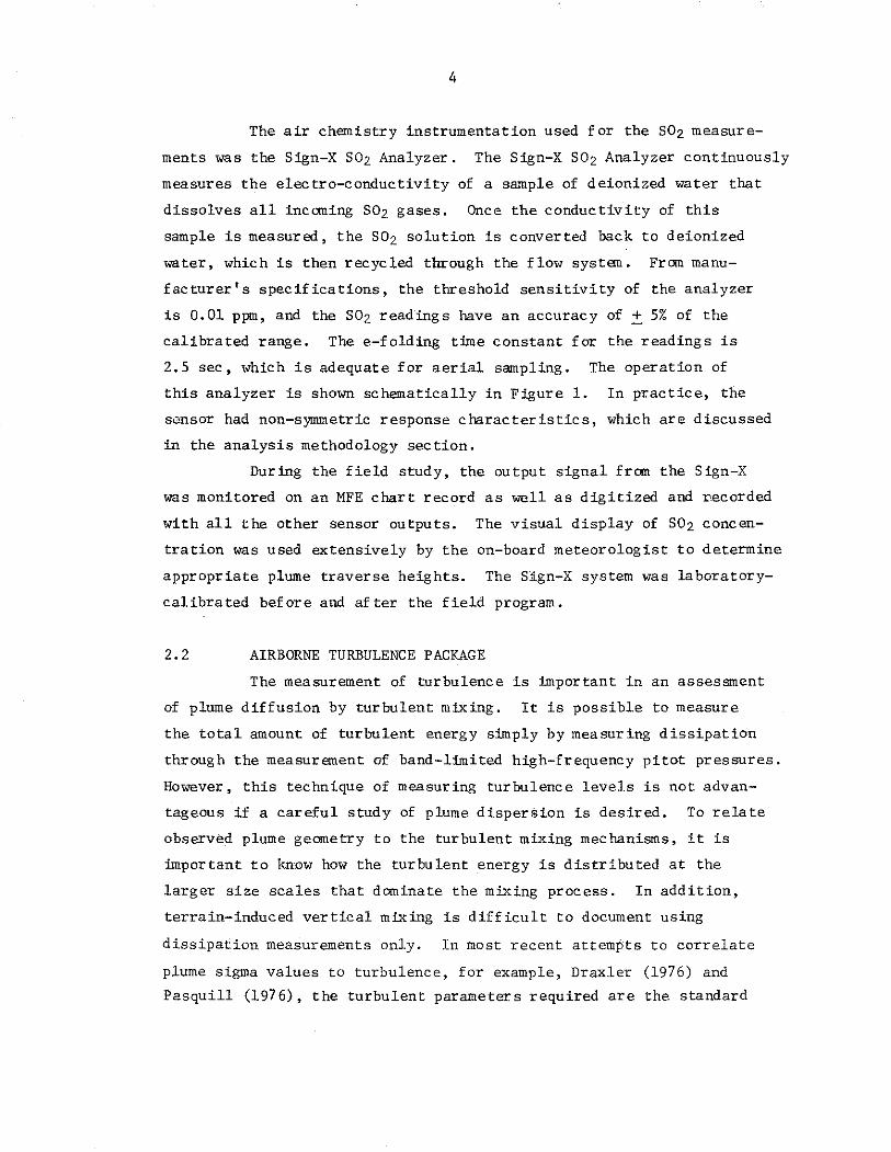


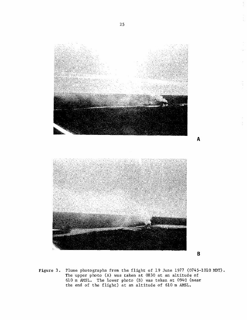


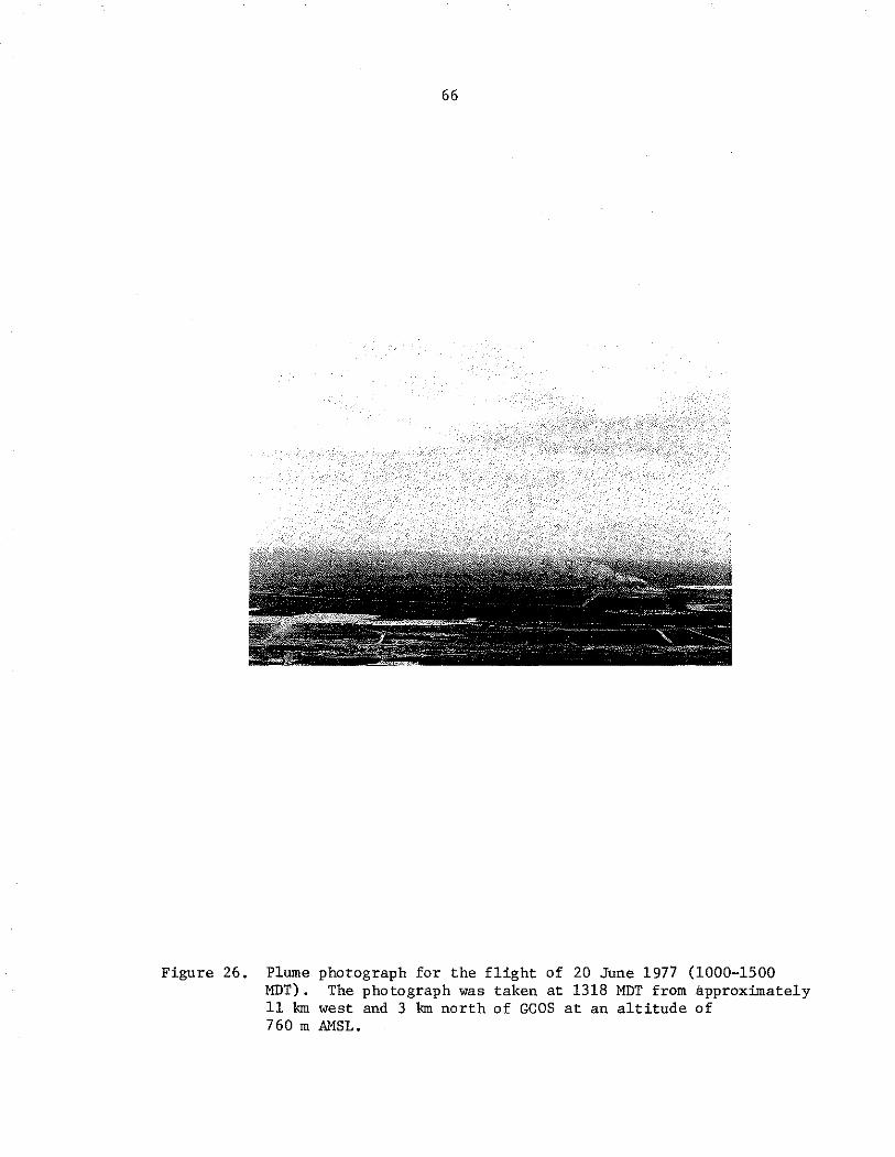


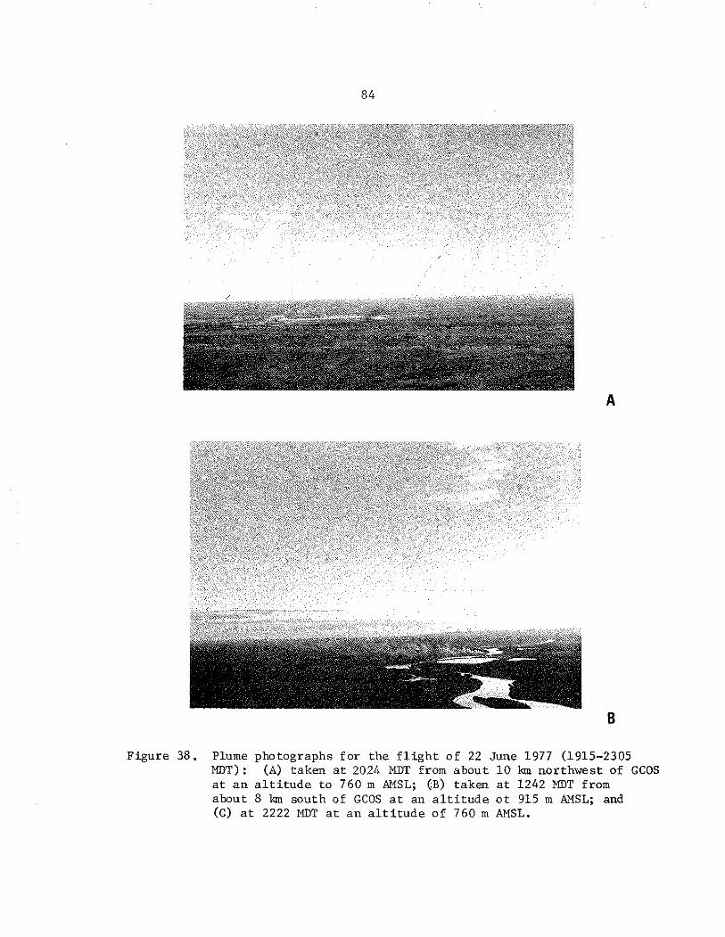

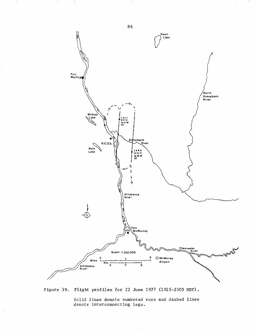


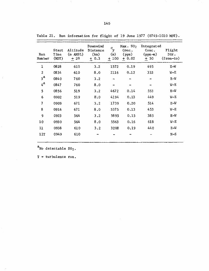


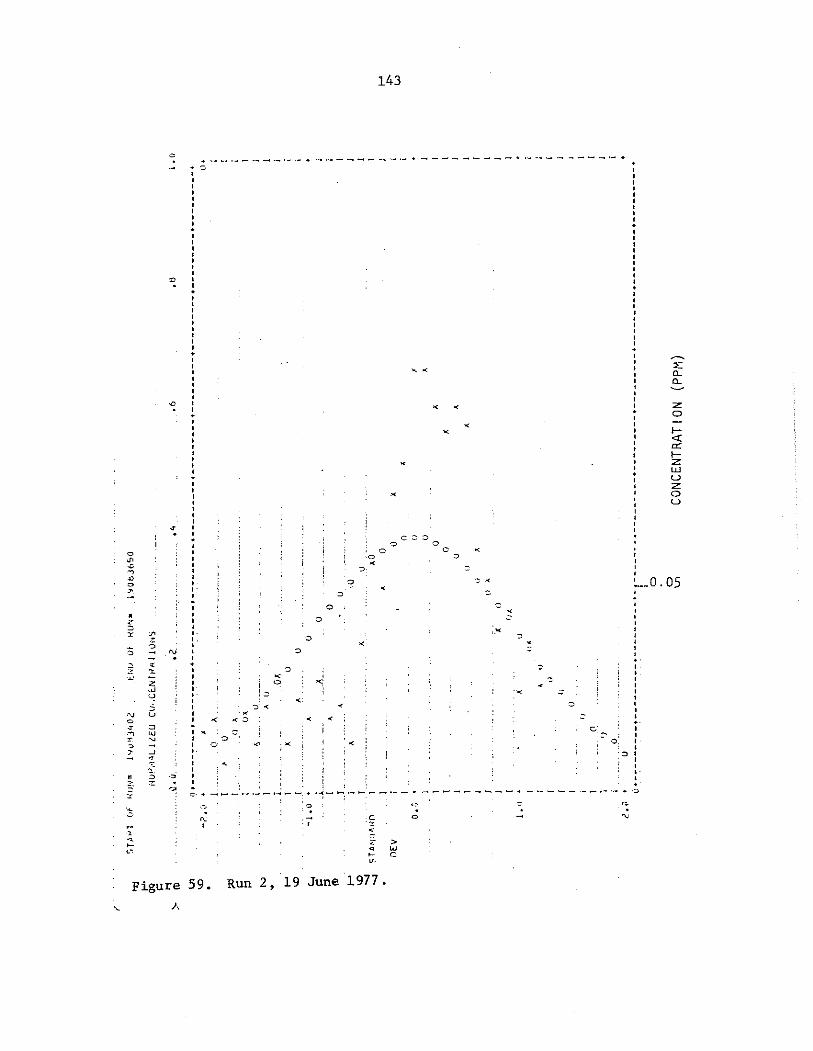


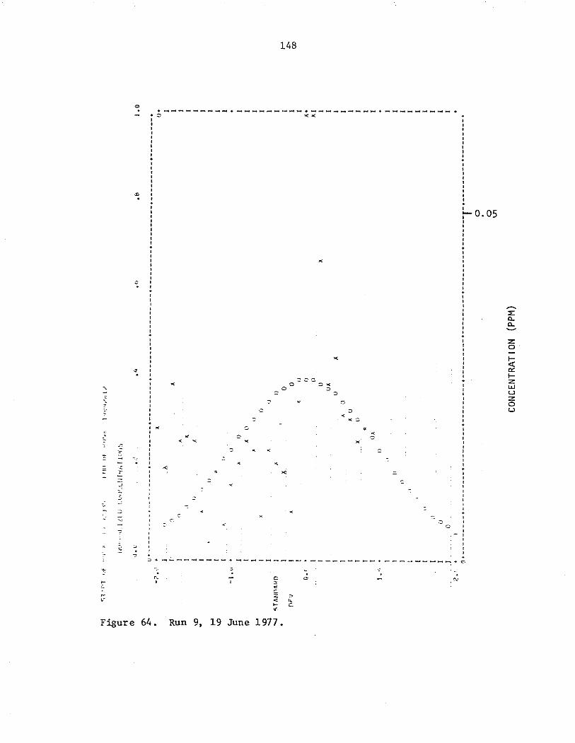


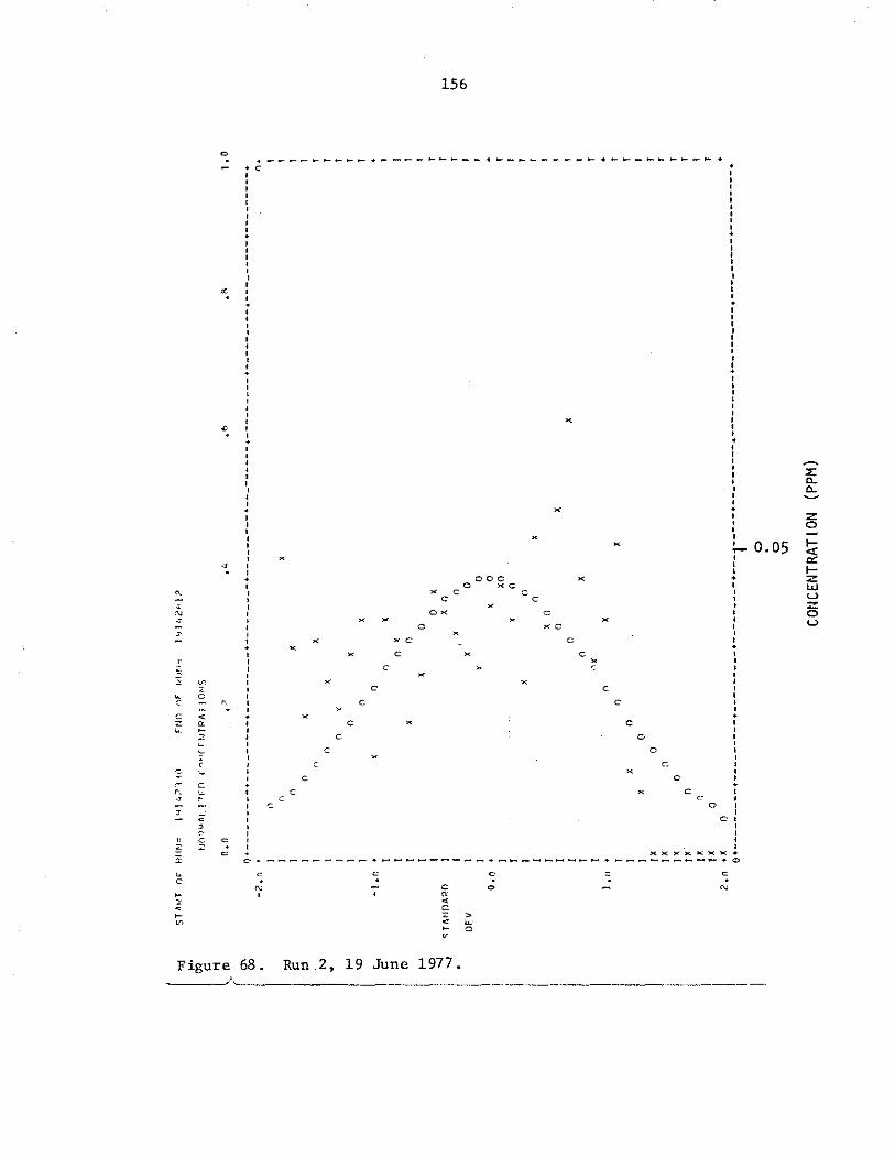


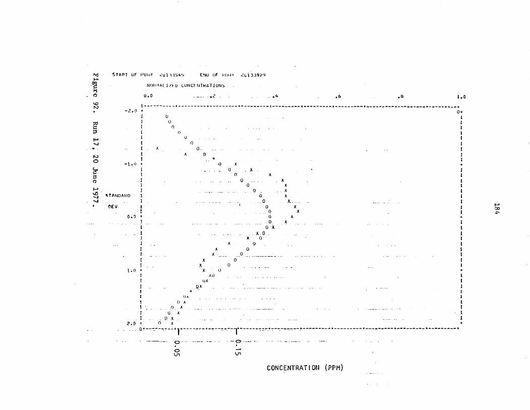


![Simultaneous dispersion measurements of multiple fiber ...dispersion measurement in a higher-order-mode fiber,” Opt. Lett. 37(3), 347–349 (2012). ... the fundamental [16] as it](https://img.dokumen.tips/doc/110x75/5f7f5ac01f1e4a75d5301076/simultaneous-dispersion-measurements-of-multiple-fiber-dispersion-measurement.jpg)


![Evaluating the impacts of SO emissions from power stations ... · measurements. Kho et al. [15] used the ISC-AERMOD dispersion model to predict air dispersion plumes from a diesel](https://img.dokumen.tips/doc/110x75/6094cd9c30fcea0f817f3a3d/evaluating-the-impacts-of-so-emissions-from-power-stations-measurements-kho.jpg)


![L 31 Light and Optics [1] Measurements of the speed of light The bending of light – refraction Dispersion Total internal reflection Dispersion Rainbows](https://img.dokumen.tips/doc/110x75/56649cbb5503460f949831cc/l-31-light-and-optics-1-measurements-of-the-speed-of-light-the-bending-of.jpg)

![L 33 Light and Optics [3] Measurements of the speed of light The bending of light – refraction Total internal reflection Dispersion Dispersion](https://img.dokumen.tips/doc/110x75/56649da85503460f94a94bf0/l-33-light-and-optics-3-measurements-of-the-speed-of-light-the-bending.jpg)


![L 34 Light and Optics [4] Measurements of the speed of light The bending of light – refraction Total internal reflection Dispersion Dispersion](https://img.dokumen.tips/doc/110x75/56649db25503460f94aa14db/l-34-light-and-optics-4-measurements-of-the-speed-of-light-the-bending.jpg)