Players-Econometricians, Adverse Selection, and

Equilibrium.

Jernej Copic ∗

February 14, 2014

Abstract

We study strategic environments of adverse selection, where in an outcome

of strategic interaction players-econometricians observe the distribution over

own payoffs and all players’ actions, and then form assessments regarding the

underlying uncertainty. Tailored to such situations where players may face

recovery problems, we define adverse equilibrium outcomes: players optimize,

their assessments are consistent, and they can justify one-another’s behavior.

We then study the problem from the perspective of an impartial econome-

trician who can only observe the distribution over the actions taken by the

players, and not their types. We define four conditions on the payoff structure

and the strategy profile: positivity, incentive imbalance, pooling, and infor-

mational adversity. These conditions characterize the environments where the

econometrician would reject equilibrium hypothesis if she didn’t take into ac-

count the recovery problem faced by the players.

∗jcopic@econ.ucla.edu. I am grateful to Andy Atkeson, Eddie Dekel, Faruk Gul, Jin Hahn, RosaMatzkin, Romans Pancs, and Bill Zame for helpful discussions, and to my students for encourage-ment. I am also grateful to the UCLA econometrics, macro, and theory-proseminar audiences.

1

JEL codes: C10, C70, D80

Keywords: consistency, recovery, adverse selection, equilibrium, incentives,

information.

1 Introduction

Ever since the publications of Akerlof’s (1970) “Market for Lemons”, Spence’s (1970)

“Job market signaling”, and Rothschild and Stiglitz’s (1976) “Equilibrium in Com-

petitive Insurance Markets”, various literatures have emerged documenting adverse

selection arising from asymmetric information as one of the fundamental problems of

information economics. In a nutshell, adverse selection describes the informational

problem resulting from an equilibrium whereby given the behavior of informed agents

on one side of the market, the uninformed agents on the other side cannot fully de-

duce private characteristics, or types, of the informed agents solely from observations

of what the informed agents do. These problems can be so severe to lead to market

breakdowns, or in the case of Rothschild and Stiglitz (1976), to non-existence of

equilibrium.1

One assumption underlying most of the literature on adverse selection and sig-

naling has been that the agents are nevertheless for some reason able to “know” the

true distribution of characteristics of the informed side of the market. To “know”

is meant in the sense of having a well-formed and accurate prior belief consistent

with the data. The problem is, however, that it is precisely the adverse selection

which might lead uninformed agents to face recovery problems2 regarding the under-

lying objective distribution of characteristics of the other side of the market. This,

in turn, would allow for the uninformed agents to have assessments different from,

1In a general-equilibrium setting, Zame (2007) shows that equilibrium in general exists.2We use the term “recovery”, in the sense of Mass-Colell, Whinston and Green (1995), to not

confuse with the econometric term “identification.” The latter is more general in that it may concernalso the payoff structure and the decision-making model itself, and not just the underlying uncertainparameters as is the case here.

2

yet entirely consistent with the truth (the objective joint distribution over agents’

characteristics), even when one assumes that the dataset at the uninformed agents’

disposal is comprised of infinitely many stationary observations with no additional

noise. In other words, in environments with asymmetric information, the assumption

that in an adverse-selection problem the agents’ assessments equal the truth may be

inconsistent with the informational problem of adverse selection itself.

The purpose of this paper is to address such strategic environments of adverse

selection, and study the problem from the perspective of an impartial econometrician

who can only observe the actions taken by the players, and not the realizations of

their types. The econometrician is thus much like the players themselves, and can

be imagined as one of the players in the game – such a player has no actual effect on

the outcome and a constant payoff function. What is meant by the econometrician’s

observation is an infinite dataset of observations of realizations of players’ actions.

The econometrician can therefore recover the distribution over players’ actions, what

we call the behavioral outcome. The question then is whether this distribution over

players’ actions could have been generated by equilibrium play of players facing the

recovery problem pertinent to adverse selection. That is, to test the equilibrium

hypothesis, under what conditions will the econometrician have to take into account

the recovery problem that such rational players – consistent econometricians face.

The focus of this paper is purely positive.

We provide a tight set of conditions characterizing environments with such re-

covery problems. These conditions pertain only to the underlying payoff structure

and the actual strategy profile that is played. Our main results then derive the

equilibrium outcomes and the corresponding behavior that an econometrician could

observe if these conditions are satisfied. The appropriate definition of adverse equilib-

rium outcomes is more complicated, as it involves an infinite regress of how players

justify all the privately observed parameters as arising from play of such rational

3

players – consistent econometricians.3 The definition of equilibrium is that players’

optimization and consistency of their assessments are common belief. This defini-

tion of adverse equilibrium is precisely tailored to the problem under consideration.

It is devoid of any exogenous assumptions regarding how players make assessments

from the infinite datasets that they are imagined to have accummulated. It is also

rigorously absent of any notion of irrationality or myopia.

Not surprisingly, if the players’ assessments were to coincide, then such equilib-

rium outcomes would be supportable in Bayes Nash equilibrium – the common prior

over uncertainty and strategies could then be imagined as such common assessments.

Of course, in that case, our econometrician would not need the present theory to test

the equilibrium hypothesis. We are therefore primarily interested in situations where

players’ assessments cannot coincide in an adverse equilibrium. Our conditions thus

provide a tight characterization of outcomes where Bayes Nash equilibrium would be

rejected, while adverse equilibrium would in fact be true.

The conditions that we provide here are of incentive- and informational nature.

On the incentive side, we provide two new notions, positivity and incentive imbalance.

A strategy profile is positive if for each player’s type, there is a draw of the other

players’ types such that the player’s strategy is in that state a best reply to the other

players’ strategies. Positivity is therefore an ex-post-type condition on the payoff

structure and the strategy profile. Incentive imbalance is a very simple and intuitive

condition guaranteeing that there is no common assessment of uncertainty, under

which a given strategy profile could simultaneously satisfy the incentive constraints

for all players. These two conditions provide a tight characterization of outcomes

that are not supportable in Bayes Nash equilibria, yet leave open the possibility of

adverse equilibrium with differing players’ assessments. The informational conditions

3Here we use the word “justify” rather than “rationalize” to not confuse such justification withthe standard notion of rationalizability, e.g., Bernheim (1984). As defined here, in such a justifica-tion a player considers not only the others’ possible behaviors but also their probabilistic consistencywith the outcomes of such behaviors.

4

are also pertinent to the payoff structure and the strategy profile, and are called

pooling and informational adversity. These guarantee that in such outcomes players

cannot recover the underlying uncertainty, so that their assessments can be different.

If an outcome satisfies these four conditions then it is not supportable in Bayes Nash

equilibrium, and it is supportable in adverse equilibrium. In two-player games this

characterization is tight.

This paper was inspired by studies in econometric theory, e.g., Manski (1993,

2004). These studies raise a concern as to how an impartial econometrician should

evaluate decision makers’ choices when decision makers face identification problems

(or recovery problems). The difference is that here we study equilibrium problems,

which is quite different, and we do not impose any exogenous identifying assumptions.

Instead, we treat the players’ estimation procedures by which they make their assess-

ments as a black box.4 The only requirement is that such an estimation procedure

satisfies asymptotic consistency, so that each agent can potentially hold a variety of

consistent assessments. Players are here standard expected-utility maximizers, who

play optimally under some such consistent assessment.

The definition of equilibrium here can be viewed as a version of minimal equilib-

rium given in Copic (2014) tailored to players in environments with adverse selection.

Adverse equilibrium can thus be viewed as a stationary steady state of any learning

process with no memory loss, where players make asymptotically consistent estimates

of the data they observe, players optimize, and justify the observed data as arising

from such other players. This definition of equilibrium could then also be viewed as

a refinement of the Self-confirming equilibrium in games with uncertainty, see Dekel

et al (2004). There, players are myopic in the sense that they do not justify their

observations as having arised from play by rational and consistent players. Adverse

equilibrium thus imposes additional constraints. In Section 6 we provide an exam-

4The present paper was also inspired by Anderson and Sonnenschein (1985), who consider ra-tional expectations equilibria of agents using linear econometric models.

5

ple demonstrating that adverse equilibrium outcomes are different from outcomes

that would require justification to any finite order rather than in an infinite regress

(in particular, demonstrating the difference with self-confirming equilibrium, which

requires no justification at all).5 That example also shows that our characteriza-

tion is tight: in such non-adverse-equilibrium outcomes our conditions are no longer

satisfied.

In Section 2 we describe the basic model and the econometric problem. In Sec-

tion ?? we give the definition of adverse equilibrium outcomes and some relationships

to Bayes Nash equilibrium outcomes. In Section 4 we give the incentive and infor-

mational conditions and our main results, theorems 1 and 2. In Section 5 we give

an example illustrating these results and an additional example illustrating how to

incorporate states of fundamentals of the economy in the model. In Section 5 we

discuss some generalizations of our conditions and results, and give the finite-order

example, which shows tightness of the statements of our theorems. Most of the

proofs are in the appendix.

2 The model and the econometric problem

In a game, we define the equilibrium concept, which is suited for studying situations

of adverse selection, i.e., where all players and an econometrician observe the players’

actions in an environment with uncertainty. Since a player’s strategy is a contingent

plan of action, given her private information, each player’s strategy is not directly

observable. What is observed by each player is the joint distribution over the player’s

own payoffs and actions of all players, conditional on the player’s own types. What

5Adverse equilibrium is also related to Self-confirming equilibrium, Fudenberg and Levine (1993),and especially Rationalizable Partition-Confirmed Equilibrium of Fudenberg and Kamada (2013),which is defined in extensive-form games with no uncertainty, allows for correlation in players’strategies, and takes into account players’ trembles. Less related are various notions of conjecturalequilibria, see e.g., Battigalli and Guatoli (1997), and Esponda (2013), and the notions in Jacksonand Kalai (1997) and Jehiel and Koessler (2008).

6

is observed by the econometrician is the behavioral outcome, which is the distribu-

tion over all players’ actions resulting from the underlying uncertainty and players’

contingent strategies. In this section, we begin by defining such environment, and

two benchmark cases, which are closely related to the standard model of Bayes Nash

equilibrium with a common prior.

A game, or the payoff structure, is Γ = {N,A,Θ, u}, where N = {1, ..., n} is

a finite set of players, A = ×i∈NAi is a product of finite sets of players’ actions,

Θ = ×i∈NΘi is the finite set of states of the world, i.e., a product of finite sets of

players’ payoff types, and u : A×Θ→ R|N | is a vector of players’ payoff functions.

The player indexed by n can be interpreted as the state of fundamentals of the

economy, in which case An ≡ {an}, un ≡ const., and in the payoff structure the types

of the other players are interpreted as their signals.6 S is the set of players’ mixed

strategies. Given an s ∈ S, s[θ] ∈ ∆(A) is the probability distribution over players’

actions when the draw of types is θ, and s[θ](a) is the probability of action profile

a, that is, s[θ](a) = ×i∈Nsi[θi](ai). To emphasize that any player can be thought of

also as an econometrician (or statistician), think of the disinterested econometrician

(a passive observer, who records the data) as player n + 1, in which case |Θn+1| =

|An+1| = 1, and un+1 ≡ const, where const is any constant. Γ is assumed to be

6The argument of how this is done is from Copic (2014), and we include it here for the sake ofcompleteness. Interpreting the state of the fundamentals of the economy as a player allows workingwithin the simpler normal-form representation with types alone, while preserving the generalityof the model that includes the states of fundamentals apart from players’ types or signals. The“types” of players 1, ..., n − 1 are then players’ signals, i.e., θi is the signal to player i when thestate of the world is θn, with the appropriate conditional payoff consequences to player i. Underthe usual Bayesian assumption of a common prior over the states of the world and the signalstructure, such signaling model is reducible to the normal-form payoff-type representation in thestandard way: by computing for each player the conditional expected payoffs for each vector ofsignals to all players. When there is no prior (and no common prior), as is the case here, suchstandard procedure is no longer possible, and different assessments may induce different normal-form representations. When the states of fundamentals are included as a “player,” that allows forsuch normal-form representation in the present case as well. This description therefore embeds thepresumably more general model with the states of fundamentals into a reduced-form frameworkwithout having to consider the states of fundamentals in any special way. In such representation,the states of fundamentals are indexed as “player n” rather than 0 because index 0 is here used todescribe the objective outcome. See also our second example in Section 5.

7

common knowledge.

An outcome of Γ is given by (P, s), P ∈ ∆(Θ), s ∈ S, and an outcome realization

is a draw (θ, a) ∼ (P, s); A behavioral outcome is given by a probability distribution

β ∈ ∆(A). Denote by PrP,s ∈ ∆(Θ×A) the probability distribution over types and

actions in an outcome (P, s), so that,

PrP,s(θ, a) = P (θ) s[θ](a), a ∈ A.

Given an outcome (P, s) ∈ ∆(Θ)×S, the behavioral outcome corresponding to (P, s)

is then given by βP,s ≡ PrP,sA , that is,7

βP,s(a) =∑θ∈Θ

P (θ)s[θ](a), a ∈ A.

For each player i, denote by Vi the set of i’s possible payoffs, i.e., Vi ≡ Image(ui),

and let V = ×i∈NVi.

In a game Γ, fix an outcome (P, s) ∈ ∆(Θ) × S, and imagine infinitely many

independent realizations of the outcome (P, s). Let ψ(.) be some statistic of the

outcome (P, s), where ψ maps onto some parameter space Ψ, so that ψ : Θ×A→ Ψ.

An ideal dataset is comprised of infinitely many independent observations of statistic

ψ.

Let P rP,s;T

ψ be the empirical distribution of T independent observations of the

statistic ψ, i.e., T independent realizations ψ(θt, at), t ∈ {1, ..., T}, where (θt, at) ∼

(P, s). Let P rP,s

ψ be the empirical distribution of ψ in the limit, as the number of

observations tends to ∞,

P rP,s

ψ = limT→∞

P rP,s;T

ψ .

7Throughout, the marginal distribution of some probability distribution Pr over a set X isdenoted by PrX , and the conditional is denoted by Pr|X .

8

By the Kolmogorov’s strong law of large numbers,

P rP,s

ψ ≡ PrP,sψ .

Here the statistic ψ will be of the form of a projection onto the parameter space

Ψ. It will then be convenient to use Ψ in the notation. In particular, if ψ(θ, a) =

(θi, a, ui(θ, a)), then Ψ = Θi×A× Vi, and PrP,sψ is then in a slight abuse of notation

simply the marginal probability distribution PrP,sΘi×A×Vi – note that PrP,s is a prob-

ability distribution over Θ × A, which naturally induces a probability distribution

over Θ× A× V .

As mentioned above, we imagine an econometrician simply as player n+ 1. The

econometrician assembles an ideal dataset of observations of statistic ψn+1 of the

outcome (P, s), and then adjudicates whether these observations could have been

generated by equilibrium play. Similarly, all players assemble ideal datasets of ob-

servations ψi, i ∈ N , and form consistent assessments. From such an assessment a

player can then deliberate the optimality of play of herself as well as others.

In the rest of this section we consider two benchmark cases. The first case is one

where ψBNi (θ, a) = (θ, a), so that ΨBNn ≡ Θ×A, ∀i ∈ N∪{n+1}. That is, all players

and the econometrician assemble ideal datasets of complete observations of realiza-

tions of the outcome. In this first benchmark case, as the number of observations

T → ∞, if each player uses any estimation procedure, which satisfies asymptotic

consistency, then it must be that their assessments equal the objective outcome. In

other words, there is no recovery problem as the observations of the realizations of

the outcome are complete.

In equilibrium, players must then optimize relative to the true objective outcome.

Moreover, each player can a fortiori justify the other players’ behavior: a player i

can attribute to player j the assessment over uncertainty given by (P, s), whereby

player j optimizes, and i can further ascertain that j could similarly attribute to any

9

other player k the assessment (P, s), whereby k optimizes, and so on. That is, there

is a common belief that players optimize and their assessments are fully consistent

with (P, s). Since each player’s assessment is (P, s), and each player optimizes, an

equilibrium outcome therefore coincides with a Bayes Nash equilibrium outcome.

In the second benchmark case, ψi(θ, a) = (θ, a), for all i ∈ N , but ψn+1(θ, a) = a,

or equivalently, ψn+1(θ, a) = (θn+1, a, un+1(θ, a)) (recall that a disinterested econo-

metrician only has one type and plays one action). By the same argument as before,

the behavior of players is still supportable in Bayes Nash equilibrium, but the econo-

metrician can no longer necessarily recover the true objective outcome. We can thus

reinterpret Bayes Nash equilibrium to encompass the two benchmark cases.

Given a (P, s) ∈ ∆(Θ)×S, denote by UP,si (θi, ai) the expected utility of player i,

when she is of type θi and plays action ai,

UP,si (θi, ai) =

∑θ−i∈Θ−i,a−i∈A−i

ui(ai, a−i, θi, θ−i)P (θ)×j 6=i sj[θj](aj).

Definition 1. A (P, s) ∈ ∆(Θ)× S is a Bayes-Nash equilibrium outcome, if,

UP,si (θi, ai) ≥ UP,s

i (θi, a′i),

∀ai, a′i ∈ Ai, s.t., si[θ](ai) > 0,∀θi ∈ Θi, s.t., P (θi) > 0, ∀i ∈ N.

A strategy profile s is supportable in Bayes-Nash equilibrium if there exists a P ∈

∆(Θ), such that (P, s) is a Bayes-Nash equilibrium outcome. A behavioral outcome

β ∈ ∆(A) is supportable in Bayes-Nash equilibrium, if there exists a (P, s) ∈ ∆(Θ)×

S, such that, (P, s) is a Bayes-Nash equilibrium outcome, and β = βP,s.

The subject of the next section is the case of interest, where each player also has

the ideal dataset of only partial observations of the outcome, and the econometrician

only observes the behavioral outcome. Then players, too, are facing a problem of

recovering the true outcome (P, s). A player has a greater scope of assessments that

10

are consistent with her observations and she may no longer be certain regarding

the strategy profile of the other players. Therefore, each player also has a greater

scope of assessments that justify each other’s behavior. We now make the formal

construction that corresponds precisely to this situation. From now on we consider

the problem from the perspective of the econometrician so that our focus will be on

what outcomes and consequent behavioral outcomes are supportable in equilibrium.

3 Adverse equilibrium

In the case of interest, apart from observing the other players’ behavior (the distri-

bution over their actions), each player also recovers the probability distribution over

her payoffs for each draw of her type, and for each action that she plays. Therefore,

ΨAEi = Θi×A×Vi, ∀i ∈ N . Since a player’s payoffs may vary with the other players’

types, a player can thus gain some additional information. Instead of focusing on

the statistic ΨAEi , we from now on focus simply on players’ information. Formally,

a player’s information is represented by the σ-algebra of events that she can discern

given the actual strategy profile played – a player can only obtain information from

the outcome realizations that have a positive probability.

Given an outcome (P, s) ∈ ∆(Θ)× s, denote by PrP,sΘi×A(θi, a) the probability of

θi ∈ Θi, a ∈ A, that is,

PrP,sΘi×A(θi, a) = PΘi(θi) si[θi](ai)×j 6=i

∑θj∈Θj

sj[θj](aj)

.

For θi ∈ Θi, a ∈ A, such that, PrP,sΘi×A(θi, a) > 0, let

V P,sθi,a

= {uθi,a(θ−i) | θ−i ∈ Θ−i, PΘi(θi) si[θi](ai)×j 6=i sj[θj](aj) > 0}.

Then, the information of i, conditional on her type θi and action profile a ∈ A, is

11

given by FP,sθi,a, the σ-algebra over Θ× A generated by the events,

{u−1θi,a

(v)× {(θi, a)} | v ∈ V P,sθi,a} ∪ ((Θi × A) \ {(θi, a)})×Θ−i.

For θi ∈ Θi, a ∈ A, such that, PrP,sΘi×A(θi, a) = 0, define FP,sθi,a= {Θ × A, ∅}. The

information of player i in an outcome (P, s) is given by,

FP,si,A = ∧θi∈Θi,a∈AFP,sθi,a.

Definition 2. Given (P, s), (P ′, s′) ∈ ∆(Θ) × S, (P ′, s′) is i − A-consistent with

(P, s), if,

∑(θ,a)∈E

P ′(θ)×i∈N s′i[θi](ai) =∑

(θ,a)∈E

P (θ)×i∈N si[θi], ∀E ∈ FP,si,A .

An assessment (P ′, s′) that is i − A-consistent with (P, s) can be thought of as

an assessment that player i made from her ideal dataset using some asymptotically

consistent procedure. That is, (P ′, s′) is i − A-consistent with (P, s), if and only if,

PrP′,s′

ΨAEi

(E) = PrP,sΨAE

i(E), ∀E ∈ FP,si,A . However, we make no assumption regarding

precisely what procedure a player used – there is no more information that can be

discerned from the ideal dataset barring exogenous assumptions. Thus, there is a

scope of different assessments that are i− A-consistent with (P, s).

Definition 3. For a given θi ∈ Θi, (P, s) satisfies θi-IC, if PΘi(θi) > 0 implies that,

UP,si (θi, ai) ≥ UP,s

i (θi, a′i), ∀ai, a′i ∈ Ai, s.t., si[θ](ai) > 0.

A (P, s) ∈ ∆(Θ)×S is optimal for i, or satisfies i-IC, if (P, s) satisfies θi-IC, ∀θi ∈ Θi.

The description of equilibrium behavior is now slightly more involved. Since

players do not know the underlying distribution over uncertainty, nor other players’

12

strategies, they make assessments regarding the outcome. In order to justify the other

players’ behavior, each player also makes higher order assessments, which describe

assessments that a player imputes on the other players.8 A construct is an infinite

hierarchy of such assessments. A first-order assessment of player i is denoted by

(P (i), s(i)) ∈ ∆(Θ)× S.

For k ∈ N, let Nk be the set of all sequences of length k with elements from

N ; for k = 0, define N0 = ∅. Let Li be the set of all finite sequences of integers

from N , such that the first element is i, and no two adjacent elements are the

same. That is, Li = {` ∈ Nk; k ≥ 1, `1 = i, `m+1 6= `m, 1 ≤ m < k}. Also, let

L = {` ∈ Nk; k ≥ 1, `m+1 6= `m, 1 ≤ m < k}, so that L = ∪i∈NLi. For ` ∈ L, define

first(`) as the first element of `, last(`) as the last element of `.

Let (P 0, s0) ∈ ∆(Θ) × S be the objective outcome. Player i’s construct is a

hierarchy of i’s assessments,

Ci = (P `, s`)`∈Li ∈ [∆(Θ)× S]Li

.

A profile of constructs is given by C = (C1, C2, ...Cn). Given ` ∈ L, first(`) = i,

C(`) = (P (`), s(`)) is i’s `-th order assessment. For example, when ` = (i), C(i) is the

assessment of player i about the outcome (P 0, s0). We adopt the convention that

P ∅ = P 0 and s∅ = s0, so that when ` = ∅, C(`) is the outcome of the game.

An objective outcome (P, s) is an adverse equilibrium outcome if at (P, s) each

player can hold a consistent assessment such that she optimizes, and such that she

can also believe that other players hold consistent assessments under which they

optimize, and so on, ad infinitum. That is, (P, s) is an adverse equilibrium outcome

if it admits a common belief in consistency and optimality.

8Here we define all assessments in the infinite hierarchy only over payoff-relevant uncertainty.This is without loss of generality, see Copic (2014), Theorem 3. As in Copic (2014), the equilibriumhere can be thought of as a stationary steady state of any learning process with no memory loss ofsophisticated rational players.

13

Definition 4. An outcome (P 0, s0) is an adverse equilibrium outcome of Γ if there

exists a supporting profile of constructs C, s.t.,

1. (P `, s`) satisfy j-IC, for j = last(`), for every ` ∈ L,

2. (P (i), s(i)) is i− A-consistent with (P 0, s0), for every i ∈ N , and,

3. (P (`,j), s(`,j)) is j −A-consistent with (P `, s`), for every j ∈ N , for every ` ∈ L.

A strategy profile s0 is supportable in adverse equilibrium if there exists a P (0) ∈

∆(Θ), s.t., (P 0, s0) is an adverse equilibrium outcome.

A behavioral outcome β ∈ ∆(A) is supportable in adverse equilibrium, if there exists

an adverse equilibrium outcome (P 0, s0), s.t., β ≡ βP0,s0 .

We now briefly outline some relevant relationships between the outcomes that

are supportable in adverse equilibrium and the two benchmark cases of the previous

section.

Proposition 1. Let (P 0, s0) be an adverse equilibrium outcome. Then, s0 is sup-

portable in Bayes Nash equilibrium, if and only if, there exists a supporting profile

of constructs C for (P 0, s0), C = (P `, s`)`∈L, such that, (P (i), s(i)) = (P (j), s(j)),

∀i, j ∈ N .

Proof. Let (P 0, s0) be a Bayes Nash equilibrium outcome. Then let (P `, s`) =

(P 0, s0), ∀` ∈ L. This profile of constructs satisfies the requirements of Definition 4.

In particular, (P (i), s(i)) = (P (j), s(j)), ∀i, j ∈ N .

For the converse, let (P 0, s0) be an adverse equilibrium outcome, with (P (i), s(i)) =

(P (j), s(j)), ∀i, j ∈ N . Denote (P (i), s(i)) = (P , s). By the requirement 1 of Definition

4, the outcome (P , s) is a Bayes Nash equilibrium outcome. By the requirement 2,

PΘi≡ P 0

Θiand si ≡ s0

i ,∀i ∈ N . Hence, s ≡ s0, and the claim follows.

Next, we provide a sufficient condition for the first-order assessments from Def-

inition 4 to coincide with the objective outcome. One may call such equilibrium

14

outcomes fully revealing.9 Define a conditionally-generic payoff structure as one

where for each type of each player and for each profile of actions, the payoff to that

player takes a different value for every profile of types of the other players.

Definition 5. Let Vθi,a = {uθi,a(θ−i) | θ−i ∈ Θ−i}. A payoff structure Γ is condi-

tionally generic if uθi,a : Θ−i → Vθi,a, is one-to-one, ∀θi ∈ Θi, ∀a ∈ A, ∀i ∈ N .

Proposition 2. Let the payoff structure Γ be conditionally generic and let (P 0, s0)

be an adverse equilibrium outcome. Then:

1. Every assessment in the supporting constructs from Definition 4 coincides with

the objective outcome, (P `s`) ≡ (P 0, s0),∀` ∈ L.

2. (P 0, s0) is a Bayes Nash equilibrium outcome.

Proof. To prove 1, take an i ∈ N , θi ∈ Θi, and a ∈ A, such that,

PΘi(θi) si[θi](ai)×j 6=i

∑θj∈Θj

sj[θj](aj)

> 0.

Since uθi,a : Θ−i → Vθi,a, is one-to-one, it follows that for each v ∈ Vθi,a, u−1θi,a

(v) =

{θ−i}, for some θ−i ∈ Θ−i. Therefore, FP,sθi,ais generated by the events

{(θi, a)} ∪ ((Θi × A) \ {(θi, a)})×Θ−i,

so that FP,si,A is generated by singletons. Hence, P ∗,iΘ−i|θi = P ∗Θ−i|θi and s∗,i−i ≡ s∗−i.

2 follows from 1 and Proposition 1.

9That is in the tradition of the literature on the Rational Expectations equilibrium, see e.g.,Radner (1982). However, it should be pointed out that that literature assumes a common prior overthe fundamental parameters, or, in the present sense, that economic agents’ assessments coincide.

15

4 Information and Incentive conditions of adverse

equilibrium outcomes

In this section we parse the incentive and informational conditions that describe

equilibrium behavior. Due to the recovery problem, adverse equilibrium outcomes

satisfy weaker conditions than the Bayes Nash equilibrium outcomes. In this main

section of the paper, we address the question under precisely what conditions an

outcome is supportable in adverse equilibrium, while it is no longer supportable in

Bayes Nash equilibrium. Our answer is a characterization of informationally-adverse

environments, that is, environments where due to equilibrium behavior players are

unable to recover the underlying distribution of uncertainty.

Of course, some adverse equilibrium outcomes are still supportable in Bayes Nash

equilibrium– if the econometrician assumed a common prior, she could explain the

players’ behavior even if such assumption wasn’t necessarily true. Other such out-

comes are no longer supportable in Bayes Nash equilibrium but are nonetheless

supportable in adverse equilibrium. Our primary concern are the outcomes of this

latter sort. Those are precisely the outcomes where, if the econometrician assumed

Bayes Nash equilibrium, she would falsely reject the equilibrium hypothesis.

Our first step is to characterize conditions under which a strategy profile s is not

supportable in Bayes Nash equilibrium of Γ but which still leave open the possibility

that s be supportable in adverse equilibrium of Γ. For instance, given a strategy

profile of the other players, a strategy for player i which is not a best reply for any

type draw will evidently not be supportable in Bayes Nash equilibrium of Γ. But such

a strategy of player i will also not satisfy incentive constraints for i. We first provide

a sufficient condition, which guarantees that a strategy profile is not supportable

in Bayes Nash equilibrium of Γ, but which rules out strategies that are never best

replies.

16

Let,

Θs,i = {θi ∈ Θi | ui(θi, θ−i, s′i, s−i)− ui(θi, θ−i, si, s−i) ≤ 0,∀s′i ∈ Si},

and let

Θs,θi = Θs,i ∩ [{θi} ×Θ−i] .

Thus, Θs,i ⊂ Θ is the set of draws of types θ for which i would not have any incentive

to deviate from si to some other strategy s′i, given s−i; and Θs,θi is the section of Θs,i

when player i’s type is θi.

Definition 6. A strategy profile s is positive, if Θs,θi 6= ∅, ∀θi ∈ Θi,∀i ∈ N .

Thus, a positive strategy profile might allow for player i to best-reply to other

players’ strategies if P ∈ ∆(Θ) put sufficient mass on Θs,i.

Proposition 3. If a strategy profile s ∈ S is supportable in Bayes Nash equilibrium

then s is positive.

Proof. If s is not positive, then there is an i ∈ N and a θi ∈ Θi, s.t., ui(θi, θ−i, s′i, s−i)−

ui(θi, θ−i, si, s−i) ≥ 0, ∀s′i ∈ Si. Therefore, no matter the conditional distribution

PΘ−i|θi , when player i is of type θi she would have an incentive to deviate. Thus, s

is not supportable in a Bayes Nash equilibrium of Γ.

The reverse implication is not true: a strategy profile s may be positive and it

may nonetheless not be supportable in Bayes Nash equilibrium.

Proposition 4. If a strategy profile s is not supportable in Bayes Nash equilibrium

of Γ, then for every θ ∈ Θ, there exists an i ∈ N , s.t., ui(θ, s′i, s−i)−ui(θ, si, s−i) > 0.

Proof. If there is a θ ∈ Θ, s.t., ui(θ, s′i, s−i) − ui(θ, si, s−i) ≤ 0, ∀i ∈ N , then set

P (θ) = 1, and s is supportable in a Bayes Nash equilibrium of Γ.

17

Corollary 1. If a strategy profile s is positive and is not supportable in Bayes

Nash equilibrium of Γ, then ∩i∈NΘs,i = ∅.

A sufficient condition for a strategy profile to not be supportable in Bayes Nash

equilibrium must also take into account the magnitude of players’ incentives. To do

that in a tractable way, the sufficient condition we provide here also slightly strength-

ens the necessary condition given by Corollary 1 to empty pair-wise intersections. For

a two-player game, along with the strategy profile being positive, the next condition

is then necessary and sufficient.

Take a game Γ, and suppose s ∈ S is positive. For each θi ∈ Θi, define αθi,s

as the minimal weight that must be assigned to Θs,θi , such that θi-IC may still be

satisfied. Formally,

αθi,s ≡ min{PΘ−i|θi(Θs,θi) | (P, s) satisfies θi − IC}.

Definition 7. A strategy profile s ∈ S is incentive-imbalanced in Γ if, Θs,i ∩Θs,j =

∅,∀i, j ∈ N , and,∑

i∈N1|Θi|

(∑θi∈Θi

αθi,s)> 1.

Proposition 5. Let s be positive and incentive-imbalanced in Γ. Then s is not

supportable in Bayes Nash equilibrium of Γ.

Proof. Assume (s, P ) is a Bayes Nash equilibrium outcome of Γ.

If Θs,i∩Θs,j = ∅,∀i, j ∈ N , this implies that∑

i∈N1|Θi|

(∑θi∈Θi

P|θi(Θs,θi))≤ 1, since

(P, s), satisfies i-IC for all i ∈ N , which is a contradiction.

As an observation, positivity and incentive imbalance together have specific geo-

metric implications on Γ and s. First, in order for a strategy profile to satisfy both

of these properties, it must be that |Θi| > 1, ∀i ∈ N . Otherwise, it is impossible to

simultaneously satisfy Θs,i ∩ Θs,j = ∅, ∀i, j ∈ N , and Θs,θi 6= ∅, ∀θi ∈ Θi, ∀i ∈ N .

Thus, to satisfy both, positivity and incentive imbalance, asymmetric information

must be two sided. Second, for a similar reason, it must be that for some players,

18

Θs,i is not a connected subset of Θ. That is most easily seen when N = 2. Our main

example of Section 5 of course satisfies these geometric properties.

Our next step is to provide conditions, which guarantee that a given strategy

profile s can be supported in adverse equilibrium, while possibly satisfying incentive

imbalance. These conditions must be of informational nature – in conditionally-

generic environments, by Proposition 2 players must in equilibrium correctly recover

the true underlying uncertainty. Then, such an outcome would have to be support-

able in Bayes Nash equilibrium outcome, contradicting Proposition 5. The following

conditions therefore guarantee that in equilibrium players can hold different assess-

ments of uncertainty. We focus on strategy profiles satisfying strong informational

requirements. In Section 6 we indicate to what extent these requirements can be

relaxed.

Given a strategy profile s ∈ S, define for each i ∈ N ,

As,∪i = ∪θi∈Θisupport(si[θi]),

and let As,∪ = ×i∈NAs,∪i .

Definition 8. Take a game Γ and a player i ∈ N . A strategy profile s ∈ S is

pooling for i, if,

ui(θ, ai, a−i) = ui(θ, a′i, a−i),∀ai, a′i ∈ A

s,∪i , ∀a−i ∈ As,∪−i ,∀θ ∈ Θ. (1)

A strategy profile s is pooling if it is pooling for all i ∈ N .

A strategy profile s is pooling for i, if for any profile of actions a−i that other

players play under s, i is for any of her types indifferent between all the actions that

she takes under si. In particular, if one of these actions is optimal for a given θi ∈ Θi,

then all the actions in As,∪i are optimal for θi, and i could play any mixed strategy

over As,∪i , when she is of type θi.

19

Definition 9. Take a game Γ. A strategy profile s ∈ S is informationally adverse,

if,

ui(θi, θ−i, a) = ui(θi, θ′−i, a),∀a ∈ As,∪,∀θi ∈ Θi,∀θ−i, θ′−i ∈ Θ−i,∀i ∈ N. (2)

A strategy profile s is informationally adverse if no player can recover any infor-

mation regarding the conditional distribution over the other players’ types from the

variation in her own payoffs. That is the case when for each of her types and actions

that she takes, her payoffs do not vary with the other players’ types. We can now

provide our main results.

Theorem 1. Take a game Γ and let s ∈ S be positive, pooling, and informationally

adverse.

Then, (P, s) is an adverse equilibrium outcome of Γ, for any P ∈ ∆(Θ).

Combining Theorem 1 and Proposition 5 we obtain the next corollary.

Corollary 2. If in addition to the requirements in Theorem 1, s is incentive im-

balanced, then s is supportable in adverse equilibrium of Γ, and s is not supportable

in Bayes Nash equilibrium of Γ.

The next theorem describes behavioral outcomes that are supportable in adverse

equilibrium but not in Bayes Nash equilibrium.

Theorem 2. A behavioral outcome β∗ ∈ ∆(A) is supportable in adverse equilibrium,

and is not supportable in Bayes Nash equilibrium of Γ, if there exists an outcome

(P, s), s.t., s is pooling, informationally adverse, positive, incentive imbalanced, and

β∗ = βP,sA .

Finally, we have the following proposition.

20

Proposition 6. Suppose that s0 ∈ S is pooling, informationally adverse, and

(s0, P 0) is an adverse equilibrium outcome of Γ. Then, for every P ∈ ∆(Θ) and

s ∈ S, if,

PrP0,s0

A ≡ PrP,sA , (3)

then outcome (P, s) is supportable in adverse equilibrium of Γ. Moreover, for every

P ∈ ∆(Θ), there exists an s satisfying (3).

Proposition 6 is of independent interest. Suppose a certain probability distri-

bution over players’ actions can arise in equilibrium play; An econometrician only

observes the marginal distribution over players’ actions. By the last claim in Proposi-

tion 6, under pooling and informational adversity, econometrician would have no way

of pinning down the underlying objective distribution over Nature’s moves. Hence,

barring the possibility to somehow gather additional information about P 0, there is

little scope for normative prescriptions.

5 Examples

In this section we provide two examples. Our first example illustrates our main

results. The example here is perhaps somewhat more complicated than would be

minimally required. All of the complication is to show the full scope of the results

of Section 4.

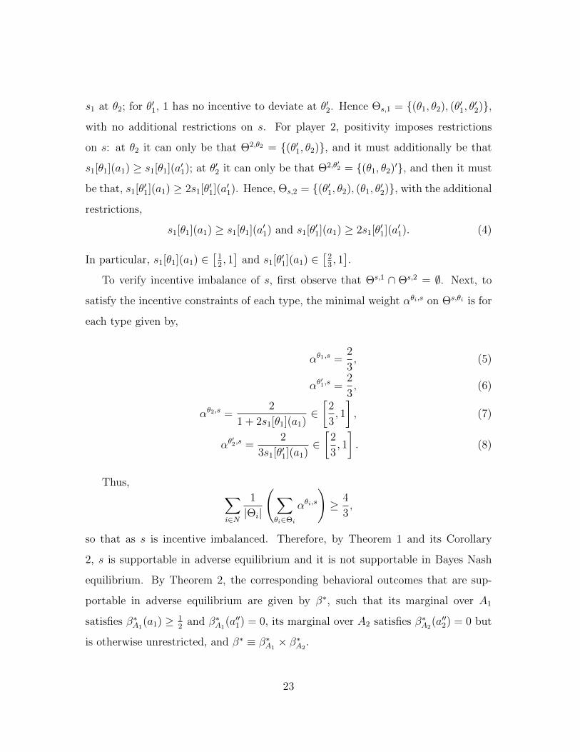
Each player i has 2 types, denoted by θi and θ′i, and 3 actions, denoted by ai, a′i,

and a′′i . We will focus on the outcomes where each player puts zero probability mass

on action a′′i , so that the payoffs associated with that action are relevant only in

terms of the deviations from other actions. All payoffs that are not important when

considering deviations from the other actions are chosen to be negative and constant,

equal to −1. The payoff structure is given by the four payoff matrices below.

21

(θ1, θ2) a2 a′2 a′′2

a1 1, 4 2, 4 −1, 6

a′1 1, 0 2, 0 −1, 2

a′′1 0,−1 1,−1 −1,−1

(θ1, θ′2) a2 a′2 a′′2

a1 1, 3 2, 3 −1, 2

a′1 1, 1 2, 1 −1, 2

a′′1 3,−1 4,−1 −1,−1

(θ′1, θ2) a2 a′2 a′′2

a1 2, 4 1, 4 −1, 3

a′1 2, 0 1, 0 −1, 2

a′′1 4,−1 3,−1 −1,−1

(θ′1, θ′2) a2 a′2 a′′2

a1 2, 3 1, 3 −1, 5

a′1 2, 1 1, 1 −1, 3

a′′1 1,−1 0,−1 −1,−1

Consider the strategy profile given by,

si = (si[.](ai), si[.](a′i)) ,

where si[.](ai) + si[.](a′i) = 1, i.e., each player i for each of her types mixes between

ai and a′i.

We first verify that this strategy profile satisfies pooling and informational ad-

versity. The actions that player i plays under s are As,∪i = {ai, a′i}. When player i is

either of type θi or θ′i, for each of her actions, her payoff does not vary with the other

players’ actions, so that s is pooling for both players, i.e., s is pooling. Next, for each

profile of actions a ∈ As,∪, each player’s payoff does not vary with the other players’

types, so that s satisfies informational adversity. Note also that each player i’s payoff

does not vary with her own actions (from As,∪i ), for each of her types, and for each

action played by the other player. Due to pooling and informational adversity, this

is of course a necessary condition for s to be an optimal strategy (but not necessarily

sufficient).

Next, we provide conditions on si[.] under which s is positive. For player 1, posi-

tivity imposes no restricitions on s: for θ1, player 1 has no incentives to deviate from

22

s1 at θ2; for θ′1, 1 has no incentive to deviate at θ′2. Hence Θs,1 = {(θ1, θ2), (θ′1, θ′2)},

with no additional restrictions on s. For player 2, positivity imposes restrictions

on s: at θ2 it can only be that Θ2,θ2 = {(θ′1, θ2)}, and it must additionally be that

s1[θ1](a1) ≥ s1[θ1](a′1); at θ′2 it can only be that Θ2,θ′2 = {(θ1, θ2)′}, and then it must

be that, s1[θ′1](a1) ≥ 2s1[θ′1](a′1). Hence, Θs,2 = {(θ′1, θ2), (θ1, θ′2)}, with the additional

restrictions,

s1[θ1](a1) ≥ s1[θ1](a′1) and s1[θ′1](a1) ≥ 2s1[θ′1](a′1). (4)

In particular, s1[θ1](a1) ∈[

12, 1]

and s1[θ′1](a1) ∈[

23, 1].

To verify incentive imbalance of s, first observe that Θs,1 ∩ Θs,2 = ∅. Next, to

satisfy the incentive constraints of each type, the minimal weight αθi,s on Θs,θi is for

each type given by,

αθ1,s =2

3, (5)

αθ′1,s =

2

3, (6)

αθ2,s =2

1 + 2s1[θ1](a1)∈[

2

3, 1

], (7)

αθ′2,s =

2

3s1[θ′1](a1)∈[

2

3, 1

]. (8)

Thus, ∑i∈N

1

|Θi|

(∑θi∈Θi

αθi,s

)≥ 4

3,

so that as s is incentive imbalanced. Therefore, by Theorem 1 and its Corollary

2, s is supportable in adverse equilibrium and it is not supportable in Bayes Nash

equilibrium. By Theorem 2, the corresponding behavioral outcomes that are sup-

portable in adverse equilibrium are given by β∗, such that its marginal over A1

satisfies β∗A1(a1) ≥ 1

2and β∗A1

(a′′1) = 0, its marginal over A2 satisfies β∗A2(a′′2) = 0 but

is otherwise unrestricted, and β∗ ≡ β∗A1× β∗A2

.

23

Our second example is very simple. It is intended to illustrate how to include the

states of the fundamentals of the economy in the game, even while that is in a way

evident.10 The example also shows the distinction between a Bayes Nash equilibrium

outcome and a strategy being supportable in Bayes Nash equilibrium. In this exam-

ple, there are 2 players, where “player 2” represents the states of the fundamentals

of the economy – player 2 has one “action,” called O, and player 1 has 2 actions, up

or down. Each player has 2 types. The types of player 2 represent the state of the

fundamentals of the economy, and the types of player 1 are the corresponding signals

to player 1. The states are given by the low state θ2 and the high state θ2, and the

corresponding signals to player 1 are θ1 and θ1. For the sake of the example, assume

that the signals are entirely uninformative of the state of the fundamentals, i.e., the

objective distribution P is uniform over Θ. The payoff structure is given by the four

matrices below (const. is any constant),

(θ1, θ2) O

up 0, const.

down 1, const.

(θ1, θ2) O

up 3, const.

down 1, const.

(θ1, θ2) O

up 0, const.

down 1, const.

(θ1, θ2) O

up 3, const.

down 1, const.

This example is therefore effectively a decision problem entertained by player

1. Depending on player 1’s strategy, i.e., the action that she plays for each of her

signals, she may or may not be able to recover the underlying objective distribution

over the uncertainty. In fact, if s∗ ≡ (up,O), then (s∗, P ) is a Bayes Nash equilibrium

10Still, it is important to keep in mind that if signals are purely informational, so that thereis no taste-shock component in the signal, then the player’s preferences depend only on the stateof the fundamentals. One could of course also explicitly include a taste-shock component in thesignal, however, that would be unnecessary as such case could always be represented by simplyadding additional states of the fundamentals with the appropriate conditional distribution over theplayers’ signals.

24

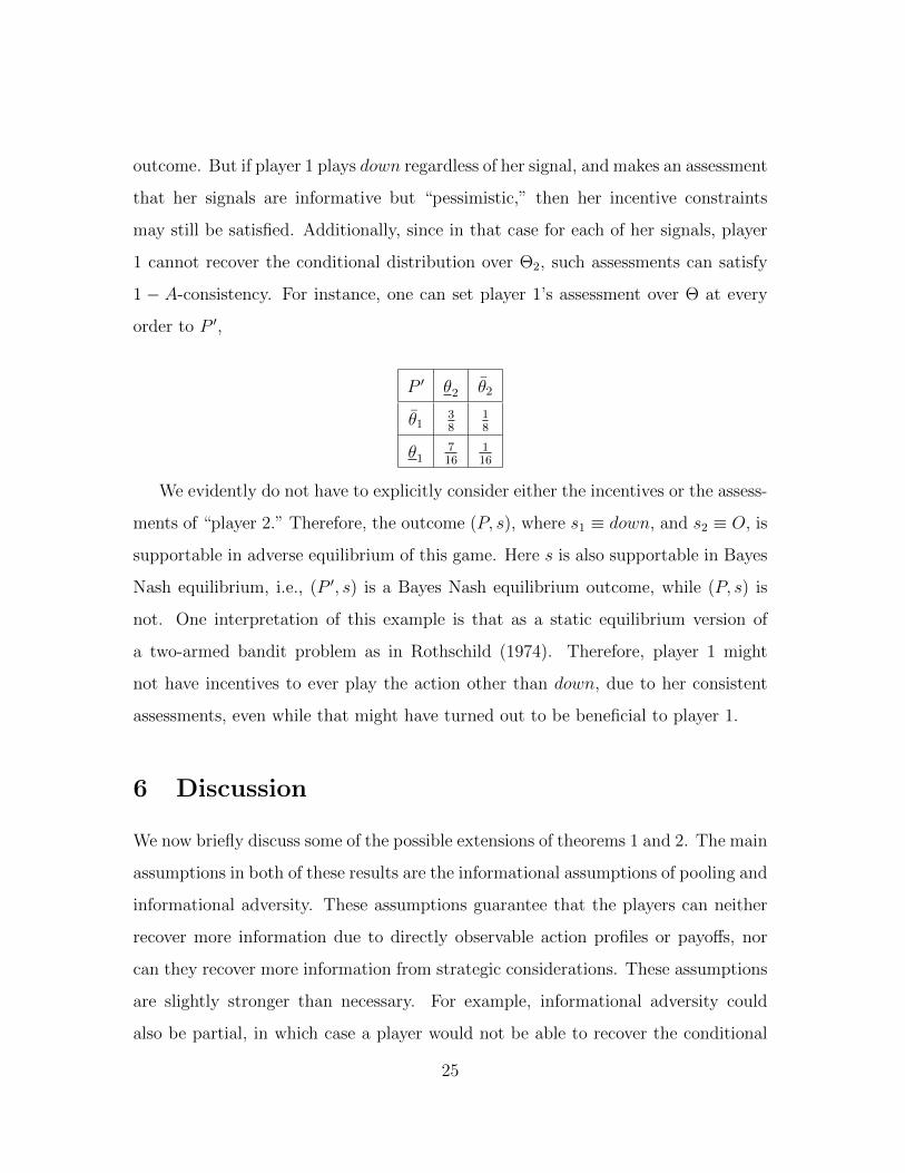
outcome. But if player 1 plays down regardless of her signal, and makes an assessment

that her signals are informative but “pessimistic,” then her incentive constraints

may still be satisfied. Additionally, since in that case for each of her signals, player

1 cannot recover the conditional distribution over Θ2, such assessments can satisfy

1 − A-consistency. For instance, one can set player 1’s assessment over Θ at every

order to P ′,

P ′ θ2 θ2

θ138

18

θ1716

116

We evidently do not have to explicitly consider either the incentives or the assess-

ments of “player 2.” Therefore, the outcome (P, s), where s1 ≡ down, and s2 ≡ O, is

supportable in adverse equilibrium of this game. Here s is also supportable in Bayes

Nash equilibrium, i.e., (P ′, s) is a Bayes Nash equilibrium outcome, while (P, s) is

not. One interpretation of this example is that as a static equilibrium version of

a two-armed bandit problem as in Rothschild (1974). Therefore, player 1 might

not have incentives to ever play the action other than down, due to her consistent

assessments, even while that might have turned out to be beneficial to player 1.

6 Discussion

We now briefly discuss some of the possible extensions of theorems 1 and 2. The main

assumptions in both of these results are the informational assumptions of pooling and

informational adversity. These assumptions guarantee that the players can neither

recover more information due to directly observable action profiles or payoffs, nor

can they recover more information from strategic considerations. These assumptions

are slightly stronger than necessary. For example, informational adversity could

also be partial, in which case a player would not be able to recover the conditional

25

distribution over the other players’ types only for some subset of the other players’

types. Similarly, pooling could be partial, to the extent that there existed at least one

action that were optimal for all types of a player. Then, each player might be able

to partly recover the conditional distribution over the other players’ types from the

behavior of these other players, but there would be some residual recovery problem

– e.g., in a two-player game, the player would be unable to determine which type of

the other player played the one action that all types could play, so that the player

would be unable to invert the observed probability of play of that action. We do not

formally describe these extensions here as that would require a substantial amount

of additional notation and definitions.11

One important point, which we here discuss in some more detail, is that the

informational conditions as given in theorems 1 and 2 must hold across all types (for

all actions that are played). The reason for that can be found in the proofs of these

results: in order for players to be able to justify one-another’s behavior in an infinite

regress, at each level of reasoning, the appropriate (minimal) amount of probability

mass must be assigned to the positive sets of player under consideration. Therefore,

the probability mass must be assigned and reassigned between these different positive

sets in a way that satisfies i−A-consistency. If informational adversity and pooling

do not hold accross all types and actions that are played, then it is no longer possible

to do so ad-infinitum. Thus, while the informational conditions depend only on the

payoff structure and the strategy profile, the reasons why these conditions are as

they are stem from the infinite regress of common belief. We illustrate this with the

following example.12

Consider the game given by the payoff structure below, and consider the strategy

11To write down results analogous to theorems 1 and 2, one would also have to specify conditionssuch that on the set of types where there is no recovery problem, the resulting behavior is sup-portable in Bayes Nash equilibrium. The combination of these conditions is not too difficult butrequires a large amount of additional notation, and the statements themselves are rather lengthy.

12This example is similar to an example in Copic (2012).

26

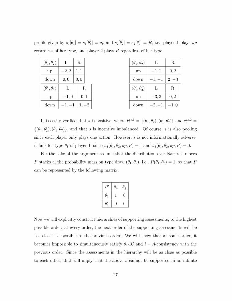
profile given by s1[θ1] = s1[θ′1] ≡ up and s2[θ2] = s2[θ′2] ≡ R, i.e., player 1 plays up

regardless of her type, and player 2 plays R regardless of her type.

(θ1, θ2) L R

up −2, 2 1, 1

down 0, 0 0, 0

(θ1, θ′2) L R

up −1, 1 0, 2

down −1,−1 2,−3

(θ′1, θ2) L R

up −1, 0 0, 1

down −1,−1 1,−2

(θ′1, θ′2) L R

up −3, 3 0, 2

down −2,−1 −1, 0

It is easily verified that s is positive, where Θs,1 = {(θ1, θ2), (θ′1, θ′2)} and Θs,2 =

{(θ1, θ′2), (θ′1, θ2)}, and that s is incentive imbalanced. Of course, s is also pooling

since each player only plays one action. However, s is not informationally adverse:

it fails for type θ1 of player 1, since u1(θ1, θ2, up,R) = 1 and u1(θ1, θ2, up,R) = 0.

For the sake of the argument assume that the distribution over Nature’s moves

P stacks al the probability mass on type draw (θ1, θ2), i.e., P (θ1, θ2) = 1, so that P

can be represented by the following matrix,

P ′ θ2 θ′2

θ1 1 0

θ′1 0 0

Now we will explicitly construct hierarchies of supporting assessments, to the highest

possible order: at every order, the next order of the supporting assessments will be

“as close” as possible to the previous order. We will show that at some order, it

becomes impossible to simultaneously satisfy θ1-IC and i − A-consistency with the

previous order. Since the assessments in the hierarchy will be as close as possible

to each other, that will imply that the above s cannot be supported in an infinite

27

hierarchy. Since s is such that each player only plays one action, in order for i− A-

consistency to hold, the strategy profile smust here effectively be common knowledge,

i.e., s` ≡ s, ∀` ∈ L. It is therefore enough to specify only the supporting assessments

over Θ.

First, (P, s) satisfies 1-IC but does not satisfy 2-IC, which fails for the type θ2.

We therefore set P (1) = P . To satisfy 2-IC along with 2− A-consistency, P (2) must

assign at least equal probabilities to type draws (θ1, θ2) and (θ′1, θ2), and by 2 − A-

consistency it must assign marginal probability 0 to type θ2. Hence, the following

P (2) is on the boundary of admissible first-order supporting assessments for Player

2,

P (2) θ2 θ′2

θ112

0

θ′112

0

By this same argument, it must be that P (12) = P (2), and by a similar argument,

applied to type θ′1 of player 1, the closest admissible supporting assessment P (21) to

P (2) is given by,

P (21) θ2 θ′2

θ112

0

θ′114

14

Similarly, at order 3, P (121) = P (21), and P (212) is given by,

P (212) θ2 θ′2

θ138

18

θ′138

18

At order 4, P (1212) = P (212), and P (2121) is given by,

28

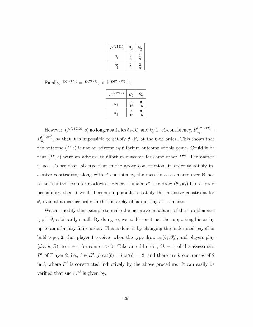
P (2121) θ2 θ′2

θ138

18

θ′128

28

Finally, P (12121) = P (2121), and P (21212) is,

P (21212) θ2 θ′2

θ1516

316

θ′1516

316

However, (P (21212), s) no longer satisfies θ1-IC, and by 1−A-consistency, P(121212)|θ1 ≡

P(21212)|θ1 , so that it is impossible to satisfy θ1-IC at the 6-th order. This shows that

the outcome (P, s) is not an adverse equilibrium outcome of this game. Could it be

that (P ′, s) were an adverse equilibrium outcome for some other P ′? The answer

is no. To see that, observe that in the above construction, in order to satisfy in-

centive constraints, along with A-consistency, the mass in assessments over Θ has

to be “shifted” counter-clockwise. Hence, if under P ′, the draw (θ1, θ2) had a lower

probability, then it would become impossible to satisfy the incentive constraint for

θ1 even at an earlier order in the hierarchy of supporting assessments.

We can modify this example to make the incentive imbalance of the “problematic

type” θ1 arbitrarily small. By doing so, we could construct the supporting hierarchy

up to an arbitrary finite order. This is done is by changing the underlined payoff in

bold type, 2, that player 1 receives when the type draw is (θ1, θ′2), and players play

(down,R), to 1 + ε, for some ε > 0. Take an odd order, 2k − 1, of the assessment

P ` of Player 2, i.e., ` ∈ L2, first(`) = last(`) = 2, and there are k occurences of 2

in `, where P ` is constructed inductively by the above procedure. It can easily be

verified that such P ` is given by,

29

P ` θ2 θ′2

θ12k−1+1

2k+12k−1−1

2k+1

θ′12k−1+1

2k+12k−1−1

2k+1

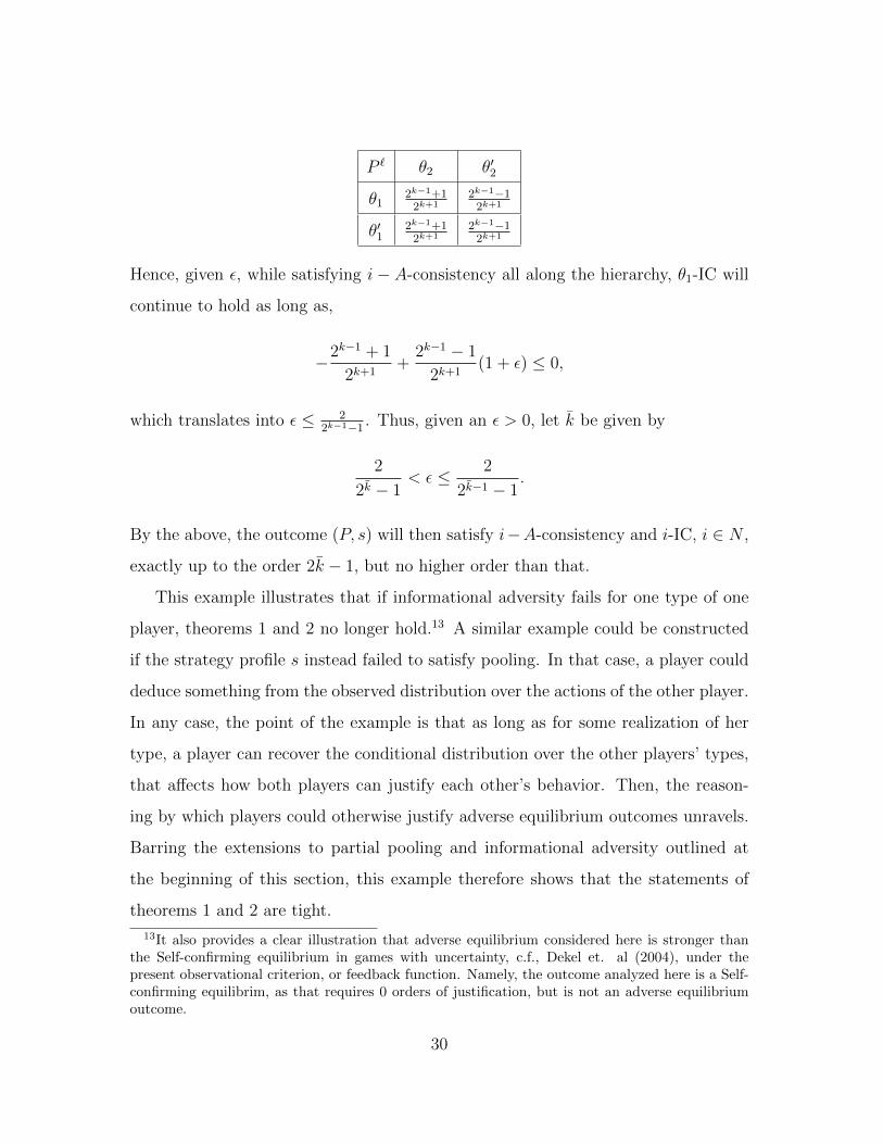
Hence, given ε, while satisfying i− A-consistency all along the hierarchy, θ1-IC will

continue to hold as long as,

−2k−1 + 1

2k+1+

2k−1 − 1

2k+1(1 + ε) ≤ 0,

which translates into ε ≤ 22k−1−1

. Thus, given an ε > 0, let k be given by

2

2k − 1< ε ≤ 2

2k−1 − 1.

By the above, the outcome (P, s) will then satisfy i−A-consistency and i-IC, i ∈ N ,

exactly up to the order 2k − 1, but no higher order than that.

This example illustrates that if informational adversity fails for one type of one

player, theorems 1 and 2 no longer hold.13 A similar example could be constructed

if the strategy profile s instead failed to satisfy pooling. In that case, a player could

deduce something from the observed distribution over the actions of the other player.

In any case, the point of the example is that as long as for some realization of her

type, a player can recover the conditional distribution over the other players’ types,

that affects how both players can justify each other’s behavior. Then, the reason-

ing by which players could otherwise justify adverse equilibrium outcomes unravels.

Barring the extensions to partial pooling and informational adversity outlined at

the beginning of this section, this example therefore shows that the statements of

theorems 1 and 2 are tight.

13It also provides a clear illustration that adverse equilibrium considered here is stronger thanthe Self-confirming equilibrium in games with uncertainty, c.f., Dekel et. al (2004), under thepresent observational criterion, or feedback function. Namely, the outcome analyzed here is a Self-confirming equilibrim, as that requires 0 orders of justification, but is not an adverse equilibriumoutcome.

30

7 Appendix

We first prove two preliminary lemmas and a proposition.

Lemma 1. Suppose s ∈ S is informationally adverse. Then, for s′ ∈ S, P, P ′ ∈ ∆(Θ),

and i ∈ N , the following are equivalent.

1. (P, s) is i− A-consistent for i with (P ′, s′).

2. PrP,sA ≡ PrP′,s′

A , P ′Θi≡ PΘi

and s′i ≡ si.

3. PrP,sAi|θi ≡ PrP′,s′

Ai|θi , P′Θi≡ PΘi

and s′i ≡ si.

Proof. That 1 implies 2 is obvious, 2 implies 3 because players’ strategies are uncor-

related, and 3 implies 1 by informational adversity.

Lemma 2. Take s ∈ S, P, P ′ ∈ ∆(Θ), i ∈ N , and suppose P ′Θi≡ PΘi

. Then there

exists an s′ ∈ S, such that, PrP′,s′

A−i|θi ≡ PrP,sA−i|θi and s′i ≡ si.

Proof. Let β = βP,sA . For each θi ∈ Θi set s′i[θi] ≡ si[θi], and set s′−i[θ−i] ≡ βA−i,

∀θ−i ∈ Θ−i.

Proposition 7. Let Γ be given, with |Θi| ≥ 2, ∀i ∈ N . Take a P 0 ∈ ∆(Θ) and a

strategy profile s0 ∈ S. Suppose s0 is pooling, informationally adverse, and for every

i ∈ N , there exists an assessment (P (i), s(i)), such that, (P (i), s(i)) satisfies i-IC, and,

(P (i), s(i)) is i− A-consistent with (P 0, s0).

Then (P 0, s0) is an adverse equilibrium outcome of Γ.

Proof. The proof is by induction. The base of induction is true by assumption. So

take a k ≥ 0, and suppose that for every order of assessments ` ∈ L, s.t., |`| ≤ k,

(P (`,i), s(`,i)) is i−A-consistent with (P (`), s(`)), and (P (`,i), s(`,i)) satisfies i-IC, ∀i ∈ N .

Take j 6= i. If there exists a k′ ≤ k, s.t., `k′ = j, then let `′ = `{1,...,k′}; otherwise let

31

`′ = (j). That is, k′ is the index of last previous occurrence in `, if such an occurrence

exists. Now let,

P(`,i,j)Θi|θj ≡ P

(`′)Θi|θj , P

(`,i,j)(θj) ≡ P (`,i)(θj),∀θj, s(`,i,j)j ≡ s

(`′)j ,

and by Lemma 1 and 2, we can set s(`,i,j)i so that (P (`,i,j), s(`,i,j)) is A− j-consistent

with (P (`,i), s(`,i)). Since k′ ≤ k, by inductive assumption, (P (`), s(`)) satisfies IC-j,

which implies that (P (`,i,j), s(`,i,j)) satisfies IC-j.

Proof of Theorem 1. Take a P 0 ∈ ∆(Θ). We will show that there exist assessments

(P (i), s(i)), i ∈ N , such that the requirements of Proposition 7 are satisfied.

Take i ∈ N , θi ∈ Θi, and let P(i)Θ−i|θi be any probability distribution over Θ−i,

s.t., P(i)Θ−i|θi(Θ

s,θi) = αθi,s0, and the incentive constraint for θi is satisfied. Since s0

is positive, such a P(i)Θ−i|θi exists for each θi ∈ Θi. Now set the marginal probability

P(i)Θi

(θi) = P 0Θi

(θi), ∀θi ∈ Θi, and this determines P (i). To define strategy assessments,

set s(i) by applying Lemma 2, and by Lemma 1, (P (i), s(i)) is i − A-consistent with

(P 0, s0), for all i ∈ N . Thus, requirements of Proposition 7 are satisfied.

What remains to be shown is that assessment (P (i), s(i)) satisfies i-IC, ∀i ∈ N .

Take a θi ∈ Θi. Since s0 satisfies pooling for i, and since (P (i), s(i)) is i−A-consistent

(P 0, s0),

∑θ−i∈Θ−i

ui(θi, θ−i; ai, s(i)−i)P

(i)Θ−i|θi(θ−i) =

∑θ−i∈Θ−i

ui(θi, θ−i; ai, s0−i)P

(i)Θ−i|θi(θ−i),

∀ai ∈ As0,∪i . By construction (P (i), s0) satisfies i-IC, and by Lemma 1, As

0,∪i ≡ As

(i),∪i ,

so that (P (i), s(i)) satisfies i-IC.

Proof of Proposition 6. Take P ∈ ∆(P ) and s ∈ S, s.t., PrP,sA ≡ PrP0,s0

A . Take

i ∈ N and θi ∈ Θi. Since (P 0, s0) is supportable in adverse equilibrium, there exists

a (P (i), s(i)), s.t., s(i) satisfies i-IC, and (P (i), s(i)) is i−A-consistent with (P 0, s0), so

32

that in particular, s0i ≡ s(i). Since s0 is informationally adverse,

ui(θi, θ−i, a) = ui(θi, θ−i, a),∀a ∈ As0,∪,∀θ−i, θ′−i ∈ Θ−i.

Hence, by Lemma 1 we obtain,

EPΘ−iEβ−i

ui(θi, θ−i, ai, a−i) = EP ′Θ−iEβ−i

ui(θi, θ−i, ai, a−i), (9)

∀ai ∈ ∆(As0,∪i ),∀β−i ∈ ∆(As

0,∪−i ),∀P ′Θ−i

, P ′′Θ−i∈ ∆(Θ−i). Let β0 = PrP

0,s0

A , define

si[θi] ≡ si[θi], ∀θi ∈ Θi, and define s(i)−i ≡ β∗A−i

. Next let P(i)Θ−i|θi ≡ P

(i)Θ−i|θi ,∀θi ∈ Θi,

and P(i)Θi

= PΘi. By (9), (P (i), s(i)) satisfies i-IC, because (P (i), s(i)) satisfies i-IC, and

(P (i), s(i)) is consistent for i with (P, s). The proof follows from Proposition 7.

Proof of Theorem 2. That β∗ is supportable in a-consistent Nash equilibrium of Γ

follows from Theorem 1 and Proposition 6. Take a (P, s), s.t., PrP,sA ≡ β∗. Since s0

satisfies pooling it follows that s satisfies pooling, which implies that Θs,i = Θs0,i,∀i ∈

N , and consequently s is also incentive imbalanced. Therefore, β∗ is not supportable

in Bayes Nash equilibrium of Γ.

References

[1] Akerlof, G. A. [1970]: “The Market for “Lemons”: Quality Uncertainty and

the Market Mechanism,” Quarterly Journal of Economics, 84, 488 - 500.

[2] Anderson, R. M. and H. Sonnenschein [1985]: “Rational Expectations

Equilibrium with Econometric Models,” Review of Economic Studies, 52, 359 -

369.

33

[3] Battigalli, P. and D. Guatoli [1997]: “Conjectural Equilibria and Ratio-

nalizability in a Game with Incomplete Information,” in Decisions, Games and

Markets, Kluwer Academic Publishers, Norwell, MA.

[4] Bernheim, D. B. [1984]: “Rationalizable Strategic Behavior,” Econometrica,

52, 1007-1028.

[5] Brandenburger, A. and E. Dekel [1993]: “Hierarchies of Beliefs and Com-

mon Knowledge, Journal of Economic Theory 59, 189-198.

[6] Copic, J. [2012]: “Nash equilibrium, rational expectations, and heterogeneous

beliefs: Action-consistent Nash equilibrium,” mimeo.

[7] Copic, J. [2013]: “Two-sided adverse selection,” mimeo.

[8] Copic, J. [2014]: ‘Normal-form Games with Decentralized Rational Statisti-

cians: Moral hazard and Adverse selection,” mimeo.

[9] Dekel E., D. Fudenberg, and D. K. Levine [2004]: “Learning to Play

Bayesian Games,” Games and Economic Behavior, 46, 282303.

[10] Esponda, I. [2013]: “Rationalizable Conjectural Equilibrium: A Framework

for Robust Predictions,” Theoretical Economics, forthcoming.

[11] Fudenberg D. and Y. Kamada [2013]: “Rationalizable Partition-Confirmed

Equilibrium,” mimeo.

[12] Fudenberg D. and D. K. Levine [1993]: “Self-Confirming Equilibrium,”

Econometrica, 61, 523-545.

[13] Harsanyi, J. C. [1967]: “Games with incomplete information played by

‘Bayesian’ players, Part I – III., Part I. The basic model,” Management Sci.,

14, 159 -182.

34

[14] Harsanyi, J. C. [1968a]: “Games with incomplete information played by

‘Bayesian’ players, Part I – III., Part II. Bayesian equilibrium points,” Man-

agement Sci., 14, 320 - 334.

[15] Harsanyi, J. C. [1968b]: “Games with incomplete information played by

‘Bayesian’ players, Part I – III., Part III. The basic probability distribution

of the game,” Management Sci., 14, 486 - 502.

[16] Jackson M. O. and E. Kalai [1997]: “Social Learning in Recurring Games,”

Games and Economic Behavior, 21, 102 - 134.

[17] Jehiel, P. and F. Koessler [2008]: “Revisiting Games of Incomplete Infor-

mation with Analogy-Based Expectations Equilibrium,” Games and Economic

Behavior 62, 533-57.

[18] Manski, C. F. [1993]: “Adolescent Econometricians: How Do Youth Infer the

Returns to Schooling?” Chap. 2 in Studies of Supply and Demand in Higher

Education, edited by C. T. Clotfelter and M. Rothschild. University of Chicago

Press.

[19] Manski, C. F. [2004]: “Social Learning from Private Experiences: The Dy-

namics of the Selection Problem,” Review of Economic Studies, 71, 443 - 458.

[20] Mass-Colell, A., M. D. Whinston and J.R. Green [1995]: Microeco-

nomic Theory, Oxford University Press, New York.

[21] Radner, R. [1982]: “Equilibrium under uncertainty,” Chap. 20 in Handbook

of Mathematical Economics, vol. II, edited by K. Arrow and M. D. Intrilligator.

Amsterdam: North-Holland.

[22] Rothschild, M. [1974]: “A Two-Armed Bandit Theory of Market Pricing,”

Journal of Economic Theory, 9, 185 - 202.

35

[23] Spence, M. [1973]: “Job Market Signaling,” Quarterly Journal of Economics,

87, 355 - 374.

[24] Zame, W. [2007]: “Incentives, Contracts, and Markets: A General Equilibrium

Theory of Firms,” Econometrica, 75,1453 -1500.

36